Neutron Electric Dipole Moment measurement:

simultaneous spin analysis and preliminary data analysis

V. Helaine

To cite this version:

V. Helaine. Neutron Electric Dipole Moment measurement: simultaneous spin analysis andpreliminary data analysis. Nuclear Experiment [nucl-ex]. Universite de Caen, 2014. English.<tel-01063399>

HAL Id: tel-01063399

https://tel.archives-ouvertes.fr/tel-01063399

Submitted on 12 Sep 2014

HAL is a multi-disciplinary open accessarchive for the deposit and dissemination of sci-entific research documents, whether they are pub-lished or not. The documents may come fromteaching and research institutions in France orabroad, or from public or private research centers.

L’archive ouverte pluridisciplinaire HAL, estdestinee au depot et a la diffusion de documentsscientifiques de niveau recherche, publies ou non,emanant des etablissements d’enseignement et derecherche francais ou etrangers, des laboratoirespublics ou prives.

Universite de Caen Basse-Normandie

U.F.R Sciences

Ecole doctorale: SIMEM

These de doctoratPresentee et soutenue le 8 Septembre 2014

par

Monsieur Victor Helaine

pour obtenir le

Doctorat de l’Universite de Caen Basse-Normandie

Specialite : Constituants Elementaires et Physique Theorique

Mesure du moment dipolaireelectrique du neutron: analysesimultanee de spin et analyse

preliminaire de donnees.

Directeur de these : Monsieur Gilles Ban

Jury:

P. Harris - Pr. University of Sussex (UK) RapporteurO. Zimmer - Pr. TUM, Institut Laue-Langevin (Grenoble) RapporteurG. Ban - Pr. Ensicaen, LPC (Caen) Directeur de theseK. Kirch - Pr. ETH Zurich, Paul Scherrer Institute (Suisse) ExaminateurL. Serin - Directeur de Recherche LAL (Orsay) President du juryG. Quemener - Dr. Charge de Recherche LPC EncadrantT. Lefort - Dr. MdC Universie de Caen Basse-Normandie, LPC Encadrant

i

Resume

Dans le cadre de la mesure du moment dipolaire electrique du neutron (nEDM) auPaul Scherrer Institut (Suisse), cette these traite du developpement d’un nouveau systemed’analyse de spin. L’objectif est ici de detecter simultanement les deux composantes despin de neutrons ultra froids dans le but de diminuer l’erreur statistique sur l’EDM duneutron. Un tel systeme a ete concu a l’aide de simulations Geant4-UCN, puis teste entant que partie integrante de l’appareillage nEDM. En parallele de ce travail, les donneesnEDM de 2013 ont ete analysees. Finalement, des methodes de determination d’observablesmagnetiques de premier interet pour le controle des erreurs systematiques sur l’EDM duneutron ont ete testees et de possibles ameliorations sont proposees.

Abstract

In the framework of the neutron Electric Dipole Moment (nEDM) experiment at thePaul Scherrer Institut (Switzerland), this thesis deals with the development of a new systemof spin analysis. The goal here is to simultaneously detect the two spin components ofultra cold neutrons in order to increase the number of detected neutrons and thereforelower the nEDM statistical error. Such a system has been designed using Geant4-UCN

simulations, built at LPC Caen and then tested as part of the experiment. In parallel tothis work, the 2013 nEDM data taken at PSI have been analysed. Finally, methods torecover magnetic observables of first interest to control nEDM systematic errors have beenstudied and possible improvements are proposed.

ii

Remerciements

Je souhaite remercier tout d’abord les deux directeurs du LPC m’ayant accueilli durantma these: Jean-Claude Steckmeyer et Dominique Durand. Ensuite, mes pensees se tour-nent vers Gilles Ban, mon directeur de these ”officiel” qui a toujours ete de bon conseillors de choix strategiques et dont la parole franche m’a beaucoup apporte. Merci a unmes rapporteurs, particulierement Phil Harris, pour ses questions interessantes et critiquesconstructives sur mon travail. Merci aussi a Laurent Serin et Klaus Kirch pour le tempsconsacre a la lecture du manuscrit.

Vient ensuite le tour de mes encadrants. Un grand merci tout d’abord a ceux-ci pourm’avoir ravitaille en camembert et beurre sale pendant mon sejour a PSI. Ce soutient morala ete pour moi des plus precieux... Plus serieusement, je souhaite remercier Thomas, quej’ai eu tout d’abord comme enseignant quand j’etais tout petit et qui m’a bien aiguilledes ma premiere annee d’universite. C’est un peu grace a lui si je suis dans ce groupemaintenant. Ses conseils en terme de physique et sa bonne humeur (papy n’est pas encoretrop accariatre) aiderent beaucoup dans l’avancee de cette these. Et que dire de Gilles (dit”Gillounet Clooney”), sinon que mes petites discussions avec lui m’ont permis d’avoir unregard quasi clair sur toutes ces histoires de champ magnetique, si importantes dans cetteexperience qu’est nEDM. Pour finir, un grand merci a Yves, encadrant un peu special, qui,malgre sa trentaine depassee maintenant, est reste un ptit jeunot parmi les thesards. Ilm’a ete de tres bon conseil quand il s’agissait de programmer et les conversations que nousavons eu ensemble en shift ou en voiture en rentrant de Suisse ont toujours ete des plusagreables.

Je souhaite aussi adresser un grand merci a Damien Goupilliere qui a dessine le USSA etqui a fait un super bon boulot avec toute la team meca. Bien entendu, l’equipe FASTER atoujours ete reactive dans les quelques moments tendus ou nous avions besoin d’eux. Mercia eux.

Pour continuer au LPC, je me dois de remercier mon collegue de bureau, Xavier, quim’a supporte avant et apres mon sejour a PSI. S’il n’en tenait qu’a moi, je remercieraisbeaucoup de monde au labo, mais je vais me contenter des “jeunes”: Benoıt, Greg et Sampour les moments que nous avons partages, soit en TP, soit au wake, soit au Trappiste.

Toujours en France, je souhaite remercier Steph, Guillaume, Dominique et Yoann pourles discussions, reunions d’analyse et les shifts que nous avons partages ainsi que pour leurparticipation aux premiers tests du detecteur a l’ILL.

Du cote de PSI, apres une annee et demi passee la-bas, je souhaite remercier en toutpremier lieu Klaus Kirch, qui a permis que le travail que j’ai fait a PSI se deroule dans desconditions on ne peut plus agreables. Vient ensuite le tour de tous mes autres collegues a PSIqui m’ont permis une bonne integration dans l’equipe en Suisse (desole de ne pas tous vousciter, mais vous etes nombreux). Merci a Michi qui m’a beaucoup aide pour l’installation dudetecteur et m’a permis de passer un peu de temps dans l’atelier a bricoler. Bien entendu,Philipp est sans aucun doute la personne qui m’a permis le plus de me sentir bien danscette equipe par ailleurs tres accueillante. Merci a toi, Stephanie et les bouts d’choux pources apres-midi, soirees jeux partagees qui m’ont permis de m’evader du travail et passerdes moments agreables avec vous, tout en parlant francais! Je n’oublies pas non plus tousles thesards de PSI dont je citerai quelques noms: Johannes, Martin, Bea, Dieter et Lennyavec lesquels j’ai passe de bons moments.

iii

En parlant de thesards, je n’oublie pas non plus ceux que j’ai cotoilles au LPC ou dansles environs: Edgard, Claire, Matthieu, Xavier, Arnaud et Nono... avec lesquels j’ai passe“quelques” soirees. Speciale dedicace pour les mousquetaires: Guillaume, Diego et Jerem,mes amis depuis le debut de l’universite et avec lesquels j’ai fete la fin de la grippe pour laderniere fois.

Bien sur, je remercie ma famille pour son soutien dans les choix que j’ai effectues jusqu’iciet avoir contribue a me faire tel que je suis maintenant.

Pour finir, je souhaite remercier mon pupitre de redaction de these pour quelques nuits.Malgre de qu’on pourrait en penser, ce n’etait pas l’histoire de quelques soirs, mais plutotpour la vie. Mon ptit necureuil, tu m’as rendu la vie tellement plus facile pendant cesannees de these en m’apportant ta legerete, ta joie de vivre et ton amour. Merci a toi.

iv

Acknowledgments

I would like first to acknowledge the two directors of the LPC who have welcomed mefor my PhD: J.C. Steckmeyer and D. Durand. Then, my thoughts go to Gilles BAN,my official supervisor whose advice has always been good for strategic choices and whoseoutspokenness brought me a lot. Thanks to my referees, particularly to Phil Harris forhis many interesting questions and his constructive criticism on my work. I would alsolike to acknowledge Laurent Serin and Klaus Kirch for the time they consecrated to themanuscript reading.

This is now the turn of my supervisors. First of all thanks for bringing me back some“camembert” and salt butter during my stay at PSI. This moral support was of great helpto me. More seriously, I would like to acknowledge Thomas Lefort for his physics adviceand his good mood which helped me a lot during the PhD. My discussions with GillesQuemener allowed me to get a quasi clear look on all these magnetic field questions whichare so important for the nEDM experiment. To finish, a big thank to Yves, the youngestof the oldest, who adviced me for programming and for the pleasant conversations duringshifts or coming back from Switzerland.

A big thank too to Damien Goupilliere, the LPC engineer who designed the USSA.Together with the LPC workshop people, they made a great job. Of course, I would like toacknowledge the FASTER team, who was always reactive when we needed their help. Tocontinue at LPC, I would like to thank my office colleague, Xavier Flechard, who welcomedme before and after my stay at PSI.

Still in France, I would like to acknowledge S. Roccia, G. Pignol, D. Rebreyend and Y.Kermaıdic for the analysis discussions and shifts we shared and for their participation tothe first detector tests at ILL.

From the PSI side, after spending there one year and half, I would like first to acknowl-edge Klaus Kirch, who allowed me to work in very pleasant conditions at PSI. Then comesthe turn of all my PSI colleagues who allowed me to be well integrated in the nEDM groupand learnt me a lot about the experiment (sorry for not citing all of you but you are a lot).Thanks to Michi who helped me for the USSA installation below the nEDM spectrometerand for allowing me to spend some time in the workshop and teach me some tricks. Ofcourse, Philipp is likely the person who made me feeling good in this welcoming team.Thanks to you, Stephanie and the kids for these afternoons, game evenings who allowedme to think to something else than work during my stay at PSI, speaking French! I don’tforget all the PSI PhD students whose I cite some names: Johannes, Martin, Bea, Dieterand Lenny with whom I spent good moments.

Speaking about PhD students, I don’t forget those of the LPC or close to: Edgard,Claire, Arnaud and Nono... with whom I spent “some” parties. Special dedication tothe “mouquetaires”: Guillaume, Diego and Jermie, my friends since the beginning of theuniversity with whom I celebrated the flu ending for the last time.

Of course, I am thankfull to my family who supported me in all the choices I have madeuntil now and for contributing to make me as I am now.

To finish, I would like to ackonwledge my PhD writting desk lying close to me for somenights. In spite of one could think, it was not a some-nights story, but rather for the whole

v

life. My small squirrel, you made my life so easier during these PhD years through yourlightness, your joie de vivre and your love. Thanks to you.

White page

Asimov a dit: En science, la phrase la plus excitante que l’on peut entendre, celle qui annonce les

grandes decouvertes, ce n’est pas “Eureka” mais “c’est drole”. Je le dis souvent, mais rien de bien neuf

jusqu’a maintenant...

Contents

I Les grandes lignes : en francais... 1

1 Introduction 3

2 Le moment dipolaire electrique du neutron 5

3 L’experience nEDM a PSI 9

4 Simulations de systemes d’analyse de spin 13

5 Tests experimentaux du USSA 15

6 Analyse de donnees nEDM 21

7 Test d’estimateurs d’observables magnetiques 25

8 Conclusions et perspectives 27

II The English part. 31

1 Introduction 33

2 The neutron Electric Dipole Moment 37

2.1 Motivations . . . . . . . . . . . . . . . . . . . . . . . . . . . . . . . . . . . . 392.1.1 History of symmetry breaking and nEDM . . . . . . . . . . . . . . . 392.1.2 The Universe Baryon Asymmetry problem . . . . . . . . . . . . . . . 402.1.3 The nEDM in the SM . . . . . . . . . . . . . . . . . . . . . . . . . . 402.1.4 The nEDM in extensions of the SM . . . . . . . . . . . . . . . . . . . 412.1.5 Other electric dipole moments . . . . . . . . . . . . . . . . . . . . . . 42

2.2 The nEDM measurement . . . . . . . . . . . . . . . . . . . . . . . . . . . . . 442.2.1 Principle . . . . . . . . . . . . . . . . . . . . . . . . . . . . . . . . . . 442.2.2 The experimental technique . . . . . . . . . . . . . . . . . . . . . . . 442.2.3 nEDM measurement history . . . . . . . . . . . . . . . . . . . . . . . 47

2.3 Ultra cold neutrons . . . . . . . . . . . . . . . . . . . . . . . . . . . . . . . . 502.3.1 From the neutron to the ultra cold neutron . . . . . . . . . . . . . . . 502.3.2 Ultra cold neutron interactions . . . . . . . . . . . . . . . . . . . . . 512.3.3 Ultra cold neutron production . . . . . . . . . . . . . . . . . . . . . . 54

3 The nEDM experiment @ PSI 57

3.1 The PSI ultra cold neutron source . . . . . . . . . . . . . . . . . . . . . . . . 603.2 Experimental apparatus . . . . . . . . . . . . . . . . . . . . . . . . . . . . . 603.3 UCN transport and polarisation . . . . . . . . . . . . . . . . . . . . . . . . . 61

3.3.1 NiMo coated guides . . . . . . . . . . . . . . . . . . . . . . . . . . . . 613.3.2 Super Conducting Magnet . . . . . . . . . . . . . . . . . . . . . . . . 613.3.3 Guiding coils system . . . . . . . . . . . . . . . . . . . . . . . . . . . 62

x Contents

3.3.4 Switch box . . . . . . . . . . . . . . . . . . . . . . . . . . . . . . . . 633.3.5 UCN storage chamber . . . . . . . . . . . . . . . . . . . . . . . . . . 63

3.4 Magnetic field control . . . . . . . . . . . . . . . . . . . . . . . . . . . . . . . 643.4.1 Magnetic field production . . . . . . . . . . . . . . . . . . . . . . . . 643.4.2 Magnetic field stabilisation . . . . . . . . . . . . . . . . . . . . . . . . 653.4.3 Magnetic field monitoring . . . . . . . . . . . . . . . . . . . . . . . . 66

3.5 UCN spin analysis and detection . . . . . . . . . . . . . . . . . . . . . . . . 683.5.1 Neutron detector . . . . . . . . . . . . . . . . . . . . . . . . . . . . . 683.5.2 Spin analysing system . . . . . . . . . . . . . . . . . . . . . . . . . . 69

4 Simulations of spin analysing systems 73

4.1 Motivations for a new simultaneous spin analysis system . . . . . . . . . . . 754.2 GEANT4-UCN simulations . . . . . . . . . . . . . . . . . . . . . . . . . . . 75

4.2.1 UCN physics . . . . . . . . . . . . . . . . . . . . . . . . . . . . . . . 754.2.2 Material properties . . . . . . . . . . . . . . . . . . . . . . . . . . . . 764.2.3 Spin handling . . . . . . . . . . . . . . . . . . . . . . . . . . . . . . . 764.2.4 Initial conditions . . . . . . . . . . . . . . . . . . . . . . . . . . . . . 76

4.3 Comparison criteria . . . . . . . . . . . . . . . . . . . . . . . . . . . . . . . . 774.4 The sequential analyser . . . . . . . . . . . . . . . . . . . . . . . . . . . . . . 78

4.4.1 UCN detection efficiency . . . . . . . . . . . . . . . . . . . . . . . . . 784.4.2 Spin analysing power . . . . . . . . . . . . . . . . . . . . . . . . . . . 804.4.3 Bias induced by the sequential analysis . . . . . . . . . . . . . . . . . 804.4.4 Conclusions . . . . . . . . . . . . . . . . . . . . . . . . . . . . . . . . 82

4.5 Y-shape Simultaneous Spin Analyser study . . . . . . . . . . . . . . . . . . . 824.5.1 UCN detection efficiency . . . . . . . . . . . . . . . . . . . . . . . . . 834.5.2 Spin analysing power . . . . . . . . . . . . . . . . . . . . . . . . . . . 854.5.3 Conclusions . . . . . . . . . . . . . . . . . . . . . . . . . . . . . . . . 85

4.6 Study of the U-shape Simultaneous Spin Analyser . . . . . . . . . . . . . . . 854.6.1 UCN detection efficiency . . . . . . . . . . . . . . . . . . . . . . . . . 854.6.2 Detected UCNs after reflection in the wrong arm . . . . . . . . . . . 894.6.3 Spin analysing power . . . . . . . . . . . . . . . . . . . . . . . . . . . 90

4.7 Analysing systems comparison . . . . . . . . . . . . . . . . . . . . . . . . . . 904.8 Conclusions . . . . . . . . . . . . . . . . . . . . . . . . . . . . . . . . . . . . 90

5 Experimental tests of the U-shape Simultaneous Spin Analyser 93

5.1 USSA design . . . . . . . . . . . . . . . . . . . . . . . . . . . . . . . . . . . 955.1.1 UCN transport and detection . . . . . . . . . . . . . . . . . . . . . . 965.1.2 Spin handling . . . . . . . . . . . . . . . . . . . . . . . . . . . . . . . 975.1.3 Conclusions . . . . . . . . . . . . . . . . . . . . . . . . . . . . . . . . 104

5.2 USSA test on the West-2 beam line . . . . . . . . . . . . . . . . . . . . . . . 1055.2.1 Experimental setup . . . . . . . . . . . . . . . . . . . . . . . . . . . . 1055.2.2 Preliminary measurements . . . . . . . . . . . . . . . . . . . . . . . . 1065.2.3 Tests with unpolarised UCNs . . . . . . . . . . . . . . . . . . . . . . 1085.2.4 Tests with polarised neutrons . . . . . . . . . . . . . . . . . . . . . . 1105.2.5 Conclusions . . . . . . . . . . . . . . . . . . . . . . . . . . . . . . . . 111

5.3 USSA test below the oILL spectrometer . . . . . . . . . . . . . . . . . . . . 1125.3.1 Direct mode measurements . . . . . . . . . . . . . . . . . . . . . . . . 1135.3.2 T1 measurements comparison . . . . . . . . . . . . . . . . . . . . . . 114

Contents xi

5.3.3 Detected UCNs fraction after reflection in the other arm . . . . . . . 1165.3.4 EDM run type comparison . . . . . . . . . . . . . . . . . . . . . . . . 1185.3.5 Conclusions . . . . . . . . . . . . . . . . . . . . . . . . . . . . . . . . 119

6 nEDM data analysis 121

6.1 The neutron frequency extraction . . . . . . . . . . . . . . . . . . . . . . . . 1236.1.1 Cycle definition . . . . . . . . . . . . . . . . . . . . . . . . . . . . . . 1236.1.2 Principle . . . . . . . . . . . . . . . . . . . . . . . . . . . . . . . . . . 1246.1.3 Alternative method . . . . . . . . . . . . . . . . . . . . . . . . . . . . 125

6.2 Raw data selection . . . . . . . . . . . . . . . . . . . . . . . . . . . . . . . . 1276.2.1 Offline analysis of the detected UCN number . . . . . . . . . . . . . . 1276.2.2 Other cuts . . . . . . . . . . . . . . . . . . . . . . . . . . . . . . . . . 1276.2.3 Cuts effects on the χ2 of the Ramsey central fringe fit . . . . . . . . . 128

6.3 Hg frequency extraction . . . . . . . . . . . . . . . . . . . . . . . . . . . . . 1296.3.1 Effect of the Hg frequency estimator on the neutron frequency fit . . 131

6.4 Effect of gradient variations on the neutron Larmor frequency fit . . . . . . . 1326.5 Study of the neutron Larmor frequency precision . . . . . . . . . . . . . . . 1346.6 R auto-correlation . . . . . . . . . . . . . . . . . . . . . . . . . . . . . . . . 1356.7 Study of the neutron Larmor frequency extraction with simulated data . . . 136

6.7.1 Data production . . . . . . . . . . . . . . . . . . . . . . . . . . . . . 1366.7.2 Ideal conditions . . . . . . . . . . . . . . . . . . . . . . . . . . . . . . 1376.7.3 B field fluctuations . . . . . . . . . . . . . . . . . . . . . . . . . . . . 1376.7.4 UCN source production decay . . . . . . . . . . . . . . . . . . . . . . 1386.7.5 Static magnetic field gradient . . . . . . . . . . . . . . . . . . . . . . 1386.7.6 Daily variation of the magnetic field gradient . . . . . . . . . . . . . . 1386.7.7 Relevance of the δ term use . . . . . . . . . . . . . . . . . . . . . . . 1406.7.8 Conclusions on the neutron frequency extraction . . . . . . . . . . . . 140

6.8 nEDM measurement with 2013 data . . . . . . . . . . . . . . . . . . . . . . . 1416.8.1 Systematic errors . . . . . . . . . . . . . . . . . . . . . . . . . . . . . 1416.8.2 Raw nEDM extraction . . . . . . . . . . . . . . . . . . . . . . . . . . 1446.8.3 Correction of the Earth’s rotation frequency shift . . . . . . . . . . . 1466.8.4 Suppression of the geometric phase effect . . . . . . . . . . . . . . . . 147

6.9 Conclusion . . . . . . . . . . . . . . . . . . . . . . . . . . . . . . . . . . . . . 148

7 Study of magnetic observables estimators 151

7.1 Harmonic polynomials series expansion . . . . . . . . . . . . . . . . . . . . . 1537.2 Toy model principle . . . . . . . . . . . . . . . . . . . . . . . . . . . . . . . . 1557.3 Methods used to determine the vertical gradient . . . . . . . . . . . . . . . . 155

7.3.1 Top-Bottom averaging . . . . . . . . . . . . . . . . . . . . . . . . . . 1557.3.2 Pairs . . . . . . . . . . . . . . . . . . . . . . . . . . . . . . . . . . . . 1557.3.3 Harmonic Taylor fit of Bz . . . . . . . . . . . . . . . . . . . . . . . . 156

7.4 R-curve gradients reproducibility with 2013 maps . . . . . . . . . . . . . . . 1567.5 Comparison of the three methods . . . . . . . . . . . . . . . . . . . . . . . . 157

7.5.1 Comparison in R-curve configurations . . . . . . . . . . . . . . . . . . 1577.5.2 Transverse field components effect on the gradient estimate . . . . . . 1597.5.3 Harmonic Taylor fitting method improvement . . . . . . . . . . . . . 160

7.6 Test of a 3D harmonic fit . . . . . . . . . . . . . . . . . . . . . . . . . . . . . 1617.6.1 Improvement of the 3D harmonic fit . . . . . . . . . . . . . . . . . . 162

xii Contents

7.7 Conclusions . . . . . . . . . . . . . . . . . . . . . . . . . . . . . . . . . . . . 163

8 Conclusion and perspectives 165

Appendices 169

A Adiabaticity parameter for the guiding coils system 171

B Adiabaticity parameter equation in the adiabatic spin-flipper case 173

C 2013 nEDM runs summary 177

Bibliography 179

Premiere partie

Les grandes lignes : en francais...

Chapitre 1

Introduction

La recherche du moment dipolaire electrique du neutron (nEDM pour neutron Electric Dipole Mo-

ment) est une ambitieuse experience de precision a basse energie. Elle est motivee par la decouverte

potentielle d’une nouvelle source de violation des symetries discretes de Conjugaison de charge

et de Parite (CP) au dela du modele standard (MS) de la physique des particules, contribuant

a la comprehension de la predominance de la matiere sur l’antimatiere dans l’Univers. En effet,

le modele standard n’explique pas cette asymetrie matiere-antimatiere, au contraire de ses ex-

tensions, qui de plus, predisent naturellement un EDM du neutron non nul. Deja, la meilleure

limite experimentale sur le moment dipolaire electrique du neutron posee par la collaboration

RAL-Sussex-ILL - |dn| < 2.9 × 10−26 e.cm [1] - contraint fortement l’espace des parametres de

ces theories. L’objectif de plusieurs collaborations en competition autour du monde est mainte-

nant d’abaisser cette limite superieure sur l’EDM du neutron a 10−28 − 10−27 e.cm. Une telle

amelioration de la sensibilite sur l’EDM du neutron est requise pour exclure les modeles modernes

au dela du modele standard, ou pour mener a la decouverte de nouvelle physique, dans le cas ou

une valeur non nulle de l’EDM du neutron serait mesuree.

Cette these s’est deroulee dans le cadre de l’experience nEDM qui se deroule au Paul Scherrer

Institute (PSI), en Suisse, utilisant sa nouvelle source de neutrons ultra froids. La premiere phase

du projet se base sur l’ancien spectrometre de la collaboration RAL-Sussex-ILL. Celui-ci est main-

tenant associe a de nouveaux developpements du dispositif experimental. Le but de cette premiere

phase est d’atteindre un niveau de sensibilite sur l’EDM du neutron de l’ordre de 10−26 e.cm et

de preparer la seconde phase du projet : n2EDM. Dans cette deuxieme etape, la collaboration a

pour but d’ameliorer le niveau de controle des erreurs systematiques et d’augmenter la precision

statistique sur l’EDM, en utilisant un nouveau spectrometre.

Le travail presente ici se place dans le contexte global de l’experience, entre prise de donnees

nEDM pour la premiere phase du projet et efforts de R & D pour la phase n2EDM.

Dans le premier chapitre, les motivations theoriques pour mesurer l’EDM du neutron sont

presentees, suivies d’une description de la technique de mesure.

Le second chapitre decrit le dispositif experimental de mesure, ainsi que ses composants et leur

utilisation dans l’experience.

Le troisieme chapitre est dedie aux simulations Geant4-UCN d’analyseurs de spin, utilisees

pour la conception d’un systeme d’analyse simultanee de spin pour neutrons ultra froids.

Le quatrieme chapitre traite ensuite de la description et des tests experimentaux de ce nouvel

analyseur de spin. Les tests du systeme d’analyse simultanee sont divises en deux parties : la

caracterisation des modules de l’analyseur sur la ligne faisceau West-2 a PSI, puis la demonstration

de ses performances en tant qu’element du dispositif experimental de l’experience nEDM.

Dans le cinquieme chapitre, les donnees nEDM de 2013 sont analysees, representant une partie

de l’effort de l’equipe francaise travaillant sur l’analyse.

Finalement, dans le dernier chapitre, des methodes d’estimation d’observables magnetiques

basees sur les donnees de magnetometres cesium, sont caracterisees a l’aide de donnees simulees.

Il est primordial de determiner precisement la valeur de ces observables puisqu’elles sont utilisees

pour corriger des erreurs systematiques ayant une contribution parmi les plus importantes a

l’erreur systematique globale sur la mesure de l’EDM du neutron.

Chapitre 2

Le moment dipolaire electrique du

neutron

Motivations theoriques

Pour un neutron, un moment dipolaire electrique (EDM) permanent peut etre defini quantique-

ment comme une observable vectorielle intrinseque. Parce que le neutron a un spin 1/2, son EDM

doit etre aligne sur celui-ci, qui est la seule quantite vectorielle intrinseque pour cette particule -

selon le theoreme de Wigner-Eckart. L’EDM du neutron est l’analogue du moment magnetique,

mais il est couple a un champ electrique au lieu d’un champ magnetique :

H = − # –

dn.#–

E − # –µn.#–

B (2.1)

Cependant, il existe une difference fondamentale entre ces deux interactions, leur comporte-

ment vis-a-vis des symetries fondamentales de conjugaison de charge C et de renversement du

temps T :

− # –

dn.#–

EP−→ # –

dn.#–

E − # –µn.#–

BP−→ − # –µn.

#–

B

− # –

dn.#–

ET−→ # –

dn.#–

E − # –µn.#–

BP−→ − # –µn.

#–

B(2.2)

Ainsi, un EDM non-nul serait la signature d’une violation des symetries P et T et donc d’une

nouvelle source de violation de CP. Ceci est une des motivations principales de la recherche des

EDMs, intimement liee a l’explication de l’asymetrie matiere-antimatiere de l’Univers.

Le probleme de l’asymetrie baryonique de l’Univers

Selon la theorie du Big-Bang [2], l’Univers devrait etre fait aujourd’hui d’un reliquat de lumiere

apres l’annihilation de la majorite de la matiere et de l’antimatiere presentes a ses debuts. Mais

la composition actuelle de l’Univers montre qu’un processus asymetrique a eu lieu, puisque l’an-

timatiere en est presque absente et que nous vivons dans un monde fait de matiere.

Sakharov proposa en 1967 un scenario pour expliquer une telle asymetrie [3]. Ce scenario

requiert trois conditions. La premiere est une violation du nombre baryonique B afin d’autoriser

un systeme a aller d’un etat B = 0 a un etat B 6= 0. Ensuite, la violation des symetries C et CP

sont requises afin de favoriser legerement la disparition d’antimatiere par rapport a la matiere.

Pour finir, ce processus doit avoir lieu pendant une phase de non-equilibre thermique, afin que

tout exces de matiere ou antimatiere ne soit pas compense par le processus inverse.

L’EDM du neutron commence ici a jouer un role important puisque le modele standard de la

physique des particules ne peut pas expliquer une telle asymetrie avec les violations de CP qui

y sont integrees. Ainsi, une motivation forte des extensions du modele stantard est de predire de

nouvelles sources de violations de CP. Dans ce contexte, les recherches de l’EDM du neutron sont

importantes puisqu’elles pourraient reveler de nouvelles sources de violation de CP.

6 Chapitre 2. Le moment dipolaire electrique du neutron

L’EDM du neutron dans le modele standard et ses extensions

Le modele standard predit une valeur tres faible de l’EDM. La contribution majeure provient

du secteur electrofaible, de l’ordre de 10−31 − 10−32 e.cm alors que la limite actuelle est |dn| <3× 10−26 e.cm [1]. Dans le secteur fort, une partie du Lagrangien QCD violant la symA©trie CP

est reliee a l’EDM du neutron via la variable θ :

|dn| ∼ θ × 10−16e.cm (2.3)

Aujourd’hui, l’EDM du neutron est la plus forte contrainte sur l’angle θ. Le meilleure limite

experimentale sur l’EDM du neutron [1] se traduit directement en une limite de θ < 10−10,

constituant le ”strong CP problem”, puisque l’echelle naturelle pour θ est l’unite. Peccei et Quinn

ont essaye de resoudre ce probleme en introduisant une nouvelle symetrie [4]. Dans ce modele, la

valeur de θ est 0 et une nouvelle particule, l’axion apparaıt lors de la brisure de cette nouvelle

symetrie. Cette nouvelle particule n’a toujours pas ete observee et le ”strong CP problem” reste

non resolu aujourd’hui.

Meme si le secteur electrofaible du modele standard reste hors d’atteinte par les mesures

experimentales de l’EDM du neutron, certaines de ses extensions predisent un EDM du neutron

proche des limites de sensibilite actuelles entre 10−26 − 10−28 e.cm. Certaines de ces theories

predisent aussi une transition de phase electrofaible du premier ordre, jouant le role de non

equilibre thermodynamique dans les criteres de Sakharov, transition qui n’est plus autorisee dans

le modele standard suite a la mesure de la masse de la particule correspondant au boson de Higgs

au LHC [5, 6]. De telles theories pourraient etre exclues par la prochaine generation d’experiences

visant a abaisser la limite sur l’EDM en dessous de 10−27 e.cm.

Principe de la mesure

Le principe de la mesure de l’EDM du neutron est visible via le hamiltonien d’interaction du

neutron avec des champs magnetiques et electriques :

H = − # –

dn.#–

E − # –µn.#–

B (2.4)

En presence de champs magnetique et electrique, on a la levee de degenerescence presentee en

Fig. 2.1.

L’EDM du neutron est mesure via la difference de frequences de Larmor ν‖ et ν∦ dans des

champs electrique et magnetique paralleles et anti-paralleles :

dn =−h(ν‖ − ν∦)− 2µn(B‖ −B∦)

2(E‖ + E∦)(2.5)

Technique experimentale

Une dizaine de projets dans le monde ont pour objectif d’ameliorer la sensibilite sur l’EDM

du neutron. Parmi ces projets, sept utiliseront des neutrons ultra-froids (UCN) pour mesurer la

difference de frequences de Larmor du neutron en presence de champ electrique. Ces neutrons font

partie des neutrons dits optiques, qui peuvent etre reflechis sur des parois materielles. L’energie

des UCNs est si basse qu’ils peuvent etre stockes pendant quelques centaines de secondes dans

des bouteilles materielles. De plus, ils peuvent etre polarises a l’aide de champs magnetiques de

quelques teslas.

La technique utilisee pour mesurer la frequence de Larmor des neutrons est la methode des

champs oscillants separes de Ramsey. Son principe est decrit en Fig. 2.2.

7

B = 0

E = 0

S↑B↑, E = 0

S↓B↑, E = 0

B↑, E↑

B↑, E↓

B↑, E↓

B↑, E↑

hν‖ = −2 (µnB + dnE) hν∦ = −2 (µnB − dnE)

−dnE

Figure 2.1 – Schema de separation des niveaux d’energie d’un neutron possedant un EDM non

nul dans des champ electrique et magnetique. Les indices ‖ et ∦ correspondent respectivement a

des configurations de champ electrique et magnetique paralleles et anti-paralleles.

B E

B E

Impulsion RFPrécession libre

Comptage des UCNs

Impulsion RF

UCNspolarisés

Figure 2.2 – Principe de la methode des champs oscillants separes de Ramsey.

Des neutrons polarises sont stockes dans une chambre de precession ou des champs electriques

et magnetiques sont appliques. Le spin des neutrons est initialement oriente le long du champ

magnetique. Lorsqu’un champ radio-frequence (RF) a la frequence de Larmor des neutrons est

applique pendant un temps τRF, le spin des neutrons bascule dans le plan orthogonal au champ

magnetique et precesse librement pendant un temps T . Un second champ RF est applique a la fin

de la precession. Si dn 6= 0, une phase est accumulee pendant le precession libre et conduit a une

difference de frequence.

En fait, la frequence de Larmor est determinee en dereglant legerement la frequence appliquee

pour le champ RF afin de se placer sur quatre points de la frange centrale de la figure d’interferences

de Ramsey presentee en Fig. 2.3.

La frequence de Larmor est recuperee via le nombre de neutrons detectes pour chaque etat de

spin. Pour une population d’UCNs avec un spin up, le nombre de neutrons est donne par :

N↑/↓ = N↑/↓0

(

1∓ α↑/↓ cos

[

(fn − fRF )

∆νπ

])

(2.6)

ou ∆ν = 1/ [2 (T + 4τRF/π)] est la largeur de la frange Ramsey, N↑/↓0 le nombre de neutrons

detectes pour chaque etat de spin a la moitie de la resonance avec les signes + et - correspondant

respectivement aux neutrons avec spin bas et spin haut. α↑/↓ est la visibilite (contraste) de la

8 Chapitre 2. Le moment dipolaire electrique du neutron

[Hz]RFf

30.12 30.14 30.16 30.18 30.2

6000

8000

10000

12000

14000

16000

18000↑

N

↓N

Figure 2.3 – Figure d’interferences de Ramsey obtenue en aout 2012 apres 50 s de precession

libre a PSI.

frange centrale de la figure de Ramsey :

α↑/↓ =N

↑/↓max −N

↑/↓min

N↑/↓max +N

↑/↓min

(2.7)

La frequence neutron est extraite via l’ajustement de la courbe de Ramsey avec la precision :

σ↑/↓fn

≃ ∆ν

πα↑/↓√N↑/↓

(2.8)

Cette erreur statistique se reporte ensuite sur la mesure de l’EDM du neutron :

σdn ≃ ~

2αTE√Ntot

(2.9)

Cette derniere equation fait apparaıtre les parametres cles de la mesure. Tout d’abord l’inten-

site du champ electrique applique E ainsi que la duree de la precession libre T . Ensuite, la visibilite

de la frange centrale, dependant de la polarisation initiale des UCNs ainsi que de l’homogeneite

du champ magnetique a l’interieur du volume de precession. Finalement, le nombre de neutrons

detectes doit etre aussi grand que possible.

Chapitre 3

L’experience nEDM a PSI

La collaboration europeenne nEDM a repris en main le spectrometre oILL, utilise auparavant

pour poser la limite la plus precise sur l’EDM du neutron [1], apres l’avoir deplace au Paul

Scherrer Institute, aupres de sa nouvelle source de neutrons ultra froids. Celle-ci utilise un cristal

de deuterium solide pour refroidir les neutrons produits par spallation a l’aide du faisceau de

protons de 2.2mA du PSI, apres moderation dans de l’eau lourde. Les neutrons ultra froids

produits dans le cristal sont ensuite guides vers le dispositif experimental presente en Fig. 3.1.

Figure 3.1 – Schema de l’appareillage experimental nEDM. Les grosses bobines de compensation

du champ magnetique ambiant, englobant le systeme, ne sont pas montrees.

Transport et polarisation des UCNs

Tout d’abord, les UCNs sont polarises a leur passage a travers l’aimant supraconducteur de 5T.

La polarisation obtenue a ete estimee a pres de 100% dans [7]. Ils sont ensuite guides jusqu’a

la chambre de precession via des guides en verre avec un revetement en NiMo (alliage de Ni-

ckel et Molybdene) : son potentiel de Fermi est assez haut (220 neV) et sa faible probabilite de

depolarisation par rebond (∼ 10−5) est appropriee pour conserver une bonne polarisation des

UCNs le long du trajet.

Sans champ magnetique de maintien pour le spin des neutrons, la polarisation obtenue grace

a l’aimant supraconducteur serait perdue. Pour y remedier, un jeu de bobines a ete installe sur

le trajet des UCNs, produisant un champ suffisant pour prevenir les depolarisations dues a des

zones ou le champ magnetique serait trop faible.

10 Chapitre 3. L’experience nEDM a PSI

Les neutrons sont guides de l’aimant supraconducteur jusqu’a la chambre de precession via la

”switch box”. Cette piece non magnetique est centrale, puisqu’elle distribue les neutrons d’une

partie de l’appareillage a une autre, au cours d’un cycle de mesure. Elle est constituee d’un

disque rotatif sur lequel sont fixes differents guides utilises pour les differentes phases du cycle :

remplissage de la chambre, monitorage et finalement vidage de la chambre vers le detecteur.

La chambre de precession ou sont stockes les UCNs est constituee de deux electrodes avec

un revetement en Diamond Like Carbon (DLC) ainsi que d’un anneau isolant. La haute tension

est appliquee sur l’electrode du haut. Cet anneau a ete ameliore en passant du quartz avec un

potentiel de Fermi VF = 90neV (plus le potentiel de Fermi d’un materiau est eleve, meilleure

est sa capacite a stocker des UCNs de haute energie) a du polystyrene avec un revetement de

polystyrene deutere (VF = 160 neV), augmentant le nombre d’UCNs stockes de 80%.

Controle du champ magnetique

Comme le montre l’equation (2.5), le controle du champ magnetique est primordial pour mesurer

l’EDM du neutron. Les parties de l’appareillage contribuant au controle du champ magnetique

dans le volume de precession sont presentees dans cette section.

Production du champ magnetique

Le champ magnetique principal (B0 ≃1 µT) est produit le long de l’axe z de l’experience par une

bobine enroulee autour de la chambre a vide. Cette bobine produit un champ aussi homogene

que possible, bien qu’ayant une contribution d’environ 40% provenant du blindage magnetique.

Cette contribution est cependant limitee par une procedure de demagnetisation du blindage, dont

depend l’homogeneite du champ.

33 bobines correctrices sont installees pour compenser les asymetries du dispositif experimental

et ainsi obtenir une homogeneite relative du champ magnetique de l’odre de 10−4 − 10−3.

Enfin, deux paires de bobines sont utilisees afin de produire des champ RF : l’un pour basculer

les spins des UCNs, l’autre pour l’utilisation du co-magnetometre mercure.

Stabilisation du champ magnetique

Un blindage magnetique fait de quatre couches cylindriques de Mumetal (alliage de nickel et de

fer) est utilise pour reduire les contributions de l’environnement exterieur. Son facteur de blindage

a ete mesure et vaut entre 103 et 104 selon l’axe de mesure.

En plus du blindage statique, une compensation dynamique du champ est effectuee a l’aide de

3 paires de bobines englobant l’appareillage nEDM.

Monitorage du champ magnetique

Deux sortes de magnetometres scalaires sont installees dans le spectrometre : le co-magnetometre

mercure et un ensemble de magnetometres cesium a l’exterieur du volume de precession.

Le co-magnetometre mercure moyenne le champ magnetique dans le volume de precession en

meme temps que les neutrons, permettant de normaliser la frequence de Larmor extraite pour

les neutrons et ainsi de compenser les variations de champ magnetique avec une precision de

300 a 400 fT lors de la prise de donnees EDM 2013. Cependant, l’utilisation du co-magnetometre

induit des erreurs systematiques comme l’effet de phase geometrique [8], lie au gradient de champ

magnetique. Le but du systeme de magnetometrie externe cesium est d’utiliser differents points

de mesure du champ magnetique a l’exterieur du volume de precession pour recuperer le gradient

moyen sur le volume de la chambre afin de corriger ces erreurs systematiques.

11

Analyse de spin et detection des UCNs

A la fin de chaque cycle de mesure, les UCNs tombent sur le detecteur NANOSC, developpe au

LPC Caen. Il utilise un systeme de scintillateurs en verre colles par adherence moleculaire. Les

UCNs traversent une premiere couche sans interagir dedans. Ils interagissent dans la deuxieme,

dopee au 6Li via le processus de capture :

6Li + n → α+3 T+ 4.78MeV (3.1)

Toute l’energie des produits de reaction est convertie en lumiere dans les deux couches de scin-

tillateurs qui sera ensuite detectee par un photomultiplicateur. Combine a l’acquisition FASTER,

cette double couche de scintillateurs permet une discrimination des signaux neutrons du bruit de

fond compose de γ ou de radiations Cerenkov dans les guides de lumiere en PMMA.

L’analyse sequentielle de spin

Les neutrons de spin haut et bas sont comptes independemment pour extraire la frequence de Lar-

mor des UCNs. Cette selection de spin est faite de maniere sequentielle a l’aide de deux dispositifs :

l’analyseur et le spin-flipper. L’analyseur est une feuille d’aluminium de 25 µm d’epaisseur avec

un depot de fer magnetise de 200-400 nm ne laissant passer qu’un etat de spin. Le spin-flipper sert

a inverser l’etat de spin des UCNs arrivant sur la feuille d’analyse afin de laisser passer les UCNs

de l’autre etat de spin. Il est constitue d’une bobine dans laquelle circule un courant sinusoıdal,

produisant un champ RF de 30-40 µT d’amplitude effective a des frequences de 20-25 kHz. Dans

un premier temps, les neutrons avec un etat de spin donne passent a travers la feuille d’analyse et

sont detectes pendant 8 s. Ensuite, le spin-flipper est mis en marche et les UCNs de l’autre etat

de spin peuvent etre detectes pendant 25 s. Enfin, le spin-flipper est de nouveau arrete et l’etat

de spin initial est detecte pendant 17 s. Le chapitre suivant, dedie aux simulations Geant4-UCN

[9] met en exergue les defauts d’un tel systeme d’analyse et propose une solution a ces problemes

basee sur l’analyse simultanee du spin des UCNs.

Chapitre 4

Simulations de systemes d’analyse de

spin

L’inconvenient de l’analyse de spin sequentielle est que pendant qu’une des deux composantes de

spin est analysee, l’autre est stockee au-dessus de la feuille d’analyse et les UCNs peuvent etre

perdus ou depolarises pendant ce laps de temps. En effet, a cause de rapides pertes de neutrons

au-dessus de la feuille d’analyse, il est possible d’estimer le nombre de neutrons perdus a 50%

du nombre initial [10]. Cette perte de neutrons contribue donc a la reduction de la sensibilite sur

l’EDM du neutron. De plus, par definition, chaque etat de spin est traite differemment parce que

les deux composantes de spin ne sont pas traitees au meme moment et ne sont pas soumis aux

memes pertes ni aux memes depolarisations.

Cette derniere remarque a conduit a l’idee d’elaborer un systeme d’analyse simultanee de spin.

Une telle technique a ainsi ete exploree dans les premieres experiences nEDM utilisant des UCNs

au LNPI [11]. Ceci peut etre realise en utilisant un analyseur de spin dans deux bras analysant

chacun une composante de spin. En consequence, il n’y a pas de stockage complet d’un etat de

spin et les deux composantes sont traitees symetriquement. De tels systemes d’analyse de spin ont

deja ete suggeres [12] puis testes [13].

Analyseur séquentiel Analyseurs de spin simultanés

Chambre deprécession

Guide vertical

Spin flippersSpin flipper

135

15

1015 15

135135

Détecteur UCN

Analyseur

Trajectoire UCN

YSSA USSA

Figure 4.1 – Systemes d’analyse de spin simules. A gauche, l’analyseur sequentiel. A droite, les

deux analyseurs simultanes : le YSSA et le USSA. Les dimensions sont en cm.

14 Chapitre 4. Simulations de systemes d’analyse de spin

Le paquet Geant4-UCN est adapte a la physique des neutrons ultra-froids et integre la

majorite des processus d’interaction des UCNs avec la matiere. Il a ete utilise pour simuler trois

systemes d’analyse de spin presentes en Fig. 4.1 et pour comparer leurs performances. Les deux

criteres de comparaison principaux sont l’efficacite de detection des UCNs ainsi que l’asymetrie :

A =

∣

∣

∣

∣

N↑ −N↓

N↑ +N↓

∣

∣

∣

∣

(4.1)

ou N↑/↓ est le nombre de neutrons avec un spin haut/bas. L’asymetrie represente l’efficacite

d’analyse de spin du dispositif etudie : pour des neutrons non polarises, elle doit valoir 0 alors que

pour des neutrons completement polarises, elle doit valoir 100% idealement.

Analyseur sequentiel

La premiere geometrie a avoir ete simulee est l’analyseur sequentiel utilise initialement dans

l’experience. L’efficacite de detection obtenue avec ce systeme est en moyenne de 74.2%. Cette

efficacite differe de 1% selon la polarisation initiale (100% haut ou 100% bas) et provient des

differents stockages de chaque composante de spin. De meme, l’asymetrie obtenue n’est pas la

meme selon la polarisation initiale, a 1% pres. Ceci est du a l’analyse sequentielle et provoque par

deux mecanismes differents selon la polarisation initiale. Le premier est du au temps de vol des

UCNs entre le spin-flipper et le detecteur lors de la mise en marche du spin-flipper, pour lequel des

UCNs d’un etat de spin arrivent pendant le comptage de l’autre composante. L’autre mecanisme

est une depolarisation artificielle d’UCNs stockes entre le spin-flipper et la feuille d’analyse lors

de la mise en marche du spin-flipper. Dans le cas d’UCNs polarises ou non polarises, l’asymetrie

obtenue n’est pas parfaite et differe en moyenne de 3% avec le cas ideal.

Analyseurs simultanes

Les deux autres geometries a avoir ete simulees sont des systemes d’analyse simultanee de spin,

l’un en ”Y” inverse : le YSSA, le second en ”U” inverse : le USSA. Les dimensions de chacun des

systemes d’analyse ont ete optimises avec les deux criteres de comparaison principaux que sont

l’efficacite de detection et l’asymetrie.

Il a ensuite ete montre que pour les deux systemes d’analyse simultanee, le biais du a la

mise en marche du spin-flipper en cours de detection n’est plus present, comme attendu. En

meme temps, l’efficacite de detection des UCNs a ete amelioree d’environ 5% avec l’utilisation de

l’analyse simultanee, que ce soit avec le YSSA ou le USSA. Il faut noter que les simulations ont

ete effectuees avec un systeme parfait et sans fuite au-dessus de l’analyseur, minimisant ainsi les

fuites d’UCNs. Il est donc probable que l’effet benefique de l’analyse simultanee de spin ait ete

minimise par rapport a l’analyse sequentielle. De plus, il a ete montre que cet effet pourrait etre

encore augmente en utilisant un revetement avec un potentiel de Fermi plus eleve. L’asymetrie

obtenue avec l’analyse simultanee est proche de l’asymetrie ideale, a moins de 0.5%, ce qui est

meilleur qu’avec l’analyse sequentielle.

Il a donc ete decide de construire et de tester un tel systeme d’analyse de spin, en l’occur-

rence le USSA, pratique de par sa modularite avec ses parois planes remplacables, autorisant une

amelioration du systeme. La partie suivante a pour objet les tests de ce systeme.

Chapitre 5

Tests experimentaux du USSA

Design du USSA

UCNs

Bobine deguidage

Blindage RF

Spin-flippers

Système demagnétisation

Structureen verre

Coin enQuartz

Feuilles d'analyse

Détecteurs NANOSC

Structuremécanique

50 cm

(a) (b)

Figure 5.1 – A gauche : Vue en coupe d’un dessin mecanique du USSA. En haut a droite : vue

ouverte du USSA avec le blindage RF ainsi que le bas de la chambre a vide visibles. En bas a

droite : installation des feuilles d’analyse du USSA.

16 Chapitre 5. Tests experimentaux du USSA

Le concept mecanique du USSA ainsi que certaines parties du systeme une fois realise sont

montres en Fig. 5.1a et Fig. 5.1b. Ses parois sont faites de verre flotte avec un revetement de

NiMo (alliage contenant 85% de nickel et 15% de molybdene en proportion massique). Ces parois

sont tenues par un exo-squelette en aluminium sur lequel les feuilles d’analyse sont aussi fixees.

Le systeme est enferme dans une chambre a vide en aluminium. Le systeme de magnetisation des

feuilles d’analyse, un retour de champ en fer avec son jeu de 40 aimants permanents, est situe a

l’exterieur de l’ensemble.

Transport et detection des UCNs

Afin d’avoir une transmission des UCNs aussi bonne que possible, du verre flotte a ete utilise pour

fabriquer les parois du USSA. En effet, la planeıte de ce materiau est tres bonne et il possede une

faible rugosite, de l’ordre de quelques nanometres, qui est importante pour garder des reflexions

speculaires a l’interieur du USSA. Pour le moment, les parois sont recouvertes d’une couche de

NiMo de 300-400 nm mais des techniques pour permettre d’utiliser d’autres revetements supposes

plus performants (diamant, 58NiMo) sont a l’etude.

Pour la partie centrale du USSA, du quartz avec une fine couche de NiMo a ete utilise. Ce

materiau aux proprietes proches du verre pour le guidage des UCNs a ete utilise afin de pouvoir

tailler une arete fine sur le dessus et de le ”creuser” en dessous pour laisser de la place au blindage

RF.

Enfin, un second detecteur NANOSC a ete construit, et a montre une efficacite de detection

similaire a 3% pres au premier detecteur, deja utilise pour l’experience. Cet ajout a ete accompagne

de la modernisation de l’acquisition FASTER et de l’ajout de nouvelles voies d’acquisition.

Manipulation du spin

Dans chaque bras du USSA, un spin-flipper, une feuille d’analyse et un blindage RF sont utilises

pour analyser le spin des UCNs. De plus une paire de bobines produisant un champ de maintien

d’environ 100 µT a ete ajoutee afin de conserver la polarisation des UCNs lors de leur passage

dans le USSA.

Les spin-flippers adiabatiques sont des bobines carrees de 10 cm de cote et de 4.4 cm de long,

bases sur le meme principe que les spin-flippers solenoıdaux utilises habituellement. Dans ce cas,

le champ RF genere a une amplitude effective de l’ordre de la centaine de µT, avec une frequence

d’environ 25 kHz.

Afin d’eviter tout effet d’un spin-flipper sur les UCNs allant dans l’autre bras, des blindages

RF ont ete testes puis installes autour de chaque spin-flipper. Ces blindages sont constitues d’une

couche de 1mm de cuivre entourant chaque bras. Il a ete montre que l’amplitude du champ RF

residuel est inferieure a 0.3 µT, avec une probabilite de spin-flip associee inferieure a 0.01%.

Les feuilles d’analyse sont fabriquees de la meme maniere que pour le systeme d’analyse

sequentiel : un support de 25 µm d’aluminium avec une couche de fer magnetise de quelques

centaines de nanometres. Les deux analyseurs sont faits dans la meme feuille afin de garder les

deux bras du USSA les plus symetriques possible.

Les feuilles sont magnetisees a saturation grace a un retour de champ ainsi qu’a un jeu de 40

aimants permanents en neodyme. Le champ magnetique minimum au niveau des feuilles d’analyse

est de 80mT. Le champ de fuite du systeme de magnetisation est aussi utilise pour le spin-flipper

adiabatique, afin de creer un gradient de champ magnetique le long du spin-flipper.

17

Tests du USSA sur la ligne faisceau West-2 a PSI

Apres deux semaines de tests preliminaires du USSA a l’ILL 1, les performances de chaque sous-

syteme du USSA ont ete mesurees sur la ligne d’UCNs West-2 a PSI dans le but de montrer que

le nouvel analyseur de spin etait pret a etre utilise en dessous du spectrometre nEDM.

La ligne de test utilisee pour les mesures est montree en Fig. 5.2.

52

120

30

27

44

NANOSC

Analyseurs du USSA

Polariseur

Guide courbe

Guide en T

NiMo

Inox

Verre+ NiMo

PMMA + NiMo

Verre + NiMo

Spin-flipper 1

Spin-flippers du USSA

Ouverture UCN

UCNs

Lignetest

USSA

Figure 5.2 – Dispositif de mesure sur la ligne faisceau West-2. Le USSA est en bas de la ligne.

Les dimensions sont en cm.

Tout d’abord, l’asymetrie entre les deux bras a ete mesuree sans feuille d’analyse dans le

USSA avec des UCNs non polarises. Cela signifie que l’asymetrie mesuree est uniquement due aux

differences de guidage et de detection des UCNs dans chaque bras d’analyse. Cette asymetrie est

estimee a 0.43± 0.07%.

Dans un second temps, les feuilles d’analyse ont ete rajoutees et l’asymetrie entre les deux

bras a ete de nouveau mesuree avec des UCNs non polarises. Cette asymetrie vaut 0.40± 0.11%.

La conclusion de cette mesure est que la seule asymetrie entre les deux bras n’est pas induite par

une asymetrie dans le traitement du spin des UCNs.

1Merci a P. Geltenbort et a Th. Brenner pour le temps faisceau et leur accueil chaleureux.

18 Chapitre 5. Tests experimentaux du USSA

La transmission du systeme a ensuite ete mesuree a 80.8 ± 0.6%, avec un spectre en energie

des UCNs plus eleve que ce qui est attendu en dessous du spectrometre nEDM (une limite basse

de 250 neV ainsi qu’une proportion de 10% des UCNs avec plus de 330 neV au niveau des feuilles

d’analyse). Dans de telles conditions, la proportion d’UCNs recuperes grace aux rebonds d’un

bras a l’autre a ete estimee a 33.6± 3.1%. Cette valeur est bien en dessous de la valeur attendue

d’apres les simulations (84.8%). Elle peut cependant etre expliquee du fait que les UCNs arrivant

avec la mauvaise composante de spin dans un bras ont une grande probabilite de retourner vers

la souce s’ils ne sont pas reflechis vers l’autre bras.

Le systeme d’analyse de spin a ensuite ete caracterise. Tout d’abord, l’efficacite des spin-

flippers a ete mesuree pour chacun a 97%, ce qui n’est pas parfait. Cette imperfection pourrait

provenir de depolarisations de la mauvaise composante de spin a cause de multiples reflections

dans le mauvais bras. La probabilite de spin-flip dans le bras avec le spin-flipper non actif due au

spin-flipper de l’autre bras a ete mesuree a 0.15 ± 0.62% et est donc exclue a mieux que 1% de

precision. Le pouvoir d’analyse du USSA a ete mesure a environ 80%, dans les memes conditions

que pour la transmission, c’est-a-dire avec un spectre des UCNs tres dur.

Finalement, les mesures effectuees sous la ligne West-2 ont montre que tous les sous-systemes

du USSA fonctionnaient correctement et qu’il etait donc possible de l’installer en dessous du

spectrometre nEDM.

Tests du USSA en dessous du spectrometre

L’objectif lors de ces mesures sous le spectrometre etait de quantifier le gain possible lie a l’utili-

sation du USSA par rapport a l’analyseur sequentiel.

Il a tout d’abord ete montre lors de mesures de polarisation avec des temps de stockage

differents dans la chambre de precession que la position basse du USSA par rapport au centre de

la chambre (-2.1m) n’avait pas d’effet sur le pouvoir d’analyse du USSA, grace a l’adoucissement

du spectre en energie des UCNs pendant le stockage.

Ensuite, la proportion d’UCNs recuperes apres etre entres dans le mauvais bras d’analyse a ete

mesuree a 52.8±2.8%. Bien qu’inferieure aux predictions des simulations (84.8%), cette valeur est

tout de meme superieure a celle obtenue sur la ligne West-2 (33.6± 3.1%), ce qui montre qu’une

proportion non negligeable des UCNs (46.4± 6.8%) retourne vers la chambre de precession avant

qu’ils ne soient detectes.

Finalement, une comparaison entre le USSA et l’analyseur sequentiel a ete effectuee en condi-

tions de prises de donnees nEDM. La premiere courbe d’interferences de Ramsey obtenue avec le

USSA est montree en Fig. 5.3.

La visibilite de la frange centrale ainsi que le nombre total d’UCNs detectes sont ameliores

respectivement de 6.2± 4.9% et de 23.9± 1.0% par rapport a l’analyse sequentielle. Il en resulte

une amelioration de la sensibilite sur l’EDM du neutron de 18.2± 6.1%. Finalement, le USSA est

maintenant partie integrante du dispositif de mesure de l’EDM du neutron a PSI.

19

[Hz]RF- fHgγ/

Hg.f

nγf = Δ

-0.0015 -0.001 -0.0005 0 0.0005 0.001 0.0015

Nom

bre

de

neu

trons

norm

aisé

1200

1400

1600

1800

2000

2200

2400

2600

/ ndf 2χ 18.28 / 17

Prob 0.3715

avg

upN 10.09±1932

avgup

α 0.02511±0.6157

avg

upφ 0.01516±-0.295

/ ndf 2χ 18.28 / 17

Prob 0.3715

avg

upN 10.09±1932

avgup

α 0.02511±0.6157

avg

upφ 0.01516±-0.295

/ ndf 2χ 19.47 / 17

Prob 0.3021

avgdown

N 9.722±1859

avgdownα 0.0273±0.6521

avg

downφ 0.01441±-0.281

/ ndf 2χ 19.47 / 17

Prob 0.3021

avgdown

N 9.722±1859

avgdownα 0.0273±0.6521

avg

downφ 0.01441±-0.281

Figure 5.3 – Frange centrale de la figure d’interferences de Ramsey obtenue lors du premier run

nEDM pris avec le USSA en octobre 2013.

Chapitre 6

Analyse de donnees nEDM

L’EDM du neutron est mesure via la methode des champs oscillants separes de Ramsey. Elle

est utilisee pour extraire la frequence de precession des UCNs dans differentes configurations de

champ magnetique et electrique. La frequence est obtenue par le biais de l’ajustement de la frange

centrale de la figure d’interferences de Ramsey avec la fonction :

N↑↓ = N↑↓a

[

1∓ α↑↓a cos

(

π∆f

∆ν− φ↑↓

a

)]

(6.1)

ou ∆ν = 12(T+4τRF/π)

est la largeur de la frange centrale avec un temps de precession T et une

duree de l’impulsion RF pour les neutrons de 2 s.

Une nouvelle methode utilisant l’asymetrie A est maintenant utilisee :

A = Aa − αa cos

(

π∆f

∆ν− φa

)

+ δ cos2(

π∆f

∆ν− φa

)

(6.2)

L’avantage principal de cette observable est qu’elle s’auto-normalise et qu’elle n’est donc pas

dependante des variations de la source UCN. En Fig. 6.1, un exemple d’ajustement de l’asymetrie

pour une polarite de champ electrique est visible.

Afin de tester le programme d’analyse utilise pour recuperer la frequence de Larmor des neu-

trons a partir des donnees, des donnees simulees ont ete analysees. Plusieurs conditions reelles de

prise de donnees ont ete implementees. Par exemple, la sequence de changement des differentes

polarites electriques, des variations de champ magnetique de cycle a cycle, une decroissance expo-

nentielle des performances de la source UCN au cours du temps et des variations de gradient verti-

cal du champ magnetique sont inclus dans les donnees simulees. Avec l’ajustement de l’asymetrie

ou du nombre de neutrons, la precision (au sens exactitude) obtenue sur la frequence neutron est

de 3.2± 2.9 nHz, avec toutes les conditions citees precedemment.

Cependant, le χ2 reduit obtenu avec une variation journaliere de gradient de 2 pT/cm, n’est pas

de 1, mais de 1.15. Cette mauvaise qualite de l’ajustement a aussi ete observee pendant l’analyse

de donnees reelles. Une variation de gradient de 2 pT/cm a aussi ete observee dans les donnees

experimentales. Ainsi, la variation du gradient pourrait entraıner une modification des parametres

de l’ajustement au cours du temps, d’ou sa mauvaise qualite.

L’analyse des donnees nEDM 2013 a montre que la precision statistique obtenue sur la frequence

neutron est coherente avec la valeur attendue. Un important point est que la frequence mercure,

utilisee comme normalisation des variations de champ magnetique, contribue significativement

a l’erreur sur la frequence neutron normalisee, de l’ordre de 15%. Ceci est du aux mauvaises

performances du co-magnetometre pendant la prise de donnees.

Lors de l’extraction de l’EDM du neutron mesure via l’ajustement lineaire de la quantite

R = fn/fHg en fonction de la haute tension appliquee, la mauvaise qualite de l’ajustement (χ2 > 5

pour plus de la moitie des runs) signifie certainement qu’un effet lie a l’application du champ

electrique n’est pas pris en compte et fausse sans doute l’extraction de l’EDM du neutron.

22 Chapitre 6. Analyse de donnees nEDM

-3

-2

-1

0

1

2

3

4

5

-3

-2

-1

0

1

2

3

4

5

[Hz]RF- fHgγ/

Hg.f

nγf = Δ

-0.002 -0.0015 -0.001 -0.0005 0 0.0005 0.001 0.0015

-0.4

-0.2

0

0.2

0.4

/ ndf 2χ 366.8 / 234

Prob 6.312e-08 avgA 0.001377±-0.005237

avgα 0.005715±0.5766

avgφ 0.002741±0.2032

δ 0.01352±0.03218

νΔ 0±0.002739

/ ndf 2χ 366.8 / 234

Prob 6.312e-08 avgA 0.001377±-0.005237

avgα 0.005715±0.5766

avgφ 0.002741±0.2032

δ 0.01352±0.03218

νΔ 0±0.002739

[Hz]RF- fHgγ/

Hg.f

nγf = Δ

-0.002 -0.0015 -0.001 -0.0005 0 0.0005 0.001 0.0015

-0.4

-0.2

0

0.2

0.4

/ ndf 2χ 366.8 / 234

Prob 6.312e-08 avgA 0.001377±-0.005237

avgα 0.005715±0.5766

avgφ 0.002741±0.2032

δ 0.01352±0.03218

νΔ 0±0.002739

/ ndf 2χ 366.8 / 234

Prob 6.312e-08 avgA 0.001377±-0.005237

avgα 0.005715±0.5766

avgφ 0.002741±0.2032

δ 0.01352±0.03218

νΔ 0±0.002739

Asy

mét

rie

Rés

idu

s

Figure 6.1 – Ajustement de l’asymetrie pour extraire la frequence de Larmor des neutrons. Dans

le but de compenser des variations de champ magnetique, la frequence de l’impulsion RF est

normalisee par la frequence mercure.

Neanmoins, la determination finale de l’EDM du neutron a ete effectuee (voir Fig. 6.2), sans

correction de l’effet de phase geometrique. Le resultat obtenu dn = (−0.50± 0.83) × 10−25 e.cm

presente une precision statistique en accord avec celle attendue.

La correction de l’effet de phase geometrique a ensuite ete effectue. Pour ce faire, la quantite

Ra−1 =fnγHg

fHgγn−1 est utilisee. Au point de croisement des courbes pour B0 pointant vers le haut et

pointant vers le bas, l’erreur systematique provenant de l’effet de phase geometrique du mercure

est nulle. Cette procedure a ete appliquee aux donnees EDM 2013 et est montree en Fig. 6.3.

Au point de croisement, l’EDM obtenu avec correction de l’effet de phase geometrique est :

dn = (−2.3± 3.4)× 10−25e.cm (6.3)

Du fait que deux points pour B0 pointant vers le haut sont en dehors de la courbe, la precision

sur la pente n’est pas tres bonne et se propage sur la precision sur l’EDM. Ce probleme est

probablement lie a la mauvaise qualite de l’ajustement effectue lors de la determination de l’EDM

mesure.

23

-1 [ppm]aR-6 -4 -2 0 2 4 6

e.cm

]-2

510

×[n

d

-25

-20

-15

-10

-5

0

5

10

/ ndf 2χ 6.535 / 6

p0 1.122±1.802

/ ndf 2χ 6.535 / 6

p0 1.122±1.802

/ ndf 2χ 9.851 / 5

p0 1.397±-2.833

/ ndf 2χ 9.851 / 5

p0 1.397±-2.833

B down

B up

Figure 6.2 – Ajustement des donnees nEDM 2013 sans correction de l’effet de phase geometrique.

Les configurations avec B0 up sont representees par les triangles rouges pointant vers le haut. Les

configurations avec B0 down sont representees par les triangles bleus pointant vers le bas.

-1aR-6 -4 -2 0 2 4 6

e.cm

]-2

510

×[n

d

-25

-20

-15

-10

-5

0

5

10/ ndf 2χ 4.112 / 5

p0 1.173±2.33

p1 0.5036±0.7836

/ ndf 2χ 4.112 / 5

p0 1.173±2.33

p1 0.5036±0.7836

/ ndf 2χ 8.814 / 4

p0 2.145±-4.491

p1 0.3643±-0.371

/ ndf 2χ 8.814 / 4

p0 2.145±-4.491

p1 0.3643±-0.371

B up

B down

[ppm]

Figure 6.3 – Analyse du point de croisement avec les donnees nEDM de 2013. Les tri-

angles rouges/bleus pointant vers le haut/bas representent les mesures effectuees pour le champ

magnetique pointant vers le haut/bas.

Chapitre 7

Test d’estimateurs d’observables

magnetiques

Dans le but de corriger differentes erreurs systematiques liees a l’utilisation du co-magnetometre

mercure, deux observables magnetiques sont de premiere importance : le gradient vertical de

champ magnetique moyen sur le volume de precession 〈∂zBz〉 et le champ transverse carre⟨

B2⊥⟩

.

Le champ magnetique mesure par les magnetometres cesium a l’exterieur de la chambre est utilise

pour estimer le gradient de champ.

Pour le moment, seuls des magnetometres scalaires sont utilises, n’autorisant que la determi-

nation du gradient vertical. Cependant, le developpement de magnetometres cesium vectoriels

pourrait permettre d’estimer en plus du gradient le champ transverse carre moyen.

Afin d’estimer l’exactitude de plusieurs methodes utilisees pour recuperer le gradient a partir

des donnees cesium, des ”fausses” donnees ont ete generees, basees sur des donnees reelles re-

cueillies pendant la mesure de cartes du champ magnetique a l’interieur du volume de precession.

A partir de ces donnees simulees dont le gradient est connu, il est possible de comparer le

gradient estime par differentes methodes et ainsi de trouver la plus precise. Cette procedure a

ete effectuee et il a ete montre que l’utilisation d’un ajustement d’une fonction de polynomes

harmoniques cartesiens est la meilleure. Elle permet une determination du gradient avec une

erreur proche de 4 pT/cm, pour des gradients allant jusqu’a 150 pT/cm. Une amelioration de

cette methode a aussi ete proposee, permettant de diviser le niveau d’erreur par un facteur 2.

En plus de ce test, les donnees simulees ont ete utilisees pour etudier la possibilite d’un ajus-

tement harmonique similaire, mais en 3 dimensions, sur des donnees provenant de magnetometres

cesium vectoriels. La precision atteinte sur le gradient est du meme ordre de grandeur qu’avec

des magnetometres cesium scalaires, avec un nombre de magnetometres limite a 20. Cependant,

l’utilisation de magnetometres vectoriels rend possible la determination en ligne du champ trans-

verse carre moyen sur le volume de la chambre. L’erreur sur sa determination est de l’ordre de

0.01-0.05 nT2. En supposant une precision suffisante des magnetometres, l’erreur systematique as-

sociee sur l’EDM du neutron serait alors proche de 10−28e.cm, c’est-a-dire diminuee d’un facteur

10 par rapport a maintenant. Ceci montre que l’utilisation de tels magnetometres vectoriels pour-

rait rendre possible la correction tres precise de l’effet quadrupolaire, l’un des effets systematiques

les plus importants.

Chapitre 8

Conclusions et perspectives

Le travail presente dans cette these represente le statut de l’experience nEDM a PSI. D’abord,

l’experience est dans un etat permettant la prise de donnees nEDM. En meme temps, l’appa-

reillage actuel est un parfait banc d’essai pour de nouveaux dispositifs de mesure et permet a la

collaboration de preparer le futur de l’experience nEDM a PSI : la phase n2EDM.

Le USSA, un nouvel analyseur de spin simultane, a ete teste. Il a ete concu a l’aide de si-

mulations Geant4-UCN et ensuite construit au LPC. Un des buts initiaux du USSA etait de

traiter symetriquement chaque etat de spin. Lors des tests des sous-systemes du USSA sur la ligne

West-2, il a ete montre que cet objectif est rempli. Le USSA a ensuite ete installe en-dessous du

spectrometre nEDM pour tester ses performances en conditions de prises de donnees nEDM. La

aussi c’est un succes, puisque le nombre de neutrons detectes est augmente de 23.9 ± 1.0% et la

visibilite de la frange centrale de 6.2 ± 4.9%, lors de l’utilisation du USSA au lieu de l’analyseur

sequentiel. Ces deux ameliorations induisent donc un gain en sensibilite sur l’EDM du neutron de

18.2± 6.1%. Cette amelioration devrait etre confirmee avec les donnees de 2014, puisque le USSA

fait maintenant partie de l’appareillage nEDM.

Ce gain en sensibilite peut etre encore augmente en utilisant un meilleur revetement dans le

USSA, conduisant a une meilleure transmission, comme le suggerent les simulations Geant4-

UCN. Il est donc plannifie de couvrir les parois du USSA avec du 58NiMo. Les efforts de R&D

pour realiser ce type de revetement vont aussi profiter a d’autres parties de guidage du systeme.

Une autre option initiale utilisant du diamant est a l’etude, bien que techniquement plus difficile.

Quelques echantillons ont deja ete produits avec un potentiel de Fermi mesure a environ 305 neV.

D’autres tests des proprietes de stockage du diamant seront effectues car il pourrait etre utilise

dans le volume de precession. Son utilisation permettrait de stocker des UCNs avec de plus grandes

energies et donc d’augmenter la sensibilite sur l’EDM du neutron.

Pendant les tests preliminaires du USSA en aout 2013, des donnees EDM ont ete mesurees.

Pendant cette courte periode, les parametres cles pour une haute sensibilite sur l’EDM du neutron

etaient reunis. Une partie de cette these est dediee a l’analyse preliminaire de ces donnees, afin de

controler leur qualite ainsi que pour preparer l’analyse finale.

Dans un premier temps, l’estimation de la frequence de Larmor des neutrons a ete etudiee.

Pendant cette etude, une technique alternative pour estimer cette frequence - utilisant l’asymetrie

- a ete testee avec des donnees experimentales et simulees. Pendant la selection des donnees

brutes, il a ete montre que l’ajustement de la courbe de Ramsey utilisant l’asymetrie est plus

robuste qu’avec le nombre de neutrons normalise. Ceci suggere qu’il peut exister un probleme du

a un mauvais positionnement du switch, qui n’est pas encore pris en compte dans l’analyse. C’est

pourquoi il est necessaire de pousser l’etude des conditions de prise de donnees.

L’etude de la qualite de l’ajustement de la courbe Ramsey a aussi permis de choisir la meilleure

methode pour estimer la frequence mercure, qui est d’une importance primordiale pour le bon

deroulement de l’estimation de la frequence neutron. Une nouvelle methode revisitant la methode

utilise par la collaboration RAL-Sussex-ILL a ete choisie. Il reste cependant necessaire de continuer

le travail au sein de la collaboration sur l’estimation de la frequence mercure.

En relation avec l’estimation de la frequence mercure, le faible temps de depolarisation trans-

verse du mercure a conduit a une faible erreur statistique sur la frequence mercure, de l’ordre de

28 Chapitre 8. Conclusions et perspectives

3 µHz. Cette erreur contribue a hauteur de 15% sur le ratio R utilise pour normaliser les variations

de champ magnetique. Cette erreur se repercute ensuite sur la mesure de l’EDM du neutron. C’est

pourquoi la collaboration travaille activement pour augmenter le T2 du mercure.

Dans le but de controler le programme d’analyse, des donnees simulees ont ete generees. Il

a ainsi ete montre que dans des conditions habituelles de prise de donnees, l’analyse donne des

resultats fiables. De plus, a l’aide de ces donnees simulees, une explication possible au probleme

du χ2 reduit de 1.15 observe dans les donnees a ete trouvee. En effet, des variations du gradient de

champ magnetique observees dans les donnees experimentales ont ete simulees et l’effet resultant

sur l’ajustement de la frequence de Larmor des neutrons est en accord avec les observations. Parce

que des variations de temperature pourraient etre a l’origine de telles variations du gradient de

champ magnetique, une meilleure isolation thermique de la zone experimentale pourrait resoudre

ce probleme.

L’etape suivante etait de controler les donnees EDM avec une analyse preliminaire. Meme si la

precision statistique mesuree est en accord avec celle attendue, l’analyse a montre que l’ajustement

permettant d’obtenir l’EDM brut du neutron ne se deroule pas correctement dans plus de 50%

des cas. Ce probleme, peut-etre lie a des decharges electriques, doit etre investigue et resolu avant

la prochaine prise de donnees.

Sans correction de l’effet de phase geometrique effectue, le resultat obtenu avec cette analyse

est dn = (−0.50± 0.83) × 10−25 e.cm, soit une sensibilite par cycle d’environ 4 × 10−24 e.cm.

Une telle sensibilite journaliere permettrait a la collaboration d’atteindre un niveau de sensibilite

d’environ 2× 10−26 e.cm apres 3 ans de prise de donnees.

Pour la derniere etape de l’analyse, la correction de l’effet de phase geometrique n’est pas

satisfaisant puisque deux points se situent a plus de 3σ de la courbe attendue pour B0 pointant

vers le haut. Neanmoins, la technique a fonctionne correctement pour B0 pointant vers le bas. Le

resultat final apres correction de l’effet de phase geometrique est dn = (−2.3± 3.4)× 10−25 e.cm.

Dans la derniere partie de ce travail de these, des estimateurs du gradient vertical de champ

magnetique utilisant les donnees de magnetometres cesium scalaires ont ete etudies en utilisant des

donnees simulees. Cette etude, s’appuyant sur une simulation realistique du champ magnetique a

partir de cartes de champ mesurees, a montre que la methode la mieux adaptee est l’ajustement

harmonique de Taylor, fiable a quelques pT/cm. Une amelioration de cette methode a ete proposee,

en selectionnant les harmoniques contribuant le plus au champ dans la fonction d’ajustement.

Une telle amelioration pourrait permettre d’ameliorer l’erreur sur le gradient vertical du champ

magnetique de plus d’un facteur 2, jusqu’a 1-2 pT/cm. Cette etude a ete effectuee dans le cadre

de la mesure du ratio des moments gyromagnetiques du neutron et du mercure γn/γHg, dont

l’incertitude a ete diminuee a 1 ppm, en utilisant les donnees des courbes R [14].

Dans la phase n2EDM, des magnetometres cesium vectoriels seront disposes autour de la

chambre de precession et devraient etre capables de mesurer le champ magnetique au niveau du

pT. Ils sont actuellement en developpement a PSI et un prototype a ete installe sur le ”mapper”

fabrique au LPC et utilise pendant les campagnes de cartographie magnetique de 2013 et 2014. En

plus de l’etude precedente, les donnees simulees ont ete utilisees pour prospecter une recuperation

en ligne du champ magnetique transverse carre en utilisant de tels magnetometres. La technique

utilisee pour estimer le champ transverse carre est l’ajustement harmonique en 3 dimensions,

combinee a la selection des harmoniques ayant la plus grande contribution. Avec une telle tech-

nique, le gradient de champ magnetique est mesure avec une erreur de 1-2 pT/cm et le champ

magnetique transverse carre avec une erreur de l’ordre de quelques 0.01 nT2. Avec une telle erreur

sur la determination du champ trasnverse carre moyen, l’effet quadrupolaire pourrait etre corrige

avec une erreur amelioree d’un facteur 10 par rapport a la methode actuelle, jusqu’a 10−28 e.cm.

Cela donne ainsi une perspective vers le controle d’une des erreurs systematiques principale sur

29

l’EDM du neutron pendant la phase n2EDM.

Pour cette derniere phase du projet nEDM, le but est double. D’une part, la collaboration

a pour objectif d’ameliorer la statistique neutron, et d’autre part de s’occuper avec soin des

conditions de champ magnetique a l’interieur de la chambre. Afin que la mesure de l’EDM soit

effectuee dans les memes conditions de champ magnetique pour les deux polarites de champ

electrique, la precession libre sera effectuee dans une chambre de stockage double, avec des champs

electriques plus hauts. Ainsi, le nombre d’UCNs detectes sera aussi double par rapport a une

chambre simple. Le controle du champ magnetique sera atteint par le biais d’un nouveau blindage

magnetique multi-couches avec un facteur de blindage d’environ 5× 104 − 1× 105, pour abaisser

le gradient de champ magnetique jusqu’a 1 pT/cm. De plus, la bobine B0 de n2EDM est en

train d’etre developpe de maniere a ne pas induire de magnetisation du blindage, produisant une

meilleure homogeneıte du champ. Le volume de precession sera monitore par un co-magnetometre

utilisant un laser pour mesurer le signal mercure. En plus des magnetometres cesium externes

vectoriels, deux ”couches” de magnetometres 3He au-dessus et en dessous du volume de stockage

des UCNs seront utilises comme gradiometres pour controler les erreurs systematiques liees au

gradient de champ magnetique.

Grace a ces ameliorations sur l’erreur statistique et les erreurs systematiques, il est prevu

d’ameliorer la limite sur l’EDM du neutron jusqu’a 4 × 10−27 e.cm dans environ 10 ans avec les

performances actuelles de la source d’UCNs. Si la source atteint ses performances nominales,

la gamme des 10−28 e.cm sera exploree, permettant des tests decisifs de scenarios de nouvelle

physique.

Part II

The English part.

Chapter 1

Introduction

The neutron Electric Dipole Moment (nEDM) search is a challenging high precision experiment at

low energy. It is motivated by the potential discovery of new CP violation sources beyond the Stan-

dard Model (SM) of particle physics. Such a discorvery would contribute to the understanding of

the matter predominance over antimatter in the Universe. Indeed, new CP violation mechanisms

are required in order to fulfil one of the three Sakharov conditions which are necessary to produce

the baryon asymmetry in the early Universe [3]. Contrary to the SM, several of its extensions pro-

posed scenarios able to explain the matter-antimatter asymmetry. Such models naturally predict

a non zero value for the nEDM in the 10−28-10−26 e.cm range. Already, the best experimental

limit on the nEDM, set by the RAL-Sussex-ILL collaboration - |dn| < 2.9× 10−26 e.cm (90% CL)

[1] - strongly constrains the parameters space of such theories [15, 16]. More generally, global

searches for EDMs of fundamental particles or compound systems are worldwide pursued, since

EDM is one of the most sensitive probes for new physics beyond the SM [17].

The objective of several international collaborations in a worldwide competition is to push the

nEDM upper limit down to the 10−28 − 10−27 e.cm range. Such an improvement of the nEDM

sensitivity is required to rule out models beyond the SM, or to lead to the discovery of new physics,

in case a non zero nEDM would be measured. Most of nEDM projects use ultra cold neutrons

(UCN) to perform the measurement except a few using cold neutron diffraction in crystal (see

for instance [18]). Because the current limiting factors for a large sensitivity improvement is the

statistic, most of the projects are closely related to the development of new highly intense UCN

sources. These new sources are expected to overcome the current UCN density of about 10 cm−3

by a factor 10 to 100.

Around the world, about ten projects aim at measuring the nEDM. They are at very different

stage.

The ILL is one of the most active centre for the nEDM search [19]. For instance, the last

nEDM measurement was performed by the PNPI group at ILL. They recently published a limit

of |dn| < 5.5× 10−26 e.cm (90% CL) [20]. The data taking has been stopped in August 2013 due

to the reactor shut-down and will likely not be restarted before end of 2015.

On the other hand, one of the most important nEDM projects, the CryoEDM experiment [21],

has recently been stopped due to funding cutoff.

In the next few years, the other UCN projects should be able to start taking data. A project

held by the Munich collaboration is ongoing with the development of a new UCN source at FRM-

II [22]. The detector progress is going fast. However, the UCN source commissioning has been

postpone for a few years. The move of the experiment to the ILL is not excluded. The RCNP-

TRIUMF project located in Japan seems to make progresses. They should be able to start soon

taking nEDM data [23]. Another project based at Los Alamos is also ongoing [24]. Its goal is to

prove that within 3 years the apparatus will be ready to take nEDM data.

On a longer time scale, i.e. not before 2020, future projects are planned. They are often

the second phase of ongoing projects. The goal for these experiments is to reach at least the

10−27 e.cm level. This is the case for the PNPI project which should move to the “old” WWMR

reactor in Gatchina where a new UCN source should be constructed. The experiment based at

RCNP is planned to move to the new UCN source at TRIUMF in 3 to 5 years. Finally, the SNS

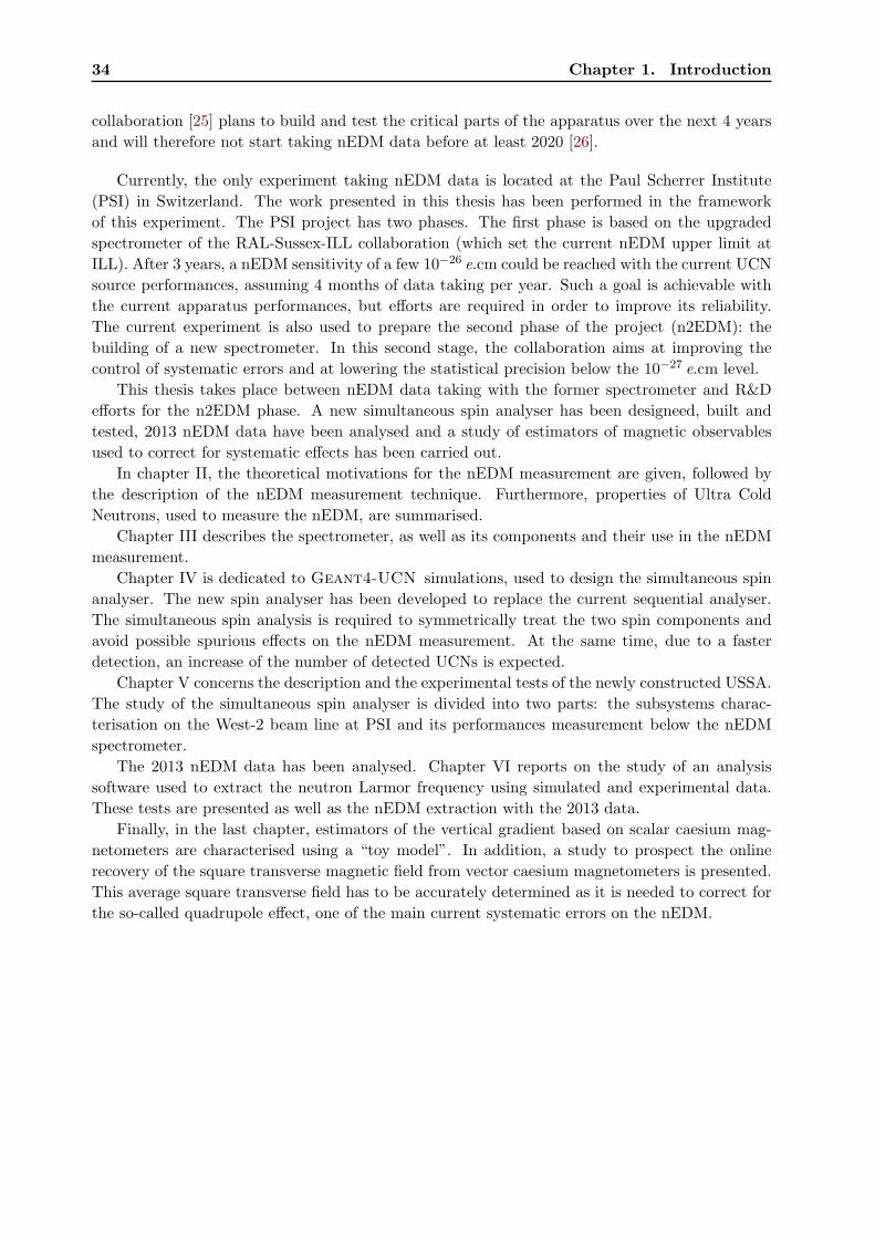
34 Chapter 1. Introduction

collaboration [25] plans to build and test the critical parts of the apparatus over the next 4 years

and will therefore not start taking nEDM data before at least 2020 [26].

Currently, the only experiment taking nEDM data is located at the Paul Scherrer Institute

(PSI) in Switzerland. The work presented in this thesis has been performed in the framework

of this experiment. The PSI project has two phases. The first phase is based on the upgraded

spectrometer of the RAL-Sussex-ILL collaboration (which set the current nEDM upper limit at

ILL). After 3 years, a nEDM sensitivity of a few 10−26 e.cm could be reached with the current UCN

source performances, assuming 4 months of data taking per year. Such a goal is achievable with

the current apparatus performances, but efforts are required in order to improve its reliability.

The current experiment is also used to prepare the second phase of the project (n2EDM): the

building of a new spectrometer. In this second stage, the collaboration aims at improving the

control of systematic errors and at lowering the statistical precision below the 10−27 e.cm level.

This thesis takes place between nEDM data taking with the former spectrometer and R&D

efforts for the n2EDM phase. A new simultaneous spin analyser has been designeed, built and

tested, 2013 nEDM data have been analysed and a study of estimators of magnetic observables

used to correct for systematic effects has been carried out.

In chapter II, the theoretical motivations for the nEDM measurement are given, followed by

the description of the nEDM measurement technique. Furthermore, properties of Ultra Cold

Neutrons, used to measure the nEDM, are summarised.

Chapter III describes the spectrometer, as well as its components and their use in the nEDM

measurement.

Chapter IV is dedicated to Geant4-UCN simulations, used to design the simultaneous spin

analyser. The new spin analyser has been developed to replace the current sequential analyser.

The simultaneous spin analysis is required to symmetrically treat the two spin components and

avoid possible spurious effects on the nEDM measurement. At the same time, due to a faster

detection, an increase of the number of detected UCNs is expected.

Chapter V concerns the description and the experimental tests of the newly constructed USSA.

The study of the simultaneous spin analyser is divided into two parts: the subsystems charac-

terisation on the West-2 beam line at PSI and its performances measurement below the nEDM

spectrometer.

The 2013 nEDM data has been analysed. Chapter VI reports on the study of an analysis

software used to extract the neutron Larmor frequency using simulated and experimental data.

These tests are presented as well as the nEDM extraction with the 2013 data.

Finally, in the last chapter, estimators of the vertical gradient based on scalar caesium mag-

netometers are characterised using a “toy model”. In addition, a study to prospect the online

recovery of the square transverse magnetic field from vector caesium magnetometers is presented.

This average square transverse field has to be accurately determined as it is needed to correct for

the so-called quadrupole effect, one of the main current systematic errors on the nEDM.

Chapter 2

The neutron Electric Dipole Moment

Contents

2.1 Motivations . . . . . . . . . . . . . . . . . . . . . . . . . . . . . . . . . . . . . 39

2.1.1 History of symmetry breaking and nEDM . . . . . . . . . . . . . . . . . . . . 39

2.1.2 The Universe Baryon Asymmetry problem . . . . . . . . . . . . . . . . . . . . 40

2.1.3 The nEDM in the SM . . . . . . . . . . . . . . . . . . . . . . . . . . . . . . . 40

2.1.4 The nEDM in extensions of the SM . . . . . . . . . . . . . . . . . . . . . . . 41

2.1.5 Other electric dipole moments . . . . . . . . . . . . . . . . . . . . . . . . . . 42

2.1.5.1 Paramagnetic atoms . . . . . . . . . . . . . . . . . . . . . . . . . . . 42

2.1.5.2 Diamagnetic atoms . . . . . . . . . . . . . . . . . . . . . . . . . . . 42

2.2 The nEDM measurement . . . . . . . . . . . . . . . . . . . . . . . . . . . . . 44

2.2.1 Principle . . . . . . . . . . . . . . . . . . . . . . . . . . . . . . . . . . . . . . 44

2.2.2 The experimental technique . . . . . . . . . . . . . . . . . . . . . . . . . . . . 44

2.2.2.1 Ramsey’s separate oscillating fields method . . . . . . . . . . . . . . 45

2.2.2.2 Expected statistical sensitivity . . . . . . . . . . . . . . . . . . . . . 46

2.2.3 nEDM measurement history . . . . . . . . . . . . . . . . . . . . . . . . . . . . 47

2.2.3.1 Cold neutron beam based experiments . . . . . . . . . . . . . . . . . 47

2.2.3.2 Ultra cold neutron source based experiments . . . . . . . . . . . . . 48

2.2.3.3 Current nEDM projects . . . . . . . . . . . . . . . . . . . . . . . . . 48

2.3 Ultra cold neutrons . . . . . . . . . . . . . . . . . . . . . . . . . . . . . . . . 50

2.3.1 From the neutron to the ultra cold neutron . . . . . . . . . . . . . . . . . . . 50

2.3.2 Ultra cold neutron interactions . . . . . . . . . . . . . . . . . . . . . . . . . . 51

2.3.2.1 Strong interaction . . . . . . . . . . . . . . . . . . . . . . . . . . . . 51

2.3.2.2 Magnetic interaction . . . . . . . . . . . . . . . . . . . . . . . . . . . 52

2.3.2.3 Gravity . . . . . . . . . . . . . . . . . . . . . . . . . . . . . . . . . . 53

2.3.2.4 Weak interaction . . . . . . . . . . . . . . . . . . . . . . . . . . . . . 54

2.3.3 Ultra cold neutron production . . . . . . . . . . . . . . . . . . . . . . . . . . 54

2.1. Motivations 39

2.1 Motivations

A permanent electric dipole moment (EDM)#–

d is usually defined when two opposite charges ±q

are separated by a distance r as#–

d = q #–r . Such an EDM is observed in systems for which the

barycentres of negative and positive charges do not coincide as for instance in the H2O molecule.

For a neutron, a permanent EDM can be quantumly defined as a vectorial intrinsic observable.

Because neutrons have a 1/2 spin, this EDM has to be aligned along their spin#–

S - the solely

intrinsic vectorial quantity for this particle - according to the Wigner-Eckart theorem. Such EDM

reads#–

dn = dn#–

S/S. In fact, the neutron EDM is the analogue of the magnetic moment # –µn, but

instead of coupling to a magnetic field#–

B, it couples to an electric field#–

E. The overall Hamiltonian

reads:

H = − #–

dn.#–

E − # –µn.#–

B (2.1)

However, these two dipole moments interactions behave differently with respect to the discrete

symmetries: charge conjugation symmetry C, parity symmetry P and time reversal symmetry T.

Tab. 2.1 summarises the transformation of usual physical observables under P and T. According

to transformations of(

# –

dn ,#–

E)

and(

# –µn ,#–

B)

under these P and T operators, depicted in Fig. 2.1,

one has:

− #–

dn.#–

EP−→ #–

dn.#–

E − # –µn.#–

BP−→ − # –µn.

#–

B

− #–

dn.#–

ET−→ #–

dn.#–

E − # –µn.#–

BP−→ − # –µn.

#–

B(2.2)

This also applies to other particles with a non-zero spin, which can have an EDM. Thus, a non-

zero EDM would be a signature of P and T violation and assuming the CPT theorem, a new CP

violation source.

Observable/Symmetry P T

Position #–r − #–r #–r

Time t t −t

Momentum #–p − #–p − #–p

Spin, Angular momentum#–

S#–

S − #–

S

Magnetic Dipole Moment #–µ #–µ − #–µ

Magnetic field#–

B#–

B − #–

B

Electric Dipole Moment#–

d#–

d − #–

d

Electric field#–

E − #–

E#–

E

Table 2.1: Transformation of usual physical

observables under P and T symmetries.

Figure 2.1:(

#–

dn ,#–

E)

and(

# –µn ,#–

B)

transfor-

mation under P and T symmetries.

2.1.1 History of symmetry breaking and nEDM

Purcell and Ramsey first had the idea to experimentally test discrete symmetries in 1950 [27] by

measuring the neutron Electric Dipole Moment (nEDM). This pioneering measurement gave the

first upper limit on the nEDM in 1957 [28]:

|dn| < 5× 10−20e.cm (2.3)

This measurement was carried out during a key period for particle physics, when the idea of parity

violation in weak processes was discussed by Lee and Yang in 1956 in order to solve the θ-τ puzzle

[29]. One year after, the first parity violation in a weak process was experimentally discovered by

40 Chapter 2. The neutron Electric Dipole Moment

Mrs Wu[30]. In this context, the neutron EDM limit reinforced the idea of T and CP conservation

[31, 32].

But in 1964, the interest for the neutron EDM measurement grew up with the first observed

CP violation in the K0 decay [33]. Indeed, particle physics theories including CP violation made

naturally appear the nEDM, which was one of the main constrain for these models. Today,

discovered sources of P and CP violations (K0, B0 [34, 35] and D0 [36] decays) are included in

the SM (through the δ phase in the CKM matrix) but the situation remains unchanged for the

role played by the nEDM to constrain theories beyond the SM [16, 37]. Those models propose

explanations for unexplained points by the SM. For instance, the SM does not answer a crucial

question: why the visible Universe is mostly made of matter?

2.1.2 The Universe Baryon Asymmetry problem

In the early Universe, antimatter and matter would have annihilated to produce photons, according

to the Big Bang theory [2]. Starting from the same amount of matter and antimatter, the Universe

should now be made of a small equal amount of matter and antimatter. The current Universe

composition is a proof that an asymmetric process occurred in the past since the antimatter is

nearly absent in the Universe [38].

In 1967, Sakharov1 proposed a scenario to explain this Baryon Asymmetry of the Universe

(BAU) [3], requiring three criteria to be fulfilled. First, a small violation of the baryon number B

is needed to allow a system to go from a B = 0 state to a B 6= 0 state. Then, C and CP violations

are required in order to slightly favour antimatter disappearance with respect to matter. Finally,

these processes have to occur during a non thermal equilibrium phase, otherwise, the reverse

processes would smooth out any matter or antimatter excess. In particle physics models, a first

order electroweak phase transition plays this role.

The matter-antimatter asymmetry in the universe can be estimated by the ratio:

η =nB − nB

nγ(2.4)

where nB/nB are respectively the number of baryons/anti-baryons and nγ is the number of pho-

tons.

From satellite observations of the Cosmic Microwave Background, this ratio has been estimated

to be η = (6.18± 0.15)× 10−10 [39]. This ratio is also an input for the Big Bang Nucleosynthesis

model which predicts the light nuclei abundances. In order to match measured abundances, the

η ratio is constrained to η = (5.80 ± 0.27) × 10−10 [40], which is consistent with the previous η

value.

There, the CP violation condition from the three Sakharov criteria becomes very important.

With all the CP violating processes found in the electroweak sector and incorporated in the SM,

the predicted matter-antimatter asymmetry ηSM ∼ 10−19 is 9 orders of magnitude smaller than

the experimental one. Thus, a strong motivation of SM extensions is to predict new CP violation

sources to get a baryonic asymmetry consistent with observations. In this context, the nEDM

searches are important since they may reveal new CP violation sources.

2.1.3 The nEDM in the SM

A neutron EDM could arise from two CP violation sources in the SM: one from the electroweak

sector and another one from the strong sector.

In the electroweak sector, a contribution to the nEDM can be calculated in a two quarks model

with a spectator quark [41]. This contribution of the electroweak sector to the nEDM amounts

1Peace Nobel price in 1975.

2.1. Motivations 41

to: |dn| ∼ 10−32−31 e.cm. Using the link between the CP violating phase in the CKM matrix

and the quarks EDM, another calculation has been performed, based on the fact that there is no

quark EDM contribution before 3 loops diagrams [42]. This contribution has been estimated to

|dn| ∼ 10−34 e.cm [43].

In the strong sector, the quantum chromodynamics Lagrangian can be split in two parts: one

concerning the quark-gluon interactions and the other one related to the interaction of gluons

with the quantum vacuum [44]. This latter, violating the CP symmetry, is related to the neutron

EDM via a theory-free angle θ. The parameter θ related to this angle θ is linked to the neutron

EDM through [15]:

|dn| ∼ θ × 10−16e.cm (2.5)

Today, the neutron EDM is the strongest constrain on the θ angle (through the θ parameter).

The best experimental limit on the nEDM [1] directly translates to a limit for θ < 10−10. This

constitutes the strong CP problem, as the natural range for θ is the unity. Peccei and Quinn have

tried to solve this problem by introducing an additional symmetry (U(1)PQ) [4]. In this model,

the θ value is 0 and a new particle, the axion, is involved during the spontaneous break of this

additional symmetry. This potential new particle has not been found yet. Thus, the strong CP

problem remains unsolved.

Up to now, the nEDM has already brought stringent constrains on the SM in the strong

sector. In the electroweak sector, SM predictions are currently out of reach. But extensions of

the Standard Model, including other CP violation sources, predict larger values for the nEDM,

in the 10−28 − 10−26 e.cm domain. As a result, it is possible to constrain these SM extensions by

measuring the nEDM (and other particles EDMs).

2.1.4 The nEDM in extensions of the SM

The Higgs search at LHC [5, 6] has confirmed what was hinted since about 20 years by EDM

measurements: no squark, predicted by supersymmetric (SUSY) models, have been found below

the TeV scale. This hint was triggered by the so-called SUSY CP problem: the upper limits

brought by the neutron, Tl and Hg EDMs have constrained the CP-odd SUSY phases θA and θµto ≃ 10−2, for SUSY particle masses MSUSY at the 500GeV level. These phases are (roughly)

constrained by EDMs d as follow [15]:

d×M2SUSY = aµ sin θµ + aA sin θA (2.6)

For a given EDM value and constant aµ and aA, the larger the SUSY mass scale, the larger the

θA and θµ free parameter space. By pushing mass limits of SUSY particles above the TeV scale,

LHC results have thus “resolved” this problem, as shown in Fig. 2.2. At the same time, several

SUSY models have been excluded.

The first order electroweak phase transition playing the role of the thermodynamic non-

equilibrium Sakharov criterion (see 2.1.2) is not allowed anymore in the SM [45]. On the contrary,

models of Electroweak Baryogenesis (EWBG) beyond the SM still allow this kind of transition

[46]. EDMs vary like 1/Λ2, where Λ is the new physics mass scale [15]. The power of EDMs

can be demonstrated by means of the following example: Fig. 2.3 shows the new physics particle

mass range excluded by EDMs in the framework of a minimal EWBG scenario [47]. Today, this

kind of scenarios has almost been excluded by the new limits set on the electron EDM and the

Hg EDM (see 2.1.5). However, an improvement of the nEDM limit below 10−27 e.cm in the next

experiments generation has the potential to rule out more elaborated models.

42 Chapter 2. The neutron Electric Dipole Moment

Figure 2.2: Illustration of the relaxation of the SUSY CP problem: constrains put by EDMs on

SUSY CP violating phases. Picture taken from [15].

2.1.5 Other electric dipole moments

As shown in Fig. 2.2, other electric dipole moments can constrain models beyond the SM. Projects

to measure directly the EDM of charged particles like protons, deuterons or muons on high pre-

cision rings are in development[48, 49]. There exist two types of atomic systems used for EDM

measurements: diamagnetic atoms and paramagnetic atoms and molecules [17].

2.1.5.1 Paramagnetic atoms

In the case of paramagnetic atoms, there is a single electron in the external electronic shell. The

contribution to the atomic EDM comes from the electron EDM by means of a relativistic effect

linked to the electron movement around the atom [50]. Without this effect, the Schiff screening

effect predicts that inside a neutral atom, electric charges arrange in such a way that the external

electric fields cancel [51]. As a result, there would be no induced atomic EDM by the single

electron EDM. Finally, the relation between the EDM of the paramagnetic atom dpar and the

electron EDM de is given by [15]:

dpar ≃ 10deZ3α2

J (J + 1/2) (J + 1)2(2.7)

where Z is the atomic number, α its polarisability and J its angular momentum. As the observable

EDM depends on the cube of the atomic number, heavy paramagnetic atoms are used to measure

de. As a result, the best current limit on the electron EDM coming from a paramagnetic atom

comes from the 205Tl EDM: |de| < 1.6× 10−27e.cm [52].

This limit has been confirmed using YbF molecules [53] and has recently been improved using

polar molecules of ThO down to |de| < 8.7× 10−29 e.cm [54]. This large increase of the sensitivity

is mainly due to the higher electric field obtained in polar molecules than in atoms.

2.1.5.2 Diamagnetic atoms

Diamagnetic atoms are probes for nuclear EDMs. Indeed, the Schiff theorem applies for these

atoms at first order but is violated at second order because of the finite size of nuclei. Unlike

paramagnetic atoms EDMs, diamagnetic atoms EDMs are smaller than the sum of their con-

stituents EDMs. As a result, the atom EDM comes from CP violating couplings between nucleons

2.1. Motivations 43

Figure 2.3: New physics mass exclusion areas in a minimal EWBG scenario due to EDMs limits

in 2007. The blue line corresponds to the threshold mass scale required to produce the baryon

asymmetry according to Sakharov criteria. Picture taken from [47].

and electrons and from couplings between nucleons. The present best limit on the 199Hg EDM is∣

∣d(199Hg)∣

∣ < 3.1× 10−29 e.cm [55], setting a limit on the proton EDM |dp| < 0.4× 10−23 e.cm.

44 Chapter 2. The neutron Electric Dipole Moment

2.2 The nEDM measurement

2.2.1 Principle

The principle of the nEDM measurement is visible through the interaction Hamiltonian of a

neutron in static magnetic and electric fields:

H = − # –

dn.#–

E − # –µn.#–

B (2.8)

In the presence of a magnetic field and an electric field, the energy levels split as shown in Fig. 2.4.

B = 0

E = 0

S↑B↑, E = 0

S↓B↑, E = 0

B↑, E↑

B↑, E↓

B↑, E↓

B↑, E↑

hν‖ = −2 (µnB + dnE) hν∦ = −2 (µnB − dnE)

−dnE

Figure 2.4: Scheme of the neutron energy levels splitting of a neutron in magnetic and electric

fields. Subscripts ‖ and ∦ correspond respectively to parallel and anti-parallel#–

B and#–

E fields

configurations. It is assumed that dn and µn have the same sign.

The nEDM is then measured via the difference of Larmor frequencies ν‖ and ν∦ in parallel and

anti-parallel static magnetic and electric fields through:

dn =−h(ν‖ − ν∦)− 2µn(B‖ −B∦)

2(E‖ + E∦)(2.9)

Because the magnetic interaction is dominant, the experimental strategy is always to apply a low

magnetic field and a large electric field. In the case where the B field is unchanged in parallel and

anti-parallel configuration and the electric field only changes its sign, the nEDM is given by:

dn =−h(ν‖ − ν∦)

4E(2.10)

The neutrons precession frequency is measured using the Ramsey’s separated oscillating fields

method. This method is explained in the following paragraph.

2.2.2 The experimental technique

The experimental technique used to determine the neutron Larmor frequency is the same for all

storage experiments. Polarized ultra cold neutrons are stored in a precession chamber and the

number of remaining spin up and spin down neutrons are counted after the Ramsey’s separate

oscillating fields procedure. This procedure is part of a cycle. It is repeated several times for a

given magnetic and electric fields configuration. The Ramsey’s method was used for nEDM beam

measurements, but the oscillating fields were spatially separated instead of timely separated. This

method is described thereafter and sketched out in Fig. 2.5.

2.2. The nEDM measurement 45

2.2.2.1 Ramsey’s separate oscillating fields method

B E

B E

RF pulse RF pulse

PolarizedUCNs

Free precession

UCNcounting

Figure 2.5: Principle of the Ramsey separated oscillating field method.

Polarized ultracold neutrons are stored in a precession chamber where parallel or antiparallel

magnetic and electric fields are applied. The UCN spin is initially aligned along the main magnetic

field B0. During a short period τRF, a radiofrequency (RF) pulse with a frequency in principle

equal to the neutron Larmor frequency fn = γn2πB0 is applied. As a result, the neutron spin is

flipped into the plane orthogonal to the static magnetic field and the applied RF pulse is called π/2

pulse. Neutrons are then free to precess during a time T ≫ τRF. At the end of the precession time

T , a second π/2 pulse is applied with the same frequency as the first one. A phase is accumulated

during the free precession if dn 6= 0. This leads to a frequency shift. The actual Larmor frequency

is determined by slighly detuning the RF pulse frequency and by counting the spin up and the

spin down neutrons, in order to scan the so-called Ramsey pattern, shown in Fig. 2.6.

[Hz]RFf

30.12 30.14 30.16 30.18 30.2

Norm

ali

zed N

eutr

on C

ounts

6000

8000

10000

12000

14000

16000

18000↑

N

↓N

Figure 2.6: Ramsey pattern obtained in August 2012 after 50 s of precession in the oILL spec-

trometer at PSI. The most populated spin state at the beginning of each cycle is N↓.

In practice, only the Ramsey central fringe is scanned. Four working points, placed where

the slope is the steepest, are used in order to increase the sensitivity of the Larmor frequency

46 Chapter 2. The neutron Electric Dipole Moment

measurement. For an initial spin up population, this central fringe is approximated by:

N↑/↓ = N↑/↓0

(

1∓ α↑/↓ cos

[

(fn − fRF )

∆νπ

])

(2.11)

where ∆ν = 12(T+4τ/π) is the half width of the central fringe, N

↑/↓0 the number of detected

neutrons for each spin state at half the resonnance with sign −/+ corresponding respectively

to spin up/down UCNs. α↑/↓ is the visibility of the fringe defined as:

α↑/↓ =N

↑/↓max −N

↑/↓min

N↑/↓max +N

↑/↓min

(2.12)

Using a best fit of N↑ and N↓ with (2.11), the neutron Larmor frequency is determined for both

parallel and antiparallel magnetic and electric fields.

2.2.2.2 Expected statistical sensitivity

From (2.11), it is possible to get the expression of the neutron Larmor frequency as a function of

the number of detected neutrons:

f↑/↓n = fRF +

∆ν

πarccos

(

N↑/↓ −N↑/↓0

∓α↑/↓N↑/↓0

)

(2.13)

and the statistical error on the neutron precession frequency is determined through:

σ↑/↓fn

2=

(

∂fn

∂N↑/↓σN↑/↓

)2

+

(

∂fn

∂N↑/↓0

σN

↑/↓0

)2

+

(

∂fn

∂α↑/↓σα↑/↓

)2

σ↑/↓fn

2=

(

∆ν

πα↑/↓N↑/↓0

)2

× 1

1−(

N↑/↓0 −N↑/↓

N↑/↓0 α↑/↓

)2

×

N↑/↓ +

(

σN

↑/↓0

N↑/↓

N↑/↓0

)2

+(

(N↑/↓ −N↑/↓0 )

σα↑/↓

α↑/↓

)2

(2.14)

The two last terms contribution (with σN

↑/↓0

and σα↑/↓) corresponds to about 1% of the total error.

In the present case, the four working points are around half of the resonnance, i.e. N↑/↓ ≃ N↑/↓0 .

Thus, the statistical uncertainty on the neutron Larmor frequency is approximated by:

σ↑/↓fn

≃ ∆ν

πα↑/↓√N↑/↓

(2.15)

Using (2.10), the statistical error on the nEDM becomes:

σdn =

√

σ‖fn

2+ σ

∦fn

2 h

4E(2.16)

σdn ≃ ~

2αTE√Ntot

(2.17)

The last formula gives the experimental key observables of the nEDM statistical sensitivity. The

higher the applied electric field, the larger the nEDM sensivity. At the same time, increasing the

precession time would allow neutrons to accumulate more phase during the free precession. The

visibility of the central fringe exponentially decreases with the precession time. It depends on

2.2. The nEDM measurement 47

precession chamber properties and on magnetic field conditions (UCN spin guiding fields and field

homogeneity in the precession chamber). It also depends on the neutron spin analysis efficiency.

The number of ultracold neutrons detected at the end of the precession also depends on precession

chamber properties and roughly decreases exponentially with the precession time. Therefore, the

setting of the precession time is closely linked to the central fringe visibility and the number of

detected UCNs. This storage time was tuned to about 200 s in [56] for the nEDM experiment at

PSI.

All the parameters have to be as high as possible in order to lower the statistical error σdn .

But there is some interplay between T , E and Ntot. During the nEDM history, the game has

always been to increase these parameters, but also to lower the systematic errors.

2.2.3 nEDM measurement history

The evolution of the nEDM upper limit is shown in Fig. 2.7. Two main types of measurement are

visible: beam and storage measurements.

10-34

10-33

10-32

1950 1960 1970 1980 1990 2000 2010 2020

Year

10-28

10-26

10-24

10-22

10-20

10-18

nE

DM

upper

lim

it [

e.cm

]

10-28

10-26

10-24

10-22

10-20

10-18

nE

DM

upper

lim

it [

e.cm

]

Beam exp.Diffusion exp.Storage PNPI

Storage ILL

New Physics

Standard Model

Figure 2.7: nEDM upper limit history.

2.2.3.1 Cold neutron beam based experiments

The first dedicated nEDM measurement was carried out by Smith, Purcell and Ramsey in 1957,

setting the upper limit |dn| < 5 × 10−20 e.cm [28]. The experiment used a 2000m/s polarised

neutron beam going through a homogeneous magnetic field in which the neutron spin precesses.

During the experiment, an electric field was applied and the authors did not measure any correla-

tion with the neutron precession frequency. These beam line experiments have continued during

about 20 years, until the first ultra cold neutron sources were built in the 80’s. nEDM mea-

surements with these slower neutrons (vn <5m/s) are better for two main reasons. First, slow

neutrons spend more time in the electric field area. Second, the so-called geometric-phase effect

is reduced [8]. The consequence of this relativistic effect is that moving neutrons see a motional

magnetic field#–

Bv =#–

E#–×vnc2

. As a result, the neutron precession frequency is shifted proportionally

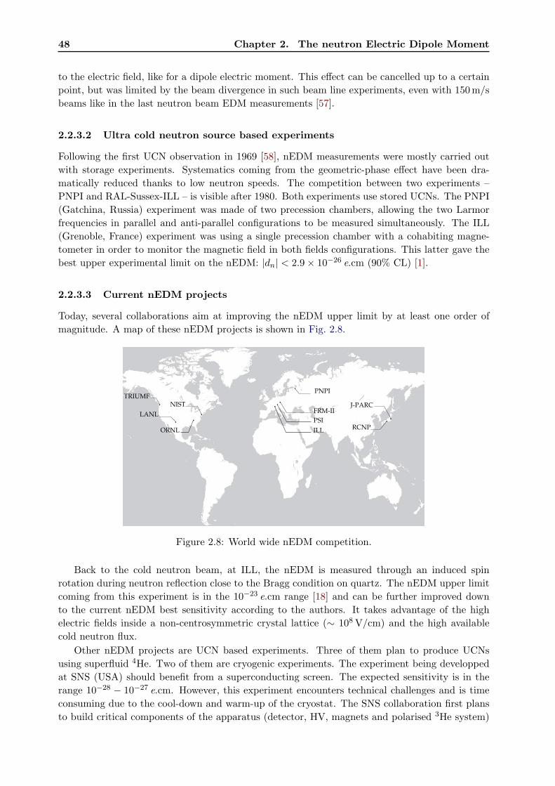
48 Chapter 2. The neutron Electric Dipole Moment

to the electric field, like for a dipole electric moment. This effect can be cancelled up to a certain

point, but was limited by the beam divergence in such beam line experiments, even with 150m/s

beams like in the last neutron beam EDM measurements [57].

2.2.3.2 Ultra cold neutron source based experiments

Following the first UCN observation in 1969 [58], nEDM measurements were mostly carried out

with storage experiments. Systematics coming from the geometric-phase effect have been dra-

matically reduced thanks to low neutron speeds. The competition between two experiments –

PNPI and RAL-Sussex-ILL – is visible after 1980. Both experiments use stored UCNs. The PNPI

(Gatchina, Russia) experiment was made of two precession chambers, allowing the two Larmor

frequencies in parallel and anti-parallel configurations to be measured simultaneously. The ILL

(Grenoble, France) experiment was using a single precession chamber with a cohabiting magne-

tometer in order to monitor the magnetic field in both fields configurations. This latter gave the

best upper experimental limit on the nEDM: |dn| < 2.9× 10−26 e.cm (90% CL) [1].

2.2.3.3 Current nEDM projects

Today, several collaborations aim at improving the nEDM upper limit by at least one order of

magnitude. A map of these nEDM projects is shown in Fig. 2.8.

PNPI

FRM-II

PSI

ILL

J-PARC

RCNP

TRIUMF

LANL

ORNL

NIST

Figure 2.8: World wide nEDM competition.

Back to the cold neutron beam, at ILL, the nEDM is measured through an induced spin

rotation during neutron reflection close to the Bragg condition on quartz. The nEDM upper limit

coming from this experiment is in the 10−23 e.cm range [18] and can be further improved down

to the current nEDM best sensitivity according to the authors. It takes advantage of the high

electric fields inside a non-centrosymmetric crystal lattice (∼ 108V/cm) and the high available

cold neutron flux.

Other nEDM projects are UCN based experiments. Three of them plan to produce UCNs

using superfluid 4He. Two of them are cryogenic experiments. The experiment being developped

at SNS (USA) should benefit from a superconducting screen. The expected sensitivity is in the

range 10−28 − 10−27 e.cm. However, this experiment encounters technical challenges and is time

consuming due to the cool-down and warm-up of the cryostat. The SNS collaboration first plans

to build critical components of the apparatus (detector, HV, magnets and polarised 3He system)

2.2. The nEDM measurement 49

Experiment Source Cell Measurement technique

ILL - CryoEDM Superfluid 4He 4He Cryo HV, Superconducting tech.

- UCN - νL Ramsey tech., SQUIDS

SNS - EDM Superfluid 4He 4He Cryo HV, Superconducting tech., SQUIDS

- UCN - νL:3He capture, 3He co-magnetometer

RCNP - TRIUMF Superfluid 4He Vacuum Small volume, 129Xe co-magnetomer

- UCN - @RNCP and then @TRIUMF

ILL - PNPI ILL turbine Vacuum νL: Ramsey tech.

- UCN - PNPI:Solid D2 E = 0 for magnetometer

PSI EDM Solid D2 Vacuum νL: Ramsey tech., Hg co-magnetometer

- UCN - 132Cs, 3He external magnetometers

MUNICH - FRMII Solid D2 Vacuum νL: Ramsey tech., Hg co-magnetometer

- UCN - Cs external magnetometer

J-PARC - UCN Solid D2 Vacuum Under development

LANL - UCN Solid D2 Vacuum Under development

ILL-PNPI Cold n. beam Solid Crystal diffraction

Non-centrosymmetric crystal

J-PARC Cold n. beam Solid Crystal diffraction

Non-centrosymmetric crystal

NIST Crystal Solid R & D

Table 2.2: Worldwide nEDM projects in competition. From [59]

and to test it at the NCSU2 reactor over the next 4 years. Once this will be done, they could

get approval to finish the construction of the cryogenic system, the neutron beam guide and the

room temperature magnetic shield [26]. CryoEDM project at ILL [60], one of the most important

nEDM projects, was recently stopped due to funding cutoff.

Room temperature experiments aim at measuring the nEDM at the 10−28 − 10−27 e.cm level.

Among those, a project is being built at the Research Center of Nuclear Physics (RCNP) in

Japan [23] and will be later moved to TRIUMF in Canada. This project, based on previous room-

temperature measurements, plans to use a Xe buffer gas inside the precession volume in order to

suppress the so-called systematic geometric phase effect.

A recent measurement performed at ILL with the PNPI spectrometer (a stack of two precession

chambers placed in a common magnetic field) by Serebrov et al. reports an nEDM upper limit of

|dn| < 5.5× 10−26 e.cm [20]. A later stage is planned at a new UCN source at PNPI.

At FRM-II, the Munich collaboration plans to use a four-layer stack of precession chambers

(two with UCNs and a Hg co-magnetometer, two with only Hg). It also plans to use external

Caesium magnetometers in order to have a better control on systematics. The progress with the

apparatus is going fast (the magnetic shield is already installed). However, the UCN source has

not started yet.

The other main room temperature project is the nEDM experiment at PSI, which aims at mea-

suring the nEDM below the 10−27 e.cm level in two phases. The first phase uses the spectrometer

which belonged to the RAL-Sussex-ILL collaboration. The spectrometer has been moved in 2009

to the new PSI UCN source and renamed oILL for old ILL spectrometer. The second phase is

based on the development of a new spectrometer (n2EDM) involving two UCN storage chambers.

All these last experiments are based on the ultra cold neutrons use. Their properties are

summarized in the next part.

2North Carolina State University

50 Chapter 2. The neutron Electric Dipole Moment

2.3 Ultra cold neutrons

The neutron electric dipole moment search is closely linked to the development of ultra cold

neutron sources. Neutrons are called ultra cold when a particular energy regime is reached, below

a few hundred neV. A short summary of different neutron regimes is given in this section, followed

by a description of ultra cold neutron properties and different ways to produce them.

2.3.1 From the neutron to the ultra cold neutron

The neutron was discovered in 1932 by Chadwick [61]. Fast neutrons are mainly produced during

fission or spallation reactions. Today, they are widely used to study materials, thanks to their

property to deeply penetrate into matter because of their neutrality. They can be thermalized

using collisions with light nuclei. Because neutrons show particular properties for different energy

ranges, they are usually classified in different regimes (see Tab. 2.3), according to their kinetic

energy, temperature or wavelength.

Regime Energy Wavelength [nm] Temperature [K]

Fast > 500 keV < 10−3 > 6× 106

Epithermal 25meV < E < 500 keV 10−3 < λ < 0.18 300 < T < 6× 106

Thermal 25meV 0.18 300

Cold 50µeV < E < 25meV 0.18 < λ < 4 0.6 < T < 300

Very cold 300 neV < E < 50µeV 4 < λ < 52 0.0035 < T < 0.6

Ultra cold < 300 neV >52 <0.0035

Table 2.3: Different neutron energy regimes and characteristic energy, wavelength, temperature

ranges. The blue shaded rows correspond to optical neutrons.

The neutrons De Broglie wavelength λn is defined as follow:

λn =h√

2mnE(2.18)

where mn is the neutron mass and E the neutron kinetic energy. When the neutron wavelength

becomes larger than the distance between atoms of a material - neutrons are cooler - neutrons

interact with a set of nuclei instead of a single nucleus. These neutrons are called optical neutrons

(E < 25meV, λ > 0.2 nm) and can be reflected by matter as observed by Fermi in 1947 [62]. Such

reflexion happens if the incidence angle θ fulfils the following condition:

sin θ ≤√

VF

E(2.19)

where VF is the so-called Fermi potential or optical potential. It is one of the most important

characteristic for UCNs and is defined as:

VF =2π~2

mn

∑

i

Nibi (2.20)

where Ni is the number of atoms per volume unit and bi is the coherent scattering length of the

nuclei constituting the material. A typical order of magnitude for the Fermi potential is a few

hundred neV. Eq (2.19) shows an interesting property of neutrons: neutrons with lower energies

than the Fermi potential are reflected whatever the incidence angle θ. In that case, one speaks

about ultra cold neutrons (UCN). It is therefore possible to store them in material bottles. The

existence of such very slow and storable neutrons was predicted by Zel’dovich in 1959 [63] and

first experienced by Shapiro’s group in 1969 [58].

2.3. Ultra cold neutrons 51

2.3.2 Ultra cold neutron interactions

The UCNs particularity is that their kinetic energy is of the same order of magnitude as the

energy associated to each fundamental interaction (except for the weak interaction).

2.3.2.1 Strong interaction

The strong interaction governs the UCNs interaction with matter, leading to their reflection or

their absorption. A thorough study of UCNs interactions is given in [64]. Classically, UCNs with a

lower energy than the Fermi potential are always reflected. Quantumly, the collision of a neutron

with kinetic energy E with a material surface is described by the stationary Schrodinger equation:

−~2

2mn∆Ψ+ VΨ = EΨ (2.21)

V = 0 x < 0

V = VF + iW x > 0(2.22)

where VF is the Fermi potential calculated in (2.20). This term is the volumic average of an

effective potential taking into account a collection of nuclei at positions #–ri:

U( #–r ) =2π~2

mn

∑

i

biδ(#–r − #–ri) (2.23)

This potential was introduced by Fermi [65] in order to describe a slow neutron diffusion (< 1 eV)

on a set of nuclear potentials (∼ 40MeV), without using the perturbation theory (because the

interaction potential is much larger than UCN energies).

The imaginary part W reflects the possibility for UCNs to be absorbed or up-scattered during

a reflection if the wave function penetrates the potential wall (in both cases, the neutron is lost).

For UCNs, both the absorption and the up-scattering cross-sections are inversely proportional to

the neutron velocity vn [64]. W is calculated using absorption and up-scattering cross-sections σaand σus:

W =~vn2

∑

i

Ni

(

σia + σi

us

)

(2.24)

Thus, in the low energy regime i.e. for UCNs, W is independent of the neutron velocity.

The neutron wave function behaviour is described by (see Fig. 2.9):

Ψ =

eikxx +Re−ikxx x < 0

Teiktx x > 0(2.25)

with kx =√

2mn~2

.E⊥ and kt =√

2mn~2

. (E⊥ − VF ). Where E⊥ is the orthogonal component of the

energy, R and T are respectively the amplitudes of the reflected and transmitted waves. Thanks

to the continuity conditions at x = 0, the amplitude of the reflected wave is given by:

R =

√E⊥ −

√E⊥ − V√

E⊥ +√E⊥ − V

(2.26)

In the majority of cases W ≪ VF , which leads to a reflection probability:

R2 =

(

1−√

1−VF /E⊥

1+√

1−VF /E⊥

)2

E⊥ > VF

|R|2 = 1− 2WVF

√

E⊥

VF−E⊥E⊥ < VF

(2.27)

52 Chapter 2. The neutron Electric Dipole Moment

Reflected wave:

Incident wave:

Transmitted wave:

x=0

Figure 2.9: Scheme of the neutron interaction with a material surface.

Even with E⊥ < VF , neutrons have a probability to be lost proportional to W , due to the

evanescent transmitted wave function. The loss probability per bounce µ is defined as:

µ(E⊥) = 1− |R|2 = η

√

E⊥VF − E⊥

(2.28)

with η = 2WVF

the loss factor. This loss factor is a characteristic of the material used and is at the

10−5 − 10−4 range.

Thus, when UCNs reach a material wall, they can be either reflected or transmitted through

the wall according to Eq (2.27). But the reflection process can occur in two different ways. The

neutron specular reflection is well suited in the case of a perfectly flat wall surface. But in the case

where the surface exhibits some roughness, reflections can be either specular or diffuse. When

a diffuse reflection occurs, the UCN reflection direction is given by Lambert’s cosine law: the

probability for a UCN to be reflected with an angle θ from the surface normal in the solid angle

dΩ is given by cos θdΩ.

Thanks to the strong interaction of UCNs with a material wall, the UCN storage is possible.

Moreover, thanks to the diffuse reflection process, a mechanical equilibrium can be reached, leading

to the isotropy of the UCN speed distribution, as for a gas.

2.3.2.2 Magnetic interaction

UCN polarisation UCNs interact with magnetic fields by means of their magnetic moment

µn = −9.6623647(23)× 10−27 JT−1 [66]. The resulting potential energy is:

Vmag = − # –µn.#–

B (2.29)

For convenience, the magnetic moment can be expressed as µn ≃ 60.3 neV/T. It means that

UCNs crossing a 5T magnetic field region experience a ±300 neV potential if they have their spin

parallel or anti-parallel to the field direction (the magnetic moment is anti-parallel to the spin).

As a result, it is possible to use a sole magnetic field to polarise UCNs, as shown in Fig. 2.10.

Magnetic fields can also be used as magnetic shutters or fully magnetic traps. This method is

used in order to avoid losses due to wall interactions [67, 68].

Polarisation handling Considering the spin as a classical angular momentum ( even if a quan-

tum approach is more appropriate for a spin as in [69]), the magnetic field exerts a torque on the

UCN spin#–

S and gives the following time dependence:

d#–

S

dt= γn

#–

S × #–

B (2.30)

The Bloch equations (2.30) [70] describe the spin evolution in the presence of a magnetic field.

The spin precesses around the magnetic field at the Larmor angular frequency:

ωn = γnB = ωL (2.31)

2.3. Ultra cold neutrons 53

Figure 2.10: Scheme of the UCN polarisation process using a magnetic field barrier.

Like for Nuclear Magnetic Resonance (NMR) applications, longitudinal and transverse relaxation

times T1 and T2 are added to (2.30) in order to take into account depolarisation. Assuming the

main field direction along z, Eq (2.30) becomes for an ensemble of spins:

dSx,y

dt= γn

(

#–

S × #–

B)

x,y− Sx,y

T2

dSz

dt= γn

(

#–

S × #–

B)

z− Sz − S0

T1

(2.32)

where S0 is the asymptotic value of Sz. In the PSI experiment, the longitudinal relaxation time

T1, related to wall depolarisation’s is above the 1000 s level while the transverse relaxation time

T2, related to the homogeneity of the magnetic field is about 600 s with homogeneous field and

weak gradient.

2.3.2.3 Gravity

As for all massive particles, UCNs are sensitive to gravity. Their gravitational potential energy of

the same order as their kinetic energy and is given by:

Ep = mngz (2.33)

where mng ≃ 102.6 neV/m. As a result, a 100 neV UCN can not rise above 1m. This property

can be used to vertically store them or to increase the UCN detector efficiency by letting them

fall down to the detector (see 3.5.1). The effect of the gravitation on their trajectories is clearly

visible as shown in Fig. 2.11.

Figure 2.11: Parabolic UCN trajectories simulated using Geant4-UCN, as an example of the

gravity effect on ultra cold neutrons.

Because ultra cold neutrons have a very low energy, they can be used to characterize gravita-

tional quantum states [71].

54 Chapter 2. The neutron Electric Dipole Moment

2.3.2.4 Weak interaction

The weak interaction is responsible of the neutron β decay as shown by the artistic Feynman

diagram depicted in Fig. 2.12.

Figure 2.12: Feynman diagram of the neutron β decay.

The neutron lifetime τn = 880.0±0.9 s [72] is large enough to allow a long UCN storage. Thus,

stored UCNs are used to determine τn which plays a role in the Big-Bang Nucleosynthesis and in

the determination of the Vud term, needed for the test of the CKM matrix unitarity [73]. UCNs

are also used to perform angular correlation measurements in the neutron decay [74].

2.3.3 Ultra cold neutron production

Fast neutrons are produced either in reactors, through the fission process or with spallation process

on heavy nuclei targets. They are then cooled down to the cold neutron regime in light nuclei

volumes (heavy water, polyethylene moderators, deuterium...). Finally, cold neutrons are down

scattered to the ultra cold regime by phonon excitation in superfluid He or in solid D2 crystal. In

order to suppress the reverse process, the moderator is cooled down to very low temperatures.

Another way to cool down neutrons to the ultra cold regime is to use the gravitational deceler-

ation. This method is used at the ILL combined to the so called Steyerl turbine which lowers the

neutron energy spectrum by about a factor 100 down to the 100 neV range using multiple neutron

reflections on rotating nickel coated curved blades [75].

The UCN sources development is closely linked to the nEDM measurement projects. Indeed,

the nEDM experiments need high density UCN sources in order to lower the statistical error.

A summary of UCN sources projects with expected performances and characteristics is given in

Tab. 2.4. The PSI UCN source working principle is described in the following chapter, in the

context of the nEDM experiment at PSI.

2.3. Ultra cold neutrons 55

LocationNeutron

ModeratorExpected UCN

Statusproduction density [cm−3]

ILL, PF2 (France) Reactor Liquid D2+ Turbine 50 Working

PSI (Switzerland) Spallation Solid D2 >500 Working

Triga (Germany) Reactor Solid D2 10 Working

FRM-II (Germany) Reactor Solid D2 10000 >2015

LANL (USA) Spallation Solid D2 120 Working

RCNP (Japan) Spallation Superfluid He 15 Working

Triumf (Canada) Spallation Superfluid He 5800 >2015

PNPI (Russia) Reactor Superfluid He 10000 >2015

ILL, H172 (France) Reactor Superfluid He >1000 >2014

SNS (USA) Spallation Superfluid He 150 Working

Table 2.4: Summary of UCN source projects with initial expected UCN densities.

Chapter 3

The nEDM experiment @ PSI

Contents

3.1 The PSI ultra cold neutron source . . . . . . . . . . . . . . . . . . . . . . . 60

3.2 Experimental apparatus . . . . . . . . . . . . . . . . . . . . . . . . . . . . . 60

3.3 UCN transport and polarisation . . . . . . . . . . . . . . . . . . . . . . . . 61

3.3.1 NiMo coated guides . . . . . . . . . . . . . . . . . . . . . . . . . . . . . . . . 61

3.3.2 Super Conducting Magnet . . . . . . . . . . . . . . . . . . . . . . . . . . . . . 61

3.3.3 Guiding coils system . . . . . . . . . . . . . . . . . . . . . . . . . . . . . . . . 62

3.3.4 Switch box . . . . . . . . . . . . . . . . . . . . . . . . . . . . . . . . . . . . . 63

3.3.5 UCN storage chamber . . . . . . . . . . . . . . . . . . . . . . . . . . . . . . . 63

3.4 Magnetic field control . . . . . . . . . . . . . . . . . . . . . . . . . . . . . . . 64

3.4.1 Magnetic field production . . . . . . . . . . . . . . . . . . . . . . . . . . . . . 64

3.4.1.1 B0 coil . . . . . . . . . . . . . . . . . . . . . . . . . . . . . . . . . . 64

3.4.1.2 Hg and neutron radio-frequency coils . . . . . . . . . . . . . . . . . 64

3.4.1.3 Correcting coils . . . . . . . . . . . . . . . . . . . . . . . . . . . . . 64

3.4.2 Magnetic field stabilisation . . . . . . . . . . . . . . . . . . . . . . . . . . . . 65

3.4.2.1 Static magnetic shield . . . . . . . . . . . . . . . . . . . . . . . . . 65

3.4.2.2 Surrounding Field Compensation (SFC) . . . . . . . . . . . . . . . . 66

3.4.3 Magnetic field monitoring . . . . . . . . . . . . . . . . . . . . . . . . . . . . . 66

3.4.3.1 Mercury cohabiting magnetometer . . . . . . . . . . . . . . . . . . . 66

3.4.3.2 Caesium magnetometers array . . . . . . . . . . . . . . . . . . . . . 67

3.5 UCN spin analysis and detection . . . . . . . . . . . . . . . . . . . . . . . . 68

3.5.1 Neutron detector . . . . . . . . . . . . . . . . . . . . . . . . . . . . . . . . . . 68

3.5.2 Spin analysing system . . . . . . . . . . . . . . . . . . . . . . . . . . . . . . . 69

3.5.2.1 The spin analyser . . . . . . . . . . . . . . . . . . . . . . . . . . . . 70

3.5.2.2 The adiabatic spin-flipper . . . . . . . . . . . . . . . . . . . . . . . . 70

3.5.2.3 The sequential spin analysis . . . . . . . . . . . . . . . . . . . . . . 71

59

The nEDM experiment at PSI is supported by a collaboration of 12 European laboratories.

The project is divided in three stages. First, the collaboration restarted operating the oILL

spectrometer at ILL between 2005 and 2009. This spectrometer, operating at room temperature,

holds the best nEDM limit [1]. During this time period, the spectrometer was restarted and

refurbished. Then, it was moved to the new UCN source developed at the Paul Scherrer Institute

in 2009 in order to take nEDM data and reach the 10−27 e.cm level. This goal has been recently

reviewed to 10−26e.cm, if source performances stay lower than former expectations. Finally, in

the last phase of the experiment, a new spectrometer will be constructed. It has been designed to

increase UCN statistics and to allow a better control on systematic effects.

Today, the nEDM experiment is installed in the West area at the PSI. Because the PSI houses

a wide range of facilities in various topics, the nEDM experiment has also some rather close

and large magnetic devices like the SULTAN 1 or EDIPO 2 magnets (see Fig. 3.1). They create

magnetic fields up to 12T at their centre. Once they are operating in a steady state, these magnets

are not problematic anymore, thanks to the Surrounding Field Compensation (SFC) system (see

3.4.2.2). However, during the ramping up and down of the magnets, it is not possible to take

nEDM data due to the magnetic field variations. This problem can not be circumvented because

the nEDM apparatus has to be located close to the PSI UCN source, in order to get as many

ultra cold neutrons as possible. This source, commissioned in 2011, is shortly described in the

following section.

ExperimentalHall

UCN source

nEDM

Cyclotron ring

SINQ Hall

SULTAN magnet

220 m

Muon physics

Figure 3.1: Facility site plan of the PSI West area where the nEDM experiment is located.

1SUpraLeiter Test ANlage: superconductor test facility.2European Dipole project: used for instance in ITER conductors tests.

60 Chapter 3. The nEDM experiment @ PSI

3.1 The PSI ultra cold neutron source

The PSI UCN source uses the fast proton beam delivered by the PSI cyclotron. In usual conditions,

the source is operated with the full 590MeV proton beam at 2.2mA with a duty cycle around

1%. The proton beam is delivered during 3 or 4 s every 360 s or 480 s, according to users needs.

A scheme of the PSI UCN source is shown in Fig. 3.2 and a detailed description of the

source can be found in [76]. During the proton pulse, fast neutrons are produced by spallation

on a lead target. These neutrons are then thermalized in a volume of heavy water. Finally,

cold and ultra cold neutrons are produced in a 30 ℓ solid deuterium (sD2) crystal at 5K. Such a

technique to produce ultra cold neutrons was initially proposed by Golub and Pendlebury [77] and

is called superthermal UCN production. It uses the phonons excitation in the crystal lattice which

leaves incoming neutrons with almost no energy. The reverse process is suppressed by the low

temperature of the converter. UCNs are then filled into a Diamond-Like Carbon (DLC) coated

storage vessel before being distributed towards different UCN beam ports. The West-1 beam

port, used to check the UCN source performances, provides about 25 × 106 detected UCNs for

4 s proton kicks. A measurement performed at this beam port using a 25 ℓ NiMo coated storage

volume has shown a density above 30 UCNs/cm3 after 3 s storage. The West-2 port is dedicated

to UCN users for tests or experiments. The last port (South one), is connected to the nEDM

experiment whose apparatus is described in the following section.

Lead target

Liquid

UCN storage vessel

Bend

Coolant and supplylines

South port

West-2 port

West-1 port

Protons

1 m

Figure 3.2: Sketch of the PSI ultra cold neutron source with its three available beam ports. The

nEDM experiment is connected to the South beam port.

3.2 Experimental apparatus

For the current data taking, the former oILL spectrometer has been upgraded and moved to the

Paul Scherrer Institute in 2009. The nEDM apparatus is shown in Fig. 3.3. The nEDM apparatus

is enclosed in a wooden non-magnetic thermohouse with an air conditioning system in order to

3.3. UCN transport and polarisation 61

stabilise the temperature at the 0.5-1K level. The components of the nEDM apparatus and their

role are described. For an exhaustive description of the experimental setup, see [56].

Figure 3.3: Sketch of the nEDM apparatus. The big surrounding field compensation coils (SFC)

are not shown. On the bottom right corner of this figure, the nEDM reference frame axes used

throughout this work is defined. It is centred on the Hg readout level at the centre of the precession

chamber.

UCNs coming from the source first cross a super conducting magnet (SCM) which acts as a

polariser. Then, they are guided towards the storage chamber via a switch box, used to provide

neutrons in different parts of the experiment. After a precessing period, UCNs fall down to the

spin analyser and are finally detected in the UCN detector.

3.3 UCN transport and polarisation

Downstream to the SCM, neutrons are transported towards the experiment within glass guides.

Additional magnetic fields are used in order to keep the UCN polarisation along their way towards

the precession chamber.

3.3.1 NiMo coated guides

In the experiment, glass guides of 73mm inner diameter with a NiMo coating are used to transport

UCNs. The same glass guides (with a larger diameter) are also used to bring neutrons from the

UCN source to the SCM entrance. The NiMo coating is usually used in UCN transport because

its Fermi potential is rather large (220 neV) and its weak depolarisation probability per bounce

(∼ 10−5) is appropriate to keep the UCN polarisation. These properties allow for a good UCN

transmission.

3.3.2 Super Conducting Magnet

A super conducting magnet is located between the UCN tank and the nEDM apparatus. The SCM

is used to polarise UCNs: when they are guided through the 5T SCM, neutrons with less than

62 Chapter 3. The nEDM experiment @ PSI

300 neV can be polarised. Indeed, neutrons with the wrong spin state are not able to cross the

magnetic potential energy created by the SCM and are reflected back to the UCN tank. Because

the UCN guides Fermi potential is around 220 neV, it is assumed that there are no UCNs with

energies larger than 300 neV. Therefore, it is assumed that UCNs are fully polarised by crossing

the SCM. The work reported in [7] states for a 100% UCN polarisation.

3.3.3 Guiding coils system

The visibility of the Ramsey central fringe α (see 2.2.2.1) is directly related to the UCN polar-

isation. Therefore, keeping a high polarisation is very important to get a competitive nEDM

statistical sensitivity. In 2013, the initial UCN polarisation was measured to 75-80% (during

neutron T1 measurements). The role of the guiding coils system is to maintain the polarisation

obtained thanks to the SCM along the way to the precession chamber. The guiding coils system

is depicted in Fig. 3.4 [7].

SR

Analyser

Spin-flipper 2

UCK

VGSA

VGSO

HGSC HGSW

Spin-flipper 1

SCM

nEDM coordinate system

Figure 3.4: Scheme of the current nEDM apparatus guiding coils system. VGSA, VGSO, UCK...

are the main guiding coils names.

The adiabaticity parameter k is used to quantify the UCN spin ability to follow the magnetic

field created by guiding coils (see appendix A):

k =γnB

2

|dB/dt| (3.1)

If the field change is much lower than the Larmor angular frequency (k ≫ 1), then the neutron

spin is able to adiabatically follow the magnetic field. On the contrary (k < 1) the UCN spin

3.3. UCN transport and polarisation 63

is not able to stay aligned on the magnetic field and depolarisation occurs. k ≃ 5 − 10 is the

transition between the two regimes. In the experiment, the UCNs polarisation is kept along their

trajectories using smoothly varying holding fields produced by the guiding coils. In particular, a

π/2 rotation has to be done between the horizontal initial field (stray field of the SCM) and the

vertical field inside the precession chamber. The guiding coil system plays there a critical role for

the transition between the two field directions, for both up and down field configurations inside

the precession chamber. A study of the guiding coils system can be found in [7].

3.3.4 Switch box

The UCN switch box is used to deliver UCNs in different parts of the apparatus: from the UCN

source to the precession chamber (filling), from the precession chamber to the UCN detector

(emptying) and from the UCN source to the detector (monitoring). The whole switch is non-

magnetic in order to avoid UCN depolarisations. As shown in Fig. 3.5, it is made of a disk on

which tubes are mounted for the associated nEDM cycle phases: filling, monitoring and emptying

positions. This disk is rotated by means of piezo motors.

Aluminum inserts

Empty

Fill

Monitor

Precessionchamber

Detector

(a) Switch box scheme. (b) Open view if the switch box.

Figure 3.5: Scheme and picture of the UCN switch box. Pictures taken in [56].

The curvature radius of the NiV coated filling and monitoring guides is 5 cm (VF =220 neV).

This quite low curvature radius could be the cause of a rather low transmission of these parts

(about 67%) reported in [56], additionnally to the coating quality. However, due to mechanical

constrains, it was not possible to increase this curvature radius. Storage times have also been

measured and are in the 10 s range. Therefore, there is room to improve the UCN transmission

at the switch level. It is planned to redo the coating inside the switch guiding parts.

3.3.5 UCN storage chamber

The precession chamber consists in two electrodes and one insulating ring, as shown in Fig. 3.6.

The top electrode is connected to the High Voltage (HV) system while the bottom electrode is

grounded. nEDM measurements are carried out in a 10−3mbar 4He atmosphere in order to apply

high electric fields with a lower number of electric discharge, up to 11 kV/cm during the nEDM

2013 data taking. Because UCNs and Hg (see 3.4.3.1) have to be stored during a few hundred

seconds, electrodes are made of aluminium coated with DLC which presents good UCN and Hg

storage properties. In order to avoid electric discharges, polished aluminium corona rings are

64 Chapter 3. The nEDM experiment @ PSI

used to suppress sharp edges. The former insulator ring used by the RAL-Sussex collaboration

was made of quartz (VF = 90neV). It has been replaced by a polystyrene one (PS), coated with

Deuterated PS (VF = 160 neV). By this mean, the initial number of UCNs is increased by 80%,

as shown during tests performed at ILL [78].

(a) Drawing of the precession chamber. (b) Picture of the precession chamber.

Figure 3.6: Scheme and picture of the UCN precession chamber.

3.4 Magnetic field control

As shown in Eq (2.9), the magnetic field control is crucial for the nEDM measurement. All setup

components contributing to the field control and monitoring are described in this section.

3.4.1 Magnetic field production

3.4.1.1 B0 coil

The main magnetic field (B0 ≃1 µT) is produced along the vertical z axis of the experiment. It

is created by a cosine-θ coil wound around the vacuum tank, as shown in Fig. 3.7. This coil

must produce a field as homogeneous as possible in the precession chamber volume to lower

related systematic errors. Unfortunately, about 40% of this field is due to the innermost shield

magnetization (see 3.4.2.1). As a result, the field homogeneity depends on the shield degaussing,

its openings as well as on its magnetic permeability homogeneity.

3.4.1.2 Hg and neutron radio-frequency coils

Radio-frequency (RF) pulses applied to induce the Hg and neutron π/2 spins flips are created

by two set of coils (AS1 and AS2+TRF for respectively the neutron and the Hg pulses) located

around the vacuum tank. The applied RF pulse for neutrons is linear. It has been shown that

the use of a Hg linear pulse could tilt the UCN spin direction with respect to the B0 direction

and induce a shift of the Ramsey resonance [79]. Therefore, a circular Hg pulse is currently used.

Both Hg and neutron pulses last 2 s.

3.4.1.3 Correcting coils

In order to compensate the asymmetries of the experimental setup (holes in the shield for the UCN

and Hg guides, the HV feedthrough, permeability inhomogeneities of the shield...) 33 correcting

coils have been added. They are used to give a relative homogeneity of 10−3 − 10−4 of the

3.4. Magnetic field control 65

magnetic field inside the chamber volume in order to suppress possible depolarisations during the

precession. Some of them are also used to produce vertical gradients during systematic errors

dedicated measurements and EDM runs (mostly TTC and BTC coils). Several correcting coils,

as well as the main B0 coil are shown in Fig. 3.7.

Figure 3.7: Sketch of the main correcting coils, the B0 cosine-θ coil and the four-layer Mumetal

shield (see 3.4.2.1). Picture from Maentouch simulations taken from [80].

3.4.2 Magnetic field stabilisation

3.4.2.1 Static magnetic shield

In order to get a low and homogeneous field area inside the precession chamber, a multilayer

magnetic shield is used to reduce the external magnetic field contributions. It is made of 4

Mumetal (nickel iron alloy with high permeability) cylindrical layers. The innermost one has a

diameter of 1.15 meters, leaving room for the concentric vacuum tank enclosing the precession

chamber. The magnetic shield creates a path along the Mumetal layers which guides the field

lines (and thus the magnetic flux) around the experiment. The shielding factors along the three

different directions have been measured [81] for small static perturbations at the µT level and are

summarized in Tab. 3.1.

Direction x y z

Shielding Factor 13300± 600 1600± 20 8600± 300

Table 3.1: Shielding factors along the three main directions.

It has been shown that the shield needs to be idealised (degaussing procedure with B0 ON)

after large field changes in order to keep a low and stable field within the shield [81], otherwise

it becomes sensitive to mechanical perturbations. Additionnal coils enclosing the shielding layers

are used to perform its degaussing. An alternating current is applied and the shield hysteresis

66 Chapter 3. The nEDM experiment @ PSI

curve is scanned. Along time, the signal amplitude is slowly reduced as well as the magnetization

of the shield. Typical residual field after degaussing is below 2 nT.

3.4.2.2 Surrounding Field Compensation (SFC)

Three rectangular coils pairs of about 6 per 8 meters surround the nEDM apparatus, centered

on the precession chamber. They have been conceived to try to compensate static external field

sources like Earth’s field or the iron shielding of the UCN source. The system uses a set of 10

three-axes fluxgates sensors serving as input for an active feedback loop, controlling the current

(up to 10A for x,y directions and 20A for the z direction). This loop allows changes of the

surrounding field to be attenuated. A detailed description of the SFC system is given in [80].

3.4.3 Magnetic field monitoring

Two kinds of scalar magnetometers are installed in the oILL spectrometer: the mercury co-

magnetometer, measuring the average of the magnetic field modulus over the precession chamber,

and an array of 16 external caesium magnetometers surrounding the storage chamber and used

to monitor the field modulus vertical gradients.

3.4.3.1 Mercury cohabiting magnetometer

The use of a mercury co-magnetometer was initiated by the RAL-Sussex-ILL collaboration [82].

Since the neutron frequency is extracted from several cycles (see 2.2.2.1), any change of the

magnetic field from one cycle to another would reduce the precision of the neutron frequency

measurement. The co-magnetometer has been added in order to be able to compensate for such

field fluctuations. The Hg system is shown in Fig. 3.8.

Hg source199

Hg pump lamp204

QWP+LP

Precession chamber

Hg probe lamp204

Photomultiplier Tube

Polarising cell

Quarter-wave plate (QWP)

Linear polarizer (LP)

Lens

Figure 3.8: Scheme of the Hg co-magnetometer system. Picture taken from [80].

The Hg co-magnetometer gives the precession volume and time average of the magnetic field

modulus for each cycle. The sampled volume is the precession chamber, in which polarised 199Hg

3.4. Magnetic field control 67

atoms are introduced at the beginning of each cycle. The 199Hg atoms are produced by heating

mercury oxide and polarised by optical pumping with the UV light emitted by a 204Hg discharge

lamp. A second discharge lamp produces the read-out circularly polarised light beam crossing the

precession chamber and read by a Photo Multiplier Tube (PMT). A π/2 pulse is applied as for

neutrons at the beginning of the cycle to flip the Hg spins into the B0 transverse plane and the

Hg free induction decay (FID) of the precession signal is observed via the intensity modulation of

the read-out light. The magnetic field value is then recovered by means of the signal frequency:

ωHg = γHg.B (3.2)

Typical Hg frequencies are close to 7.85Hz, corresponding to a magnetic field of about 1030 nT (it

actually slightly depends on the B field direction). During 2013 EDM runs, the precision obtained

with the Hg co-magnetometer was around 30 µHz, i.e. a precision of 400 fT on the magnetic field.

However, even if the use of the mercury co-magnetometer allows field fluctuations to be cor-

rected for, systematic effects (Geometric Phase Effect and gravitationnal shift for instance) related

to the use of the Hg itself and to gradients have to be taken into account (see Sec. 6.4). External

caesium magnetometers are used to measure the magnetic field vertical gradient and are described

below.

3.4.3.2 Caesium magnetometers array

The caesium scalar magnetometers have been developped by the FRAP group [83] (Fribourg,

Switzerland). While the Hg co-magnetometer is based on a FID signal, CsM are used in a forced

regime with a RF driving field. A picture of a CsM is shown in Fig. 3.9a.

(a) Picture of an open CsM taken in [10]. (b) HV CsM above the precession chamber.

Figure 3.9: Open view of a caesium magnetometer and positioning above the HV electrode.

Inside a bulb (not visible in Fig. 3.9a) located at the centre of the CsM, 133Cs atoms polarised

by optical pumping, start precessing around the magnetic field after applying an RF pulse by

means of small RF coils. The circular polarised laser light used to polarise the atoms is also

used as a readout light and is transported via optical fibers. The Cs spin precession creates

a modulation of the transmitted light intensity which is detected by a photodiode. The phase

difference between the applied RF field and the modulated signal is measured as a function of

the exciting frequency. The resonance is found when the phase difference is equal to 90 and the

applied RF frequency corresponds to the Larmor frequency of Cs atoms ωLCs (about 3.6 kHz). The

magnetic field magnitude is then recovered via B = ωLCs/γCs. 16 CsM are located above and below

68 Chapter 3. The nEDM experiment @ PSI

the precession chamber (see Fig. 3.9b), allowing the magnetic field at several positions around the

chamber to be measured with a precision of about 200 pT (the precision on the caesium Larmor

frequency is of about 0.7Hz). Using these CsM layers, it is then possible to extract a mean vertical

gradient of the field modulus over the chamber volume. Several methods are used to extract such

a gradient. They are presented and tested in Chap. 7.

3.5 UCN spin analysis and detection

At the end of each cycle, the UCN shutter located at the bottom of the storage chamber is opened.

Then, UCNs fall down to the detector crossing the spin analysing system. These two devices are

described below.

3.5.1 Neutron detector

The NANOSC 3 neutron detector has been developped at LPC Caen [84]. It is based on 6Li glass

scintillators and made of 9 channels as shown in Fig. 3.10a. The number of channels has been

chosen in order to avoid pile up and dead time due to high counting rates.

(a) NANOSC detector.

PMT

Plexiglass light guide

Stack of scintillators

Guide insert

20 cm

(b) Cut view.

Figure 3.10: Picture and cut view of the NANOSC detector.

As shown in Fig. 3.10b, UCNs first interact in a 6Li based glass scintillators stack (28×28mm2)

[85]. The interaction leading to the UCN detection is the neutron capture in 6Li:

6Li + n → α+3 T+ 4.78MeV (3.3)

The capture cross section is σthabs = 940 barns for thermal neutrons, corresponding to a cross-section

of about 4× 105 barns for ultracold neutrons (assuming a 1/vn law for the capture cross-section).

These glass scintillators stacks have been made in order to suppress edge events which corresponds

to the loss of one of the two reaction products (mainly the triton) [13]. The stack principle is

shown in Fig. 3.11a. UCNs first cross a 6Li-depleted scintillator (GS20) before interacting in a 6Li-

enriched layer (GS30). With such an arrangement, the energy is fully deposited in the glass and

the signal-to-noise separation is better, as shown in Fig. 3.11b. The first and second scintillator

layers are respectively 55 µm and 110 µm thick in order to detect most of UCNs with a minimum

of γ interactions to lower the background noise.

3.5. UCN spin analysis and detection 69

GS 3055 m

UCN

Li = 0.01% of Li content 6

(a) Scintillator glass stack.

Co

un

ts

Total charge [channels]

(b) QDC spectrum for one NANOSC channel.

Figure 3.11: Stack principle and obtained charge spectrum for one NANOSC channel.

The produced light by Ce3+ sites during a few 100 ns inside the scintillator is then guided

towards a PMT through a PMMA4 guide. In order to improve the light collection, the two

scintillator layers are linked by molecular sticking.

The Fermi potential of the NANOSC’s scintillators is 105 neV for the GS20 and 85 neV for

the GS30. Since the detector is located 1.6m below the storage chamber, UCNs have at least

160 neV energy at the detector entrance level. This ensures a minimal reflection probability at

the interface between vacuum and the scintillators.

NANOSC PMTs are read out by the FASTER 5 acquisition system [86], based on FPGA and

developed at LPC Caen for nuclear experiments. It is able to handle up to about 4× 105 counts/s

in continuous mode and up to a few 106 counts/s in pulse mode [87]. UCNs are discriminated from

the background using different kinds of thresholds. First at the FASTER level: events have to pass

a voltage threshold of 3mV and last more than 12 ns at such a 3mV level. This first step allows

fast pulses such as electronic noise or Cerenkov events to be rejected. The remaining background

is mainly made of γ rays which deposit less energy than neutrons within the scintillator stack.

An offline threshold is applied on the charge distribution in order to discriminate neutron events

from remaining background.

All events recorded by FASTER are time stamped. This allows the time distribution of

UCNs during each cycle to be measureed. The interesting time periods for the neutron counting

(described later in the following section) are the monitoring, spin up and spin down UCN detection.

These three detection phases are shown in Fig. 3.14.

3.5.2 Spin analysing system

At the end of each Ramsey procedure, spin up and spin down UCNs are independently counted in

order to extract the neutron frequency leading to the nEDM measurement. The two spin states

measurement is performed by means of two devices: a spin analyser and an adiabatic spin-flipper

shown in Fig. 3.12 and described hereafter.

3NANO SCintillator4PolyMethyl Meta Acrylate5Fast Acquisition System for nuclEar Research

70 Chapter 3. The nEDM experiment @ PSI

Spin-Flippercoil

Analyzingfoil

Figure 3.12: Scheme of the spin analysing system.

3.5.2.1 The spin analyser

The spin analyser is made of a magnetised thin iron layer with a thickness of 200–400 nm covering a

25 µm thick aluminium foil. The iron layer can be magnetised up to 2T using a set of permanent

magnets (1.32T at surface) enclosed in an iron return yoke. Such a magnetisation system produces

a 0.8T magnetisation at the foil centre.

A sketch of the UCN interaction with the analyser is shown in Fig. 3.13. When UCNs reach

the analyser, they undergo a potential step V ↑↓foil = V Iron

F ± µnB which depends on the UCN spin

state. The first contribution is the iron Fermi potential, V ironF = 210 neV, the second arises out of

the interaction of the UCN spin and the iron layer magnetisation # –µn.#–

B . This latter contribution

amounts to about 120 neV for 2T. Thus, the analysing foil lets only cross the UCN spin state anti-

aligned on the magnetisation and the other one is reflected upwards the precession chamber. This

kind of analyser presents the main advantage to be very compact with respect to a superconducting

magnet but has the drawback to absorb a part of UCNs passing through the aluminium layer.

Fe Al

=210 neV

=60 neV

B

V=90 neV

V=330 neV

400 nm 25 m

Energy

UCN path

Figure 3.13: Sketch of the spin analyser principle.

3.5.2.2 The adiabatic spin-flipper

Because the analyser lets cross only one UCN spin component, it is necessary to flip the other

UCN spin component to be able to detect both components. This is the role of the adiabatic spin-

flipper (ASF). The ASF, located upstream of the analyser, is made of a solenoidal coil in which an

3.5. UCN spin analysis and detection 71

alternating current flows, creating an RF field. The ASF also uses the static field gradient coming

from the analyser magnetisation system. The spin-flipper is called “adiabatic” because the UCN

spin adiabatically follows the effective field which reverses its direction between the entrance and

the exit of the ASF. The ASF principle and the way to calculate its spin-flipping efficiency by

means of the adiabaticity parameter are given in AppendixB.

The amplitude of the linear RF field is in the 60-80 µT range. The value of the static stray

field at the middle of the spin-flipper is of 700 µT, corresponding to an RF frequency between 20

and 25 kHz. The static field gradient is about 20 µT/cm. Finally, for vn = 5m/s, the adiabaticity

coefficient is around 15, meaning that the spin-flip probability is close to 100%. This result has

been confirmed by measurements [7].

3.5.2.3 The sequential spin analysis

In order to detect both spin states, the spin-flipper is alternatively switched ON and OFF following

a particular sequence. This sequential detection is visible in Fig. 3.14. The ASF is OFF during

the first 8 s and spin down neutrons are analysed. Then, the spin-flipper is switched ON for a 25 s

period devoted to the spin up detection. Finally, it is switched OFF for 17 s and the spin down

component is analysed again.

Time [s]0 50 100 150 200 250 300

10

210

310

410

Not counted UCNs

Monitored UCNs

Spin up

Spin down

Monitoring

Down

Up

Neu

tro

n c

ou

nti

ng

rat

e [c

ou

nts

/s]

Filling

Figure 3.14: Neutron counting rate as a function of time for a full cycle.

The timing sequence of the spin analysis is set using unpolarized neutrons. The sequence is

properly set when the measured asymmetry A = N↑−N↓

N↑+N↓ is equal to 0. In that case, there are

as many detected spin up UCNs as spin down UCNs. In spite of this sequence setting, this spin

analysis presents some drawbacks, due to losses and depolarisations in the switch (see 3.3.4) and

the rest of the apparatus.

72 Chapter 3. The nEDM experiment @ PSI

The next chapter presents in details the drawbacks of the sequential analysis and the devel-

opment of a more powerful system simultaneously detecting spin up and spin down UCNs.

Chapter 4

Simulations of spin analysing systems

Contents

4.1 Motivations for a new simultaneous spin analysis system . . . . . . . . . 75

4.2 GEANT4-UCN simulations . . . . . . . . . . . . . . . . . . . . . . . . . . . 75

4.2.1 UCN physics . . . . . . . . . . . . . . . . . . . . . . . . . . . . . . . . . . . . 75

4.2.2 Material properties . . . . . . . . . . . . . . . . . . . . . . . . . . . . . . . . . 76

4.2.3 Spin handling . . . . . . . . . . . . . . . . . . . . . . . . . . . . . . . . . . . . 76

4.2.4 Initial conditions . . . . . . . . . . . . . . . . . . . . . . . . . . . . . . . . . . 76

4.3 Comparison criteria . . . . . . . . . . . . . . . . . . . . . . . . . . . . . . . . 77

4.4 The sequential analyser . . . . . . . . . . . . . . . . . . . . . . . . . . . . . . 78

4.4.1 UCN detection efficiency . . . . . . . . . . . . . . . . . . . . . . . . . . . . . . 78

4.4.1.1 Main results . . . . . . . . . . . . . . . . . . . . . . . . . . . . . . . 78

4.4.1.2 UCN losses . . . . . . . . . . . . . . . . . . . . . . . . . . . . . . . . 79

4.4.2 Spin analysing power . . . . . . . . . . . . . . . . . . . . . . . . . . . . . . . . 80

4.4.3 Bias induced by the sequential analysis . . . . . . . . . . . . . . . . . . . . . 80

4.4.3.1 Spin down UCN population . . . . . . . . . . . . . . . . . . . . . . . 80

4.4.3.2 Spin up UCN population . . . . . . . . . . . . . . . . . . . . . . . . 81

4.4.4 Conclusions . . . . . . . . . . . . . . . . . . . . . . . . . . . . . . . . . . . . . 82

4.5 Y-shape Simultaneous Spin Analyser study . . . . . . . . . . . . . . . . . . 82

4.5.1 UCN detection efficiency . . . . . . . . . . . . . . . . . . . . . . . . . . . . . . 83

4.5.1.1 Main results . . . . . . . . . . . . . . . . . . . . . . . . . . . . . . . 83

4.5.1.2 UCN losses . . . . . . . . . . . . . . . . . . . . . . . . . . . . . . . . 83

4.5.2 Spin analysing power . . . . . . . . . . . . . . . . . . . . . . . . . . . . . . . . 85

4.5.3 Conclusions . . . . . . . . . . . . . . . . . . . . . . . . . . . . . . . . . . . . . 85

4.6 Study of the U-shape Simultaneous Spin Analyser . . . . . . . . . . . . . 85

4.6.1 UCN detection efficiency . . . . . . . . . . . . . . . . . . . . . . . . . . . . . . 85

4.6.1.1 Main results . . . . . . . . . . . . . . . . . . . . . . . . . . . . . . . 85

4.6.1.2 UCN losses . . . . . . . . . . . . . . . . . . . . . . . . . . . . . . . . 87

4.6.1.3 Diffusivity influence . . . . . . . . . . . . . . . . . . . . . . . . . . . 88

4.6.2 Detected UCNs after reflection in the wrong arm . . . . . . . . . . . . . . . . 89

4.6.3 Spin analysing power . . . . . . . . . . . . . . . . . . . . . . . . . . . . . . . . 90

4.7 Analysing systems comparison . . . . . . . . . . . . . . . . . . . . . . . . . 90

4.8 Conclusions . . . . . . . . . . . . . . . . . . . . . . . . . . . . . . . . . . . . . 90

4.1. Motivations for a new simultaneous spin analysis system 75

4.1 Motivations for a new simultaneous spin analysis system

On the nEDM spectrometer, the current spin analysis system used was developed by the RAL-

SUSSEX collaboration. It works in a sequential mode, i.e. UCN spin components are detected

one after the other using a spin-flipper ON or OFF. The drawback of this method is that, when

a spin component is analysed, the other one is stored above the analysing foil and UCNs can

be lost or depolarised during this time period. Actually, the final number of detected UCNs has

been estimated to be lower than 50% of the initial number of UCNs coming from the chamber

at the end of the storage time period [10]. This is due to fast losses above the spin analysing

foil (likely because of the presence of slits in the switch box). The decrease in the number of

detected UCNs NUCN lowers the nEDM sensitivity proportionnally to√NUCN. It means that

recovering the other 50% would increase the nEDM sensitivity by a factor√2. In addition, since

the spin states are treated differently, they are not subject to the same losses and depolarisations.

Such an asymmetric treatment of the spin can induce spurious systematic effects in the nEDM

measurement.

This last remark led to the idea of elaborating a spin analyser able to simultaneously analyse

both UCN spin states. Such a technique had originally been pioneered in early EDM experiments

at LNPI [11]. This can be done with one spin analyser for each spin component located in two

identical arms. As a result, the storage time of each spin component above the analysing foil is

reduced and UCN losses and depolarisations should be minimised. The development of such a

Simultaneous Spin Analyser (SSA) is based on Geant4-UCN simulations.

4.2 GEANT4-UCN simulations

This study is based on previous works [12, 13]. It simulates a realistic and achievable shape for each

spin analyser, in order to select the best one. Geant4 is particularly useful to test devices with

complicated geometries. The Geant4-UCN package, a dedicated version of Geant4 adapted

to UCN physics [88], has been used.

4.2.1 UCN physics

Geant4 is usually used in high energy particle and nuclear physics and can handle many physical

processes which describe particle interactions with matter and particle decays. In order to use it

in the field of UCN physics, several additional processes have been included.

UCN interactions with walls are implemented in Geant4-UCN simulations. They are de-

scribed by means of probabilities for the total reflections (specular or diffuse) and for the bulk

material processes (scattering and absorption). Interactions, as described in 2.3.2, are imple-

mented in Geant4-UCN . Diffuse reflections are governed by the diffuse reflection probability

per bounce pdiff. The loss probability during a reflection is implemented via the loss factor η

and is calculated according to Eq (2.28). During a reflection, depolarisation can occur with the

probability β. If UCNs penetrate a material, they can be scattered or absorbed. This last process

is included via exponential attenuation laws with absorption cross-sections proportional to 1/vn –

where vn is the UCN velocity inside the material. The up-scattering process is neglected and the

elastic scattering is treated by calculating the UCN mean free path using scattering cross-sections.

Absorption and elastic scattering processes play an important role for losses inside analysing foils

for instance.

76 Chapter 4. Simulations of spin analysing systems

4.2.2 Material properties

Interactions presented in previous sections (see 2.3.2 and 4.2.1) are related to the properties of

materials constituting the apparatus. Materials used in simulations and their associated properties

are presented hereafter and summarised in Tab. 4.1.

• The Fermi potential is in the 100-300 neV range. Its value comes from either measurements

or calculations derived from the material chemical composition, according to Eq (2.20).

• Absorption and scattering cross-sections come from [89] for basic materials. For compound

materials like DLC and DPS, they come from cross-sections of atomic elements constituting

the material.

• The loss factor η is set to 10−4 (typical range measured in experiments) for all materials

without experimental value.

• The depolarisation probability per bounce is set to β = 10−5 for all materials without

experimental value [13].

Syst. part Material VF [neV] η [×10−4] σs [b] σa [b] β [×10−5]

Electrodes DLC 260 4 12.6 4.9×10−3 0.3

Ring DPS 162 5 7.2 4.7×10−3 0.3

Shutter Ni 252 1.25 18.5 4.5 1

Foil Fe 210 0.85 11.6 2.56 1

Foil support Al 54 0.23 1.5 0.23 1

Analyser NiMo 220 1 18.5 4.5 1

Analyser Diamond 300 4 12.6 4.9×10−3 0.3

Table 4.1: Material properties used in the simulations.

4.2.3 Spin handling

In the simulation, only two spin mechanisms are considered: depolarisations per bounce (governed

by the β parameter, see 4.2.1) and adiabatic spin-flippers crossings. ASF are defined by a 4 cm

wide area. When a neutron crosses the ASF area, a spin-flip occurs. The spin-flip probability is

set to 100%.

This work does not track back the spin along UCN trajectories. This simplifies the spin

handling during simulations and saves huge amounts of computing time. Thus, the spin is just

represented by a flag which can be −1 or +1. When a spin-flip occurs, the flag is multiplied by

−1.

The analysing foil is modelled by a 100 µm thick aluminium substrate and a 200 nm iron layer.

When UCNs reach the iron volume, a potential of 120 neV (corresponding to a 2T field) is added

to or subtracted from the iron Fermi potential according to their spin state (see 3.5.2.1). For all

geometries, the analysing foil is located 15 cm below the spin-flipper.

In the case of the sequential analysis, the spin-flipper is turned OFF/ON according to the

experimental timing sequence shown in Tab. 4.2.

4.2.4 Initial conditions

For each simulation, N0 = 105 UCNs are uniformly generated in the whole volume of the precession

chamber. The UCN spin can be initialised according to the user choice, with a full spin up or spin

4.3. Comparison criteria 77

Timing sequence [0,8 s] [8,33 s] [33,50 s]

Spin-flipper state OFF ON OFF

Detected spin component ↓ ↑ ↓

Table 4.2: Counting sequence for the spin analysis.

down UCN population, or an unpolarised one. UCN speed components are gaussianly distributed,

given a modulus distributed according to the Maxwell-Boltzmann spectrum shown in Fig. 4.1.

0

200

400

600

800

1000

1200

1400

1600

1800

0 1 2 3 4 5 6 7 8

Co

un

ts

Initial velocity [ m/s ]

Figure 4.1: Initial UCN velocity spectrum.

4.3 Comparison criteria

Three spin analyser geometries have been simulated. The different shapes are shown in Fig. 4.2.

For all geometries, the distance between the precession chamber and the spin analysing systems

was set to 135 cm. This value is shorter than the real one by about 25 cm, because it was initially

planned to simulate the spin analyser as close as possible to the switch box. It turned out that in

the experiment there is not enough space beneath the switch box mainly due to the presence of

its piezo-motors.

The first simulated geometry is the sequential system currently used in OILL. It gives the

reference device to which the other analysing systems performances are compared to. Two main

criteria are used. The first one is the UCN detection efficiency:

εdet =Ndet

N0(4.1)

where Ndet is the number of detected neutrons (assuming 100% efficient UCN detectors).

The second criterion is the asymmetry:

A =

∣

∣

∣

∣

N↑ −N↓

N↑ +N↓

∣

∣

∣

∣

(4.2)

where N↑/↓ is the number of spin up/down detected UCNs.

78 Chapter 4. Simulations of spin analysing systems

Sequential analyser Simultaneous spin analysers

Y shape U shape

Precessionchamber

Verticalguide

UCN trajectory

Spin flippersAnalyser

Spin flipper

135

15

1015 15

135135

UCN detector

Figure 4.2: Analysing system geometries. The sequential system is at left. The two simultaneous

spin analysers are shown at right: the YSSA and the USSA. Dimensions are in cm.

The asymmetry corresponds to the spin analysis efficiency of the studied system. For a fully

polarised UCN population, this asymmetry is 100% in an ideal case (no depolarisation and a

perfect spin analysis). For a non polarised UCN population, the asymmetry is 0.

In order to emphasise the counting sequence influences on the detection efficiency and the spin

analysis, three simulations have been performed using different initial UCN populations: full spin

up/down population, or randomised one.

4.4 The sequential analyser

4.4.1 UCN detection efficiency

4.4.1.1 Main results

The UCN detection efficiency has been calculated for the three different spin populations. Results

are summarised in Tab. 4.3.

Spin population ↓ ↑ ↓/↑Detection efficiency [%] 74.95(27) 73.55(27) 74.21(27)

Table 4.3: Detection efficiencies of the sequential system. ↓: 100% spin down UCNs. ↑: 100%

spin up UCNs. ↓/↑: unpolarized UCNs.

There is a clear dependence on the initial spin population: more UCNs are detected (+1.4%) in

the case of the spin down population, which is the spin state analysed during the first time period,

than in the case of the spin up population. For an unpolarized UCN population, the detection

4.4. The sequential analyser 79

efficiency equals the average detection efficiency obtained for the two fully polarised populations

and amounts to 74.2(3)%. This is the detection efficiency corresponding to nEDM data taking

conditions, when the neutron pulse frequency is set such as there are about the same amounts

of spin up and spin down UCNs. Because all the apparatus imperfections are not included in

the simulation (slits in the switch box for instance), the obtained detection efficiencies are likely

overestimated.

4.4.1.2 UCN losses

In order to explain the detection efficiency dependence on the initial spin population, the location

and the timing of UCN losses have been studied. Summary of losses that occur during the whole

sequence is shown in Tab. 4.4 and Tab. 4.5, respectively for spin down and spin up populations.

These percentages are given by the ratio between the number of losses in a given volume and the

number of generated UCNs in the simulation.

Time period [0,8 s] [8,33 s] [33,50 s] Total

Detected spin component (↓) (↑) (↓)Storage chamber 4.69(8)% 3.51(6)% 0.77(3)% 8.93(9)%

Vertical guide 0.56(2)% 2.47(5)% 0.47(2)% 3.48(6)%

Analysing foil 3.57(6)% 0.07(1)% 1.64(4)% 5.28(7)%

Total 8.81(9)% 6.06(8)% 2.86(5)% 17.69(13)%

Table 4.4: Losses percentages with an initial spin down population.

Time period [s] [0,8 s] [8,33 s] [33,50 s] Total

Detected spin component (↓) (↑) (↓)Storage chamber 6.32(8)% 3.58(6)% 0.25(2)% 10.14(10)%

Vertical guide 2.36(5)% 1.44(4)% 0.20(1)% 3.94(6)%

Analysing foil 0.033(6)% 5.15(7)% 0.11(1)% 5.29(7)%

Total 8.71(9)% 10.16(10)% 0.50(2)% 19.37(14)%

Table 4.5: Losses percentages with an initial spin up population.

For both cases, losses are larger inside the precession chamber. They amount to about 50%

of the UCN losses (corresponding to a UCN fraction of 8.93/10.14% for spin down/up) and are

mainly due to reflection losses. Even when the initial spin state is detected at first in the timing

sequence, a UCN fraction of 4.69% is lost inside the precession chamber. This could mean that

the initial energy spectrum used in the simulations is too hard. However, it is clear that the main

detection efficiency difference comes from the fact that each spin component are not equally stored

above the analysing foil. For the spin down population, 5.98% are lost in the vertical guide and

the precession chamber during the storage above the analysing foil whereas 9.13% are lost in the

case of an initial spin up population (mainly during the first 8 s). Finally, the losses difference

amounts to 1.68% and partially explains the difference of detection efficiency between the two

initial fully polarised UCN populations. It also shows that it is possible to detect more neutrons

if the storage above the analysing foil is suppressed.

It is also important to note that about 5% of neutrons are still in the apparatus at the end

of the counting sequence, i.e. after 50 s. With a faster emptying, it could be possible to recover

such UCNs.

80 Chapter 4. Simulations of spin analysing systems

4.4.2 Spin analysing power

Asymmetries obtained for each UCN population are summarised in Tab. 4.6. The sequential

analysis reduces the spin analysing power of the system by 1.23% (for the spin down population)

and 3.83% (for the spin up population). As a result, the asymmetry is different by about 2.5%

for the two fully polarised UCN populations. It means that the sequential system induces a non

negligible bias for the spin analysis. Finally, for all initial polarisations, the asymmetry is not

perfect and differs by about 3% from the ideal case.

Spin population ↓ ↑ ↓/↑Asymmetry [%] 98.77(6) 96.17(10) 3.11(37)

Table 4.6: Asymmetries of the sequential system. ↓: 100% spin down UCNs. ↑: 100% spin up

UCNs. ↓/↑: unpolarized UCNs.

4.4.3 Bias induced by the sequential analysis

In order to determine the mechanisms which give rise to the spin asymmetry bias, the time

sequence has been analysed for each spin population.

4.4.3.1 Spin down UCN population

The number of detected UCNs as a function of the emptying time is shown in Fig. 4.3 for the spin

down UCN population.

100

101

102

103

104

105

0 10 20 30 40 50

Neu

tro

n C

ou

nts

Counting time [s]

SF OFF SF ON SF OFF

Spin down UCNsSpin up UCNs

Figure 4.3: UCN counts as a function of the emptying time for a spin down population.

During the first time interval [0,8] s, the spin-flipper is OFF. Mainly spin down UCNs are

detected. At 8 s, the spin-flipper is turned ON. In principle, no UCN should be detected during

the second time interval [8,33] s. However, 0.6% of the UCNs are detected during this period, as

shown in Tab. 4.7. They correspond to spin up UCNs. This is mainly due to two contributions.

4.4. The sequential analyser 81

First, 60% of these detected UCNs come from depolarisations induced by wall reflections. The

remaining 40% are detected during the first 0.1 s just after the switching of the spin-flipper.

Actually, these are spin down UCNs which already crossed the spin-flipper during the first time

period and are detected during the second time period because of the flight path (25 cm) between

the spin-flipper and the UCN detector. As a result, 0.6% of UCNs are detected with the wrong

spin state due to wall depolarisations and to the spatial separation between the analyser and the

spin-flipper.

Time period [0,8 s] [8,33 s] [33,50 s]

Spin down 70.15(40)% 0.01(1)% 29.23(22)%

Spin up 0.0% 0.61(3)% 0.0%

Table 4.7: Fraction of spin up/down UCNs detected for a given time period, for an initial spin

down UCN population. The ratio is calculated with respect to the total number of detected UCNs.

4.4.3.2 Spin up UCN population

The number of detected UCNs as a function of the emptying time is shown in Fig. 4.4 for a spin up

UCN population. Proportions of detected UCNs for each counting period are shown in Tab. 4.8.

100

101

102

103

104

105

0 10 20 30 40 50

Neu

tro

n C

ou

nts

Counting time [s]

SF OFF SF ON SF OFF

Spin down UCNsSpin up UCNs

Figure 4.4: UCN counts as a function of the emptying time for an spin up population.

In the first time interval [0,8] s, one should detect no neutron. However, 0.09% of the UCNs

are detected. Those UCNs have an energy above the energy range that can be analysed by

the analyser. Therefore, they can cross it whatever their spin state. Another fraction of UCNs

(0.09%), detected during the first time interval is due to wall depolarisations. But the most

interesting effect is visible during the last part of the sequence: 1.82% of UCNs are detected while

no UCN should be detected. This important contribution decreases the asymmetry from 99.5%

down to 96%. About 0.4% comes from wall depolarisations. Almost 1.3% comes from neutrons

which are located between the analysing foil and the spin-flipper when this one is turned ON at

82 Chapter 4. Simulations of spin analysing systems

the end of the first time period. At that time, UCNs can not cross the foil and undergo a spin-flip

when they go back across the spin-flipper area to the precession chamber. They are stored above

the analysing foil during the second time period [8,33] s and are finally detected during the last

one [33,50] s. A rather small contribution (about 4%) to this fraction comes from the flight path

between the spin-flipper and the detector (see previous section for more details). As a result, 1.8%

of UCNs are detected with the wrong spin state in the sequential analysis for an initial spin up

population.

Time period [0,8 s] [8,33 s] [33,50 s]

Spin down 0.09(1)% 0.0% 1.82(5)%

Spin up 0.09(1)% 98.00(51)% 0.0%

Table 4.8: Fraction of spin up/down UCNs detected for a given time period, for an initial spin up

UCN population. The ratio is calculated with respect to the total number of detected UCNs.

4.4.4 Conclusions

It has been shown that the sequential analysis introduces a bias on the spin analysis by means of

two main mechanisms related to the change of the spin-flipper state. The mechanism is different for

each initial UCN polarisation. As a result, both of them are involved when the UCN population

is not polarised. As expected, the number of detected UCNs also depends on the initial spin

population, because of losses during the storage above the analysing foil. A possible way to avoid

such problems is to use a simultaneous spin analysis in which the spin-flipper state is the same

during the whole emptying time. Two different geometric configurations are studied in the next

sections.

4.5 Y-shape Simultaneous Spin Analyser study

The Y-shape Simultaneous Spin Analyser (YSSA) is made of two cylindrical arms with an angle

between them as shown in Fig. 4.5. In the arm A, the spin-flipper is ON. Therefore, spin up UCNs

are detected. In the arm B, the spin-flipper is OFF. As a result, spin down UCNs are detected.

25 cm

Spin-flippers

Foils

UCN

Figure 4.5: YSSA geometry. Tunable dimensions are in red: the angle between the two arms with

the corresponding upper arm length.

The angle θ between the two arms has been varied from 20 to 60 in order to find the best

geometry. The arm length is set according to this angle such that the two spin-flippers can be

4.5. Y-shape Simultaneous Spin Analyser study 83

placed side by side and as close as possible to the arms crossing. This length depends on θ and is

in the range 317mm – 568mm corresponding to an angle range from 60 down to 20 .Similarly to the sequential system, the UCN detection efficiency and the asymmetry are stud-

ied. These observables are invetigated as a function of the angle θ and of the diffuse probability

(which plays an important role for UCN losses).

4.5.1 UCN detection efficiency

4.5.1.1 Main results

The detection efficiency as a function of the angle θ between the two arms is shown in Fig. 4.6.

Same results have been obtained for both fully polarised UCN populations. The simulations have

been performed for several diffuse reflection probabilities in the analysing system (i.e. below the

vertical guide). In the rest of the apparatus (vertical guide and storage chamber), the diffuse

probability is set to 1%.

62

64

66

68

70

72

74

76

78

80

20 30 40 50 60

UC

N d

etec

tio

n e

ffic

ien

cy [

%]

Angle between the two arms [°]

pdiff=1%3%5%

10%15%

Figure 4.6: YSSA UCN detection efficiency as a function of the θ angle between the two analysing

arms. The simulation has been preformed for several diffuse probabilities pdiff in the two arms.

The best angle between the two arms is 40, whatever the diffuse probability. Indeed, the

detection efficiency increases from 20 to 40 and then slightly decreases until 60.A strong dependence on the diffuse probability is visible: for a given angle θ, the larger the

diffuse probability, the weaker the UCN detection efficiency. The best UCN detection efficiency,

obtained for pdiff = 1% is 78.9(3)%. It is better than the UCN detection efficiency obtained

with the sequential system. For a diffuse probability of 1%, the UCN detection efficiency is

nearly independent of the angle between YSSA’s arms while for pdiff = 15%, the UCN losses are

important at low angle θ.

4.5.1.2 UCN losses

In order to explain the UCN detection efficiency dependence on the diffuse probability, UCN loss

locations have been studied and summarised in Tab. 4.9.

84 Chapter 4. Simulations of spin analysing systems

pdiff Chamber Guide Arms Foils Remain after 50 s Decay

1% 7.04% 0.55% 3.75% 5.55% 2.58% 1.14%

10% 6.85% 0.72% 10.34% 5.40% 2.64% 1.18%

Table 4.9: UCN losses in the apparatus with the YSSA geometry.

The most important contribution comes from UCN losses in the analysing arms. They are

shown as a function of the angle between arms for different diffuse probabilities in Fig. 4.7.

2

4

6

8

10

12

14

16

18

20

20 30 40 50 60

UC

N l

oss

es i

n a

rms

[%]

Angle between the two arms [°]

pdiff = 1%3%5%

10%15%

Figure 4.7: Losses in YSSA as a function of the angle between arms. It has been simulated for

several diffuse probabilities pdiff in the analysing arms.

For a diffuse probability higher than 3%, losses in arms increase for small angles between arms.

This is explained by the larger arms length when the angle between arms is smaller. Therefore,

the probability for UCNs to undergo a diffuse reflection is higher when the arm length is larger.

On the other hand, at large angles between arms correspond low incidence angles. Thus, direct

losses are increased at the first reflection onto the two arms.

For a given angle, the larger the diffuse probability, the larger losses in arms. Indeed, when

a diffuse reflection occurs, the reflected UCN momentum is not along the guide axis anymore.

Thus, after a diffuse reflection, chances for UCNs to have an energy component normal to the wall

higher than with specular reflections is increased. Therefore, the probability to have an energy

higher than the Fermi potential is larger.

For diffuse probabilities smaller than 3%, there are many less diffuse reflections than specular

ones and arm losses also occur at the first UCN reflection into analysing arms. For low diffuse

probabilities, the diffuse and direct loss processes are in competition. For 1% and 3% of diffuse

probability, direct losses are slightly more important than losses due to diffuse reflections and

a small minimum shows up at 40, corresponding to the small maximum observed in the UCN

detection efficiency.

4.6. Study of the U-shape Simultaneous Spin Analyser 85

4.5.2 Spin analysing power

The asymmetry as a function of the angle between the two arms is shown in Fig. 4.8 for a

fully polarised UCN population. Same results have been obtained for the two fully polarised

populations. The asymmetry is close to 100%. It is slightly increased by about 0.7% from 20 to

60. The main reason is the arm length which depends on this angle. Thus, the analysing foil

height for θ =20 is about 29 cm lower than for θ =60. Therefore, with the gravitational boost,

UCNs have more energy at the foil level, about 30 neV, which increases the probability for fast

UCNs to go across the foil whatever their spin state. The asymmetry does not depend on the

diffuse probability.

98.75

99

99.25

99.5

99.75

20 30 40 50 60

Asy

mm

etry

[%

]

Angle between the two arms [°]

pdiff=1%3%5%

10%15%

Figure 4.8: YSSA asymmetry as a function of the angle between the two arms. It has been

simulated for several diffuse probabilities pdiff .

4.5.3 Conclusions

The most appropriate angle between the two arms is the θ = 40 because the UCN detection

efficiency is maximal and the spin asymmetry is almost as good as the maximum reached for a

θ = 60 angle. This 99.5(3)% spin asymmetry for fully polarised UCNs is better than the one

reached with the sequential system (98.8% at best) and does not depend on the initial polarisation.

For an unpolarised UCN population, the asymmetry amounts to 0.2(4)% and is also better than

the one obtained with the sequential system (3.1%).

4.6 Study of the U-shape Simultaneous Spin Analyser

The last studied shape is the U-shape Simultaneous Spin Analyser (USSA) shown in Fig. 4.9.

There are two main differences between the USSA and the YSSA: an intermediate volume at

the USSA entrance and arms with flat walls in the USSA. The role of this intermediate volume is

to keep UCNs close to the detectors instead of letting them going back upwards to the precession

chamber. Several parameters have been tuned in the simulation in order to find the most efficient

geometry: the θW angle of the piece located between the two arms (called central wedge), the

height of the upper volume and the φ angle of the USSA roof. The goal of the central wedge is to

guide as much UCNs as possible in the detectors during the “first shot”. Then, the roof is used

to guide UCNs from one arm to the other if they are reflected by the analysing foil.

4.6.1 UCN detection efficiency

4.6.1.1 Main results

The UCN detection efficiency as a function of the central wedge angle θw is shown in Fig. 4.10.

This simulation has been performed for different roof angles φ ranging from 20 to 60 with a

86 Chapter 4. Simulations of spin analysing systems

Figure 4.9: USSA geometry. Tunable dimensions are in red: roof angle φ, wedge angle θW and

height of the upper box.

diffuse probability of 1%. The initial UCN population is fully polarised. Results do not depend

on the UCN polarisation.

74

75

76

77

78

79

80

20 40 60 80 100 120 140 160

UC

N d

etec

tio

n e

ffic

ien

cy [

%]

Wedge angle θw [°]

φ=20°30°40°50°60°

Figure 4.10: USSA detection efficiency as a function of the θw wedge angle for different values of

the roof angle φ. No influence of the roof angle on the USSA detection effiency is observed. The

best wedge angles are around 30 and 130.

For a given roof angle φ, the UCN detection efficiency is minimum for wedge angles close to

90 and it decreases when the central wedge becomes flatter (θW >140). The UCN detection

efficiency does not strongly vary with the roof angle except for θw < 30. For those θw angles, the

lower the roof angle, the lower the UCN detection efficiency. As a result, it is better to use roof

angles above 30.The upper box height has been varied from 15 cm to 30 cm. No large influence has been found

on the UCN detection efficiency within the 0.5% level.

The best USSA detection efficiency amounts to about 79%. This is the of the same order of

4.6. Study of the U-shape Simultaneous Spin Analyser 87

magntiude as obtained with the YSSA, and better than with the sequential system. It has been

obtained for a wedge angle of 30 and for roof angles larger than 40. In that case, about 85%

of UCNs entering into the USSA are finally detected. The USSA detection efficiency is the same

whatever the initial polarisation.

4.6.1.2 UCN losses

The minimum in the detection efficiency observed for angles close to 90 is mainly due to losses

on the arms walls. At the USSA entrance, the UCN momentum is mainly vertical and directed

downwards. When the angle between the wedge surface and the vertical is 45 (corresponding to

θw =90), UCNs are reflected towards a direction which is perpendicular to the USSA external

wall. As a result, the UCNs number with an energy higher than the wall Fermi potential increases

as well as the UCN losses, as shown in Fig. 4.11.

2.5

3

3.5

4

4.5

5

5.5

6

6.5

7

20 40 60 80 100 120 140 160 180

Wal

l lo

sses

[%

]

Wedge angle θw [°]

φ=40°

Figure 4.11: Wall losses as a function of the wedge angle θw.

For large θw, the central wedge is close to be a flat surface and fast UCNs hitting perpendic-

ularly the wedge can be lost. This is shown in Fig. 4.12, presenting the central wedge losses as a

function of θw.

1

1.5

2

2.5

3

3.5

20 40 60 80 100 120 140 160 180

Wed

ge

loss

es [

%]

Wedge angle θw [°]

φ=40°

Figure 4.12: Central wedge losses as a function of the wedge angle θw for φ =40.

The UCN losses locations in the USSA simulation are summarised in Tab. 4.10 for a θw wedge

angle of 30 and a roof angle of 40. About 2% more UCNs which were remaining at the end

of the emptying time with the YSSA are detected with the USSA. At the same time, there are

slightly less UCNs lost in the chamber in the case of the USSA with respect to the YSSA. Among

the 14.6% UCN lost in the USSA, 5.75% are due to absorptions in the analysing foils.

In order to increase the USSA detection efficiency, it is possible to use a new coating on its

walls. But since such coatings are very expensive, it is better to select which USSA walls are of

interest. For such a purpose, the losses locations and proportions are summarised in Tab. 4.11.

88 Chapter 4. Simulations of spin analysing systems

Location Chamber Guide USSA Remain after 50 s Decay

Losses 6.6% 0.8% 14.6% 0.5% 1.1%

Table 4.10: UCN losses in given apparatus parts for θw =30 and φ =40.

Location Roof Upper box Wedge Arms

Proportion 17.3% 25.4% 18.1% 39.2%

Table 4.11: Proportion of USSA losses in each USSA’s part.

UCN losses on USSA in the upper box and the two arms amounts to 64.6% of the UCN losses.

As a result, it would be interesting to first improve the coating on the USSA vertical walls, going

from the roof down to the detectors.

4.6.1.3 Diffusivity influence

The study of the diffuse reflection probability influence on the USSA detection efficiency has been

performed using the best geometry found previously, i.e. θW = 30 and φ = 40. Several coatingshave been used in order to search for a possible improvement using a higher Fermi potential on

the USSA walls, as shown in Fig. 4.13.

66

68

70

72

74

76

78

80

82

0 2 4 6 8 10 12 14

UC

N d

etec

tio

n e

ffic

ien

cy [

%]

Diffuse probability [%]

NiMo (220 neV)

DLC (260 neV)

Diamond (300 neV)

Figure 4.13: UCN detection efficiency as a function of the diffuse probability in the USSA for

three wall coatings: NiMo, DLC and Diamond.

The dependence of the detection efficiency εcoating on the diffuse probability pdiff has been

linearly fitted for each coating and is summarised as:

εNiMo = 79.0%− 0.82%pdiff

εDLC = 80.7%− 0.37%pdiff

εDiamond = 81.9%− 0.21%pdiff

4.6. Study of the U-shape Simultaneous Spin Analyser 89

Increasing the diffuse probability produces more UCN losses because more UCNs have a larger

transverse energy to the USSA walls. The improvement brought by a larger Fermi potential is

clearly visible: the UCN detection efficiency is larger whatever the pdiff value and the slope is

smaller when the diffuse probability gets larger. Thus, the influence of the wall surface roughness

is lowered when a material with a high Fermi potential is used.

It has to be noticed that the distance between the precession chamber and the USSA has been

underestimated by about 25 cm in Geant4-UCN simulations with respect to real conditions,

because of non expected mechanical considerations in the present simulations. As a result, the

influence of the Fermi potential on the USSA transmission has been likely underestimated (see

Sec. 4.3). As a result, using diamond instead of NiMo would lead to a detected UCN gain of at

least 3 to 6% for reasonnable pdiff values between 1% and 5%.

4.6.2 Detected UCNs after reflection in the wrong arm

When UCNs come into the USSA, they can be either detected at the first shot or be reflected in

the wrong arm before being detected. The goal of this part is to determine how many UCNs are

recovered after being reflected in the wrong arm. This study has been performed with pdiff = 1%,

θW = 30 and φ = 40.

First shot detected UCNs: The number of reflections per UCN on the analysing foil is shown

in the left panel of Fig. 4.14. Zero reflection means that UCNs directly fall down into the arm

analysing their spin state (“first shot” UCNs). 50.5% of the total number of detected UCNs is

detected without any reflection in the other arm. Among them, about 70% directly go across the

analysing foil. This means that the remaining 30% are reflected at least once in the right arm.

0

5

10

15

20

25

30

35

40

45

50

55

0 2 4 6 8 10

Dete

cte

d U

CN

fra

cti

on [

%]

Reflections number

(a) Reflections number per UCN on the foil located

in the wrong analysing arm.

0

10

20

30

40

50

60

70

80

0 1 2 3 4 5 6 7 8

Det

ecte

d U

CN

fra

ctio

n [

%]

Number of returns towards the precession chamber

(b) Number of returns towards the precession cham-

ber.

Figure 4.14

Second chance detected UCNs: Detected UCNs coming from the other arm (“second chance”

UCNs) amount to 49.5% of the total detected UCNs. It represents 84.5% of UCNs entering in the

wrong arm, meaning that 15.5% of the UCNs entering the wrong arm are lost. About 50% of not

lost UCNs are directly reflected from the wrong to the right arm while the others are reflected

several times on analysing foils. Among them, UCNs which go back upwards to the precession

chamber amount to slightly less than 30%, as shown in the right panel of Fig. 4.14. A perfect

90 Chapter 4. Simulations of spin analysing systems

system would reflect 100% of UCNs with the wrong spin state towards the other arm, instead of

about 60%. It means that there might be some room of improvement. However, a study of the

USSA roof angle influence on the recovered UCN fraction showed no real improvement.

It has to be noticed that there is no slit included in the simulations neither in the USSA nor

in the upper part of the apparatus. Thus, the reflections upwards to the precession chamber are

not ideally simulated and UCN losses within the vertical guide are underestimated. As a result,

the fraction of second chance detected UCNs of 84.5% is likely overestimated. A simulation

improvement would be to model the slits (below the 100 µm level) of the switch box and the

USSA slits at the 10 – 50 µm level.

4.6.3 Spin analysing power

The spin asymmetry is neither sensitive to θW nor to φ. An asymmetry decrease of 0.2% has

been observed between an upper box length of 15 cm and 30 cm for polarised UCNs. This is due

to the gravitational boost. The spin asymmetry for a fully polarised UCN population amounts to

99.3(4)% and is better than with the sequential analysis (97.5%). The same observation is done

with an unpolarised initial UCN population with an asymmetry of 0.4(4)% instead of 3.1(4)%

from the sequential analysis.

4.7 Analysing systems comparison

UCN detection efficiencies and asymmetries obtained for the three analysing systems have been

summarized in Tab. 4.12 for both fully polarised and unpolarised UCNs. Both simultaneous

spin analysers show better performances than the sequential analyser. Keeping in mind that

slits are not included in simulations and that the analysers location is 25 cm too high, the 5%

improvement on the UCN detection efficiency does not lead to a significant increase of the EDM

statistical sensitivity (about 2.5%). It shows that it is rather difficult to increase UCN statistics

by means of the spin analysing system. But at least, the symmetric treatment of both spin states

shows that the asymmetry is almost as good as in the ideal case.

Sequential Y shape U shape Ideal case

εdet(1) 74.2(3)% 78.9(3)% 78.5(3)% 100%

A(1) 3.1(4)% 0.2(4)% 0.1(4)% 0%

εdet(2) 74.2(3)% 78.8(3)% 78.8(3)% 100%

A(2) 96.9(1)% 99.5(3)% 99.3(4)% 100%

Table 4.12: Detection efficiency and asymmetry for (1)/(2) initial unpolarised/polarised UCN pop-

ulation. The simultaneous analysers give asymmetries close to the ideal case and about the same

detection efficiencies, larger than the sequential system.

4.8 Conclusions

It has been shown that the sequential analysis induces a bias on the asymmetry which depends on

the initial UCN polarization. The simultaneous spin analysis removes the error due to the spin-

flipper state change. The UCN detection efficiency is increased using simultaneous spin analysers

by about 5% compared to the sequential system and spin analysis performances are close to the

ideal spin treatment. It has to be noticed that these simulations have been performed using a

perfect upper part of the apparatus, i.e. that there is no slit above the spin analysers. Thus, losses

4.8. Conclusions 91

during the storage above the analysing foil are not fully taken into account in those simulations.

Therefore, it is expected to get even better UCN detection efficiencies with simultaneous spin

analysers compared to the sequential analysis.

The USSA and the YSSA have shown similar UCN detection efficiencies and spin analysing

powers. However, the USSA has modular and flat walls. This allows one to easily exchange parts.

In addition, diamond can only be coated on flat surfaces and could be used to further improve

the USSA. It is an advantage only if one takes care of having no slit in the USSA. The USSA’s

squared arms also allow to nearly cover the whole surface of the NANOSC detectors compared to

the cylindrical surface of YSSA’s arms. Because of those mechanical considerations which allow

for a long term improvement of the simultaneous spin analyser, the USSA has been chosen to be

built and tested. This is the topic of the following section.

Chapter 5

Experimental tests of the U-shape

Simultaneous Spin Analyser

Contents

5.1 USSA design . . . . . . . . . . . . . . . . . . . . . . . . . . . . . . . . . . . . 95

5.1.1 UCN transport and detection . . . . . . . . . . . . . . . . . . . . . . . . . . . 96

5.1.1.1 NiMo coated glass plates . . . . . . . . . . . . . . . . . . . . . . . . 96

5.1.1.2 NiMo coated central wedge . . . . . . . . . . . . . . . . . . . . . . . 96

5.1.1.3 NANOSC detectors . . . . . . . . . . . . . . . . . . . . . . . . . . . 96

5.1.2 Spin handling . . . . . . . . . . . . . . . . . . . . . . . . . . . . . . . . . . . . 97

5.1.2.1 Guiding coils . . . . . . . . . . . . . . . . . . . . . . . . . . . . . . . 97

5.1.2.2 Adiabatic spin-flippers . . . . . . . . . . . . . . . . . . . . . . . . . 97

5.1.2.3 RF shielding . . . . . . . . . . . . . . . . . . . . . . . . . . . . . . . 99

5.1.2.4 Analysing foils . . . . . . . . . . . . . . . . . . . . . . . . . . . . . . 101

5.1.2.5 Magnetisation system . . . . . . . . . . . . . . . . . . . . . . . . . . 102

5.1.3 Conclusions . . . . . . . . . . . . . . . . . . . . . . . . . . . . . . . . . . . . . 104

5.2 USSA test on the West-2 beam line . . . . . . . . . . . . . . . . . . . . . . 105

5.2.1 Experimental setup . . . . . . . . . . . . . . . . . . . . . . . . . . . . . . . . . 105

5.2.2 Preliminary measurements . . . . . . . . . . . . . . . . . . . . . . . . . . . . . 106

5.2.2.1 Background . . . . . . . . . . . . . . . . . . . . . . . . . . . . . . . . 106

5.2.2.2 Rough characterisation of the UCN energy spectrum . . . . . . . . . 106

5.2.2.3 Initial polarisation . . . . . . . . . . . . . . . . . . . . . . . . . . . . 107

5.2.3 Tests with unpolarised UCNs . . . . . . . . . . . . . . . . . . . . . . . . . . . 108

5.2.3.1 Arm detection asymmetry . . . . . . . . . . . . . . . . . . . . . . . 108

5.2.3.2 USSA transmission . . . . . . . . . . . . . . . . . . . . . . . . . . . 109

5.2.3.3 Fraction of detected UCNs after reflection in the other arm . . . . . 109

5.2.4 Tests with polarised neutrons . . . . . . . . . . . . . . . . . . . . . . . . . . . 110

5.2.4.1 Spin-flippers efficiencies . . . . . . . . . . . . . . . . . . . . . . . . . 110

5.2.4.2 RF cross-talk measurements . . . . . . . . . . . . . . . . . . . . . . 110

5.2.4.3 Analysing power of the USSA’s foils . . . . . . . . . . . . . . . . . . 110

5.2.5 Conclusions . . . . . . . . . . . . . . . . . . . . . . . . . . . . . . . . . . . . . 111

5.3 USSA test below the oILL spectrometer . . . . . . . . . . . . . . . . . . . 112

5.3.1 Direct mode measurements . . . . . . . . . . . . . . . . . . . . . . . . . . . . 113

5.3.2 T1 measurements comparison . . . . . . . . . . . . . . . . . . . . . . . . . . . 114

5.3.3 Detected UCNs fraction after reflection in the other arm . . . . . . . . . . . . 116

5.3.4 EDM run type comparison . . . . . . . . . . . . . . . . . . . . . . . . . . . . 118

5.3.5 Conclusions . . . . . . . . . . . . . . . . . . . . . . . . . . . . . . . . . . . . . 119

5.1. USSA design 95

5.1 USSA design

The USSA mechanical design is shown in Fig. 5.1a. Its walls are made of float glass held by

an aluminium exo-skeleton on which the analysing foils are also fixed. The whole apparatus is

surrounded by an aluminium vacuum chamber. The magnetisation system (iron yoke along with

its set of permanent magnets) is mounted around the analysing foils and outside the whole setup.

The USSA’s parts dedicated to the UCN transport and detection as well as to the UCN spin

handling are described below.

UCNs

Guiding coil

RF shielding

Spin-flippers

Yoke +Magnets

Glass Structure

Quartz wedge

Iron foils

NANOSC detectors

MechanicalStructure

50 cm

(a) (b)

Figure 5.1: Left panel: Cut view of USSA mechanical drawing. Upper right panel: open view

of the USSA with visible RF shielding and vacuum chamber. Lower right panel: installation of

USSA analysing foils.

96 Chapter 5. Experimental tests of the U-shape Simultaneous Spin Analyser

5.1.1 UCN transport and detection

When UCNs enter into the USSA, they are guided towards the NANOSC detectors by a structure

made of float glass plates coated with NiMo.

5.1.1.1 NiMo coated glass plates

Geant4-UCN simulations have shown that the strong effect of the diffusivity on the USSA

detection efficiency is lowered when materials with a high Fermi potential are used. In this

context, the possibility to change the glass plates of the USSA is helpful if one wants to modify

the wall properties. Thus, either the coating (different Fermi potential) or the substrate (different

wall roughness) can be potentially improved.

The float glass used for all USSA’s pieces but the central wedge has a roughness of a few nm,

which suppresses diffuse reflections. Because plates are tightened up by an external aluminium

structure, their flatness has to be as good as possible in order to avoid slits where UCNs could

leak. The largest slits found are located at the top of the USSA between the roof and the vertical

walls. They are of about 100 µm along a few centimetres. In the rest of the apparatus, slits are

below the 50 µm range. The glass structure is split in two parts, on each side of the analysing

foils. The gap between the two parts has been set to 200 µm in order to avoid any potential foil

break during the USSA assembly.

For the moment, this glass structure is covered by a thin layer of sputtered NiMo (85% Ni 15%

Mo weight ratio) of about 300-500 nm. The sputtering has been performed at the PSI facility.

A diamond coating process on a quartz substrate or 58NiMo on glass are under investigations in

order to increase the Fermi potential inside the USSA.

5.1.1.2 NiMo coated central wedge

The central wedge is located just below the USSA entrance. Because of its 30 opening angle and

the need to machine its bottom to let room for the RF shielding (see 5.1.2.3), the central wedge

is made of quartz which is a material hard enough to keep a sharp ridge. In addition, quartz

properties are fairly close to the float glass ones for the UCN guiding (roughness of about 10 nm).

It has also been coated with NiMo over a few hundred nanometres, in the PSI sputtering facility

at PSI 1.

5.1.1.3 NANOSC detectors

In addition to the first existing NANOSC already part of the nEDM apparatus (NANOSC-A), a

second UCN detector (NANOSC-B) identical to the first one has been built. The UCN detection

efficiency is similar at the 2-3% level. The FASTER acquisition has been upgraded: a µTCA rack

is now used with 10 available channels for each NANOSC detector (i.e. 2 spares). In order to have

a good neutron-background discrimination, only the last part of the PMT signal is integrated,

between 9 and 200 ns. A typical charge spectrum for each channel of NANOSC B is shown in

Fig. 5.2. The peak on channel 12 shows up a shoulder which might be due to a bad optical

contact between the pipe guide and the photomultiplier or to the PMT itself. However, this is not

a problem to discriminate neutron and background thanks to the set QDC threholds. The whole

channel (PMT, light pipe and scintillators) has been exchanged for 2014.

1Thanks to B. Lauss.

5.1. USSA design 97

0 2000 4000 6000 8000 10000 12000 140000

200

400

600

800

1000

1200

1400

1600

1800

Channel 11

0 2000 4000 6000 8000 10000 12000 140000

200

400

600

800

1000

1200

1400

Channel 12

0 2000 4000 6000 8000 10000 12000 140000

200

400

600

800

1000

1200

1400

1600

1800

Channel 13

0 2000 4000 6000 8000 10000 12000 140000

200

400

600

800

1000

1200

1400

1600

1800

2000

Channel 14

0 2000 4000 6000 8000 10000 12000 140000

200

400

600

800

1000

1200

1400

1600

1800

2000

2200

Channel 15

0 2000 4000 6000 8000 10000 12000 140000

200

400

600

800

1000

1200

1400

1600

1800

2000

Channel 16

0 2000 4000 6000 8000 10000 12000 140000

200

400

600

800

1000

1200

1400

1600

Channel 17

0 2000 4000 6000 8000 10000 12000 140000

200

400

600

800

1000

1200

1400

Channel 18

0 2000 4000 6000 8000 10000 12000 140000

200

400

600

800

1000

1200

1400

1600

1800

2000

Channel 19

17 18 19

161514

11 12 13

Figure 5.2: Charge distribution measured with NANOSC B at PSI in August 2013 over one cycle

(threshold: 3mV, validation gate: 12 ns). The y axis is the number of count for a given QDC

value (arbitrary unit). The shoulder on the UCN peak of channel 12 might be due to a bad optical

contact between the pipe guide and the photomultiplier or to the PMT. The whole channel (PMT,

light pipe and scintillators) has been exchanged for 2014.

5.1.2 Spin handling

Each USSA’s arm is made of a spin-flipper, an analysing foil and a radiofrequency (RF) shielding.

A return yoke with a set of 40 permanent magnets is used to magnetise analysing foils. Its fringe

field is also used to create the ASF field gradient. Finally, additionnal guiding coils are used to

keep the UCN polarization. These different parts are described thereafter.

5.1.2.1 Guiding coils

In order to keep the UCN polarization along their path inside the USSA, guiding coils have been

added (see Fig. 5.1a). They produce an additionnal guiding field transverse to the arm axis (a

few 100 µT ) in order to compensate a potential zero crossing due to the return yoke. The typical

current flowing in these coils is in the range of a few hundred mA.

5.1.2.2 Adiabatic spin-flippers

USSA adiabatic spin-flippers are based on the same principle as usual solenoidal spin-flippers [90]:

an alternating current flows into the coil which produces an RF magnetic field at frequencies in

the 10–40 kHz range. The only difference is that the USSA coils have a square shape of 10 cm

side to fit around USSA’s arms along 4.4 cm.

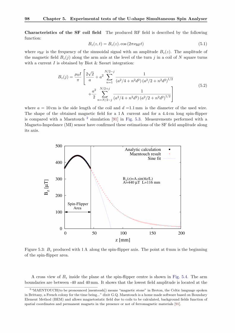
98 Chapter 5. Experimental tests of the U-shape Simultaneous Spin Analyser

Characteristics of the SF coil field The produced RF field is described by the following

function:

Bz(z, t) = Bz(z). cos (2πνRFt) (5.1)

where νRF is the frequency of the sinusoidal signal with an amplitude Bz(z). The amplitude of

the magnetic field Bz(j) along the arm axis at the level of the turn j in a coil of N square turns

with a current I is obtained by Biot & Savart integration:

Bz(j) =µ0I

π

2√2

a+ a2

N/2−j∑

n=1

1

(a2/4 + n2d2) (a2/2 + n2d2)1/2

+a2

2

N/2+j∑

n=N/2−j

1

(a2/4 + n2d2) (a2/2 + n2d2)1/2

(5.2)

where a = 10 cm is the side length of the coil and d =1.1mm is the diameter of the used wire.

The shape of the obtained magnetic field for a 1A current and for a 4.4 cm long spin-flipper

is compared with a Maentouch 2 simulation [91] in Fig. 5.3. Measurements performed with a

Magneto-Impedance (MI) sensor have confirmed these estimations of the SF field amplitude along

its axis.

0

100

200

300

400

500

0 50 100 150 200

Bz

[µT

]

z [mm]

Bz(z)=A.sin(πz/L)A=440 µT L=116 mm

Spin-FlipperArea

Analytic calculationMaentouch result

Sine fit

Figure 5.3: Bz produced with 1A along the spin-flipper axis. The point at 0mm is the beginning

of the spin-flipper area.

A cross view of Bz inside the plane at the spin-flipper centre is shown in Fig. 5.4. The arm

boundaries are between -40 and 40mm. It shows that the lowest field amplitude is located at the

2“MAENTOUCH(to be pronounced [mentoosh]) means “magnetic stone” in Breton, the Celtic language spoken

in Brittany, a French colony for the time being...” dixit G.Q. Maentouch is a home made software based on Boundary

Element Method (BEM) and allows magnetostatic field due to coils to be calculated, background fields function of

spatial coordinates and permanent magnets in the presence or not of ferromagnetic materials [91].

5.1. USSA design 99

centre of the SF. Thus, reference measurements are done at the centre of the spin-flipper in order

to determine the ability of the device to perform the spin-flip.

X (mm)

-40 -30 -20 -10 0 10 20 30 40

Y (

mm

)

-40

-30

-20

-10

0

10

20

30

40

380

400

420

440

460

480

500

520

540

T) vs X vs Y at Z = 0 mmµ(zB

Figure 5.4: Cross view of the RF magnetic field amplitude produced by 1A at the centre of the

spin-flipper from Maentouch [91]. Limits of the UCN guide are shown by the full black line.

The effective RF amplitude is obtained for an input signal at 6Vpp and 30 kHz and is of about

230/2 µT (the amplitude of the effective field contributing to the adiabatic spin-flip is half of the

linear oscillating field [92]) at the centre of the spin-flipper. This amplitude is large enough to

perform the adiabatic spin-flip, as presented in Fig. 5.7, showing the spin-flip probability obtained

as a function of the RF field amplitude by means of Eq (B.12) and the adiabaticity coefficient

given by Eq (B.10), according to the sine-cosine model [90].

Applicability of the sine-cosine model to USSA’s spin-flippers As shown in AppendixB,

particular field conditions, described by Eq (B.11), have to be fulfilled to perform the UCN adia-

batic spin-flip following the sine-cosine model. One of those conditions is that the field shape of

the RF field can be described by a sine. The analytic data set shown in Fig. 5.3 can be fitted using

a sine function and therefore the field shape of USSA’s spin-flippers fulfills the first condition to

apply the sine-cosine model. It will be shown later in 5.1.2.5 that the static field shape fulfills the

second condition to apply this model.

5.1.2.3 RF shielding

As described in the previous chapter, the principle of the simultaneous spin analysis is to detect

both spin states at the same time using one spin-flipper ON and the other OFF. It means that

100 Chapter 5. Experimental tests of the U-shape Simultaneous Spin Analyser

any RF magnetic field cross-talk between arms has to be removed.

From the existing literature about radio-frequency shielding (see [93]), one has to play with

the skin effect to remove the RF field coming from the active spin-flipper in the other arm. The

fraction of RF signal going through the material of thickness e around the RF field signal source is

e−e/δ where δ is the skin depth associated to the shielding material. The skin depth is expressed as

a function of the RF field frequency ν, the magnetic permeability µ and the electric conductivity

σ of the material:

δ =1√

πνµσ(5.3)

The main constraint in the USSA is that the opening of RF shielding around the UCN guiding

arms. Indeed, usual RF shielding surround the whole RF source or shielded antena. Copper has

been chosen because it is non magnetic and its electrical conductivity is high (σ = 5.96 × 107

S/m at 20C). The corresponding skin depth is much smaller than most materials: at 20-30 kHz,

the frequency range corresponding to the static field inside the spin-flipper, 0.8mm of copper is

sufficient (in theory) to attenuate 99% of the RF field. Therefore, a 1mm copper layer has been

placed around each USSA’s arm.

Experimental tests of the RF shielding For these tests, the spin-flip probability pSF within

the non-active arm is estimated through the adiabaticity parameter k (see AppendixB) calculated

from the RF magnetic field amplitude in the non-active arm Beff :

k =γnB2

eff

vminn ∂H0/∂z

pSF = 1− sin2 (π2

√1+k2)

1+k2

(5.4)

From yoke measurements, ∂H0

∂z is set to 0.15mT/cm (see 5.1.2.5). Because of the gravitational

boost below the nEDM spectrometer, the UCN energy at the spin-flipper level is at least 180 neV.

This is why the minimum speed vminn is set to 5m/s in order to be conservative.

The RF magnetic field measurements have been performed using an MI sensor from the In-

phynix company. RF shielding measurements have been performed on different planes along the

arm axis as shown in Fig. 5.5.

x=0

Active spin-flipperRF shielding

MI sensor

x

z

10 cm

Figure 5.5: RF shielding tests setup. The plane x=0 corresponds to the internal wall of the

non-active arm.

5.1. USSA design 101

Measurements in the non-active arm have been performed with a 30 kHz signal producing an

effective magnetic field amplitude at the centre of the active spin-flipper of 115 µT . Without

shielding, the maximal amplitude of the magnetic field in the non-active arm is about 7.5 µT

close to the internal wall as shown in Fig. 5.5 and Fig. 5.6.

0

1

2

3

4

5

6

7

8

-10 -5 0 5 10

Bz

[µT

]

z (with respect to the center of the SF) [cm]

x = 0 cmx = 2 cmx = 4 cmx = 6 cmx = 8 cm

With shielding

Figure 5.6: Bz amplitude along z in different x planes in the non-active spin-flipper without

shielding for diamond points. Lines are just used to guide eyes. The black dash line corresponds

to the highest measured amplitude with the RF shielding.

According to Eq (5.4), such a field amplitude leads to a spin-flip probability of about 1.9%,

which is obviously not satisfaying. Using the copper RF shielding, the maximal RF amplitude

has been decreased to less than 0.3 µT . The corresponding spin-flip probability is below the ppm

level as shown in Fig. 5.7.

In order to get such an RF magnetic field attenuation, the RF shielding end has been extended

by 5 cm above the spin-flipper. That is why the arm length has been increased by 5 cm with

respect to Geant4-UCN simulations and the quartz wedge is machined to let room for the RF

shielding. With such a shielding, the field amplitude inside the active arm is slightly decreased

down to 105 µT, which is enough to perform the spin-flip.

5.1.2.4 Analysing foils

The USSA analysing foils are made of a 25 µm aluminium substraste coated by a 400 nm iron

layer. These foils have been made at the PSI sputtering facility because the magnetic field required

(about 40mT) to reach the saturation is lower than other foils made in Caen or Mainz [94]. At

saturation, the theoretical magnetisation of the iron layer is about 2T. This corresponds to an

additional potential of ±120 neV according to the neutron spin state. The two analysers are made

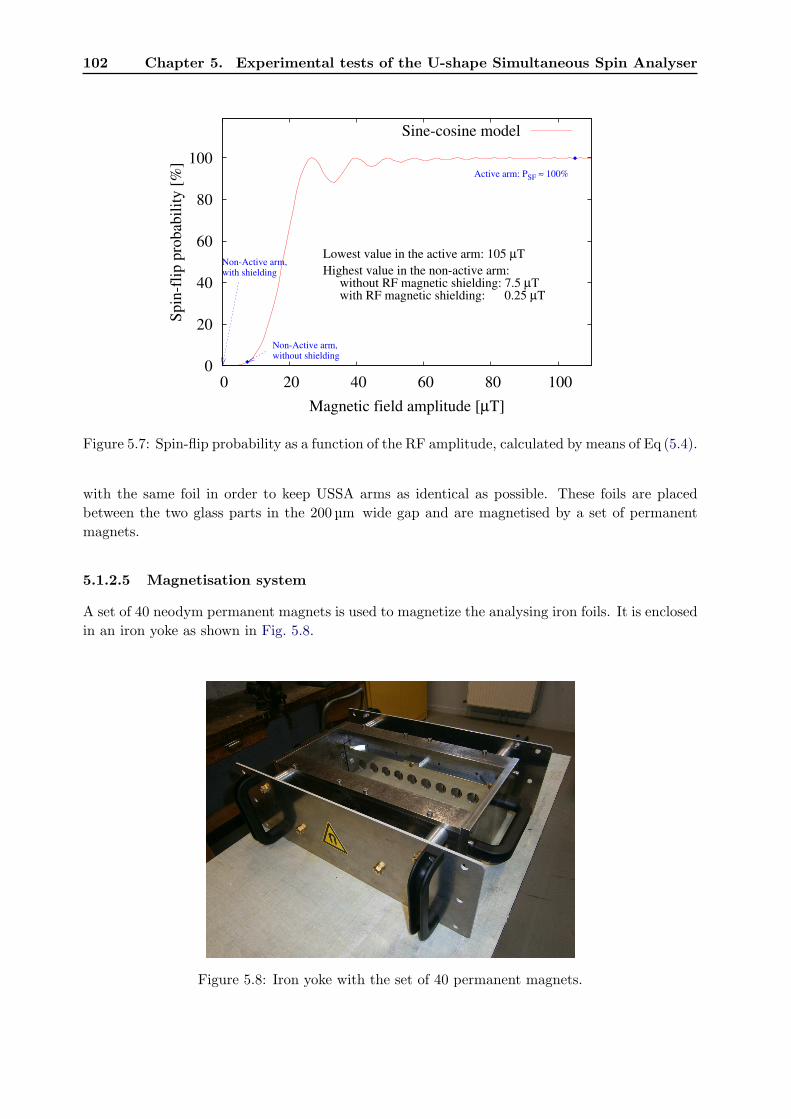
102 Chapter 5. Experimental tests of the U-shape Simultaneous Spin Analyser

0

20

40

60

80

100

0 20 40 60 80 100

Sp

in-f

lip

pro

bab

ilit

y [

%]

Magnetic field amplitude [µT]

Active arm: PSF ≈ 100%

Non-Active arm,without shielding

Non-Active arm,with shielding

Lowest value in the active arm: 105 µT

Highest value in the non-active arm: without RF magnetic shielding: 7.5 µTwith RF magnetic shielding: 0.25 µT

Sine-cosine model

Figure 5.7: Spin-flip probability as a function of the RF amplitude, calculated by means of Eq (5.4).

with the same foil in order to keep USSA arms as identical as possible. These foils are placed

between the two glass parts in the 200 µm wide gap and are magnetised by a set of permanent

magnets.

5.1.2.5 Magnetisation system

A set of 40 neodym permanent magnets is used to magnetize the analysing iron foils. It is enclosed

in an iron yoke as shown in Fig. 5.8.

Figure 5.8: Iron yoke with the set of 40 permanent magnets.

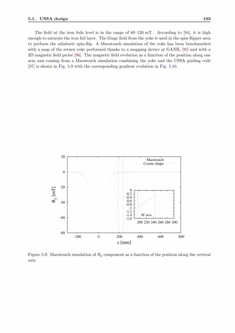
5.1. USSA design 103

The field at the iron foils level is in the range of 80–120 mT . According to [94], it is high

enough to saturate the iron foil layer. The fringe field from the yoke is used in the spin-flipper area

to perform the adiabatic spin-flip. A Maentouch simulation of the yoke has been benchmarked

with a map of the return yoke performed thanks to a mapping device at GANIL [95] and with a

3D magnetic field probe [96]. The magnetic field evolution as a function of the position along one

arm axis coming from a Maentouch simulation combining the yoke and the USSA guiding coils

[97] is shown in Fig. 5.9 with the corresponding gradient evolution in Fig. 5.10.

-80

-60

-40

-20

0

20

-200 0 200 400 600 800

By [

mT

]

z [mm]

MaentouchCosine shape

-1.6-1.4-1.2

-1-0.8-0.6-0.4-0.2

0

200 220 240 260 280 300

SF area

Figure 5.9: Maentouch simulation of By component as a function of the position along the vertical

axis.

104 Chapter 5. Experimental tests of the U-shape Simultaneous Spin Analyser

-10

-8

-6

-4

-2

0

2

4

6

8

10

-200 0 200 400 600 800

∂z

By [

mT

/cm

]

z [mm]

Maentouch

0 0.05

0.1 0.15

0.2 0.25

0.3 0.35

0.4 0.45

200 220 240 260 280 300

SF area

Figure 5.10: Maentouch simulation of By vertical gradient as a function of the position along the

vertical axis.

At the level of the spin-flipper centre, the gradient amounts to 0.15mT/cm and the transverse

field is in the range 0.05 – 0.8mT. The gradient value has been used to calculate a spin-flip

probability close to 100% in the ASF (see 5.1.2.3). In the spin-flipper area, it is also visible that

the field has approximately a cosine shape. This is the second field condition given by Eq (B.11)

to apply the sine-cosine model which is used to predict the spin-flip probability.

Besides, another important piece of information is the field value at the level of NANOSC

PMTs (Hamamatsu R11187). Even if those PMTs have a low sensitivity to high fields (Mumetal

shield around PMTs), a large magnetic field in the electron multiplication area would degrade or

even damage the PMTs. The field coming from the iron yoke is 0.7mT at 20 cm downstream. This

is low enough to allow a good working of NANOSC photomultipliers compared to the constructor

limit of 2mT.

5.1.3 Conclusions

The design and the assembly of each USSA’s part have been done in order to optimize the UCN

transmission and to handle the UCN spin as well as possible. Particularly, a lot of care has been

taken on the magnetic fields shape in order to get efficient spin-flippers and a spin holding field.

In the next section, performances tests of USSA’s subdevices are presented. These tests have been

carried out on the West-2 beam line at PSI.

5.2. USSA test on the West-2 beam line 105

5.2 USSA test on the West-2 beam line

After two weeks of preliminary tests at ILL3, performances of each USSA’s subsystem (spin-

flippers, analysing foils, guiding parts...) have been measured on the West-2 beam line at PSI

in order to demonstrate that the new spin analyser was ready to be installed below the nEDM

spectrometer.

5.2.1 Experimental setup

The experimental setup is shown in Fig. 5.11. UCNs come from the top, follow the bend and fall

down into the USSA. A stainless steel T-shaped guide was used between the bend and the USSA

in order to suppress the high energy component from the UCN energy spectrum. A magnetised

iron foil was used as a polariser right after the T-shaped guide. In order to carry out spin-flipper

efficiencies and analysing power measurements, a spin-flipper (#1) was placed below the polariser.

At the end of the line, a removable PMMA tube with a length of 27 cm was used in order to perform

measurements at two different heights. Thus, the distance D between the polariser and USSA’s

foils can be set either to 74 cm or to 101 cm.

52

120

30

27

44

NANOSC

USSA Analysers

Polariser

Bent guide

T guide

NiMo

Stainless Steel

Glass + NiMo

PMMA + NiMo

Glass + NiMo

Spin-flipper 1

USSA Spin-flippers

UCN shutter

UCNs

Beamline

USSA

Figure 5.11: West-2 beam line setup.

3Thanks to P. Geltenbort and Th. Brenner for the beam time and their warm welcome.

106 Chapter 5. Experimental tests of the U-shape Simultaneous Spin Analyser

5.2.2 Preliminary measurements

5.2.2.1 Background

During each proton kick, fast neutrons are produced and are detected by the USSA’s detectors.

Even though data recorded during the kick are not taken into account, the time shape of the

kick is not perfectly square as shown in Fig. 5.12. This time spectrum has been recorded with

the UCN shutter closed such as only fast neutrons coming from the source are detected. A small

amount of fast events is still produced 0.1 s after its end. In order to remove this contribution,

a set of 10 to 20 cycles with the UCN shutter closed is performed for each setup configuration.

The average number of fast events which occur right after the kick (normalised by the number

of detected UCNs on the West-1 beam line in a Cascade-U detector4) is then subtracted to the

detected UCN number for the runs of interest.

0 1 2 3 4 50

100

200

300

400

500

Time [s]

Neu

tro

n c

ou

nti

ng

rat

e [H

z]

Figure 5.12: Detected events in NANOSC-A during the 3 s proton kick.

5.2.2.2 Rough characterisation of the UCN energy spectrum

The lowest UCN energy (≃ 250 neV at USSA’s foils level) is calculated from the height difference

between the bottom of the West-2 beam line horizontal part and the USSA entrance. In order

to have an estimation of the fast UCN amount entering into the USSA, the polariser has been

replaced by a 100 µm aluminium foil with a NiMo coating and the USSA by a single NANOSC

detector. Measurements have been performed with and without the NiMo coated foil. Thus, the

UCN fraction with a larger energy than the NiMo Fermi potential is given by:

ε220 =Nw

Nw/o

(

1− pAlabs

) (5.5)

where Nw and Nw/o are respectively the detected UCN numbers with and without the NiMo

coated foil and pAlabs is the absorbed UCN fraction in the aluminium foil (∼ 30% [98]). The fast

UCNs fraction has been estimated to about 10%. It means that when the distance between the

NiMo coated foil and USSA’s foils is about 1m (lowest USSA height), the UCN fraction with

4Detector based on the neutron capture in a 10B layer and the GEM technology.

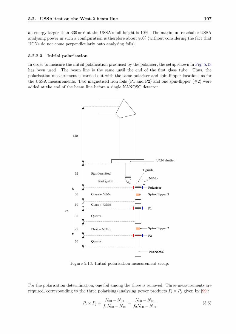
5.2. USSA test on the West-2 beam line 107

an energy larger than 330 neV at the USSA’s foil height is 10%. The maximum reachable USSA

analysing power in such a configuration is therefore about 80% (without considering the fact that

UCNs do not come perpendicularly onto analysing foils).

5.2.2.3 Initial polarisation

In order to measure the initial polarisation produced by the polariser, the setup shown in Fig. 5.13

has been used. The beam line is the same until the end of the first glass tube. Thus, the

polarisation measurement is carried out with the same polariser and spin-flipper locations as for

the USSA measurements. Two magnetised iron foils (P1 and P2) and one spin-flipper (#2) were

added at the end of the beam line before a single NANOSC detector.

52

120

30

NANOSC

Bent guide

T guide

NiMo

Stainless Steel

Glass + NiMo

UCN shutter

Plexi + NiMo27

Glass + NiMo

Quartz

Quartz

Polariser

P1

P2

Spin-flipper 1

Spin-flipper 2

10

30

30

97

Figure 5.13: Initial polarisation measurement setup.

For the polarisation determination, one foil among the three is removed. Three measurements are

required, corresponding to the three polarising/analysing power products Pi × Pj given by [99]:

Pi × Pj =N00 −N01

f1N00 −N10=

N00 −N10

f2N00 −N01(5.6)

108 Chapter 5. Experimental tests of the U-shape Simultaneous Spin Analyser

where Pi/j is the polarising/analysing power of foils i/j, f1/2 is the spin-flipper efficiency of spin-

flipper 1/2. N12 indices are the SF1 and SF2 states: 0 for SF OFF and 1 for SF ON. The SF

efficiencies f1 and f2 are obtained using only the polariser and the last foil. The results are:

f1 =N11 −N01

N00 −N10= 96.1± 4.6% (5.7)

f2 =N11 −N10

N00 −N01= 99.3± 4.8% (5.8)

The three measured polarising/analysing power products are:

P × P1 = 41.0± 1.5% P × P2 = 46.2± 1.9% P1 × P2 = 38.0± 1.3%

The initial polarisation P is deduced from those measurements:

P =

√

P × P1.P × P2

P1 × P2= 70.6± 3.2% (5.9)

5.2.3 Tests with unpolarised UCNs

5.2.3.1 Arm detection asymmetry

The USSA has to symmetrically detect spin up and spin down UCNs. In order to check such a

behaviour, the USSA detection asymmetry between arms A and B, (NA − NB)/(NA + NB) has

been measured. For such a purpose, the polariser and USSA’s analysing foils are removed. The

neutron counting rates for arms A and B and asymmetry are shown in Fig. 5.14. The average

asymmetry between arms A and B is 0.43± 0.07%. It combines different arm transmissions and

the two NANOSCs different detection efficiencies. The conclusion is that the arms detection is

nearly symmetrical.

0

100

200

300

400

500

600

700

Neu

tro

n c

ou

nti

ng

rat

e [H

z]A

sym

met

ry

0 10 20 30 40 50

-10

-5

0

5

10

Time [s]

[%]

Arm AArm B

A=0.43(7)%

Figure 5.14: Detection asymmetry and neutron counting rates as a function of the detection time.

Another measurement was carried out with the two USSA’s analysers in order to know whether

the analysing foils have the same UCN transmission. There is no polariser in the apparatus and

all spin-flippers are turned OFF. The average asymmetry is A = 0.40± 0.11% (χ2 = 0.96). This

asymmetry is consistent with the previous detection asymmetry. It means that USSA’s foils do

not introduce any additional asymmetry.

5.2. USSA test on the West-2 beam line 109

5.2.3.2 USSA transmission

Transmission measurements were performed using a single NANOSC detector and then the USSA

at the same location on the beam line. The transmission is defined as the ratio between the

number of detected neutrons with the USSA and a single NANOSC detector. These numbers

were normalised with the number of detected neutrons simultaneously measured on the West-1

beam line by a Cascade-U detector. The worst transmission, T = 80.8 ± 0.6% was obtained for

the lowest position (D = 105 cm), hence for the largest distance between the polariser and USSA

foils. For the shortest distance (D = 75 cm), a transmission of 83.2± 0.7% was measured. This is

an indication that one needs a higher Fermi potential in the USSA in order to increase its UCN

transmission.

5.2.3.3 Fraction of detected UCNs after reflection in the other arm

In order to measure the probability for a UCN to be reflected on an analysing foil and then to be

detected in the other arm, the two configurations of the Fig. 5.15 were used.

P=0% P=0%

Figure 5.15: USSA configurations used to determine the reflection probability from the wrong

spin detection arm to the good one on the West-2 beam line. In one case there is no foil. In the

other case, a single analysing foil is added.

For both configurations, N0 unpolarised UCNs fall down into the USSA. The difference between

the two configurations is the presence of a single analysing foil in one of the two USSA arms.

During the measurement with no foil, the number of detected UCNs is the same in both arms:

NA ≃ NB =N0

2(5.10)

In the second case, roughly N0/4 UCNs are going through the analysing foil in arm A. The UCN

fraction absorbed inside the analyser is εabs and the probability for a UCN to be reflected on

the analyser to the other arm is pref . Assuming negligible losses per reflection on the analysers,

numbers of detected UCNs in arms A and B are:

N ′A = N0

4 (1− εabs)

N ′B = N0

2 + N0

4 pref(5.11)

110 Chapter 5. Experimental tests of the U-shape Simultaneous Spin Analyser

Using Eq (5.10) and Eq (5.11) the reflection probability pref and the UCN absorption fraction εabsare finally determined as:

pref =2N ′

BNB

− 2 = 33.6± 3.1%

εabs = 1− 2N ′A

NA= 2.7± 1.3%

(5.12)

The UCN fraction absorbed inside the analysing foil, 2.7±1.3%, is of the same order of magnitude

as the calculated UCN attenuation in a 25 µm aluminium foil. The probability for a neutron to be

reflected from one arm to the other amounts to 33.6± 3.1%. It is much lower than the calculated

value from Geant4-UCN simulations of 84% (see 4.6.2). This can be partly explained by the

fact that UCNs reflected upstream go back into the UCN tank and can hardly come back to

the USSA. In addition, UCN simulations were made with a perfect coating and glass structure,

without slits which overestimate the number of UCNs able to go to the other arm.

5.2.4 Tests with polarised neutrons

5.2.4.1 Spin-flippers efficiencies

Spin-flippers efficiencies measurements were carried out with the polariser using a single foil located

in the arm where the spin-flipper is characterised. This has been done in order to avoid multiple

passages between the two arms. In such a case, since the number of passages is not known, it is

not possible to use the transmission matrices formalism defined in [99]. Spin-flippers efficiencies

have been measured using Eq (5.8): fA = 97.0 ± 1.2% and fB = 97.1 ± 0.9%. These efficiencies

do not change with the height of the USSA with respect to the horizontal beam line. It means

that USSA’s spin-flippers can handle quite fast UCNs without efficiency loss. However, USSA’s

spin-flippers are not fully efficient. Two explanations are possible. The first one would be the

existence of a non-adiabatic area in the spin-flippers. The other one could be multiple passages

through the active SF and multiple reflections on the USSA analyzer. In that case, the effect

would be to depolarise UCNs and thus allow their passage through the analysing foil. As a result,

it would lower the effective spin-flipper efficiency.

5.2.4.2 RF cross-talk measurements

Possible RF cross-talk between the two arms was studied. For these tests, a single foil was used in

the non-active arm (SF OFF). The number of detected UCNs in the non-active arm is measured

when the spin-flipper of the active arm is turned ON or OFF. No change has been observed. The

relative deviation NOFF−NON

NOFFis equal to 0.15±0.62%. The conclusion is that there is no cross-talk

between USSA’s arms.

5.2.4.3 Analysing power of the USSA’s foils

Measurements of the spin analysing power of the USSA’s foils have been carried out using two

different methods. First, the measurements devoted to the spin-flippers efficiencies determination

have been used to find the analysing power of the active arm foil. Second, both foils stayed in the

USSA and the effective spin analysing power of the USSA have been measured.

With a single analysing foil: Analysing power measurements performed with a single foil in

the USSA are summarised in Tab. 5.1. For the shortest distance, the analysing powers of both foils

are the same, which shows that the analysing foil spin treatment is similarly performed in each

arm. The analysing power difference (about 15%) between the two height setup configurations

can be explained using the NiMo foil transmission results (see 5.2.2.2). Indeed, with the lowest

5.2. USSA test on the West-2 beam line 111

Polariser→USSA foils D = 74 cm D = 101 cm

PA [%] 91.0± 3.4 77.4± 1.7

PB [%] 89.7± 2.7 Not measured

Table 5.1: Single foil analysing powers measurements.

USSA height setup (D = 101 cm), the fast UCN fraction is larger. As a result, the UCN fraction

that USSA’s foils are not able to analyse is larger and the USSA spin analysing power is lowered.

With two analysing foils: The USSA analysing power measurements are shown in Tab. 5.2.

Polariser→USSA foils D = 74 cm D = 101 cm

PUSSA [%] 83.5± 2.5 77.3± 2.8

Table 5.2: USSA analysing power measurements.

For D = 74 cm, the analysing power is different by about 6% from a single foil to two foils.

This is not the case for the setup with D = 101 cm. This is not expected since the spin analysing

power should be lower with the two USSA foils. Indeed, because of bounces from one arm to the

other on analysing foils and crossings of the SF, one expects to observe more depolarisations with

the two foils in the USSA.

5.2.5 Conclusions

Similar efficiencies of 97% were measured for both spin-flippers A and B. The deviation due

to a possible cross-talk between the two arms was measured at 0.15 ± 0.62% and cross-talk is

thus excluded below the percent level. The analysing powers of USSA foils have been measured

to 91.0 ± 3.4% and 89.7 ± 2.7%. It shows that USSA foils analyse the spin symmetrically. In

addition, the arm detection asymmetry has been estimated to 0.43 ± 0.07% in transmission and

0.40 ± 0.11% with the two analysers in the USSA. It confirms the symmetry between the two

arms.

The USSA analysing power was measured to be about 80%. It is lower than with a single

analysing foil by about 6%. A possible explanation would be the multiple bounces onto the

analysing foils and passages through the active spin-flipper which could lead to UCN depolarisa-

tions. The USSA transmission was measured to 80% for the highest energy conditions. It could

be further improved by replacing the current NiMo coating by diamond or 58NiMo coatings which

are known to have larger Fermi potentials (> 280 neV).

Measurements performed with the USSA on the West-2 beam line showed that all USSA’s

subsystems work properly and that the USSA symmetrically treat the two UCN spin states. As

a result, the USSA was installed below the nEDM experiment to be tested as described in the

next section. Below the nEDM spectrometer, USSA performances are expected to be better than

below the West-2 beam line because of a softer UCN energy spectrum.

112 Chapter 5. Experimental tests of the U-shape Simultaneous Spin Analyser

5.3 USSA test below the oILL spectrometer

In order to measure the possible nEDM statistical sensitivity improvement with respect to the

sequential system, the USSA was integrated in the nEDM apparatus. A drawing of the setup is

shown in Fig. 5.16. The distance between the precession chamber centre and the USSA analysing

foils is about 2.1m. It means that the UCN energy is gravitationally boosted by 210 neV at the

foil location. The USSA hangs on an aluminium plate below the switch box and is also maintained

by an external aluminium profile structure fixed in the concrete floor below the thermohouse. One

pair of additional guiding coils have been added between the switch and the USSA in order to

maintain the UCN polarisation.

Wooden floor

Concrete floor

Mechanical

structure

USSA

Switch box

Precession

chamber

42.5

37.5

126

Figure 5.16: USSA integration drawing in the nEDM apparatus. Dimensions are in cm.

5.3. USSA test below the oILL spectrometer 113

The UCNs detected in the Cascade-U detector on the West-1 beam line were used for the mon-

itoring. It allowed one to take care of UCN source fluctuations in order to compare measurements

performed with the USSA and the sequential system. An important difference between the two

systems is the analysing foils height: they are 40 cm lower in the USSA. Three types of runs have

been performed: direct mode, T1 measurement and EDM run. The guiding field configuration did

not change for the sake of the comparison.

5.3.1 Direct mode measurements

In direct mode, polarised UCNs coming from the horizontal guide are directly going into the

USSA. With such a configuration, the USSA asymmetry was found to be 77.35 ± 0.16%. The

analysing power of the sequential system was estimated with the upstream spin-flipper during

2013, a few months before the USSA installation. The measured asymmetry was 83.83 ± 0.35%

i.e. larger than with the USSA. The lower USSA spin analysis efficiency can be partly explained

(at the 2% level) by a fast UCN component visible in the arm B in Fig. 5.17 at the beginning of

the counting rate distribution between 3 and 6 s. These fast UCNs are able to cross the USSA’s

analysers whatever their polarisation and thus decrease the asymmetry. Once they are detected,

the USSA asymmetry saturates at 79%. Additional possible explanations for the lower USSA

analysing power with respect to the sequential system could be a bad guiding field along the UCN

path or a lower foil ability to analyse the UCN spin, either due to the foil itself or to the foil

height difference in the two setups. The last possible explanation is that depolarisations occuring

in the USSA (because of multiple foil reflections) could decrease the effective analysing power of

the system (see 5.2.4.3).

Arm A: SF OFF

Arm B: SF ON

Instantaneous asymmetry

Arm A: SF OFF

Arm B: SF ON

Instantaneous Asymmetry

Time [s]

Neu

tro

n c

ou

nti

ng

rat

e [c

ou

nts

/s] 12000

10000

8000

6000

4000

2000

0

12000

10000

8000

6000

4000

2000

03 4 5 6 7 8 9 10

Asy

mm

etry

[%

]

100

80

60

40

20

0

100

80

60

40

20

0

0 20 40 60 80 100 120 140 160 180 200

Fast UCNs

3 4 5 6 7 8 9 10

Figure 5.17: UCN counting rates (arms A and B) and asymmetry as a function of the emptying

time in direct mode.

114 Chapter 5. Experimental tests of the U-shape Simultaneous Spin Analyser

5.3.2 T1 measurements comparison

T1 measurements are performed in order to estimate the longitudinal relaxation time T1. In this

case, it is used to study the influence of the UCN storage on the spin analysing power of the USSA

and to compare USSA performances with respect to the sequential sytem. In this kind of run,

the precession chamber is filled by UCNs during 30 s, then UCNs are stored during a time T and

finally counted during 50 s. The asymmetry as a function of the storage time is shown in Fig. 5.18

for both the USSA and the sequential system.

66

68

70

72

74

76

78

0 50 100 150 200 250

Asy

mm

etry

[%

]

Storage time T [s]

USSASequential

USSA: τfast + T1 fit

Sequential: T1 fit [40:210 s]

Figure 5.18: Asymmetry as a function of storage time for the USSA (red cross) and the sequential

system (blue star) during T1 measurement. The black dashed line corresponds to the USSA data

fit using Eq (5.19). The blue dash line corresponds to the usual T1 fit applied to the sequential

analyser data between 40 and 210 s.

With the USSA, a maximum is visible around T = 50 s and then the T1 exponential decrease is

observed for larger storage times. This maximum is thought to arise from a fast UCN component.

An attempt to model the phenomenon has been carried out hereafter.

The UCN spin populations as a function of the storage time are described by:

dN↑

dT = 1τflip

(N↓ −N↑)− N↑

τloss= 1

2T1(N↓ −N↑)− N↑

τlossdN↓

dT = 1τflip

(N↑ −N↓)− N↓

τloss= 1

2T1(N↑ −N↓)− N↓

τloss

(5.13)

where N↑/↓ are respectively the number of spin up/down UCNs stored in the precession chamber

at a given time T , T1 is the longitudinal relaxation time and τloss the time constant associated to

wall losses and the beta decay.

Solving (5.13) for a neutron population with an initial polarisation P0 gives:

N↑(T ) =N0

2 e−T/τloss[

1 + P0e−T/T1

]

N↓(T ) =N0

2 e−T/τloss[

1− P0e−T/T1

] (5.14)

5.3. USSA test below the oILL spectrometer 115

where N0 is the initial number of UCNs inside the precession chamber.

In order to take into account the energy loss dependence, the number of stored UCNs can be

described with two time constants:

N(T ) = N slow0 e−T/τslow +N fast

0 e−T/τfast (5.15)

τslow is assigned to UCNs with low energies compared to the wall Fermi potential and τfast is

assigned to UCNs with higher energies. The number of detected UCNs as a function of the

storage time is shown in Fig. 5.19. One gets: τslow = 210 ± 15 s and τfast = 59.0 ± 8.7 s. Using

such an energy partition, the UCN population can be split as followed:

N↑(T ) =N0

2

[

1 + P0e−T/T1

] [

(1− pfast)e−T/τslow + pfaste

−T/τfast]

N↓(T ) =N0

2

[

1− P0e−T/T1

] [

(1− pfast)e−T/τslow + pfaste

−T/τfast] (5.16)

where pfast is the initial proportion of fast UCNs.

The UCN population called “fast” has an energy comparable or larger than the Fermi potential

of the DPS in the chamber, around 160 neV. This energy is close to the limit that analysing foils

can handle (330 neV in theory i.e. about 130 neV in the precession chamber). Because the fastest

UCNs are too energetic to be analysed by USSA’s foils, the number of fast UCNs detected in each

arm is the same:

N fastA (T ) = N fast

B (T ) =N fast

tot (T )

2=

N0

2pfaste

−T/τfast (5.17)

Thus, the USSA asymmetry is described by:

A(T ) =NA −NB

NA +NB=

N slow↑ (T )−N slow

↓ (T )

N slow↑ (T ) +N slow

↓ (T ) +N fasttot (T )

(5.18)

=P0e

−T/T1

1 + pfast1−pfast

e−T (1/τfast−1/τslow)(5.19)

Using τfast and τslow extracted from (5.15) as inputs, the fit of the USSA data with the function

(5.19) gives the following parameters (χ2 = 0.63):

P0 = 79.4(9)% T1 = 1930(90) s pfast = 6.8± 1.3%

The P0 and T1 values are of the same order of magnitude as previous measurements performed

over the year 2013 (e.g. P0 = 72.2± 5.5%, T1 = 2090± 210 s). The proportion of fast UCNs not

analysed by iron foils is consistent with MCUCN simulations results [100] which gives an initial

UCN fraction with energies higher than 130 neV in the precession chamber (i.e. corresponding

to 330 neV at USSA foils level) of a few percents. It has to be precised that the “slow” and

“fast” components do not correspond here to well defined parts of the UCN spectrum. Therefore,

quantitative results of this model have nonetheless to be taken with care. Finally, the asymmetry

decrease due to the fast component is found to be negligible for storage times above 150 s, i.e. for

typical EDM storage times. In that case, the low USSA height has therefore no influence on the

USSA spin analysing power.

With the sequential system, a larger asymmetry is observed for T < 50 s. It is likely due to

the fast UCN component which go through the analyser, whatever the UCN spin state. As the

sequence starts with the most populated spin state for this set of measurements, this spin state

population is overestimated and thus the corresponding asymmetry.

The most interesting measurements for the comparison between the USSA and the sequential

system are above 150 s i.e. for typical storage times in the nEDM experiment. The polarisation

and the number of detected UCN are summarised in Tab. 5.3 for a storage time T = 180 s. During

the USSA measurements, there was no monitoring recorded on West-1. The monitored UCN count

has been therefore extrapolated from measurements surrounding this measurement within a day.

116 Chapter 5. Experimental tests of the U-shape Simultaneous Spin Analyser

A [%] Ntot NWest-1

USSA 71.9(3) 4160(30) 2.07(5)×106 (extrapolated)

Sequential 68.5(8) 3020(45) 1.700(13)×106

Ratio 1.050(13) 1.131(33)

Table 5.3: Asymmetry A and total number of detected UCNs Ntot for the USSA and the sequential

analyser with a storage time of 180 s. NWest-1 is the monitored UCN counts on the West-1 beam

line. The ratio of the total number of detected UCNs is calculated with the number of detected

UCNs normalised with NWest-1.

0

2000

4000

6000

8000

10000

12000

14000

16000

0 50 100 150 200 250

UC

N c

ounts

[#]

Storage time T [s]

USSA: exp. dataUSSA: fit

Sequential: exp. dataSequential: fit

Norm

ali

sed

Figure 5.19: Number of detected UCNs as a function of the storage time inside the precession

chamber. Dash lines correspond to USSA and sequential system data fits using (5.15).

As visible in Fig. 5.18, the UCN polarisation measured with the USSA is larger than the one

with the sequential analyser by about 5% for T = 180 s. Besides, the number of detected UCNs

is also larger using the USSA by 13%, as shown in Fig. 5.19. The statistical improvement coming

from the USSA with respect to the sequential system is estimated through the variable A√N and

amounts for 11.6± 3.7%.

5.3.3 Detected UCNs fraction after reflection in the other arm

In order to measure the probability for UCN to be reflected from one arm and then detected in

the other arm, the configurations of the Fig. 5.20 have been used.

For both configurations, N0 unpolarised UCNs fall down on the USSA after 50 s of storage time.

The only difference between the two configurations is the presence of a single analysing foil located

5.3. USSA test below the oILL spectrometer 117

P=0% P=0%

Figure 5.20: USSA configurations used to determine the reflection probability from the wrong

spin detection arm to the right one. In one case, the two analysing foils are installed. In the other

case, one foil is removed.

in one of the two USSA arms. With two foils, the number of detected neutrons is the same in

both arms:

NA = NB =N0

4(1− εabs) (1 + pref) (5.20)

where εabs and pref have been already defined in 5.2.3.3.

With a single foil, less UCNs are detected in the arm A because they are not reflected from

the arm B. Thus, numbers of detected UCNs in arms A and B in that case are:

N ′A = N0

4 (1− εabs)

N ′B = N0

2

(

1 + pref2

) (5.21)

Using Eq (5.20) and (5.21) the reflection probability pref and the UCN absorption fraction εabsare finally determined:

pref =NAN ′

A− 1 = 52.8± 2.8%

εabs = 1− N ′A

N ′B(2 + pref) = 5.8± 1.5%

(5.22)

The UCN fraction absorbed in the aluminium foil substrate is twice larger than the one measured

on the West-2 beam line (2.7±1.3%). It might be due to the UCN energy spectrum difference

between the two setups. Indeed, UCNs are more energetic on the West-2 beam line. As the

absorption cross section varies proportionally to 1/vn, the proportion of absorbed UCNs in the

aluminium is larger.

The second point is that the fraction of reflected UCNs from one arm to the other (52%) is

larger on the EDM line than on West-2 (about 34%). This may be explained by the fact that a

part of reflected UCNs on West-2 can be lost afterwards, as the West-2 beam line is open towards

the UCN tank. On the contrary, during the emptying below the nEDM spectrometer, UCNs can

be stored between the chamber and the USSA. Thus, UCNs can go upwards to the chamber and

fall back into the USSA where they may be detected.

118 Chapter 5. Experimental tests of the U-shape Simultaneous Spin Analyser

5.3.4 EDM run type comparison

The last comparison between the USSA and the sequential system has been performed for usual

nEDM runs. The Ramsey central fringe fitting using normalised N↑ and N↓ is shown in Fig. 5.21.

The normalisation is performed with the number of UCNs recorded in the monitoring position.

The average number of UCN counts is almost symmetric and both visibilities α↑ and α↓ are

consistent. This shows that both spin states are symmetrically treated in the USSA.

[Hz]RF - fHg

γ/Hg

.fn

γ f = ∆-0.0015 -0.001 -0.0005 0 0.0005 0.001 0.0015

Norm

aliz

ed N

eutr

on C

ounts

1200

1400

1600

1800

2000

2200

2400

2600

/ ndf 2χ 18.28 / 17

Prob 0.3715

avg

upN 10.09± 1932

avgup

α 0.02511± 0.6157

avg

upφ 0.01516± -0.295

/ ndf 2χ 18.28 / 17

Prob 0.3715

avg

upN 10.09± 1932

avgup

α 0.02511± 0.6157

avg

upφ 0.01516± -0.295

/ ndf 2χ 19.47 / 17

Prob 0.3021

avgdown

N 9.722± 1859

avgdownα 0.0273± 0.6521

avg

downφ 0.01441± -0.281

/ ndf 2χ 19.47 / 17

Prob 0.3021

avgdown

N 9.722± 1859

avgdownα 0.0273± 0.6521

avg

downφ 0.01441± -0.281

Figure 5.21: First Ramsey pattern taken with the USSA (in B0 up configuration).

α [%] Ntot NWest-1

USSA 63.4(18) 3791(14) 1.878(5) ×106

Sequential 59.7(22) 2692(15) 1.651(16) ×106

Ratio 1.062(49) 1.239(10)

Table 5.4: Visibility α and total number of detected UCNs measured with the USSA and the

sequential analyser for EDM runs. NWest-1 is the number of detected UCNs on the West-1 beam

line. The UCN ratio is calculated with the number of detected UCNs normalised with NWest-1.

The comparison between the USSA and the sequential system is summarised in Tab. 5.4. With

the USSA, both the visibility and the number of detected UCNs are larger than with the sequential

system. This is consistent with results coming from T1 measurements. However, the statistical

error on the visibility is large, because of the rather low number of cycles (20). The improvement

of the EDM sensitivity is estimated through the variable α√N and amounts for 18.2± 6.1%. The

largest contribution on this improvement is coming from the larger number of detected UCNs.

5.3. USSA test below the oILL spectrometer 119

5.3.5 Conclusions

In direct mode, the USSA analysing power is smaller than the analysing power of the sequential

system by about 6.5%. This may be explained by the lower height of USSA analysing foils with

respect to the sequential system analysing foils (25 cm lower). However, in case UCNs are stored,

the USSA spin analysis efficiency is not decreased for storage times larger than 150 s, due to the

UCN spectrum softening in the precession chamber. For measurements carried out with such

storage times and UCN energy conditions, the USSA asymmetry is larger than the sequential one

by 2-3%.

From nEDM runs, the visibility and the UCN counts are respectively increased by 6.2 ±4.9% and by 23.9± 1.0% with the USSA. This leads to an improvement of the nEDM statistical

sensitivity of 18.2±6.1% with respect to the sequential analysis. In addition, the spin treatment is

almost symmetric. During preliminary measurements performed at ILL, the NANOSC detection

efficiencies have been measured to be different by 1.1 ± 0.4% and the arms transmissions by

0.5 ± 1.5%. On the West-2 beam line, the asymmetry for unpolarised UCNs has been measured

to 0.4% in transmission (without analysing foils). When USSA foils are added, no change is

measured. In addition, their analysing powers are of the order of 90% and are equal. Spin-flippers

efficiencies have also been measured and are equal (97%), without influencing the non-active arm.

Since the USSA has shown better performances than the sequential system, with a spin treatment

almost symmetric, it is now part of the nEDM apparatus.

Finally, the USSA design with Geant4-UCN and its building have succeeded in the produc-

tion of a new simultaneous spin analyser, able to symmetrically treat the two spin components

and also to increase the UCN statistics.

In order to further improve the UCN statistics, the NiMo coating (VF = 220 neV) could be

replaced by diamond or 58NiMo coatings which have a theoretical Fermi potential around 300 neV.

The Fermi potential of a diamond coating over a quartz substrate has been measured by means

of cold neutron reflectometry on the NARZISS 5 instrument at PSI to be about 305 neV and loss

per bounce measurements are planned to be studied on the West-1 beam line. But the first USSA

upgrade will be performed with 58NiMo. The coating will be performed either at PSI on the

sputtering device or at LPC with the evaporator. Tests are planned for Autumn 2014 or in 2015.

5Test instrument for neutron optical devices.

Chapter 6

nEDM data analysis

Contents

6.1 The neutron frequency extraction . . . . . . . . . . . . . . . . . . . . . . . 123

6.1.1 Cycle definition . . . . . . . . . . . . . . . . . . . . . . . . . . . . . . . . . . . 123

6.1.2 Principle . . . . . . . . . . . . . . . . . . . . . . . . . . . . . . . . . . . . . . 124

6.1.3 Alternative method . . . . . . . . . . . . . . . . . . . . . . . . . . . . . . . . 125

6.2 Raw data selection . . . . . . . . . . . . . . . . . . . . . . . . . . . . . . . . . 127

6.2.1 Offline analysis of the detected UCN number . . . . . . . . . . . . . . . . . . 127

6.2.2 Other cuts . . . . . . . . . . . . . . . . . . . . . . . . . . . . . . . . . . . . . 127

6.2.3 Cuts effects on the χ2 of the Ramsey central fringe fit . . . . . . . . . . . . . 128

6.3 Hg frequency extraction . . . . . . . . . . . . . . . . . . . . . . . . . . . . . 129

6.3.1 Effect of the Hg frequency estimator on the neutron frequency fit . . . . . . . 131

6.4 Effect of gradient variations on the neutron Larmor frequency fit . . . . 132

6.5 Study of the neutron Larmor frequency precision . . . . . . . . . . . . . . 134

6.6 R auto-correlation . . . . . . . . . . . . . . . . . . . . . . . . . . . . . . . . . 135

6.7 Study of the neutron Larmor frequency extraction with simulated data 136

6.7.1 Data production . . . . . . . . . . . . . . . . . . . . . . . . . . . . . . . . . . 136

6.7.2 Ideal conditions . . . . . . . . . . . . . . . . . . . . . . . . . . . . . . . . . . . 137

6.7.3 B field fluctuations . . . . . . . . . . . . . . . . . . . . . . . . . . . . . . . . . 137

6.7.4 UCN source production decay . . . . . . . . . . . . . . . . . . . . . . . . . . . 138

6.7.5 Static magnetic field gradient . . . . . . . . . . . . . . . . . . . . . . . . . . . 138

6.7.6 Daily variation of the magnetic field gradient . . . . . . . . . . . . . . . . . . 138

6.7.6.1 Effect of a daily gradient variation on the χ2 . . . . . . . . . . . . . 139

6.7.7 Relevance of the δ term use . . . . . . . . . . . . . . . . . . . . . . . . . . . . 140

6.7.8 Conclusions on the neutron frequency extraction . . . . . . . . . . . . . . . . 140

6.8 nEDM measurement with 2013 data . . . . . . . . . . . . . . . . . . . . . . 141

6.8.1 Systematic errors . . . . . . . . . . . . . . . . . . . . . . . . . . . . . . . . . . 141

6.8.1.1 Geometric Phase Effect (GPE) . . . . . . . . . . . . . . . . . . . . . 142

6.8.1.2 Quadrupole difference . . . . . . . . . . . . . . . . . . . . . . . . . . 143

6.8.1.3 Uncompensated B-Drifts . . . . . . . . . . . . . . . . . . . . . . . . 144

6.8.2 Raw nEDM extraction . . . . . . . . . . . . . . . . . . . . . . . . . . . . . . . 144

6.8.3 Correction of the Earth’s rotation frequency shift . . . . . . . . . . . . . . . . 146

6.8.4 Suppression of the geometric phase effect . . . . . . . . . . . . . . . . . . . . 147

6.9 Conclusion . . . . . . . . . . . . . . . . . . . . . . . . . . . . . . . . . . . . . 148

6.1. The neutron frequency extraction 123

In the nEDM collaboration, two groups independently analyse the nEDM data: the French

group (LPC, LPSC and CSNSM) and the PSI group. This chapter presents the analysis performed

by the French team with the 2013 PSI data. The basics of the neutron Electric Dipole Moment

measurement has been already described in 2.2.1. A previous analysis, performed by the PSI team

on 2012 data is presented in [56].

The 2013 data set was collected in August. Even if only 13 runs have been recorded, some

of them are particularly long (three days for the longest one) and the key parameters for a low

nEDM sensitivity were rather good. The precession time was set to 180 s with an applied electric

field of 10 kV/cm in average. With such a storage time, the final visibility was close to 60% and

the number of mean detected UCNs per cycle was 6650. Using Eq (2.17), the expected nEDM

sensitivity per cycle should be close to 4 × 10−24 e.cm. In total, about 2900 cycles have been

recorded during this month, leading to an expected integrated sensitivity of about 8× 10−26 e.cm

for the 2013 data set.

The first part explains how the neutron frequency is recovered with either neutron counts or

with the asymmetry. Furthermore, a study of the raw data selection before the main analysis

is performed. Then, the effect of different methods to estimate the Hg precession frequency is

studied. Then, a study of the neutron frequency extraction procedure is presented, using either

experimental data or simulated one. Finally, results of the 2013 nEDM data campaign will be

presented, summarising the systematic errors budget and the current nEDM sensitivity of the

experiment.

6.1 The neutron frequency extraction

The neutron Larmor frequency is measured via the Ramsey separated oscillating fields method.

The principle of the extraction – as it was performed in the previous stage of the nEDM experiment

[101] – is described in section Sec. 2.2 and in the following section. An alternative method is

described in section 6.1.3.

6.1.1 Cycle definition

Time [s]0 50 100 150 200 250 300

10

210

310

410

Not counted UCNs

Monitored UCNs

Spin up

Spin down

Neu

tro

n c

ou

nti

ng

rat

e [c

ou

nts

/s]

Monitoring

Up

Down

Filling

Figure 6.1: Neutron counting rate as a function of the detection time. Colours indicate different

periods of detection given by the main acquisition: monitor (mauve), spin up (red) and spin down

neutrons (blue). The peak visible before the first spin up detection period (t ≃ 220 s) does not

correspond to physical events.

124 Chapter 6. nEDM data analysis

A measurement of the neutron Larmor frequency is performed every cycle. A cycle lasts 6min

and defines the following sequence, as illustrated in Fig. 6.1.

First, the precession chamber is filled for about 30 s. Then, the switch moves to the monitoring

position and the remaining UCNs located in guides and the UCN tank are directly going to the

UCN detector. This number of neutron counts is used to normalise the number of detected UCNs

at the end of each cycle. In the mean time, UCNs are stored during 180 s and the Ramsey method

is applied. Finally, the UCN shutter is open and UCNs directly fall downwards to the detector.

During this period, UCNs are sequentially detected.

During a typical run, about 100 - 200 cycles are collected, with regular electric field polarity

changes, according to the following pattern: -0++0–0+... with 12 cycles for both positive and

negative polarities and only 6 cycles without electric field.

6.1.2 Principle

During nEDM measurements, one works around the resonance where the Ramsey curve can be

approximated by a cosine curve. It has been shown that the relative error on the neutron frequency

fn done using this approximation is negligible [102]. Thus, the approximated number of counted

neutrons N↑ and N↓ can be written as:

N↑↓ ≃ N↑↓a

[

1∓ α↑↓a cos

(

π∆f

∆ν− φ↑↓

a

)]

(6.1)

where ∆ν = 12(T+4τRF/π)

is the width of the Ramsey central fringe, T the precession time and

τRF the neutron RF pulses duration. The neutron frequency extraction procedure uses the Hg

co-magnetometer frequency fHg in order to compensate for the magnetic field variations along the

run. This normalisation is performed via the variable ∆f = f0−fRF = γnγHg

fHg−fRF with fRF the

applied neutron RF pulse frequency. The fit is performed with four working points surrounding

the resonance, as shown in Fig. 6.2. The RF frequency of those working points is calculated via

the previous cycle Hg frequency:

f iRF =

γnγHg

f i−1Hg ± ∆ν

2(1± 0.1) (6.2)

where superscript i refers to the cycle number.

Using Eq (6.1), the number of spin up and spin down neutrons is fitted as a function of ∆f for

several cycles from the same run (for a given electric field polarity). The following parameters:

N↑↓a , α↑↓

a and φ↑↓a are extracted (where subscript a stands for average), where φa = π 〈f0−fn〉

∆ν and

N↑↓a is the average UCN number at fringe half width for spin up and spin down neutrons. α↑↓

a is

the average visibility for each spin state over the whole data used for the fit.

The neutron Larmor frequency is derived from Eq (6.1) and is given by:

fn = fRF +∆ν

πarccos

(

N↑↓ −N↑↓a

∓α↑↓a N↑↓

a

)

(6.3)

Two neutron Larmor frequencies are extracted using the number of spin up UCNs and the number

of spin down UCNs. It is also possible to get the average value of fn directly from the phase φ↑↓a but

6.1. The neutron frequency extraction 125

Res

idu

als

-4

-3

-2

-1

0

1

2

3

4

[Hz]RF - fHg

γ/Hg

.fn

γ f = ∆-0.002 -0.0015 -0.001 -0.0005 0 0.0005 0.001 0.0015

No

rmal

ized

neu

tro

n c

ou

nts

2000

2500

3000

3500

4000

/ ndf 2χ 385 / 235

Prob 2.327e-09

avg

upN 3.766± 2885

avgα 0.007569± 0.5835

avg

φ 0.003521± 0.2003

ν∆ 0± 0.002739

/ ndf 2χ 385 / 235

Prob 2.327e-09

avg

upN 3.766± 2885

avgα 0.007569± 0.5835

avg

φ 0.003521± 0.2003

ν∆ 0± 0.002739

/ ndf 2χ 307.4 / 235

Prob 0.001039

avgdown

N 3.753± 2903

avgα 0.007435± 0.5718

avg

φ 0.003616± 0.2056

ν∆ 0± 0.002739

/ ndf 2χ 307.4 / 235

Prob 0.001039

avgdown

N 3.753± 2903

avgα 0.007435± 0.5718

avg

φ 0.003616± 0.2056

ν∆ 0± 0.002739

[Hz]RF - fHg

γ/Hg

.fn

γ f = ∆-0.002 -0.0015 -0.001 -0.0005 0 0.0005 0.001 0.0015

No

rmal

ized

neu

tro

n c

ou

nts

2000

2500

3000

3500

4000

/ ndf 2χ 385 / 235

Prob 2.327e-09

avg

upN 3.766± 2885

avgα 0.007569± 0.5835

avg

φ 0.003521± 0.2003

ν∆ 0± 0.002739

/ ndf 2χ 385 / 235

Prob 2.327e-09

avg

upN 3.766± 2885

avgα 0.007569± 0.5835

avg

φ 0.003521± 0.2003

ν∆ 0± 0.002739

/ ndf 2χ 307.4 / 235

Prob 0.001039

avgdown

N 3.753± 2903

avgα 0.007435± 0.5718

avg

φ 0.003616± 0.2056

ν∆ 0± 0.002739

/ ndf 2χ 307.4 / 235

Prob 0.001039

avgdown

N 3.753± 2903

avgα 0.007435± 0.5718

avg

φ 0.003616± 0.2056

ν∆ 0± 0.002739

↑N

↓N

Figure 6.2: Illustration of the neutron Larmor frequency fit.

the determination of the neutron resonance frequency for each cycle allows some useful analysis

cross-checks.

In order to avoid non statistical fluctuations due to the UCN source, the monitor count Nmon

(currently done during the storage time) is used to normalise spin up and spin down neutron

counts:

N↑/↓norm = N↑/↓ 〈Nmon〉

Nmon(6.4)

6.1.3 Alternative method

A new technique to extract the UCNs Larmor frequency is to fit the asymmetry A = N↑−N↓

N↑+N↓

instead of the number of UCN counts N↑ and N↓. The asymmetry is by definition normalised

and therefore does not require any normalisation from the monitoring.

For a perfectly symmetric UCN counting, the asymmetry expression is:

A = αa cos

(

π∆f

∆ν− φa

)

(6.5)

However, if the mean number of detected UCNs and/or the visibility are different for the two spin

components, two additional terms Aa and δ appear. This difference can come from a bad setting

of the counting sequence with the sequential analysis. If the USSA is used (see Chap 5), then this

difference can directly arise from different detection efficiencies of the two NANOSC detectors. An

other contribution to δ can come from different visibilities for each spin state. Such a difference

can be induced by different UCN depolarisations due to the storage of one spin component above

the analyser during the sequential analysis.

126 Chapter 6. nEDM data analysis

If one writes:

N↑a = Na +D α↑

a = αa + d

N↓a = Na −D α↓

a = αa − dwith D ≪ Na and d ≪ αa (6.6)

then, at first order in D and d, one gets:

A ≃ D

Na− αa cosφ−

(

α2aD

Na+ dαa

)

cos2 φ (6.7)

A ≃ Aa − αa cosφ+ δ cos2 φ with φ = π∆f

∆ν− φa = π

fRF − fn∆ν

(6.8)

As the working points are set such as fRF ≃ fn ± ∆ν2 , φ ≃ ±π

2 . Hence, the derivative of the term

δ cos2 φ ≃ −δ sin π2 cos

π2 is close to 0 and this term does not vary significantly with respect to the

term αa cosφ. As a result, the δ term is expected to play a minor role in the neutron frequency

fit if deviations D and d are not too large. In a first step, this term can be neglected during

the fitting procedure. It will be shown later that it does not lead to a significant error on the

estimated neutron Larmor frequency (see 6.7.7).

Using the same procedure as described in 6.1.2, Aa, αa, δ and φa are recovered by fitting the

asymmetry curve. An example of the asymmetry fitting is shown in Fig. 6.3 on a full run (for the

positive electric field polarity). Here, fitted terms Aa and δ using the asymmetry are consistent

with expectations.

Res

idu

als

-3

-2

-1

0

1

2

3

4

5

Res

idu

als

-3

-2

-1

0

1

2

3

4

5

[Hz]RF - fHg

γ/Hg

.fn

γ f = ∆-0.002 -0.0015 -0.001 -0.0005 0 0.0005 0.001 0.0015

Asy

mm

etry

-0.4

-0.2

0

0.2

0.4

/ ndf 2χ 366.8 / 234

Prob 6.312e-08 avgA 0.001377± -0.005237

avgα 0.005715± 0.5766

avg

φ 0.002741± 0.2032

δ 0.01352± 0.03218

ν∆ 0± 0.002739

/ ndf 2χ 366.8 / 234

Prob 6.312e-08 avgA 0.001377± -0.005237

avgα 0.005715± 0.5766

avg

φ 0.002741± 0.2032

δ 0.01352± 0.03218

ν∆ 0± 0.002739

[Hz]RF - fHg

γ/Hg

.fn

γ f = ∆-0.002 -0.0015 -0.001 -0.0005 0 0.0005 0.001 0.0015

Asy

mm

etry

-0.4

-0.2

0

0.2

0.4

/ ndf 2χ 366.8 / 234

Prob 6.312e-08 avgA 0.001377± -0.005237

avgα 0.005715± 0.5766

avg

φ 0.002741± 0.2032

δ 0.01352± 0.03218

ν∆ 0± 0.002739

/ ndf 2χ 366.8 / 234

Prob 6.312e-08 avgA 0.001377± -0.005237

avgα 0.005715± 0.5766

avg

φ 0.002741± 0.2032

δ 0.01352± 0.03218

ν∆ 0± 0.002739

Figure 6.3: Asymmetry fitting procedure used to extract the neutron Larmor frequency. In order

to compensate for magnetic field variations, the π/2 pulse frequency is normalised by the mercury

frequency.

6.2. Raw data selection 127

In the case of the asymmetry fitting (without the δ term), the neutron frequency is then given

by:

fn = fRF + ∆νπ arccos

(

Aa−Aαa

)

σfn = fRF + ∆νπ(Aa−A)2

√

σ2Aa

+ σ2A + σ2

αa

(Aa−A)2

α2a

(6.9)

It will be shown in Sec. 6.7 that with perfect simulated data, both the UCN counts fit and the

asymmetry give the same results. However, with real data, the asymmetry is more robust than

the UCN counts fit, as shown in section 6.2.2.

6.2 Raw data selection

After data collection, the data set is pre-processed in order to keep the relevant runs or cycles

used to extract the nEDM. The number of detected spin up and spin down UCNs and the Hg

measured frequency are essential for the neutron frequency extraction and need to be re-estimated

offline. At the same time, the data pre-processing allows one to put some “flags” in order to have

milestones during the data analysis. For instance, these flags can be used for possible cuts on the

data.

6.2.1 Offline analysis of the detected UCN number

As said in 3.5.1, recorded FASTER events are time stamped. Fig. 6.1 shows the number of

detected UCNs as a function of the time during a cycle. Four periods can be seen: the filling, the

monitoring, the spin up and spin down counting.

The UCN time spectrum in Fig. 6.1 shows an abnormal peak at the beginning of the precession

chamber emptying. Such spikes have been observed for about 1% of the total number of cycles in

the 2012 and 2013 nEDM data. They systematically occur 0.5 s after the UCN shutter opening

and correspond to 100 to 500 events detected during 100 µs, contributing to 5-20% of the spin up

neutron counts. The time structure of the QDC distribution shows a first event that occur during

50 ns on the 9 NANOSC channels, followed by an exponential decay of the QDC after 10 to 15 µs

[103]. The charge of such spike events is located just above the threshold used to discriminate

neutrons and background. The spikes are detected through their high counting rate and their

timing location and the corresponding cycles are rejected. However, it should be possible to take

them into account by subtracting the fake neutron events. Further investigations are ongoing to

find out the source of such events. It has to be noted that the highest spikes (in intensity) are

correlated to the negative electric field polarity and to the UCN shutter opening.

6.2.2 Other cuts

Further data selections (cuts) have been applied before extracting the neutron Larmor frequency.

The cut listing is described hereafter.

Cycles for which the guiding system (valves, switch) did not work properly or the UCN source

failed usually correspond to cycles with a low amount of UCNs. As a result, cycles with less than

100 detected neutrons are disregarded. It is important to note that from times to times, the switch

box did not properly work and was not in its nominal position. As a result, neutrons counts are

still above 100 and pass the cut. These cycles are not excluded yet and therefore, can contribute

to decrease the fit quality.

Cycles with sudden magnetic field variations have also been rejected. An arbitrary threshold of

6.6 pT (jump of 50 µHz on fHg) between the current cycle and the previous one is defined for such

128 Chapter 6. nEDM data analysis

a purpose. Indeed, a sudden variation of the field during a cycle can not be properly compensated

by the mercury co-magnetometer.

6.2.3 Cuts effects on the χ2 of the Ramsey central fringe fit

The effect of the cuts in the neutron frequency measurement is investigated through the reduced

χ2 resulting from the central Ramsey fringe fit (with function (6.8)), noted χ2. Results are shown

in Fig. 6.4 for 2013 EDM runs. In that case, the Hg frequency estimated with the signal-to-noise

threshold method (threshold of 50) has been used to extract the neutron frequency (see Sec. 6.3).

Furthermore, the full data set for each electric field polarity has been fitted using the asymmetry

(and not using normalised neutron counts).

0.6

0.8

1

1.2

1.4

1.6

1.8

7609 7614 7639 7640 7643 7645 7647 7648 7650 7666 7673 7674

Red

uce

d χ

2

Run number

χ2/dof=37

w/o cut on B0 change

No cut+Spike cut

+B0 change cut

Figure 6.4: Reduced χ2 of the neutron Larmor frequency fit averaged over all electric field polarities

for different applied cuts.

For most of the runs, the cut effect on χ2 is negligible. However, for particular runs (7609,

7647, 7650), the effect is very important, lowering χ2 towards 1. The effect of each cut on the

χ2 is summarised in Tab. 6.1 for each electric field polarity. Results are averaged over 2013 runs

(even if the number of degrees of freedom is not the same).

The main improvement on the χ2 comes from the cut on sudden magnetic field changes,

observed in a single run (7609). The cut on the neutron spikes visible in FASTER data is observed

for the negative electric field polarity for few runs (runs 7647 and 7650). This behaviour is expected

as spikes containing the largest amount of neutron like events mainly occur for the negative electric

field polarity. It has to be noticed that both cuts on huge spikes and on sudden magnetic field

changes are correlated to the negative electric field polarity, perhaps indicating a problem linked

to sparks.

6.3. Hg frequency extraction 129

Field polarity E < 0 E = 0 E > 0

Applied cut⟨

χ2⟩

- Rem. cyc.⟨

χ2⟩

- Rem. cyc.⟨

χ2⟩

- Rem. Cyc.

None 4.22 - 0 1.12 - 0 1.19 - 0

Low counts 4.22 - 0 1.11 - 2 1.19 - 13

Spike 4.18 - 17 1.11 - 2 1.19 - 23

Spike+B0 change 1.16 - 26 1.11 - 2 1.19 - 23

Table 6.1: Summary of Ramsey fringe fit χ2 obtained for different cuts and electric field polarities.

The number of removed cycles (Rem. cyc.) associated to the applied cuts is also shown.

The reduced χ2 of the neutron frequency fit using all cuts (1.8% of removed cycles) is in average

χ2 ≃ 1.15, which is not consistent with the expected value of 1. No cut has been set neither on

leakage currents (which should help in case of sparks), nor on the UCN switch mismatching

positions. As a result, a possible contribution can arise from there.

Finally, the χ2 of the neutron frequency fit obtained with normalised neutron counts was about

twice as large as using the asymmetry, suggesting a problem of normalisation. As a result, it has

been chosen to only use the asymmetry for the analysis.

6.3 Hg frequency extraction

The study of the Hg frequency extraction procedure is carried out at LPSC [104] in the French

analysis team and also in the Cracow group. The Hg frequency is used to compensate for magnetic

field fluctuations along cycles. The Hg precession frequency, averaging the magnetic field in the

precession chamber, is measured using the so-called two windows method, first introduced by

the RAL-Sussex-ILL collaboration [82]. After applying a π/2 pulse to flip the Hg atoms spin in

the transverse plane (orthogonal to the main B0 field), the phase of the free induction signal is

extracted at the beginning and the end of the precession time, as shown in Fig. 6.5. The Hg

frequency is then calculated from the phase difference between the beginning and the end of the

cycle and the number of zero crossings [105].

AD

C c

han

nel

[a.u

.]

Time [s]

Figure 6.5: Illustration of the two windows method used by the RAL-Sussex-ILL collaboration to

extract the Hg Larmor precession frequency.

130 Chapter 6. nEDM data analysis

The typical statistical precision of the Hg co-magnetometer on the magnetic field measurement

was about 300 to 400 fT during the 2013 nEDM data taking. This is due to the low Hg transverse

depolarisation time (T2 ∼ 45 s). With T2 above 90-100 s (good Hg running conditions), the

magnetic field precision is rather around 50-100 fT.

The data analysis presented in this section is based on an estimation of the mercury frequency

using a revisited two windows method 1. Indeed, because of the low T2 time, the signal-to-

noise ratio of the last window (using the usual method) is too low to accurately measure the

Hg frequency. A solution to avoid this problem is to average the Hg frequency only during

a period with a signal-to-noise ratio above a given threshold. Of course, the method suffers

of a major drawback: the B field is not monitored during the entire cycle. Nevertheless, the

Hg frequency extracted from the newly developed method allows magnetic field variations to

be properly normalised, as illustrated by the neutron frequency normalisation using the Hg co-

magnetometer shown in Fig. 6.6.

Cycle0 100 200 300 400 500 600

Neu

tron f

requen

cy [

Hz]

30.1566

30.1568

30.157

30.1572

30.1574

30.1576

30.1578

30.158

30.1582

30.1584

30.1586 Raw neutron frequency

Corrected frequency

2 pT

65 pT

Figure 6.6: Illustration of the correction of magnetic field drifts using the Hg normalisation on

the neutron resonant frequency over a 60 h long run. Error bars, of the order of 22 µHz (∼ 800 fT)

for this data set, are omitted for clarity.

Another method is also under development. It consists in fitting the full signal along the

neutron precession. The fitting function is [107]:

A(t) = A0e−t/T2 sin

(

fHg

2πt+ φ

)

(6.10)

The two methods have been compared to the former two windows method through the neutron

fit procedure in the section 6.3.1 .

1A similar method was already used and cited in [106].

6.3. Hg frequency extraction 131

6.3.1 Effect of the Hg frequency estimator on the neutron frequency fit

In this part, the quality of the Ramsey central fringe fit is studied as a function of the method

used to extract the Hg frequency. The precision on the Hg frequency has been multiplied by the

factor 6 which takes into account the use of the Hg signal bandpass filters [108]. Again, the χ2

parameter is used to qualify the appropriateness of the fit. In Fig. 6.7, it is shown for all runs,

including the cuts defined in Sec. 6.2.

0.5

1

1.5

2

2.5

3

3.5

4

7609 7614 7639 7640 7643 7645 7647 7648 7650 7666 7673 7674

Red

uced

χ2

Run number

Usual methodFull signal method

s/n>50 method

Figure 6.7: Reduced χ2 of the neutron Larmor frequency fit averaged over all electric field polarities

using different Hg frequencies (according to the method used to extract the Hg frequency). Here,

the usual method is the method used by the RAL-Sussex-ILL collaboration to extract the Hg

frequency. The χ2 for the run 7645 with the usual method of about 10 is not shown in this figure.

The new Hg frequencies determination techniques (s/n method and full signal fitting (FSF)

method) clearly improve the neutron frequency fit quality for about half of the 2013 runs. The

s/n method works better than the FSF one. Tab. 6.2 summarises the mean values of the neutron

frequency fit reduced χ2 obtained for each electric field polarity.

Method to extract fHg

⟨

χ2⟩

E<0

⟨

χ2⟩

E=0

⟨

χ2⟩

E>0

Usual two windows 2.02 1.45 3.94

Signal-to-noise>50 (s/n) 1.16 1.11 1.19

Full signal fit (FSF) 1.50 1.18 1.52

Table 6.2: Mean reduced χ2 of the Ramsey central fringe fit obtained for the three Hg frequency

extracting methods and electric field polarities.

The Hg transverse relaxation time is decreased after each electric field polarity reversal, the

signal-to-noise ratio of the Hg signal tail is lower. This results in a lower accuracy and precision

132 Chapter 6. nEDM data analysis

of the Hg frequency with the RAL-Sussex method (right after each polarity reversal). As a result,

the magnetic field normalisation performed for the neutron Larmor frequency fit is worse. This is

visible in Tab. 6.2, where the χ2 is less improved when E = 0 than in other cases.

For about 60% of runs, the FSF method and the s/n method give similar results. For the

remaining 40%, the χ2 from FSF are in between the RAL-Sussex method and the s/n method. A

possible interpretation is that the FSF method is not able to properly extract the Hg frequency

when large magnetic field drifts arise along cycles.

As far as is concerned the precision, it should also be noticed that the precision on the Hg

frequency obtained with the FSF method is about 3 µHz larger than the s/n one.

Finally, the most suited method to extract the Hg frequency in 2013 nEDM runs is the s/n

method. The FSF method needs more investigation and the RAL-SUssex method is not well

suited to the Hg running conditions of the 2013 nEDM data. As a result, the s/n method is used

for the nEDM analysis presented later in this work.

The reduced χ2 problem is still not solved. But a hint to explain this point comes from the

study of the vertical gradient evolution as a function of time along EDM runs. This is the subject

of the next section.

6.4 Effect of gradient variations on the neutron Larmor frequency

fit

In the experiment, the main B0 field is vertical. It is as uniform as possible but a vertical gradient

remains over the chamber volume. Such a gradient plays an important role in the nEDM analysis

through the ratio R of the neutron to mercury precession frequencies and false EDM induced by

the geometric phase effect of the Hg.

The centre of mass of UCNs is slightly lower than the precession chamber centre by a distance

∆h. This is not the case for the thermal Hg atoms. As a result, UCNs and mercury do not

average the same magnetic field and their frequencies write (not taking into account the transverse

component):

fn = γn2π

[

B0 ± 〈∂zBz〉(

HCh

2 −∆h)]

fHg =γHg

2π

[

B0 ± 〈∂zBz〉 HCh

2

] (6.11)

where B0 is the constant magnetic field at the bottom of the precession chamber and HCh is the

height of the precession chamber. Here, it is assumed that the z dependence of the magnetic field

is due to a vertical gradient:#–

B =# –

B0 + 〈∂zBz〉 #–z . The ± sign depends on the gradient direction

with respect to the magnetic field: it is positive for the B0 up direction and negative for the down

direction.

It results in a shift ∆f∂zBz between the neutron Larmor frequency fn and the Hg frequency

normalised by the ratio of gyromagnetic ratios fHg.γn/γHg. It amounts to:

∆f∂zBz = fn −γnγHg

fHg ≃ ∓ γn2π

(∆h 〈∂zBz〉) (6.12)

∆h has been estimated using the ratio R = fnfHg

during measurements without electric field. The

R dependence on 〈∂zBz〉 is:

R =fnfHg

≃ γnγHg

[

1∓ 〈∂zBz〉∆h

B0

]

(6.13)

The - and + signs corresponds respectively to B0 up and B0 down configurations. The vertical

magnetic field gradient can be varied using two coils in anti-Helmholtz configuration (TTC and

6.4. Effect of gradient variations on the neutron Larmor frequency fit 133

BTC). This gradient is monitored using caesium magnetometers and ∆h is estimated through the

slope of the R versus gradient curves (so-called “R-curves”). In 2012, ∆h has been measured at

∆h = 2.35± 0.05mm [109].

The dependence of the Ramsey fringe visibility on the gradient has also been measured. The

best fit function found in [110] is:

α = α0e−a|〈∂zBz〉| (6.14)

where α0 is the visibility with no gradient and a the visibility decay parameter, estimated to be

about 3.5× 10−3 (pT/cm)−1.

For such measurements, caesium magnetometers are essential to determine the vertical gra-

dient. The method used to extract the gradient over the chamber volume - the harmonic Taylor

fit - is studied in the Chap. 7. The caesium data is averaged over a cycle, excluding the first and

the last 2 s at the beginning and the end of the precession because of the neutron π/2 pulse. The

precision on the gradient amounts to about 1 pT/cm. An example of the extracted gradient as a

function of time during a 2013 nEDM run is shown in Fig. 6.8. In this particular run, a general

periodic trend is observed. It corresponds to a 2 pT/cm daily variation. Similar variations have

been observed during other nEDM runs.

Time

17-02h 17-14h 18-02h 18-14h 19-02h

[pT

/cm

]z

Bz

∂

24

24.5

25

25.5

26

26.5

27

27.5

28

dBdz:starting_time dBdz!=-666

Figure 6.8: Average gradient over the precession volume as a function of time during a 60 h nEDM

run (run 7650). It is determined using a set of 12 scalar magnetometers. For clarity, statistical

error bars, at the pT/cm level, have been omitted.

Because of this magnetic field gradient variation, the visibility varies as well as the neutron

Larmor frequency with respect to the mercury one. Since these two parameters change from one

cycle to the other, the neutron fit is impacted by such gradient variations. This may explain the

large measured reduced χ2. The influence of gradient variations on the neutron Larmor frequency

fit is investigated using a toy model in 6.7.6.1.

It has recently been shown that this gradient variations are correlated to 0.5 temperature daily

variations of the experimental environment [111]. Thus, gradient variations could be avoided with

a better thermal insulation and stabilisation of the thermohouse.

134 Chapter 6. nEDM data analysis

6.5 Study of the neutron Larmor frequency precision

Even if the neutron frequency fit is not perfect (χ2 > 1.1), the neutron frequency extraction

method has been further checked, studying the neutron Larmor frequency statistical error given

by the analysis. This study is done using a single run (n 7650) which lasts 60 hours, representing

the typical mean statistical precision obtained during the 2013 data taking. The study is based

on the comparison between the spread of the quantity fn − γnγHg

fHg, which does not depend on

the magnetic field (the gradient influence will be studied in 6.7.6.1), and its expected statistical

spread.

First, the neutron Larmor frequency fit is performed with all cycles (with a reduced χ2 of

1.23) and then the neutron frequency is calculated for each cycle using Eq (6.9). The fn − γnγHg

fHg

distribution is shown in Fig. 6.9.

The distribution RMS is equal to the standard deviation of the gaussian fit performed on the

distribution (within errors). The statistical error of fn − γnγHg

fHg is equal to 25.3 µHz.

Entries 588

Mean -0.000173

RMS 2.603e-05

/ ndf 2χ 26.61 / 29

Prob 0.593

Constant 2.39± 44.47

Mean 0.0000011± -0.0001727

Sigma 8.644e-07± 2.526e-05

[Hz]HgfHg

γ/n

γ-nf-0.3 -0.25 -0.2 -0.15 -0.1 -0.05

-310×0

10

20

30

40

50

60 Entries 588

Mean -0.000173

RMS 2.603e-05

/ ndf 2χ 26.61 / 29

Prob 0.593

Constant 2.39± 44.47

Mean 0.0000011± -0.0001727

Sigma 8.644e-07± 2.526e-05

Figure 6.9: fn − γnγHg

fHg distribution obtained in the run 7650. It is not centred on 0 because of

the gravitational shift due to a magnetic field gradient (measured to about 27 pT/cm with CsM).

The expected neutron Larmor frequency precision per cycle is given by (see Eq (2.14)):

σfn ≃ 1

2Tαa

√

N tota

(6.15)

with a precession time T = 180 s, a visibility αa = 59.2% and a mean total number of detected

UCNs N tota = 5850. The resulting precision on the neutron frequency is σfn =19.3 µHz. The

average precision of the mercury frequency⟨

σfHg

⟩

≃ 3.36 µHz has to be propagated in order to

get the total uncertainty on fn − γnγHg

fHg.

The total expected uncertainty (given by Eq (2.15)) on fn − γnγHg

fHg amounts to 22.6 µHz. It

has to be compared to the spread 25.3± 0.9 µHz of the distribution. The apparent disagreement

between the two values can be solved considering that the neutron Larmor frequency fit is not

perfect. Indeed, the re-scaling of the neutron frequency error by the square root of the reduced

χ2 brings the expected uncertainty on fn − γnγHg

fHg up to 25.0 µHz, consistent with the spread of

the distribution. As a result, the neutron frequency precision given by the analysis is validated.

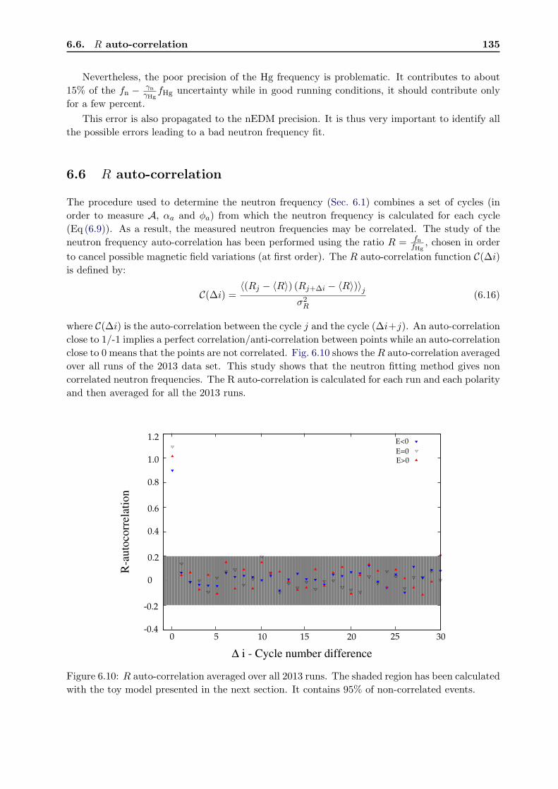
6.6. R auto-correlation 135

Nevertheless, the poor precision of the Hg frequency is problematic. It contributes to about

15% of the fn − γnγHg

fHg uncertainty while in good running conditions, it should contribute only

for a few percent.

This error is also propagated to the nEDM precision. It is thus very important to identify all

the possible errors leading to a bad neutron frequency fit.

6.6 R auto-correlation

The procedure used to determine the neutron frequency (Sec. 6.1) combines a set of cycles (in

order to measure A, αa and φa) from which the neutron frequency is calculated for each cycle

(Eq (6.9)). As a result, the measured neutron frequencies may be correlated. The study of the

neutron frequency auto-correlation has been performed using the ratio R = fnfHg

, chosen in order

to cancel possible magnetic field variations (at first order). The R auto-correlation function C(∆i)

is defined by:

C(∆i) =〈(Rj − 〈R〉) (Rj+∆i − 〈R〉)〉j

σ2R

(6.16)

where C(∆i) is the auto-correlation between the cycle j and the cycle (∆i+j). An auto-correlation

close to 1/-1 implies a perfect correlation/anti-correlation between points while an auto-correlation

close to 0 means that the points are not correlated. Fig. 6.10 shows the R auto-correlation averaged

over all runs of the 2013 data set. This study shows that the neutron fitting method gives non

correlated neutron frequencies. The R auto-correlation is calculated for each run and each polarity

and then averaged for all the 2013 runs.

R-a

uto

corr

elat

ion

Δ i - Cycle number difference

1.2

-0.2

0

0.2

0.4

0.6

0.8

1.0

-0.4302520151050

E>0

E=0

E<0

Figure 6.10: R auto-correlation averaged over all 2013 runs. The shaded region has been calculated

with the toy model presented in the next section. It contains 95% of non-correlated events.

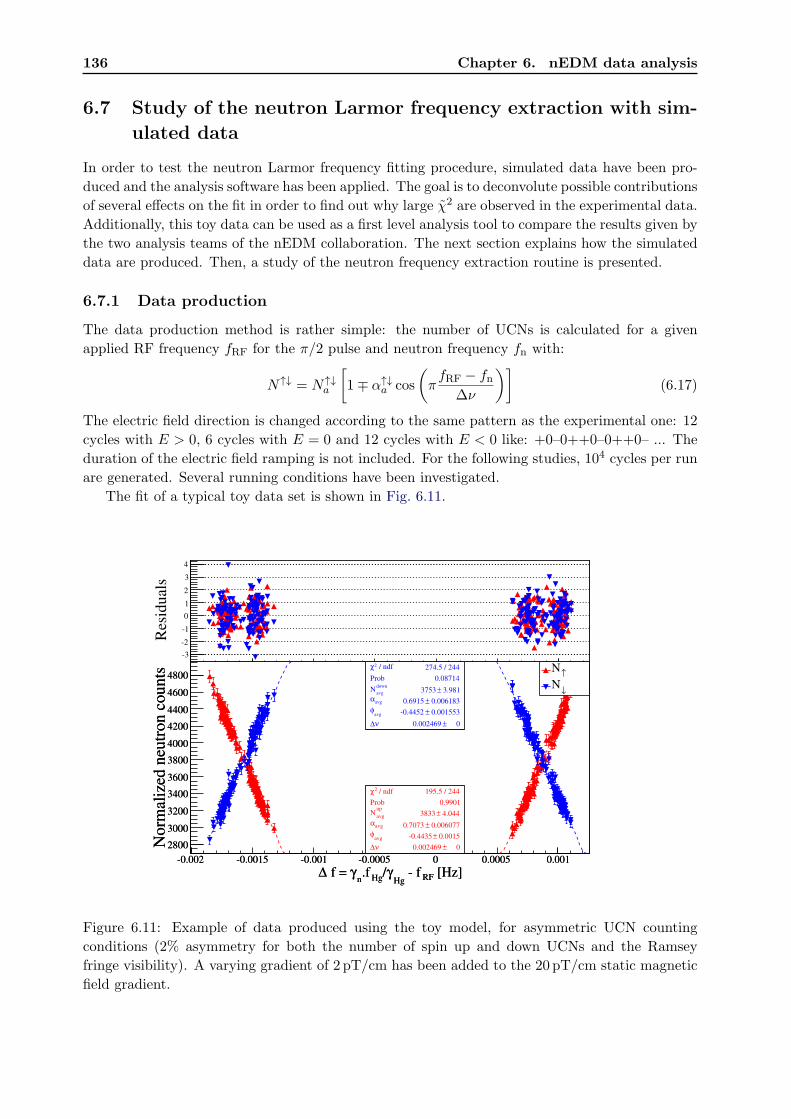
136 Chapter 6. nEDM data analysis

6.7 Study of the neutron Larmor frequency extraction with sim-

ulated data

In order to test the neutron Larmor frequency fitting procedure, simulated data have been pro-

duced and the analysis software has been applied. The goal is to deconvolute possible contributions

of several effects on the fit in order to find out why large χ2 are observed in the experimental data.

Additionally, this toy data can be used as a first level analysis tool to compare the results given by

the two analysis teams of the nEDM collaboration. The next section explains how the simulated

data are produced. Then, a study of the neutron frequency extraction routine is presented.

6.7.1 Data production

The data production method is rather simple: the number of UCNs is calculated for a given

applied RF frequency fRF for the π/2 pulse and neutron frequency fn with:

N↑↓ = N↑↓a

[

1∓ α↑↓a cos

(

πfRF − fn

∆ν

)]

(6.17)

The electric field direction is changed according to the same pattern as the experimental one: 12

cycles with E > 0, 6 cycles with E = 0 and 12 cycles with E < 0 like: +0–0++0–0++0– ... The

duration of the electric field ramping is not included. For the following studies, 104 cycles per run

are generated. Several running conditions have been investigated.

The fit of a typical toy data set is shown in Fig. 6.11.

Res

idual

s

-3

-2

-1

0

1

2

3

4

[Hz]RF - fHg

γ/Hg

.fn

γ f = ∆-0.002 -0.0015 -0.001 -0.0005 0 0.0005 0.001

No

rmal

ized

neu

tro

n c

ou

nts

2800

3000

3200

3400

3600

3800

4000

4200

4400

4600

4800

/ ndf 2χ 195.5 / 244

Prob 0.9901

avg

upN 4.044± 3833

avgα 0.006077± 0.7073

avg

φ 0.0015± -0.4435

ν∆ 0± 0.002469

/ ndf 2χ 195.5 / 244

Prob 0.9901

avg

upN 4.044± 3833

avgα 0.006077± 0.7073

avg

φ 0.0015± -0.4435

ν∆ 0± 0.002469

/ ndf 2χ 274.5 / 244

Prob 0.08714

avg

downN 3.981± 3753

avgα 0.006183± 0.6915

avg

φ 0.001553± -0.4452

ν∆ 0± 0.002469

/ ndf 2χ 274.5 / 244

Prob 0.08714

avg

downN 3.981± 3753

avgα 0.006183± 0.6915

avg

φ 0.001553± -0.4452

ν∆ 0± 0.002469

[Hz]RF - fHg

γ/Hg

.fn

γ f = ∆-0.002 -0.0015 -0.001 -0.0005 0 0.0005 0.001

No

rmal

ized

neu

tro

n c

ou

nts

2800

3000

3200

3400

3600

3800

4000

4200

4400

4600

4800

/ ndf 2χ 195.5 / 244

Prob 0.9901

avg

upN 4.044± 3833

avgα 0.006077± 0.7073

avg

φ 0.0015± -0.4435

ν∆ 0± 0.002469

/ ndf 2χ 195.5 / 244

Prob 0.9901

avg

upN 4.044± 3833

avgα 0.006077± 0.7073

avg

φ 0.0015± -0.4435

ν∆ 0± 0.002469

/ ndf 2χ 274.5 / 244

Prob 0.08714

avg

downN 3.981± 3753

avgα 0.006183± 0.6915

avg

φ 0.001553± -0.4452

ν∆ 0± 0.002469

/ ndf 2χ 274.5 / 244

Prob 0.08714

avg

downN 3.981± 3753

avgα 0.006183± 0.6915

avg

φ 0.001553± -0.4452

ν∆ 0± 0.002469

↑N

↓N

Figure 6.11: Example of data produced using the toy model, for asymmetric UCN counting

conditions (2% asymmetry for both the number of spin up and down UCNs and the Ramsey

fringe visibility). A varying gradient of 2 pT/cm has been added to the 20 pT/cm static magnetic

field gradient.

6.7. Study of the neutron Larmor frequency extraction with simulated data 137

6.7.2 Ideal conditions

The basic running conditions in the toy model follow. The mercury frequency does not change

from cycle to cycle, i.e. the magnetic field does not vary along the run. The Hg T2 time is not

simulated and the Hg frequency statistical error is fixed to 1 µHz. Two values are computed from

the mercury frequency: the π/2 pulse RF frequency fRF and the neutron frequency:

f in = γn

γHgf iHg

f iRF = γn

γHgf i−1Hg ± ∆ν

2 (1± 0.1)(6.18)

The visibility of the fringe αa, the average number of detected neutrons Na, the number of

monitored UCNs... are constant. Statistical fluctuations of the number of detected/monitored

UCNs and the Hg frequency are used.

For such ideal conditions, the reduced χ2 of the neutron frequency fit is 1. The fn − γnγHg

fHg

precision of precision (standard deviation of its distribution) of 13.0±0.2 µHz is in agreement with

the expected value given by Eq (2.15) of 13.2 µHz. Finally, the accuracy of the neutron frequency

extraction is −0.15 ± 0.13 µHz. It is obtained via the mean difference between the simulated

neutron frequencies and the extracted one.

6.7.3 B field fluctuations

In order to reproduce typical magnetic field fluctuations, magnetic field variations from cycle

to cycle have been extracted over a three days run via the Hg frequency (run n 7650). The

distribution of such variations is roughly gaussian, centred on 0 with a standard deviation of

13.5 µHz. In the toy data, the Hg frequency is thus randomly varied according to a gaussian

distribution using these experimental parameters. Typical magnetic field changes are shown in

Fig. 6.12 The simulated magnetic field fluctuation is then applied to the neutron frequency.

Cycle0 100 200 300 400 500 600

[H

z]H

gf

7.829

7.8292

7.8294

7.8296

7.8298

7.83

Figure 6.12: Hg frequency generated along cycles in simulated data.

With B field fluctuations, the reduced χ2 of the neutron frequency fit is 1. The fn − γnγHg

fHg

precision of 13.0 ± 0.2 µHz is in agreement with the expected value of 13.2 µHz. Finally, the

accuracy of the neutron frequency extraction is 0.10± 0.13 µHz. It means that the normalisation

using the Hg frequency is properly performed in the analysis software.

138 Chapter 6. nEDM data analysis

6.7.4 UCN source production decay

The UCN source production decays along time. It has been included in the toy model by means

of a decay time constant of 2.89× 106 s, fitted from the experimental data. Then, non-statistical

fluctuations of the source are also implemented. They amount to approximately 104 counts for a

number of monitored UCNs which is of the order of 8× 105 UCN counts. These fluctuations are

then propagated to the number of detected neutrons.

For such conditions, the reduced χ2 of the neutron frequency fit is 1. The fn− γnγHg

fHg precision

of 15.5 ± 0.2 µHz is in agreement with the expected value of 15.3 µHz. Finally, the accuracy of

the neutron frequency extraction is 0.13± 0.15 µHz. The same results are obtained with both the

asymmetry and the neutron counts fit. It means that the normalisation of the neutron counts

with the monitor properly works and does not affect the fit quality.

6.7.5 Static magnetic field gradient

As seen in Sec. 6.4, a static magnetic field gradient shifts the neutron Larmor frequency with

respect to the mercury one. As a result, the working points location, calculated from the mercury

frequency (as in the data acquisition), are slightly shifted on the Ramsey fringe, with respect to

the resonance frequency. This shift is set using:

∆f∂zBz = ∓ γn2π

(∆h 〈∂zBz〉) (6.19)

where the - and + signs hold for the B0 up and B0 down configurations.

In addition, the fringe visibility is modified by the gradient, according to [110]:

α = α0e−a|〈∂zBz〉| (6.20)

The a parameter is derived from a fit of the 2012 R-curve data giving: a ≃ 3.4×10−4 (pT/cm)−1.

The static magnetic field gradient used for this study is 10 pT/cm. For such conditions, the

reduced χ2 of the neutron frequency fit is 1. The fn − γnγHg

fHg precision of 15.6 ± 0.2 µHz is in

agreement with the expected value of 15.3 µHz. Finally, the accuracy of the neutron frequency

extraction is 0.13± 0.15 µHz.

6.7.6 Daily variation of the magnetic field gradient

Daily variations of the gradient of a few pT/cm peak-to-peak have been observed during

2013 data (see Sec. 6.4). This variation has been implemented in the toy model by means of an

additional time dependent gradient δ 〈∂zBz〉 (t):

δ 〈∂zBz〉 (t) =g02cos

(

2πt

24× 3600

)

(6.21)

Here, a simple ad-hoc cosine function has been taken to model the observed daily gradient varia-

tions but it could be further sophisticated. For g0 = 3pT/cm, the maximum variation of the shift

∆f∂zBz is 20 µHz. As well as for a static gradient, the visibility varies with the field gradient. For

a 3 pT/cm variation and a non-zero static gradient, the visibility change is about 1%. The two

effects are shown in Fig. 6.13 for g0 =10pT/cm. Such a large variation has been used in order to

clearly show the resulting effect on the Ramsey fringe.

In order to meet the experimental conditions, a 2 pT/cm variation of the magnetic field gradient

has been set in addition to a 20 pT/cm static gradient. For such conditions, the accuracy of the

6.7. Study of the neutron Larmor frequency extraction with simulated data 139

1000

2000

3000

4000

5000

6000

7000

8000

9000

10000

11000

-0.004 -0.003 -0.002 -0.001 0 0.001 0.002 0.003 0.004

Nu

mb

er o

f sp

in u

p n

eutr

on

s

fRF-γn/γHgfHg [Hz]

100 pT/cm static gradient+10 pT/cm same α

+10 pT/cm + α effect

Figure 6.13: Illustration of a 10 pT/cm vertical gradient variation effect on the neutron frequency

resonance and the Ramsey pattern visibility. A static magnetic field gradient of 100 pT/cm is also

used. The central fringe is globally shifted towards negative values due to this static magnetic

field gradient.

neutron frequency extraction is 0.15±0.15 µHz. However, the reduced χ2 of the neutron frequency

fit is 1.12. The fn − γnγHg

fHg precision of 16.3± 0.2 µHz is 6.5% larger than the expected value of

15.3 µHz. This behaviour looks like the effect observed in experimental data. This effect is further

investigated in the next section.

6.7.6.1 Effect of a daily gradient variation on the χ2

In order to assess the effect of a gradient variation along a run on the χ2 neutron frequency fit,

toy data have been produced with different input gradient variations g0, with a static gradient of

20 pT/cm. 600 cycles have been generated for each sample. Results are summarized in Fig. 6.14.

As expected, the larger the gradient variation, the larger the χ2. For gradient variations of

2 pT/cm (as observed in experimental data), the reduced χ2 of about 1.15 is consistent with the

average χ2 obtained with the 2013 nEDM runs (see Sec. 6.2 and Sec. 6.3). It does not prove

that the gradient variation is the only source of problems for the neutron frequency fit, but it can

explain the measured χ2.

A possible way to avoid the effect of a slow gradient variation could be to perform the fit on

sub-samples of each run. As a result,the gradient variation is low and the Ramsey fringe visibility

as well as the neutron resonance frequency with respect to the mercury do not change significantly.

This has been tested with the toy model. The pattern used for the electric field polarity changes

is: −0 + 0 − 0+... with 24 cycles for positive or negative polarity and 12 cycles without electric

field.

140 Chapter 6. nEDM data analysis

1

1.05

1.1

1.15

1.2

1.25

1.3

1.35

1.4

1.45

1.5

0 1 2 3 4

Red

uce

d χ

2

Gradient variation [pT/cm]

Figure 6.14: Effect of a cosine daily variation of the magnetic field gradient on the neutron Larmor

frequency fit quality. The point corresponding to the 2 pT/cm gradient variation observed in

experimental data is emphasized.

The averaged resulting χ2 obtained for different number of cycles used to perform the fit and

for different gradient variations is shown in Fig. 6.15. The number of cycles is a multiple of 24. A

large step is visible when going from 24 cycles to 48 cycles. It means that using smaller samples

may help to remove gradient effects on the fit quality.

6.7.7 Relevance of the δ term use

In this part, the relevance of the δ term used in the asymmetry fit function (Eq (6.8)) is studied.

In this study, previous conditions have been included to generate the data. Reasonable running

conditions are used: 〈∂zBz〉 = 20pT/cm, g0 = 2pT/cm. In order to determine the influence of

the δ term on the fit quality, a 2% asymmetry is added between spin up and spin down detection,

both on the number of counts and on the visibility. This is visible in Fig. 6.11.

Whatever the use or not of the δ term, obtained results are the same: the accuracy on the

extracted neutron frequency is of the order of 0.15 µHz. Same results have been obtained using

the normalised neutron counts fitting procedure.

Since no improvement has been observed with the δ term, it has been chosen to perform the

fit without it.

6.7.8 Conclusions on the neutron frequency extraction

Both the experimental study of the neutron Larmor frequency and the use of the toy model have

shown that the analysis code can reliably extract neutron frequencies, even if some checks are

still not present in the current experimental analysis (e.g. the leakage current or the right switch

positioning). The major improvement of the fit quality comes from the development of a new

method for the Hg frequency extraction. This new technique is adapted to low Hg tranverse

relaxation times. It gives improved results, even without taking into account the entire signal.

It has also been shown that the 2 pT/cm gradient variation observed in experimental data

could explain the χ2 of the neutron frequency fit.

6.8. nEDM measurement with 2013 data 141

1.45

1.38

1.32

1.26

1.2

1.15

1.1

1.05

02

46

810

50100

150200

250

1

Reducedχ2

11.051.11.151.21.251.31.351.41.451.5

Cycles per sampleGradient variation [pT/cm]

Figure 6.15: Map of the reduced χ2 as a function of the number of cycles used to perform the fit

and the amplitude of the daily gradient variation. Toy data have been produced using a 50 pT/cm

static gradient.

6.8 nEDM measurement with 2013 data

This 2013 data analysis is based on the work presented in [1, 112]. The neutron Larmor frequency

is extracted using the procedure described in Sec. 6.1, with the asymmetry fit (section 6.1.3).

First, a short overview of nEDM systematic effects is given. Then, the nEDM dmeasn is extracted.

6.8.1 Systematic errors

Using Eq (2.8), the ratio R of the neutron to mercury Larmor frequencies is:

R =fnfHg

=|(µnBn ± dnE)|

|(µHgBHg ± dHgE)| (6.22)

where the + sign corresponds to parallel magnetic and electric fields and the - sign to antiparallel

fields. Here, Bn and BHg correspond to the magnetic fields respectively seen by the neutrons and

the mercury atoms. Assuming that Bn = BHg and considering EDMs to first order, one gets:

R =µnBn

µHgBHg

(

1± dnEµnBn

)

(

1± dHgEµHgBHg

) (6.23)

R ≃ γnγHg

± 2E

hfHg

(

dn −γnγHg

dHg

)

(6.24)

where h is the Planck constant.

Then the nEDM is recovered by means of a linear fit of R versus the electric field E. The raw

dn extracted from Eq (6.24) is given by:

dmeasn = dn −

γnγHg

dmeasHg (6.25)

The measured Hg EDM (which can contain false contributions) propagates to the neutron EDM

itself due to the frequency normalisation.

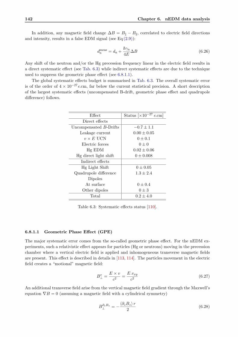
142 Chapter 6. nEDM data analysis

In addition, any magnetic field change ∆B = B‖ − B∦, correlated to electric field directions

and intensity, results in a false EDM signal (see Eq (2.9)):

dmeasn = dn +

~γn4E

∆B (6.26)

Any shift of the neutron and/or the Hg precession frequency linear in the electric field results in

a direct systematic effect (see Tab. 6.3) while indirect systematic effects are due to the technique

used to suppress the geometric phase effect (see 6.8.1.1).

The global systematic effects budget is summarised in Tab. 6.3. The overall systematic error

is of the order of 4 × 10−27e.cm, far below the current statistical precision. A short description

of the largest systematic effects (uncompensated B-drift, geometric phase effect and quadrupole

difference) follows.

Effect Status [×10−27 e.cm]

Direct effects

Uncompensated B-Drifts −0.7± 1.1

Leakage current 0.00± 0.05

v × E UCN 0± 0.1

Electric forces 0± 0

Hg EDM 0.02± 0.06

Hg direct light shift 0± 0.008

Indirect effects

Hg Light Shift 0± 0.05

Quadrupole difference 1.3± 2.4

Dipoles

At surface 0± 0.4

Other dipoles 0± 3

Total 0.2± 4.0

Table 6.3: Systematic effects status [110].

6.8.1.1 Geometric Phase Effect (GPE)

The major systematic error comes from the so-called geometric phase effect. For the nEDM ex-

periments, such a relativistic effect appears for particles (Hg or neutrons) moving in the precession

chamber where a vertical electric field is applied and inhomogeneous transverse magnetic fields

are present. This effect is described in details in [113, 114]. The particles movement in the electric

field creates a “motional” magnetic field:

Bv⊥ =

E × v

c2=

E.vxyc2

(6.27)

An additional transverse field arise from the vertical magnetic field gradient through the Maxwell’s

equation ∇B = 0 (assuming a magnetic field with a cylindrical symmetry)

B∂zBz⊥ = −〈∂zBz〉 r

2(6.28)

6.8. nEDM measurement with 2013 data 143

A ∆ω shift of the particles precession frequency (with respect to ω0 = γB0) is produced. It is

called the Ramsey-Bloch-Siegert shift [115, 116]:

∆ω ≃ (γB⊥)2

2 (ω0 −B⊥/γ)(6.29)

with:

B2⊥ =

(

B〈∂zBz〉⊥ +Bv

⊥)2

(6.30)

= (B〈∂zBz〉⊥ )2 + (Bv

⊥)2 +

〈∂zBz〉 vxyrEc2

(6.31)

where vxy is the particle speed component perpendicular to the electric field, the only speed

contributing in the product #–v × #–

E. Through Eq (6.29) and (6.31), it is visible that the frequency

shift ∆ω has a term linearly proportionnal to E. Because UCNs move slower (adiabatic regime)

than the Hg atoms (non-adiabatic regime), the effect is about 10 to 15 times larger for the mercury

than for neutrons [113] and is transmitted to the false neutron EDM by [114]:

dfalseHg→n =~|γHgγn| 〈∂zBz〉D2

32c2(6.32)

where D is the diameter of the nEDM precession chamber. This effect, estimated in [117], induces

a false neutron EDM of:

dfalseHg→n ≃ 3.8× 10−27 × 〈∂zBz〉 e.cm1 pT/cm

(6.33)

Fortunately, as the false EDM scales linearly with the gradient and also depends on the magnetic

field direction, it is possible to cancel its contribution using the so-called crossing point analysis,

introduced by the RAL-Sussex-ILL collaboration [1]. This method is described and used in 6.8.4.

However, Eq (6.32) only holds for a uniform cylindrical gradient. In the presence of a localised

magnetic field inhomogeneity, for instance a magnetic dipole located close to the precession cham-

ber, the general expression is given by [114]:

dfalseHg→n =~|γHgγn|

2c2〈xBx + yBy〉 (6.34)

Such inhomogeneties have been measured during the mapping of the bottom electrode at the

PTB2. The induced false EDM has been estimated to 0± 3× 10−27 e.cm [118], corresponding to

the “Other dipoles” value in Tab. 6.3.

6.8.1.2 Quadrupole difference

This systematic effect comes from the fact that neutrons and mercury average differently the

magnetic field inside the precession chamber and the use of the crossing point technique. Indeed,

because the neutron Larmor frequency is larger than the UCN wall collision rate (because of the

low UCN speed), UCNs average the modulus of the magnetic field⟨

| #–

B|⟩

. They are able to follow

the magnetic field variation (adiabatic regime). On the contrary, the Hg co-magnetometer, fastly

moving through the precession chamber, probes the modulus of the averaged magnetic field∣

∣

∣〈 #–

B〉∣

∣

∣.

They are not able to follow the magnetic field variation (non adiabatic regime). This difference

propagates to the EDM through the ratio R:

R =fnfHg

=

⟨

| #–

B|⟩

∣

∣

∣〈 #–

B〉∣

∣

∣

≃

⟨√

B2x +B2

y +B2z

⟩

Bz≃ 1 +

⟨

B2T

⟩

2B2z

(6.35)

2Physikalisch-Technischen Bundesanstalt (Berlin)

144 Chapter 6. nEDM data analysis

where⟨

B2T

⟩

is the average of the squared transverse field and Bz ≃ B0 the modulus of the field.

If⟨

B2T

⟩

is different for B↑0 and B↓

0 configurations, the false EDM resulting from the crossing point

analysis is:

dfalsen =~γnγHgD

2

128c2B0∆h

(

⟨

B2T

⟩↓ −⟨

B2T

⟩↑)(6.36)

≃4.55× 10−27 ×

(

⟨

B2T

⟩↓ −⟨

B2T

⟩↑)

e.cm

1 nT2 (6.37)

The magnetic field mapping of the precession chamber during winter shut-down is used to estimate

the squared transverse field difference(

⟨

B2T

⟩↓ −⟨

B2T

⟩↑)

. The 2010 measurement for the nEDM

magnetic field configuration gave:

(

⟨

B2T

⟩↓ −⟨

B2T

⟩↑)= 0.3± 0.5nT2 (6.38)

The resulting false EDM is thus:

dfalsen = (1.3± 2.4)× 10−27 e.cm (6.39)

Using vectorial magnetometers, this quantity could be monitored along EDM runs and used to

correct online this important systematic effect (see Tab. 6.3). A preliminary study of such a

monitoring using vector caesium magnetometers is presented in Chap 7.

6.8.1.3 Uncompensated B-Drifts

When a current (induced by HV charging or discharges) flows in a direction correlated to the

electric field direction, it creates a small magnetic field which may magnetise the innermost mag-

netic shield layer. This magnetisation induces a dipole like field, correlated to the electric field

direction. The corresponding gradient change is differently seen by neutrons and Hg because of

their different centres of mass. The gradient difference ∆ 〈∂zBz〉 between the two electric field

polarities gives a B field difference ∆ 〈∂zBz〉∆h, not compensated by the Hg co-magnetometer.

Such an effect has been estimated during dedicated measurements in 2012, giving the induced

false EDM 3:

dfalsen = (−0.7± 1.1)× 10−27 e.cm (6.40)

It has to be noticed that measurements have not been carried out as in nEDM measurements, but

during a shorter time with a constant electric field. As a result, the number of electric discharges

is likely different in this measurement compared to EDM data taking conditions.

6.8.2 Raw nEDM extraction

Back to Eq (6.24), the nEDM recovery can be performed through the slope of a linear fit of R

versus the applied High Voltage (HV), such as R = R0 + s.HV . The slope s is equal to:

s =2(

dn − γnγHg

dHg

)

dElechfHg(6.41)

where dElec = 12 cm is the distance between the two electrodes. An example of such a fit is shown

in Fig. 6.16.

3A recent re-analysis of data from 2010 to 2013 data estimates the false EDM coming from the uncompensated

B-drift to (−0.05± 0.43)× 10−27e.cm.

6.8. nEDM measurement with 2013 data 145

The current limit on the mercury EDM dHg = (0.49± 1.29± 0.79) × 10−29 e.cm [55] induces

a negligible systematic effect on the neutron EDM:

dfalseHg→n = (1.9± 5.0± 3.1)× 10−29 e.cm

The ratio R is calculated using the neutron precession frequency extracted for each cycle and

the corresponding Hg frequency estimated by the s/n method (see 6.3.1). The error on the Hg

frequency takes into account the factor 6 coming from the use of the Hg signal bandpass filters

[108].

High Voltage [kV]

-100 -50 0 50 100

R

3.842426

3.8424262

3.8424264

3.8424266

3.8424268

3.842427 / ndf 2χ 0.6871 / 1

Prob 0.4072

p0 1.173e-07± 3.842

p1 1.143e-09± -2.711e-09

/ ndf 2χ 0.6871 / 1

Prob 0.4072

p0 1.173e-07± 3.842

p1 1.143e-09± -2.711e-09

Graph

Figure 6.16: nEDM extraction via the fit of R versus High Voltage.

For more than half of 2013 EDM runs (7 runs over 12), the reduced χ2 of the fit is above

4.5. Such χ2 can not be statistically explained. The reasons for which the relation R = f(E) is

not fully linear is not understood yet. Electric discharges are possible candidates to explain such

non linearity. The study of the leakage current between the shutter opening and closing has to

be performed in order to find possible sparks which could influence the magnetic field during the

precession. Nevertheless, the data analysis has been continued in order to determine the statistical

precision reached with the 2013 data.

A summary of 2013 EDM runs used in this analysis as well as their running conditions are

presented in the appendixC. The expected nEDM statistical error calculated from Eq (2.17) does

not agree with the measured precision. However, if the bad χ2 of the neutron Larmor frequency

fit and the Hg frequency error (which propagates to the ratio R) are taken into account, the

measured dn precision becomes consistent with expectations for 5 runs over 13. The remaining 8

runs have a measured precision 11% larger than the expected one in average. Study is ongoing.

Summing all the runs, the total expected dn sensitivity is 0.80× 10−25 e.cm (by rescaling with

the Hg frequency statistical error and the neutron Larmor frequency fit reduced χ2 as previously).

The total measured nEDM sensitivity has been extracted as follows. The measured nEDM have

been plotted as a function of Ra − 1 (see Eq (6.49)) for B0 up and B0 down configurations and

have been fitted by a constant, as shown in Fig. 6.17.

146 Chapter 6. nEDM data analysis

-1 [ppm]aR-6 -4 -2 0 2 4 6

e.cm

]-2

510

×[n

d

-25

-20

-15

-10

-5

0

5

10

/ ndf 2χ 6.535 / 6

p0 1.122±1.802

/ ndf 2χ 6.535 / 6

p0 1.122±1.802

/ ndf 2χ 9.851 / 5

p0 1.397±-2.833

/ ndf 2χ 9.851 / 5

p0 1.397±-2.833

B down

B up

Figure 6.17: Constant fits of the B0 up and the B0 down nEDM data. B0 up correspond to the

up red triangles and B0 down to the down blue triangles.

Combining the results for each magnetic field direction, one gets:

d↑n = (−2.8± 1.4)× 10−25e.cm χ2 = 1.97 (6.42)

d↓n = (+1.8± 0.9)× 10−25e.cm χ2 = 1.08 (6.43)

it results in the nEDM measurement of 2013 data without the GPE correction:

dn = (−0.50± 0.83)× 10−25e.cm (6.44)

The measured statistical sensitivity is about 4% larger than the expected one. But this measure-

ment does not account for the geometric phase effect. The GPE correction is done later using the

so-called crossing-point analysis.

6.8.3 Correction of the Earth’s rotation frequency shift

Because the neutron spin precession is observed in the Earth frame and not in a fixed frame, the

Earth rotation adds up or subtracts from the Larmor precession frequency, according to the B0

direction. Its contribution to the ratio R amounts to [119]:

δEarthR = ± γnγHg

ΩT sinλ

B0

(

1

|γHg|+

1

|γn|

)

(6.45)

where ΩT = 11.6 µHz is the sideral angular rotation frequency of the Earth and λ = 47.517 is

the PSI latitude. The + and - signs respectively hold for the B0 up and B0 down configurations.

The effect on R is thus:

R =γnγHg

+ δEarthR =γnγHg

± 5.3ppm (6.46)

This effect has been taken into account to perform the crossing point analysis, presented in the

next part.

6.8. nEDM measurement with 2013 data 147

6.8.4 Suppression of the geometric phase effect

The false EDM coming from the geometric phase of the Hg depends on the vertical magnetic field

gradient as well as the R ratio. This common property is used for the crossing point analysis.

One writes:

R ≃ γnγHg

(

1∓ ∆h 〈∂zBz〉B0

)

(6.47)

Where the - and + signs correspond respectively to B0 up and B0 down configurations. The

vertical gradient can be expressed as a function of R

〈∂zBz〉 = ∓(

RγHg

γn− 1

)

B0

∆h(6.48)

= ∓ (Ra − 1)B0

∆hwith Ra = R

γHg

γn(6.49)

As a result, Eq (6.32) gives:

dfalseHg→n = ∓h|γn|fHgD2

32c2∆h(Ra − 1) (6.50)

Thus, there is a linear dependence between the false EDM dfalseHg→n and Ra − 1.The curve corre-

sponding to the B0 up configurations and the curve associated to the B0 down configurations

have opposite slopes. They cross at the point where Ra − 1 = 0. For such a point, the false

EDM induced by the GPE is null. This is the so-called crossing point technique pioneered by the

RAL-Sussex-ILL collaboration [1].

Using the value ∆h = 0.235±0.005 cm extracted during the 2012 R-curve measurements [109],

the expected slope sGP of Eq (6.50) can be calculated:

sGP = ∓ (6.67± 0.14)× 10−20e.cm/ppm (6.51)

The error bar of the slope comes from the uncertainty of ∆h.

The crossing point analysis has been performed over the 2013 nEDM runs as shown in Fig. 6.18.

For both field directions, the slope is consistent with the expected one:

s↑GP = − (3.7± 3.6)× 10−20e.cm/ppm χ2 = 2.20 (6.52)

s↓GP = +(7.8± 5.0)× 10−20e.cm/ppm χ2 = 0.82 (6.53)

Two runs belonging to the B0 up configuration are off the expected curve (Ra − 1 ≃ −5 ppm

and Ra − 1 ≃ −7 ppm), particularly one at more than 3σ. This is likely related to the problem

observed in 6.8.2, since these two runs belong to the data set with a non-statistical behaviour for

the fit which determines dmeasn . Investigations are still ongoing.

As a result, the precision of the slopes is poor and the coordinates of the crossing point are

not precise: Ra − 1 = −5.9± 3.8 ppm and dn = (−2.3± 3.4)× 10−25 e.cm.

148 Chapter 6. nEDM data analysis

-1aR-6 -4 -2 0 2 4 6

e.cm

]-2

510

×[n

d

-25

-20

-15

-10

-5

0

5

10/ ndf 2χ 4.112 / 5

p0 1.173±2.33

p1 0.5036±0.7836

/ ndf 2χ 4.112 / 5

p0 1.173±2.33

p1 0.5036±0.7836

/ ndf 2χ 8.814 / 4

p0 2.145±-4.491

p1 0.3643±-0.371

/ ndf 2χ 8.814 / 4

p0 2.145±-4.491

p1 0.3643±-0.371

B up

B down

[ppm]

Figure 6.18: Crossing point analysis of 2013 nEDM data. The B0 up configurations correspond

to the up red triangles and the B0 down configurations to the down blue triangles.

6.9 Conclusion

From both the experimental analysis and the toy model results, the reliability of the neutron

Larmor frequency extraction has been studied.

Using simulated data, the accuracy of the fit has been estimated to be about 0.15 µHz. The

statistical precision is in agreement with the expected one for both simulated and experimental

data.

With simulated data, the reduced χ2 is equal to 1 using usual running conditions. For experi-

mental data, the average reduced χ2 of the neutron Larmor frequency fit is larger (χ2 ≃ 1.15). A

possible explanation supported by simulations has been pointed out. A small and slow magnetic

field gradient variation (with a daily period for instance) deteriorates the fit quality. In the toy

model, a daily sinusoidal variation of the vertical magnetic field gradient with a 2 pT/cm ampli-

tude produces a χ2 ≃ 1.14, consistent with observations. A possible way to suppress this effect is

to use smaller data samples, for both the neutron Larmor frequency fit and the nEDM extraction.

However, it has recently been shown that this magnetic field gradient is correlated to temperature

changes [111]. Therefore, a better thermal insulation and stabilisation of the thermohouse would

be more efficient.

During the last stage of the nEDM analysis, it has been shown that the Hg frequency precision

is critical and may significantly degrade the nEDM precision. The collaboration is actively working

to find out the source of the low Hg transverse relaxation time, which is the cause of the low Hg

frequency precision. A new method has been developped, the s/n Hg frequency fitting method. It

is more suited to the bad Hg running conditions than the usual two windows method. However,

a problem with this new technique is not excluded, since it does not average the magnetic field

during the full neutron precession.

Finally, the last part of the 2013 nEDM analysis pointed out a problem for the dn recovery

via the linear fit of R versus E. For more than 50% of EDM runs, the reduced χ2 of this fit

lies above 4.5, meaning that an additionnal non-expected effect correlated to the electric field

6.9. Conclusion 149

is present in the data. Further investigations are required. In spite of this important problem,

the 2013 data was analysed. The outcoming result is a preliminary estimation of the nEDM:

dn = (−2.3± 3.4)× 10−25 e.cm.

Vertical magnetic field gradient variations may degrade the neutron Larmor frequency fit.

They have been measured with the scalar caesium magnetometers array. The next chapter is

dedicated to the test and the improvement of methods used to extract magnetic field observables

from caesium data, relevant for the control of systematic effects.

Chapter 7

Study of magnetic observables

estimators

Contents

7.1 Harmonic polynomials series expansion . . . . . . . . . . . . . . . . . . . . 153

7.2 Toy model principle . . . . . . . . . . . . . . . . . . . . . . . . . . . . . . . . 155

7.3 Methods used to determine the vertical gradient . . . . . . . . . . . . . . 155

7.3.1 Top-Bottom averaging . . . . . . . . . . . . . . . . . . . . . . . . . . . . . . . 155

7.3.2 Pairs . . . . . . . . . . . . . . . . . . . . . . . . . . . . . . . . . . . . . . . . . 155

7.3.3 Harmonic Taylor fit of Bz . . . . . . . . . . . . . . . . . . . . . . . . . . . . . 156

7.4 R-curve gradients reproducibility with 2013 maps . . . . . . . . . . . . . . 156

7.5 Comparison of the three methods . . . . . . . . . . . . . . . . . . . . . . . 157

7.5.1 Comparison in R-curve configurations . . . . . . . . . . . . . . . . . . . . . . 157

7.5.2 Transverse field components effect on the gradient estimate . . . . . . . . . . 159

7.5.3 Harmonic Taylor fitting method improvement . . . . . . . . . . . . . . . . . . 160

7.6 Test of a 3D harmonic fit . . . . . . . . . . . . . . . . . . . . . . . . . . . . . 161

7.6.1 Improvement of the 3D harmonic fit . . . . . . . . . . . . . . . . . . . . . . . 162

7.7 Conclusions . . . . . . . . . . . . . . . . . . . . . . . . . . . . . . . . . . . . . 163

7.1. Harmonic polynomials series expansion 153

As seen previously, the Hg co-magnetometer and ultra cold neutrons do not average the same

magnetic field during the free precession time. Combined to a non-zero vertical gradient, this

gives rise to several systematic effects (gravitational shift, geometric phase effect). In order to

determine these systematics, an array of optically pumped scalar caesium magnetometers (CsM)

is used to measure the vertical gradient inside the precession chamber (see 3.4.3.2). The vertical

gradient has also been used in the 2012 R-curve measurements to determine the centre of mass

difference ∆h and to estimate the ratio γn/γHg.

In this section, the different ways to estimate the vertical gradient through the CsM data are

studied. A prospective study for the n2EDM phase is also presented, testing the efficiency of

3D CsM to extract information about the transverse fields, involved in the so-called quadrupole

difference systematic effect.

7.1 Harmonic polynomials series expansion

In order to parametrise the magnetic field inside the precession chamber, a new set of Cartesian

harmonics has been developed [120]. This set of harmonic polynomials can be used to expand the

magnetic scalar potential Ψ, solution of the Laplace’s equation in a magnetisation and current-free

region:

∇2Ψ( #–r ) = 0 (7.1)

such as:

Ψ( #–r ) =∞∑

n=0

HnQn(#–r ) (7.2)

The magnetic induction#–

B = −∇Ψ is then given by:

#–

B( #–r ) =

Bx(#–r )

By(#–r )

Bz(#–r )

=∞∑

n=1

Hn

Pxn(#–r )

Pyn(#–r )

Pzn(#–r )

(7.3)

where Pin(#–r ) = −∂iQn(

#–r ) i = x, y, z. The harmonic polynomials#–

P in(#–r ) are listed in Tab. 7.1

up to the order 15.

Once the spectrum Hn is known, i.e. once the Hn coefficients are known up to a given

order, it is then possible to perform the harmonic synthesis of the magnetic field (Eq (7.3)) and

to determine the field everywhere in a mapped volume VCh.

In the case of the nEDM experiment, the harmonic spectra of the main coils have been ex-

tracted by fitting fluxgate 3D magnetic field maps, performed with a mapper designed and built at

LPC Caen during winter 2013 [121, 122]. The mapped volume is a bit larger than the precession

chamber and includes the caesium magnetometers arrays as shown in Fig. 7.1. This has been

obtained using 5 z planes (−160,−80, 0, 80, 160 mm), 2 cm radius steps up to 35 cm with 10

azimutal steps. The best reduced χ2 has been found for an expansion of the field up to the fourth

degree, equivalent to the harmonic order 35.

One has now the ability to produce a magnetic field at every position in the mapped volume

and for instance test methods for extracting the averaged vertical gradient over the precession

chamber volume. The presentation of this toy model is the topic of the following section.

154 Chapter 7. Study of magnetic observables estimators

Hn Pxn(#–r ) Pyn(

#–r ) Pzn(#–r )

H1 1 0 0

H2 0 1 0

H3 0 0 1

H4 x 0 −z

H5 y x 0

H6 0 y −z

H7 z 0 x

H8 0 z y

H9 x2 − z2 0 −2xz

H10 2xy x2 − z2 −2yz

H11 y2 − z2 2xy −2xz

H12 0 y2 − z2 −2yz

H13 2xz 0 x2 − z2

H14 yz xz xy

H15 0 2yz y2 − z2

......

......

Table 7.1: Harmonic polynomials series expansion for the three components of the magnetic field

up to order 15. Higher order polynomials are tabulated in [120].

super-bottom

z

Figure 7.1: The blue rectangle corresponds to the mapped volume VCh during the 2013 mapping

campaign.

7.2. Toy model principle 155

7.2 Toy model principle

As said previously, from the 3D fluxgate maps, one extracts the harmonic spectrum of different

coils used for the magnetic field homogenisation or for the spin guiding along tubes in the appara-

tus. From these harmonic spectra, the modulus of the magnetic field at caesium magnetometers

positions is produced for a given coil currents configuration. Then, the vertical gradient created

for this field configuration is estimated using the different existing methods (see Sec. 7.3).

Because the total harmonic spectrum is given as an input, the averaged vertical gradient over

the chamber volume coming from the map is calculated:

〈∂zBz〉inputVCh=

1

VCh

∫

VCh

∂zBzdV (7.4)

〈∂zBz〉inputVCh= − (H4 +H6)−

(

z22 − z21) (H13 +H15)

HCh

+ (H16 +H18 +H20)

[

(

z32 − z31)

HCh− 3R2

Ch

4

]

+ (H31 +H33 +H35)

[

(

z42 − z41)

HCh− 3

2

(

z22 − z21)

R2Ch

HCh

]

(7.5)

where z2 = 80mm and z1 = −40mm are respectively the top and bottom electrodes locations,

HCh = 120mm is the height of the precession chamber and RCh = 235mm its radius.

Finally, the gradient estimated by each method 〈∂zBz〉meth is compared to the input average

gradient through the difference ∆ 〈∂zBz〉 = 〈∂zBz〉input − 〈∂zBz〉meth in order to find the best

estimation, giving at the same time the accuracy of each method for a given field configuration.

7.3 Methods used to determine the vertical gradient

Three methods have been used to extract the average vertical gradient 〈∂zBz〉. Two of them are

based on the difference of magnetic field modulus between two z planes. The other one uses a

parametrisation of the field like the one presented previously in Sec. 7.1.

7.3.1 Top-Bottom averaging

The top-bottom averaging method consists in averaging the field seen by the top layer of caesium

magnetometers and by the bottom one and then in extracting the gradient by subtracting the two

values:

〈∂zBz〉tb =〈B〉top − 〈B〉bottom

d(7.6)

with d = 251 mm the vertical distance between the 2 CsM layers (see Fig. 7.1).

This method is simple and does not take into account magnetometers location in each layer.

Another method, which cares about Cs magnetometers positions is briefly described thereafter.

7.3.2 Pairs

The pairs method is basically the same method as the previous one except that only magnetometers

having the same x and y position and occupying two different z layers can be coupled together in

order to extract the vertical gradient.

〈∂zBz〉Pairs =⟨

Btop −Bbottom

d

⟩

Pairs

(7.7)

156 Chapter 7. Study of magnetic observables estimators

Once again, the position of magnetometers is not fully taken into account. Besides, the full

available information is not used: magnetometers which are not paired are useless for this analysis.

7.3.3 Harmonic Taylor fit of Bz

Another method has been initially used by G. Pignol [123] to extract the vertical gradient during

R-curve measurements in September 2012. This method uses the fact that during nEDM data

taking, the magnetic field is mostly vertical in the usual coordinates frame (along the electric

field direction). Using the assumption that transverse components of the field are very small

compared to the vertical component, || #–

B|| ≃ Bz. This means that the modulus seen by caesium

magnetometers can be considered to be approximately the vertical component of the field.

Starting from that point, it is possible to parametrise the measured field by a Taylor fit series

expansion:

|| #–

B|| ≃ Bz = B0z + gxx+ gyy + gzz + gxx(x2 − z2) + gyy(y

2 − z2) + gxyxy + gxzxz + gyzyz (7.8)

This expansion uses the same spatial dependence as the harmonic polynomials series expansion

presented in Sec. 7.1. The correspondence between coefficients in Eq (7.8) and those shown in

Tab. 7.1 is presented in Tab. 7.2.

B0z gx gy gz gxx gyy gxy gxz gyzH3 H7 H8 −H4 −H6 H13 H15 H14 −2(H9 +H11) −2(H10 +H12)

Table 7.2: Correspondence between harmonics coefficients and Taylor coefficients up to order 15

(polynomials of degree 2).

The position of each magnetometer being known, one can then fit the field seen by CsM

using Eq (7.8). Indeed, one has at most 16 operating magnetometers, which is enough degrees

of freedom to extract the 9 parameters of the harmonic Taylor series (7.8). Using some of those

fitted parameters, it is then possible to get back to the vertical gradient:

〈∂zBz〉fitVCh= gz −

(

z22 − z21) (gxx + gyy)

HCh(7.9)

Error bars on the estimated gradient coming from the Taylor fit are obtained by means of the

Jackknife estimator [124].

7.4 R-curve gradients reproducibility with 2013 maps

The goal of the toy model is to extract the error done during the vertical gradient estimation.

Before applying this tool, it has to be shown that the reconstructed magnetic field from 2013 maps

reproduces well the vertical gradient measured in real data. For such a purpose, a comparison has

been performed between toy data and experimental 2012 R-curve data.

The different R-curve coils configurations have been reconstructed (with several B0 maps).

Then, the estimated Taylor fit gradient from the map 〈∂zBz〉map is compared with the gradient

estimated from R-curve data 〈∂zBz〉exp. Fig. 7.2 shows the difference between the two estimated

gradients as a function of the R-curve run number.

7.5. Comparison of the three methods 157

-30

-20

-10

0

10

20

30

40

50

60

70

6020 6030 6040 6050 6060

⟨∂z

Bz⟩

exp-⟨

∂z

Bz⟩

map

[p

T/c

m]

Run number

B0 upB0 down

Figure 7.2: Difference between the estimated gradients from R-curve data and the reconstructed

map as a function of the R-curve run number.

The mean difference between the extracted gradients, estimated through its RMS value,

amounts to 9.9 pT/cm for B0 up and to 16.8 pT/cm for B0 down.

The largest gaps are observed for runs with larger currents in TTC and BTC (coils creating

the vertical gradient), i.e. for larger vertical gradients (∼150 pT/cm). It could mean that there

is a problem with the reproduction of the field created by TTC or BTC. This is supported by

the fact that residuals coming from the fit of the input BTC 2013 map have an unusual spread of

about 3 nT on Bz, indicating a bad fit result [125]. This procedure has to be tried again with the

new 2014 fluxgates maps in order to make sure that there is no problem with the map of this coil.

The conclusion of this check is that the online and offline gradient estimations give results

consistent at the 15 pT/cm level. The difference can be partly explained by a gradient repro-

ducibility of 6 pT/cm for both B0 up and and down maps. Another reason could be that, on

one hand, the fit is performed on perfect CsM data (reconstructed maps) and on the other hand,

it is performed on real CsM data, in experimental conditions (CsM offsets due to cross-talk...).

Finally, the reconstruction of the field using the 2013 maps is good enough to test the different

gradient estimations.

7.5 Comparison of the three methods

7.5.1 Comparison in R-curve configurations

For this comparison, only two layers of CsM are used (as used for the 2012 R-curve and nEDM

data taking) even if two super-bottom CsM are available. The difference between the vertical

gradient from each method and the reconstructed map (used as input for the toy model) is shown

in Fig. 7.3 for different gradients / currents in TTC and BTC, and for B0 up field configuration.

158 Chapter 7. Study of magnetic observables estimators

up 0B

[pT/cm]zBz∂-200 -100 0 100 200

[pT

/cm

]z

Bz∂

Δ

-40

-30

-20

-10

0

10

20

30

[mA]BTC

=-iTTC

i-2 -1.5 -1 -0.5 0 0.5 1 1.5 2

Top-Bottom

Pairs

Taylor fit

- R-curve - With rem. field subtraction

Figure 7.3: Difference between the estimated gradients and the reconstructed map gradient as a

function of the input vertical gradient.

The difference between the input gradient and the estimated one can be expressed as a function

of the input gradient:

∆ 〈∂zBz〉 = a 〈∂zBz〉input + b (7.10)

Fitted parameters values for each method are summarised in Tab. 7.3 for B↑0 and B↓

0 .

MethodB↑

0 B↓0

a [%] b [pT/cm] a [%] b [pT/cm]

Top-Bottom -9.16(24) -1.58(33) -9.10(36) -0.19(52)

Pairs -11.22(26) -1.14(36) -11.15(38) 7.05(56)

R-curve Taylor fit -4.50(76) -1.56(56) -4.45(84) -1.5(10)

Table 7.3: Fitted parameters obtained from Eq (7.10) for each method.

The harmonic Taylor fit is the most accurate method, with the smaller slope. The gap between

the input and the fitted values is lower than 7 pT/cm for currents used for the R-curve analysis,

i.e. for currents in TTC-BTC between -1 and 1 mA. Besides, the non accuracy of the Taylor fit

is consistent with 0 within error bars (see Fig. 7.3), which validates the Jackknife tool to estimate

the statistical error on the gradient.

The map reconstruction has been done for all 2012 R-curve configurations in order to get an

estimation of the gradient uncertainty coming from the harmonic Taylor fit in the framework of

the γn/γHg measurement. Results are shown in Fig. 7.4. The RMS values for B0 up and B0 down

configurations are respectively 3.7 pT/cm and 4.7 pT/cm. For the other methods, the difference

is larger, particularly for the pairs method. Thus, even if the precision of the averaging methods

is better than the harmonic Taylor fit, their accuracy is lower.

7.5. Comparison of the three methods 159

-15

-10

-5

0

5

10

15

20

25

-1 -0.5 0 0.5 1

∆⟨∂

z B

z⟩ [

pT

/cm

]

Current in TTC [mA]

B0 upB0 down

Figure 7.4: Difference between the input gradient and the estimated gradient for all 2012 R-curve

current configurations, using the harmonic Taylor fit.

It has to be noticed that the super-bottom CsM (z = −175mm) use decreases the accuracy of

the Taylor fit by a factor 2, down to the same level as averaging methods. This is thought to be

due to a larger fit sensitivity to high order field harmonics because of the large super-bottom CsM

z position. It brings the idea to study the effect of the CsM positioning around the precession

chamber on fit results. This study could help to improve the harmonic Taylor fit method and

could be important in order to choose the CsM positions for further data taking with oILL and

n2EDM.

7.5.2 Transverse field components effect on the gradient estimate

Because the harmonic Taylor fit is based on the assumption that || #–

B|| ≃ Bz, the effect of a large

transverse field component on the gradient extraction has been studied. The H1B coil brings a

main contribution along By. The difference of average gradients ∆ 〈∂zBz〉 as a function of the

By component created by the H1B coil up to order 15 is shown in Fig. 7.5. The field has only

been produced until harmonic 15 in order to make sure that all Bz terms can be fitted during the

harmonic Taylor fit.

The usual largest transverse fields one expects during nEDM data taking are at the 10 nT

level. The studied range is larger in order to see limits of each method in terms of accuracy. The

harmonic Taylor fit gives again the best results, below the 0.5 pT/cm level error, followed by the

averaging methods which are at worst 5 pT/cm accurate for rather large transverse fields of 10

nT (the -11 pT/cm offset for the pairs method is obviously not due to the transverse field itself).

The conclusion of this study is that low order transverse fields are not a problem for the harmonic

Taylor fitting method, but could be problematic for the top-bottom averaging method.

160 Chapter 7. Study of magnetic observables estimators

up - Transverse field effect - R-curve - With rem. field subtraction0B

[nT]yB-60 -40 -20 0 20 40 60

[pT

/cm

]z

Bz∂

Δ

-40

-30

-20

-10

0

10

20

Top-Bottom

Pairs

SVD

Figure 7.5: Difference between the estimated gradients and the reconstructed map gradient as a

function of the By field component strength. The field is only reconstructed using the B0 coil (up

direction) and the H1B coil.

7.5.3 Harmonic Taylor fitting method improvement

It has been shown in the previous section that the transverse field effect on the gradient estimate

by means of the harmonic Taylor fit is lower than the 0.5 pT/cm level for usual transverse fields.

The remain of the harmonic fit non-accuracy is mainly due to the field contribution of harmonics

higher than 15. Indeed, higher harmonics are not fitted because of the limited number of CsM (12

here). This effect is visible in Fig. 7.6 where is shown the difference of average gradients ∆ 〈∂zBz〉as a function of the last harmonic used to produce the magnetic field. To further emphasise the

effect, a B0 up R-curve configuration with 1/-1 mA currents in TTC/BTC coils is used as an

example.

The first observation is that the Taylor fit is accurate up to the order 15, the last fitted

harmonics. Then, for harmonics 16, 20 and 31, a clear step in the error is visible. This is

explainable looking at the terms difference between (7.5) and (7.9). In the Taylor fit, 3 harmonic

coefficients for 3rd (H16,H18,H20) and 4th (H31,H33,H36) degrees polynomials, contributing to the

mean gradient, are not taken into account. The consequence of that is first to decrease the fit

accuracy, but also to decrease its precision, for instance as visible starting from harmonics 20 with

error bars increased from 2 pT/cm to more than 5 pT/cm. Therefore, a possible improvement

for next steps of the nEDM experiment in the vertical gradient control could be to use more CsM

located on different z layers in order to be able to fit those 6 additional harmonics which have a

non negligible contribution to the average vertical gradient.

To test this possibility, it was first assumed that all CsM located around the precession cham-

ber work but the super-bottom, i.e. 14 magnetometers in total. The additional fitted parameters

are (H16,H18,H20) and H31, increasing the number of fit parameters up to 13. This time, the dif-

ference between the reconstructed map gradient and the fitted gradient does not exceed 3.6 pT/cm

(〈∂zBz〉input ∼ 120 pT/cm). In average, this difference has been decreased from 4.7 and 3.7 pT/cm

7.6. Test of a 3D harmonic fit 161

Harmonic order0 5 10 15 20 25 30 35

[pT

/cm

]z

Bz∂

Δ

-15

-10

-5

0

5

up - R-curve - With rem. field subtraction0

B

Top - BottomPairsTaylor fit

Figure 7.6: Difference between the estimated gradients and the reconstructed map gradient as a

function of the last harmonics used to produce ~B.

for respectively B0 down and B0 up configurations down to 1.9 and 1.3 pT/cm using the fit with

additional harmonics. It shows that the harmonic Taylor fit can be improved by carefully selecting

the harmonics to be fitted.

7.6 Test of a 3D harmonic fit

The vertical gradient is not the only magnetic field observable which induces a false EDM. The

squared transverse field to the main field direction⟨

B2⊥⟩

is also the source of a systematic error

during the so-called crossing point analysis (see 6.8.1.2). The false EDM arising from⟨

B2⊥⟩

is

given by:

dfalse =~γnγHgD

2

128c2B0∆h

(

⟨

B2⊥⟩↓ −

⟨

B2⊥⟩↑)

(7.11)

For the moment, scalar CsM which are used can not provide enough information to recover

this transverse component by means of the harmonic Taylor fit. The related systematic error is

currently estimated through the magnetic field maps which are measured each winter shut-down.

Current estimates of⟨

B2⊥⟩

give values at the 1-2 nT2 level with precisions of about 0.5 nT2.

A possible way to get online the systematic effect in the near future could be to use 3D

caesium vector magnetometers [126] and perform a full 3D harmonic fit on the field created from a

reconstructed map [127]. The aim of such a method is to determine⟨

B2⊥⟩

as accurately as possible

in order to correct precisely the corresponding systematic effect and keep a good determination

of the vertical gradient.

The goal of the following study is to use the same toy model as previously and replace scalar

CsM by 3D vector CsM in order to get an idea of the reachable accuracy on⟨

B2⊥⟩

using 3D

magnetometers. This time, the fit is performed using the R-curve CsM configuration with two

additional CsM on the top plate in order to have 16 CsM values (to be able to fit 15 parameters).

The fit is performed now on the three field components and not only on the field modulus (|| #–

B|| ≃Bz). From the 15 fitted first harmonics, the average field over the precession chamber volume 〈 #–

B〉

162 Chapter 7. Study of magnetic observables estimators

is recovered by Monte-Carlo. Then, the average transverse field is recovered by averaging:

B⊥(#–r )2 = B( #–r )2 −

(

#–

B( #–r ).〈 #–

B〉||〈 #–

B〉||

)2

(7.12)

Then, the average value of B⊥(#–r )2 over the chamber volume obtained with the harmonic fit

is compared to the value obtained from the reconstructed map itself 〈B2⊥〉map. In average, the

reachable accuracy given by the fit is about 0.2 nT2.

At the same time, the average gradient over the chamber volume is recovered through the

15 first harmonics. Again, because (H16,H18,H20,H31) are not fitted, the accuracy of the fit is

limited, here to about 20 pT/cm.

7.6.1 Improvement of the 3D harmonic fit

In order to reach a better accuracy on⟨

B2⊥⟩

, it is possible to use the same method as for the

vertical gradient, i.e. by identifying the harmonics at larger orders contributing to the observable

of interest. An example of such contributions is shown in Fig. 7.7 for a B0 up configuration with

1/-1 mA currents in TTC/BTC (which showed the largest⟨

B2⊥⟩

difference of about 0.5 nT2).

0

0.1

0.2

0.3

0.4

0.5

0.6

0 5 10 15 20 25 30 35

∆⟨B

⊥2 ⟩

[n

T2]

Harmonic order

B0 up

Figure 7.7: Difference between the estimated⟨

B2⊥⟩

from the 3D harmonic Taylor fit and from the

reconstructed map as a function of the last harmonics used to produce ~B.

From this study, harmonics H16, H20 and H31 show a rather large influence on the⟨

B2⊥⟩

determination with the 3D harmonic fit for B0 up configurations (H18 is also important for B0

down configurations). As a result, it shows that these harmonics, already important for the

gradient estimation, have to be fitted in order to estimate the transverse field properly. In order

to fit these additional parameters, one needs more 3D magnetometers around the precession

chamber.

Four virtual additional CsM have been placed around the precession chamber at cardinal

positions, at z = 0, and at r = 300mm. With these magnetometers, one ends up with a total

7.7. Conclusions 163

of 20 vector magnetometers used to fit 19 parameters. The difference of⟨

B2⊥⟩

between the 3D

harmonic fit and the reconstructed map is shown in Fig. 7.8 for each field configuration used

during R-curve measurements.

0

0.01

0.02

0.03

0.04

0.05

0.06

0.07

-1 -0.5 0 0.5 1

∆⟨B

⊥2 ⟩

[n

T2]

Current in TTC/-BTC coils [mA]

B0 upB0 down

Figure 7.8: Difference between the estimated⟨

B2⊥⟩

from the 3D harmonic Taylor fit and from the

reconstructed map as a function of the current in TTC/BTC.

The result of this study is that it is possible to reach a rather accurate measurement of⟨

B2⊥⟩

– most of the time below the 0.03 nT2 level – using the 3D harmonic fit, assuming a large

amount of working 3D magnetometers. At the same time, the obtained accuracy on the average

gradient is improved down to 2.0 and 1.2 pT/cm in average, for respectively B0 up and B0 down

configurations, with a statistical precision of 4 pT/cm, i.e. at the same level as from the “scalar”

Taylor fit. It shows that it is necessary to determine first which harmonics mainly contribute to⟨

B2⊥⟩

for each field configuration before performing the harmonic Taylor fit. Once this step is

done, determinations of both the squared transverse field and the average gradient are accurate

enough to properly estimate systematics in R-curves and nEDM measurements. The location of

the CsM could also be optimised for the field configurations used in these measurements.

7.7 Conclusions

This toy model has shown that vertical gradients measured during the 2012 R-curve campaign are

reproduced using a reconstruction of the field from 2013 maps at a better level than 15 pT/cm in

average. From this toy model, the harmonic Taylor fit has been shown to be the best method to get

an online estimation of the vertical gradient in the precession chamber, at the 4 pT/cm accuracy

level. At the same time, this accuracy is consistent with the gradient errors estimated by means

of the Jackknife tool after the fitting process. The accuracy of the harmonic Taylor fit can be

further improved to the 2 pT/cm level by selecting additional harmonics at higher orders and

using the full set of available caesium magnetometers. A possible way to fit additional harmonics

without using too many CsM could be to remove low order harmonics which does not contribute

164 Chapter 7. Study of magnetic observables estimators

to the gradient estimation and to find a clever place for each magnetometer around the precession

chamber (for instance using genetic algorithms).

The toy model has also been used to prospect an online determination of⟨

B2⊥⟩

using vector

caesium magnetometers which could be used for the n2EDM phase. It showed that using at

least 20 vector CsM and fitting the appropriate harmonics, it is possible to determine⟨

B2⊥⟩

down

to the 0.05 nT2 level, with the same accuracy and precision on the average gradient as using

scalar magnetometers. It gives a perspective towards an estimation of the false EDM due to the

quadrupole difference during the nEDM data taking down to the 10−28 e.cm level.

Chapter 8

Conclusion and perspectives

The work presented in this thesis is three fold: the design, the building and the test of a new

simultaneous analyser, the analysis of the 2013 nEDM data and the study of estimators of the

vertical magnetic field gradient and the squared transverse magnetic field.

The USSA, a new simultaneous spin analyser for ultra cold neutrons, has been tested. It

has been designed using Geant4-UCN simulations and built at LPC Caen. One of its initial

goals was to symmetrically treat the two UCN spin states. With the characterisation of USSA

subsystems on the West-2 beam line at PSI, it has been shown that this goal is fulfilled. The USSA

was then installed below the nEDM spectrometer in order to test its performances with nEDM

data taking conditions. This test was also successful: the number of detected UCNs is increased

by 23.9±1.0% and the Ramsey central fringe visibility by 6.2±4.9% with respect to the sequential

analyser. These improvements lead to an nEDM statistical sensitivity gain of 18.2± 6.1%. Since

the USSA tests below the apparatus lasted only one week, this conclusion has to be confirmed

with the 2014 nEDM data. Nevertheless, the USSA is now part of the nEDM apparatus.

This sensitivity gain can be further increased using a coating with a higher Fermi potential, as

suggested by Geant4-UCN results which predict an increase of the number of detected UCNs

of a few percents using a diamond coating. This estimate is likely underestimated since in the

simulation the USSA is 25 cm too high with respect to the real location in the nEDM apparatus.

Furthermore, it has been shown that 50 to 60% of the UCNs coming from the chamber are detected

with the USSA. A fraction of them could therefore be recovered using a higher Fermi potential.

It is planned to coat the USSA walls with 58NiMo. R&D efforts to perform such a coating will

also benefit other guiding parts of the apparatus. Another coating option is the diamond but

the coating technique is still under development. However, diamond coating samples have already

been produced. The measured Fermi potential is about 305 neV. Tests of its storage properties are

planned (the loss per bounce parameter η and the depolarisation probability β). Such a coating

could also be used in the precession chamber and would therefore allow a wider UCN energy range

to be stored.

During August 2013, nEDM data have been collected. The key parameters for a high nEDM

sensitivity were rather good: T = 180 s, Na = 6660, αa = 59.6% and E = 10 kV/cm. A part of

this thesis is dedicated to this data set analysis. Such analysis is important since it allows one to

check the data quality during the experiment.

The neutron Larmor frequency estimation has been investigated. An alternative technique

- based on the asymmetry - has been tested using experimental and simulated data. A better

robustness of the asymmetry fit has been observed with respect to the normalised neutron counts

fit. If the switch is not properly positionned for the monitoring, the neutron counts normalisation

does not work while the asymmetry does. Therefore, it suggests that there could be a problem of

switch mispositionnings which are not accounted for in the analysis yet, ending by normalisation

problems. Further detailed investigations are therefore strongly required.

The study of the neutron Larmor frequency fit has been performed with several methods to

estimate the Hg frequency. It has been shown that the choice of the method is indeed crucial to

obtain a reliable fit quality. The RAL-Sussex-ILL method has been revisited. A new technique

166 Chapter 8. Conclusion and perspectives

developed at LPSC appears to be more suited since it takes into account the low performances of

the Hg co-magnetometer. The rather low transverse relaxation time of the mercury (T2 ∼ 45 s)

led to a poor Hg statistical error (σfHg≃ 3 µHz), which significantly contributes (15%) to the R

ratio. This contribution propagates then to the nEDM uncertainty. Therefore, the collaboration

is actively working on increasing the Hg T2 time. In case the depolarisation time T2 would remain

low, efforts in the Hg frequency analysis have to be pursued at LPSC, as it is currently the most

important contribution to the Larmor frequency fit quality.

In order to further check the analysis, a toy model has been set-up and simulated data have

been produced. A potential explanation for the poor neutron Larmor frequency fit quality has

been found. A small and slow magnetic field gradient variation is enough to deteriorate the fit qual-

ity. Magnetic field gradient variations observed in experimental data have been simulated. The

resulting reduced χ2 of the neutron Larmor frequency fit is in good agreement with experimental

observations (χ2 ≃ 1.15). Because temperature variations are a possible cause for the variations

of the magnetic field gradient variation [111], a better thermal insulation and stabilisation of the

thermohouse could possibly solve this problem.

The next step was to perform the nEDM data analysis. Even if the measured statistical

precision is in agreement with expectations, the analysis pointed out a problem linked to the

electric field: the fit providing the nEDM value (R = f(HV )) produced a χ2 larger than 4.5 for

more than 50% of the runs. This problem - perhaps related to HV discharges - has to be confirmed

and solved for the next nEDM data taking.

With a simple averaging without correction of the geometric phase effect (GPE), the measured

nEDM is dn = (−0.50± 0.83) × 10−25 e.cm, i.e. corresponding to a sensitivity of about 4 ×10−24 e.cm per cycle. Thus, it shows that in spite of problems mentioned above, the nEDM

collaboration is able to reach the 2× 10−26 e.cm sensitivity over 3 years, if the oILL spectrometer

reliably runs for 4 months every year.

For the last step of the analysis, the crossing point technique, the GPE correction is not fully

satisfactory since two runs are off the expected curve for the B0 up configuration (χ2 ≃ 2.2).

However, the technique properly worked for the B0 down configuration (χ2 ≃ 0.8). The final

result is dn = (−2.3± 3.4)× 10−25 e.cm.

In the last part of this work, estimators of the magnetic field vertical gradient using scalar cae-

sium data have been studied using a ”toy model”. This study, relying on realistic field simulations

from measured magnetic field maps, has shown that the best method to estimate the magnetic

field gradient is the so-called harmonic Taylor fitting method, reliable up to a few pT/cm. A

possible improvement has been proposed, by selecting the most contributing harmonics in the fit-

ting function. Such a technique would allow the magnetic field gradient accuracy to be improved

by more than a factor 2, down to the 1-2 pT/cm level. This study was initially carried out in

the framework of the neutron to Hg magnetic moments ratio measurement γn/γHg in order to

estimate the reliability of the harmonic Taylor fit used to extract the magnetic field gradient. The

uncertainty on the ratio has been reduced down to 1 ppm, using the 2012 R-curve data [14].

In the n2EDM phase, vector caesium magnetometers localised around the precession chamber

should be able to measure the magnetic field at the pT precision level. They are currently under

development at PSI. A prototype has been installed on the mapper built at LPC and used during

the 2014 winter magnetic field mapping. The toy model has also been used to prospect the online

recovery of the squared transverse magnetic field using such vector magnetometers. The technique

used to estimate the squared transverse field is the harmonic fit in three dimensions. Combined to

the selection of the most important harmonics, it allows the average gradient over the precession

volume to be measured close to the pT/cm level and the squared transverse field with a very good

accuracy of a few 0.01 nT2. With such an accuracy on the squared transverse field, the quadrupole

167

effect could be corrected with an error improved by a factor 10 with respect to the current value,

down to the 10−28 e.cm level. Thus, it gives a perspective towards the control of one of the main

nEDM systematics during the n2EDM phase.

The goal of the second phase of the nEDM project is twofold. First, the collaboration aims

at improving the UCN statistics and second at achieving a magnetic field as homogeneous as

possible in the precession volume. The nEDM measurement will be carried out in a double

storage chamber in order to simultaneously measure the neutron Larmor frequencies in parallel

and anti-parallel magnetic and electric fields configurations. The number of detected UCNs will

be doubled with respect to a single precession chamber. Higher electric fields will be applied

thanks to a new geometry of the electrodes. The control of the magnetic field will be achieved

by means of a new multilayer magnetic shield with a shielding factor of about 5× 104 − 1× 105,

to lower the field gradient below 1 pT/cm. In addition, the n2EDM B0 coil is being designed

in such a way that it would not induce a magnetisation of the shield [110], providing a better

magnetic field homogeneity. The precession volume will be monitored by a laser based Hg co-

magnetometer. In addition to the external vector caesium magnetometers, two ”layers” of 3He

magnetometers above and below the UCN storage volume will be used as gradiometers to control

gradient related systematics. Thanks to these improvements on the statistical precision and

the systematic errors control, it is planned to improve the limit on the neutron EDM down to

4×10−27 e.cm in about 10 years with current performances of the UCN source. If the UCN source

reaches its nominal performances, the 10−28 e.cm range will be explored, allowing decisive tests of

new physics scenarios.

Appendices

Appendix A

Adiabaticity parameter for the

guiding coils system

The goal of this short part is to show how the UCN spin ability to follow guinding fields produced

by the guiding coils system can be quantified. For such a purpose, let us go back to Eq (2.30),

giving the classical description of the UCN spin dynamics in the laboratory frame Rlab, in a static

magnetic field:

(

d#–

S

dt

)

Rlab

= γn#–

S × #–

B

Along the UCN path, the magnetic field becomes time dependent as neutrons move. Locally,

any change of the magnetic field can be expressed as a rotation. In the neutron rest frame rotating

Rneutron with the angular frequency#–

Ω, Bloch equations become:

(

d#–

S

dt

)

Rneutron

= γn#–

S ×(

#–

B −#–

Ω

γn

)

=#–

S ×(

# –ωL − #–

Ω)

(A.1)

Eq (A.1) explicitly shows the contribution from the Larmor angular frequency ωL and from

the field rotation rate Ω =∣

∣

∣

dB/dtB

∣

∣

∣. These frequencies are compared through the adiabaticity

coefficient k defined by:

k =ωL

Ω(A.2)

=γnB

2

|dB/dt| (A.3)

If the field change is much lower than the Larmor angular frequency (k ≫ 1), then the neutron

spin is able to adiabatically follow the magnetic field. On the contrary (k < 1) the UCN spin

is not able to stay aligned on the magnetic field and depolarisation occurs. k ≃ 5 − 10 is the

transition between the two regimes. In the experiment, the UCNs polarisation is kept along their

trajectories using smoothly varying holding fields produced by the guiding coils.

Appendix B

Adiabaticity parameter equation in

the adiabatic spin-flipper case

The spin-flipper is called ”adiabatic” because the UCN spin adiabatically follows the effective field

in this device. This effective field is the sum of two orthogonal fields. The first one is the static

field# –

H0 = H0(z)#–ux coming from the magnetic field used to magnetize the analyser, decreasing

along the spin-flipper area. The other one is the RF field created by the spin-flipper itself, rotating

in the plane perpendicular to# –

H0.

Lab frame

Figure B.1: Scheme of the magnetic fields used to perform the neutron spin-flip, in the laboratory

frame.

In this part, the spin is treated as classical magnetic moment in external fields. The goal

is to find the equation of the adiabaticity parameter in the case of a particular magnetic fields

configuration. A scheme of the UCN motion is shown in Fig. B.1. The UCN spin is initially

aligned along the static field#–

H0(z). The RF frequency ωRF of the spin-flipper with a length L

is set such as a resonance between the static and the RF fields occurs in the middle-plane of the

spin-flipper:

H0(L/2)−ωRF

γn= 0 (B.1)

174Appendix B. Adiabaticity parameter equation in the adiabatic spin-flipper case

Figure B.2: Magnetic fields scheme in the neutron rest frame rotating at the frequency ωRF around

the#–

H0 axis.

In the neutron rest frame rotating at the frequency ωRF around the#–

H0 axis (see Fig. B.2),

one has:#–

Heff =

(

H0(t)−ωRF

γn

)

#–ux +HRF(t)#–ux1 (B.2)

The UCN spin undergoes a torque due to this field:

d#–

S

dt= γn

#–

S × # –

Heff (B.3)

It can be re-written in the coordinate frame along the effective field as:

d#–

S

dt= γn

#–

S ×(

#–

Heff +

#–

Ω

γn

)

(B.4)

where Ω = dθdt , with θ the rotation angle between the component along #–z and the effective field

#–

Heff . The adiabatic spin-flip can occur only if the adiabaticity coefficient k = γnHeff

Ω ≫ 1. In order

to determine k, one first needs to determine the value of Ω as a function of the used fields. In

that case, one has:

#–

Heff(t) = Heff(t) sin θ#–ux1 +Heff(t) cos θ

#–ux#–

Heff(t) = HRF(t)#–ux1 +

(

H0(t)− ωRF

γn

)

#–ux

(B.5)

Identifying the terms along #–ux1 and #–ux in the system of equations (B.5) gives:

HRF(t) = Heff(t) sin θ

Heff(t) cos θ = H0(t)− ωRF

γn

(B.6)

Through the first equation of (B.6), one makes appear Ω:

Ω =dθ

dt=

(

∂HRF

∂t− ∂Heff

∂tsin θ

)

.1

Heff cos θ(B.7)

=∂HRF

∂t

cos θ

Heff− ∂H0

∂t

sin θ

Heff(B.8)

At the resonance (middle of the spin flipper), the spin has to be flipped by θ = π/2 to be fully

flipped at the exit of the spin-flipping area. Therefore, the contribution coming from the HRF

time derivative cancels and Heff = HRF. For the vertical UCN speed vn, Ω reads:

|Ω| =∣

∣

∣

∣

∣

vn

dH0

dz

HRF

∣

∣

∣

∣

∣

(B.9)

Finally, the adiabaticity coefficient is:

k =γnH

2RF

vndH0

dz

(B.10)

175

In the case of the adiabatic spin-flipper use, the oscillating and static fields can be described

as:

HRF(z) = HRF0sin πz

L

H0(z) = B +A cos πzL

(B.11)

This particular field configuration allows the adiabatic spin-flip probability to be calculated ac-

cording to the sine-cosine model [69, 90]:

p = 1−sin2

(

π2

√1 + k2

)

1 + k2(B.12)

This spin-flip probability is shown in Fig. B.3 as a function of the adiabaticity coefficient. It shows

that starting from a given adiabaticity parameter, the spin-flip probability is about 100%. As a

result, with appropriate field conditions, neutrons undergo a spin-flip in the UCN energy range.

0

10

20

30

40

50

60

70

80

90

100

0 2 4 6 8 10

Sp

in-f

lip

pro

bab

ilit

y [

%]

Adiabaticity coefficient k

Sine-cosine model

Figure B.3: Spin-flip probability given by the sine-cosine model.

Experimentally, the spin-flipper produces a linear polarized field with an amplitude HRFi ,

along the guide axis around which the ASF is wound. As a result, the efficient part of the RF

signal contributing to the resonance is lower than the full signal amplitude. Indeed, it is possible to

consider the linear oscillating field as the superposition of two fields rotating in opposite directions

(see Fig. B.4 [92]). One field rotates at the angular speed +ωRF at resonance and the other one

at −ωRF out of resonance. Finally, the effective amplitude of the signal is HRF0= HRFi/2.

Figure B.4: Oscillating linear field polarisation decomposition into two circular contributions.

Appendix C

2013 nEDM runs summary

The 2013 EDM running parameters are summarised in this appendix, by means of Tab. C.1.

Run Cycles Na αa [%] HV [kV]

7454 62 5465 62.6± 1.9 80

7609 120 4400 61.7± 1.8 132

7614 110 4600 61.7± 1.4 132

7639 550 8100 59.4± 0.5 132

7640 84 7700 56.9± 1.3 132

7643 200 7300 58.5± 0.9 115

7645 228 6300 62.0± 1.0 115

7647 126 6550 63.6± 1.3 115

7648 231 6700 60.4± 1.0 115

7650 600 5850 59.2± 0.6 115

7666 117 7250 58.6± 1.0 115

7673 276 6800 57.6± 0.7 120

7674 163 6600 56.6± 0.9 120

Table C.1: Summary of 2013 EDM running parameters. The precession time was 180 s during

these runs.

Run χ2A σfn σfHg

R σexpdn

dmeasn χ2

dn

[µHz] [µHz] [×10−25 e.cm] [×10−25 e.cm]

7454 1.21 19.6 4.6 3.84243667(71) 11.2 −12.4± 11.6 -

7609 1.11 19.7 0.8 3.84247609(46) 3.8 −8.8± 4.3 2.32

7614 1.18 20.7 1.5 3.84243377(46) 4.2 0.5± 4.5 8.95

7639 1.20 15.6 2.4 3.84246715(15) 1.6 3.4± 1.6 6.37

7640 1.15 17.7 2.7 3.84245824(50) 4.5 0.4± 5.0 0.13

7643 1.00 17.4 2.8 3.84245882(31) 3.2 6.0± 3.5 5.74

7645 1.05 16.8 3.5 3.84243230(27) 3.2 5.8± 3.5 4.69

7647 1.27 17.1 3.1 3.84244399(38) 4.5 −1.7± 4.7 4.36

7648 1.09 17.5 3.2 3.84243225(30) 3.2 −3.8± 3.5 8.41

7650 1.23 18.6 3.4 3.84242684(19) 2.2 −5.3± 2.2 0.75

7666 1.29 17.2 0.7 3.84247139(34) 3.9 −0.7± 3.9 6.71

7673 0.99 18.3 0.9 3.84245125(23) 2.3 −1.6± 2.6 0.07

7674 1.21 19.3 1.2 3.84244439(35) 3.5 −0.9± 3.5 0.01

Table C.2: Summary of 2013 EDM precisions on the neutron and Hg Larmor frequencies. The

nEDM statistical precision and the reduced χ2 of the R vs high voltage fit have been added.

178 Appendix C. 2013 nEDM runs summary

In addition to Tab. C.1, precisions obtained for the mercury and neutron Larmor frequencies

as well as the precision on the nEDM for each run are summarised in Tab. C.2. σexpdn

is the

expected nEDM sensitivity for the run. It is calculated using Eq (2.17) and takes into account

the Hg frequency precision. In addition, it is scaled by the square root of the reduced χ2 of the

neutron Larmor frequency fit χ2A.

Bibliography

[1] C. A. Baker, D. D. Doyle, P. Geltenbort, K. Green, M. G. D. van der Grinten, P. G. Harris,

P. Iaydjiev, S. N. Ivanov, D. J. R. May, J. M. Pendlebury, J. D. Richardson, D. Shiers, and

K. F. Smith. Improved experimental limit on the electric dipole moment of the neutron.

Phys. Rev. Lett., 97:131801, 2006. (Cited on pages 3, 6, 9, 33, 41, 48, 59, 141, 143 and 147.)

[2] G. Taubes. Theorists nix distant antimatter galaxies. Science, 278:226, 1997. (Cited on

pages 5 and 40.)

[3] A.D. Sakharov. Violation of CP invariance, C asymmetry, and baryon asymmetry of the

universe. JETP Letters, 5:24–27, 1967. (Cited on pages 5, 33 and 40.)

[4] R.D. Peccei and H.R. Quinn. CP Conservation in the Presence of Pseudoparticles. Phys.

Rev. Lett., 38:1440, 1977. (Cited on pages 6 and 41.)

[5] CMS collaboration. Observation of a new boson at a mass of 125 GeV with the CMS

experiment at the LHC. Phys. Lett. B, 716:30–61, 2012. (Cited on pages 6 and 41.)

[6] ATLAS collaboration. Observation of a new particle in the search for the Standard Model

Higgs boson with the ATLAS detector at the LHC. Phys. Lett. B, 716:1–29, 2012. (Cited

on pages 6 and 41.)

[7] E. Pierre. Developpement et optimisation d’un systeme de polarisation de neutrons ultra

froids dans le cadre d’une nouvelle mesure du moment dipolaire electrique du neutron. PhD

thesis, Universite de Caen/Basse-Normandie, 2012. (Cited on pages 9, 62, 63 and 71.)

[8] M.V. Berry. Quantal phase factors accompanying adiabatic changes. Proc. R. Soc. London

A, 392:45–57, 1984. (Cited on pages 10 and 47.)

[9] F. Atchison, T. Brys, M. Daum, P. Fierlinger, A. Fomin, R. Henneck, K. Kirch, M. Kuzniak,

and A. Pichlmaier. The simulation of ultracold neutron experiments using GEANT4. Nuclear

Instruments and Methods in Physics Research A, 552:513–521, November 2005. (Cited on

page 11.)

[10] M. Burghoff, S. Knappe-Gruneberg, A. Schnabel, L. Trahms, and G. Ban et al. Progress

Report. PSI Proposal R-05-03.1, 2011. (Cited on pages 13, 67 and 75.)

[11] I.S. Altarev, Yu.V. Borisov, N.V. Borovikova, A.B. Brandin, A.I. Egorov, V.F. Ezhov, S.N.

Ivanov, V.M. Lobashev, V.A. Nazarenko, V.L. Ryabov, A.P. Serebrov, and R.R. Taldaev.

A new upper limit on the electric dipole moment of the neutron. Physics Letters B, 102:13

– 16, 1981. (Cited on pages 13 and 75.)

[12] M. Burghoff, S. Knappe-Gruneberg, A. Schnabel, L. Trahms, and G. Ban et al. Progress

Report. PSI Proposal R-05-03.1, pages 72–75, 2009. (Cited on pages 13 and 75.)

[13] G. Rogel. Developpement de detecteurs de neutrons ultra-froids et d’un systeme d’analyse

de polarisation pour la mesure du moment dipolaire electrique du neutron. PhD thesis,

Universite de Caen/Basse-Normandie, 2009. (Cited on pages 13, 68, 75 and 76.)

[14] G. Pignol et al. A measurement of the neutron to 199Hg magnetic moment ratio. submitted

to Phys. Rev. C, 2014. (Cited on pages 28 and 166.)

180 Bibliography

[15] M. Pospelov and A. Ritz. Electric dipole moments as probes of new physics. Annals of

Physics, 318:119–169, 2005. (Cited on pages 33, 41 and 42.)

[16] Dirk Dubbers and Michael G. Schmidt. The neutron and its role in cosmology and particle

physics. Rev. Mod. Phys., 83:1111–1171, 2011. (Cited on pages 33 and 40.)

[17] K. Kirch and P. Harris. Edm world page. (Cited on pages 33 and 42.)

[18] V.V. Fedorov, M. Jentschel, I.A. Kuznetsov, E.G. Lapin, E. Lelievre-Berna, Nesvizhevsky

V., A. Pethoukov, Semenikin S.Yu., T. Soldner, Voronin V.V., and Yu.P. Braginetz. Mea-

surement of the neutron electric dipole moment via spin rotation in a non-centrosymmetric

crystal. Phys. Lett. B, 694:22–25, 2010. (Cited on pages 33 and 48.)

[19] P. Geltenbort. Private communication, 2014. (Cited on page 33.)

[20] A.P. Serebrov, E.A. Kolomenskiy, A.N. Pirozhkov, I.A. Krasnoschekova, A.V. Vassiljev,

A.O. Polushkin, M.S. Lasakov, A.K. Fomin, I.V. Shoka, V.A. Solovey, O.M. Zherebtsov,

P. Geltenbort, S.N. Ivanov, O. Zimmer, E.B. Alexandrov, S.P. Dmitriev, and N.A. Dovator.

New measurements of the neutron electric dipole moment. JETP Letters, 99:4–8, 2014.

(Cited on pages 33 and 49.)

[21] C A Baker, S N Balashov, V Francis, K Green, M G D van der Grinten, P S Iaydjiev,

S N Ivanov, A Khazov, M A H Tucker, D L Wark, A Davidson, J R Grozier, M Hardiman,

P G Harris, J R Karamath, K Katsika, J M Pendlebury, S J M Peeters, D B Shiers, P N

Smith, C M Townsley, I Wardell, C Clarke, S Henry, H Kraus, M McCann, P Geltenbort,

and H Yoshiki. CryoEDM: a cryogenic experiment to measure the neutron Electric Dipole

Moment. Journal of Physics: Conference Series, 251:012055, 2010. (Cited on page 33.)

[22] I. Altarev, D. H. Beck, S. Chesnevskaya, T. Chupp, W. Feldmeier, P. Fierlinger, A. Frei,

E. Gutsmiedl, F. Kuchler, P. Link, T. Lins, M. Marino, J. McAndrew, S. Paul, G. Petzoldt,

A. Pichlmaier, R. Stoepler, S. Stuiber, and B. Taubenheim. A next generation measurement

of the electric dipole moment of the neutron at the FRM II. Il Nuovo Cimento, pages 122–

127, 2012. (Cited on page 33.)

[23] Yasuhiro Masuda, Koichiro Asahi, Kichiji Hatanaka, Sun-Chan Jeong, Shinsuke Kawasaki,

Ryohei Matsumiya, Kensaku Matsuta, Mototsugu Mihara, and Yutaka Watanabe. Neutron

electric dipole moment measurement with a buffer gas comagnetometer. Physics Letters A,

376:1347 – 1351, 2012. (Cited on pages 33 and 49.)

[24] T.M. Ito. Private communication, 2014. (Cited on page 33.)

[25] The nEDM@SNS collaboration. The nedm experiment at the spallation neutron source.

(Cited on page 34.)

[26] B.W. Filippone. Private communication, 2014. (Cited on pages 34 and 49.)

[27] E.M. Purcell and N.F. Ramsey. On the possibility of Electric Dipole Moments for Elementary

Particles and Nuclei. Phys. Rev., 78:807, 1950. (Cited on page 39.)

[28] J.H. Smith, E.M. Purcell, and N.F. Ramsey. Experimental Limit to the Electric Dipole

Moment of the Neutron. Phys. Rev., 108:120–122, 1957. (Cited on pages 39 and 47.)

[29] T.D. Lee and C.N. Yang. Question of Parity Conservation in Weak Interactions. Phys. Rev.,

104:254, 1956. (Cited on page 39.)

Bibliography 181

[30] C.S. Wu and et al. Experimental Test of Parity Conservation in Beta Decay. Phys. Rev.,

105:1413, 1957. (Cited on page 40.)

[31] L. Landau. On the conservation laws for weak interactions. Nuc. Rev., 3:127–131, 1957.

(Cited on page 40.)

[32] N.F. Ramsey. Time Reversal, Charge Conjugation, Magnetic Pole Conjugation, and Parity.

Phys. Rev., 109:225, 1958. (Cited on page 40.)

[33] J.H Christenson and et al. Evidence for the 2π Decay of the K02 Meson. Phys. Rev. Lett.,

13:138, 1964. (Cited on page 40.)

[34] K. Abe. Observation of large CP violation in the neutral B meson system. Phys. Rev. Lett.,

87:9, 2001. (Cited on page 40.)

[35] J.P. Lees. Observation of Time-Reversal violation in the B0 meson system. Phys. Rev. Lett.,

109:21, 2012. (Cited on page 40.)

[36] R. Aaij. Evidence for CP violation in Time-Integrated D0 → h−h+ decay rates. Phys. Rev.

Lett., 108:11, 2012. (Cited on page 40.)

[37] Jonathan Engel, Michael J. Ramsey-Musolf, and U. van Kolck. Electric dipole moments

of nucleons, nuclei, and atoms: The standard model and beyond. Progress in Particle and

Nuclear Physics, 71:21 – 74, 2013. Fundamental Symmetries in the Era of the LHC.(Cited on page 40.)

[38] L. Canetti, M. Drewes, and Shaposhnikov M. Matter and Antimatter in the Univers. New

J. Phys., 14:095012, 2012. (Cited on page 40.)

[39] E. Komatsu, et al, and [WMAP collaboration]. Seven-year Wilkinson Microwave Anisotropy

Probe (WMAP) observations: cosmological interpretation. Astrophys. J. Suppl., 192:18,

2011. (Cited on page 40.)

[40] G. Steigman. Primordial Nucleosynthesis in the Precision Cosmology Era. Annu. Rev. Nuc.

Part. Sci., 57:463–491, 2007. (Cited on page 40.)

[41] D.V. Nanopoulos and et al. On the electric dipole moment of the neutron. Phys. Lett., B

87:53–56, 1979. (Cited on page 40.)

[42] E.P. Shabalin and et al. Sov. J. Nucl. Phys., 28:75, 1978. (Cited on page 41.)

[43] A. Czarnecki and B. Krause. Neutron Electric Dipole Moment in the Standard Model:

Complete Three-Loop Calculation of the Valence Quark Contributions. Phys. Rev. Lett.,

78:4339, 1997. (Cited on page 41.)

[44] M. Pospelov and A. Ritz. The theta term in QCD sum rules and the electric dipole moments

of the vector meson. Nuclear Physics, B 558:243–258, 1999. (Cited on page 41.)

[45] K. Kajantie, M. Laine, K. Rummukainen, and M. Shaposhnikov. The electroweak phase

transition: a non-perturbative analysis. Nuclear Physics B, 466(1-2):189 – 258, 1996. (Cited

on page 41.)

[46] M. Carena, G. Nardini, M. Quiros, and C.E.M. Wagner. MSSM electroweak baryogenesis

and LHC data. Journal of High Energy Physics, 2013, 2013. (Cited on page 41.)

182 Bibliography

[47] S.J. Huber, M. Pospelov, and A. Ritz. Electric dipole moment constraints on minimal

electroweak baryogenesis. Phys. Rev. D, 75:036006, 2007. (Cited on pages 41 and 43.)

[48] The Storage Ring EDM Collaboration. A Storage Ring proton Electric Dipole Moment

experiment: most sensitive experiment to CP-violation beyond the Standard Model. Pro-

ceedings of the DPF - 2011 Conference, Providence, RI, 2011. (Cited on page 42.)

[49] The Storage Ring EDM Collaboration. Muon and Deuteron EDM Experiments. Nucl. Phys.

B - Proceedings Supplements, 155:375–377, 2006. (Cited on page 42.)

[50] W. Ketterle and N.J. Van Druten. Advances In Atomic, Molecular, and Optical Physics,

chapter Evaporative Cooling of Trapped Atoms, pages 181–236. B. Bederson and H. Walther,

Academic Press, San Diego, 1996. (Cited on page 42.)

[51] L.I. Schiff. Measurability of Nuclear Electric Dipole Moments. Phys. Rev., 132:2194, 1963.

(Cited on page 42.)

[52] B. Regan, E. Commins, C. Schmidt, and D. DeMille. New limit on the electron electric

dipole moment. Phys. Rev. Lett., 88:18, 2002. (Cited on page 42.)

[53] J. J. Hudson, D.M. Kara, I. J. Smallman, B.E. Sauer, M.R. Tarbutt, and E.A. Hinds.

Improved measurement of the shape of the electron. Nature, 473:493–496, 2011. (Cited on

page 42.)

[54] The ACME Collaboration, J. Baron, W.C. Campbell, D. DeMille, J.M. Doyle, G. Gabrielse,

Y. V. Gurevich, P.W. Hess, N.R. Hutzler, E. Kirilov, I. Kozyryev, B.R. O’Leary, C.D. Panda,

M.F. Parsons, E.S. Petrik, B. Spaun, A.C. Vutha, and A.D. West. Order of Magnitude

Smaller Limit on the Electric Dipole Moment of the Electron. Science, 343:269–272, 2014.

(Cited on page 42.)

[55] W. C. Griffith, M. D. Swallows, T. H. Loftus, M. V. Romalis, B. R. Heckel, and E. N.

Fortson. Improved Limit on the Permanent Electric Dipole Moment of 199Hg. Phys. Rev.

Lett., 102:101601, Mar 2009. (Cited on pages 43 and 145.)

[56] J. Zenner. The search for the neutron electric dipole moment. PhD thesis, Johannes

Gutenberg-Universitat, Mainz, 2013. (Cited on pages 47, 61, 63 and 123.)

[57] W. B. Dress, P. D. Miller, J. M. Pendlebury, Paul Perrin, and Norman F. Ramsey. Search for

an electric dipole moment of the neutron. Phys. Rev. D, 15:9–21, 1977. (Cited on page 48.)

[58] V.I. Lushchikov, Y.N. Pokotilovskii, A.V. Strelkov, and F.L. Shapiro. Observation of Ultra-

cold Neutrons. Sov. Phys. JETP, 9:23, 1969. (Cited on pages 48 and 50.)

[59] B. Filippone. New searches for the neutron electric dipole moment. Physics of fundamental

Symmetries and Interactions at low energies, 2013. (Cited on page 49.)

[60] M.G.D. Van Der Griten et al. CryoEDM: A cryogenic experiment to measure the neutron

electric dipole moment. Nucl. Instr. Methods A, 611:129–132, 2009. (Cited on page 49.)

[61] J. Chadwick. The Existence of a Neutron. Proc. Roy. Soc., A 136:692, 1932. (Cited on

page 50.)

[62] E. Fermi and L. Marshall. Interference Phenomena of Slow Neutrons. Phys. Rev., 71:666,

1947. (Cited on page 50.)

Bibliography 183

[63] Ya. B. Zel’dovich. Storage of cold neutrons. Sov. Phys. JETP, 36:1952–1953, 1959. (Cited

on page 50.)

[64] R. Golub, D.J. Richardson, and S.K. Lamoreaux. Ultra-Cold Neutrons. Adam Hilger,

Bristol, Philadelphia, and New York, 1991. (Cited on page 51.)

[65] E. Fermi. Motion of neutrons in hydronenous substances. Ricerce Scientifica, 7:13–52, 1936.

(Cited on page 51.)

[66] P.J. Mohr, B.N. Taylor, and D.B. Newell. CODATA Recommended Values of the Funda-

mental Physical Constants: 2010. Rev. Mod. Phys., 84, 2010. (Cited on page 52.)

[67] F. Atchison, T. Brys, M. Daum, P. Fierlinger, P. Geltenbort, R. Henneck, S. Heule,

M. Kasprzak, K. Kirch, A. Pichlmaier, C. Plonka, U. Straumann, C. Wermelinger, and

G. Zsigmond. Loss and spinflip probabilities for ultracold neutrons interacting with dia-

mondlike carbon and beryllium surfaces. Phys. Rev. C, 76:044001, Oct 2007. (Cited on

page 52.)

[68] K.K.H. Leung and O. Zimmer. Proposed neutron lifetime measurement using a hybrid

magnetic trap for ultra-cold neutrons. Nuclear Instruments and Methods A, 611:181 – 185,

2009. Particle Physics with Slow Neutrons. (Cited on page 52.)

[69] R.T. Robiscoe. A Spin-Flip Problem. Am. J. Phys., 39:146–150, 1971. (Cited on pages 52

and 175.)

[70] F. Bloch. Nuclear Induction. Phys. Rev., 70:460, 1946. (Cited on page 52.)

[71] H. Abele and H. Leeb. Gravitation and quantum interference experiments with neutrons.

New J. Phys., 14:055010, 2012. (Cited on page 53.)

[72] J. Beringer and et al. (Particle Data Group). Phys. Rev., D86, 2012. (Cited on page 54.)

[73] N. Severijns and O. Naviliat-Cuncic. Symmetry Tests in Nuclear Beta Decay. Annual Review

of Nuclear and Particle Science, 61:23–46, 2011. (Cited on page 54.)

[74] B. Plaster and et al.(UCNA collaboration). Measurement of the neutron β-asymmetry

parameter A0 with ultracold neutrons. Phys. Rev., C86:055501, 2012. (Cited on page 54.)

[75] A. Steyerl. A ”neutron turbine” as an efficient source of ultracold neutrons. Nuclear Instru-

ments and Methods, 125:461–469, 1975. (Cited on page 54.)

[76] B. Lauss. Startup of the high-intensity ultracold neutron source at the Paul Scherrer Insti-

tute. Hyperfine Interact, 211:21–25, 2012. (Cited on page 60.)

[77] R. Golub and J.M. Pendlebury. Super-thermal sources of ultracold neutrons. Physics Letters

A, 53:133–135, 1975. (Cited on page 60.)

[78] K. Bodek, M. Daum, R. Henneck, S. Heule, M. Kasprzak, K. Kirch, A. Knecht, M. Kuzniak,

B. Lauss, M. Meier, G. Petzoldt, M. Schneider, and G. Zsigmond. Storage of ultracold

neutrons in high resistivity, non-magnetic materials with high Fermi potential. Nuclear

Instruments and Methods in Physics Research A, 597:222–226, December 2008. (Cited on

page 64.)

[79] G. Pignol. Effect of Hg pulse on neutron frequency extraction. Internal Notes, 2010. (Cited

on page 64.)

184 Bibliography

[80] B. Franke. Investigations of the Internal and External Magnetic Fields of the Neutron

Electric Dipole Moment Experiment at the Paul Scherrer Institute. PhD thesis, ETH Zurich,

2013. (Cited on pages 65 and 66.)

[81] M. Burghoff, S. Knappe-Gruneberg, A. Schnabel, L. Trahms, and G. Ban et al. Progress

report. PSI Proposal R-05-03.1, 2009. (Cited on page 65.)

[82] K. Green, P. G. Harris, P. Iaydjiev, D. J. R. May, J. M. Pendlebury, K. F. Smith, M. van der

Grinten, P. Geltenbort, and S. Ivanov. Performance of an atomic mercury magnetometer

in the neutron EDM experiment. Nucl. Instr. Methods A, 404:381–393, 1998. (Cited on

pages 66 and 129.)

[83] S. Groeger, G. Bison, P.E. Knowles, R. Wynands, and A. Weis. Laser-pumped cesium

magnetometers for high-resolution medical and fundamental research. SENSORS AND

ACTUATORS A: PHYSICAL, 129:1–5, 2006. (Cited on page 67.)

[84] T. Lefort et al. A 6Li doped scintillators based detector for ultracold neutrons. To be

submitted to European Physical Journal A, 2014. (Cited on page 68.)

[85] G. Ban, K Bodek, T. Lefort, O. Naviliat-Cuncic, E. Pierre, C. Plonka, and G. Rogel. UCN

detection with 6Li-doped glass scintillators. Nucl. Instr. Methods A, 611:280–283, 2009.

(Cited on page 68.)

[86] D. Etasse, B. Carniol, C. Fontbonne, J.M. Fontbonne, J. Hommet, H. Plard, J. Poincheval,

T. Charentre, and D. Cussol. Faster web site. (Cited on page 69.)

[87] M. Burghoff, S. Knappe-Gruneberg, A. Schnabel, L. Trahms, and G. Ban et al. Progress

report. PSI Proposal R-05-03.1, 2010. (Cited on page 69.)

[88] P. Fierlinger. Loss and Depolarization Studies of Ultracold Neutrons Stored using Diamond-

like Carbon. PhD thesis, Universitat Zurich, 2005. (Cited on page 75.)

[89] A.-J. Dianoux and G. Lander. Neutron data booklet, 2003. (Cited on page 76.)

[90] S.V. Grigoriev, A.I. Okorokov, and V.V. Runov. Peculiarities of the construction and appli-

cation of a broadband adiabatic flipper of cold neutrons. Nucl. Instr. Methods A, 384:451–

456, 1997. (Cited on pages 97, 99 and 175.)

[91] G. Quemener. Private communication, 2013. (Cited on pages 98 and 99.)

[92] A. Abragam. Principles of Nuclear Magnetism. Oxford Science Publication, 1961. (Cited

on pages 99 and 175.)

[93] J. Weibler. Properties of Metals used for RF shielding. EMC Test and Design, 1993. (Cited

on page 100.)

[94] M. Burghoff, S. Knappe-Gruneberg, A. Schnabel, L. Trahms, and G. Ban et al. Progress

Report. PSI Proposal R-05-03.1, 2013. (Cited on pages 101 and 103.)

[95] D. Goupilliere and G. Quemener. Private communication, 2013. (Cited on page 103.)

[96] T. Lefort and G. Quemener. Private communication, 2013. (Cited on page 103.)

[97] G. Quemener. Private communication, 2014. (Cited on page 103.)

Bibliography 185

[98] B. Lauss. Measured during UCN source test. Private communication, 2013. (Cited on

page 106.)

[99] A.P. Serebrov, A.V. Alduschenkov, M.S. Lasakov, I.A. Kuznetsov, and I.V. Stepanenko.

New method for precise determination of neutron beam polarization. Nucl. Instr. Methods

A, 357:503 – 510, 1995. (Cited on pages 107 and 110.)

[100] G. Zsigmond. Private communication, 2013. (Cited on page 115.)

[101] K. Green, P. G. Harris, P. Iaydjiev, D. J. R. May, J. M. Pendlebury, K. F. Smith, M. van der

Grinten, P. Geltenbort, and S. Ivanov. Performance of an atomic mercury magnetometer

in the neutron EDM experiment. Nucl. Instr. Methods A, 404:381–393, 1998. (Cited on

page 123.)

[102] D. J. R. May. A High Precicion Comparison Of The Gyromagnetic Ratios Of The 199Hg

Atom And The Neutron. PhD thesis, University of Sussex, 1998. (Cited on page 124.)

[103] Y. Lemiere. Private communication, 2014. (Cited on page 127.)

[104] Y. Kermaıdic. PhD thesis, Universite de Grenoble 1, In preparation. (Cited on page 129.)

[105] Y. Chibane, S. K. Lamoreaux, J. M. Pendlebury, and K. F. Smith. Minimum variance of

frequency estimations for a sinusoidal signal with low noise. Meas. Sci. Tech., 6:1671, 1995.

(Cited on page 129.)

[106] C.A. Baker, Y. Chibane, M. Chouder, P. Geltenbort, K. Green, P.G. Harris, B.R. Heckel,

P. Iaydjiev, S.N. Ivanov, I. Kilvington, S.K. Lamoreaux, D.J. May, J.M. Pendlebury, J.D.

Richardson, D.B. Shiers, K.F. Smith, and M. van der Grinten. Apparatus for measurement of

the electric dipole moment of the neutron using a cohabiting atomic-mercury magnetometer.

Nucl. Instr. Methods A, 736:184 – 203, 2014. (Cited on page 130.)

[107] Y. Kermaıdic. Private communication, 2014. (Cited on page 130.)

[108] Y. Kermaıdic. Master 2 internship report: 199hg frequency extraction in the nedm experi-

ment. Not published, 2013. (Cited on pages 131 and 145.)

[109] G. Pignol et al. A measurement of the neutron to 199Hg magnetic moment ratio. Submitted

to Phys. Lett. B, 2014. (Cited on pages 133 and 147.)

[110] M. Burghoff, S. Knappe-Gruneberg, A. Schnabel, L. Trahms, and G. Ban et al. Progress

Report. PSI Proposal R-05-03.1, 2013. (Cited on pages 133, 138, 142 and 167.)

[111] E. Wursten. Private communication, 2014. (Cited on pages 133, 148 and 166.)

[112] S. Roccia. La comagnetometrie mercure pour la mesure du moment electrique du neutron.

PhD thesis, Universite Joseph Fourier, Grenoble I, 2009. (Cited on page 141.)

[113] J. M. Pendlebury, W. Heil, Y. Sobolev, P. G. Harris, J. D. Richardson, R. J. Baskin, D. D.

Doyle, P. Geltenbort, K. Green, M. G. D. van der Grinten, P. S. Iaydjiev, S. N. Ivanov,

D. J. R. May, and K. F. Smith. Geometric-phase-induced false electric dipole moment

signals for particles in traps. Phys. Rev. A, 70:032102, 2004. (Cited on pages 142 and 143.)

[114] G. Pignol and S. Roccia. Electric Dipole Moment searches: re-examination of frequency

shifts for particles in traps. Phys. Rev. A, 85:042105, 2012. (Cited on pages 142 and 143.)

186 Bibliography

[115] F. Bloch and A. Siegert. Magnetic Resonance for Nonrotating Fields. Phys. Rev., 57:522–

527, 1940. (Cited on page 143.)

[116] N.F. Ramsey. Resonance Transitions Induced by Perturbations at Two or More Different

Frequencies. Phys. Rev., 100:1191–1194, 1955. (Cited on page 143.)

[117] M. Horras. A highly sensitive 199Hg magnetometer for the nEDM experiment. PhD thesis,

ETH Zurich, 2011. (Cited on page 143.)

[118] G. Pignol. Physics Results, Systematics, Analysis, Planned Measurements. nEDM review,

PSI, 2011. (Cited on page 143.)

[119] S. K. Lamoreaux and R. Golub. Comment on ”Improved Experimental Limit on the Electric

Dipole Moment of the Neutron”. Phys. Rev. Lett., 98, 2007. (Cited on page 146.)

[120] G. Quemener. Notes on a new set of harmonic polynomial series expansions to parametrize

a magnetic field. Internal Notes, 2011. (Cited on pages 153 and 154.)

[121] G. Quemener. Private communication, 2013. (Cited on page 153.)

[122] G. Wyszynski. PhD thesis, Jagiellonian University / ETH, In preparation. (Cited on

page 153.)

[123] G. Pignol. How to extract meaningfull gradient from Cesium magnetometers. Internal

Notes, 2012. (Cited on page 156.)

[124] R.G. Miller. The Jackknife – A review. Biometrika, 61:1–15, 1974. (Cited on page 156.)

[125] G. Wyszynski. Private communication, 2012. (Cited on page 157.)

[126] M. Burghoff, S. Knappe-Gruneberg, A. Schnabel, L. Trahms, and G. Ban et al. Progress

Report. PSI Proposal R-05-03.1, 2012. (Cited on page 161.)

[127] G. Quemener. Notes on magnetic field harmonic polynomial series expansions and appli-

cation to correcting coils currents optimization. nEDM Internal Notes, 2010. (Cited on

page 161.)