Neuron, Volume 88 - California Institute of...
27
Neuron, Volume 88 Supplemental Information Neural Encoding of Odors during Active Sampling and in Turbulent Plumes Stephen J. Huston, Mark Stopfer, Stijn Cassenaer, Zane N. Aldworth, and Gilles Laurent
Transcript of Neuron, Volume 88 - California Institute of...

Neuron, Volume 88
Supplemental Information
Neural Encoding of Odors during Active Sampling and in Turbulent Plumes Stephen J. Huston, Mark Stopfer, Stijn Cassenaer, Zane N. Aldworth, and Gilles Laurent


SUPPLEMENTAL FIGURE 3
NO TRUNCATION
Prob
abili
ty
TRUNCATION TO EQUALNUMBER OF SWEEPS
A
B
C
D
0 0.02 0.04 0.06Odor location information (NMI)
0 20 40 60 80Error in estimating odor edge (º)
0
0.02
0.04
0.06
0.08
0.1
Prob
abili
ty
0
0.05
0.1
0.15
0.2
0.25
Prob
abili
ty
0.02 0.04 0.0600
0.02
0.04
0.06
0.08
0.1
20 40 60 80
Error in estimating odor edge (º)
00
0.05
0.1
0.15
0.2
0.25
Prob
abili
ty
Odor location information (NMI)

Houston, Stopfer, Cassenaer, Aldworth and Laurent
5
Legends, Supplemental Figures and Movie
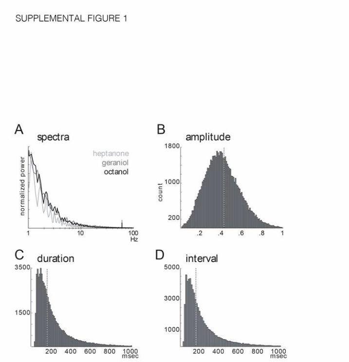
Supplemental Figure 1. Turbulent odor plume statistics. Related to Figure 1.
Turbulent plume characteristics, measured from EAG recordings.
A. Power spectra from unfiltered EAG records for 3 odorants. Each data line is from a
different experiment, and represents the mean spectra from 5, 30sec recordings. Note
that most power is below 5Hz.
B-D. Detected filaments (see Methods) were distributed in amplitude (B, shown:
normalized), duration (C), and interval (D). Dotted vertical line: median. These filaments
underlie the deflections characterized by the unfiltered power spectra. Deflection
statistics for each experiment are based upon deflections that exceeded EAG baseline
variance prior to odorant placement in the wind tunnel (see Methods).
Supplemental Figure 2. Characterizing the odor plume used in the behavioral
experiments. Related to Experimental Procedures.
a. Diagram illustrating the layout of the video frame in B, above view of the odor delivery
tube and odor plume.
b. Video frame taken while passing smoke through the odor path. The odor/smoke
plume can be seen as a diagonal white line in the image.
c. Diagram illustrating the layout of the composite image in d. A tightly packed lattice of
air sources is used with a laminar jet of clean air simultaneously flowing from each air
source. Flow-matched odorized air can be added to two of these jets, one at the top and
one at the bottom.
Houston, Stopfer, Cassenaer, Aldworth and Laurent
6
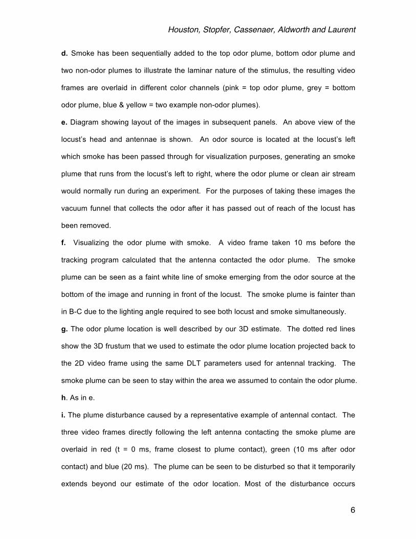
d. Smoke has been sequentially added to the top odor plume, bottom odor plume and
two non-odor plumes to illustrate the laminar nature of the stimulus, the resulting video
frames are overlaid in different color channels (pink = top odor plume, grey = bottom
odor plume, blue & yellow = two example non-odor plumes).
e. Diagram showing layout of the images in subsequent panels. An above view of the
locust’s head and antennae is shown. An odor source is located at the locust’s left
which smoke has been passed through for visualization purposes, generating an smoke
plume that runs from the locust’s left to right, where the odor plume or clean air stream
would normally run during an experiment. For the purposes of taking these images the
vacuum funnel that collects the odor after it has passed out of reach of the locust has
been removed.
f. Visualizing the odor plume with smoke. A video frame taken 10 ms before the
tracking program calculated that the antenna contacted the odor plume. The smoke
plume can be seen as a faint white line of smoke emerging from the odor source at the
bottom of the image and running in front of the locust. The smoke plume is fainter than
in B-C due to the lighting angle required to see both locust and smoke simultaneously.
g. The odor plume location is well described by our 3D estimate. The dotted red lines
show the 3D frustum that we used to estimate the odor plume location projected back to
the 2D video frame using the same DLT parameters used for antennal tracking. The
smoke plume can be seen to stay within the area we assumed to contain the odor plume.
h. As in e.
i. The plume disturbance caused by a representative example of antennal contact. The
three video frames directly following the left antenna contacting the smoke plume are
overlaid in red (t = 0 ms, frame closest to plume contact), green (10 ms after odor
contact) and blue (20 ms). The plume can be seen to be disturbed so that it temporarily
extends beyond our estimate of the odor location. Most of the disturbance occurs
Houston, Stopfer, Cassenaer, Aldworth and Laurent
7
downstream from the antenna and quickly travels downstream from the antenna so that
it is out of reach of the antenna in 30 msec. Frames are overlaid by plotting only the
difference between each successive frame in red, green or blue respectively.
j. Video frame 30 ms after the odor contact shown in i. Smoke plume has returned to its
original position and is again well described by our estimate of its location as in g.
Supplemental Video 1 - Example behavioral response to odor. Related to Figure 6.
Above view of a tethered locust walking on a ball. The animal’s head, antennae and
forelegs can be seen. At the start of the video a clean laminar air stream is presented
from the locust’s left, denoted by the blue arrow. Halfway through the video, odor is
added to the air stream, denoted by the red arrow. Upon presentation of odor, the locust
probes the area to its left with its antennae and starts turning to the left with its legs.
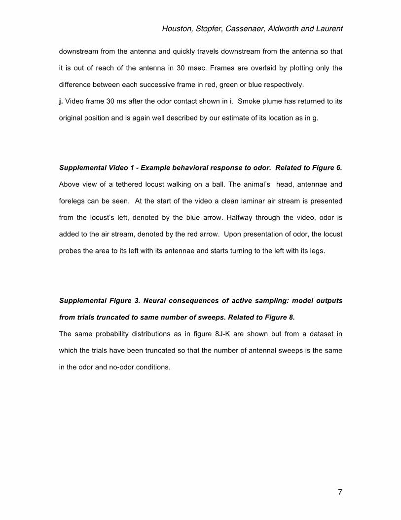
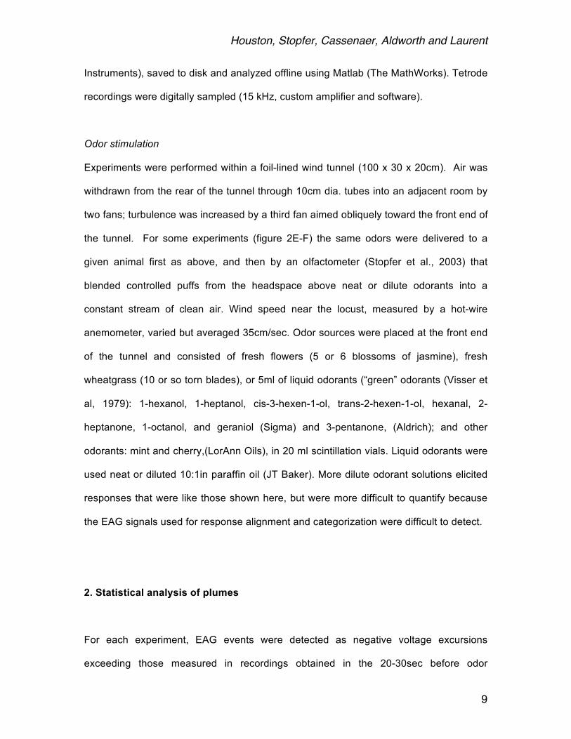
Supplemental Figure 3. Neural consequences of active sampling: model outputs
from trials truncated to same number of sweeps. Related to Figure 8.
The same probability distributions as in figure 8J-K are shown but from a dataset in
which the trials have been truncated so that the number of antennal sweeps is the same
in the odor and no-odor conditions.

Houston, Stopfer, Cassenaer, Aldworth and Laurent
8
Supplemental Experimental Procedures
1. Odor plume experiments
Animals
Results were obtained from 83 locusts (Schistocerca americana) of both sexes from a
crowded colony. Animals were immobilized with one antenna intact; the other antenna
was removed, placed parallel to and within 3 mm of the intact antenna, and used to
record EAGs (see below). The brain was exposed, de-sheathed, and superfused with
locust saline, as previously described (Laurent and Davidowitz, 1994; Stopfer et al,
2003).
Electrophysiology
EAGs were recorded using chlorided silver wire electrodes (0.1mm dia., WPI) placed
into both ends of an isolated antenna, held with small drops of wax (Vickers et al., 2001),
and wired to a DC amplifier (Brownlee). Intracellular recordings from antennal lobe
neurons were made using sharp glass micropipettes (150-350MΩ, Sutter P87 horizontal
puller) filled with 0.5M K acetate, amplified by DC amplifier (Axon Instruments). All KCs
and some PNs (Fig 2E,F) and LFPs (Figs. 2,3,5) were recorded using custom twisted-
wire tetrodes or silicone probes provided by the University of Michigan. Multiunit
recordings were analyzed offline using the Spike-O-Matic algorithm (Pouzat et al., 2002;
http://www.biomedicale.univ-paris5.fr/SpikeOMatic/) implemented in Igor (Wavemetrics).
Some LFPs (Figs. 2A,B) were recorded using saline-filled blunt glass micropipettes
(~10µm tips, 10-15MΩ), amplified by a separate DC amplifier (Axon Instruments).
Intracellular recording data were digitally sampled (2 kHz) (LabView software, National
Houston, Stopfer, Cassenaer, Aldworth and Laurent
9
Instruments), saved to disk and analyzed offline using Matlab (The MathWorks). Tetrode
recordings were digitally sampled (15 kHz, custom amplifier and software).
Odor stimulation
Experiments were performed within a foil-lined wind tunnel (100 x 30 x 20cm). Air was
withdrawn from the rear of the tunnel through 10cm dia. tubes into an adjacent room by
two fans; turbulence was increased by a third fan aimed obliquely toward the front end of
the tunnel. For some experiments (figure 2E-F) the same odors were delivered to a
given animal first as above, and then by an olfactometer (Stopfer et al., 2003) that
blended controlled puffs from the headspace above neat or dilute odorants into a
constant stream of clean air. Wind speed near the locust, measured by a hot-wire
anemometer, varied but averaged 35cm/sec. Odor sources were placed at the front end
of the tunnel and consisted of fresh flowers (5 or 6 blossoms of jasmine), fresh
wheatgrass (10 or so torn blades), or 5ml of liquid odorants (“green” odorants (Visser et
al, 1979): 1-hexanol, 1-heptanol, cis-3-hexen-1-ol, trans-2-hexen-1-ol, hexanal, 2-
heptanone, 1-octanol, and geraniol (Sigma) and 3-pentanone, (Aldrich); and other
odorants: mint and cherry,(LorAnn Oils), in 20 ml scintillation vials. Liquid odorants were
used neat or diluted 10:1in paraffin oil (JT Baker). More dilute odorant solutions elicited
responses that were like those shown here, but were more difficult to quantify because
the EAG signals used for response alignment and categorization were difficult to detect.
2. Statistical analysis of plumes
For each experiment, EAG events were detected as negative voltage excursions
exceeding those measured in recordings obtained in the 20-30sec before odor

Houston, Stopfer, Cassenaer, Aldworth and Laurent
10
stimulation. For display, EAGs were band-pass filtered (5-50Hz) by a noncausal
algorithm to remove noise and slow drift. For the LFP analysis described in Fig. 3B, two
threshold levels (the symmetrical upper and lower tails of the distribution of EAG sample
point values) were used by an automated algorithm. High values were classified as “flat;”
low values were classified as “peak.” A range of threshold levels (5% – 40%) was tried;
all gave similar results; for data presented here, threshold levels were upper and lower
20%. Once EAG events were identified, a brief temporal offset was selected to
compensate for the spatial separation between the isolated (EAG) and intact antennae;
this single offset value was used to analyze all deflections in a given experiment. The
resulting EAG event onset times were used to trigger subsequent analyses. Spectral
power was measured in an unfiltered 256msec LFP window aligned to the onset of each
“peak” and “flat” feature. Coherence estimates: PN spike rasters were convolved with a
15ms Gaussian; the resulting continuous waveforms were compared to the
corresponding bandpass-filtered (5-55Hz, non-causal) LFPs using a multitaper method
implemented in Matlab. Statistical comparisons: each experiment consisted of several
trials; results were averaged to yield a single score per experiment; thus, for LFP
comparisons (figs. 3B and 5F,G), n=22 experiments. Classification analysis: For each
experiment, EAG-deflection aligned multiunit PN spike trains were binned (50ms) and
assembled into vectors of length (bins x cells). Different numbers of bins were included
in the analysis (Fig. 4A, abscissa). Five odors were used. Euclidean distances between
each high-dimensional vector and the centroid of all vectors (centroid leaving out the
vector being compared) were measured. Classification succeeded when the distance
was least for odor-matched vectors and centroids. In some cases (Fig. 4A, 1 group) all
deflection-aligned patterns were included in the analysis; in other cases (Fig. 4A,
separate quintiles), EAG deflections were first sorted by amplitude into quintiles, and
classification was then performed using only patterns corresponding to deflections within

Houston, Stopfer, Cassenaer, Aldworth and Laurent
11
each quintile. For classification by Gaussian mixture model (GMM, Fig. 4B-D),
population responses to a set of odors consisted of PN-firing-rate vectors binned at 20
Hz (the approximate frequency of synchronous oscillations within the antenna lobe) and
projected into a 2- or 3-dimensional principal component subspace (Stopfer et al, 2003,
Brown et al, 2005, Mazor & Laurent, 2005). Model size was limited to the first 500ms (10
samples at 20Hz) following onset of the response to the odor pulse.. To decode this
information, pairs of models derived from presentations of two different odorants in a
given experiment were combined into a Gaussian mixture model (GMM), with the priors
adjusted so that posterior probabilities from the two models were equivalent when
presented with responses of PNs to clean air. KC odor specificity (Fig. 5C), was
assessed with a series of 4 or 5 odorants, each presented both as controlled pulses and
as plumes. Of all spikes counted in each KC, we determined the percentage elicited by
each of the odors under both presentation conditions. All statistical tests were 2-tailed.
3. Active sampling experiments
Animal selection - behavior experiments
Schistocerca americana reared in crowded conditions and fed on wheat grass seedlings
were used for all experiments. At any one time, the majority of locusts in the colony
cage were in a quiescent state with reduced locomotor activity and no obvious
behavioral response to odors. For our experiments we pre-screened for animals that
were actively seeking food. Females who had gone through their final molt in the past
week were starved overnight. These locusts were then placed in an empty cage with a
trap containing crushed wheat grass odor for 5-15 mins. Only those locusts that entered
the trap were used. In total, data from 14 locusts was used for the behavioral

Houston, Stopfer, Cassenaer, Aldworth and Laurent
12
experiments and 8 locusts for the simultaneous electrophysiology and behavior
experiments.
Head-fixed female locusts with painted eyes were tethered to a post and placed on a
hollow Styrofoam ball so they could walk and move their antennae freely. The animal’s
walking behavior was tracked by the rotation of the ball across all 3 degrees of freedom
and the 3D position of the antennae were monitored by 3 video views at roughly
orthogonal angles and were analyzed by a custom-written antenna tracking algorithm
(see Supplemental Methods). Thin (~1 mm in diameter) stable laminar air streams were
placed within reach of the antennae such that the antennae were free to sweep in and
out of them. During odor delivery, flow-matched crushed wheat grass odor or cis-3-
hexen-1-ol was added to one of the air streams. For a given experiment, one of two
stimulus configurations was used. To test odor delivery from the left or right of a locust,
air streams were simultaneously present at both the locust’s left and right (figure 1G).
The air streams were angled so as to not intersect. To test odor delivery from above or
below the locust, a tight lattice of multiple laminar air streams was constructed and odor
was added to either a high or low airstream within this lattice (Fig 1H, SI Fig 1C-D). In
this way there was no change in airflow rate as the antenna passed from outside the
odor stream into it. All stimuli were calibrated by passing smoke through the air source
and reconstructing the stimulus position in 3D (supplemental Fig 3). Each trial consisted
of 10 s of a clean air run through the airstream of interest, followed by 10 s of odor,
followed by 10 s of clean air.
Tethering
Locusts’ eyes and ocelli were painted with non-toxic black paint to remove visual cues.
The head was fixed to the body in a neutral position with care taken to leave the

Houston, Stopfer, Cassenaer, Aldworth and Laurent
13
mouthparts unobstructed. The locusts were tethered to a post at their pronotum and
placed above a hollow 6.35 cm diameter, 2.8 g polystyrene ball in a position where they
could walk on the ball at an angle as close to their natural walking posture as possible.
A heat lamp was placed 1 m in front of the locust to encourage it to walk forward. The
air temperature directly next to the locust was continually monitored. If the temperature
fell outside a range of 28-34 degrees Celsius the experiment was halted until the
temperature returned to the acceptable range.
Measuring walking
The locust’s walking direction and speed were monitored using a trackball system similar
to that described by Hedwig & Poulet (2005). In brief, the ball’s rotation was monitored
by an optical mouse sensor chip (Agilent ADNS-2051) in a custom circuit with the sensor
placed behind a lens (EC-ML8 Elyssa Corp) to give it a longer working distance.
Another custom circuit decoded the chip’s quadrature output into a series of pulses, the
frequency of which were proportional to the rotational speed of the ball around a
particular axis. Each sensor monitored two axes of ball rotation, so by using two
sensors we monitored all three axes of rotation of the ball.
The motion sensors were calibrated by mounting the ball on a motor and rotating it at
different speeds around different axes. The sensors provided a linear output with
respect to the ball’s rotation frequency across the measured range of 0.05 to 1 Hz,
corresponding to a walking speed of 1-20 cm/sec, which easily spanned the range of
locust walking speeds. As the ball’s axis of rotation moved away from a motion
detector’s preferred axis, its output pulse rate decreased in a cosine manner allowing us
to combine outputs of multiple sensors to reconstruct the ball’s true axis and speed of
rotation and thus the locust’s walking speed and direction. The motion detectors had a
Houston, Stopfer, Cassenaer, Aldworth and Laurent
14
frame rate of 1500 fps, allowing us to resolve individual footsteps of the locust. The
pulsed outputs of the trackball system were sampled at 15500 Hz by a National
Instruments A/D board controlled by Matlab. For further analysis the pulsed outputs
were filtered offline with a Gaussian with a standard deviation of 50 msec.
Odor stimuli
Stable laminar air streams approximately 1 mm in diameter were generated within reach
of the locust’s antenna such that the locust was free to sweep its antenna in and out of
the air stream, but not able to reach the air source. Air was passed through 0.5 - 2 mm
diameter tubes at 44-130 ml/min. After travelling 3-5 cm from the tube outlet, the air
stream was collected by a small funnel connected to a vacuum trap. At the start of each
experiment the flow rate was fine-tuned while passing smoke through the air stream to
ensure that it was laminar for the short distance from source to vacuum trap, but moving
fast enough that local air currents did not cause it to drift. Smoke was passed through
the air stream again at the end of the experiment to ensure the stream was still laminar
and at the same location. All stimuli had a Reynolds number in the range 50-400 within
the delivery tube, well within the laminar range. To calculate when the locust antennae
contacted odor, we needed an accurate estimate of where the odor plume was in 3D.
Using video of the smoke filled airstream and the same 3D calibration that we used for
tracking the antennae (see later), we defined the 3D frustum (truncated cone) of space
that the airstream/odor occupied. The accuracy of this frustum was not only confirmed
by back projecting the 3D frustum to the 2D videos of the smoke-filled plume (e.g.
supplemental figure 2g), but also by later analysis of the neural data, which only showed
odor-induced responses when the antenna was within the region we defined as
containing odor (e.g. figure 8E).

Houston, Stopfer, Cassenaer, Aldworth and Laurent
15
Even though the airstream remained stable when undisturbed, it was still interrupted
when the locust antenna passed through the airstream. To characterize this we filmed
the smoke filled air stream while a locust was free to pass its antenna in and out of the
air stream. When the antenna passed through the airstream the downstream structure
was briefly interrupted - often widening slightly. However, it was extremely rare for the
other antenna to be within a region downstream that could contact the widened
airstream for the short period in which it was altered, so this disruption had minimal
effect on our data. Often as the antenna left the airstream it shed a small vortex
containing smoke/odor that then travelled downstream away from the antenna and
towards the vacuum trap (supplemental figure 2i). Due to the fast stimulus airflow these
vortices travelled out of reach of the locust’s antenna within approximately 3 frames or
30 ms (supplemental figure 2j) and were then removed by the vacuum trap so we do not
believe they significantly affected our data.
One of two stimulus configurations was used to test the locust’s sensitivity to left vs. right
or high vs. low odor sources. For the left-right configuration, two air streams were
simultaneously present, one from the locust’s left and one from the right (figure 1G).
The air streams were angled slightly so that they did not intersect with each other. Flow-
matched odorized air was added to either the left or right airstream. For the high-low
configuration a lattice of 34 air streams each with the same flow rate was presented from
the locust’s left (figure 1H & supplemental figure 2c-d). A flow rate matched odor stream
was added to one of the air streams within the lattice either at the top or the bottom of
the lattice (figure 1H & supplemental figure 2c-d). In this configuration, the odor plume
was embedded in a flow-matched laminar air stream such that the transition between
odor and clean air was not accompanied by a change in airflow rate.
Houston, Stopfer, Cassenaer, Aldworth and Laurent
16
For the behavioral experiments we used odor from crushed wheat grass, the food
source provided in the locust’s rearing cages. We crushed the grass as locusts have
been observed to more readily respond to the odor of plants damaged during
consumption by other locusts than to that of undamaged plants (reviewed in Byers 1991).
Five grams of wheatgrass seedlings were cut, crushed and rubbed against lab tissue
paper. Air was passed directly through the grass-scented tissue paper before reaching
the odor stimulus port. For the control (non-odor) trials, the same tissue paper was used
but without being rubbed on the grass. The grass scented tissue was replaced every 5
trials. To enable more control over the odorant concentration in the electrophysiology
experiments, we used 5 ml of neat liquid odorant cis-3-hexen-1-ol (Sigma). The liquid
odorant was placed in a small vial and air was passed through the vial before reaching
the odor stimulus port, control stimuli were passed through an empty vial. Cis-3-hexen-
1-ol is a major component of the odor released by damaged grasses (Kirstine et al.
1998) and other leafy plants (reviewed in Hatanaka, 1993) and has been shown to be
attractive to grasshoppers (Hopkins & Young 1990). We also performed one
electrophysiology experiment using both the crushed grass odor and cis-3-hexen-1-ol,
the results were similar for both odors.
Each trial was 30 seconds long, consisting of 10 seconds of no odor where all clean air
streams were present, followed by 10 s where one of the clean air streams was replaced
with an odorized one of the same flow rate, followed by 10s of no odor. The odor tubes
were thoroughly flushed with clean air between each trial. The timing of the odor
stimulus was synchronized with other data sources by recording the TTL command
pulse that triggered opening and closing of the odor valve. No trials were detected
where the locusts’ antennae were touching the air stream at the time of the odor onset or
offset transient.

Houston, Stopfer, Cassenaer, Aldworth and Laurent
17
Electrophysiological recordings in tethered animals
For simultaneous electrophysiology and behavior experiments, the locusts were tethered
as described above. The left antenna was removed and a hole was cut in the cuticle to
expose the brain. The foregut was ligatured and removed and the brain was supported
on a custom made platform to reduce movement. Extra care was taken to minimize brain
movement and to avoid interference with the antennal muscles or the antenna itself such
that the right antenna was free to move naturally during our electrophysiology recordings.
Sharp 130 MΩ borosilicate electrodes were filled with 1M K acetate and used to record
from the projection neurons in the antennal lobe. LFP signals were recorded in the
mushroom body using multi-channel silicon probes (University of Michigan center for
Neural Communication Technology) whose outputs were band-pass filtered between 1
and 300 Hz; recordings were accepted only if no movement artifacts was observed in
the 5-55 Hz range during spontaneous antennal movements. Sliding-window auto-
correlation was computed on 5-55 Hz BP-filtered LFP (150ms window, 50ms step).
Sliding-window cross-correlations were computed on 5-55 Hz BP-filtered LFP and 0.1Hz
high-pass filtered PN recordings; they were triggered on antennal crossings of the odor
stream and averaged over odor stream crossing events.
Video acquisition
Video of the locust was recorded from above at 100 fps with a resolution of 468x490
(Basler a602f camera). Image acquisition was controlled through Matlab. Illumination
was provided by an array of red LEDs (Thor Labs). Two mirrors were placed either side
of the locust at approximately 45 degree angles such that the video image contained 3
different views of the locust: one from above and one from each side of the locust. Thus,
we recorded two approximately orthogonal views of each antenna allowing us to

Houston, Stopfer, Cassenaer, Aldworth and Laurent
18
reconstruct its position in 3D using the Direct Linear Transform method (DLT, Abdel-Aziz
and Karara 1971). Parameters of the DLT were estimated at the start and end of each
experiment by videoing and digitizing a calibration object in all 3 fields of view (mean
DLT residual = 2 mm).
Camera frames were synchronized with the trackball and electrophysiology data by
triggering each camera frame with a TTL pulse and recording the timing of the pulse
through the same A/D board as the trackball and electrophysiology data. This
synchronization was confirmed in separate experiments by driving an LED in the video
field of view with the camera command pulse and analyzing the resulting images offline.
Antennal tracking
We used a semi-automated program custom written in Matlab to track the position of the
locust’s antennae in 3D. The antennae were first tracked individually in each of the
three 2D views. Candidate 2D line segments were detected by finding peaks in a Hough
transform that was masked to only include lines that pivoted around the locust’s antennal
base. The antennal position was automatically selected from the candidate line
segments using information about its previous position and velocity. The same 2D
tracking method was run over the video forwards, backwards and over images derived
from individual frames and images derived from the difference between successive
frames. Any discrepancies between these multiple runs were resolved by a set of hand-
tuned rules designed to choose the result least likely to be an error. The 2D tracking
results were then combined to produce a 3D estimate of the antennal location using the
DLT. Errors in tracking were easily automatically detected at this stage by detecting
changes in the reconstructed antennal length or peaks in the DLT residuals. The
program first attempted to automatically resolve these errors by returning to the set of

Houston, Stopfer, Cassenaer, Aldworth and Laurent
19
2D candidate lines and picking a new set. If the program was unable to resolve the
errors, it returned them to the user for hand-digitization of those video segments.
To estimate the accuracy of the tracking algorithm we chose a sample (16-s long, 1600
frames) of video to compare the automatic tracking output to the result of manual
digitization. The most challenging video data was used for this comparison - that from
the electrophysiology experiments where multiple thin, antenna-like, electrodes are
present. The difference between the two methods of estimating 3D antennal tip position
had a median value of 0.4 mm with an interquartile range of 0.4 mm corresponding to an
error of 1.6 degrees in estimating tip angular position.
4. Electrophysiology
Dissection
For the electrophysiology experiments the locusts were tethered as described above.
The gut was then removed and the tip of the abdomen lightly tied with thread. The left
antenna was removed and a small hole cut in the cuticle exposing the brain, but making
sure not to disturb the cuticle around the right antennal base or the antennal muscles,
leaving the right antenna free to move normally. The hole was surrounded by a minimal
beeswax border, big enough to prevent saline spillage but shaped so as to not interfere
with the antennal movements. A platform constructed from beeswax and steel wire was
placed under the brain, and extra care was taken to stabilize any brain movements. The
right antennal lobe and/or mushroom body were then desheathed (See Laurent and
Naraghi, 1994 for more details).
Houston, Stopfer, Cassenaer, Aldworth and Laurent
20
Intracellular recordings
Sharp 130 MΩ borosilicate electrodes were filled with 1M Potassium Acetate. External
saline was as in Laurent and Naraghi, (1994). Recordings were made from the
Projection Neurons of the antennal lobe, amplified by a DC amplifier and sampled at
15500 Hz by an A/D board.
Local Field Potential (LFP) recordings
LFP signals were recorded using multichannel silicon probes (University of Michigan
Center for Neural Communication Technology) amplified by a custom amplifier, band-
pass filtered between 1 and 300 Hz and sampled at 15500 Hz by an A/D board. Before
starting the experiment, LFP recordings were observed during antennal movements in
clean air and the recordings were only accepted if there were no motion artifacts visible
in the 5-55 Hz frequency range. Continuous time series of LFP power were calculated
using a sliding Hamming window with a width 2 x the period of the lowest frequency in
the band of interest and a 10-ms step size.
5. Data analysis
Antennal sweeps were detected by finding peaks in the time series of the antennal tip
elevation. Odor contacts were estimated by interpolating the 100-Hz samples of
antennal kinematics to 1000 Hz and computing when the antenna intersected the 3D
frustum describing the odor stream.
Behavioral latency

Houston, Stopfer, Cassenaer, Aldworth and Laurent
21
We identified the antennal sweep that resulted in the first odor contact in each trial.
Behavioral latency was estimated by comparing the kinematics of these antennal
sweeps to the kinematics of equivalent sweeps that contacted the clean air stream just
prior to odor onset. These two sets of sweep kinematics were zeroed to the time of
initial odor or clean air stream contact and then pooled for all trials to give a distribution
of sweeps for the no-odor (blue, figure 7F) and initial odor contact conditions (red, figure
7F). The two sweep distributions were normalized to enable pooling of data from
different locusts. The two sweep distributions remained statistically indistinguishable
until the point of initial odor/clean airstream contact. After odor contact the two sweep
distributions started to separate, the odor contact sweeps having a lower elevation on
average reflecting the tendency of the sweeps to have a lower top inflection point when
the locust detected odor. We quantified when, after initial odor contact, the sweep
elevation kinematics first statistically diverged from those of the sweeps before odor
contact. For each time point we performed a two-sided Wilcoxon rank-sum test that the
antennal tip elevations come from distributions with the same medians. The resulting p-
values were subjected to False Detection Rate (FDR) correction to compensate for
multiple tests. Plotting the corrected p-values over time showed that the two sweep
distributions remained statistically indistinguishable until around 130 ms after odor
contact when the p-values started to fall dramatically (figure 7G). We defined the
behavioral latency as the time from odor contact to the time at which the probability that
the odor and no-odor sweep distributions were the same was less than 5% (horizontal
dotted line in figure 7G).
Measuring LFP information about odor location
We plotted antennal tip position in coordinates of azimuth and elevation relative to the
antennal base (2x2 degree bins) and color coded each antennal tip position by the
Houston, Stopfer, Cassenaer, Aldworth and Laurent
22
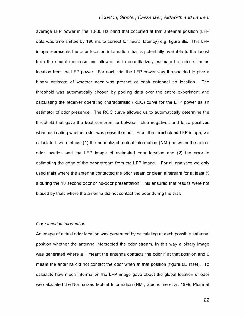
average LFP power in the 10-30 Hz band that occurred at that antennal position (LFP
data was time shifted by 160 ms to correct for neural latency) e.g. figure 8E. This LFP
image represents the odor location information that is potentially available to the locust
from the neural response and allowed us to quantitatively estimate the odor stimulus
location from the LFP power. For each trial the LFP power was thresholded to give a
binary estimate of whether odor was present at each antennal tip location. The
threshold was automatically chosen by pooling data over the entire experiment and
calculating the receiver operating characteristic (ROC) curve for the LFP power as an
estimator of odor presence. The ROC curve allowed us to automatically determine the
threshold that gave the best compromise between false negatives and false positives
when estimating whether odor was present or not. From the thresholded LFP image, we
calculated two metrics: (1) the normalized mutual information (NMI) between the actual
odor location and the LFP image of estimated odor location and (2) the error in
estimating the edge of the odor stream from the LFP image. For all analyses we only
used trials where the antenna contacted the odor steam or clean airstream for at least ⅓
s during the 10 second odor or no-odor presentation. This ensured that results were not
biased by trials where the antenna did not contact the odor during the trial.
Odor location information
An image of actual odor location was generated by calculating at each possible antennal
position whether the antenna intersected the odor stream. In this way a binary image
was generated where a 1 meant the antenna contacts the odor if at that position and 0
meant the antenna did not contact the odor when at that position (figure 8E inset). To
calculate how much information the LFP image gave about the global location of odor
we calculated the Normalized Mutual Information (NMI, Studholme et al. 1999, Pluim et

Houston, Stopfer, Cassenaer, Aldworth and Laurent
23
al. 2003) between the thresholded LFP image and the actual odor location image. Using
a mutual information measure takes into account that, due to odor locations being rarer
than the lack of odor, detecting the presence of odor at a given location is more
informative about global odor location than detecting the absence of odor. Using NMI
instead of standard mutual information allows comparison between images with varying
degrees of overlap (Studholme et al. 1999, Pluim et al. 2003), which enables us to
compare data from different locusts where the antennal search envelope was of different
absolute sizes. NMI is defined by:
Where H(stimulus) is the Shannon entropy of the binary image that gives the actual odor
location, H(lfp) is the entropy of the binary image describing the locations where the LFP
power was above threshold and H(stimulus,lfp) is the joint entropy of the stimulus and
LFP images. Locations in the LFP image that were not visited by the antenna were
randomly set to zero or one with a probability that matched the probability of the
occurrence of odor pixels in the stimulus image, reflecting that unsampled areas gave
zero information about the odor location. A NMI of 0 means that the LFP image
contained zero information about the odor stimulus location, a NMI of 1 means that the
LFP image perfectly reconstructed the location of odor and no-odor at all points
surrounding the locust.
Odor edge estimation
In the behavioral experiments locusts shifted their antennal search patterns to center on
the edge of the odor stream (figure 6M,N), thus providing more samples of that area.
Houston, Stopfer, Cassenaer, Aldworth and Laurent
24
We quantified the extent to which this increase in sampling of the odor edge meant the
LFP provided a better signal from which to estimate the location of the odor edge and
thus the direction in which to walk to find the odor source. To do this we used the LFP
image to estimate the location of the odor edge. The odor edge location was estimated
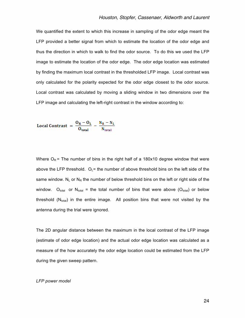
by finding the maximum local contrast in the thresholded LFP image. Local contrast was
only calculated for the polarity expected for the odor edge closest to the odor source.
Local contrast was calculated by moving a sliding window in two dimensions over the
LFP image and calculating the left-right contrast in the window according to:
Where OR = The number of bins in the right half of a 180x10 degree window that were
above the LFP threshold. OL= the number of above threshold bins on the left side of the
same window. NL or NR the number of below threshold bins on the left or right side of the
window. Ototal or Ntotal = the total number of bins that were above (Ototal) or below
threshold (Ntotal) in the entire image. All position bins that were not visited by the
antenna during the trial were ignored.
The 2D angular distance between the maximum in the local contrast of the LFP image
(estimate of odor edge location) and the actual odor edge location was calculated as a
measure of the how accurately the odor edge location could be estimated from the LFP
during the given sweep pattern.
LFP power model

Houston, Stopfer, Cassenaer, Aldworth and Laurent
25
To compare how different sweep patterns affect LFP responses we developed a simple
model to estimate what the LFP power response would be to an arbitrary sequence of
odor contacts. We estimated the transfer function between the odor contact time series
(estimated from antennal position and known odor location) and the 10-30 Hz LFP
power that occurred in the electrophysiology experiments. The transfer function was
estimated by dividing the average stimulus-LFP cross-correlation by the average
stimulus autocorrelation. To estimate noise, we found the average power spectral
density of the LFP power during the no-odor portions of the trials. To simulate the LFP
power response to an arbitrary sequence of odor contacts we convolved the odor
contact time series with the transfer function and then added white noise that had been
filtered by the average noise power spectrum. We verified this model by using it to
generate LFP traces for those trials where we had recorded the actual LFP from the
locust and then compared the NMI values resulting from the real LFP and the model LFP
(figure 8I).

Houston, Stopfer, Cassenaer, Aldworth and Laurent
26
Supplemental References
Abdel-Azziz, Y. I., & Karara, H. M. (1971). Direct linear transformation from comparator
coordinates into object space coordinates in close-range photogrammetry. In
Papers from the 1971 ASP Symposium on Close-range Photogrammetry (pp. 1–
18).
Byers, J. a. (1991). Pheromones and Chemical Ecology of Locusts. Biological Reviews,
66, 347–378. doi:10.1111/j.1469-185X.1991.tb01146.x
Hatanaka, A. (1993). The biogeneration of green odour by green leaves.
Phytochemistry. doi:10.1016/0031-9422(91)80003-J
Hopkins, T. L., & Young, H. (1990). Attraction of the grasshopper, Melanoplus
sanguinipes, to host plant odors and volatile components. Entomologia
Experimentalis et Applicata, 56, 249–258. doi:10.1007/BF00163696
Kirstine, W., Galbally, I., Ye, Y., & Hooper, M. (1998). Emissions of volatile organic
compounds (primarily oxygenated species) from pasture. Journal of Geophysical
Research. doi:10.1029/97JD03753
Laurent, G., & Naraghi, M. (1994). Odorant-induced oscillations in the mushroom bodies
of the locust. The Journal of Neuroscience : The Official Journal of the Society for
Neuroscience, 14, 2993–3004.
Pluim, J. P. W., Maintz, J. B. A. A., & Viergever, M. A. (2003). Mutual-information-based
registration of medical images: A survey. IEEE Transactions on Medical Imaging.
doi:10.1109/TMI.2003.815867
Houston, Stopfer, Cassenaer, Aldworth and Laurent
27
Poulet, J. F. A., & Hedwig, B. (2005). Auditory orientation in crickets: pattern recognition
controls reactive steering. Proceedings of the National Academy of Sciences of the
United States of America, 102, 15665–15669. doi:10.1073/pnas.0505282102
Studholme, C., Hill, D. L. G., & Hawkes, D. J. (1999). An overlap invariant entropy
measure of 3D medical image alignment. Pattern Recognition. doi:10.1016/S0031-
3203(98)00091-0