Neuroevolutionary design of control strategy of a multi ...
61
Transcript of Neuroevolutionary design of control strategy of a multi ...


ii
Czech Technical University in PragueFaculty of Electrical Engineering
Department of Cybernetics
Bachelor’s Thesis
Neuroevolutionary design of control strategy of a multi-leggedrobot
Jan Dvorský
Supervisor: Ing. Jiří Kubalík, Ph.D.
Study Programme: Cybernetics and Robotics
Field of Study: Robotics
May 21, 2013

iv
AknowledgementsMy greatest thanks goes to Dr. Jiri Kubalik for guiding me through the uneasy processof writing this paper. He used his experience and wit to help me overcome all the issues Iencountered. I would like to thank Mr. Jan Drchal and Mr. Jan Cerny for always havingtime for my questions when I came by their offices uninvited. A mention goes to Dr. JeffClune of University of Wyoming whom I bombarded with questions during the developmentand he found time to reply. I also appreciate the help of Mr. Vojta Vonasek and Mr. DanielFiser, who assisted me with the robotic simulator. In addition, I would like to thank Ms.Lucie Kratochvil for proof-reading and correcting my work, Mr. Vojtech Micka for helpingme look at things from different angles, Ms. Marketa Stonova for being so incredibly patientwith me and my dearest parents for always listening and supporting my dreams.

v
Abstract
This paper searches for better solutions of the robot locomotion problem. Our method isbased on the well established HyperNEAT algorithm, where we exchange NEAT with geneticprogramming. We present the resulting algorithm, construct proof-of-concept experimentsand show experimental results. In the end we offer possible future improvements to HyperGPand share the implemented testing framework with the community.
Abstrakt
Tato práce se zaměřuje na hledání lepších řešení problému robotické chůze. Naše metodaje založena na známém algoritmu HyperNEAT, kde vyměníme NEAT za genetické pro-gramování. Představíme výsledný algoritmus, provedeme experimenty a ukážeme jejichvýsledky. Nakonec navrhneme možná vylepšení algoritmu HyperGP a uvolníme náš testovacíframework komunitě.
vi
Contents
1 Introduction 1
2 Robot locomotion problem and existing methods 32.1 EANT2 - Evolutionary Acquisition of Neural Topologies, Version 2 . . . . . . 32.2 CPG - Complex motor patter generation (Rodney) . . . . . . . . . . . . . . . 32.3 HyperNEAT - Neuro-Evolution of Augmented Topologies employing hypercube-
based encoding . . . . . . . . . . . . . . . . . . . . . . . . . . . . . . . . . . . 4
3 HyperNEAT and Genetic Programming 53.1 Generative encoding . . . . . . . . . . . . . . . . . . . . . . . . . . . . . . . . 53.2 Genetic operators . . . . . . . . . . . . . . . . . . . . . . . . . . . . . . . . . . 63.3 Phenotype: substrate . . . . . . . . . . . . . . . . . . . . . . . . . . . . . . . . 73.4 Genotype: CPPN . . . . . . . . . . . . . . . . . . . . . . . . . . . . . . . . . . 73.5 Genetic Programming (GP) . . . . . . . . . . . . . . . . . . . . . . . . . . . . 9
4 Robotic simulator Sim 10
5 Proposed HyperGP approach 135.1 HyperGP . . . . . . . . . . . . . . . . . . . . . . . . . . . . . . . . . . . . . . 13
5.1.1 Initial population . . . . . . . . . . . . . . . . . . . . . . . . . . . . . . 145.1.2 Selection . . . . . . . . . . . . . . . . . . . . . . . . . . . . . . . . . . . 145.1.3 Mutation . . . . . . . . . . . . . . . . . . . . . . . . . . . . . . . . . . 145.1.4 Recombination . . . . . . . . . . . . . . . . . . . . . . . . . . . . . . . 145.1.5 Evaluation . . . . . . . . . . . . . . . . . . . . . . . . . . . . . . . . . . 155.1.6 Termination condition . . . . . . . . . . . . . . . . . . . . . . . . . . . 15
5.2 Bloat control . . . . . . . . . . . . . . . . . . . . . . . . . . . . . . . . . . . . 155.2.1 Heavy variant . . . . . . . . . . . . . . . . . . . . . . . . . . . . . . . . 165.2.2 Handling illegals . . . . . . . . . . . . . . . . . . . . . . . . . . . . . . 165.2.3 Very Heavy variant . . . . . . . . . . . . . . . . . . . . . . . . . . . . . 16
6 Implementation 176.1 Programming environment . . . . . . . . . . . . . . . . . . . . . . . . . . . . . 17
6.1.1 Programming language . . . . . . . . . . . . . . . . . . . . . . . . . . . 176.1.2 Compiler . . . . . . . . . . . . . . . . . . . . . . . . . . . . . . . . . . 186.1.3 Platform . . . . . . . . . . . . . . . . . . . . . . . . . . . . . . . . . . . 18
6.2 The cic framework . . . . . . . . . . . . . . . . . . . . . . . . . . . . . . . . . 18
vii

CONTENTS viii
6.2.1 Experiment: Symbolic Regression - cic::genetic::symreg . . . . . . . . . 206.2.2 Experiment: HyperGP - cic::genetic::hyperGP . . . . . . . . . . . . . . 21
6.3 cic featured classes . . . . . . . . . . . . . . . . . . . . . . . . . . . . . . . . . 216.3.1 cic::genetic::Individual . . . . . . . . . . . . . . . . . . . . . . . . . . . 226.3.2 cic::genetic::Population . . . . . . . . . . . . . . . . . . . . . . . . . . . 226.3.3 cic::tree::Tree . . . . . . . . . . . . . . . . . . . . . . . . . . . . . . . . 22
6.3.3.1 Node . . . . . . . . . . . . . . . . . . . . . . . . . . . . . . . 236.3.3.2 Tree . . . . . . . . . . . . . . . . . . . . . . . . . . . . . . . . 23
6.3.4 Tree Generator . . . . . . . . . . . . . . . . . . . . . . . . . . . . . . . 236.3.4.1 Grow . . . . . . . . . . . . . . . . . . . . . . . . . . . . . . . 256.3.4.2 Full . . . . . . . . . . . . . . . . . . . . . . . . . . . . . . . . 256.3.4.3 Ramped Half-and-Half . . . . . . . . . . . . . . . . . . . . . . 266.3.4.4 PTC1 . . . . . . . . . . . . . . . . . . . . . . . . . . . . . . . 26
6.3.5 cic::nn::Network . . . . . . . . . . . . . . . . . . . . . . . . . . . . . . 276.4 Tools and libraries . . . . . . . . . . . . . . . . . . . . . . . . . . . . . . . . . 29
6.4.1 libxml2 . . . . . . . . . . . . . . . . . . . . . . . . . . . . . . . . . . . 296.4.2 MATLAB . . . . . . . . . . . . . . . . . . . . . . . . . . . . . . . . . . 296.4.3 Sim . . . . . . . . . . . . . . . . . . . . . . . . . . . . . . . . . . . . . 306.4.4 Other tools . . . . . . . . . . . . . . . . . . . . . . . . . . . . . . . . . 30
7 Testing 317.1 Experimental setup . . . . . . . . . . . . . . . . . . . . . . . . . . . . . . . . . 31
7.1.1 Tested robot topologies . . . . . . . . . . . . . . . . . . . . . . . . . . 317.1.2 Fitness . . . . . . . . . . . . . . . . . . . . . . . . . . . . . . . . . . . . 32
7.2 Experimental results . . . . . . . . . . . . . . . . . . . . . . . . . . . . . . . . 327.2.1 Genotype size: 1 vs. 4 trees . . . . . . . . . . . . . . . . . . . . . . . . 327.2.2 Number of legs: 4 vs. 6 . . . . . . . . . . . . . . . . . . . . . . . . . . 357.2.3 Simulation sampling frequency . . . . . . . . . . . . . . . . . . . . . . 367.2.4 Robot topologies . . . . . . . . . . . . . . . . . . . . . . . . . . . . . . 36
7.3 Issues encountered during testing . . . . . . . . . . . . . . . . . . . . . . . . . 377.3.1 Genotype: forest instead of a tree . . . . . . . . . . . . . . . . . . . . . 377.3.2 Neural network outputs . . . . . . . . . . . . . . . . . . . . . . . . . . 38
7.3.2.1 High-frequency oscillations . . . . . . . . . . . . . . . . . . . 387.3.2.2 Neuron output saturation . . . . . . . . . . . . . . . . . . . . 40
8 Conclusion 42
A Important terms and abbreviations 47
B Experimental setup 48
C Attached CD content 51

List of Figures
3.1 Relationship of the substrate and the robot topology . . . . . . . . . . . . . . 83.2 Hypercube encoding example . . . . . . . . . . . . . . . . . . . . . . . . . . . 9
4.1 One SSSA robot . . . . . . . . . . . . . . . . . . . . . . . . . . . . . . . . . . 114.2 Many SSSA pieces forming what we refer to as a robot . . . . . . . . . . . . . 11
5.1 HyperGP derived from HyperNEAT . . . . . . . . . . . . . . . . . . . . . . . 145.2 GP evolution . . . . . . . . . . . . . . . . . . . . . . . . . . . . . . . . . . . . 15
6.1 cic types hierarchy with symreg and hyperGP . . . . . . . . . . . . . . . . . . 196.2 symreg workings in cic . . . . . . . . . . . . . . . . . . . . . . . . . . . . . . . 206.3 HyperGP workings in cic . . . . . . . . . . . . . . . . . . . . . . . . . . . . . 216.4 cic::Individual . . . . . . . . . . . . . . . . . . . . . . . . . . . . . . . . . . . . 226.5 cic::Population . . . . . . . . . . . . . . . . . . . . . . . . . . . . . . . . . . . 236.6 Example nodes connected into a tree . . . . . . . . . . . . . . . . . . . . . . . 246.7 Tree types hierarchy . . . . . . . . . . . . . . . . . . . . . . . . . . . . . . . . 246.8 Neural network - synapsis delay by type . . . . . . . . . . . . . . . . . . . . . 286.9 Recurrent neural network example - spacial view . . . . . . . . . . . . . . . . 286.10 Recurrent neural network example - layer view . . . . . . . . . . . . . . . . . 29
7.1 Robot R1 . . . . . . . . . . . . . . . . . . . . . . . . . . . . . . . . . . . . . . 337.2 Robot R2 . . . . . . . . . . . . . . . . . . . . . . . . . . . . . . . . . . . . . . 337.3 Robot R1 with 6 legs . . . . . . . . . . . . . . . . . . . . . . . . . . . . . . . . 347.4 Comparing genotypes with 1, respectively 4 trees . . . . . . . . . . . . . . . . 347.5 Comparing robots with 4, respectively 6 legs . . . . . . . . . . . . . . . . . . . 357.6 Comparing robots ran on sample time 0.5s, respectively 0.0125s . . . . . . . . 367.7 Comparing robot topologies: R0, R1 and R2 . . . . . . . . . . . . . . . . . . 377.8 Neural network outputs: High frequency oscillations - original (no averaging) 397.9 Neural network outputs: High frequency oscillations - averaging 2 consecutive
samples . . . . . . . . . . . . . . . . . . . . . . . . . . . . . . . . . . . . . . . 407.10 Neural network outputs: High frequency oscillations - averaging 4 consecutive
samples . . . . . . . . . . . . . . . . . . . . . . . . . . . . . . . . . . . . . . . 417.11 Hyperbolic tangent . . . . . . . . . . . . . . . . . . . . . . . . . . . . . . . . . 41
ix

List of Tables
B.1 Experiment parameters . . . . . . . . . . . . . . . . . . . . . . . . . . . . . . 48
x

Chapter 1
Introduction
The humans have always been intrigued by the tools their ancestors built. Many of usdevote our lives to building upon and improving those tools. When the industrial revolutionbrought the accelerated rate of inventions, the future seemed bright for the human kind.With the use of light bulbs, electric machines and combustion engines, inventors could speedup their work and many improvements have just kept coming.
The middle of 20th century brought the greatest invention of all - the computer. Underthe spotlight pointed at the unbelievably fast processing machine, the average human couldstart feeling less brilliant, or even insufficient for the modern age. The world’s fastest com-puter can now compute over 1015 floating point operations per second [34].
Even though computers have been beating us in many tasks, such as playing chess, or-ganizing data and communication, humans and most animals still have been much moresuccessful than the computers in one little ability - coordinated locomotion. Walking is sonatural to us that we do not consider it particularly difficult and that is why this one weak-ness of computers is the major objective of our work.
We will try to develop an automated system which would enable robots to learn andperform forward locomotion. This system should be independent of the robot’s size andtopology. Additionally, in order to empower the system to solve various problems, the influ-ence of the experimenter should be as low as possible.
Our approach is based on the HyperNEAT algorithm, originally developed by Ken Stan-ley and his team [32]. HyperNEAT is a neuroevolutionary method for optimizing synapticweights in a neural network. It uses generative encoding from genotype to phenotype thatenables it to encode symmetries, repetitions and other underlying motifs. Our approachuses a modification of HyperNEAT, called HyperGP, which replaces the original neuroevo-lutionary algorithm NEAT for a simpler one, genetic programming (GP). This exchange hasproved to improve results in certain simple tasks [6] and our goal is to apply HyperGP to amore complex problem - robot locomotion.
1

CHAPTER 1. INTRODUCTION 2
A proof-of-concept experiment will be performed, necessary frameworks will be imple-mented from scratch. With the frameworks in place, we hope to find the strengths andweaknesses of HyperGP through thorough testing. Suggested improvements to the HyperGPalgorithm will be presented, showing the direction of possible future research.
The first chapter encloses this introduction and explains, what the motivations and thegoals of this work are. We discuss the robot locomotion problem and known solutions to itin Chapter 2. The HyperNEAT algorithm is discussed in Chapter 3, together with a quickoverview of Genetic Programming. The used robotic simulator is described in Chapter 4.Chapter 5 brings the suggested approach, combining HyperNEAT with Genetic Program-ming. The actual implementation of the frameworks and experiments is thoroughly presentedin Chapter 6, showing off experimental results and encountered problems in the followingchapter. The last chapter concludes the paper and presents suggestions for future work,followed by appendices containing important terms and a detailed setup of the experiments.

Chapter 2
Robot locomotion problem andexisting methods
Today’s robots are able to use from tens to hundreds of independent actuators and sen-sors. The robotic system needs to process the input information in real time and computethe next state for the outputs. This function, transforming the information about the cur-rent state of the environment into a new, desired state, thus has many dimensions.
This is the main reason of us using artificial neural networks (ANNs - or just neural net-works, for short) for this task. Neural networks are generally capable of solving complicatedtasks. The problem faced here is finding the right topology and parameters of the optimalneural network. Many approaches have been suggested and in the rest of this chapter wewill discuss some of them.
2.1 EANT2 - Evolutionary Acquisition of Neural Topologies,Version 2
This particular method is described in detail in [28], where it is also compared to theNEAT method on a visual servoing task. This approach is different to other methods byits separated evolution of the structure and the parameters of the neural network. Whichmeans that two structures of a network are only compared, when they both have their opti-mal parameters. The optimization is done by the Covariance Matrix Adaptation EvolutionStrategy (CMA-ES) and has yielded better results that NEAT on certain tasks [28]. Thereason we could not use this method is the large dependence on a group of preset parametersthat have to be found in advance by the designer, clashing with our goal to minimize thehuman influence.
2.2 CPG - Complex motor patter generation (Rodney)
The second approach that also utilizes a separated evolution is called Complex motorPattern Generation (CPG) [19]. The evolution is separated into two stages. First, a simple
3

CHAPTER 2. ROBOT LOCOMOTION PROBLEM AND EXISTING METHODS 4
neural network that controls only one leg of a robot (which works like an oscillator) is evolvedto some extent. This base oscillator is then copied across the robot to control every singleleg. In the second stage, another network controlling the interconnections between all theleg oscillators is evolved to synchronize all the movements into a coordinated gait. A sixleg test robot called Rodney was used in [19] to perform testing. The main advantages ofthis approach are speed and convergence, since the precise goal of the first stage (a decentone-leg oscillator) is clearly specified before the process starts. The purpose of the secondstage is to synchronize these oscillators after they are copied into all other legs. Althoughuseful for some purposes, this is a huge disadvantage for us, since a strong hand of a designeris needed to setup the evolution parameters. Thus this approach cannot be used in our casefor its lack of generality.
2.3 HyperNEAT - Neuro-Evolution of Augmented Topologiesemploying hypercube-based encoding
Both the approaches mentioned above suffer from one insufficiency: they use direct en-coding. The problem with direct encoding is that the genotype (genetic material of therobot) and the phenotype (a structure controlling the actual robot) are mapped directly toeach other, making the individuals very sensitive to genetic operators such as mutation andcrossover. How this problem is approached in HyperNEAT and consequently in HyperGP isexplained in the following chapter.

Chapter 3
HyperNEAT and GeneticProgramming
This chapter describes HyperNEAT in detail, explaining its advantages over methodsmentioned in the previous chapter. First we look at the advantage of indirect over direct en-coding, providing an example of how genetic operators may act as a destructive, rather thana constructive force on directly-mapped algorithms. Both the genotype and the phenotypeof HyperNEAT are described in detail in the second part of the chapter.
3.1 Generative encoding
When trying to show why indirect encoding can be more powerful, let’s look at an analogyfrom [9]. Imagine trying to evolve a four-legged table to have some desired properties. Ifrepresented by direct encoding, our genotype would have to contain the following piece ofinformation
• leg 1 has a height of 50cm
• leg 2 has a height of 50cm
• leg 3 has a height of 50cm
• leg 4 has a height of 50cm
Thus our table’s height is around 50cm. However, what if the genetic operator wanted totry a different height? It could set leg 1 ’s height to 10cm, but that would make the tablevery unstable. In order to successfully reduce the height of the table, the same modifica-tion would have to be applied four times in different places of the genotype. Of course, astochastic operator such as the genetic programming would take a long time to discover thatin order to go from one stable solution to another, it is required to apply the same modi-fication four times. With direct encoding, the genotype tells us what the phenotype looks like.
An attempt to solve this problem with indirect encoding produces better results. Withone type of indirect encoding called generative encoding, the genotype works like a ’manual’
5
CHAPTER 3. HYPERNEAT AND GENETIC PROGRAMMING 6
for us to construct the phenotype. Thus, with our table example, the genotype contains thefollowing information:
• a leg X has a height of 50cm
• leg 1 is the same as leg X
• leg 2 is the same as leg X
• leg 3 is the same as leg X
• leg 4 is the same as leg X
In the case of generative encoding, changing the height of the table is a matter of a singlemodification: of leg X in this example. Thus the genetic operators can search in the solutionspace, with the assertion that all the possible tables are stable. With generative encoding,the genotype tells us how to construct the phenotype.
All sorts of generative encodings can be found in nature. The human genome con-tains about 20,000 (20 thousand) genes [27]. However, the human body contains around50,000,000,000,000 (50 trillion) cells [15]. Just from the numbers, we can see that some kindof generation has to transform the blueprint (the human genome) into an actual human bodycontaining trillions of cells. Another example can be discovered very easily: human fingersand toes. Our DNA does not contain 20 distinct copies of all our slightly altered fingersand toes - that would be very inefficient. In fact, only an original description of a finger issaved and then the modifications of that original model are used to get all fingers found onour hands. In the same matter as with the table, if evolution wanted to strip us of fingersaltogether, only one modification to the original would suffice.
This important disadvantage of direct encoding significantly increases the time neededfor the evolution to find symmetries and similarities. Crossover and mutation, used with ge-netic algorithms, can severely damage genotypes that are directly mapped to its phenotype(as with the table example). This might explain why most evolutionary methods (like thosementioned in Section 2) try to somehow overcome this problem by splitting the evolutioninto stages or not using crossover at all [28].
3.2 Genetic operators
The sensitivity of genotypes to genetic operators forced researchers to find a way in whichthey could keep mutation and crossover in the game and at the same time enable the evo-lution to explore all the possibilities of solutions without destroying the good ones. A goodapplication of a generative encoding was necessary.
One particular method seems to be able to pass the mentioned restrictions. It was orig-inally developed by Ken Stanley and his team and is called HyperNEAT [32]. It was shown
CHAPTER 3. HYPERNEAT AND GENETIC PROGRAMMING 7
that this method can have very good results in similar tasks to ours [32, 9]. The mainstrength of this method is its capability to exploit symmetries, repeating motifs and otherunderlying principles.
The search for a neural network that could solve the task is approached differently thanusual in HyperNEAT. The target neural network is represented by a grid of neurons. Weightsbetween all neurons are not directly encoded in the individual, but instead are computedby a separate neural network-like structure called CPPN (Compositional Pattern ProducingNetwork) (Figure 3.2).
The target neural network with its generated weights is called the substrate. In the orig-inal HyperNEAT, the CPPN is a neural network-like object - with the difference in neuronactivation functions. The individual solution is then represented by both its CPPN (geno-type) and its substrate (phenotype). The CPPN is the cause of HyperNEAT’s capabilities- finding symmetries and other underlying motifs. Since the CPPN is a multi-input func-tion (multi-dimensional), it in fact encodes a hyper cube. Thus the origin of ’hyper’ inHyperNEAT.
The NEAT (Neuro-Evolution of Augmented Topologies) part of the method’s name is avery sophisticated neuroevolution method that can deal with premature convergence (pre-serves diversity) and gradual complexity of solutions. In the case of HyperNEAT, the so-lutions are not the neural networks (substrates) themselves, but the CPPNs that generatethem. The NEAT is thus applied on the CPPNs.
3.3 Phenotype: substrate
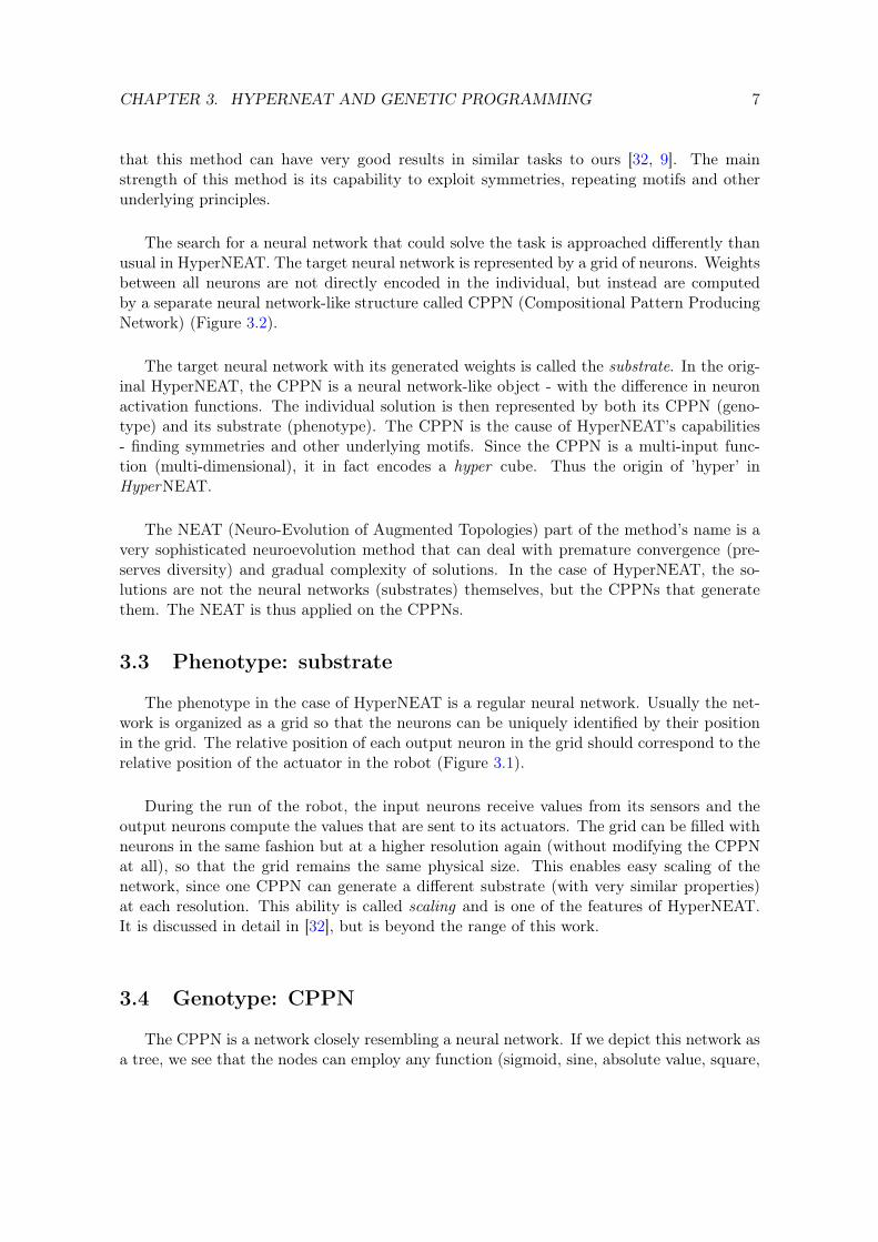
The phenotype in the case of HyperNEAT is a regular neural network. Usually the net-work is organized as a grid so that the neurons can be uniquely identified by their positionin the grid. The relative position of each output neuron in the grid should correspond to therelative position of the actuator in the robot (Figure 3.1).
During the run of the robot, the input neurons receive values from its sensors and theoutput neurons compute the values that are sent to its actuators. The grid can be filled withneurons in the same fashion but at a higher resolution again (without modifying the CPPNat all), so that the grid remains the same physical size. This enables easy scaling of thenetwork, since one CPPN can generate a different substrate (with very similar properties)at each resolution. This ability is called scaling and is one of the features of HyperNEAT.It is discussed in detail in [32], but is beyond the range of this work.
3.4 Genotype: CPPN
The CPPN is a network closely resembling a neural network. If we depict this network asa tree, we see that the nodes can employ any function (sigmoid, sine, absolute value, square,
CHAPTER 3. HYPERNEAT AND GENETIC PROGRAMMING 8
Figure 3.1: Relationship of the substrate and the robot topology
square root etc) and the leaves are input variables into the network. The output node (theroot) just carries the result of the computations coming from inside of the tree.
The input variables, in the case of HyperNEAT, are the coordinates of the chosen neu-rons in the substrate and the output is the synaptic weight value between those neurons.This way, the substrate is constructed by querying its CPPN for weight values between allneurons in the substrate (Figure 3.2). When all the neurons have all the synaptic weightsbetween each other determined, the substrate is ready for use.
The choice of the neuron activation functions enables the CPPN to discover correspond-ing spatial properties in the robot. For instance, absolute value of x can encode Y-axissymmetry, sine of x can encode repeating parts along the robot etc.
The potential of this encoding has been shown in experiments [32, 9] where the CPPN canin fact encode symmetries and other regularities that could hardly be present if direct encod-ing was used. This way, through evolution, the discovered symmetries cause the network torealize that it just copies one leg multiple times into the robot body. This is something thatin previous methods [28, 19, 14] had to be explicitly enforced on the evolution by separatingit into stages [19, 14] or using inner optimization loops [28].
With this approach, the change in the genotype (CPPN) caused by genetic operatorssuch as mutation and crossover does not have to be destructive (like in the case of directencoding), because a change to one table leg is propagated to all other legs (Section 3.1).

CHAPTER 3. HYPERNEAT AND GENETIC PROGRAMMING 9
Figure 3.2: Hypercube encoding example
3.5 Genetic Programming (GP)
Genetic programming (GP) is an evolutionary algorithm-based method for creating com-puter programs [16]. It is a special kind of a evolutionary algorithm, where each individualis represented by a tree of functions and terminals.
The genetic operators commonly used in genetic algorithm methods such as mutationand crossover are also present in GP. The mutation operator takes a random tree node andreplaces it with a newly generated subtree. The crossover (one point crossover), selects anode in each of the two trees coming into the crossover operator and exchanges the subtreesoriginating from those selected points.
The selection in GP is based on the fitness value (measure of the quality of the solution)and can be done through methods like the Roulette wheel, Stochastic Universal Sampling,Tournament Selection or Remainder Stochastic Sampling.
Chapter 4
Robotic simulator Sim
We will use the following robotic simulator for the fitness acquisition and individualrobot behavior visualization. This robotic simulator Sim was created at the Czech TechnicalUniversity by Daniel Fiser and Vojta Vonasek [31]. The Sim combines the physics simulatorOpen Dynamics Engine [24] with the graphics engine OpenSceneGraph [26].
The Sim can be used in both non-visual and visual mode. The non-visual is practicalfor fast robot evaluations during the experiment run and the visual one, obviously, for con-firmation of desired behavior by the experimenter. Usually this confirmation is undertakenafter the experiment is over and the best individual from the evolved population is loadedinto the simulator and shown to the experimenter.
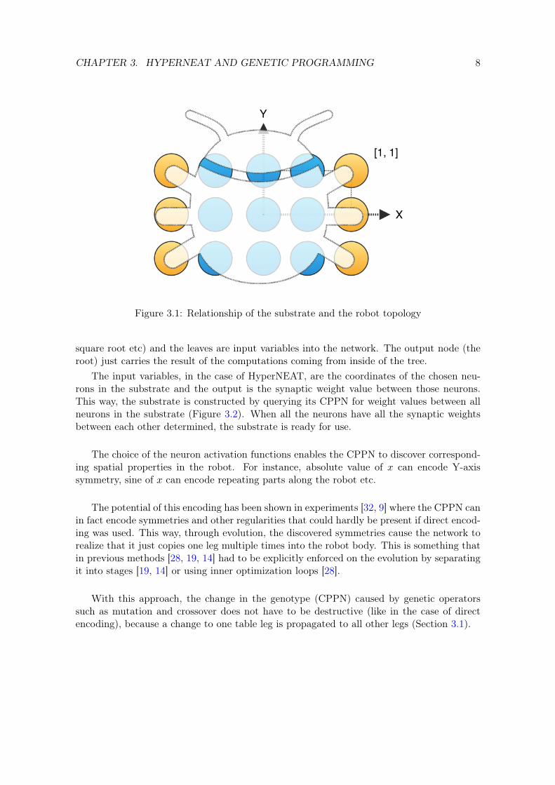
Sim comes with a wide variety of input options, although for our purposes, the SSSAmodular robot input turned out to be the most frictionless approach. SSSA robots are therobots used with the SYMBRION/REPLICATOR projects, thoroughly described and usedin [7]. In our simplified simulator, one SSSA robot consists of a joint connecting the body(cube) and a moving flat connection panel (Figure 4.1). The panel can move in one degreeof freedom around the body in the range of [−π
2 ,π2 ]. What we refer to as a robot in this
work, however, is a set of connected SSSA robots, together forming a structure with manydegrees of freedom (Figure 4.2).
Deeper description of the SSSA robots is not included in this work, because they werejust used as a tool of evaluating the efectivness of the HyperGP algorithm implemented inour framework.
The input of the simulator consists of setting up the simulation parameters (start andstop times, sample time, physics constants) and creating the robot body in the simulator.The creation of the robot body is done through describing the positions and rotations ofeach SSSA body. The simulator then attaches all the bodies that can be attached (are nextto each other). This way we create the robot. Each SSSA body then gets registered to thesimulator for updates.
10

CHAPTER 4. ROBOTIC SIMULATOR SIM 11
Figure 4.1: One SSSA robot
Figure 4.2: Many SSSA pieces forming what we refer to as a robot
Later, during the simulation, an object containing the phenotype outputs for all timesteps is queried for these values. Each of the SSSA bodies queries our object independently.We answer these queries by identifying the source SSSA body by its relative position in thewhole robot and looking up the value (desired rotation angle) which is set as the desired
CHAPTER 4. ROBOTIC SIMULATOR SIM 12
rotation of the SSSA body.
The simulator takes care of moving the SSSA body into the desired rotation over time.It does so by taking the difference between the current and desired rotations and multiplyingit by a gain constant to get the desired angular velocity. The default of the simulator wasgain = −0.5, for our experiments we increased it to gain = −1.0 to get speedier movements.
The position of the center SSSA body is computed at the end of the simulation. Thedifference of the end position and the start position (or position at some delayed time) isconsidered the output of the simulator. We later compute fitness from this translation vector.

Chapter 5
Proposed HyperGP approach
Our approach consists of modifying the HyperNEAT algorithm into HyperGP and addinga bloat control method. Both changes are described in this chapter.
5.1 HyperGP
After researching multiple neuroevolution methods, the HyperNEAT approach seemedbest suited for our task. The ability to encode symmetries and spacial motifs of the robotcould be a great advantage in problems such as robot locomotion. We chose to replace NEATas the evolutionary method with genetic programming (GP), though, for its simplicity andsuggested superiority in certain cases [6]. This change can be seen in Figure 5.1.
Figure 5.1 shows, how our proposed algorithm could be designed with a consideration ofmodularity. The first block on the left symbolizes the process which tweaks the populationin each iteration - in our case GP, in case of HyperNEAT it was the NEAT algorithm. Themiddle block holds the genotype-phenotype mapping used. Even though we are using hyper-encoding in this paper, some kind of direct encoding could also be used for different tasks.The important part is that only the middle block would need to be changed. The blockall the way on the right symbolizes the fitness evaluator. In our case a software simulatoris used, but it could also be a module working in the physical world which would evaluatefitness in real time on real robots and feed the data back to the algorithm.
This exchange of NEAT for GP has been done before in [6]. It requires us to reconsiderthe genotype (CPPN), however. Instead of using a Compositional Pattern Producing Net-work, GP uses functions as genotypes, thus the genotype is called a Compositional PatternProducing Function (CPPF) [6].
The strengths and advantages of indirect encoding for similar tasks have been shownseveral times [32, 9, 6]. With the use of indirect encoding through hyper-encoding and thegenetic programming as the evolutionary method we hope to develop a process that wouldbe able, together with an appropriate robotic simulator, to find some good solutions for the
13

CHAPTER 5. PROPOSED HYPERGP APPROACH 14
Hyper decode SimulatorGPHyperGP:
HyperNEAT: Hyper decode SimulatorNEAT
Figure 5.1: HyperGP derived from HyperNEAT
problem. The process is depicted in Figure 5.2.
5.1.1 Initial population
The process starts with a randomly generated population of small CPPFs (tree-basedfunctions which generate the weights of the neural network). The random initialization canemploy methods such as Full, Grow or Ramped Half-and-Half.
5.1.2 Selection
The selection of individuals that are given a chance to reproduce can be performedthrough Tournament, Roulette or any other selection methods.
5.1.3 Mutation
The selected individuals are mutated with a certain small probability in the followingmatter. A node is chosen in the tree. The subtree originating from that node is removed. Anew, randomly generated subtree is placed onto the node instead.
5.1.4 Recombination
With a certain probability, two selected individuals can recombine in the following matter.A randomly chosen node is found in the first tree. A randomly chosen node is found in thesecond tree. The subtrees, originating from those two points are exchanged between thetrees. Then, both trees are placed into a new population.

CHAPTER 5. PROPOSED HYPERGP APPROACH 15
Fals
e
True
Population N
Selection
Crossover
Mutation
Evaluation
Population N+1Termination conditionFinal population
Initial population
Figure 5.2: GP evolution
5.1.5 Evaluation
The fitness evaluation is performed in two phases. The first phase decodes the CPPF intoits substrate (a neural network controlling the robot). In the second phase, each individualnow possessing both its genotype (CPPF) and phenotype (neural network), is put into thesimulator for fitness computation. The fitness value can be defined as the forward traveleddistance of the simulated robot, the integrated walked path or any other desired behavior.
5.1.6 Termination condition
Since we cannot simulate natural open ended evolution, we need to set a stopping point.The first condition to be satisfied stops the process. One condition is a maximum number oftried generations, another is a goal fitness value, which if any individual in the populationpossesses, causes the evolution to stop.
5.2 Bloat control
A peculiar phenomenon exists in the genetic programming approach. Sometime duringthe evolution, genetic operators might cause individuals to start developing larger trees with-
CHAPTER 5. PROPOSED HYPERGP APPROACH 16
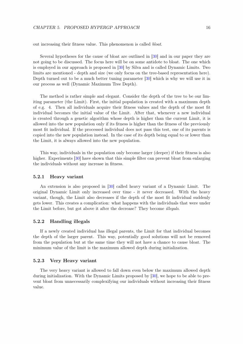
out increasing their fitness value. This phenomenon is called bloat.
Several hypotheses for the cause of bloat are outlined in [30] and in our paper they arenot going to be discussed. The focus here will be on some antidote to bloat. The one whichis employed in our approach is proposed in [30] by Silva and is called Dynamic Limits. Twolimits are mentioned - depth and size (we only focus on the tree-based representation here).Depth turned out to be a much better tuning parameter [30] which is why we will use it inour process as well (Dynamic Maximum Tree Depth).
The method is rather simple and elegant. Consider the depth of the tree to be our lim-iting parameter (the Limit). First, the initial population is created with a maximum depthof e.g. 4. Then all individuals acquire their fitness values and the depth of the most fitindividual becomes the initial value of the Limit. After that, whenever a new individualis created through a genetic algorithm whose depth is higher than the current Limit, it isallowed into the new population only if its fitness is higher than the fitness of the previouslymost fit individual. If the processed individual does not pass this test, one of its parents iscopied into the new population instead. In the case of its depth being equal to or lower thanthe Limit, it is always allowed into the new population.
This way, individuals in the population only become larger (deeper) if their fitness is alsohigher. Experiments [30] have shown that this simple filter can prevent bloat from enlargingthe individuals without any increase in fitness.
5.2.1 Heavy variant
An extension is also proposed in [30] called heavy variant of a Dynamic Limit. Theoriginal Dynamic Limit only increased over time - it never decreased. With the heavyvariant, though, the Limit also decreases if the depth of the most fit individual suddenlygets lower. This creates a complication: what happens with the individuals that were underthe Limit before, but got above it after the decrease? They become illegals.
5.2.2 Handling illegals
If a newly created individual has illegal parents, the Limit for that individual becomesthe depth of the larger parent. This way, potentially good solutions will not be removedfrom the population but at the same time they will not have a chance to cause bloat. Theminimum value of the limit is the maximum allowed depth during initialization.
5.2.3 Very Heavy variant
The very heavy variant is allowed to fall down even below the maximum allowed depthduring initialization. With the Dynamic Limits proposed by [30], we hope to be able to pre-vent bloat from unnecessarily complexifying our individuals without increasing their fitnessvalue.

Chapter 6
Implementation
In order to verify the efficiency of the proposed solutions, the whole algorithm needed tobe implemented as a computer program. The focus was mainly on:
• maximizing computational speed
• high expandability of the program in the future
• automatic support of multi-core processors
• low memory requirements
• at least some platform independence
These objectives fundamentally affected the choice of the programming language, plat-form and software design.
6.1 Programming environment
6.1.1 Programming language
Due to the need of both low level and object-oriented features, C++ was chosen as theprogramming language that could satisfy all the mentioned goals. There were other candi-date languages, but C++ was the best choice for the following reasons.
The other obvious choice would be Java, as the world’s most popular application pro-gramming language [29]. Although, some sources claim that C++ should be faster thanJava by principle (Java runs on a virtual machine) [13]. Certain benchmarks find it difficultto compare languages, since each is better at a different task [8]. Also, Java is much moreplatform independent than C++. However, we did not choose Java for its lack of user mem-ory control (Java uses runtime garbage collection) in addition to the speed disadvantages.
Another option was Objective-C, a C-based, objective-oriented language in developmentby Apple, Inc. The platform dependence on the Darwin architecture (poor support on Linuxmachines) made us not really consider it, even though the choice of the compiler later lockedus down for the near future.
17

CHAPTER 6. IMPLEMENTATION 18
6.1.2 Compiler
Due to the fact that most of the implementation took place on a MacBook Pro, runningOS X 10.8 and Xcode as the development environment, we chose the Clang/LLVM compiler[20] instead of the more common GCC compiler. Some sources claim that Clang/LLVM isfaster in compilation, more efficient and produces better binaries of C++ code [17].
Clang/LLVM even uses its own implementation of the C++ standard library (libc++).Unfortunately, tested release versions are only available for the Darwin architecture meaningthat compiling at Linux machines would be unreliable at this time (the libc++ library forLinux machines is in the experimental stage at the moment) [21].
Trying to make the code future-proof, we wanted to use the latest C++11 languagestandard. Clang/LLVM was build to be feature-complete and designed for C++11 from thebeginning [20].
6.1.3 Platform
Programming on Apple’s platform, there were many advantages in using the native com-piler with C++. The main one is the support of Grand Central Dispatch (GCD), a multi-thread multi-core management system, available for the C++ language [4].
The advantage of using GCD instead of hard-coding POSIX threads is that only indi-vidual blocks of code are submitted to GCD for asynchronous processing. GCD takes careof creating and destroying threads and is able to use all available processor cores. Thiseliminates the need to know the number of available cores on the target machine. GCD justuses them all without the programmer having to program anything extra [4].
All these features are in development for the Linux platform, as well. However, at thetime of this writing, most of them are still in experimental stage and are not recommendedto be used for serious work.
The choice of IDE (Integrated Development Environment) was easy. Having workedwith Xcode (by Apple, Inc.) [5] for almost two years and knowing that Xcode was built forObjective-C and C++ development, no other IDE was considered. Shell and Python scriptcoding was done in Sublime Text 2 [3] and MATLAB scripts in the MATLAB app [23].
6.2 The cic framework
In order to successfully test the proposed form of HyperGP algorithm, a solid implemen-tation had to be proposed. Keeping the future modifications in mind, a framework namedcic was developed. Since we might want to test different algorithms than GP or use differentencoding than the hypercube-based, generic interfaces and types had to be defined in advance.

CHAPTER 6. IMPLEMENTATION 19
The best way of to present any population-based algorithm is, for our purpose, to look atthe population as one object and the algorithm as a block modifying that object. Also,we needed a way to work with the particular individuals, as the items contained by thepopulation.
Starting with the most abstract interfaces, these main three types of objects were defined
• Individual
• Population
• Population Modifier
All the particular types brought in with particular algorithms and processes have to in-herit from either of these three types. That is how cic was designed. Figure 6.1 shows howtwo particular algorithms use this sort of design to define all needed types.
Figure 6.1: cic types hierarchy with symreg and hyperGP
As it was mentioned, the actual implementation of the cic framework did not targetonly one genetic algorithm-based experiment. Since the HyperGP experiment itself was nottrivial to program and test, another simpler experiment was used as a proof-of-concept forthe framework to help debug it before HyperGP would run in it.
A generic symbolic regression experiment was used first. The biggest advantage of thisapproach was that about a half of the codebase was shared between symbolic regression andHyperGP.

CHAPTER 6. IMPLEMENTATION 20
6.2.1 Experiment: Symbolic Regression - cic::genetic::symreg
The goal of symbolic regression is finding a function that best satisfies certain constraints.Genetic, population-based approach was used here in the following matter (also depicted inFigure 6.2):
Figure 6.2: symreg workings in cic
In our case first a function was selected and n equidistant points were chosen in a rangermin, rmax. These worked as a reference set of points for the simulator. Each evaluatedfunction was sampled in the same matter and the sum of absolute differences between it andthe reference of all points was computed. The negative value of that sum was used as thefitness value (since we used the higher-fitness-is-better approach).
If x is a vector of points computed by a tested function and r is the vector of pointsgenerated by our reference function, then fitness of the i-th individual fi was computed as
ei =M∑k=1
|xk − rk| (6.1)
fi = −ei (6.2)
where fi is the fitness of the i-th individual.
The symreg implementation of the symbolic regression experiment was very helpful withdebugging of the framework. The framework ran only symreg for a couple of weeks during the
CHAPTER 6. IMPLEMENTATION 21
development and still works as a benchmark experiment. During that time, support for mul-tithreaded computing was added (with the use of GCD, Section 6.1.3), MATLAB interfacewas developed (Section 6.4.2) and XML serializer/parser was implemented (Section 6.4.1).
6.2.2 Experiment: HyperGP - cic::genetic::hyperGP
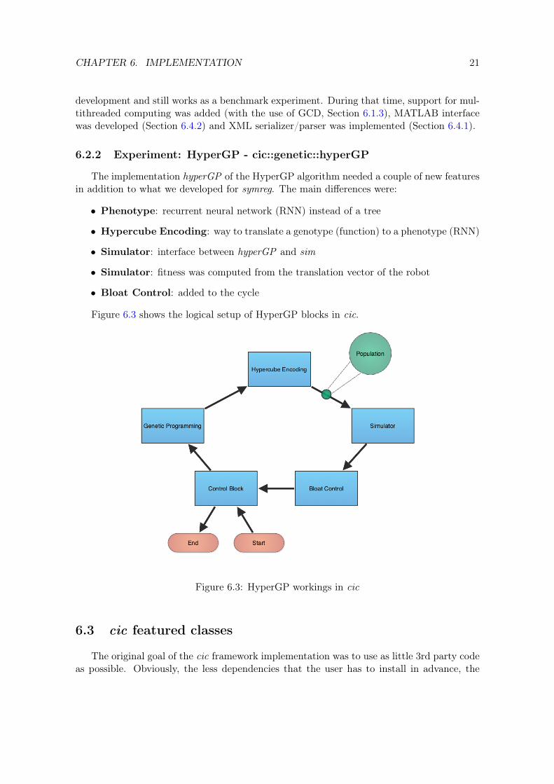
The implementation hyperGP of the HyperGP algorithm needed a couple of new featuresin addition to what we developed for symreg. The main differences were:
• Phenotype: recurrent neural network (RNN) instead of a tree
• Hypercube Encoding: way to translate a genotype (function) to a phenotype (RNN)
• Simulator: interface between hyperGP and sim
• Simulator: fitness was computed from the translation vector of the robot
• Bloat Control: added to the cycle
Figure 6.3 shows the logical setup of HyperGP blocks in cic.
Figure 6.3: HyperGP workings in cic
6.3 cic featured classes
The original goal of the cic framework implementation was to use as little 3rd party codeas possible. Obviously, the less dependencies that the user has to install in advance, the

CHAPTER 6. IMPLEMENTATION 22
better. In the end, several common libraries (Section 6.4) were used for certain purposes,but the actual working of the algorithm does not depend on any of them (the libraries aremainly used as I/O tools).
The implementation of the core pieces is discussed in the rest of this chapter.
6.3.1 cic::genetic::Individual
Since all the algorithmic work is achieved by population modifiers, in cic the Individualclass only works as data storage of the particular gene. The genotype, phenotype, fitnessvalue are stored directly in the Individual (Figure 6.4). Optionally, the experiment can useIndividual’s pointer to its parent - which is taken care of by genetic operators. One morekey-value storage is contained in every Individual. Population modifiers can use that storageto assign attributes to the Individual (e.g. Bloat Control needs to mark Individuals illegalin certain cases).
Figure 6.4: cic::Individual
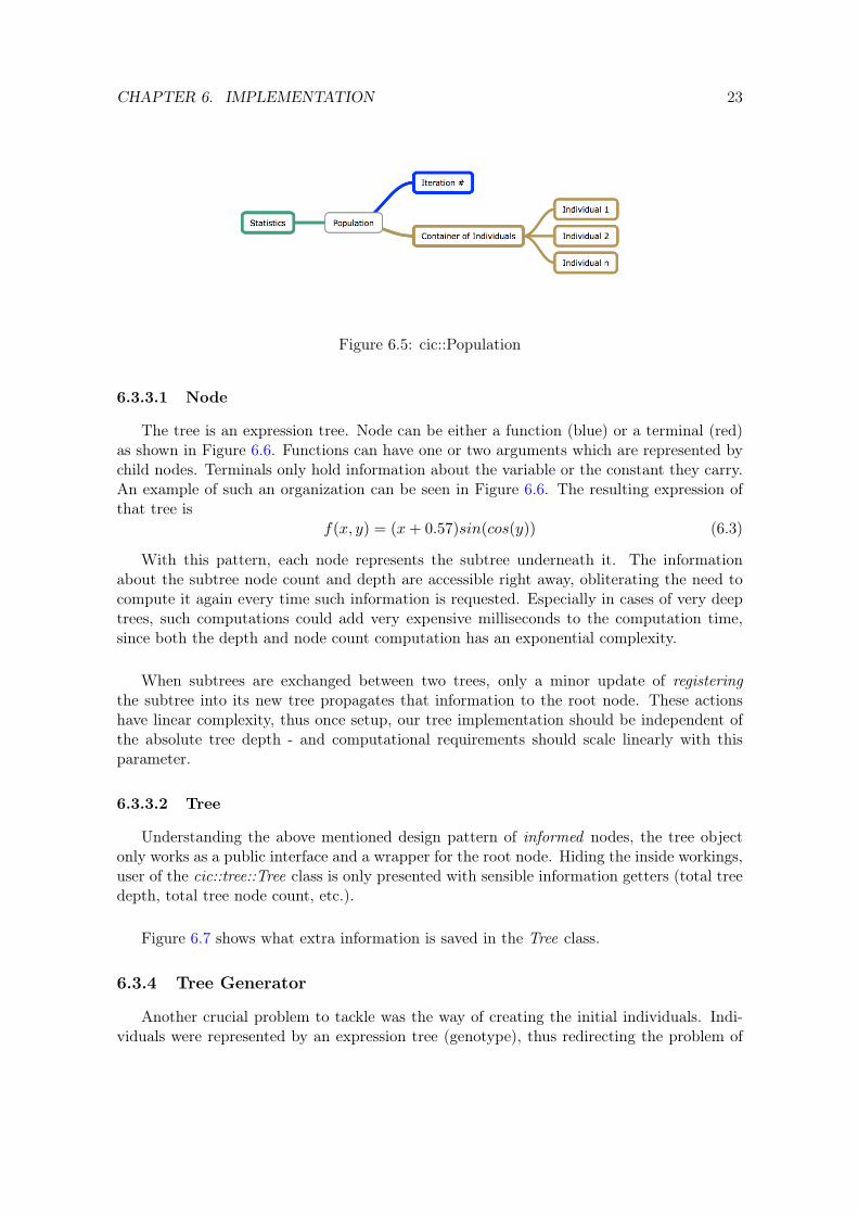
6.3.2 cic::genetic::Population
The Population class is a container of Individuals. Support of iterators has been addedfor easier enumeration of Individuals. An integer marking the Population’s iteration numberworks as its identifier (Figure 6.5). Individuals are stored by making a copy of their sharedpointer. This way, when the last owner deletes the pointer, the Individual gets deleted frommemory automatically. A copy of the Population is exported to a XML file during and at theend of each experiment and can be again loaded as the starting point for a new experiment.
6.3.3 cic::tree::Tree
The genotype in the HyperGP experiment was a multidimensional (hypercubic) function.Functions can be easily digitally represented in the form of a binary tree. In order to in-crease the speed of the tree result computation, decision was made to save more informationinto the tree nodes at the cost of memory consumption. A proprietary implementation wasneeded and one was proposed and implemented.
CHAPTER 6. IMPLEMENTATION 23
Figure 6.5: cic::Population
6.3.3.1 Node
The tree is an expression tree. Node can be either a function (blue) or a terminal (red)as shown in Figure 6.6. Functions can have one or two arguments which are represented bychild nodes. Terminals only hold information about the variable or the constant they carry.An example of such an organization can be seen in Figure 6.6. The resulting expression ofthat tree is
f(x, y) = (x+ 0.57)sin(cos(y)) (6.3)
With this pattern, each node represents the subtree underneath it. The informationabout the subtree node count and depth are accessible right away, obliterating the need tocompute it again every time such information is requested. Especially in cases of very deeptrees, such computations could add very expensive milliseconds to the computation time,since both the depth and node count computation has an exponential complexity.
When subtrees are exchanged between two trees, only a minor update of registeringthe subtree into its new tree propagates that information to the root node. These actionshave linear complexity, thus once setup, our tree implementation should be independent ofthe absolute tree depth - and computational requirements should scale linearly with thisparameter.
6.3.3.2 Tree
Understanding the above mentioned design pattern of informed nodes, the tree objectonly works as a public interface and a wrapper for the root node. Hiding the inside workings,user of the cic::tree::Tree class is only presented with sensible information getters (total treedepth, total tree node count, etc.).
Figure 6.7 shows what extra information is saved in the Tree class.
6.3.4 Tree Generator
Another crucial problem to tackle was the way of creating the initial individuals. Indi-viduals were represented by an expression tree (genotype), thus redirecting the problem of

CHAPTER 6. IMPLEMENTATION 24
Figure 6.6: Example nodes connected into a tree
Figure 6.7: Tree types hierarchy
individual generation to tree generation. The random tree generation is important in severalparts of the experiment:
• initial trees of the initial population
• subtree generation for the mutation operator
• creation of new individuals after some get removed from the population (e.g. bloatcontrol)
There are several known and used methods, which are fairly simple, such as Grow, Fulland Ramped Half-and-Half [16]. In addition, another one, called PTC1 [22] was imple-mented to be able to control the generated trees’ parameters more precisely.
CHAPTER 6. IMPLEMENTATION 25
For the scope of the following methods, A is the set of all available nodes, T the set ofall available terminal nodes and F the set of all the function nodes. The maximum depth isdenoted dmax.
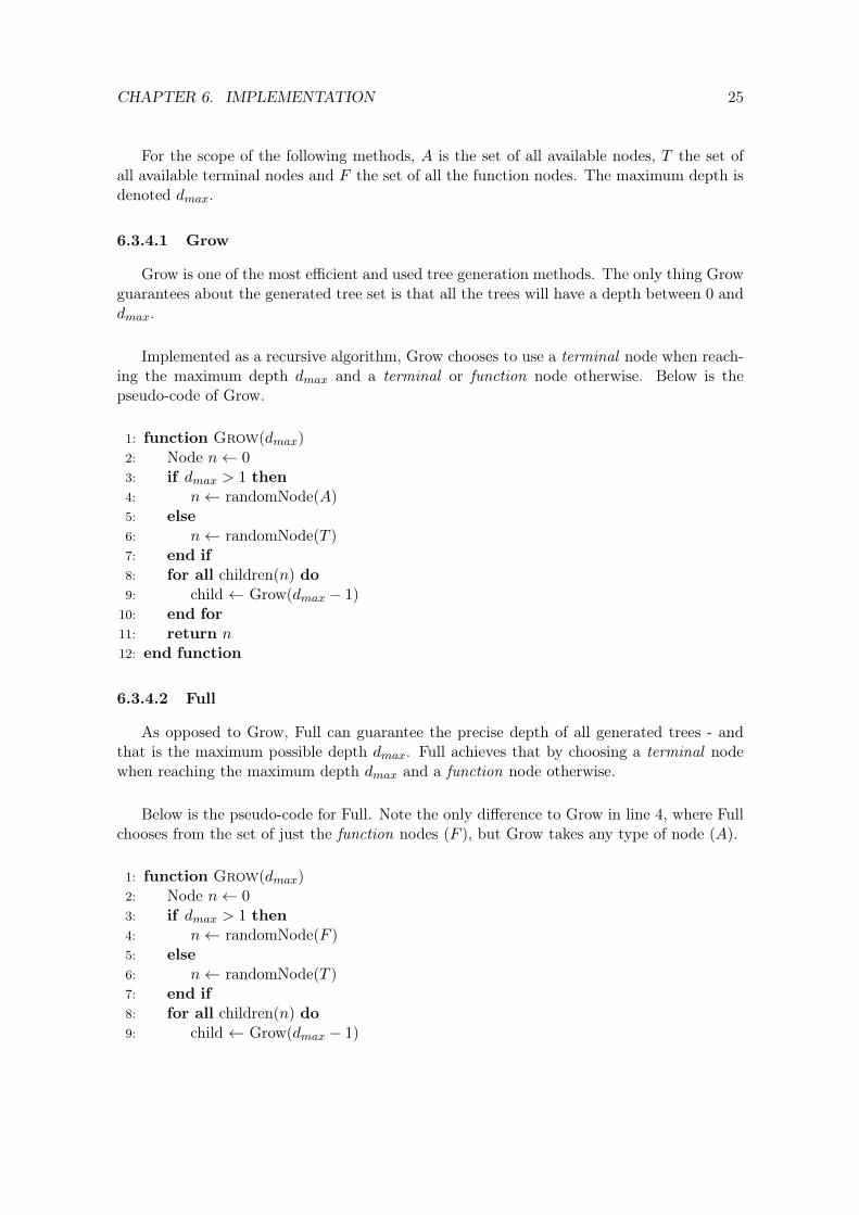
6.3.4.1 Grow
Grow is one of the most efficient and used tree generation methods. The only thing Growguarantees about the generated tree set is that all the trees will have a depth between 0 anddmax.
Implemented as a recursive algorithm, Grow chooses to use a terminal node when reach-ing the maximum depth dmax and a terminal or function node otherwise. Below is thepseudo-code of Grow.
1: function Grow(dmax)2: Node n← 03: if dmax > 1 then4: n← randomNode(A)5: else6: n← randomNode(T )7: end if8: for all children(n) do9: child ← Grow(dmax − 1)
10: end for11: return n12: end function
6.3.4.2 Full
As opposed to Grow, Full can guarantee the precise depth of all generated trees - andthat is the maximum possible depth dmax. Full achieves that by choosing a terminal nodewhen reaching the maximum depth dmax and a function node otherwise.
Below is the pseudo-code for Full. Note the only difference to Grow in line 4, where Fullchooses from the set of just the function nodes (F ), but Grow takes any type of node (A).
1: function Grow(dmax)2: Node n← 03: if dmax > 1 then4: n← randomNode(F )5: else6: n← randomNode(T )7: end if8: for all children(n) do9: child ← Grow(dmax − 1)
CHAPTER 6. IMPLEMENTATION 26
10: end for11: return n12: end function
6.3.4.3 Ramped Half-and-Half
Grow is great for creating a population diverse in depth, whereas Full guarantees thatall trees will be as full as possible. However, neither of these methods works perfectly forall applications, which is why a combination of these two, called Ramped Half-and-Half hasbeen the most preferable. It uses Grow and Full as described above in the following matter:half of the population is created with Grow; the other half is created by applying Full with asmall maximum depth (0, 1, 2 or any other) gradually ramping up to dmax. Equal number (ifpossible) of the half population devoted to Full gets created with different maximum depthsapplied to Full.
This particular method enables the population to be diverse both in depth and in usednodes. Ramped Half-and-Half’s ratio of effectiveness to simplicity makes it a great candidatefor our application.
6.3.4.4 PTC1
Trying to expand the theoretical boundaries of our tree generator, one more generationmethod was implemented. Described in [22], PTC1 (Probabilistic Tree-Creation) providesmuch more control over the generated tree set. Being able to guarantee the average tree size,maximum depth and even the occurrence probability of each node provides us with muchmore power.
The gist of PTC1 is that it is a modified version of the Grow generation method, men-tioned above. The input data to PTC1 is
• expected (average) tree size Etree
• arity bf for each function node f ∈ F
• probability qf for each function node f ∈ F
• probability qt for each terminal node t ∈ T
• maximum depth dmax
The algorithm first computes p, the probability of choosing a function node. This prob-ability is constant for the whole run, so it needs to be computed only once before the startof the generation.
p =1− 1
Etree∑f∈F
qfbn(6.4)
Once p is computed, the tree generation runs as follows

CHAPTER 6. IMPLEMENTATION 27
1: Tree ← PTC1(0)2: function PTC1(d)3: if d == dmax then4: return terminal from T (by qt probabilities)5: else6: if chose f from A with probability p then7: choose f ∈ F (by qf probabilities)8: for all arguments of f do argument ← PTC1(d+ 1)9: end for
10: return f11: else12: return terminal from T (by qt probabilities)13: end if14: end if15: end function
6.3.5 cic::nn::Network
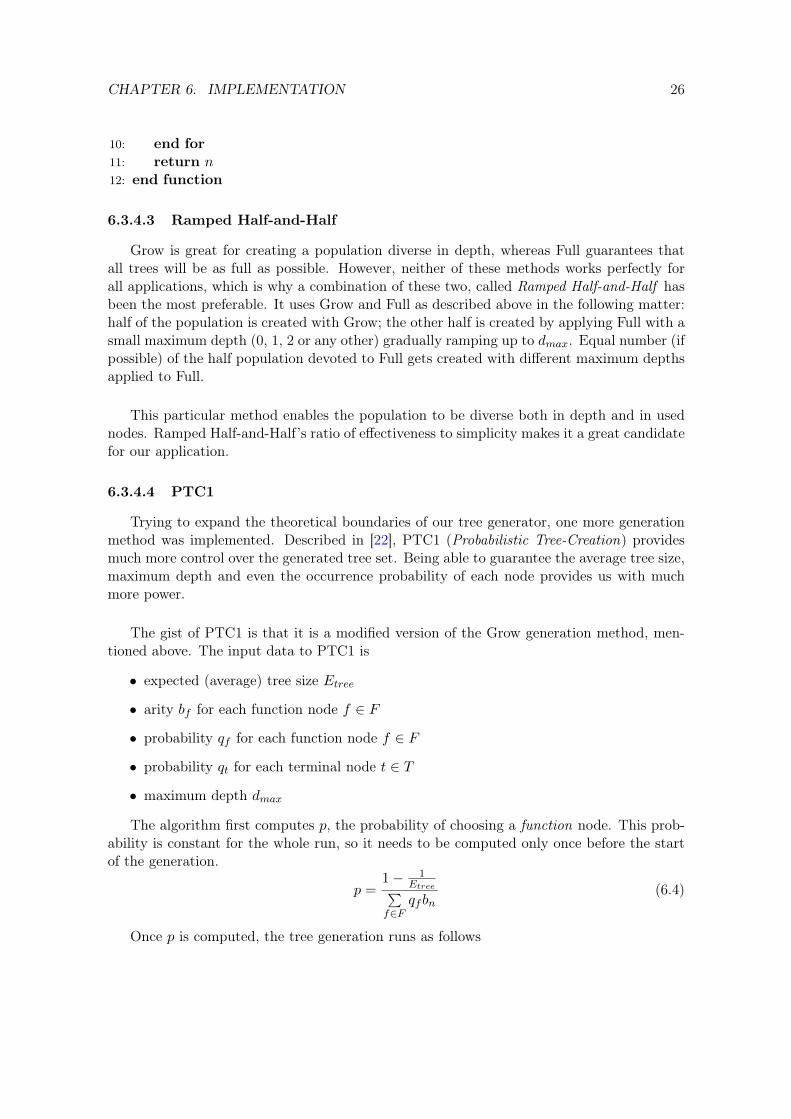
In the HyperGP algorithm, the phenotype of each individual is a neural network. Thisneural network is the manifestation of the genotype (function), since the synaptic weightsbetween neurons are computed by the genotype’s function. The problem faced with a regularneural network is the lack of memory-like behavior. In the HyperGP simulator, a conceptof time needs to be present in the genotype. To solve this issue, a recurrent neural networkwas used. Recurrent types can simulate discrete time systems through synapses not onlygoing from input to hidden (1) layer and hidden to output (2), but also hidden to hidden(3), output to output (4) and even output to hidden (5). And all synapses not going in theforward direction (types 3, 4, 5) need to be evaluated with one time step delay (Figure 6.8).
In other words, the network will hold internal values from the past and take them intoaccount when computing the future outputs. This is exactly what is needed to avoid bringingtime as an extra input into the network. In our particular implementation, every neuronsaves into memory its output value and the current time. When the network outputs arebeing computed and this information is queried, the neuron looks into its memory first andthen if it does not find the value for the current time, just computes it and saves it again.This way, we - once again - sacrifice a piece of memory for faster evaluation.
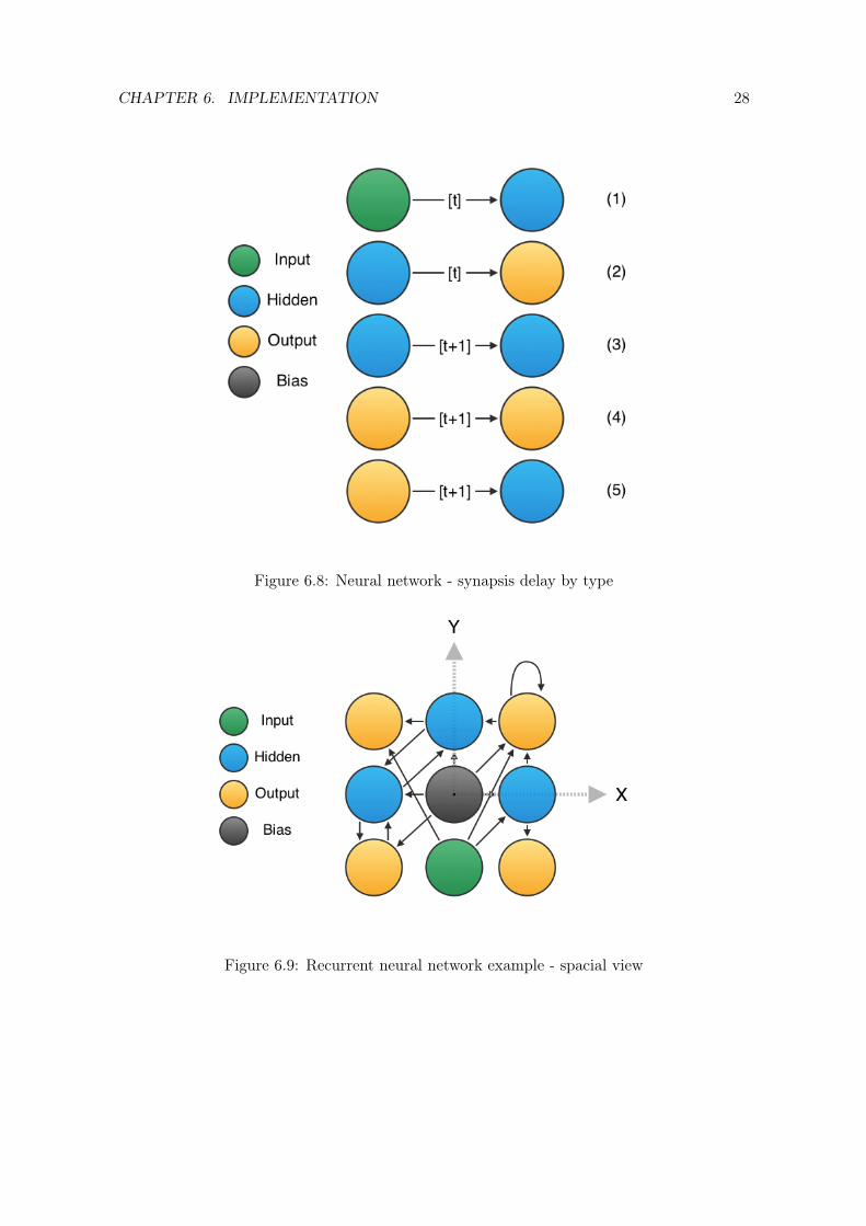
The spatial setup of the network needs to conform to the robot spatial architecture (asexplained in Section 3.3). An example of such a network can be seen in Figure 6.9. Onthe other hand, neural networks are generally approached from a layer-focused point of view(Figure 6.10). The layer approach also makes clearer why some synapses transfer signalimmediately (forward going) and some need to be one time step delayed (all other).
CHAPTER 6. IMPLEMENTATION 28
Figure 6.8: Neural network - synapsis delay by type
Figure 6.9: Recurrent neural network example - spacial view

CHAPTER 6. IMPLEMENTATION 29
Figure 6.10: Recurrent neural network example - layer view
6.4 Tools and libraries
There was no need to re-implement certain tools for our needs, such as the roboticsimulator and a simple plotting tool. Several common libraries and tools were used for thosepurposes.
6.4.1 libxml2
Any computations that take place in the cic program are immediately lost with the ter-mination of the program. That is the reason why a decent way of saving results, individualsand settings to a permanent storage was needed. One of the most popular choices was XML(Extensible Markup Language) [33, 25]. The great advantage of saving data to XML, insteadof a binary file, for example, is that it is human readable. This way, even after the XMLhas been exported from the program to the hard drive, we can read and modify the file byhand. These modifications do not corrupt the file content, meaning it can be again loadedinto the program and used as a starting point for further experiments.
In the search for a simple XML C++ parser library the winner ended up being libxml2,because it is very simple, robust and already present on every Mac (thus eliminating theneed to install extra software) [35].
6.4.2 MATLAB
Average and maximum fitness, tree depth, size etc. are all the properties developed dur-ing the runtime of the experiment and all this data is most helpful when seen in a plot of

CHAPTER 6. IMPLEMENTATION 30
some sort. The MATLAB libraries, distributed with every copy of the MATLAB app seemedappropriate for several reasons. For one, once the data is out of the experiment and in aMATLAB file, further analysis can take place independently on the actual experiment. Foranother, MATLAB libraries provide a simple way of opening and using a MATLAB instanceon the background, invoked and controller from C++ code.
The MATLAB integration in cic is very crude at its current state. All data is onlycopied into a MATLAB instance, saved to a .mat file and optionally plotted right awayfor the experimenter to see. Some simple inter-experiment data analysis is done by extraMALTAB scripts that are distributed with the cic codebase.
6.4.3 Sim
The intention from the start was to use the robotic simulator developed by D. Fiser andV. Vonasek at FEE, CTU in Prague for the SYMBRION/REPLICATOR projects [31]. Themain advantages over the other Robot 3D simulator are [2]
• lightweight
• can perform faster-than-real-time simulations
• supports running of several instances in several threads
The simulator setup consists of subclassing the Sim class and setting up the simulationworld parameters, creating the arena and creating the actual robot. Then another object isassigned as the controller of the robot and the simulator queries the controller for updatesof the desired rotations of the robot legs regularly. In the case of HyperGP, a Neural Con-troller was created to take care of translating the outputs of the neural network (substrate- mentioned in Section 3.3) into desired rotation angles of the robot joints.
6.4.4 Other tools
Other software tools were crucial during the implementation phase. One was the packagemanager for Mac called homebrew [12]. Homebrew was very useful during installation oflibraries and tools. Also, other than C++, Python was also used for automation of filesorting (each experiment output 6 files and we ran hundreds of experiments).
Chapter 7
Testing
Rigorous experiments are crucial to every algorithm development. In order to either con-firm or dismiss the efficiency of the HyperGP algorithm, we needed to prepare tests whichwould cover as much parameter space as possible and inform us about HyperGP’s strengthsand weaknesses.
Fortunately, as part of the cic framework, a powerful experiment I/O and result record-ing was implemented. This way, after each test run was over, the framework exported thedata in the xml format (settings, population with all individuals) and the statistics in themat format. This way, we wrote scripts to account for any number of repeating experimentsand statistically process the data in a matter of seconds.
This chapter first describes the setup of the experiments, the types of robots used and allthe different tested parameters. Then it proceeds to the experimental data recorded duringour testing phase.
Rendered videos of selected developed robots are present on the disclosed disk as well ason the website of this project [11].
7.1 Experimental setup
7.1.1 Tested robot topologies
For the proof-of-concept testing, we created three types of robots. The goal was to testseveral robot types, the way they are assembled, whether extra legs affect fitness and so on.The types are
• Robot R0, 5 x 5 cubes, x-axis movement, Figure 4.2
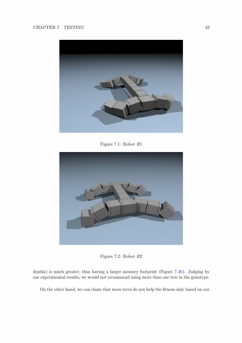
• Type R1, 7 x 7 cubes, y-axis movement, Figure 7.1
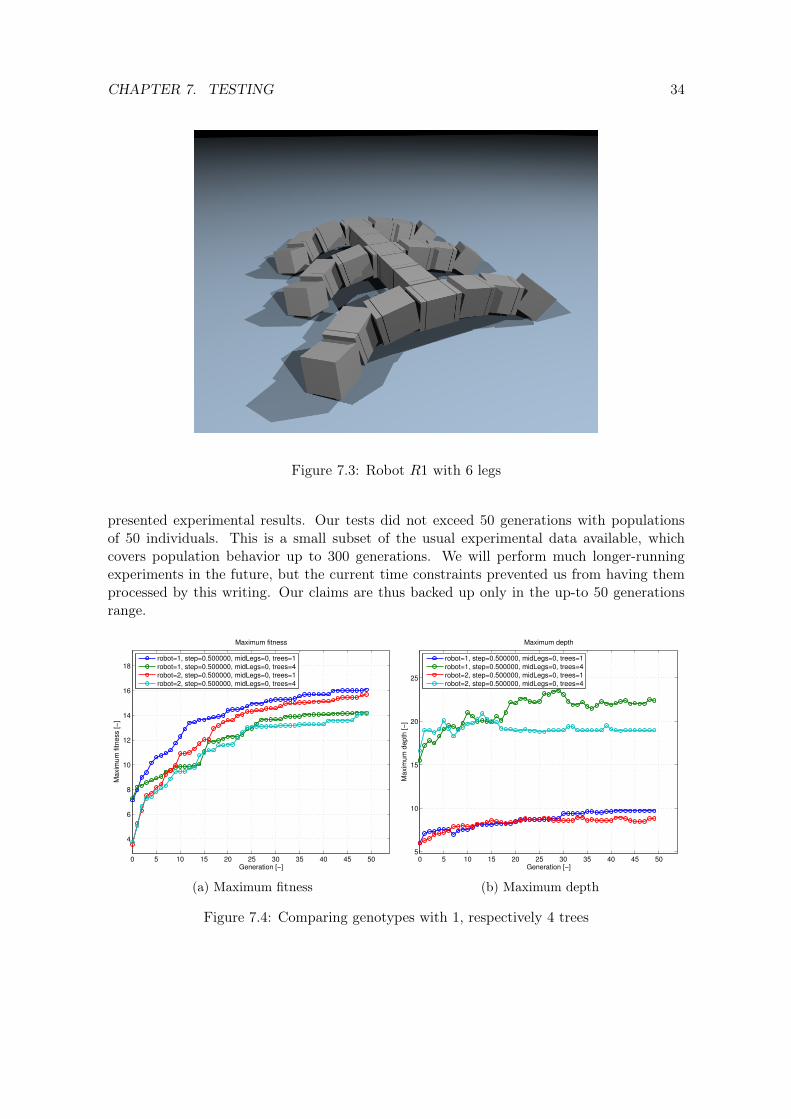
• Type R2, 7 x 5 cubes, y-axis movement, Figure 7.2
31
CHAPTER 7. TESTING 32
7.1.2 Fitness
The search for the perfect fitness function for each robot was not trivial. We tried expo-nential functions dependent on the distance traveled, mentioned in [9] and very sophisticatedmeasures like this. However, the added complexity did not bring any improvements, so weused a very simple equation instead.
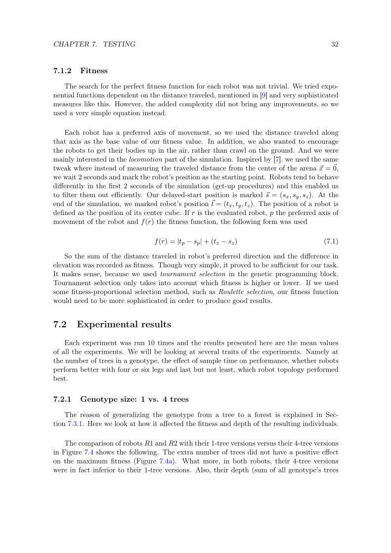
Each robot has a preferred axis of movement, so we used the distance traveled alongthat axis as the base value of our fitness value. In addition, we also wanted to encouragethe robots to get their bodies up in the air, rather than crawl on the ground. And we weremainly interested in the locomotion part of the simulation. Inspired by [7], we used the sametweak where instead of measuring the traveled distance from the center of the arena ~x = ~0,we wait 2 seconds and mark the robot’s position as the starting point. Robots tend to behavedifferently in the first 2 seconds of the simulation (get-up procedures) and this enabled usto filter them out efficiently. Our delayed-start position is marked ~s = (sx, sy, sz). At theend of the simulation, we marked robot’s position ~t = (tx, ty, tz). The position of a robot isdefined as the position of its center cube. If r is the evaluated robot, p the preferred axis ofmovement of the robot and f(r) the fitness function, the following form was used
f(r) = |tp − sp|+ (tz − sz) (7.1)
So the sum of the distance traveled in robot’s preferred direction and the difference inelevation was recorded as fitness. Though very simple, it proved to be sufficient for our task.It makes sense, because we used tournament selection in the genetic programming block.Tournament selection only takes into account which fitness is higher or lower. If we usedsome fitness-proportional selection method, such as Roulette selection, our fitness functionwould need to be more sophisticated in order to produce good results.
7.2 Experimental results
Each experiment was run 10 times and the results presented here are the mean valuesof all the experiments. We will be looking at several traits of the experiments. Namely atthe number of trees in a genotype, the effect of sample time on performance, whether robotsperform better with four or six legs and last but not least, which robot topology performedbest.
7.2.1 Genotype size: 1 vs. 4 trees
The reason of generalizing the genotype from a tree to a forest is explained in Sec-tion 7.3.1. Here we look at how it affected the fitness and depth of the resulting individuals.
The comparison of robots R1 and R2 with their 1-tree versions versus their 4-tree versionsin Figure 7.4 shows the following. The extra number of trees did not have a positive effecton the maximum fitness (Figure 7.4a). What more, in both robots, their 4-tree versionswere in fact inferior to their 1-tree versions. Also, their depth (sum of all genotype’s trees
CHAPTER 7. TESTING 33
Figure 7.1: Robot R1
Figure 7.2: Robot R2
depths) is much greater, thus having a larger memory footprint (Figure 7.4b). Judging byour experimental results, we would not recommend using more than one tree in the genotype.
On the other hand, we can claim that more trees do not help the fitness only based on our
CHAPTER 7. TESTING 34
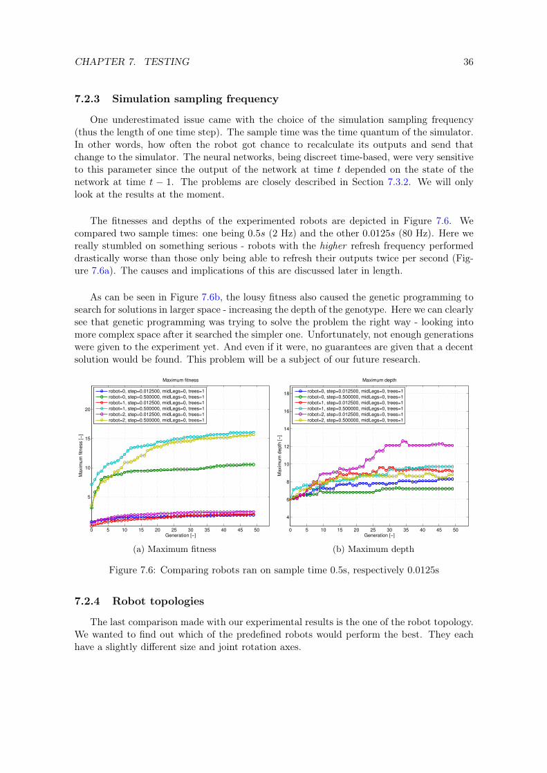
Figure 7.3: Robot R1 with 6 legs
presented experimental results. Our tests did not exceed 50 generations with populationsof 50 individuals. This is a small subset of the usual experimental data available, whichcovers population behavior up to 300 generations. We will perform much longer-runningexperiments in the future, but the current time constraints prevented us from having themprocessed by this writing. Our claims are thus backed up only in the up-to 50 generationsrange.
0 5 10 15 20 25 30 35 40 45 50
4
6
8
10
12
14
16
18
Maximum fitness
Generation [−]
Maxim
um
fitness [−
]
robot=1, step=0.500000, midLegs=0, trees=1
robot=1, step=0.500000, midLegs=0, trees=4
robot=2, step=0.500000, midLegs=0, trees=1
robot=2, step=0.500000, midLegs=0, trees=4
(a) Maximum fitness
0 5 10 15 20 25 30 35 40 45 505
10
15
20
25
Maximum depth
Generation [−]
Maxim
um
depth
[−
]
robot=1, step=0.500000, midLegs=0, trees=1
robot=1, step=0.500000, midLegs=0, trees=4
robot=2, step=0.500000, midLegs=0, trees=1
robot=2, step=0.500000, midLegs=0, trees=4
(b) Maximum depth
Figure 7.4: Comparing genotypes with 1, respectively 4 trees

CHAPTER 7. TESTING 35
7.2.2 Number of legs: 4 vs. 6
Another probed parameter of the robots was the number of used legs. The robots R1 andR2 had their torso long enough that they could receive an extra pair of legs in the middle.An example is the robot R1 depicted with only 4 legs in Figure 7.1, but with the extra pair,having a total of 6 legs in Figure 7.3.
The gist was that the extra pair of legs might work as an assistant pair for the front andrear pairs. The 6-legged robots could theoretically develop a more complex motion patternand solve the locomotion problem more efficiently.
The results can be seen in Figure 7.5 (midLegs = 0 marks robots with 4 legs, midLegs =1 marks robots with 6 legs). It seems that up to the 15th generation, both the R1 and R2developed better with the extra pair of legs (Figure 7.4a). However, by the 20th generation,the 4-leg versions caught up to them and from then on, the fitness was very similar. Thusthe extra pair of legs really did help the robot, especially in the beginning phase of roughlydeveloped individuals.
When looking at the maximum depth parameter in Figure 7.4b, we see that the robotR1 was forced to develop significantly larger trees in the 4-leg version. This fact correspondswith the fitness, meaning that the lower the fitness, the larger trees are explored by geneticprogramming (with the help of bloat control, forcing the trees to grow gradually rather thanrandomly). Robot R2 had very similar results for both 4 and 6-leg versions. This might becaused by R2’s torso being only 5 cubes long as opposed to R1 that has 7 cubes across. Theleg pairs are much closer in R1, enabling more frequent collisions between them - strippingthe robot of its advantage. This would explain the similarity between the fitness of the twoversions.
0 5 10 15 20 25 30 35 40 45 50
4
6
8
10
12
14
16
18
Maximum fitness
Generation [−]
Maxim
um
fitness [−
]
robot=1, step=0.500000, midLegs=0, trees=1
robot=1, step=0.500000, midLegs=1, trees=1
robot=2, step=0.500000, midLegs=0, trees=1
robot=2, step=0.500000, midLegs=1, trees=1
(a) Maximum fitness
0 5 10 15 20 25 30 35 40 45 50
5
6
7
8
9
10
11
Maximum depth
Generation [−]
Maxim
um
depth
[−
]
robot=1, step=0.500000, midLegs=0, trees=1
robot=1, step=0.500000, midLegs=1, trees=1
robot=2, step=0.500000, midLegs=0, trees=1
robot=2, step=0.500000, midLegs=1, trees=1
(b) Maximum depth
Figure 7.5: Comparing robots with 4, respectively 6 legs
CHAPTER 7. TESTING 36
7.2.3 Simulation sampling frequency
One underestimated issue came with the choice of the simulation sampling frequency(thus the length of one time step). The sample time was the time quantum of the simulator.In other words, how often the robot got chance to recalculate its outputs and send thatchange to the simulator. The neural networks, being discreet time-based, were very sensitiveto this parameter since the output of the network at time t depended on the state of thenetwork at time t − 1. The problems are closely described in Section 7.3.2. We will onlylook at the results at the moment.
The fitnesses and depths of the experimented robots are depicted in Figure 7.6. Wecompared two sample times: one being 0.5s (2 Hz) and the other 0.0125s (80 Hz). Here wereally stumbled on something serious - robots with the higher refresh frequency performeddrastically worse than those only being able to refresh their outputs twice per second (Fig-ure 7.6a). The causes and implications of this are discussed later in length.
As can be seen in Figure 7.6b, the lousy fitness also caused the genetic programming tosearch for solutions in larger space - increasing the depth of the genotype. Here we can clearlysee that genetic programming was trying to solve the problem the right way - looking intomore complex space after it searched the simpler one. Unfortunately, not enough generationswere given to the experiment yet. And even if it were, no guarantees are given that a decentsolution would be found. This problem will be a subject of our future research.
0 5 10 15 20 25 30 35 40 45 50
5
10
15
20
Maximum fitness
Generation [−]
Maxim
um
fitness [−
]
robot=0, step=0.012500, midLegs=0, trees=1
robot=0, step=0.500000, midLegs=0, trees=1
robot=1, step=0.012500, midLegs=0, trees=1
robot=1, step=0.500000, midLegs=0, trees=1
robot=2, step=0.012500, midLegs=0, trees=1
robot=2, step=0.500000, midLegs=0, trees=1
(a) Maximum fitness
0 5 10 15 20 25 30 35 40 45 50
4
6
8
10
12
14
16
18
Maximum depth
Generation [−]
Maxim
um
depth
[−
]
robot=0, step=0.012500, midLegs=0, trees=1
robot=0, step=0.500000, midLegs=0, trees=1
robot=1, step=0.012500, midLegs=0, trees=1
robot=1, step=0.500000, midLegs=0, trees=1
robot=2, step=0.012500, midLegs=0, trees=1
robot=2, step=0.500000, midLegs=0, trees=1
(b) Maximum depth
Figure 7.6: Comparing robots ran on sample time 0.5s, respectively 0.0125s
7.2.4 Robot topologies
The last comparison made with our experimental results is the one of the robot topology.We wanted to find out which of the predefined robots would perform the best. They eachhave a slightly different size and joint rotation axes.

CHAPTER 7. TESTING 37
We are using a right-handed Cartesian coordinate system, with the y axis pointing intothe screen. The legs of each robot are be represented by their joints’ rotation axes. All therobots have a torso along the y axis, legs pointing in the x axis.
• R0 - torso: 5 cubes, leg: 2 cubes (y, y)
• R1 - torso: 7 cubes, leg: 3 cubes (y, z, y)
• R2 - torso: 5 cubes, leg: 3 cubes (z, y, y)
The robots all performed decently well, with R0 being obviously the worst one. It onlyhad legs consisting of two cubes and moved in the direction of the x axis (Figure 7.7a).However, it also kept the lowest maximum depth of all robots (Figure 7.7b), making it veryefficient with the performance / depth ratio. The performance of R1 and R2 was again verysimilar, with R1 being the slight winner. It also required the largest trees for its genotype.
0 5 10 15 20 25 30 35 40 45 50
4
6
8
10
12
14
16
18
Maximum fitness
Generation [−]
Maxim
um
fitness [−
]
robot=0, step=0.500000, midLegs=0, trees=1
robot=1, step=0.500000, midLegs=0, trees=1
robot=2, step=0.500000, midLegs=0, trees=1
(a) Maximum fitness
0 5 10 15 20 25 30 35 40 45 50
5
6
7
8
9
10
11
Maximum depth
Generation [−]
Maxim
um
depth
[−
]
robot=0, step=0.500000, midLegs=0, trees=1
robot=1, step=0.500000, midLegs=0, trees=1
robot=2, step=0.500000, midLegs=0, trees=1
(b) Maximum depth
Figure 7.7: Comparing robot topologies: R0, R1 and R2
7.3 Issues encountered during testing
The version of HyperGP algorithm described so far has been implemented with thedescription of HyperNEAT in [32, 9] and Genetic Programming. No further knowledge aboutthe shortcomings in implementing a Hyper-* algorithm was known at the time. However,after the main part of the HyperGP algorithm in the cic framework was done, a couple ofissues surfaced and needed to be taken care of. The problems are described in the followingsection.
7.3.1 Genotype: forest instead of a tree
The issue of insufficient complexity space for the genotype seemed to be a problem. Intheory, one function (genotype in our case), with the neuron coordinates as inputs (together

CHAPTER 7. TESTING 38
with certain constants) could only hardly encode the whole complexity of a neural networkto produce sensible outputs. Other sources also used more than one function to generateneural network synaptic weights [6] with HyperGP. In addition, the original CPPN neuralnetwork, proposed in the original HyperNEAT [32], has multiple outputs where each is usedfor different type of synaptic weights. However, our CPPF (function) only has one output,forcing the function to encode the weight of all the different synapses into one structure.CPPN might theoretically dedicate parts of the network to certain synapses which it showsin the dedicated output. CPPF does not possess that option. This fact led us to try togeneralize the genotype to not take only a single tree, but use a forest (a vector of trees)instead and simulate the expanded storage and computational ability of a neural network inmultiple trees.
Modifications of the genetic operators (mutation, crossover) were necessary in order tomake them work efficiently with this change. The simplest way seemed to use the forest onlyas a wrapper and container for the trees, but applying a genetic operator would only meanto apply the operator to all the contained trees. Thus, ordered collection of trees was neededas the storage for the trees. When mutation was applied to the forest, it was just applied tothe first tree. A new instance of the operator would be applied to the second tree and so on.With crossover, the first trees in both the forests were crossed-over, then the second onesand so on. This way, the trees in the forest worked together to create the neural network(phenotype), but were in fact independent of each other during genetic modifications.
7.3.2 Neural network outputs
7.3.2.1 High-frequency oscillations
After initial tests were undertaken, desired results were far from being reached. It seemedthat certain individuals were receiving a high fitness value in the simulator, but were notreally high-quality under our terms. Some of these individuals, when observed in the visualmode of the simulator, achieved relocation of their bodies not by walking, strictly speaking,but rather by shaking their joints. These robots usually did not elevate their body from theground, but just quickly moved the joints up and down. These high-frequency oscillationsdominated the first, undeveloped populations in their early stage. Unfortunately, their suc-cess meant the gradual removal of all other solutions from the population set. However, theprogress of these individuals seldom ended after the 10th generation, meaning that even ifsimulation was run for 100 generations, no more improvements were discovered - thus ruiningthe experiment.
This particular issue was difficult to find. The fast movements could be observed in thevisual simulations, but reasoning went in a way that the high-frequency oscillations werejust a feature of low-fitness individuals and that these solutions would disappear from thepopulation naturally. After spending some time on improving the HyperGP implementation,improvements did not come, which forced us to add some other means of introspection intothe cic framework.
CHAPTER 7. TESTING 39
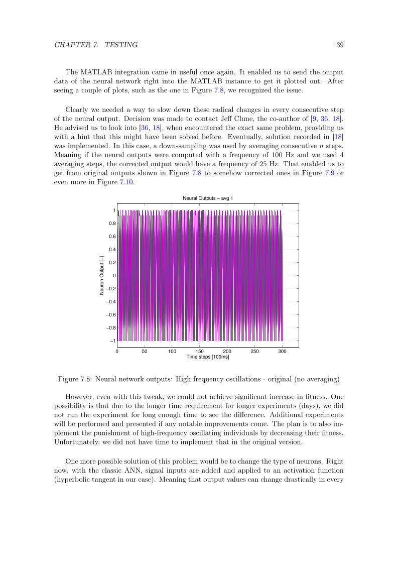
The MATLAB integration came in useful once again. It enabled us to send the outputdata of the neural network right into the MATLAB instance to get it plotted out. Afterseeing a couple of plots, such as the one in Figure 7.8, we recognized the issue.
Clearly we needed a way to slow down these radical changes in every consecutive stepof the neural output. Decision was made to contact Jeff Clune, the co-author of [9, 36, 18].He advised us to look into [36, 18], when encountered the exact same problem, providing uswith a hint that this might have been solved before. Eventually, solution recorded in [18]was implemented. In this case, a down-sampling was used by averaging consecutive n steps.Meaning if the neural outputs were computed with a frequency of 100 Hz and we used 4averaging steps, the corrected output would have a frequency of 25 Hz. That enabled us toget from original outputs shown in Figure 7.8 to somehow corrected ones in Figure 7.9 oreven more in Figure 7.10.
0 50 100 150 200 250 300
−1
−0.8
−0.6
−0.4
−0.2
0
0.2
0.4
0.6
0.8
1
Neural Outputs − avg 1
Time steps [100ms]
Ne
uro
n O
utp
ut
[−]
Figure 7.8: Neural network outputs: High frequency oscillations - original (no averaging)
However, even with this tweak, we could not achieve significant increase in fitness. Onepossibility is that due to the longer time requirement for longer experiments (days), we didnot run the experiment for long enough time to see the difference. Additional experimentswill be performed and presented if any notable improvements come. The plan is to also im-plement the punishment of high-frequency oscillating individuals by decreasing their fitness.Unfortunately, we did not have time to implement that in the original version.
One more possible solution of this problem would be to change the type of neurons. Rightnow, with the classic ANN, signal inputs are added and applied to an activation function(hyperbolic tangent in our case). Meaning that output values can change drastically in every

CHAPTER 7. TESTING 40
0 20 40 60 80 100 120 140 160
−1
−0.8
−0.6
−0.4
−0.2
0
0.2
0.4
0.6
0.8
1
Neural Outputs − avg 2
Time steps [200ms]
Ne
uro
n O
utp
ut
[−]
Figure 7.9: Neural network outputs: High frequency oscillations - averaging 2 consecutivesamples
time step. However, for simulating real-life objects, such as robot legs, an integrating neuroncould be more efficient. Real-life objects cannot move infinitely fast, they only apply forceand gradually change their position. With an integrating neuron, the activation functionwould not provide an absolute value of the neuron for the current time step, but wouldrather provide a change in the current value. Thus the absolute output value of a neuronat time t would be the sum of the absolute value at time t−1 and the relative value at time t.
I represents the set of input synapses.
rel[t] = tanh∑i∈I
signal(i) (7.2)
abs[t] = abs[t− 1] + rel[t] (7.3)
This tweak would forbid the neurons from outputting unreal updated positions for real-life objects. This, as well, is a subject of future research.
7.3.2.2 Neuron output saturation
Another issue that can be seen in Figure 7.8 is the output saturation. Since the activationfunction of the hidden and output neurons is hyperbolic tangent (Figure 7.11), meaning thateven very large inputs are transferred into outputs between -1 and 1. However, the fartherthe inputs are from 0, the less difference on the input gets transferred to the output.
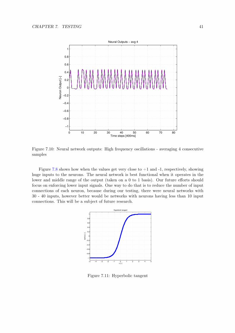
CHAPTER 7. TESTING 41
0 10 20 30 40 50 60 70 80
−1
−0.8
−0.6
−0.4
−0.2
0
0.2
0.4
0.6
0.8
1
Neural Outputs − avg 4
Time steps [400ms]
Ne
uro
n O
utp
ut
[−]
Figure 7.10: Neural network outputs: High frequency oscillations - averaging 4 consecutivesamples
Figure 7.8 shows how when the values get very close to +1 and -1, respectively, showinghuge inputs to the neurons. The neural network is best functional when it operates in thelower and middle range of the output (taken on a 0 to 1 basis). Our future efforts shouldfocus on enforcing lower input signals. One way to do that is to reduce the number of inputconnections of each neuron, because during our testing, there were neural networks with30 - 40 inputs, however better would be networks with neurons having less than 10 inputconnections. This will be a subject of future research.
−5 −4 −3 −2 −1 0 1 2 3 4 5
−1
−0.8
−0.6
−0.4
−0.2
0
0.2
0.4
0.6
0.8
1
Hyperbolic tangent
x [−]
tanh(x
) [−
]
Figure 7.11: Hyperbolic tangent
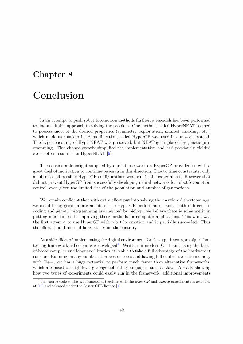
Chapter 8
Conclusion
In an attempt to push robot locomotion methods further, a research has been performedto find a suitable approach to solving the problem. One method, called HyperNEAT seemedto possess most of the desired properties (symmetry exploitation, indirect encoding, etc.)which made us consider it. A modification, called HyperGP was used in our work instead.The hyper-encoding of HyperNEAT was preserved, but NEAT got replaced by genetic pro-gramming. This change greatly simplified the implementation and had previously yieldedeven better results than HyperNEAT [6].
The considerable insight supplied by our intense work on HyperGP provided us with agreat deal of motivation to continue research in this direction. Due to time constraints, onlya subset of all possible HyperGP configurations were run in the experiments. However thatdid not prevent HyperGP from successfully developing neural networks for robot locomotioncontrol, even given the limited size of the population and number of generations.
We remain confident that with extra effort put into solving the mentioned shortcomings,we could bring great improvements of the HyperGP performance. Since both indirect en-coding and genetic programming are inspired by biology, we believe there is some merit inputting more time into improving these methods for computer applications. This work wasthe first attempt to use HyperGP with robot locomotion and it partially succeeded. Thusthe effort should not end here, rather on the contrary.
As a side effect of implementing the digital environment for the experiments, an algorithm-testing framework called cic was developed1. Written in modern C++ and using the best-of-breed compiler and language libraries, it is able to take a full advantage of the hardware itruns on. Running on any number of processor cores and having full control over the memorywith C++, cic has a huge potential to perform much faster than alternative frameworks,which are based on high-level garbage-collecting languages, such as Java. Already showinghow two types of experiments could easily run in the framework, additional improvements
1The source code to the cic framework, together with the hyperGP and symreg experiments is availableat [10] and released under the Lesser GPL licence [1].
42

CHAPTER 8. CONCLUSION 43
to cic’s codebase are in the pipeline.
In addition, cic has been offered to the scientific community as an open-source project,enabling anyone to use it for their experiments. The goal of making cic widely useful hasbeen kept in our minds from the beginning, influencing the block-like design of the insideworkings. Any alternative algorithm can be tested in the same environment by merely plug-ging in new blocks. We have a vision of what cic could become if guided correctly and we seemany experimenters wanting to test their algorithms without the need to write thousandsof lines of code. The MATLAB integration, xml serialization and more is built-in for anyoneto use. We believe researchers should spend more time on improving their ideas and less onbattling programming bugs.
Overall, this work discovered the strengths and weaknesses of HyperGP when appliedto the robot locomotion problem. Many improvements have been suggested and will betested in the future. Experiments have shown that HyperGP is suitable for developingrobot locomotion solutions. In the future, the cic framework should enable us to improvethe HyperGP algorithm and overcome the issues we encountered so far. Moving HyperGPforward should help us explore the true capabilities of computer optimization and find itsnew, truly useful applications.
Bibliography
[1] Lesser GPL Licence, 2013. Source: <http://www.gnu.org/licenses/lgpl.html>.
[2] Simulator Robot 3D, 2013. Source: <http://www.symbrion.eu/tiki-index.php?page=Simulator>.
[3] Sublime Text, 2013. Source: <http://www.sublimetext.com/2>.
[4] APPLE, I. Grand Central Dispatch (GCD) Reference, 2013. Source:<http://developer.apple.com/library/ios/#documentation/Performance/Reference/GCD_libdispatch_Ref/Reference/reference.html>.
[5] APPLE, I. Xcode 4 Downloads and Resources, 2013. Source: <https://developer.apple.com/xcode/>.
[6] BUK, Z. – KOUTNíK, J. – ŠNOREK, M. NEAT in HyperNEAT Substituted withGenetic Programming, 5495 / Lecture Notes in Computer Science, 25, s. 243–252.Springer Berlin Heidelberg, 2009.
[7] CERNY, J. Evolutionary Design of Robot Motion Patterns. Masters Thesis, 2012.http://cyber.felk.cvut.cz/research/theses/papers/226.pdf.
[8] CLICK, D. C. Java vs. C Performance. . . .Again, 2009. Source: <http://www.azulsystems.com/blog/cliff/2009-09-06-java-vs-c-performanceagain>.
[9] CLUNE, J. et al. Evolving coordinated quadruped gaits with the HyperNEAT gener-ative encoding. In Evolutionary Computation, 2009. CEC ’09. IEEE Congress on, s.2764–2771.
[10] DVORSKY, J. cic::hyperGP, . Source: <https://bitbucket.org/honzadvorsky/cic-hypergp>.
[11] DVORSKY, J. hyperGP, . Source: <http://honzadvorsky.com/hypergp/>.
[12] HOWELL, M. Homebrew: The missing package manager for OS X. Source: <http://mxcl.github.io/homebrew/>.
[13] JELOVIC, D. Why Java Will Always Be Slower than C++. Source: <http://www.jelovic.com/articles/why_java_is_slow.htm>.
44
BIBLIOGRAPHY 45
[14] KAMIMURA, A. et al. Automatic locomotion pattern generation for modular robots. InRobotics and Automation, 2003. Proceedings. ICRA ’03. IEEE International Conferenceon, 1, s. 714–720 vol.1.
[15] KIM, O. How many cells are there in the humanbody? Source: <http://www.microbehunter.com/2010/12/17/how-many-cells-are-there-in-the-human-body/>.
[16] KOZA, J. R. Genetic programming: on the programming of computers by means ofnatural selection. MIT Press, 1992.
[17] LARABEL, M. GCC 4.6/4.7 vs. LLVM-Clang 3.0/3.1 Compilers, 2012. Source: <http://www.phoronix.com/scan.php?page=news_item&px=MTA5Nzc>.
[18] LEE, S. et al. Evolving Gaits for Physical Robots with the HyperNEAT GenerativeEncoding: The Benefits of Simulation. In Applications of Evolutionary Computation.Springer, 2013. s. 540–549.
[19] LEWIS, M. A. – FAGG, A. H. – BEKEY, G. A. Genetic Algorithms for Gait Synthesisin a Hexapod Robot. 1994.
[20] LLVM. The LLVM Compiler Infrastructure, 2013. Source: <http://llvm.org>.
[21] LLVM. "libc++" C++ Standard Library, 2013. Source: <http://libcxx.llvm.org>.
[22] LUKE, S. Two fast tree-creation algorithms for genetic programming. EvolutionaryComputation, IEEE Transactions on. 2000, 4, 3, s. 274–283. ISSN 1089-778X. doi:10.1109/4235.873237.
[23] MATHWORKS. MATLAB - The Language of Technical Computing, 2013. Source:<http://www.mathworks.com/products/matlab/>.
[24] ODE. Open Dynamics Engine. Source: <http://www.ode.org>.
[25] OPENPANEL. The Seeming Paradox of the Popularity ofXML, 2008. Source: <http://www.openpanel.com/2008/02/the-seeming-paradox-of-the-popularity-of-xml-2/>.
[26] OSG. OpenSceneGraph. Source: <http://www.openscenegraph.org/projects/osg>.
[27] PROJECT, H. G. How Many Genes Are in the Human Genome? Source: <http://www.ornl.gov/sci/techresources/Human_Genome/faq/genenumber.shtml>.
[28] SIEBEL, N. T. – SOMMER, G. Evolutionary reinforcement learning of artificial neuralnetworks. International Journal of Hybrid Intelligent Systems. 2007, s. 171–183.
[29] SILICONINDIA. 10 Most Popular Programming Languages, 2012. Source: <http://www.siliconindia.com/news/technology/10_Most_Popular_Programming_Languages-nid-106545-cid-2.html>.
BIBLIOGRAPHY 46
[30] SILVA, S. – COSTA, E. Dynamic limits for bloat control in genetic programming and areview of past and current bloat theories. Genetic Programming and Evolvable Machines.2009, 10, 2, s. 141–179.
[31] SIM. sim: Main page, 2012. Source: <http://lynx1.felk.cvut.cz/~danfis/sim-doc/>.
[32] STANLEY, K. O. – D’AMBROSIO, D. B. – GAUCI, J. A hypercube-based encodingfor evolving large-scale neural networks. Artif Life. 2009, 15, 2, s. 185–212. Stanley,Kenneth O D’Ambrosio, David B Gauci, Jason Artif Life. 2009 Spring;15(2):185-212.
[33] W3C. Extensible Markup Language (XML), 2012. Source: <http://www.w3.org/XML/>.
[34] WOLFRAMALPHA. World’s fastest computer, 2012. Source: <http://www.wolframalpha.com/input/?i=worlds+fastest+computer>.
[35] XMLSOFT. The XML C parser and toolkit of Gnome, 2013. Source: <http://www.xmlsoft.org>.
[36] YOSINSKI, J. et al. Evolving robot gaits in hardware: the hyperneat generative en-coding vs. parameter optimization. In Proceedings of the 20th European Conference onArtificial Life, Paris, France, 8, s. 12, 2011.

Appendix A
Important terms and abbreviations
Genotype genetic material of a robot, can always be decoded into one or more phenotypes
Phenotype expression (manifestation) of genotype in particular environment
ANN artificial neural network (or just neural network), mathematical model inspired bybiological neural networks
NEAT Neuro-Evolution of Augmented Topologies, an algorithm for evolving neural net-works
HyperNEAT NEAT algorithm employing hypercube encoding
GP genetic programming, a genetic algorithm using tree-like structures as the genotype
HyperGP GP employing hypercube encoding, first named in [6]
EANT2 Evolutionary Acquisition of Neural Topologies, Version 2
CPPN, CPPF Compositional Pattern Producing Network / Function, the genotype ofHyperNEAT / HyperGP
GCD Grand Central Dispatch - multithread control system for C++ developed by Apple,Inc.
Clang/LLVM C/C++/Objective-C compiler developed by Apple, Inc.
PTC1 Probabilistic Tree-Creation, version 1, a tree-generation method with extra controlover parameters of generated trees
47

Appendix B
Experimental setup
The detailed setup of experiments mentioned in Chapter 7. Each key has its desired statesaved in an xml file with appendix _settings.xml. Experiments used this file to set the desiredstate for the run. The settings file had several major categories, namely GP for geneticprogramming, Simulator for simulation-specific settings, Control for more implementation-specific data, BloatControl for setting up the Bloat Control block and Neural for globalvariables used in neural networks.
Table B.1: Experiment parameters
Parameter key Used value(s) DescriptionGPdefaultFitness 1.0 The default fitness value of in-
dividuals before they are eval-uated.
generatedPopulationSize 50 The number of individuals ineach generation.
expectedGeneratedTreeSize 30 Tree generation parametermentioned in Section 6.3.4.4.
maximumGeneratedTreeDepth 6 Tree generation parameter,maximum allowed depth ofgenerated trees.
minimumGeneratedTreeDepth 2 Tree generation parameter,minimum allowed depth ofgenerated trees.
terminalVariableCount 4 Number of tree variables interminals. HyperGP used[x1, y1, x2, y2].
functionCount 5 Number of tree functions innodes. HyperGP used [x +y, x ∗ y, atan(x), sin(x), e−x2 ].
48

APPENDIX B. EXPERIMENTAL SETUP 49
functionProbabilities all = 1.0 Relative occurencies of func-tions in trees (for PTC1), Sec-tion 6.3.4.4.
functionProbabilities all = 1.0 Relative occurencies of func-tions in trees (for PTC1), Sec-tion 6.3.4.4.
terminalConstsCount 2 Number of extra terminals- constant numbers for treegeneration. HyperGP used[1.0,−1.0].
tournament_size 5 Number of individuals inTournament selection used inGP.
selection_type 0, 1 GP selection type. 0: Tourna-ment, 1: Roulette.
tournamentSelection 1 If two individuals have thesame fitness, select the smallerone (use lexicographic parsi-mony pressure).
numberOfTreesInForestGenotype 1, 4 Described in detail in Sec-tion 7.3.1.
preventDuplicates 1 Generated trees are guaran-teed to be unique.
Simulatorsample_from 0.0 Simulation start time.sample_step 0.5s, 0.0125s The simulator time quan-
tum. Marks re-calculation fre-quency of new outputs. Dis-cussed in Section 7.2.3.
sample_to 15.0 Simulation stop time.delayed_start 2.0 Mark the robot position with
a delay, mentioned in Sec-tion 7.1.2.
robot_type 0, 1, 2 Robot type, as described inSection 7.1.1.
extraTimeStepDivider 1, 20 For cases with low refresh fre-quency, simulation still had torun faster to generate sensi-ble results. This parametermarked how much faster sim-ulation should be computedthan the frequency of outputrecalculations.

APPENDIX B. EXPERIMENTAL SETUP 50
generatePovrayFiles 0, 1 Would be turned on if wewanted to generate files to ren-der video from the simulation.
ControlmaximumIterations 50 The maximum number of gen-
erations / iterations.minimumFitness 50 The minimum fitness reached
to stop the experiment prema-turely. Never used with Hy-perGP.
populationXmlLoadFrom $path of population xml$ Input population into the ex-periment if we did not wanta new population generatedbut continue with a developedone.
useMatlabPlot 0, 1 Turned on if we wanted togenerate plots with statisticsfrom the experiment.
isAutonomousExperiment 0, 1 Turned on to never showthe simulator visually (whichpauses the experiment).
BloatControluseBloatControl 1 Whether bloat control should
be used with the experiment.Discussed in Section 5.2.
bloatControlVariant 0, 1, 2 Version of Dynamics Limitbloat control. 0: simple, 1:heavy, 2: very heavy.
NeuralsynopsisThreshold 0.2 Minimum synapsis absolute
value to be present in the sub-strate (otherwise not added).
useMiddleLegs 0, 1 Whether robot should use its4 or 6-leg variant.
sampleAverageCount 1, 4 Consecutive sample averaging- explained in Section 7.3.2.1.

Appendix C
Attached CD content
The printed version of this work is accompanied by a CD.
README.md File describing the CD content.
cic_2013may20.zip Snapshot of the cic source code.
dvorsky_bt.pdf The text of the bachelor thesis.
videos/ Folder containing several rendered videos of robots from the testing phase.
51


![Chapter [6] Strategy Implementation and Control Strategy Implementation and Control.](https://static.fdocuments.in/doc/165x107/56649cdb5503460f949a5895/chapter-6-strategy-implementation-and-control-strategy-implementation-and.jpg)