NeuralSim: Augmenting Differentiable Simulatorswith Neural Networks

Eric Heiden∗1, David Millard∗1, Erwin Coumans2, Yizhou Sheng1, Gaurav S. Sukhatme1,3

Abstract— Differentiable simulators provide an avenue forclosing the sim-to-real gap by enabling the use of efficient,gradient-based optimization algorithms to find the simulationparameters that best fit the observed sensor readings. Nonethe-less, these analytical models can only predict the dynamicalbehavior of systems for which they have been designed. Inthis work, we study the augmentation of a novel differentiablerigid-body physics engine via neural networks that is ableto learn nonlinear relationships between dynamic quantitiesand can thus model effects not accounted for in traditionalsimulators. Such augmentations require less data to train andgeneralize better compared to entirely data-driven models.Through extensive experiments, we demonstrate the ability ofour hybrid simulator to learn complex dynamics involving fric-tional contacts from real data, as well as match known models ofviscous friction, and present an approach for automatically dis-covering useful augmentations. We show that, besides benefitingdynamics modeling, inserting neural networks can acceleratemodel-based control architectures. We observe a ten-fold speed-up when replacing the QP solver inside a model-predictive gaitcontroller for quadruped robots with a neural network, allowingus to significantly improve control delays as we demonstrate inreal-hardware experiments. We publish code, additional resultsand videos from our experiments on our project webpage athttps://sites.google.com/usc.edu/neuralsim.

I. INTRODUCTION

Physics engines enable the accurate prediction of dynam-ical behavior of systems for which an analytical model hasbeen implemented. Given such models, Bayesian estimationapproaches [1] can be used to find the simulation parametersthat best fit the real-world observations of the given system.While the estimation of simulation parameters for traditionalsimulators via black-box optimization or likelihood-free in-ference algorithms often requires a large number of trainingdata and model evaluations, differentiable simulators allowthe use of gradient-based optimizers that can significantlyimprove the speed of parameter inference approaches [2].

Nonetheless, a sim-to-real gap remains for most systemswe use in the real world. For example, in typical simulationsused in robotics, the robot is assumed to be an articulatedmechanism with perfectly rigid links, even though theyactually bend under heavy loads. Motions are often optimized

∗Equal contribution1Department of Computer Science, University of Southern Cali-

fornia, Los Angeles, USA {heiden, dmillard, yizhoush,gaurav}@usc.edu

2Robotics at Google, Mountain View, USAerwincoumans@google.com

3G.S. Sukhatme holds concurrent appointments as a Professor at USCand as an Amazon Scholar. This paper describes work performed at USCand is not associated with Amazon.

This work was supported by a Google PhD Fellowship and a NASASpace Technology Research Fellowship, grant number 80NSSC19K1182.

Neural QP Controller

OSQP Controller

Neural QP Controller

OSQP Controller

Fig. 1: Top: Snapshots from a few seconds of the locomotion trajectoriesgenerated by the QP-based model-predictive controller (first row) and theneural network controller imitating the QP solver (second row) in ourdifferentiable simulator running the Laikago quadruped. Bottom: model-predictive control using the neural network (third row) and OSQP (fourthrow) running on a real Unitree A1 robot.

without accounting for air resistance. In this work, we focuson overcoming such errors due to unmodeled effects byimplementing a differentiable rigid-body simulator that isenriched by fine-grained data-driven models.

Instead of learning the error correction between the simu-lated and the measured states, as is done in residual physicsmodels, our augmentations are embedded inside the physicsengine. They depend on physically meaningful quantities andactively influence the dynamics by modulating forces andother state variables in the simulation. Thanks to the end-to-end differentiability of our simulator, we can efficiently trainsuch neural networks via gradient-based optimization.

Our experiments demonstrate that the hybrid simulationapproach, where data-driven models augment an analyticalphysics engine at a fine-grained level, outperforms deeplearning baselines in training efficiency and generalizability.The hybrid simulator is able to learn a model for the dragforces for a swimmer mechanism in a viscous mediumwith orders of magnitude less data compared to a sequencelearning model. When unrolled beyond the time steps ofthe training regime, the augmented simulator significantlyoutperforms the baselines in prediction accuracy. Such ca-pability is further beneficial to closing the sim-to-real gap.We present results for planar pushing where the contactfriction model is enriched by neural networks to closelymatch the observed motion of an object being pushed in thereal world. Leveraging techniques from sparse regression,

arX

iv:2

011.

0421

7v2

[cs

.RO

] 1

9 M

ay 2

021

Analytical Data-driven End-to-end ∇ Hybrid

Physics engine [3], [4], [5] XResidual physics [6], [7], [8], [9] X X XLearned physics [10], [11], [12], [13] X XDifferentiable simulators [14], [15], [16], [17], [18], [19], [2] X XOur approach X X X X

TABLE I: Comparison of dynamics modeling approaches (selected works) along the axes of analytical and data-drivenmodeling, end-to-end differentiability, and hybrid approaches.

we can identify which inputs to the data-driven models arethe most relevant, giving the opportunity to discover placeswhere to insert such neural augmentations.

Besides reducing the modeling error or learning entirelyunmodeled effects, introducing neural networks to the com-putation pipeline can have computational benefits. In real-robot experiments on a Unitree A1 quadruped we show thatwhen the quadratic programming (QP) solver of a model-predictive gait controller is replaced by a neural network,the inference time can be reduced by an order of magnitude.

We release our novel, open-source physics engine, TinyDifferentiable Simulator (TDS)1, which implements articu-lated rigid-body dynamics and contact models, and supportsvarious methods of automatic differentiation to computegradients w.r.t. any quantity inside the engine.

II. RELATED WORK

Various methods have been proposed to learn systemdynamics from time series data of real systems (see Table Iand Figure 2 left). Early works include Locally WeightedRegression [20] and Forward Models [21]. Modern “intuitivephysics” models often use deep graph neural networks todiscover constraints between particles or bodies ([11], [22],[23], [24], [25], [26], [12], [27]). Physics-based machinelearning approaches introduce a physics-informed inductivebias to the problem of learning models for dynamical systemsfrom data [28], [29], [30], [31], [32], [33]. We propose ageneral-purpose hybrid simulation approach that combinesanalytical models of dynamical systems with data-drivenresidual models that learn parts of the dynamics unaccountedfor by the analytical simulation models.

Originating from traditional physics engines (examplesinclude [3], [4], [5]), differentiable simulators have beenintroduced that leverage automatic, symbolic or implicitdifferentiation to calculate parameter gradients through theanalytical Newton-Euler equations and contact models forrigid-body dynamics [14], [16], [17], [34], [35], [36], [18],[37], [38]. Simulations for other physical processes, such aslight propagation [39], [40] and continuum mechanics [41],[42], [15], [19], [2] have been made differentiable as well.

Residual physics models [8], [7], [6], [9] augment physicsengines with learned models to reduce the sim-to-real gap.Most of them introduce residual learning applied from theoutside to the predicted state of the physics engine, whilewe propose a more fine-grained approach, similar to [6],where data-driven models are introduced only at some parts

1Open-source release of TDS: https://github.com/google-research/tiny-differentiable-simulator

in the simulator. While in [6] the network for actuatordynamics is trained through supervised learning, our end-to-end differentiable model allows backpropagation of gradientsfrom high-level states to any part of the computation graph,including neural network weights, so that these parameterscan be optimized efficiently, for example from end-effectortrajectories.

III. APPROACH

Our simulator implements the Articulated Body Algorithm(ABA) [43] to compute the forward dynamics (FD) forarticulated rigid-body mechanisms. Given joint positionsq, velocities q, torques τ in generalized coordinates, andexternal forces fext, ABA calculates the joint accelerationsq. We use semi-implicit Euler integration to advance thesystem dynamics in time. We support two types of contactmodels: an impulse-level solver that uses a form of theProjected Gauss Seidel algorithm [44], [45] to solve a non-linear complementarity problem (NCP) to compute contactimpulses for multiple simultaneous points of contact, anda penalty-based contact model that computes joint forcesindividually per contact point via the Hunt-Crossley [46]nonlinear spring-damper system. In addition to the contactnormal force, the NCP-based model resolves lateral frictionfollowing Coulomb’s law, whereas the spring-based modelimplements a nonlinear friction force model following Brownet al. [47].

Each link i in a rigid-body system has a mass value mi,an inertia tensor Ii ∈ R6×6, and a center of mass hi ∈ R6×6.Each corresponding nd degree of freedom joint i betweenlink i and its parent λ (i) has a spring stiffness coefficientki, a damping coefficient di, a transformation from its axisto its parent λ (i)Xi ∈ SE(3), and a motion subspace matrixSi ∈ R6×nd .

For problems involving nc possible contacts, each possiblepair j of contacts has a friction coefficient µ j ∈R describingthe shape of the Coulomb friction cone. Additionally, tomaintain contact constraints during dynamics integration, weuse Baumgarte stabilization [48] with parameters α j,β j ∈R.To soften the shape of the contact NCP, we use ConstraintForce Mixing (CFM), a regularization technique with param-eters R j ∈ Rnc .

θAM = {mi,Ii,hi,λ (i)Xi,Si}i ∪ {µ j,α j,β j,R j} j

are the analytical model parameters of the system, whichhave an understandable and physically relevant effect on thecomputed dynamics. Any of the parameters in θAM may bemeasurable with certainty a priori, or can be optimized as

Analytical Model Data-driven Model Residual Physics Hybrid Simulation

PhysicsEngine

LearnedModel

LearnedModel

PhysicsEngine

Hybrid Simulator

Fig. 2: Left: comparison of various model architectures (cf. Anurag et al. [7]). Right: augmentation of differentiable simulators with our proposed neuralscalar type where variable e becomes a combination of an analytical model φ(·, ·) with inputs a and b, and a neural network whose inputs are a, c, and d.

Integrator Forward Dynamics

Fig. 3: Exemplar architecture of our hybrid simulator where a neural networklearns passive forces τ given joint velocities q (MLP biases and jointpositions q are not shown).

part of a system identification problem according to somedata-driven loss function.

With these parameters, we view the dynamics of thesystem as

τ = HθAM (q)q+CθAM (q, q)+gθAM (q) (1)

where HθAM computes the generalized inertia matrix of thesystem, CθAM computes nonlinear Coriolis and centrifugaleffects, and gθAM describes passive forces and forces due togravity.

A. Hybrid Simulation

Even if the best-fitting analytical model parameters havebeen determined, rigid-body dynamics alone often does notexactly predict the motion of mechanisms in the real world.To address this, we propose a technique for hybrid simula-tion that leverages differentiable physics models and neuralnetworks to allow the efficient reduction of the simulation-to-reality gap. By enabling any part of the simulation to bereplaced or augmented by neural networks with parametersθNN , we can learn unmodeled effects from data which theanalytical models do not account for.

Our physics engine allows any variable participating inthe simulation to be augmented by neural networks thataccept input connections from any other variable. In thesimulation code, such neural scalars (Figure 2 right) areassigned a unique name, so that in a separate experimentcode a “neural blueprint” is defined that declares the neuralnetwork architectures and sets the network weights.

ParameterError

Local Optimization Parallel Basin Hopping

Fig. 4: Comparison of system identification results from local optimization(left) and the parallel basin hopping strategy (right), where the grid cellsindicate the initial parameters from which the optimization was started. Thelink lengths of a double pendulum are the two simulation parameters to beestimated from joint position trajectories. The true parameters are 3 and 4(indicated by a star), and the colors indicate the `2 distance between theground truth and the parameters obtained after optimization (darker shadeindicates lower error).

B. Overcoming Local Minima

For problems involving nonlinear or discontinuous sys-tems, such as rigid-body mechanisms undergoing contact,our strategy yields highly nonlinear loss landscape whichis fraught with local minima. As such, we employ globaloptimization strategies, such as the parallel basin hoppingstrategy [49] and population-based techniques from thePagmo library [50]. These global approaches run a gradient-based optimizer, such as L-BFGS in our case, locally ineach individual thread. After each evolution of a populationof local optimizers, the best solutions are combined andmutated so that in the next evolution each optimizer startsfrom a newly generated parameter vector. As can be seenin Figure 4, a system identification problem as basic asestimating the link lengths of a double pendulum froma trajectory of joint positions, results in a complex losslandscape where a purely local optimizer often only findssuboptimal parameters (left). Parallel Basin Hopping (right),on the other hand, restarts multiple local optimizers with aninitial value around the currently best found solution, therebyovercoming poor local minima in the loss landscape.

C. Implementation Details

We implement our physics engine Tiny DifferentiableSimulator (TDS) in C++ while keeping the computationsagnostic to the implementation of linear algebra structuresand operations. Via template meta-programming, various

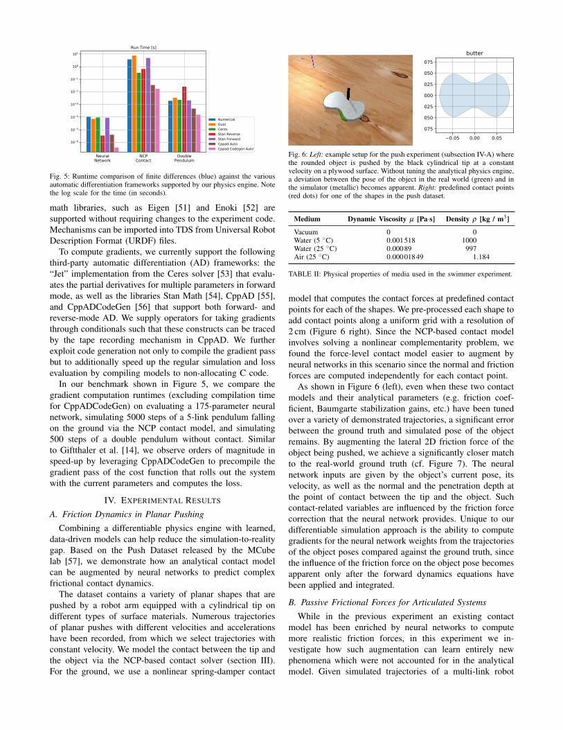
Fig. 5: Runtime comparison of finite differences (blue) against the variousautomatic differentiation frameworks supported by our physics engine. Notethe log scale for the time (in seconds).

math libraries, such as Eigen [51] and Enoki [52] aresupported without requiring changes to the experiment code.Mechanisms can be imported into TDS from Universal RobotDescription Format (URDF) files.

To compute gradients, we currently support the followingthird-party automatic differentiation (AD) frameworks: the“Jet” implementation from the Ceres solver [53] that evalu-ates the partial derivatives for multiple parameters in forwardmode, as well as the libraries Stan Math [54], CppAD [55],and CppADCodeGen [56] that support both forward- andreverse-mode AD. We supply operators for taking gradientsthrough conditionals such that these constructs can be tracedby the tape recording mechanism in CppAD. We furtherexploit code generation not only to compile the gradient passbut to additionally speed up the regular simulation and lossevaluation by compiling models to non-allocating C code.

In our benchmark shown in Figure 5, we compare thegradient computation runtimes (excluding compilation timefor CppADCodeGen) on evaluating a 175-parameter neuralnetwork, simulating 5000 steps of a 5-link pendulum fallingon the ground via the NCP contact model, and simulating500 steps of a double pendulum without contact. Similarto Giftthaler et al. [14], we observe orders of magnitude inspeed-up by leveraging CppADCodeGen to precompile thegradient pass of the cost function that rolls out the systemwith the current parameters and computes the loss.

IV. EXPERIMENTAL RESULTS

A. Friction Dynamics in Planar Pushing

Combining a differentiable physics engine with learned,data-driven models can help reduce the simulation-to-realitygap. Based on the Push Dataset released by the MCubelab [57], we demonstrate how an analytical contact modelcan be augmented by neural networks to predict complexfrictional contact dynamics.

The dataset contains a variety of planar shapes that arepushed by a robot arm equipped with a cylindrical tip ondifferent types of surface materials. Numerous trajectoriesof planar pushes with different velocities and accelerationshave been recorded, from which we select trajectories withconstant velocity. We model the contact between the tip andthe object via the NCP-based contact solver (section III).For the ground, we use a nonlinear spring-damper contact

Fig. 6: Left: example setup for the push experiment (subsection IV-A) wherethe rounded object is pushed by the black cylindrical tip at a constantvelocity on a plywood surface. Without tuning the analytical physics engine,a deviation between the pose of the object in the real world (green) and inthe simulator (metallic) becomes apparent. Right: predefined contact points(red dots) for one of the shapes in the push dataset.

Medium Dynamic Viscosity µ [Pa·s] Density ρ [kg / m3]

Vacuum 0 0Water (5 ◦C) 0.001518 1000Water (25 ◦C) 0.00089 997Air (25 ◦C) 0.00001849 1.184

TABLE II: Physical properties of media used in the swimmer experiment.

model that computes the contact forces at predefined contactpoints for each of the shapes. We pre-processed each shape toadd contact points along a uniform grid with a resolution of2 cm (Figure 6 right). Since the NCP-based contact modelinvolves solving a nonlinear complementarity problem, wefound the force-level contact model easier to augment byneural networks in this scenario since the normal and frictionforces are computed independently for each contact point.

As shown in Figure 6 (left), even when these two contactmodels and their analytical parameters (e.g. friction coef-ficient, Baumgarte stabilization gains, etc.) have been tunedover a variety of demonstrated trajectories, a significant errorbetween the ground truth and simulated pose of the objectremains. By augmenting the lateral 2D friction force of theobject being pushed, we achieve a significantly closer matchto the real-world ground truth (cf. Figure 7). The neuralnetwork inputs are given by the object’s current pose, itsvelocity, as well as the normal and the penetration depth atthe point of contact between the tip and the object. Suchcontact-related variables are influenced by the friction forcecorrection that the neural network provides. Unique to ourdifferentiable simulation approach is the ability to computegradients for the neural network weights from the trajectoriesof the object poses compared against the ground truth, sincethe influence of the friction force on the object pose becomesapparent only after the forward dynamics equations havebeen applied and integrated.

B. Passive Frictional Forces for Articulated Systems

While in the previous experiment an existing contactmodel has been enriched by neural networks to computemore realistic friction forces, in this experiment we in-vestigate how such augmentation can learn entirely newphenomena which were not accounted for in the analyticalmodel. Given simulated trajectories of a multi-link robot

Fig. 7: Trajectories of pushing an ellipsoid object from our hybrid simulator(blue) and the non-augmented rigid-body simulation (orange) comparedagainst the real-world ground truth from the MCube push dataset [57]. Theshaded ellipsoids indicate the final object poses.

Fig. 8: Left: Model of a swimmer in MuJoCo with five revolute jointsconnecting its links simulated as capsules interacting with ambient fluid.Right: Evolution of the cost function during the training of the neural-augmented simulator for the swimmer in different media.

swimming through an unidentified viscous medium (Fig-ure 8), the augmentation is supposed to learn a model for thepassive forces that describe the effects of viscous friction anddamping encountered in the fluid. Since the passive forcesexerted by a viscous medium are dependent on the angle ofattack of each link, as well as the velocity, we add a neuralaugmentation to τ , ψθ (q, q), analogous to Figure 3.

Using our hybrid physics engine, and given a set ofgeneralized control forces u, we integrate Equation 1 to forma trajectory T = {qi, ˆqi}i, and compute an MSE loss L(T, T )against T , a ground truth trajectory of generalized states andvelocities recorded using the MuJoCo [4] simulator. We areable to compute exact gradients ∇θL end-to-end throughthe entire trajectory, given the differentiable nature of oursimulator, integrator, and function approximator.

We train the hybrid simulator under different ground-truthinputs. We consider water at 5 ◦C and 25 ◦C temperature,plus air at 25 ◦C, as media, which have different propertiesfor dynamic viscosity and density (see Table II).

Leveraging the mechanical structure of problems aids inlong-term physically relevant predictive power, especially inthe extremely sparse data regimes common in learning forrobotics. As shown in Figure 9, our approach, trained end-to-end on the initial 200 timesteps of 10 trajectories of a2-link swimmer moving in water at 25 ◦C, exhibits moreaccurate long-term rollout prediction over 900 timesteps than

a deep long short-term memory (LSTM) network. In thisexperiment, the augmentation networks for TDS have 1637trainable parameters, while the LSTM has 1900.

C. Discovering Neural Augmentations

In our previous experiments we carefully selected whichsimulation quantities to augment by neural networks. Whileit is expected that air resistance and friction result in passiveforces that need to be applied to the simulated mechanism,it is often difficult to foresee which dynamical quantitiesactually influence the dynamics of the observed system.Since we aim to find minimally invasive data-driven mod-els, we focus on neural network augmentations that havethe least possible effect while achieving the goal of highpredictive accuracy and generalizability. Inspired by SparseInput Neural Networks (SPINN) [58], we adapt the sparse-group lasso [59] penalty for the cost function:

L= ∑t|| fθ (st−1)− s∗t ||22 +κ||θ[:1]||1 +λ ||θ[1:]||22, (2)

given weighting coefficients κ,λ > 0, where fθ (st−1) is thestate predicted by the hybrid simulator given the previoussimulation state st−1 (consisting of q, q), s∗t is the state fromthe observed system, θ[:1] are the network weights of thefirst layer, and θ[1:] are the weights of the upper layers.Such cost function sparsifies the input weights so that theaugmentation depends on only a small subset of physicalquantities, which is desirable when simpler models are to befound that potentially overfit less to the training data whilemaintaining high accuracy (Occam’s razor). In addition,the L2 loss on the weights from the upper network layerspenalizes the overall contribution of the neural augmentationto the predicted dynamics since we only want to augment thesimulation where the analytical model is unable to match thereal system.

We demonstrate the approach on a double pendulumsystem that is modeled as a frictionless mechanism inour analytical physics engine. The reference system, onthe other hand, is assumed to exhibit joint friction, i.e.,a force proportional to and opposed to the joint velocity.As expected, compared to a fully learned dynamics model,our hybrid simulator outperforms the baselines significantly(Figure 10). As shown on the right, convergence is achievedwhile requiring orders of magnitude less training samples.At the same time, the resulting neural network augmentationconverges to weights that clearly show that the joint velocityqi influences the residual joint force τi that explains theobserved effects of joint friction in joint i (Figure 10 left).

D. Imitation Learning from MPC

Starting from a rigid-body simulation and augmentingit by neural networks has shown significant improvementsin closing the sim-to-real gap and learning entirely neweffects, such as viscous friction that has not been modeledanalytically. In our final experiment, we investigate howthe use of learned models can benefit a control pipelinefor a quadruped robot. We simulate a Laikago quadruped

Fig. 9: Trajectory of positions q and velocities q of a swimmer in water at 25 ◦C temperature actuated by random control inputs. In a low-data regime, ourapproach (orange) generates accurate predictions, even past the training cutoff (vertical black bar), while an entirely data-driven model (green) regressesto the mean. The behavior of the unaugmented analytical model, which corresponds to a swimmer in vacuum, is shown for comparison.

Fig. 10: Left: Neural augmentation for a double pendulum that learnsjoint damping. Given the fully connected neural network (top), after 15optimization steps using the sparse group lasso cost function (Equation 2)(bottom), the input layer (light green) is sparsified to only the relevantquantities that influence the dynamics of the observed system. Right: Finalmean squared error (MSE) on test data after training a feed-forward neuralnetwork and our hybrid physics engine.

robot and use a model-predictive controller (MPC) to gener-ate walking gaits. The MPC implements [60] and uses aquadratic programming (QP) solver leveraging the OSQPlibrary [61] that computes the desired contact forces at thefeet, given the current measured state of the robot (centerof mass (COM), linear and angular velocity, COM estimatedposition (roll, pitch and yaw), foot contact state as well asthe desired COM position and velocity). The swing feet arecontrolled using PD position control, while the stance feet aretorque-controlled using the QP solver to satisfy the motionconstraints. This controller has been open-sourced as part ofthe quadruped animal motion imitation project [62]2.

We train a neural network policy to imitate the QP solver,taking the same system state as inputs, and predicting thecontact forces at the feet which are provided to the IKsolver and PD controller. As training dataset we recorded 10kstate transitions generated by the QP solver, using randomlinear and angular MPC control targets of the motion of thetorso. We choose a fully connected neural network with 41-dimensional input and two hidden layers of 192 nodes thatoutputs the 12 joint torques, all using ELU activation [63].

The neural network controller is able to produce extensivewalking gaits in simulation for the Laikago robot, and in-place trotting gaits on a real Unitree A1 quadruped (see

2The implementation of the QP-based MPC is available open-source athttps://github.com/google-research/motion_imitation

Figure 1). The learned QP solver is an order of magnitudefaster than the original QP solver (0.2 ms inference timeversus 2 ms on an AMD 3090 Ryzen CPU).

Thanks to improved performance, the control frequencyincreased from 160 Hz to 300 Hz. Since the model wastrained using data only acquired in simulation, there is somesim-to-real gap, causing the robot to trot with a slightlylower torso height. In future work, we plan to leverage ourend-to-end differentiable simulator to fine-tune the policywhile closing the simulation-to-reality gap from real-worldsensor measurements. Furthermore, the use of differentiablesimulators, such as in [64], to train data-driven models withfaster inference times is an exciting direction to speed upconventional physics engines.

V. CONCLUSION

We presented a differentiable simulator for articulatedrigid-body dynamics that allows the insertion of neuralnetworks at any point in the computation graph. Such neuralaugmentation can learn dynamical effects that the analyticalmodel does not account for, while requiring significantlyless training data from the real system. Our experimentsdemonstrate benefits for sim-to-real transfer, for examplein planar pushing where, contrary to the given model, thefriction force depends not only on the objects velocity butalso on its position on the surface. Effects that have notbeen present altogether in the rigid-body simulator, such asdrag forces due to fluid viscosity, can also be learned fromdemonstration. Throughout our experiments, the efficientcomputation of gradients that our implemented simulatorfacilitates, has considerably sped up the training process.Furthermore, replacing conventional components, such as theQP-based controller in our quadruped locomotion experi-ments, has resulted in an order of magnitude computationspeed-up.

In future work we plan to investigate how physicallymeaningful constraints, such as the law of conservation ofenergy, can be incorporated into the training of the neuralnetworks. We will further our preliminary investigation ofdiscovering neural network connections and the viabilityof such techniques on real-world systems, where hybridsimulation can play a key role in model-based control.

ACKNOWLEDGMENTS

We thank Carolina Parada and Ken Caluwaerts for theirhelpful feedback and suggestions.

REFERENCES

[1] F. Ramos, R. C. Possas, and D. Fox, “BayesSim: adaptive domainrandomization via probabilistic inference for robotics simulators,”Robotics: Science and Systems, 2019.

[2] J. K. Murthy, M. Macklin, F. Golemo, V. Voleti, L. Petrini, M. Weiss,B. Considine, J. Parent-Levesque, K. Xie, K. Erleben, L. Paull,F. Shkurti, D. Nowrouzezahrai, and S. Fidler, “gradSim: Differentiablesimulation for system identification and visuomotor control,”in International Conference on Learning Representations, 2021.[Online]. Available: https://openreview.net/forum?id=c E8kFWfhp0

[3] E. Coumans and Y. Bai, “Pybullet, a python module for physicssimulation for games, robotics and machine learning,” 2016–2020.[Online]. Available: http://pybullet.org

[4] E. Todorov, T. Erez, and Y. Tassa, “Mujoco: A physics engine formodel-based control,” in 2012 IEEE/RSJ International Conference onIntelligent Robots and Systems. IEEE, 2012, pp. 5026–5033.

[5] J. Lee, M. X. Grey, S. Ha, T. Kunz, S. Jain, Y. Ye, S. S. Srinivasa,M. Stilman, and C. K. Liu, “Dart: Dynamic animation and roboticstoolkit,” Journal of Open Source Software, vol. 3, no. 22, p. 500,2018. [Online]. Available: https://doi.org/10.21105/joss.00500

[6] J. Hwangbo, J. Lee, A. Dosovitskiy, D. Bellicoso, V. Tsounis,V. Koltun, and M. Hutter, “Learning agile and dynamic motor skillsfor legged robots,” Science Robotics, vol. 4, no. 26, p. eaau5872, 2019.

[7] A. Ajay, J. Wu, N. Fazeli, M. Bauza, L. P. Kaelbling, J. B. Tenenbaum,and A. Rodriguez, “Augmenting Physical Simulators with StochasticNeural Networks: Case Study of Planar Pushing and Bouncing,” inIEEE/RSJ International Conference on Intelligent Robots and Systems(IROS), 2018.

[8] A. Zeng, S. Song, J. Lee, A. Rodriguez, and T. Funkhouser, “Tossing-bot: Learning to throw arbitrary objects with residual physics,” 2019.

[9] F. Golemo, A. A. Taiga, A. Courville, and P.-Y. Oudeyer, “Sim-to-realtransfer with neural-augmented robot simulation,” in Proceedings ofThe 2nd Conference on Robot Learning, ser. Proceedings of MachineLearning Research, A. Billard, A. Dragan, J. Peters, and J. Morimoto,Eds., vol. 87. PMLR, 29–31 Oct 2018, pp. 817–828. [Online].Available: http://proceedings.mlr.press/v87/golemo18a.html

[10] A. Sanchez-Gonzalez, J. Godwin, T. Pfaff, R. Ying, J. Leskovec, andP. W. Battaglia, “Learning to simulate complex physics with graphnetworks,” arXiv preprint arXiv:2002.09405, 2020.

[11] P. Battaglia, R. Pascanu, M. Lai, D. J. Rezende, et al., “Interaction net-works for learning about objects, relations and physics,” in Advancesin Neural Information Processing Systems, 2016, pp. 4502–4510.

[12] Y. Li, J. Wu, R. Tedrake, J. B. Tenenbaum, andA. Torralba, “Learning particle dynamics for manipulatingrigid bodies, deformable objects, and fluids,” in InternationalConference on Learning Representations, 2019. [Online]. Available:https://openreview.net/forum?id=rJgbSn09Ym

[13] Y. Jiang and C. K. Liu, “Data-augmented contact model for rigid bodysimulation,” CoRR, vol. abs/1803.04019, 2018. [Online]. Available:http://arxiv.org/abs/1803.04019

[14] M. Giftthaler, M. Neunert, M. Stauble, M. Frigerio, C. Semini, andJ. Buchli, “Automatic differentiation of rigid body dynamics foroptimal control and estimation,” Advanced Robotics, vol. 31, no. 22,pp. 1225–1237, 2017.

[15] Y. Hu, L. Anderson, T.-M. Li, Q. Sun, N. Carr, J. Ragan-Kelley,and F. Durand, “DiffTaichi: Differentiable programming for physicalsimulation,” ICLR, 2020.

[16] J. Carpentier and N. Mansard, “Analytical derivatives of rigid bodydynamics algorithms,” in Robotics: Science and Systems, 2018.

[17] F. de Avila Belbute-Peres, K. Smith, K. Allen, J. Tenenbaum,and J. Z. Kolter, “End-to-end differentiable physics for learningand control,” in Advances in Neural Information Processing Systems31, S. Bengio, H. Wallach, H. Larochelle, K. Grauman, N. Cesa-Bianchi, and R. Garnett, Eds. Curran Associates, Inc., 2018,pp. 7178–7189. [Online]. Available: http://papers.nips.cc/paper/7948-end-to-end-differentiable-physics-for-learning-and-control.pdf

[18] M. Geilinger, D. Hahn, J. Zehnder, M. Bacher, B. Thomaszewski, andS. Coros, “ADD: Analytically differentiable dynamics for multi-bodysystems with frictional contact,” 2020.

[19] Y.-L. Qiao, J. Liang, V. Koltun, and M. C. Lin, “Scalable differentiablephysics for learning and control,” in ICML, 2020.

[20] S. Schaal and C. G. Atkeson, “Robot juggling: implementation ofmemory-based learning,” IEEE Control Systems Magazine, vol. 14,no. 1, pp. 57–71, 1994.

[21] A. W. Moore, “Fast, robust adaptive control by learning only forwardmodels,” in Proceedings of the 4th International Conference on NeuralInformation Processing Systems, ser. NIPS’91. San Francisco, CA,USA: Morgan Kaufmann Publishers Inc., 1991, p. 571–578.

[22] Z. Xu, J. Wu, A. Zeng, J. B. Tenenbaum, and S. Song, “DensePhysNet:Learning dense physical object representations via multi-step dynamicinteractions,” Robotics: Science and Systems, June 2019.

[23] S. He, Y. Li, Y. Feng, S. Ho, S. Ravanbakhsh, W. Chen, andB. Poczos, “Learning to predict the cosmological structure formation,”Proceedings of the National Academy of Sciences of the United Statesof America, vol. 116, no. 28, pp. 13 825–13 832, July 2019.

[24] M. Raissi, H. Babaee, and P. Givi, “Deep learning of turbulent scalarmixing,” Tech. Rep., 2018.

[25] D. Mrowca, C. Zhuang, E. Wang, N. Haber, L. Fei-Fei, J. B. Tenen-baum, and D. L. K. Yamins, “Flexible neural representation for physicsprediction,” Advances in Neural Information Processing Systems, June2018.

[26] T. Q. Chen, Y. Rubanova, J. Bettencourt, and D. K. Duvenaud, “Neuralordinary differential equations,” in Advances in Neural InformationProcessing Systems, 2018, pp. 6571–6583.

[27] A. Sanchez-Gonzalez, J. Godwin, T. Pfaff, R. Ying, J. Leskovec, andP. W. Battaglia, “Learning to simulate complex physics with graphnetworks,” 2020.

[28] R. T. Q. Chen, Y. Rubanova, J. Bettencourt, and D. K. Duvenaud,“Neural ordinary differential equations,” in Advances in Neural Infor-mation Processing Systems 31, S. Bengio, H. Wallach, H. Larochelle,K. Grauman, N. Cesa-Bianchi, and R. Garnett, Eds. CurranAssociates, Inc., 2018, pp. 6571–6583. [Online]. Available: http://papers.nips.cc/paper/7892-neural-ordinary-differential-equations.pdf

[29] Z. Long, Y. Lu, X. Ma, and B. Dong, “Pde-net: Learning pdes fromdata,” in International Conference on Machine Learning, 2018, pp.3208–3216.

[30] M. Raissi, P. Perdikaris, and G. E. Karniadakis, “Physics-informedneural networks: A deep learning framework for solving forward andinverse problems involving nonlinear partial differential equations,”Journal of Computational Physics, vol. 378, pp. 686–707, 2019.

[31] M. Lutter, C. Ritter, and J. Peters, “Deep Lagrangian networks:Using physics as model prior for deep learning,” arXiv preprintarXiv:1907.04490, 2019.

[32] S. Greydanus, M. Dzamba, and J. Yosinski, “Hamiltonian neuralnetworks,” in Advances in Neural Information Processing Systems32, H. Wallach, H. Larochelle, A. Beygelzimer, F. d'Alche-Buc,E. Fox, and R. Garnett, Eds. Curran Associates, Inc., 2019,pp. 15 379–15 389. [Online]. Available: http://papers.nips.cc/paper/9672-hamiltonian-neural-networks.pdf

[33] G. Sutanto, A. Wang, Y. Lin, M. Mukadam, G. Sukhatme, A. Rai,and F. Meier, “Encoding physical constraints in differentiableNewton-Euler algorithm,” ser. Proceedings of Machine LearningResearch, A. M. Bayen, A. Jadbabaie, G. Pappas, P. A. Parrilo,B. Recht, C. Tomlin, and M. Zeilinger, Eds., vol. 120. TheCloud: PMLR, 10–11 Jun 2020, pp. 804–813. [Online]. Available:http://proceedings.mlr.press/v120/sutanto20a.html

[34] T. Koolen and R. Deits, “Julia for robotics: simulation and real-time control in a high-level programming language,” in InternationalConference on Robotics and Automation, 05 2019.

[35] E. Heiden, D. Millard, H. Zhang, and G. S. Sukhatme, “Interactivedifferentiable simulation,” CoRR, vol. abs/1905.10706, 2019. [Online].Available: http://arxiv.org/abs/1905.10706

[36] E. Heiden, D. Millard, and G. S. Sukhatme, “Real2sim transfer usingdifferentiable physics,” R:SS Workshop on Closing the Reality Gap inSim2real Transfer for Robotic Manipulation, 2019.

[37] Q. Lelidec, I. Kalevatykh, I. Laptev, C. Schmid, and J. Carpentier,“Differentiable simulation for physical system identification,” IEEERobotics and Automation Letters, pp. 1–1, 2021.

[38] M. Lutter, J. Silberbauer, J. Watson, and J. Peters, “Differentiablephysics models for real-world offline model-based reinforcementlearning,” 2020.

[39] M. Nimier-David, D. Vicini, T. Zeltner, and W. Jakob, “Mitsuba 2: Aretargetable forward and inverse renderer,” Transactions on Graphics(Proceedings of SIGGRAPH Asia), vol. 38, no. 6, Nov. 2019.

[40] E. Heiden, Z. Liu, R. K. Ramachandran, and G. S. Sukhatme,“Physics-based simulation of continuous-wave LIDAR for localiza-tion, calibration and tracking,” in International Conference on Roboticsand Automation (ICRA). IEEE, 2020.

[41] Y. Hu, J. Liu, A. Spielberg, J. B. Tenenbaum, W. T. Freeman, J. Wu,D. Rus, and W. Matusik, “Chainqueen: A real-time differentiable phys-ical simulator for soft robotics,” Proceedings of IEEE InternationalConference on Robotics and Automation (ICRA), 2019.

[42] J. Liang, M. Lin, and V. Koltun, “Differentiable cloth simulationfor inverse problems,” in Advances in Neural Information ProcessingSystems, 2019, pp. 771–780.

[43] R. Featherstone, Rigid Body Dynamics Algorithms. Berlin, Heidel-berg: Springer-Verlag, 2007.

[44] D. Stewart and J. C. Trinkle, “An implicit time-stepping schemefor rigid body dynamics with coulomb friction,” in Proceedings2000 ICRA. Millennium Conference. IEEE International Confer-ence on Robotics and Automation. Symposia Proceedings (Cat. No.00CH37065), vol. 1. IEEE, 2000, pp. 162–169.

[45] P. C. Horak and J. C. Trinkle, “On the similarities and differencesamong contact models in robot simulation,” IEEE Robotics andAutomation Letters, vol. 4, no. 2, pp. 493–499, 2019.

[46] K. H. Hunt and F. R. E. Crossley, “Coefficient of restitution interpretedas damping in vibroimpact,” 1975.

[47] P. Brown and J. McPhee, “A 3d ellipsoidal volumetric foot–groundcontact model for forward dynamics,” Multibody System Dynamics,vol. 42, no. 4, pp. 447–467, 2018.

[48] J. Baumgarte, “Stabilization of constraints and integrals of motionin dynamical systems,” Computer methods in applied mechanics andengineering, vol. 1, no. 1, pp. 1–16, 1972.

[49] S. L. McCarty, L. M. Burke, and M. McGuire, “Parallel monotonicbasin hopping for low thrust trajectory optimization,” in 2018 SpaceFlight Mechanics Meeting, 2018, p. 1452.

[50] F. Biscani and D. Izzo, “A parallel global multiobjective framework foroptimization: pagmo,” Journal of Open Source Software, vol. 5, no. 53,p. 2338, 2020. [Online]. Available: https://doi.org/10.21105/joss.02338

[51] G. Guennebaud, B. Jacob, et al., “Eigen v3,” http://eigen.tuxfamily.org,2010.

[52] W. Jakob, “Enoki: structured vectorization and differentiation onmodern processor architectures,” 2019, https://github.com/mitsuba-renderer/enoki.

[53] S. Agarwal, K. Mierle, and Others, “Ceres solver,” http://ceres-solver.org.

[54] B. Carpenter, M. D. Hoffman, M. Brubaker, D. Lee, P. Li, andM. Betancourt, “The Stan math library: Reverse-mode automaticdifferentiation in c++,” arXiv preprint arXiv:1509.07164, 2015.

[55] B. Bell, “CppAD: a package for C++ algorithmic differentiation,”http://www.coin-or.org/CppAD, 2020.

[56] J. R. Leal and B. Bell, “joaoleal/CppADCodeGen: CppAD 2017,”July 2017. [Online]. Available: https://doi.org/10.5281/zenodo.836832

[57] K.-T. Yu, M. Bauza, N. Fazeli, and A. Rodriguez, “More than a millionways to be pushed. a high-fidelity experimental dataset of planarpushing,” in 2016 IEEE/RSJ international conference on intelligentrobots and systems (IROS). IEEE, 2016, pp. 30–37.

[58] J. Feng and N. Simon, “Sparse-input neural networks for high-dimensional nonparametric regression and classification,” 2019.

[59] N. Simon, J. Friedman, T. Hastie, and R. Tibshirani, “A sparse-grouplasso,” Journal of computational and graphical statistics, vol. 22,no. 2, pp. 231–245, 2013.

[60] D. Kim, J. D. Carlo, B. Katz, G. Bledt, and S. Kim, “Highly dynamicquadruped locomotion via whole-body impulse control and modelpredictive control,” 2019.

[61] B. Stellato, G. Banjac, P. Goulart, A. Bemporad, and S. Boyd, “OSQP:an operator splitting solver for quadratic programs,” MathematicalProgramming Computation, vol. 12, no. 4, pp. 637–672, 2020.[Online]. Available: https://doi.org/10.1007/s12532-020-00179-2

[62] X. B. Peng, E. Coumans, T. Zhang, T.-W. E. Lee, J. Tan, and S. Levine,“Learning agile robotic locomotion skills by imitating animals,” inRobotics: Science and Systems, 07 2020.

[63] D.-A. Clevert, T. Unterthiner, and S. Hochreiter, “Fast and accuratedeep network learning by exponential linear units (elus),” 2016.

[64] K. Um, Y. Fei, R. Brand, P. Holl, and N. Thuerey, “Solver-in-the-Loop: Learning from Differentiable Physics to Interact with IterativePDE-Solvers,” arXiv preprint arXiv:2007.00016, 2020.