Neural Network Robust Reinforced LearningController Synthesis For Some Special Classes Of

Nonlinear SystemsYin-lam Chow

Department of Aeronautics and AstronauticsStanford University

ychow@stanford.edu

Abstract—In this project, various techniques of adaptive robustcontrol will be studied for some special classes of single-input-single-output (SISO) systems with matched uncertainties. First ofall, it is assumed that the nonlinear SISO system can be writtenin state space format, with nonlinearities lumped into eitherparametric uncertainties or bounded unstructured uncertainties,and unknown functions appeared in both the system dynamicsand control inputs . By using Neural network based reinforcedlearning /adaptive robust control techniques, various stabilityconditions have been stated, proved and discussed. 2 specialconditions of adaptive robust control are also considered withexamples given to illustrate these controller design methodologies.

I. INTRODUCTION

Adaptive robust control is a fascinating field for studyand it has a broad range of applications. In nature manydynamic systems have both parametric and dynamic uncer-tainties. Adaptive robust control combines the methodologiesof nonlinear robust control and parameter adaptations, in orderto guarantees system stability as well as various trackingperformance, subjected to these uncertain changes. For ex-amples of uncertain dynamical systems, a robot manipulatorsmay carry loads with unknown physical parameters. Powersystems may be subjected to variations in voltages and current.Military refueling aircraft may experience significant changesin inertias during aerial refueling operations. The basic idea inadaptive control is to online estimate the unknown parametersbased on measured signals, and use the estimated parametersto change the control inputs. Since adaptive robust controlsystems are nonlinear in general, their design and analysis arestrongly based on Lyapunov stability theories.

Research in adaptive control started in several decadesago when indirect/direct self tuning regulators were firstintroduced. This adaptive control approach produced an ef-fective way of designing a feedback control system, usingonline parameter estimations and conventional two degreeof freedom control techniques. This design procedure waseasy to understand and intuitive. Unfortunately, althoughself tuning regulators had good parameter convergence ratewhen the persistency excitation conditions were satisfied, theydid not guarantee good transient responses, especially whenthe system is subjected to large unstructured uncertainties.Stability of this type of controller could not be explicitly

proven as well. With the introduction of the MIT rule, ModelReference Adaptive Control (MRAC) was developed in the1980s. Based on Lyapunov theories, this type of controllerhad been proven to be stable in the case when unstructureduncertainties were absent. However, MRAC controllers werealso very sensitive to unstructured uncertainties. Therefore, thefield of adaptive robust control, which targets on solving theproblem of adaptive control of nonlinear uncertain system,were developed.

II. SYSTEM DESCRIPTION AND NEURAL NETWORK

In this section, adaptive robust control laws are given for thefollowing single-input-single-output non-linear system, basedon state space representation.

x = Ax+Bλ(β(x)u+ φ(x)T θ + ∆(x, t) + κ(x)). (1)

x ∈ Rn is the states of the system, u ∈ R is the control input,φ(x) ∈ Rm×n is a non-linear function of the system, θ ∈ Rm,where θi ∈ [θimin, θimax] for i = 1, . . . ,m and ∆(x, t) ∈ Rnare the parametric and structural uncertainties of the system.λ ∈ R is an unknown constant input, with known signs whereλ ∈ [Λmin,Λmax], Λmax > 0. A and B are constant matricesof appropriate dimensions, and β(x) ∈ R and κ(x) ∈ R areunknown functions appeared in the system for all x ∈ Rn.The following state space dynamics represents the referencesystem.

xd = Adxd +Bdr, (2)

xd ∈ Rn represents the states of the reference system. r isa smooth tracking input which is uniformly continuous anduniformly bounded. Ad and Bd are constant matrices withappropriate dimensions, where Ad is Hurwitz. The followingassumptions are made throughout this report.

Assumption 1: There exists state dependent matrices K∗x(x)and K∗r (x) such that

Ad −A = Bλβ(x)K∗x(x), Bd = Bλβ(x)K∗r (x). (3)

Before entering the main theorem, the standard notions ofprojection and saturation mapping are defined as follows.

Projk(Γr) (4)

=

Γr if k ∈

Ωk or nT

kΓr ≤ 0

(I − ΓnknTk

nTk

Γnk

)Γr if k ∈ ∂Ωk

or nTk

Γr > 0

satkM

(r) = satkM

(ri)Ri=1 = s0iri, (5)

s0i =

1 ‖ri‖ ≤ kMkM‖ri‖

‖ri‖ > kM(6)

where Ωk

is a bounded convex set, nk

is an unit outwardnormal vector of Ω

k, Γ ∈ Rnr×nr is a positive definite

symmetric matrix, k, k ∈ Rnk , k ∈ Ωk

, kmin ≤ ki ≤ kmax

for i = 1, . . . , nk, k = k− k and r ∈ Rnr . From reference (),it is known that the following properties hold if

˙k = sat

kM(Proj

k(Γr)). (7)

1) kmin ≤ ki ≤ kmax, for i = 1, . . . , nk.2) kT (Γ−1sat

kM(Proj

k(Γr))− r) ≤ 0 for all r ∈ Rnr .

3) ‖ ˙ki‖ ≤ kM for all t > 0, for i=1,. . . ,R.

We now define the terminology of vanishing and non-vanishing uncertainty for ∆(x, t).

Definition 1: An uncertainty ∆(x, t) is said to be vanishingif ∆(x, t), ∆(x, t) ∈ L∞ and ∆(x, t) ∈ L2. By corollary1, ∆(x, t) → 0 as t → ∞. An uncertainty ∆(x, t) is saidto be non-vanishing ∆(x, t) if ‖∆(x, t)‖ ≤ δ(x)d(t) forsome known δ(x), where this function is uniformly boundedwhenever x is uniformly bounded and ‖d(t)‖∞ ≤ d∞ forsome unknown d∞.

Now, from the above system description, β(x) and κ(x)are unknown functions. In order to design an adaptive robustcontroller for the above problem, the following assumptionsare given:

Assumption 2: The Neural Network approximation errorare assumed to be bounded, i.e.,

|κ(x)− wTf gf (Vfxa)| ≤ δf (x)df , ∀x ∈ Rn (8)

|β(x)− wTb gb(Vbxa)| ≤ δb(x)db, ∀x ∈ Rn (9)

where xa =[xT −1

]T , wf =[wf1 . . . wfrf

]T isthe hidden-output weight vector, Vf =

[Vf1 . . . Vfrf

]is

the hidden-input weight matrix with rf being the number of

neurons. gf (Vfxa) =[gf1(V Tf1xa) . . . gfrf (V Tfrfxa)

]Tis the activation function vector.

Remark 1: Suppose the number of neurons in the neuralnetwork is sufficiently large, for any x in a compact set Csof Rn, the nonlinear function f can be approximated by theneural network with arbitrary accuracy. That is,

|f(x)− wTf fg(x)| ≤ εf , ∀εf > 0 (10)

However, there is no guarantee that the approximation errorcan be made to be arbitrarily small outside the compact setCs.

Assumption 3: The input gain β(x) is non-zero with knownsign. It is assumed that β(x) ≥ b1 > 0, ∀x ∈ Rn where b1 isa known positive constant.

Note that, gf is a shorthand of gf (Vfxa), gf is a shorthandof gf (Vfxa), gb is a shorthand of gb(Vbxa), gb is a shorthandof gb(Vbxa).

A. Approximation of Neural Networks

By taylor expansion,

wTf gf

=wTf gf − wTf (gf − g′f Vfxa)− wTf g

′f Vfxa + dfNN

wTb gb

=wTb gb − wTb (gb − g′bVbxa)− wTb g

′bVbxa + dbNN

where

g′∗ = diag(g′∗1, . . . , g′∗r), g′∗i = g′∗i(v

T∗ixa) =

dg∗i(z)dz z=vT∗ixa

d∗NN = −wT∗ g′∗V∗xa + wT∗ O(‖V∗xa − V xa‖)|dfNN | ≤ αTf Yf , |dbNN | ≤ αTb Yb,

Yf =[1 ‖xa‖ ‖wf‖‖xa‖ ‖Vf‖F ‖xa‖

]T (11)

Yb =[1 ‖xa‖ ‖wb‖‖xa‖ ‖Vb‖F ‖xa‖

]T (12)

and

αf

=[c1‖wf‖, 2c2‖wf‖‖Vf‖F , c2‖Vf‖F , c2‖wf‖

]T,

αb

=[c1‖wb‖, 2c2‖wb‖‖Vb‖F , c2‖Vb‖F , c2‖wb‖

]Tare unknown parameters consisting of positive elements. Thedetailed characteristics of the taylor series expansion will begiven in the appendix.

B. Neural Network Reinforced Learning Controller For Van-ishing ∆(x, t)

Figure 1 shows the closed loop controller architectureimplemented in this subsection. The control law of the robustreinforced learning controller is given by:

u = Kx(t)x+Kr(t)r + ua + us, (13)

ua =−1

wTb gb[φ(x)T θ + wTf gf ] (14)

us = us1 (15)

us1 =−1

b1[αTf Yf + αTb Yb|ua|]sgn(eTPB)sgn(λ) (16)

where P is a positive definite matrix discussed below, us2 isthe robust control input, Kx(t) and Kr(t) are gain matrices,β(x)K∗r (x) and B(x)K∗x(x) are time independent, θ(t) is theestimated value of θ. By defining e = x− xm, θ(t) = θ(t)−

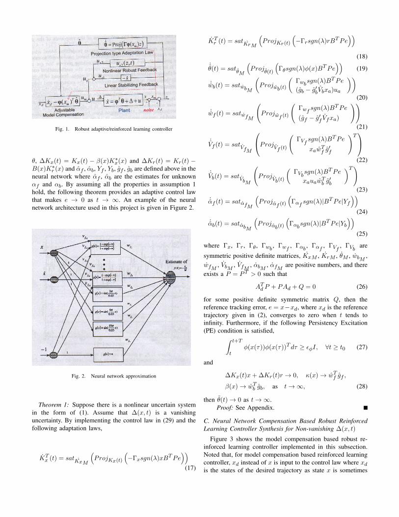
Fig. 1. Robust adaptive/reinforced learning controller

θ, ∆Kx(t) = Kx(t) − β(x)K∗x(x) and ∆Kr(t) = Kr(t) −B(x)K∗r (x) and αf , αb, Yf , Yb, gf , gb are defined above in theneural network where αf , αb are the estimates for unknownαf and αb. By assuming all the properties in assumption 1hold, the following theorem provides an adaptive control lawthat makes e → 0 as t → ∞. An example of the neuralnetwork architecture used in this project is given in Figure 2.

Fig. 2. Neural network approximation

Theorem 1: Suppose there is a nonlinear uncertain systemin the form of (1). Assume that ∆(x, t) is a vanishinguncertainty. By implementing the control law in (29) and thefollowing adaptation laws,

KTx (t) = satKxM

(ProjKx(t)

(−Γxsgn(λ)xBTPe

))(17)

KTr (t) = satKrM

(ProjKr(t)

(−Γrsgn(λ)rBTPe

))(18)

˙θ(t) = sat

θM

(Proj

θ(t)

(Γθsgn(λ)φ(x)BTPe

))(19)

˙wb(t) = satwbM

(Projwb(t)

(Γwbsgn(λ)BTPe

(gb − g′bVbxa)ua

))(20)

˙wf (t) = satwfM

(Projwf (t)

(Γwf sgn(λ)BTPe

(gf − g′f Vfxa)

))(21)

˙Vf (t) = satVfM

ProjVf (t)

(ΓVf sgn(λ)BTPe

xawTf g′f

)T(22)

˙Vb(t) = satVbM

(Proj

Vb(t)

(ΓVbsgn(λ)BTPe

xauawTb g′b

)T)(23)

˙αf (t) = satαfM

(Projαf (t)

(Γαf sgn(λ)|BTPe|Yf

))(24)

˙αb(t) = satαbM

(Projαb(t)

(Γαbsgn(λ)|BTPe|Yb

))(25)

where Γx, Γr, Γθ, Γwb , Γwf , Γαb , Γαf , ΓVf , ΓVb are

symmetric positive definite matrices, KxM , KrM , θM , wbM ,wfM , VbM , VfM , αbM , αfM are positive numbers, and thereexists a P = PT > 0 such that

ATd P + PAd +Q = 0 (26)

for some positive definite symmetric matrix Q, then thereference tracking error, e = x−xd, where xd is the referencetrajectory given in (2), converges to zero when t tends toinfinity. Furthermore, if the following Persistency Excitation(PE) condition is satisfied,∫ t+T

tφ(x(τ))φ(x(τ))T dτ ≥ εφI, ∀t ≥ t0 (27)

and

∆Kx(t)x+ ∆Kr(t)r → 0, κ(x)→ wTf gf ,

β(x)→ wTb gb, as t→∞, (28)

then θ(t)→ 0 as t→∞.Proof: See Appendix.

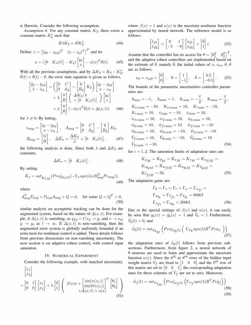
C. Neural Network Compensation Based Robust ReinforcedLearning Controller Synthesis for Non-vanishing ∆(x, t)

Figure 3 shows the model compensation based robust re-inforced learning controller implemented in this subsection.Noted that, for model compensation based reinforced learningcontroller, xd instead of x is input to the control law where xdis the states of the desired trajectory as state x is sometimes

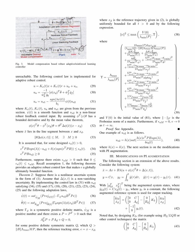
Fig. 3. Model compensation based robust adaptive/reinforced learningcontroller

unreachable. The following control law is implemented foradaptive robust control.

u = Kx(t)x+Kr(t)r + ua + us, (29)

ua =−1

wTb gb[φ(xd)T θ + wTf gf ] (30)

us = us1 −sgn(λψ(t))

b1ψ(t)us2 (31)

where Kx(t), Kr(t), ua and us1 are given from the previoussection. ψ(t) is a smooth function and us2 is a non-linearrobust feedback control input. By assuming φT (x)θ has abounded derivative and by the mean value theorem,

φ(x)T θ − φT (xd)θ = θT∆φ(x)(x− xd) (32)

where x lies in the line segment between x and xd.

‖θ∆φ(x, t)‖ ≤M, ∃ M ≥ 0 (33)

It is assumed that, for some designed εu(t) > 0,

eTPBsgn(λ)(−us2 + δ(x)sgn(eTPB)) ≤ εu(t). (34)

eTPBus2 ≥ 0 (35)

Furthermore, suppose there exists εuM > 0 such that 0 ≤εu(t) ≤ εuM . Recall assumption 1, the following theoremprovides an adaptive robust control law that makes e a globallyultimately bounded function.

Theorem 2: Suppose there is a nonlinear uncertain systemin the form of (1). Assume that ∆(x, t) is a non-vanishinguncertainty. By implementing the control law in (31) with us2satisfying (34), (35) and (17), (18), (20), (21), (22), (23), (24),(25) and the following adaptation laws,

ψ(t) = satψM

(Projψ(t)(−Γψus2BTPe)) (36)

˙θ(t) = sat

θM(Proj

θ(t)(Γθsgn(λ)φ(xd)BTPe)) (37)

where Γψ is a symmetric positive definite matrix, ψM is apositive number and there exists a P = PT > 0 such that

ATd P + PAd +Q = 0,

for some positive definite symmetric matrix Q, which Q >‖B‖ΛmaxMP , then the reference tracking error, e = x− xd,

where xd is the reference trajectory given in (2), is globallyuniformly bounded for all t > 0 and by the followingexpression.

‖e‖2 ≤ max

(V (0)

λmin(P ),Υ

), (38)

where

Υ =Λmax

λmin(P )

2λmax(P )d∞εuM(λmin(Q)−‖B‖ΛmaxMλmax(P ))

+∆Kr2

max2λmin(Γr)

+∆Kx2

max2λmin(Γx)

+4d2∞

2λmin(Γψ)+

Σmi=1(θimax−θimin)2

2λmin(Γθ)

+Σmi=1(αbimax−αbimin)2

2λmin(Γαf )

+Σmi=1(αfimax−αfimin)2

2λmin(Γalphab)

+Σmi=1(wfimax−wfimin)2

2λmin(Γwf )

+Σmi=1(wbimax−wbimin)2

2λmin(Γwb )

+‖(Vfmax−Vfmin)‖2

F2λmin(ΓVf

)

+‖(Vbmax−Vbmin)‖2

F2λmin(ΓVb

)

,

(39)

and V (0) is the initial value of (81), where ‖ · ‖F is theFrobenius norm of a matrix. Furthermore, if εuM = 0, e→ 0as t→∞.

Proof: See Appendix.One example of us2 is as follows.

us2 = h(x)sat(h(x)eTPBsgn(λ)

4ε0(t)), (40)

where h(x) = δ(x). The next section is on the modificationswith PI augmentation.

III. MODIFICATIONS ON PI AUGMENTATION

The following section is an extension of the above results.Consider the following system:

x = Ax+Bλ(u+ φ(x)T θ + ∆(x, t)),

y = Cx, yI =

∫ t

0y(τ)dτ, y(τ) = y(τ)− yc(τ). (41)

With[yTId xTd

]T being the augmented system states, whereyId(t) = Cxd(t) − yc, where yc is a constant, the followingaugmented reference system is used for output tracking.[

yIdxd

]=

([0 C0 Ad

]−[

0Bd

]K3

)[yIdxd

]+

[−10

]yc(t). (42)

Noted that, by designing K3, (for example using H2/LQR orother control techniques) the matrix([

0 C0 Ad

]−[

0Bd

]K3

)(43)

is Hurwitz. Consider the following assumption.Assumption 4: For any constant matrix K3, there exists a

constant matrix K∗3 such that

BλK3 = BK∗3 . (44)

Define: e =[(yI − yId)T (x− xd)T

]T and let

u = ([0 Kx(t)

]−K3)

[yIx

]− φ(x)T θ(t). (45)

With all the previous assumptions, and by ∆K3 = K3 −K∗3 ,θ(t) = θ(t)− θ, the error state equation is given as follows.[

yI − yIdx− xd

]=

([0 C0 Ad

]−[

0Bd

]K3

)[yI − yIdx− xd

]+ λ

[0B

](∆K3/λ+[0 Kx(t)

] ) [yIx

]+ λ

[0B

](−φ(x)T θ(t) + ∆(x, t)) (46)

for λ 6= 0. By letting,

eaug =

[yI − yIdx− xd

], Aaug =

[0 C0 Ad

]−[

0Bd

]K3,

Baug =

[0B

], ∆Kx =

∆K3

λ+[0 Kx(t)

], (47)

the following analysis is done. Since both λ and ∆K3 areconstants,

∆Kx =[0 Kx(t)

]. (48)

By setting

Kx = satKxM(ProjKx(t)(−Γxsgn(λ)xBTaugPeaug)),

(49)

where

ATaugPaug + PaugAaug +Q = 0, for some Q = QT > 0,(50)

similar analysis on asymptotic tracking can be done for theaugmented system, based on the nature of ∆(x, t). For exam-ple, if ∆(x, t) is vanishing, as yId = Cxd → yc and x→ xd,y → yc as t → ∞. If ∆(x, t) is non-vanishing, then theaugmented error system is globally uniformly bounded if anextra term for nonlinear control is added. These details followsfrom previous discussions on non-vanishing uncertainty. Thenext section is on adaptive robust control, with control inputsaturation.

IV. NUMERICAL EXPERIMENT

Consider the following example, with matched uncertainty.[x1

x2

]

=

[0 10 0

] [x1

x2

]+ λ

[01

] β(x)u+

[sin(π(x1))sin(3π(x1))

]T [θ1

θ2

]+∆(x, t) + κ(x)

(51)

where β(x) = 1 and κ(x) is the uncertain nonlinear functionapproximated by neural network. The reference model is asfollows. [

xd1xd2

]=

[0 1−5 −6

] [xd1xd2

]+

[01

]r. (52)

Assume that the controller has no access for θ =[θT1 θT2

]T ,and the adaptive robust controllers are implemented based onthe estimate of θ, namely θ, the initial values of x, xm, θ, θare as follows.

x0 = xm0 =

[00

], θ =

[1−1

], θ =

[0.5−0.5

]. (53)

The bounds of the parametric uncertainties controller param-eters are:

Λmin = −1, Λmax = 1, θimin = −π2, θimax =

π

2,

Kximin = −10, Kximax = 10, Krmin = −10,

Krmax = 10, ψmin = −10, ψmax = 10,

αfimax = 10, αfimin = 10, αbimax = 10,

αbimin = 10, wfimax = 10, wfimin = −10

wbimax = 10, wbimin = −10, wfimin = −10

Vfimax = 10, Vbimin = −10, Vbimax = 10

Vfimin = −10. (54)

for i = 1, 2. The saturation limits of adaptation rates are:

KψM = KθM = KxM = KrM = KαfiM =

KαbiM = KwfiM = KwbiM = KVbiM =

KVfiM = 50. (55)

The adaptation gains are:

Γθ = Γx = Γr = Γψ = Γwfi =

Γwbi = ΓVfi = ΓVbi = 8000I

Γαfi = Γαbi = 2000I. (56)

Due to the special settings of β(x) and κ(x), it can easilybe seen that gb(x) = gb(x) = 1 and Vb = 1 Furthermore,˙Vb(t) = 0, and

˙wb(t) = satwbM

(Projwb(t)

(Γwbsgn(λ)BTPeua

))(57)

the adaptation rates of ˙αb(t) follows from previous sub-sections. Furthermore, from figure 2, a neural network of9 neurons are used to learn and approximate the uncertainfunction κ(x). Since the 6th to 8th rows of the hidden inputweight matrix Vf are fixed to

[1 0 0

]and the 9th row of

this matrix are set to[0 0 1

], the corresponding adaptation

rates for these columns of Vf are set to zero. Moreover,

˙wf (t) = satwfM

(Projwf (t)

(Γwf sgn(λ)BTPegf

))(58)(59)

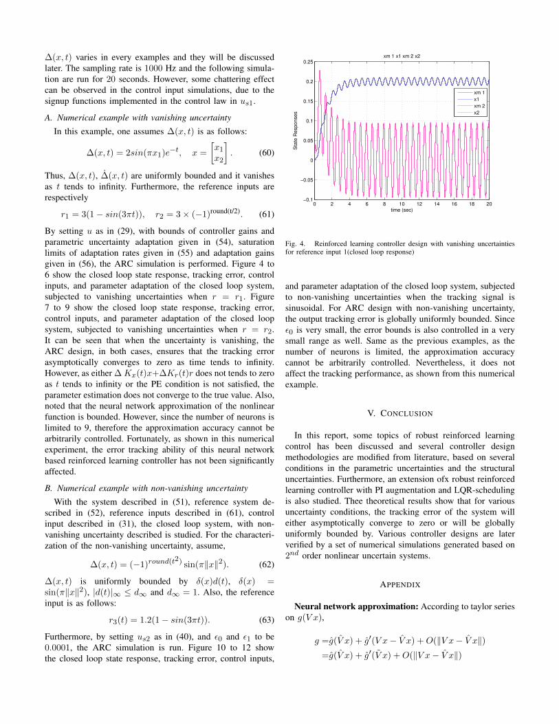
∆(x, t) varies in every examples and they will be discussedlater. The sampling rate is 1000 Hz and the following simula-tion are run for 20 seconds. However, some chattering effectcan be observed in the control input simulations, due to thesignup functions implemented in the control law in us1.

A. Numerical example with vanishing uncertainty

In this example, one assumes ∆(x, t) is as follows:

∆(x, t) = 2sin(πx1)e−t, x =

[x1

x2

]. (60)

Thus, ∆(x, t), ∆(x, t) are uniformly bounded and it vanishesas t tends to infinity. Furthermore, the reference inputs arerespectively

r1 = 3(1− sin(3πt)), r2 = 3× (−1)round(t/2). (61)

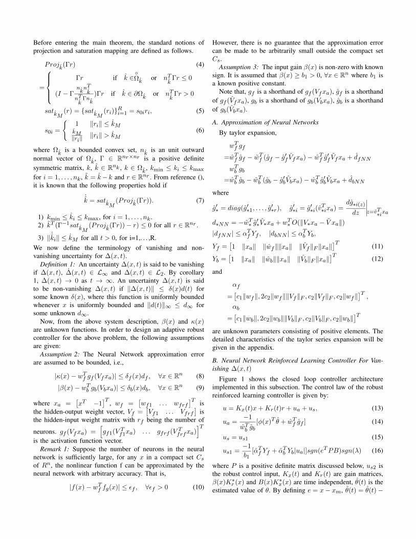
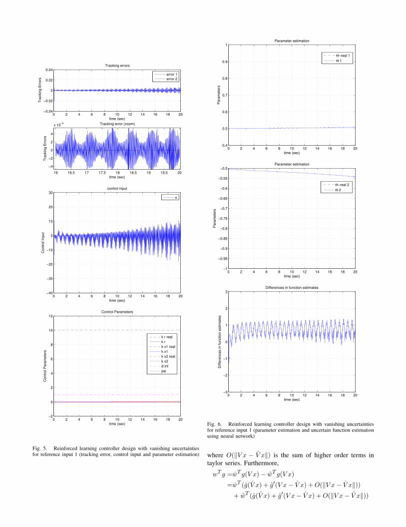
By setting u as in (29), with bounds of controller gains andparametric uncertainty adaptation given in (54), saturationlimits of adaptation rates given in (55) and adaptation gainsgiven in (56), the ARC simulation is performed. Figure 4 to6 show the closed loop state response, tracking error, controlinputs, and parameter adaptation of the closed loop system,subjected to vanishing uncertainties when r = r1. Figure7 to 9 show the closed loop state response, tracking error,control inputs, and parameter adaptation of the closed loopsystem, subjected to vanishing uncertainties when r = r2.It can be seen that when the uncertainty is vanishing, theARC design, in both cases, ensures that the tracking errorasymptotically converges to zero as time tends to infinity.However, as either ∆ Kx(t)x+∆Kr(t)r does not tends to zeroas t tends to infinity or the PE condition is not satisfied, theparameter estimation does not converge to the true value. Also,noted that the neural network approximation of the nonlinearfunction is bounded. However, since the number of neurons islimited to 9, therefore the approximation accuracy cannot bearbitrarily controlled. Fortunately, as shown in this numericalexperiment, the error tracking ability of this neural networkbased reinforced learning controller has not been significantlyaffected.

B. Numerical example with non-vanishing uncertainty

With the system described in (51), reference system de-scribed in (52), reference inputs described in (61), controlinput described in (31), the closed loop system, with non-vanishing uncertainty described is studied. For the characteri-zation of the non-vanishing uncertainty, assume,

∆(x, t) = (−1)round(t2) sin(π‖x‖2). (62)

∆(x, t) is uniformly bounded by δ(x)d(t), δ(x) =sin(π‖x‖2), |d(t)|∞ ≤ d∞ and d∞ = 1. Also, the referenceinput is as follows:

r3(t) = 1.2(1− sin(3πt)). (63)

Furthermore, by setting us2 as in (40), and ε0 and ε1 to be0.0001, the ARC simulation is run. Figure 10 to 12 showthe closed loop state response, tracking error, control inputs,

0 2 4 6 8 10 12 14 16 18 20−0.1

−0.05

0

0.05

0.1

0.15

0.2

0.25

time (sec)

Sta

te R

esp

onses

xm 1 x1 xm 2 x2

xm 1

x1

xm 2

x2

Fig. 4. Reinforced learning controller design with vanishing uncertaintiesfor reference input 1(closed loop response)

and parameter adaptation of the closed loop system, subjectedto non-vanishing uncertainties when the tracking signal issinusoidal. For ARC design with non-vanishing uncertainty,the output tracking error is globally uniformly bounded. Sinceε0 is very small, the error bounds is also controlled in a verysmall range as well. Same as the previous examples, as thenumber of neurons is limited, the approximation accuracycannot be arbitrarily controlled. Nevertheless, it does notaffect the tracking performance, as shown from this numericalexample.

V. CONCLUSION

In this report, some topics of robust reinforced learningcontrol has been discussed and several controller designmethodologies are modified from literature, based on severalconditions in the parametric uncertainties and the structuraluncertainties. Furthermore, an extension ofx robust reinforcedlearning controller with PI augmentation and LQR-schedulingis also studied. Thee theoretical results show that for variousuncertainty conditions, the tracking error of the system willeither asymptotically converge to zero or will be globallyuniformly bounded by. Various controller designs are laterverified by a set of numerical simulations generated based on2nd order nonlinear uncertain systems.

APPENDIX

Neural network approximation: According to taylor serieson g(V x),

g =g(V x) + g′(V x− V x) +O(‖V x− V x‖)=g(V x) + g′(V x) +O(‖V x− V x‖)

0 2 4 6 8 10 12 14 16 18 20−0.04

−0.02

0

0.02

0.04

time (sec)

Tra

ckin

g E

rrors

Tracking errors

error 1

error 2

16 16.5 17 17.5 18 18.5 19 19.5 20

−4

−2

0

2

4

x 10−3 Tracking error (zoom)

time (sec)

Tra

ckin

g E

rrors

0 2 4 6 8 10 12 14 16 18 20−40

−30

−20

−10

0

10

20

30

time (sec)

Co

ntr

ol In

put

control input

u

0 2 4 6 8 10 12 14 16 18 20−2

0

2

4

6

8

10

12

time (sec)

Contr

ol P

ara

mete

rs

Control Parameters

k r real

k r

k x1 real

k x1

k x2 real

k x2

d inf

psi

Fig. 5. Reinforced learning controller design with vanishing uncertaintiesfor reference input 1 (tracking error, control input and parameter estimation)

0 2 4 6 8 10 12 14 16 18 200.4

0.5

0.6

0.7

0.8

0.9

1

time (sec)

Pa

ram

ete

rs

Parameter estimation

Θ−real 1

Θ 1

0 2 4 6 8 10 12 14 16 18 20−1

−0.95

−0.9

−0.85

−0.8

−0.75

−0.7

−0.65

−0.6

−0.55

−0.5

time (sec)

Para

mete

rs

Parameter estimation

Θ−real 2

Θ 2

0 2 4 6 8 10 12 14 16 18 20−3

−2

−1

0

1

2

3

time (sec)

Diffe

rence

s in f

un

ction

estim

ate

s

Differences in function estimates

Fig. 6. Reinforced learning controller design with vanishing uncertaintiesfor reference input 1 (parameter estimation and uncertain function estimationusing neural network)

where O(‖V x − V x‖) is the sum of higher order terms intaylor series. Furthermore,

wT g =wT g(V x)− wT g(V x)

=wT (g(V x) + g′(V x− V x) +O(‖V x− V x‖))+ wT (g(V x) + g′(V x− V x) +O(‖V x− V x‖))

0 2 4 6 8 10 12 14 16 18 20−0.25

−0.2

−0.15

−0.1

−0.05

0

0.05

0.1

0.15

0.2

0.25

time (sec)

Sta

te R

esp

onses

xm 1 x1 xm 2 x2

xm 1

x1

xm 2

x2

0 2 4 6 8 10 12 14 16 18 20−0.04

−0.02

0

0.02

0.04

time (sec)

Tra

ckin

g E

rrors

Tracking errors

error 1

error 2

15.5 16 16.5 17 17.5 18 18.5 19 19.5 20−6

−4

−2

0

2

4x 10

−3 Tracking error (zoom)

time (sec)

Tra

ckin

g E

rro

rs

0 2 4 6 8 10 12 14 16 18 20−50

−40

−30

−20

−10

0

10

20

30

time (sec)

Contr

ol In

pu

t

control input

u

Fig. 7. Reinforced learning controller design with vanishing uncertaintiesfor reference input 2 (closed loop response, tracking error and control input)

wT g =wT (g − g′V x)− wT (g − g′V x)

− wT g′V x+ wTO(‖V x− V x‖)=wT (g − g′V x)− wT (g − g′V x) + dNN .

0 2 4 6 8 10 12 14 16 18 20−2

0

2

4

6

8

10

12

time (sec)

Co

ntr

ol P

ara

mete

rs

Control Parameters

k r real

k r

k x1 real

k x1

k x2 real

k x2

d inf

psi

0 2 4 6 8 10 12 14 16 18 200.4

0.5

0.6

0.7

0.8

0.9

1

time (sec)

Para

mete

rs

Parameter estimation

Θ−real 1

Θ 1

0 2 4 6 8 10 12 14 16 18 20−1

−0.95

−0.9

−0.85

−0.8

−0.75

−0.7

−0.65

−0.6

−0.55

−0.5

time (sec)

Pa

ram

ete

rs

Parameter estimation

Θ−real 2

Θ 2

Fig. 8. Reinforced learning controller design with vanishing uncertaintiesfor reference input 2 (parameter estimation)

0 2 4 6 8 10 12 14 16 18 20−3

−2

−1

0

1

2

3

time (sec)

Diffe

rences in f

unction

estim

ate

sDifferences in function estimates

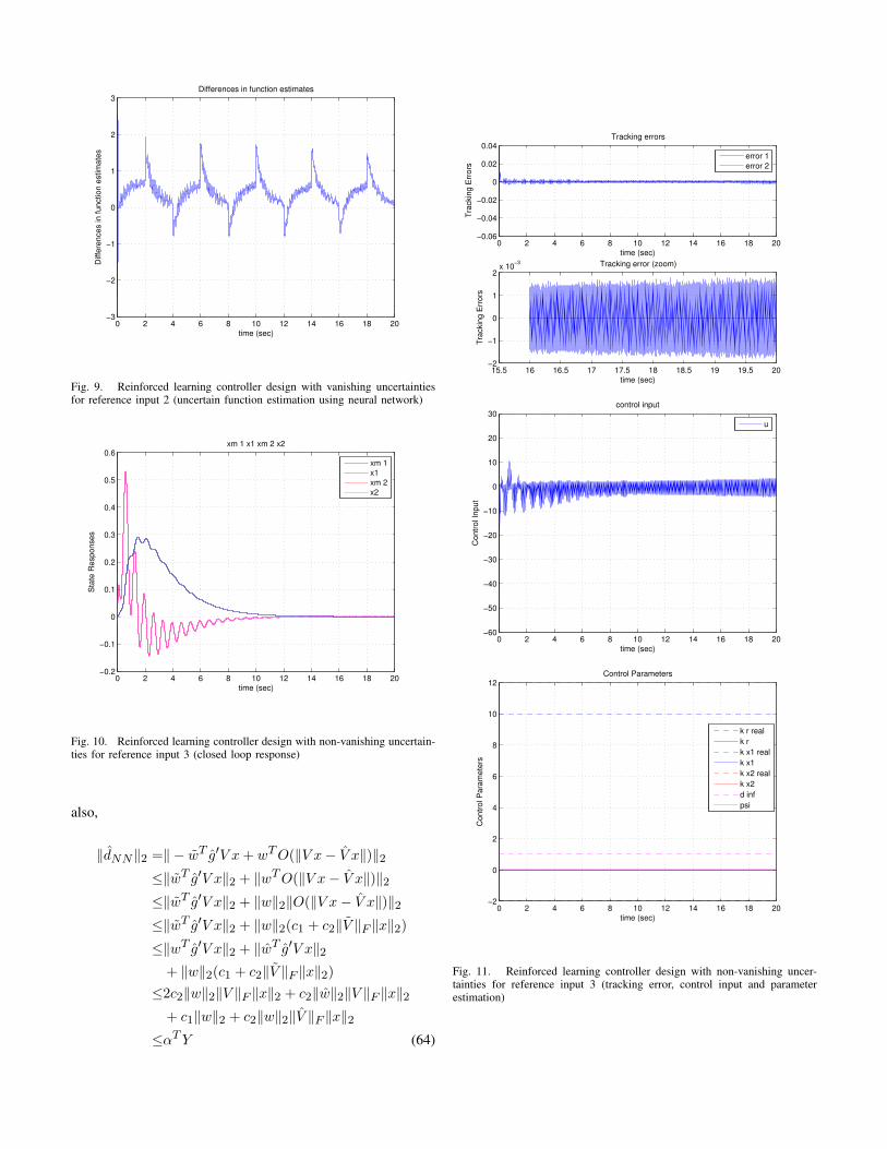
Fig. 9. Reinforced learning controller design with vanishing uncertaintiesfor reference input 2 (uncertain function estimation using neural network)

0 2 4 6 8 10 12 14 16 18 20−0.2

−0.1

0

0.1

0.2

0.3

0.4

0.5

0.6

time (sec)

Sta

te R

espo

nse

s

xm 1 x1 xm 2 x2

xm 1

x1

xm 2

x2

Fig. 10. Reinforced learning controller design with non-vanishing uncertain-ties for reference input 3 (closed loop response)

also,

‖dNN‖2 =‖ − wT g′V x+ wTO(‖V x− V x‖)‖2≤‖wT g′V x‖2 + ‖wTO(‖V x− V x‖)‖2≤‖wT g′V x‖2 + ‖w‖2‖O(‖V x− V x‖)‖2≤‖wT g′V x‖2 + ‖w‖2(c1 + c2‖V ‖F ‖x‖2)

≤‖wT g′V x‖2 + ‖wT g′V x‖2+ ‖w‖2(c1 + c2‖V ‖F ‖x‖2)

≤2c2‖w‖2‖V ‖F ‖x‖2 + c2‖w‖2‖V ‖F ‖x‖2+ c1‖w‖2 + c2‖w‖2‖V ‖F ‖x‖2

≤αTY (64)

0 2 4 6 8 10 12 14 16 18 20−0.06

−0.04

−0.02

0

0.02

0.04

time (sec)

Tra

ckin

g E

rrors

Tracking errors

error 1

error 2

15.5 16 16.5 17 17.5 18 18.5 19 19.5 20−2

−1

0

1

2x 10

−3 Tracking error (zoom)

time (sec)

Tra

ckin

g E

rrors

0 2 4 6 8 10 12 14 16 18 20−60

−50

−40

−30

−20

−10

0

10

20

30

time (sec)

Co

ntr

ol In

put

control input

u

0 2 4 6 8 10 12 14 16 18 20−2

0

2

4

6

8

10

12

time (sec)

Contr

ol P

ara

me

ters

Control Parameters

k r real

k r

k x1 real

k x1

k x2 real

k x2

d inf

psi

Fig. 11. Reinforced learning controller design with non-vanishing uncer-tainties for reference input 3 (tracking error, control input and parameterestimation)

0 2 4 6 8 10 12 14 16 18 200.4

0.5

0.6

0.7

0.8

0.9

1

time (sec)

Pa

ram

ete

rsParameter estimation

Θ−real 1

Θ 1

0 2 4 6 8 10 12 14 16 18 20−1

−0.95

−0.9

−0.85

−0.8

−0.75

−0.7

−0.65

−0.6

−0.55

−0.5

time (sec)

Para

mete

rs

Parameter estimation

Θ−real 2

Θ 2

0 2 4 6 8 10 12 14 16 18 20−4

−3

−2

−1

0

1

2

3

time (sec)

Diffe

rence

s in f

un

ction

estim

ate

s

Differences in function estimates

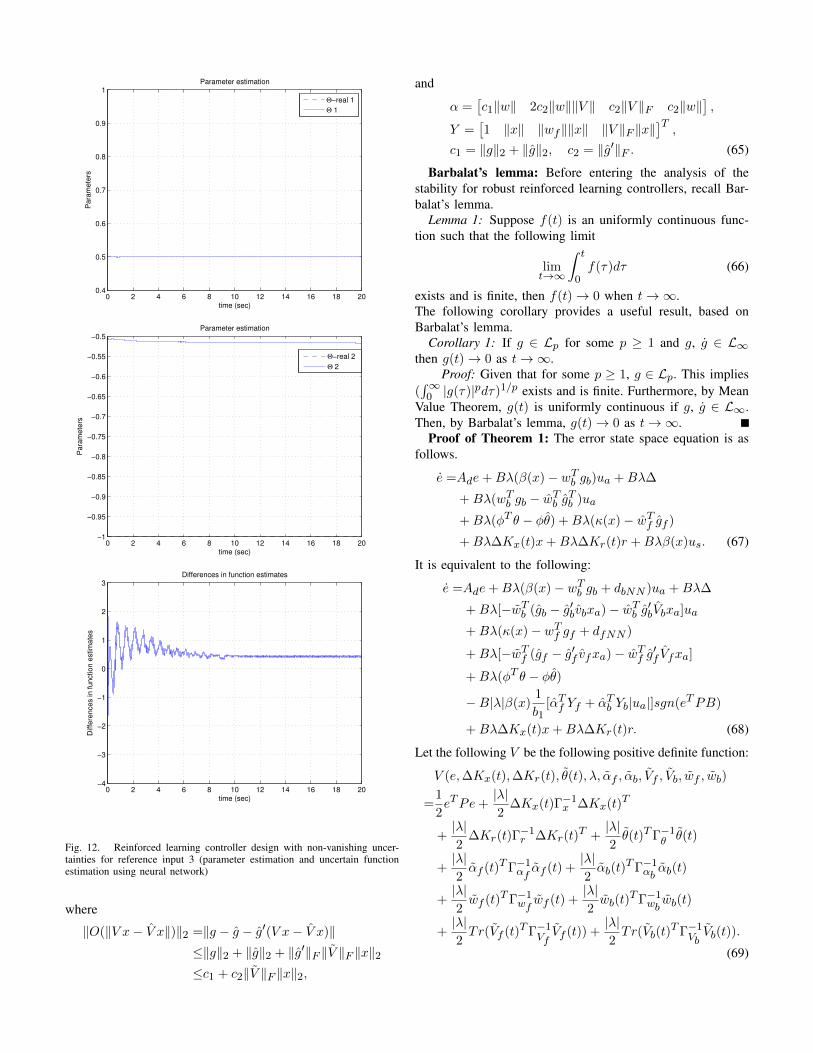
Fig. 12. Reinforced learning controller design with non-vanishing uncer-tainties for reference input 3 (parameter estimation and uncertain functionestimation using neural network)

where

‖O(‖V x− V x‖)‖2 =‖g − g − g′(V x− V x)‖≤‖g‖2 + ‖g‖2 + ‖g′‖F ‖V ‖F ‖x‖2≤c1 + c2‖V ‖F ‖x‖2,

and

α =[c1‖w‖ 2c2‖w‖‖V ‖ c2‖V ‖F c2‖w‖

],

Y =[1 ‖x‖ ‖wf‖‖x‖ ‖V ‖F ‖x‖

]T,

c1 = ‖g‖2 + ‖g‖2, c2 = ‖g′‖F . (65)

Barbalat’s lemma: Before entering the analysis of thestability for robust reinforced learning controllers, recall Bar-balat’s lemma.

Lemma 1: Suppose f(t) is an uniformly continuous func-tion such that the following limit

limt→∞

∫ t

0f(τ)dτ (66)

exists and is finite, then f(t)→ 0 when t→∞.The following corollary provides a useful result, based onBarbalat’s lemma.

Corollary 1: If g ∈ Lp for some p ≥ 1 and g, g ∈ L∞then g(t)→ 0 as t→∞.

Proof: Given that for some p ≥ 1, g ∈ Lp. This implies(∫∞0 |g(τ)|pdτ)1/p exists and is finite. Furthermore, by Mean

Value Theorem, g(t) is uniformly continuous if g, g ∈ L∞.Then, by Barbalat’s lemma, g(t)→ 0 as t→∞.

Proof of Theorem 1: The error state space equation is asfollows.

e =Ade+Bλ(β(x)− wTb gb)ua +Bλ∆

+Bλ(wTb gb − wTb g

Tb )ua

+Bλ(φT θ − φθ) +Bλ(κ(x)− wTf gf )

+Bλ∆Kx(t)x+Bλ∆Kr(t)r +Bλβ(x)us. (67)

It is equivalent to the following:

e =Ade+Bλ(β(x)− wTb gb + dbNN )ua +Bλ∆

+Bλ[−wTb (gb − g′bvbxa)− wTb g′bVbxa]ua

+Bλ(κ(x)− wTf gf + dfNN )

+Bλ[−wTf (gf − g′f vfxa)− wTf g′f Vfxa]

+Bλ(φT θ − φθ)

−B|λ|β(x)1

b1[αTf Yf + αTb Yb|ua|]sgn(eTPB)

+Bλ∆Kx(t)x+Bλ∆Kr(t)r. (68)

Let the following V be the following positive definite function:

V (e,∆Kx(t),∆Kr(t), θ(t), λ, αf , αb, Vf , Vb, wf , wb)

=1

2eTPe+

|λ|2

∆Kx(t)Γ−1x ∆Kx(t)T

+|λ|2

∆Kr(t)Γ−1r ∆Kr(t)

T +|λ|2θ(t)TΓ−1

θ θ(t)

+|λ|2αf (t)TΓ−1

αfαf (t) +

|λ|2αb(t)

TΓ−1αbαb(t)

+|λ|2wf (t)TΓ−1

wfwf (t) +

|λ|2wb(t)

TΓ−1wbwb(t)

+|λ|2Tr(Vf (t)TΓ−1

VfVf (t)) +

|λ|2Tr(Vb(t)

TΓ−1VbVb(t)).

(69)

By finding the rate of change of this function, and substitutingthe expression from (68),

V =1

2eT (ATd P + PAd)e

+ eTPBλ(β(x)− wTb gb + dbNN )ua + λeTBTP∆

+ eTPBλ(κ(x)− wTf gf + dfNN )

+ |λ|∆Kr(t)(sgn(λ)rBTPe+ Γ−1r ∆Kr(t)

T )

+ |λ|∆Kx(t)(sgn(λ)xBTPe+ Γ−1x ∆Kx(t)T )

+ |λ|θ(t)T (−sgn(λ)φBTPe+ Γ−1θ

˙θ(t)).

+ |λ|wTb

(−sgn(λ)BTPe(gb−g′bVbxa)ua + Γ−1

wb˙wb(t)

)

+ |λ|wTf

(−sgn(λ)BTPe(gf−g′f Vfxa) + Γ−1

wf˙wf (t)

)

+ |λ|Tr

[Vb(t)

TΓ−1Vb

˙Vb(t)

−VbxauawTb g′bsgn(λ)eTPB

]

+ |λ|Tr

Vf (t)TΓ−1Vf

˙Vf (t)

−VfxawTf g′fsgn(λ)eTPB

+ |λ|αTf Γ−1

f˙αf + 2|λ|αTb Γ−1

b˙αb

− |λ||eTPB|β(x)

(1

b1(αTf Yf + αTb Yb|ua|)

). (70)

Because,

|κ(x)− wTf gf | < εf , ∀εf > 0,

|β(x)− wTb gb| < εb, ∀εb > 0,

dfNN ≤ αTf Yf , dbNN ≤ αTb Yb,

and β(x)K∗r (x), β(x)K∗x(x), αb, αf , Vf , Vb, wf , wb and θ aretime independent parameters, by substituting the adaption lawsfor ˙wf (t) = ˙wf (t), ˙wb(t) = ˙wb(t)

˙θ(t) =

˙θ(t), Tr( ˙Vf (t)) =

Tr(˙Vf (t)), Tr( ˙Vb(t)) = Tr(

˙Vb(t)), ∆Kx(t)T = KT

x (t),∆Kr(t)

T = KTr (t), the above expression becomes,

V ≤1

2eT (ATd P + PAd)e+ 2λeTBTP∆

+ |eTPB||λ|αTb Yb|ua|+ |eTPB||λ|αTf Yf

− |eTPB||λ|(αTf Yf + αTb Yb|ua|)

+ |λ|αTf Γ−1f

˙αf + 2|λ|αTb Γ−1b

˙αb. (71)

By substituting the adaptation laws for ˙αf (t) = ˙αf (t),˙αb(t) = ˙αb(t),

V =1

2eT (ATd P + PAd)e+ eTPBλ∆(x, t)

≤− λmin(Q)‖e‖2 + ‖e‖‖PBλ‖‖∆(x, t)‖. (72)

From (72), with c1 equals to some arbitrary positive number,

V ≤(c21‖PB‖Λmax − λmin(Q))‖e‖2

+1

c21‖PB‖Λmax‖∆(x, t)‖2. (73)

By integrating the above expression from 0 to ∞,∫ ∞0‖e‖2dt

≤

(V (0) + Λmax

c21

∫∞0 ‖PB‖‖∆(x, t)‖2dt

)(λmin(Q)− c21‖PB‖Λmax)

. (74)

Since Q = QT > 0 is an arbitrary matrix, c1 is an arbitrarypositive constant, and Λmax is finite, if c1 is sufficiently small,there exists a Q such that λmin(Q)−c21‖PB‖Λmax > 0. Alsofrom assumption, ∆(x, t) ∈ L2. Therefore, the right hand sideof the above inequality is uniformly bounded for all t > 0 andit implies e ∈ L2. Noted that,

V (t) ≤V (0) +1

c21

∫ t

0‖PB‖Λmax‖∆(x, t)‖2dt

− (λmin(Q)− c21‖PB‖Λmax)

∫ t

0‖e‖2dt

≤V (0) +1

c21

∫ ∞0‖PB‖Λmax‖∆(x, t)‖2dt. (75)

Since the right hand side of the above inequality is uniformlybounded for all t > 0, therefore, V (t) is uniformly boundedfor any t > 0. This implies e, θ(t), ∆Kx(t) and ∆Kr(t),αf , αb, wf , wb, Vf , Vb are all uniformly bounded. Also, itis assumed that xd(t) is uniformly bounded, therefore x isalso uniformly bounded as e is uniformly bounded. ∆(x, t) isuniformly bounded for all t > 0, from (68), e is uniformlybounded. Then by corollary 1, e → 0 as r → ∞. From (2),since Ad is Hurwitz, for any uniformly bounded referenceinput r, xd(t) is uniformly bounded for all t > 0. Therefore,xd is uniformly bounded and xd(t) is uniformly continuous.Recall that e is an uniformly continuous function, x = e+xdis also uniformly continuous for all t > 0. Also, both ∆(x, t)and ∆(x, t) are uniformly bounded, ∆(x, t) is uniformlycontinuous for all t > 0. From the assumptions, θ, αb, αf , Vf ,Vb, wf , wb, B(x)K∗r (x) and B(x)K∗x(x) are bounded. Fromthe projection based adaption laws, θ(t), αf , αb, wf , wb, Vf ,Vb, Kr(t) and Kx(t) are also bounded. From the adaptationlaws, ˙

θ(t), ˙αf (t), ˙αb(t), ˙wf (t), ˙wb(t), ˙Vf (t), ˙

Wb(t), ∆Kx(t),∆Kr(t) are all bounded. Therefore, θ(t), αf , αb, wf , wb, Vf ,Vb, Kr(t) and Kx(t) are uniformly continuous. From (68),e(t) is an uniformly continuous function. With,∫ t

0e(τ)dτ = e− e(0). (76)

∫ t0 e(τ)dτ exists. By Barbalat’s lemma, e(t) → 0 as t →∞. As both e, e(t) → 0 as t → ∞. and from assumption,∆Kx(t)x+ ∆Kr(t)r → 0, κ(x)→ wTf gf , β(x)→ wTb gb ast→∞, φ(x)T θ(t)→ 0 as t→∞. For some T > 0 and as ttends to infinity,∫ t+T

tθ(t)Tφ(x(τ))φ(x(τ))T θ(t)dτ → 0. (77)

Since ˙θ(t)→ 0 as t→∞, the above expression implies,

θ(t)T

(∫ t+T

tφ(x(τ))φ(x(τ))T dτ

)θ(t)→ 0. (78)

From the PE condition, one concludes that

θ(t)T

(∫ t+T

tφ(x(τ))φ(x(τ))T dτ

)θ(t) ≥ εp‖θ(t)‖2.

(79)

As the left hand side tends to zero as t tends to infinity, θ(t)tends to zero.

Proof of Theorem 2: As in the previous theorem, the errorstate space equation is as follows.

e =Ade+Bλ(β(x)− wTb gb + dbNN )ua +Bλ∆

+Bλ[−wTb (gb − g′bvbxa)− wTb g′bVbxa]ua

+Bλ(κ(x)− wTf gf + dfNN )

+Bλ[−wTf (gf − g′f vfxa)− wTf g′f Vfxa]

+Bλ((φ(x)− φ(xd))T θ − φ(xd)T θ)

−B|λ|β(x)1

b1[αTf Yf + αTb Yb|ua|]sgn(eTPB)

+Bλ∆Kx(t)x+Bλ∆Kr(t)r +Bλβ(x)ψ(t)us2.(80)

Let V be the following positive definite function, with∆ψ(t) = ψ(t)− d∞,

V

(e,∆Kx(t),∆Kr(t), θ(t), λ, αf ,

αb, Vf , Vb, wf , wb,∆ψ(t)

)=

1

2eTPe+

|λ|2

∆Kx(t)Γ−1x ∆Kx(t)T

+|λ|2

∆Kr(t)Γ−1r ∆Kr(t)

T +|λ|2θ(t)TΓ−1

θ θ(t)

+|λ|2αf (t)TΓ−1

αfαf (t) +

|λ|2αb(t)

TΓ−1αbαb(t)

+|λ|2wf (t)TΓ−1

wfwf (t) +

|λ|2wb(t)

TΓ−1wbwb(t)

+|λ|2Tr(Vf (t)TΓ−1

VfVf (t))

+|λ|2Tr(Vb(t)

TΓ−1VbVb(t)) + |λ|Γ−1

ψ ∆ψ(t)2. (81)

By finding the rate of change of this function, and substitutingthe expression from (68) and using the adaptation laws listedin the theorem,

V ≤1

2eT (ATd P + PAd)e

+ eTPBλ(φ(x)− φ(xd))T θ

+ |λ|Γ−1ψ ∆ψ(t)∆ψ(t)

+ λeTPB

(∆(x, t)− sgn(λ)

β(x)

b1|ψ(t)|us2

). (82)

The above expression becomes,

V

≤− 1

2(λmin(Q)− ‖B‖ΛmaxMλmax(P ))‖e‖2

+ |λeTPB|δ(x)d∞ − |λ|β(x)

b1|ψ(x)|eTPBus2

+ |λ|d∞eTPBus2 − |λ|d∞eTPBus2+ |λ|Γ−1

ψ ∆ψ(t)∆ψ(t),

this becomes

V

≤− 1

2(λmin(Q)− ‖B‖ΛmaxMλmax(P ))‖e‖2

+ |λ|δψ(−eTPBus2 + Γ−1ψ ∆ψ(t)∆ψ(t))

+ |λeTPB|δ(x)d∞ − |λ|d∞eTPBus2With the adaptation law of ψ(t), the above expression be-comes,

V (83)

≤− 1

2(λmin(Q)− ‖B‖ΛmaxMλmax(P ))‖e‖2

+ |λeTPB|δ(x)d∞ − |λ|d∞eTPBus2Since ψ(t) is controlled by a projection based adaptation law,‖ψ(t)‖ ≤ d∞. If

V > λmin(P )Υ, (84)

then

(λmin(Q)− ‖B‖ΛmaxMλmax(P ))‖e‖2 > 2Λmaxd∞εuM ,(85)

it implies

V < 0. (86)

Since V is positive definite and radially unbounded, by con-trapositive argument, the tracking error is globally uniformlybounded by (38). Furthermore, by assuming r is bounded,since Ad is Hurwitz, xd(t) is globally uniformly bounded,thus x is also globally uniformly bounded. Now, if εuM = 0,the constraints in (38) vanishes and V ≤ −1

2 (λmin(Q) −‖B‖ΛmaxMλmax(P ))‖e‖2 for all e. By integration fromt = 0 to t =∞, ∫ t

0‖e(τ)‖2dτ ≤ V (0)

λmin(Q). (87)

This implies e ∈ L2. If εuM = 0, as before, e is globallyuniformly bounded. By using similar arguments as in Theorem1, one can also show that e is uniformly continuous. Therefore,by Barbalat’s lemma, e→ 0 as t→∞.

Remarks on Theorem 2: The following remarks discussessome special cases.

Remark 2: By the previous theorem, when εuM = 0, e→ 0as t→∞. The inequality (34) becomes,

eTPBsgn(λ)(−us2 + δ(x)sgn(eTPB)) ≤ 0. (88)

One way of designing us2 is by us2 =δ(x)sgn(eTPBsgn(λ)). But practically, this causes chatteringproblems.

Remark 3: Suppose Λmax is a known value and

0 ≤ εu(t) ≤ εu0(t)‖e‖+ εu1(t)d∞. (89)

where∫∞

0 εu0(τ)2dτ and∫∞

0 εu1(τ)dτ are finite. Let,

q = λmin(Q)− ‖B‖ΛmaxMλmax(P ). (90)

Recall,

V ≤− 1

2q‖e‖2

+ Λmaxd∞(εu0(t)‖e‖+ εu1(t)d∞).

Thus,

V

≤1

2Λmax

[‖e‖d∞

]T [−q/Λmax εu0(t)εu0(t) 2εu1(t)

] [‖e‖d∞

].

For some k1 > 0,[0 εu0(t)

εu0(t) 0

]≤[k2

1 00 εu0(t)2/k2

1

](91)

Thus,

V

≤1

2(∗)T

−q/Λmax

+k21

0

02εu1(t)

+εu0(t)2/k21

[‖e‖d∞].

Since k1 > 0 is a free variable, it can be arbitrarily chosensuch that (q/Λmax − k2

1) > 0. By the assumptions of εu0(t)and εu1(t), and

2V (t) ≤2V (0)− (q − k21Λmax)

∫ ∞0‖e(τ)‖2dτ

+ d2∞Λmax

∫ ∞0

2εu1(τ) + εu0(τ)2/k21dτ), (92)

it can be easily shown that e ∈ L2. Furthermore, previously ithas been shown that e, θ(t), ∆Kx(t), ∆Kr(t), ∆ψ(t), αf , αb,wf , wb, Vf , Vbare uniformly bounded. By similar proceduresas in the last theorem, x is uniformly bounded. Therefore, onecan use Barbalat’s lemma to prove that e→ 0 as t→∞. Butif the assumption of εu0(t) and εu1(t) are satisfied, εu0(t),εu1(t) → 0 as t → ∞. If e → 0 as t → ∞, this problem isthen similar to the ones in vanishing uncertainty.

REFERENCES

[1] Chad Cox, Karl Mathia, John Edwards, and Richard Akita. Modernadaptive control with neural networks. In Intertnational Conference onNeural Networks Information Processing, 1996.

[2] Lili Cui, Huaguang Zhang, Yanhong Luo, and Ning Sun. Asymptoticallystable reinforcement learning-based neural network controller usingadaptive bounding technique. In Chinese Control Conference (CCC),volume 29, pages 1582 – 1587, 2010.

[3] J. Q. Gong and B. Yao. Neural network adaptive robust control ofnonlinear systems in normal form. Asian Journal of Control, 3(2):96–110, 2001.

[4] J. Q. Gong and B. Yao. Neural network adaptive robust control ofnonlinear systems in semi-strict feedback form. Automatica, 37(8):1149–1160, 2001.

[5] J. Q. Gong and B. Yao. Neural network adaptive robust control withapplication to precision motion control of linear motors. InternationalJournal of Adaptive Control and Signal Processing, 15(8):837–864,2001.

[6] J. Q. Gong and B. Yao. Output feedback neural network adaptive robustcontrol with application to linear motor drive system. ASME Journal ofDynamic Systems, Measurement, and Control, 128(2):227–235, 2006.

[7] James Nate Knight and Charles Anderson. Stable reinforcement learningwith recurrent neural networks. Journal of Control Theory and Appli-cations, (410-420), 2011.

[8] M. Norriof. An adaptive iterative learning control algorithm withexperiments on an industrial robot. IEEE Transactions on Robotics andAutomation, 18(2):245–251, 2002.

[9] G. Santharam and S. Sastry. A reinforcement learning neural networkfor adaptive control of markov chains. In IEEE Transactions on Systems,Man, and Cybernetics, —Part A: Systems And Humans, 1997.

[10] Richard S. Sutton, Andrew G. Barto, and Ronald J. Williams. Reinforce-ment learning is direct adaptive optimal control. In American ControlConference, 1992.

[11] Draguna Vrabie, Frank L. Lewis, and Daniel S. Levine. Neural network-based adaptive optimal controller - a continuous-time formulation. ICIC,15:276–285, 2008.

[12] Xin Zhang, Huaguang Zhang, Derong Liu, and Yongsu Kim. Neural-network-based reinforcement learning controller for nonlinear systemswith non-symmetric dead-zone inputs. IEEE Transactions on Systems,Man, and Cybernetics, Part B: Cybernetics, 37(2):425 – 436, 2007.