This Page Intentionally Left Blank

i

REPORT DOCUMENTATION PAGEForm Approved

OMB No. 0704-0188

Public reporting burden for this collection of information is estimated to average 1 hour per response, including the time for reviewing instructions, searching existing data sources,gathering and maintaining the data needed, and completing and reviewing this collection of information. Send comments regarding this burden estimate or any other aspect of thiscollection of information, including suggestions for reducing this burden to Department of Defense, Washington Headquarters Services, Directorate for Information Operations andReports (0704-0188), 1215 Jefferson Davis Highway, Suite 1204, Arlington, VA 22202-4302. Respondents should be aware that notwithstanding any other provision of law, no personshall be subject to any penalty for failing to comply with a collection of information if it does not display a currently valid OMB control number. PLEASE DO NOT RETURN YOURFORM TO THE ABOVE ADDRESS.1. REPORT DATE (DD-MM-YYYY) --------- 24-04-2006 --

2. REPORT TYPEDepartment

3. DATES COVERED (From - To) 2006

4. TITLE AND SUBTITLE

NEURAL NETWORK PREDICTIONS OF THE 4-QUADRANT WAGENINGEN PROPELLER SERIES

5a. CONTRACT NUMBER

5b. GRANT NUMBER

5c. PROGRAM ELEMENT NUMBER

6. AUTHOR(S)

Robert F. Roddy, David E. Hess, and Will Faller

5d. PROJECT NUMBER

5e. TASK NUMBER

5f. WORK UNIT NUMBER

7. PERFORMING ORGANIZATION NAME(S) AND ADDRESS(ES) AND ADDRESS(ES) 8. PERFORMING ORGANIZATION REPORT NUMBER

NSWCCD-50-TR-2006/004 Naval Surface Warfare Center Carderock Division 9500 MacArthur Boulevard West Bethesda, MD 20817-5700

9. SPONSORING / MONITORING AGENCY NAME(S) AND ADDRESS(ES) 10. SPONSOR/MONITOR’S ACRONYM(S) Attn: Dr. Ronald Joslin,Code 333

Office of Naval ResearchOne Liberty Center875 N. Randolf St. Suite 1425Arlington, VA 22203-1995

11. SPONSOR/MONITOR’S REPORT NUMBER(S)

12. DISTRIBUTION / AVAILABILITY STATEMENT Approved for Public Release; Distribution Unlimited

13. SUPPLEMENTARY NOTES

14. ABSTRACTThe Maneuvering and Control Division of the Naval Surface Warfare Center (NSWC) along withApplied Simulation Technologies have been developing and applying neural networks toproblems of naval interest. This report describes the development of feedforward neuralnetwork (FFNN) predictions of four-quadrant thrust and torque behavior for the WageningenB-Screw Series of propellers and for two Wageningen ducted propeller series. The purposeof the work is twofold: to create a prediction tool that accurately recovers measured datafor those propellers in the series for which measured data is available, and to furtherprovide reasonable four-quadrant thrust and torque predictions for the remainingpropellers for which no measured data is available. Substantial results, varying each ofthe inputs over the full operating range, will be presented which establish that these twogoals have been well attained.

15. SUBJECT TERMS Hydrodynamics, Propulsors, Propellers, Four-Quadrant Prediction, 4-Quadrant Prediction, Neural Network,Feed Forward Neural Network Prediction, B-Screw Series

16. SECURITY CLASSIFICATION OF: 17. LIMITATION OF ABSTRACTSame as Report

18. NUMBEROF PAGES

78

19a. NAME OF RESPONSIBLE PERSON Robert F. Roddy

a. REPORTUnclassified

b. ABSTRACTUnclassified

c. THIS PAGEUnclassified

19b. TELEPHONE NUMBER (include areacode) 301-227-5048

Standard Form 298 (Rev. 8-98)Prescribed by ANSI Std. Z39.18

ii

This PageIntentionallyLeft Blank

iii

CONTENTS

ABSTRACT . . . . . . . . . . . . . . . . . . . . . . . . . . . . . . . . . . . . . . . . . . . . . . . . . . . . . . . . . . . . . . . . . . 1ADMINISTRATIVE INFORMATION . . . . . . . . . . . . . . . . . . . . . . . . . . . . . . . . . . . . . . . . . . . . 1INTRODUCTION . . . . . . . . . . . . . . . . . . . . . . . . . . . . . . . . . . . . . . . . . . . . . . . . . . . . . . . . . . . . . 1B-SERIES FEED FORWARD NEURAL NETWORK DEVELOPMENT . . . . . . . . . . . . . . . . . 2

METHODOLOGY . . . . . . . . . . . . . . . . . . . . . . . . . . . . . . . . . . . . . . . . . . . . . . . . . . . . . . 8DISCUSSION OF RESULTS . . . . . . . . . . . . . . . . . . . . . . . . . . . . . . . . . . . . . . . . . . . . . 12

DUCTED PROPELLER SERIES FEED FORWARD NEURAL NETWORK DEVELOPMENT . . . . . . . . . . . . . . . . . . . . . . . . . . . . . . . . . . . . . . . . . . . . . . . . . . . . . . 17METHODOLOGY . . . . . . . . . . . . . . . . . . . . . . . . . . . . . . . . . . . . . . . . . . . . . . . . . . . . . 18DISCUSSION OF RESULTS . . . . . . . . . . . . . . . . . . . . . . . . . . . . . . . . . . . . . . . . . . . . . 18

UTILIZATION OF THE FFNNs FOR THE B-SCREW SERIES AND TWO DUCTED PROPELLER SERIES . . . . . . . . . . . . . . . . . . . . . . . . . . . . . . . . . . . . . . . . . . . . . . . . 19CONCLUSIONS AND RECOMMENDATIONS . . . . . . . . . . . . . . . . . . . . . . . . . . . . . . . . . . . 22REFERENCES . . . . . . . . . . . . . . . . . . . . . . . . . . . . . . . . . . . . . . . . . . . . . . . . . . . . . . . . . . . . . . 23APPENDIX A - Summary of Coefficients and Results From “Recent Developments in

Marine Propeller Hydrodynamics” (Reference 14) . . . . . . . . . . . . . . . . A1APPENDIX B - Summary of Coefficients and Results From “Vier_Kwadrant Vrijvarende-

Schroef-Karakterstieken Voor B-Serie Schroeven. Fourier-Reeks Ontwikkeling en Operationeel Gebruik”(Reference 15) . . . . . . . . . . . . B1APPENDIX C - Intelligent Calculation of Equations (ICE) . . . . . . . . . . . . . . . . . . . . . . . . . . . C1APPENDIX D - Derivation of Matching Polynomial Computation . . . . . . . . . . . . . . . . . . . . . D1

Matching Polynomial Computation . . . . . . . . . . . . . . . . . . . . . . . . . . . . . . . . . . . . . . . . D2Matching Curvatures . . . . . . . . . . . . . . . . . . . . . . . . . . . . . . . . . . . . . . . . . . . . . . . . . . . D4

APPENDIX E -Summary of Coefficients and Results For Nozzle 19a with Ka4-70 From “Wake Adapted Ducted Propellers” (Reference 16) . . . . . . . . . . . . . . . . . . . . . . E1

APPENDIX F -Summary of Coefficients and Results For Nozzle 37 with Ka4-70 From “Wake Adapted Ducted Propellers” (Reference 16) . . . . . . . . . . . . . . . . . . . . . . F1

iv

FIGURES

1 Characteristics of B4-Series of Propellers . . . . . . . . . . . . . . . . . . . . . . . . . . . . . . . . . . . . . 22 B4-70 Series of Open Water Curves from Regression Analysis Coefficients . . . . . . . . . . 23 B4-70 Series 4-Quadrant Results . . . . . . . . . . . . . . . . . . . . . . . . . . . . . . . . . . . . . . . . . . . . 54 Definition of the Average Angle Measure . . . . . . . . . . . . . . . . . . . . . . . . . . . . . . . . . . . . . 75 Example of Blending an Open-Water Curve and 4-Quadrant Data . . . . . . . . . . . . . . . . . 86 Sample of CT* Training Results over Entire $ Range with SIN and COS Terms . . . . . . . 97 Sample of CT* of Initial Training Results with the $ Range Subdivided into

Four Regions . . . . . . . . . . . . . . . . . . . . . . . . . . . . . . . . . . . . . . . . . . . . . . . . . . . . . . . . . . 108 Ranges for ICE Training . . . . . . . . . . . . . . . . . . . . . . . . . . . . . . . . . . . . . . . . . . . . . . . . . 119 Four Quadrant Prediction for B3-EAR (P/D=1.0) Propeller Series Showing

Comparison with Measured Data; Symbols = Measured Data, Solid Lines = Predictions . . . . . . . . . . . . . . . . . . . . . . . . . 13

10 Four Quadrant Prediction for B6-EAR (P/D=1.0) Propeller Series Showing Comparison with Measured Data; Symbols = Measured Data, Solid Lines = Predictions . . . . . . . . . . . . . . . . . . . . . . . . . 13

11 4-Quadrant Predictions for a B5-40, B5-60, and B5-100 Series . . . . . . . . . . . . . . . . . . . 1412 4-Quadrant Predictions for BZ-40, BZ-65, and BZ-100 Series with P/D=1.0 . . . . . . . . 1513 4-Quadrant Predictions for B5-EAR (P/D = 0.6, 1.0, 1.4) Series . . . . . . . . . . . . . . . . . . 1614 Profiles on MARIN Nozzles 19a and 37 . . . . . . . . . . . . . . . . . . . . . . . . . . . . . . . . . . . . . 1715 Profile of Ka4-70 Series of Propellers . . . . . . . . . . . . . . . . . . . . . . . . . . . . . . . . . . . . . . . 1716 Four Quadrant Prediction for Nozzle 19a with Ka4-70 Propeller Series

Symbols = Measured Data, Solid Lines = Predictions . . . . . . . . . . . . . . . . . . . . . . . . . 1817 Four Quadrant Prediction for Nozzle 37 with Ka4-70 Propeller Series

Symbols = Measured Data, Solid Lines = Predictions . . . . . . . . . . . . . . . . . . . . . . . . . 19A1 B4-70 Series of Open-Water Curves from Regression Analysis Coefficients . . . . . . A-4B1 B4-70 Series 4-Quadrant Results . . . . . . . . . . . . . . . . . . . . . . . . . . . . . . . . . . . . . . . . . B-17B2 B4-EAR Series (P/D = 1.0) 4-Quadrant Results . . . . . . . . . . . . . . . . . . . . . . . . . . . . . B-17B3 B-(Blade No.) Series (P/D = 1.0 and EAR . 0.7) . . . . . . . . . . . . . . . . . . . . . . . . . . . . B-18D1 Plot of Thrust Coefficient Vs. Beta Showing Mismatched Predictions at

One of the Boundaries . . . . . . . . . . . . . . . . . . . . . . . . . . . . . . . . . . . . . . . . . . . . . . . . . D-2D2 Plot of Thrust Coefficient vs. Beta Showing Matching Polynomials Computed

Using Both Methods . . . . . . . . . . . . . . . . . . . . . . . . . . . . . . . . . . . . . . . . . . . . . . . . . . D-5E1 Nozzle 19a with Ka4-70 4-Quadrant Results . . . . . . . . . . . . . . . . . . . . . . . . . . . . . . . . E-6F1 Nozzle 37 with Ka4-70 4-Quadrant Results . . . . . . . . . . . . . . . . . . . . . . . . . . . . . . . . . F-6

v

TABLES

1 Summary of B-Screw Series Propellers . . . . . . . . . . . . . . . . . . . . . . . . . . . . . . . . . . . . . . . 12 Quadrant Definitions for the J, KT, and KQ Coordinate System . . . . . . . . . . . . . . . . . . . . 43 Quadrant Definitions for the $, CT*, and CQ

* Coordinate System . . . . . . . . . . . . . . . . . . . 44 Summary of B-Screw Series Propellers with 4-Quadrant Test Results

[P/Ds for Propellers tested are shown] . . . . . . . . . . . . . . . . . . . . . . . . . . . . . . . . . . . . . . . 55 Initial Regions for Subdivided Data . . . . . . . . . . . . . . . . . . . . . . . . . . . . . . . . . . . . . . . . 106 Boundaries and Ranges for ICE Training . . . . . . . . . . . . . . . . . . . . . . . . . . . . . . . . . . . . 117 Sample of a Single Propeller Prediction Run . . . . . . . . . . . . . . . . . . . . . . . . . . . . . . . . . 208 Sample of a Prediction Run for a Family of Propellers . . . . . . . . . . . . . . . . . . . . . . . . . . 21A1 Coefficients and Terms of the KT and KQ Polynomials for the B-Screw Series . . . . . A-3B1 Propellers for Which MARIN has 4-Quadrant Results . . . . . . . . . . . . . . . . . . . . . . . . . B-2B2 Coefficients for B4-100, P/D = 1.0 . . . . . . . . . . . . . . . . . . . . . . . . . . . . . . . . . . . . . . . . B-3B3 Coefficients for B4-85, P/D = 1.0 . . . . . . . . . . . . . . . . . . . . . . . . . . . . . . . . . . . . . . . . . B-4B4 Coefficients for B4-70, P/D = 1.0 . . . . . . . . . . . . . . . . . . . . . . . . . . . . . . . . . . . . . . . . . B-5B5 Coefficients for B4-55, P/D = 1.0 . . . . . . . . . . . . . . . . . . . . . . . . . . . . . . . . . . . . . . . . . B-6B6 Coefficients for B4-40, P/D = 1.0 . . . . . . . . . . . . . . . . . . . . . . . . . . . . . . . . . . . . . . . . . B-7B7 Coefficients for B3-65, P/D = 1.0 . . . . . . . . . . . . . . . . . . . . . . . . . . . . . . . . . . . . . . . . . B-8B8 Coefficients for B5-75, P/D = 1.0 . . . . . . . . . . . . . . . . . . . . . . . . . . . . . . . . . . . . . . . . . B-9B9 Coefficients for B6-80, P/D = 1.0 . . . . . . . . . . . . . . . . . . . . . . . . . . . . . . . . . . . . . . . . B-10B10 Coefficients for B7-85, P/D = 1.0 . . . . . . . . . . . . . . . . . . . . . . . . . . . . . . . . . . . . . . . . B-11B11 Coefficients for B4-70, P/D = 0.5 . . . . . . . . . . . . . . . . . . . . . . . . . . . . . . . . . . . . . . . . B-12B12 Coefficients for B4-70, P/D = 0.6 . . . . . . . . . . . . . . . . . . . . . . . . . . . . . . . . . . . . . . . . B-13B13 Coefficients for B4-70, P/D = 0.8 . . . . . . . . . . . . . . . . . . . . . . . . . . . . . . . . . . . . . . . . B-14B14 Coefficients for B4-70, P/D = 1.2 . . . . . . . . . . . . . . . . . . . . . . . . . . . . . . . . . . . . . . . . B-15B15 Coefficients for B4-70, P/D = 1.4 . . . . . . . . . . . . . . . . . . . . . . . . . . . . . . . . . . . . . . . . B-16E1 Coefficients for Nozzle 19a with Ka4-70 . . . . . . . . . . . . . . . . . . . . . . . . . . . . . . . . . . . E-3F1 Coefficients for Nozzle 37 with Ka4-70 . . . . . . . . . . . . . . . . . . . . . . . . . . . . . . . . . . . . F-3

vi

Nomenclature

AAM Average Angle MeasureAE Expanded Blade Area of PropellerAO Disk Area of PropellerC0.7R Chord Length of Propeller Blade Section at the 70% RadiusCQ

* Torque Coefficient, CQ* = Q/{½ρ[ Va

2+(0.7πnD)2](π/4)D3}CTn

* Thrust Coefficient due to the Duct, CTn* = Tn/{½ρ[ Va

2+(0.7πnD)2](π/4)D2}CT

* Thrust Coefficient, or Total Thrust Coefficient of Ducted Propeller System, CT

* = T/{½ρ[ Va2+(0.7πnD)2](π/4)D2}

D Propeller DiameterETA Open-Water Efficiency = ηoJ Advance Coefficient, J = VA/(nD)KT Thrust Coefficient, or Total Thrust Coefficient of Ducted Propeller System,

KT = T/(ρn2D4)KTn Thrust Coefficient due to the Duct, KTn = Tn/(ρn2D4)KQ Torque Coefficient, KQ = Q/(ρn2D5)N Number of Revolutions per Minuten Number of Revolutions per SecondQ TorqueP Propeller Blade Pitchr Correlation CoefficientR Propeller RadiusRn0.7R Reynolds Number based on the Chord Length of the Propeller Blade Section

at the 70% Radius, Rn0.7R = { C0.7R[Va2 + (0.7πnD)2]1/2}/ν

RPM Number of Revolutions per MinuteT Thrust, Total Thrust of a Ducted Propeller SystemTn Thrust of the Duct in a Ducted Propeller SystemVa Undisturbed Stream VelocityZ Number of Propeller Blades

EAR Expanded, or Blade, Area Ratio of Propeller, EAR = AE/ AOP/D Pitch to Diameter Ratio of Propeller

β Advance Angle at the 70% Radius, β = arctan (Va/(0.7πnD))ηo Open-Water Efficiency, ηo = (J KT)/(2π KQ) = (0.7CT

*tan(β))/(2CQ*)

ρ Density of Waterν Kinematic Viscosity of Water

1

ABSTRACT

The Maneuvering and Control Division at the David Taylor Model Basin, Naval Surface Warfare Center (NSWC) along with Applied Simulation Technologies have been developing and applying neural networks to problems of naval interest. This report describes the development of feedforward neural network (FFNN) predictions of four-quadrant thrust and torque behavior for the Wageningen B-Screw Series of propellers and for two Wageningen ducted propeller series. The purpose of the work is twofold: to create a prediction tool that accurately recovers measured data for those propellers in the series for which measured data is available, and to further provide reasonable four-quadrant thrust and torque predictions for the remaining propellers for which no measured data is available. Substantial results, varying each of the inputs over the full operating range, will be presented which establish that these two goals have been well attained.

ADMINISTRATIVE INFORMATION

This work was supported by the Office of Naval Research and by NSWCCD.

INTRODUCTION

During preliminary ship design studies an estimate of the performance of the proposed propeller is required. One of the most used subcavitating open-propeller series is the Wageningen B-Screw Series. Experimental data on the series was first reported in 19371. As additional propellers were added to the series, and new techniques were developed, additional reports on the series were issued from 1937 to 19842-15. The parameters that were varied in this series are: the number of propeller blades (Z); the expanded area ratio of the propellers (EAR); and, the pitch-diameter ratio of the propellers (P/D). The B-Series propellers are defined as Bm-nn, where m=Z and nn=EAR*100. Table 1 presents a summary of the principal geometric characteristics of the propellers contained within the B-Screw Series while Figure 1 shows the characteristics of the B4-Series of propellers reproduced from Reference 10. The information in these references is sufficient for performing preliminary powering estimates; however, to conduct ship performance simulations, this information must be supplemented with four-quadrant thrust and torque performance of the desired propeller.

For ducted propeller estimates, similar information was published by Oosterveld16. A

very good summary of all of the MARIN propeller series results is presented in “The Wageningen Propeller Series”17. The discussion of the development of the FFNNs is divided into two sections. The first section discusses the B-Series FFNN development and the second section discusses the developments for the ducted propeller FFNNs. Table 1 – Summary of B-Screw Series Propellers

Z\EAR 0.30 0.35 0.38 0.40 0.45 0.50 0.55 0.60 0.65 0.70 0.75 0.80 0.85 0.90 0.95 1.00 1.05 P/D Ranges2 X X 0.6 - 1.43 X X X X X B3-35 [0.6 - 1.4]; Remainder [0.5 - 1.4]4 X X X X X 0.5 - 1.45 X X X X 0.5 - 1.46 X X X 0.5 - 1.47 X X X X 0.5 - 1.4

2

Figure 1 – Characteristics of the B4-Series of Propellers

B-SERIES FEED FORWARD NEURAL NETWORK DEVELOPMENT In Reference 14, “Recent Developments in Marine Propeller Hydrodynamics”,

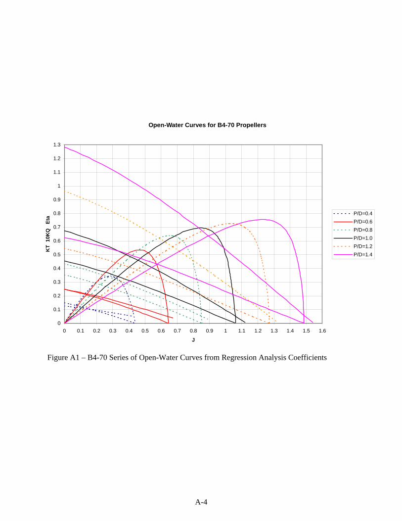
regression analysis coefficients are presented that allow a user to accurately compute the thrust and torque performance characteristics of any propeller within the series to produce standard open water curves using the usual J, KT, 10KQ nomenclature. (Note: Open Water curves present data that is in the first part of the first quadrant of 4-quadrant data.) With these coefficients it is a straightforward procedure to computerize the process of: optimization of propeller diameter or RPM; estimation of the open water performance of the optimized propeller; estimating the off-design performance of the optimized propeller; and, performing design trade-off studies. Presented in Appendix A are the regression analysis coefficients determined in Reference 14. A sample plot of results using these coefficients is shown in Figure 2. Figure 2 – B4-70 Series of Open-Water Curves from Regression Analysis Coefficients

Open-Water Curves for B4-70 Propellers

0

0.1

0.2

0.3

0.4

0.5

0.6

0.7

0.8

0.9

1

1.1

1.2

1.3

0 0.1 0.2 0.3 0.4 0.5 0.6 0.7 0.8 0.9 1 1.1 1.2 1.3 1.4 1.5 1.6

J

KT

10K

Q

Eta

P/D=0.4P/D=0.6P/D=0.8P/D=1.0P/D=1.2P/D=1.4

Solid Lines: KT and Eta Dashed Lines: 10KQ

3

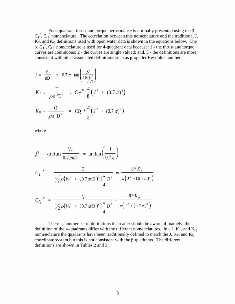
Four-quadrant thrust and torque performance is normally presented using the β, CT

*, CQ* nomenclature. The correlation between this nomenclature and the traditional J,

KT, and KQ definitions used with open water data is shown in the equations below. The β, CT

*, CQ* nomenclature is used for 4-quadrant data because: 1 - the thrust and torque

curves are continuous; 2 - the curves are single valued; and, 3 - the definitions are more consistent with other associated definitions such as propeller Reynolds number.

where

There is another set of definitions the reader should be aware of; namely, the definition of the 4-quadrants differ with the different nomenclatures. In a J, KT, and KQ nomenclature the quadrants have been traditionally defined to match the J, KT, and KQ coordinate system but this is not consistent with the β quadrants. The different definitions are shown in Tables 2 and 3.

J =⎛

⎝⎜⎜

⎞

⎠⎟⎟

VnD

= 0.7 tan 180a

πβ

π

( )K JT = 2 4 = 2T

n D CT*8

+ (0.7ρ

ππ2 )

( )K JQ = 2 5

2Q n D = CQ *

8 + (0.7

ρπ

π2 )

βπ π

= arctan V

nDJa

0 7 0 7.arctan

.=

⎛⎝⎜

⎞⎠⎟

( ){ } ( )( )CT

T

V D

K

Ja

T* *

. =

+ 0.7 nD12

4

8

0 72 2 2 2 2ρ ππ π π

=+

( ){ } ( )( )CQ

Q

V D

K

Ja

Q* *

. =

+ 0.7 nD12

4

8

0 72 2 3 2 2ρ ππ π π

=+

4

Table 2 – Quadrant Definitions for the J, KT, and KQ Coordinate System

Quadrant Number

Quadrant Description Beta (β) [deg]

1 Ahead 0 - 902 Crashahead 270 - 360 3 Crashback 90 - 180 4 Backing 180 - 270

Table 3 – Quadrant Definitions for the β, CT

*, CQ* Coordinate System

Quadrant Number

Quadrant Description Beta (β) [deg]

1 Ahead 0 - 902 Crashback 90 - 180 3 Backing 180 - 270 4 Crashahead 270 - 360

Since the β nomenclature does not use the J, KT, and KQ nomenclature, it is not bound to the older quadrant definitions defined by J, KT, and KQ. The quadrant definitions used with the β, CT

*, CQ* nomenclature follows the hydrodynamic angle-of-

attack of the propeller blades. The β, CT*, CQ

* nomenclature has more consistency with propeller physics than the older quadrant definition used with the J, KT, and KQ nomenclature. Reference 15 presents harmonic analysis coefficients that enable the computation of the 4-quadrant thrust and torque performance for a subset of the B-Screw Series using the β, CT

*, CQ* nomenclature. Table 4 presents the geometric propeller characteristics of

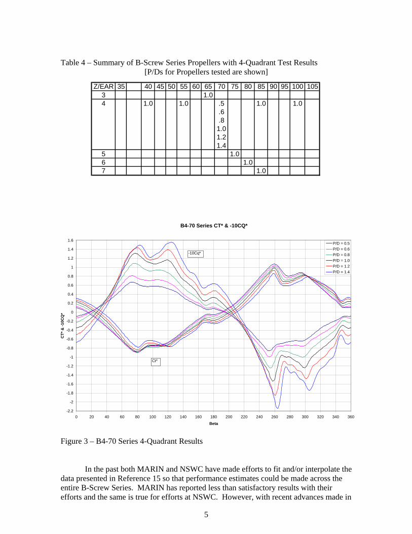
this subset. An examination of Table 4 reveals that this subset of the B-Screw Series contains three parameter sweeps: 1 – a sweep across the range of P/D’s for B4-70 propellers; a sweep across the range of EARs for a series of 4-bladed propellers with a P/D=1.00; and, a sweep across the range of propeller blade numbers for a series of propellers with a P/D=1.00 and an EAR≈0.7. Presented in Appendix B are the harmonic analysis coefficients determined in Reference 15 and some sample plots of results using these coefficients. One sample plot of the results using these coefficients is shown in Figure 3.

5

Table 4 – Summary of B-Screw Series Propellers with 4-Quadrant Test Results

[P/Ds for Propellers tested are shown]

Figure 3 – B4-70 Series 4-Quadrant Results In the past both MARIN and NSWC have made efforts to fit and/or interpolate the data presented in Reference 15 so that performance estimates could be made across the entire B-Screw Series. MARIN has reported less than satisfactory results with their efforts and the same is true for efforts at NSWC. However, with recent advances made in

Z/EAR 35 40 45 50 55 60 65 70 75 80 85 90 95 100 1053 1.04 1.0 1.0 .5

.6

.8 1.0 1.2 1.4

1.0 1.0

5 1.06 1.07 1.0

B4-70 Series CT* & -10CQ*

-2.2

-2

-1.8

-1.6

-1.4

-1.2

-1

-0.8

-0.6

-0.4

-0.2

0

0.2

0.4

0.6

0.8

1

1.2

1.4

1.6

0 20 40 60 80 100 120 140 160 180 200 220 240 260 280 300 320 340 360

Beta

CT*

& -1

0CQ

*

P/D = 0.5P/D = 0.6P/D = 0.8P/D = 1.0P/D = 1.2P/D = 1.4

-10Cq*

Ct*

6

using Feedforward Neural Networks (FFNN), a successful effort was made to train a neural network using a combination of the data obtained from References 14 and 15. This section of the report describes the approach used and the results obtained using FFNN to estimate the 4-quadrant thrust and torque performance of the B-Screw Series.

A FFNN is a computational technique for developing nonlinear equation systems that relate input variables to output variables. In a feedforward network information travels from input nodes through internal groupings of nodes (hidden layers) to the output nodes. A FFNN is distinguished from a recursive neural network (RNN) by the fact that the latter employs feedback; namely, the information stream issuing from the outputs is redirected to form additional inputs to the network. The additional complexity of an RNN is required for the solution of difficult time-dependent problems such as the simulation of the motion of a maneuvering submarine18, or surface ship19.

Feedforward neural networks, on the other hand, are employed for a wide array of

uses. Correctly trained FFNNs offer two primary functions: first, they serve as an efficient means for accurately recovering an experimental data set long after the experiment has concluded, and second, they have the ability to predict data that was not measured but is similar to the training data.

The FFNNs used here are fully connected with two hidden layers and use 0 to 1

sigmoid activation functions trained by backpropagation. Each FFNN typically has a single output to maximize prediction quality; therefore, problems with more than one dependent variable use multiple networks. The available experimental or numerical data is partitioned into two sets: training data (80%) used to train the network and adjust the weights via backpropagation, and validation data (20%) used along with the training data to test the performance of the trained network. Prediction quality is judged by two error measures: the average angle measure (AAM) described below, and a correlation coefficient (r). For both measures, a numerical value of one indicates perfect agreement between measured data and predictions, whereas a value of zero denotes no agreement.

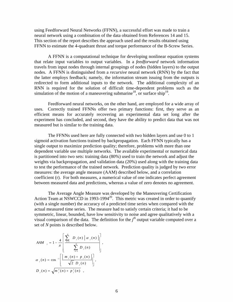
The Average Angle Measure was developed by the Maneuvering Certification Action Team at NSWCCD in 1993-199420. This metric was created in order to quantify (with a single number) the accuracy of a predicted time series when compared with the actual measured time series. The measure had to satisfy certain criteria; it had to be symmetric, linear, bounded, have low sensitivity to noise and agree qualitatively with a visual comparison of the data. The definition for the jth output variable computed over a set of N points is described below.

, )()()(

, )(2

)()(cos)(

, )(

)()(41

22

1

1

1

npnmnD

nD

npnmn

nD

nnDAAM

jjj

j

jj

j

N

nj

N

njj

j

+=

⎥⎥⎦

⎤

⎢⎢⎣

⎡ +=

⎥⎥⎥⎥

⎦

⎤

⎢⎢⎢⎢

⎣

⎡

−=

−

=

=

∑

∑

α

α

π

7

Given a predicted value, p, and an experimentally measured value, s, one can plot a point in p-s space as shown in Fig. 4. Figure 4 - Definition of the Average Angle Measure

If the prediction is perfect, then the point will fall on a 45° line extended from the origin; the distance from the origin will depend upon the magnitude of s. If sp ≠ , the point will fall on one side or the other of the 45° line. If one extends a line from the origin such that it passes through this point, one can consider the angle between this new line and the 45° line, measured from the 45° line. This angle is a measure of the error of the prediction. To extend this error metric to a set of N points, one computes the average angle of the set. A problem arises, however. When s is small and p is relatively close to s, one may still obtain a comparatively large angle. On the other hand, when s is large and p is relatively far from s, one may obtain a relatively small angle. To correct this, the averaging process is weighted by the distance of each point from the origin. The statistic is then normalized to give a value between –1 and 1. A value of 1 corresponds to perfect magnitude and phase correlation, -1 implies perfect magnitude correlation but 180° out of phase and zero indicates no magnitude or phase correlation. This metric is not perfect; it gives a questionable response for maneuvers with flat responses, predictions with small constant offsets and small magnitude signals. Nevertheless, it is in most cases an excellent quantitative measure of agreement. The FFNN is developed using executable code that automates the process of solving nonlinear equation systems. The code, “Intelligent Calculation of Equations” (ICE), was developed by Applied Simulation Technologies and is available without charge. The ICE routines work on two user defined input data sets. One data set is comprised of independent variables (inputs) and dependent variables (outputs). There can be as many as 10,000 input data points and the only restriction is that the data be in ASCII columnar format. The second input data set specifies the options the user desires for the training. These options make ICE a powerful and versatile tool. A more complete description of ICE is presented in Appendix C.

8

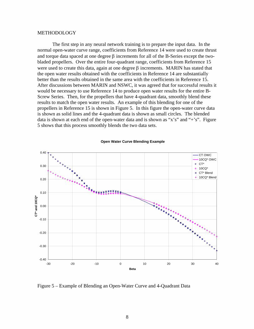
METHODOLOGY The first step in any neural network training is to prepare the input data. In the normal open-water curve range, coefficients from Reference 14 were used to create thrust and torque data spaced at one degree β increments for all of the B-Series except the two-bladed propellers. Over the entire four-quadrant range, coefficients from Reference 15 were used to create this data, again at one degree β increments. MARIN has stated that the open water results obtained with the coefficients in Reference 14 are substantially better than the results obtained in the same area with the coefficients in Reference 15. After discussions between MARIN and NSWC, it was agreed that for successful results it would be necessary to use Reference 14 to produce open water results for the entire B-Screw Series. Then, for the propellers that have 4-quadrant data, smoothly blend these results to match the open water results. An example of this blending for one of the propellers in Reference 15 is shown in Figure 5. In this figure the open-water curve data is shown as solid lines and the 4-quadrant data is shown as small circles. The blended data is shown at each end of the open-water data and is shown as “x’s” and “+’s”. Figure 5 shows that this process smoothly blends the two data sets. Figure 5 – Example of Blending an Open-Water Curve and 4-Quadrant Data

Open Water Curve Blending Example

-0.40

-0.30

-0.20

-0.10

0.00

0.10

0.20

0.30

0.40

-30 -20 -10 0 10 20 30 40

Beta

CT*

and

10C

Q*

CT OWC10CQ* OWCCT*10CQ*CT* Blend10CQ* Blend

9

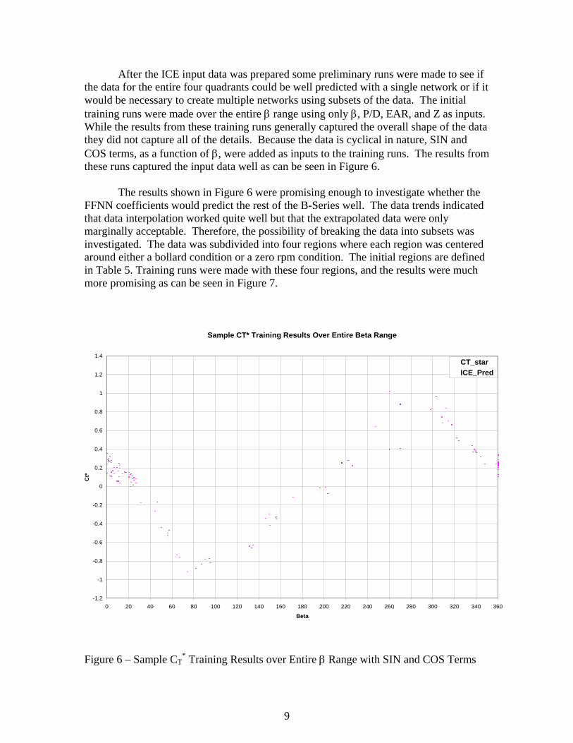
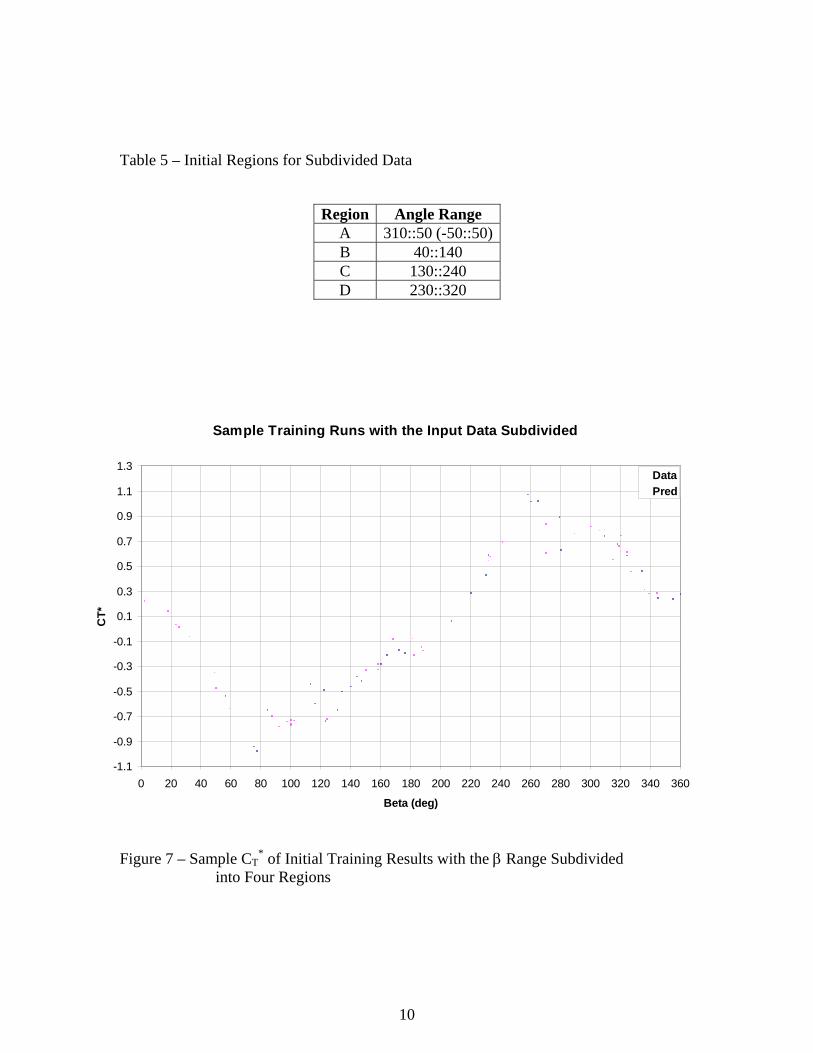
After the ICE input data was prepared some preliminary runs were made to see if the data for the entire four quadrants could be well predicted with a single network or if it would be necessary to create multiple networks using subsets of the data. The initial training runs were made over the entire β range using only β, P/D, EAR, and Z as inputs. While the results from these training runs generally captured the overall shape of the data they did not capture all of the details. Because the data is cyclical in nature, SIN and COS terms, as a function of β, were added as inputs to the training runs. The results from these runs captured the input data well as can be seen in Figure 6. The results shown in Figure 6 were promising enough to investigate whether the FFNN coefficients would predict the rest of the B-Series well. The data trends indicated that data interpolation worked quite well but that the extrapolated data were only marginally acceptable. Therefore, the possibility of breaking the data into subsets was investigated. The data was subdivided into four regions where each region was centered around either a bollard condition or a zero rpm condition. The initial regions are defined in Table 5. Training runs were made with these four regions, and the results were much more promising as can be seen in Figure 7. Figure 6 – Sample CT

* Training Results over Entire β Range with SIN and COS Terms

Sample CT* Training Results Over Entire Beta Range

-1.2

-1

-0.8

-0.6

-0.4

-0.2

0

0.2

0.4

0.6

0.8

1

1.2

1.4

0 20 40 60 80 100 120 140 160 180 200 220 240 260 280 300 320 340 360

Beta

Ct*

CT_starICE_Pred

10

Table 5 – Initial Regions for Subdivided Data Figure 7 – Sample CT

* of Initial Training Results with the β Range Subdivided into Four Regions

Region Angle Range A 310::50 (-50::50)B 40::140 C 130::240 D 230::320

Sample Training Runs with the Input Data Subdivided

-1.1

-0.9

-0.7

-0.5

-0.3

-0.1

0.1

0.3

0.5

0.7

0.9

1.1

1.3

0 20 40 60 80 100 120 140 160 180 200 220 240 260 280 300 320 340 360

Beta (deg)

CT*

DataPred

11

The remainder of the ICE training runs were performed: 1 - with the data divided into four regions; and, 2 – with the results from References 14 and 15 combined. For each of these regions analyses were made to determine the detailed region boundaries and the ICE options that yielded the best results. Two of the key changes that were made in the final ICE training runs were: 1 - the overlap between the regions was increased; and, 2 - the boundaries for which data would be output was set at specific angles. These final regions are shown in Table 6 and Figure 8. Table 6 – Boundaries and Ranges for ICE Training

Region ICE TrainingBoundaries

Output Boundaries

A -50::60 -45::50 B 30::150 50::140 C 130::240 140::230 D 220::330 230::315

Figure 8 – Ranges for ICE Training

For all of the ICE training the standard ICE learning algorithm was used with ICE determining the neural network (NN) architecture and adaptively removing unnecessary inputs. ICE was also specified to determine a solution with a moderate amount of

Ranges for ICE Training

-2

-1.8

-1.6

-1.4

-1.2

-1

-0.8

-0.6

-0.4

-0.2

0

0.2

0.4

0.6

0.8

1

1.2

1.4

-60 -40 -20 0 20 40 60 80 100 120 140 160 180 200 220 240 260 280 300 320 340 360 380 400 420

Beta

CT*

& -1

0CQ

* CT*-10CQ*Region ARegion BRegion CRegion D

12

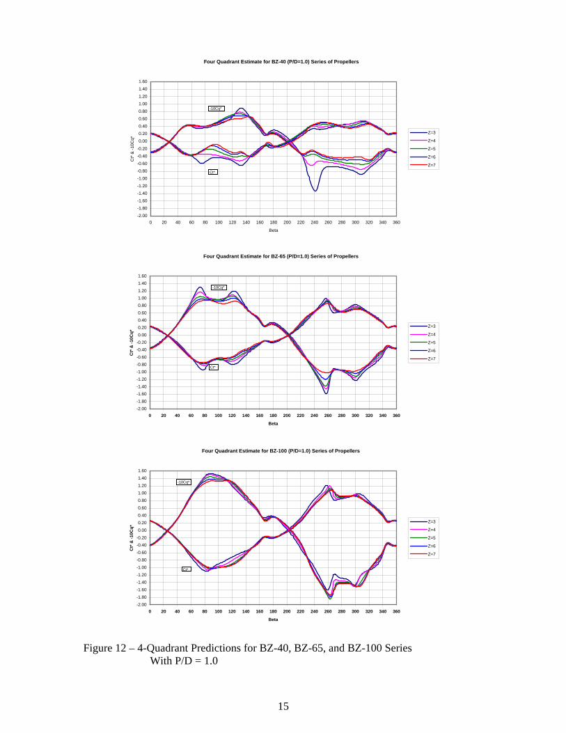
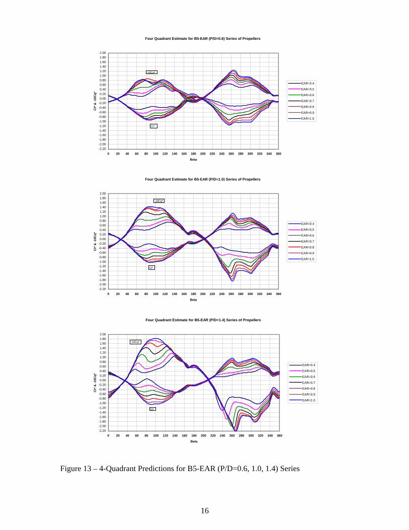
extrapolation. In the more well behaved Regions ‘A’ and ‘C’ ICE was specified to produce the single “best” solution, while in Regions ‘B’ and ‘D’ ICE was specified to produce 20 solutions and average these multiple solutions for a “final” solution. For all the ICE training the error measures were typically: AAM > 0.99 and r > 0.99, which correspond to excellent predictions. The penalty incurred with using four FFNN’s is that there are, inevitably, discontinuities at the boundaries when moving from one FFNN prediction to another. Although these breaks are typically small, two “matching polynomial” procedures were developed to smoothly fit a polynomial from one prediction to the other, thereby ensuring continuity. One procedure matches the slopes and the other matches both slope and curvature. The detailed derivation of these procedures is discussed in Appendix D. For the four-quadrant predictions the first method was used as the default with an option to use the second derivative method. A computer program was written to use the four FFNN’s and the matching polynomial algorithm to produce 4-quadrant predictions of a B-Series propeller, or family of propellers. The utilization of this program will be discussed later. DISCUSSION OF RESULTS The results show excellent agreement with the existing data and provide a good means for estimating 4-quadrant performance for the entire B-Screw Series. There are reasonable trends when the results are plotted as a family of propeller performance curves with the different members of the family varying P/D, or EAR, or Z. Even the results near the edges of the box defining the input data (Table 1) look reasonable but there is increased uncertainty in these results. Examples of predicted trends using the FFNN are presented in Figures 9 through 13. Figures 9 and 10 show the predicted trends for EAR sweeps for a 3 and 6 bladed propeller series along with the existing measured data for the only propeller in each series. These plots are two excellent examples of how well the FFNNs can predict the performance of propellers that have not been tested. The plots in Figure 11 show P/D variations from 0.4 to 1.4 for three different 5-bladed propeller series with EARs = 0.40, 0.65, and 1.00. The plots in Figure 12 show blade number variations from 3 to 7 for three different propeller series with P/D = 1.0 and EARs = 0.40, 0.65, and 1.00. The plots in Figure 13 show EAR variations from 0.4 to 1.0 for three different 5-bladed propeller series with P/Ds = 0.6, 1.0, and 1.4. These three sets of plots show the consistency in the FFNN predictions, and showcase the ability of the networks to make reasonable predictions for propellers that have not been tested. During the training there were two distinctly different solutions needed in different regions of the data. In the two regions around the bollard conditions, Regions ‘A’ and ‘C’, the best training resulted from standard ICE training runs with a single “best” solution. However, in the two regions around the zero rpm conditions, Regions ‘B’ and ‘D’, the best training resulted from ICE training runs with 20 averaged solutions. The 20 independent solutions are obtained by varying which data points belong to the training and validation sets. After the 20 solutions are obtained, they are averaged to provide a single best solution.

13

Figure 9 - Four Quadrant Prediction for B3-EAR (P/D=1.0) Propeller Series Showing Comparison with Measured Data; Symbols = Measured Data, Solid Lines = Predictions Figure 10 - Four Quadrant Prediction for B6-EAR (P/D=1.0) Propeller Series Showing Comparison with Measured Data; Symbols = Measured Data, Solid Lines = Predictions

-1.80

-1.60

-1.40

-1.20

-1.00

-0.80

-0.60

-0.40

-0.20

0.00

0.20

0.40

0.60

0.80

1.00

1.20

1.40

1.60

0 20 40 60 80 100 120 140 160 180 200 220 240 260 280 300 320 340 360

Beta

Ct*

& -1

0Cq*

EAR=0.50EAR=0.65EAR=0.80EAR=0.95

-1.8

-1.6

-1.4

-1.2

-1

-0.8

-0.6

-0.4

-0.2

0

0.2

0.4

0.6

0.8

1

1.2

1.4

0 20 40 60 80 100 120 140 160 180 200 220 240 260 280 300 320 340 360

Beta

Ct*

& -1

0Cq*

EAR=0.50EAR=0.65EAR=0.80EAR=0.95

14

Figure 11 – 4-Quadrant Predictions for a B5-40, B5-65, and B5-100 Series

Four Quadrant Estimate for B5-65 Series of Propellers

-2.20-2.00-1.80-1.60-1.40-1.20-1.00-0.80-0.60-0.40-0.200.000.200.400.600.801.001.201.401.60

0 20 40 60 80 100 120 140 160 180 200 220 240 260 280 300 320 340 360

Beta

Ct*

& -1

0Cq*

P/D = 0.4

P/D = 0.6

P/D = 0.8

P/D = 1.0

P/D = 1.2

P/D = 1.4Ct

-10Cq*


-2.20-2.00-1.80-1.60-1.40-1.20-1.00-0.80-0.60-0.40-0.200.000.200.400.600.801.001.201.401.601.802.00

0 20 40 60 80 100 120 140 160 180 200 220 240 260 280 300 320 340 360

Beta

Ct*

& -1

0Cq*

P/D=0.40

P/D=0.60

P/D=0.80

P/D=1.00

P/D=1.20

P/D=1.40

Ct*

-10Cq*


-1.40

-1.20

-1.00

-0.80

-0.60

-0.40

-0.20

0.00

0.20

0.40

0.60

0.80

1.00

1.20

0 20 40 60 80 100 120 140 160 180 200 220 240 260 280 300 320 340 360

Beta

Ct*

& -1

0Cq*

P/D=0.40

P/D=0.60

P/D=0.80

P/D=1.00

P/D=1.20

P/D=1.40Ct*

-10Cq*

15

Figure 12 – 4-Quadrant Predictions for BZ-40, BZ-65, and BZ-100 Series With P/D = 1.0

Four Quadrant Estimate for BZ-40 (P/D=1.0) Series of Propellers

-2.00

-1.80

-1.60

-1.40

-1.20

-1.00

-0.80

-0.60

-0.40

-0.20

0.00

0.20

0.40

0.60

0.80

1.00

1.20

1.40

1.60

0 20 40 60 80 100 120 140 160 180 200 220 240 260 280 300 320 340 360

Beta

Ct*

& -1

0Cq*

Z=3

Z=4

Z=5

Z=6

Z=7Ct*

-10Cq*


-2.00-1.80

-1.60-1.40-1.20

-1.00-0.80-0.60

-0.40-0.200.00

0.200.400.60

0.801.001.20

1.401.60

0 20 40 60 80 100 120 140 160 180 200 220 240 260 280 300 320 340 360

Beta

Ct*

& -1

0Cq*

Z=3

Z=4

Z=5

Z=6

Z=7

Ct*

-10Cq*


-2.00

-1.80

-1.60

-1.40

-1.20

-1.00

-0.80

-0.60

-0.40-0.20

0.00

0.20

0.40

0.60

0.80

1.00

1.20

1.40

1.60

0 20 40 60 80 100 120 140 160 180 200 220 240 260 280 300 320 340 360

Beta

Ct*

& -1

0Cq*

Z=3

Z=4

Z=5

Z=6

Z=7

Ct*

-10Cq*

16

Figure 13 – 4-Quadrant Predictions for B5-EAR (P/D=0.6, 1.0, 1.4) Series

Four Quadrant Estimate for B5-EAR (P/D=0.6) Series of Propellers

-2.20-2.00-1.80-1.60-1.40-1.20-1.00-0.80-0.60-0.40-0.200.000.200.400.600.801.001.201.401.601.802.00

0 20 40 60 80 100 120 140 160 180 200 220 240 260 280 300 320 340 360

Beta

Ct*

& -1

0Cq*

EAR=0.4

EAR=0.5

EAR=0.6

EAR=0.7

EAR=0.8

EAR=0.9

EAR=1.0

Ct*

-10Cq*


-2.20-2.00-1.80-1.60-1.40-1.20-1.00-0.80-0.60-0.40-0.200.000.200.400.600.801.001.201.401.601.802.00

0 20 40 60 80 100 120 140 160 180 200 220 240 260 280 300 320 340 360

Beta

Ct*

& -1

0Cq*

EAR=0.4

EAR=0.5

EAR=0.6

EAR=0.7

EAR=0.8

EAR=0.9

EAR=1.0

Ct*

-10Cq*


-2.20-2.00-1.80-1.60-1.40-1.20-1.00-0.80-0.60-0.40-0.200.000.200.400.600.801.001.201.401.601.802.00

0 20 40 60 80 100 120 140 160 180 200 220 240 260 280 300 320 340 360

Beta

Ct*

& -1

0Cq*

EAR=0.4

EAR=0.5

EAR=0.6

EAR=0.7

EAR=0.8

EAR=0.9

EAR=1.0

Ct*

-10Cq*

17

DUCTED PROPELLER SERIES FEED FORWARD NEURAL NETWORK DEVELOPMENT

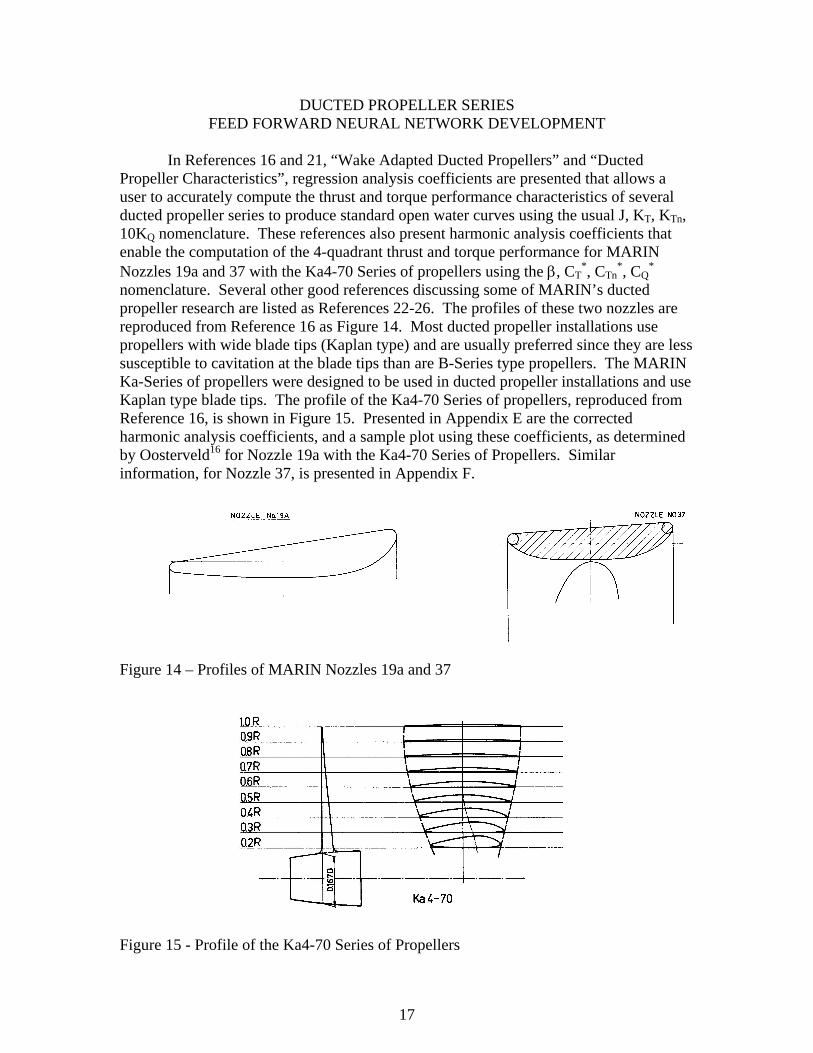
In References 16 and 21, “Wake Adapted Ducted Propellers” and “Ducted

Propeller Characteristics”, regression analysis coefficients are presented that allows a user to accurately compute the thrust and torque performance characteristics of several ducted propeller series to produce standard open water curves using the usual J, KT, KTn, 10KQ nomenclature. These references also present harmonic analysis coefficients that enable the computation of the 4-quadrant thrust and torque performance for MARIN Nozzles 19a and 37 with the Ka4-70 Series of propellers using the β, CT

*, CTn*, CQ

* nomenclature. Several other good references discussing some of MARIN’s ducted propeller research are listed as References 22-26. The profiles of these two nozzles are reproduced from Reference 16 as Figure 14. Most ducted propeller installations use propellers with wide blade tips (Kaplan type) and are usually preferred since they are less susceptible to cavitation at the blade tips than are B-Series type propellers. The MARIN Ka-Series of propellers were designed to be used in ducted propeller installations and use Kaplan type blade tips. The profile of the Ka4-70 Series of propellers, reproduced from Reference 16, is shown in Figure 15. Presented in Appendix E are the corrected harmonic analysis coefficients, and a sample plot using these coefficients, as determined by Oosterveld16 for Nozzle 19a with the Ka4-70 Series of Propellers. Similar information, for Nozzle 37, is presented in Appendix F.

Figure 14 – Profiles of MARIN Nozzles 19a and 37 Figure 15 - Profile of the Ka4-70 Series of Propellers

18

METHODOLOGY

The preparation of the input data was much more straightforward for these two ducted propellers series than for the B-Screw Series since the predictions of the FFNN training would be entirely interpolative. For these two ducts, values of CT

*, CTn* and CQ

* were computed from the coefficients shown in Appendices E and F at one degree β increments from 0 to 360 degrees. The FFNN training efforts with the B-Series showed that satisfactory interpolation of the data could be achieved when using only one network to predict the entire β range. Therefore, this was also tried with the ducted propeller data. Again, in addition to β and P/D, it was discovered that SIN and COS terms were needed as input to the training data. The typical terms that were important for both Nozzles 19a and 37 were: β, P/D, COS(β), COS(5β), SIN(β), SIN(5β), and SIN(10β). For all the ICE training the error measures were typically: AAM > 0.99 and r > 0.99, which correspond to excellent predictions.

Computer programs were written to use the FFNN’s to produce 4-quadrant

predictions for a Ka4-70 propeller in each nozzle. The utilization of this program will be discussed later.

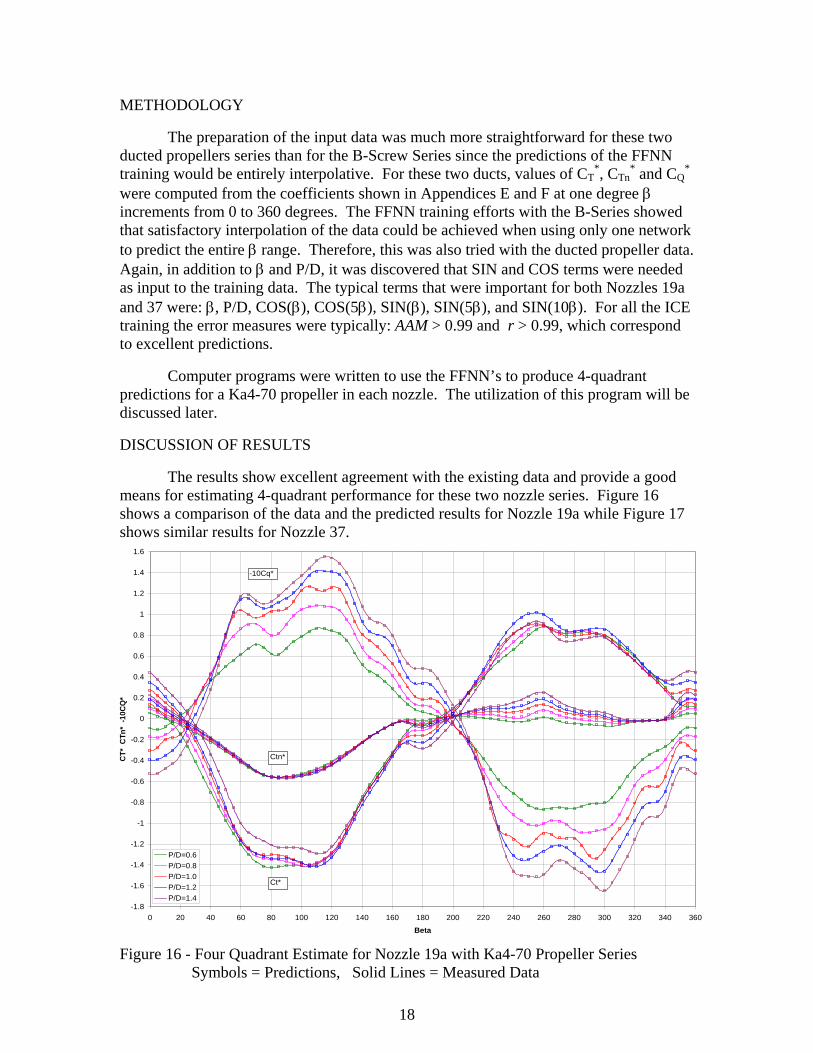
DISCUSSION OF RESULTS The results show excellent agreement with the existing data and provide a good means for estimating 4-quadrant performance for these two nozzle series. Figure 16 shows a comparison of the data and the predicted results for Nozzle 19a while Figure 17 shows similar results for Nozzle 37. Figure 16 - Four Quadrant Estimate for Nozzle 19a with Ka4-70 Propeller Series Symbols = Predictions, Solid Lines = Measured Data

-1.8

-1.6

-1.4

-1.2

-1

-0.8

-0.6

-0.4

-0.2

0

0.2

0.4

0.6

0.8

1

1.2

1.4

1.6

0 20 40 60 80 100 120 140 160 180 200 220 240 260 280 300 320 340 360

Beta

CT*

CTn

* -1

0CQ

*

P/D=0.6P/D=0.8P/D=1.0P/D=1.2P/D=1.4

Ct*

Ctn*

-10Cq*

19

Figure 17 - Four Quadrant Estimate for Nozzle 37 with Ka4-70 Propeller Series Symbols = Predictions, Solid Lines = Measured Data

UTILIZATION OF THE FFNNs FOR THE B-SCREW SERIES AND TWO DUCTED PROPELLER SERIES

Included with this report is a Compact Disc (CD) that contains five folders. The folder named “Bseries4Q” contains the executable program and data files, written as part of this project, to predict the thrust and torque performance of propellers within the range of the B-Screw Series. The folders named “N19Ka4704Q” and “N37Ka4704Q” contain the executable programs and data files for Nozzle 19a and Nozzle 37 respectively. The folder named “4Q Samples” contain several Microsoft Excel files that can be used as templates for plotting the output. The folder named “Extra” contains some programs that use the coefficients from Reference 14, and coefficients of a subset of the Hamilton Standard Air Screws (Reference 27), to perform propeller optimizations and off-design computations for several propeller types. Included in this folder are files describing the input and output variables.

All of the four-quadrant programs have the same basic user interface. Because of these similarities the following discussion will be limited to the B-Series prediction program contained in the folder “Bseries4Q”.

-1.8

-1.6

-1.4

-1.2

-1

-0.8

-0.6

-0.4

-0.2

0

0.2

0.4

0.6

0.8

1

1.2

1.4

1.6

0 20 40 60 80 100 120 140 160 180 200 220 240 260 280 300 320 340 360

Beta

CT*

CTn

* & -1

0CQ

*

P/D=0.6P/D=0.8P/D=1.0P/D=1.2P/D=1.4

Ct*

Ctn*

-10Cq*

20

The 4-quadrant prediction program runs in a command prompt window and has

two basic operational modes: 1 – predict the 4-quadrant performance of a single propeller; and, 2 – predict the 4-quadrant performance of a family of propellers. To install this program simply copy the executable program and the data files to a folder of choice. The program is run by double clicking on the program icon. To aid the user of this program, the command prompt windows from two sample runs are included as Tables 7 and 8. The sample run shown in Table 7 represents the case where the user wishes to make a prediction for a single B-series propeller with four blades, a P/D=0.8, and an EAR=0.7. The yellow highlighted text is user input. The rest of the text is program output. The main output from the program is put in a ‘comma separated variable’(csv) file named by the user. This file can be easily used to plot the data in the plotting program of the user’s liking. If Excel is used to plot the data the template files included with the CD can ease the task of plotting. The next to the last user input starts out with the question, “What Heading do you wish printed with the output.” This input has little meaning for a single propeller prediction but is important for multiple propeller predictions and will be discussed later. Table 7 - Sample of a Single Propeller Prediction Run: Program to Produce 4-Quadrant Open-water Characteristics Based on the Wageningen B-Series Test Results DO YOU WISH TO: 0 - Exit Program 1 - Produce estimates for a Single Propeller 2 - Produce estimates for a Family of Propellers ENTER CHOICE - - 1 Enter the Propeller P/D - - 0.8 Enter the Number of Blades - - 4 Enter the Propeller EAR - - 0.7 What Heading do you wish printed with the output: 0 - No Heading 1 - Propeller P/D 2 - Propeller Blade Number Z 3 - Propeller Expanded Area Ratio EAR ENTER CHOICE - - 1 Enter the name of the output file without extension - - sample1 Program Terminated Normally

21

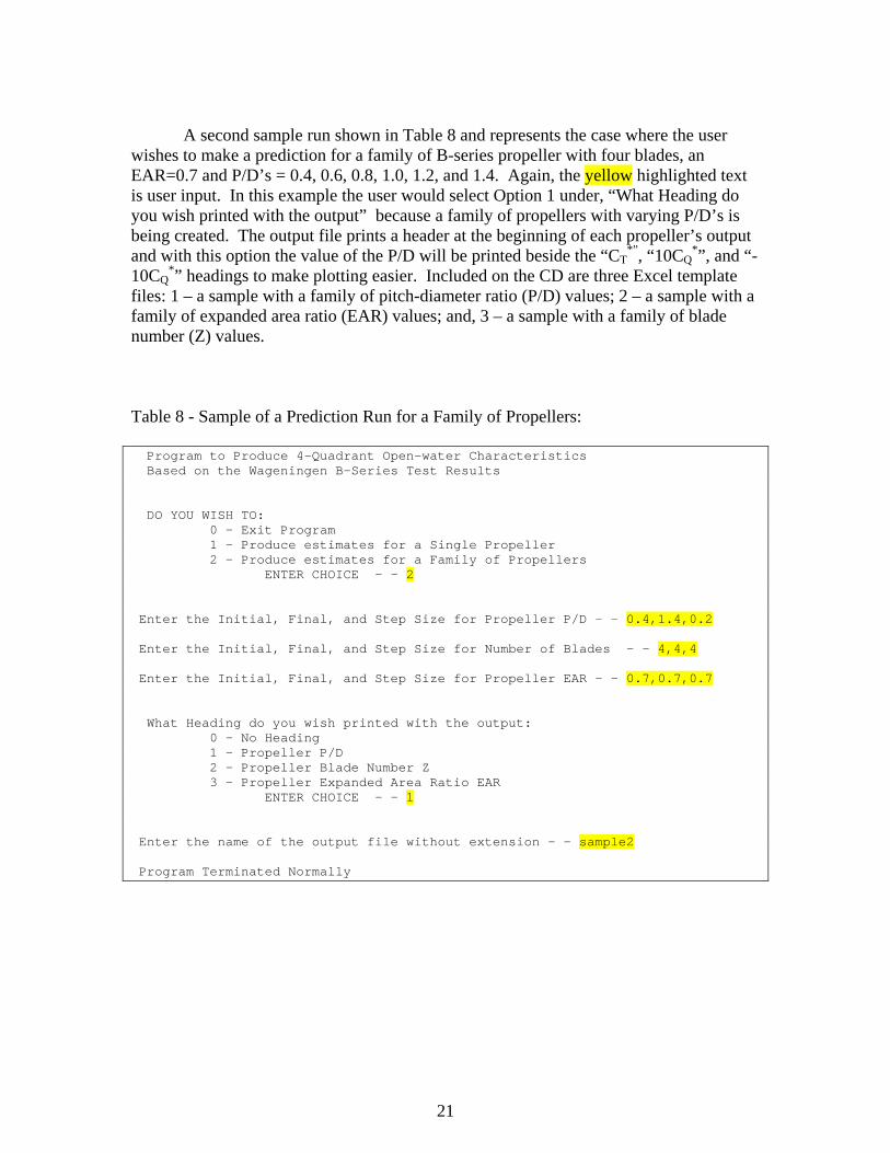
A second sample run shown in Table 8 and represents the case where the user wishes to make a prediction for a family of B-series propeller with four blades, an EAR=0.7 and P/D’s = 0.4, 0.6, 0.8, 1.0, 1.2, and 1.4. Again, the yellow highlighted text is user input. In this example the user would select Option 1 under, “What Heading do you wish printed with the output” because a family of propellers with varying P/D’s is being created. The output file prints a header at the beginning of each propeller’s output and with this option the value of the P/D will be printed beside the “CT

*”, “10CQ*”, and “-

10CQ*” headings to make plotting easier. Included on the CD are three Excel template

files: 1 – a sample with a family of pitch-diameter ratio (P/D) values; 2 – a sample with a family of expanded area ratio (EAR) values; and, 3 – a sample with a family of blade number (Z) values. Table 8 - Sample of a Prediction Run for a Family of Propellers: Program to Produce 4-Quadrant Open-water Characteristics Based on the Wageningen B-Series Test Results DO YOU WISH TO: 0 - Exit Program 1 - Produce estimates for a Single Propeller 2 - Produce estimates for a Family of Propellers ENTER CHOICE - - 2 Enter the Initial, Final, and Step Size for Propeller P/D - - 0.4,1.4,0.2 Enter the Initial, Final, and Step Size for Number of Blades - - 4,4,4 Enter the Initial, Final, and Step Size for Propeller EAR - - 0.7,0.7,0.7 What Heading do you wish printed with the output: 0 - No Heading 1 - Propeller P/D 2 - Propeller Blade Number Z 3 - Propeller Expanded Area Ratio EAR ENTER CHOICE - - 1 Enter the name of the output file without extension - - sample2 Program Terminated Normally

22

CONCLUSIONS AND RECOMMENDATIONS

For all the neural network training the error measures were typically: AAM > 0.99

and R > 0.99, which correspond to excellent predictions. The results show excellent agreement with the existing data and provide a good means for estimating 4-quadrant performance for the entire B-Screw Series and for the two nozzle series also investigated. Examination of the results show how well the FFNNs can predict the performance for propellers that have not been tested. For the B-Screw Series there are reasonable trends when the results are plotted as families of propeller performance curves with the different members of the family varying P/D, or EAR, or Z. The programs, and files, included herein allow for the easy determination of any propeller within the data sets.

Extending the results of the two nozzle series is recommended. Past work by the author has shown that reasonable estimates of ducted propeller performance can be made using modifications to the B-Screw Series and using velocity and nozzle loading computations from Reference 16.

23

REFERENCES [Note: The bold notations below indicate which screws of the B-Series are discussed in the referenced report.] 1. Lammeren, W.P.A. van, “Resultaten van Voortgezette Systematische Proeven met

Vrijvarende 4-bladige Schroeven, type B4.40 en B4.55”, Het Schip 19, No. 8, pp.104, 1937. NSMB Publication No. 28. [B4-40, B4-55]

2. Lammeren, W.P.A. van, “Scheepsmodel en Scheepsproeven”, Schip en Werf,1937, pp.84 and 104. NSMB Publication No. 29. [B4-40, B4-55]

3. Troost, L., “Open Water Test Series with Modern Propeller Forms”, Transactions North East Coast Institution of Engineers and Shipbuilders, 1938, pp. 321. NSMB Publication No. 33. [A4-40,B4-40, B4-55]

4. Troost, L., “Open Water Test Series with Modern Propeller Forms, Part 2”, Transactions North East Coast Institution of Engineers and Shipbuilders, 1940, pp. 91. NSMB Publication No. 42. [B3-35, B3-50]

5. Lammeren, W.P.A. van, “Enige gezichtspunten bij het ontwerpen van Scheepsschroeven”, Schip en Werf, 1940, pp, 88, 151 and 163. NSMB Publication No. 45. [B3-35, B3-50]

6. Lammeren, W.P.A. van, “Weerstand en Voortstuwing van Schepen”, De Technische Boekhandel H. Stam, Amsterdam, 1942. NSMB Publication No. 51. [A4-40,B3-35,B3-50,B4-40, B4-55]

7. Lammeren, W.P.A. van, “Weerstand en Voortstuwing van Schepen, Beknopte Uitgave.”, De Technische Boekhandel H. Stam, Amsterdam, 1946. NSMB Publication No. 55. [A4-40,B3-35,B3-50,B4-40, B4-55]

8. Lammeren, W.P.A. van, Troost, L., Koning, J.G., “Resistance, Propulsion and Steering of Ships”, De Technische Boekhandel H. Stam, Amsterdam, 1948. NSMB Publication No. 75. [B3-35,B3-50,B4-40, B4-55]

9. Lammeren, W.P.A. van, Aken, J.A. van, “Een Uitbreiding van de Systematische 3- en 4-bladige Schroefseries van het Nederlands Scheepsbouwkundig Proefstation, Schip en Werf, 1949, No. 13, NSMB Publication No. 78. [B3-35,B3-50,B3-65, B4-40, B4-55,B4-70]

10. Troost, L., “Open Water Test Series with Modern Propeller Forms, Part 3: Two and Five Bladed Propellers”, Transactions North East Coast Institution of Engineers and Shipbuilders, Vol. 67, 1951. [B2-30,B3-35,B3-50,B3-65, B4-40, B4-55,B4-70,B5-45,B5-60]

11. Lammeren, W.P.A. van, “Resultaten vanele Voortgezette Systematische Proefnemingen met 2- en 5-bladige Schroefseries”, Schip en Werf, 1951, No. 8, [B2-30,B5-45,B5-60]

12. Lammeren, W.P.A. van, Manen, J.D. van, Oosterveld, M.W.C., “The Wageningen B-Screw Series”, Transactions SNAME, Vol. 77, pp. 269-317, 1969. Schip en Werf, 1970, No. 5, pp. 88-103, No. 6, pp. 115-124. [B4-40,B4-55,B4-70,B4-85, B4-100,B5-45, B5-60,B5-75,B5-105, Four Quadrants, Effects of cavitation on B4-85,B4-100,B5-75,B5-105]

13. Oosterveld, M.W.C., Oossanen, P. van, “Representation of Propeller Characteristics Suitable for Preliminary Design Studies”, International Conference on Computer Applications in the Automation of Shipyard Operation and Ship Design, Tokyo, 1973, NSMB Publication No. 447

24

14. Oosterveld, M.W.C., Oossanen, P. van, “Recent Developments in Marine Propeller Hydrodynamics”, International Jubilee Meeting 40th Anniversary of the Netherlands Ship Model Basin, 1972, NSMB Publication No. 433

15. "Vier_Kwadrant Vrijvarende-Schroef-Karakterstieken Voor B-Serie Schroeven. Fourier-Reeks Ontwikkeling en Operationeel Gebruik", MARIN Report 60482-1-MS, 1984 [Limited Availability]

16. Oosterveld, M.W.C., “Wake Adapted Ducted Propellers”, (1970), NSMB Publication No. 345

17. Kuiper, G, “The Wageningen Propeller Series”, 1992, MARIN Publication No. 92-001

18. Faller, W.E., Smith, W.E., and Huang, T.T. “Applied Dynamic System Modeling: Six Degree-Of-Freedom Simulation Of Forced Unsteady Maneuvers Using Recursive Neural Networks”, 35th AIAA Aerospace Sciences Meeting, Paper 97-0336, 1997, pp. 1-46

19. Hess, D.E. and Faller, W.E. “Simulation of Ship Maneuvers Using Recursive Neural Networks,” 23rd Symposium on Naval Hydrodynamics, Val de Reuil, France, September 17-22, 2000

20. Ammeen, E. S., “Evaluation of Correlation Measures”, Naval Surface Warfare Center Report CRDKNSWC-HD-0406-01, March 1994

21. Oosterveld, M.W.C., “Ducted Propeller Characteristics”, Royal Institution of Naval Architects Symposium on Ducted Propellers, 1973

22. Manen, J.D. van, “Open-Water Test Series with Propellers in Nozzles”, International Shipbuilding Progress, Volume 1, Number 2, 1954

23. Manen, J.D. van, “Recent Research on Propellers in Nozzles”, Journal of Ship Research (SNAME), Volume 1, Number 2, July 1957

24. Manen, J.D. van, Oosterveld, M.W.C., “Analysis of Ducted-Propeller Design”, Society of Naval Architects and Marine Engineers Transactions, Volume 74, 1966

25. Oosterveld, M.W.C., “Ducted Propeller Systems Suitable for Tugs and Pushboats”, Great Lakes & Great Rivers Section SNAME, May, 1971

26. Oosterveld, M.W.C., Oortmerssen, G. van, “Thruster Systems for Improving the Maneuverability and Position-Keeping Capability of Floating Objects”, Offshore Technology Conference, 1972

27. “Generalized Method of Propeller Performance Estimation”, Hamilton Standard Report PDB 6101, Revision A, 1963

A-1

APPENDIX A

Summary of Coefficients and Results From

“Recent Developments in Marine Propeller Hydrodynamics” (Reference 14)

A-2

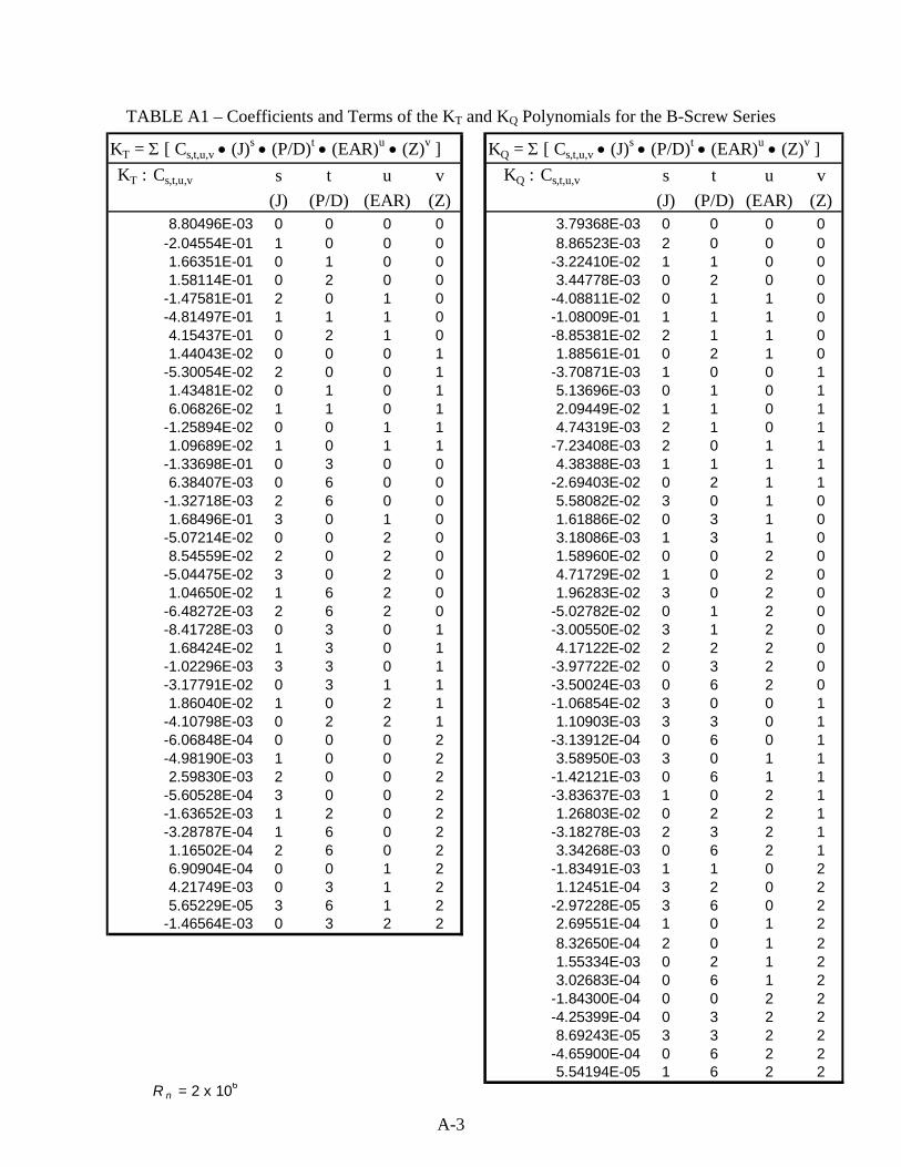
The open-water characteristics of the Wageningen B-Screw Series were faired, and cross-faired, by means of multiple regression analyses, and the results are presented in Reference 14. The regression analyses used the data from all of the 120 propeller models comprising the B-Series. All of the data was corrected to a Reynolds number of 2x106. The resulting polynomials were in the form of:

KT = f1(J, P/D, EAR, Z) and

KQ = f2(J, P/D, EAR, Z).

The polynomial results of the regression analyses are presented in Table A1, and a sample set of open water curves for the B4-70 series of propellers, produced from these polynomials, are presented in Figure A1.

A-3

TABLE A1 – Coefficients and Terms of the KT and KQ Polynomials for the B-Screw Series

KT = Σ [ Cs,t,u,v • (J)s • (P/D)t • (EAR)u • (Z)v ] KQ = Σ [ Cs,t,u,v • (J)s • (P/D)t • (EAR)u • (Z)v ]KT : Cs,t,u,v s t u v KQ : Cs,t,u,v s t u v

(J) (P/D) (EAR) (Z) (J) (P/D) (EAR) (Z)8.80496E-03 0 0 0 0 3.79368E-03 0 0 0 0

-2.04554E-01 1 0 0 0 8.86523E-03 2 0 0 01.66351E-01 0 1 0 0 -3.22410E-02 1 1 0 01.58114E-01 0 2 0 0 3.44778E-03 0 2 0 0

-1.47581E-01 2 0 1 0 -4.08811E-02 0 1 1 0-4.81497E-01 1 1 1 0 -1.08009E-01 1 1 1 04.15437E-01 0 2 1 0 -8.85381E-02 2 1 1 01.44043E-02 0 0 0 1 1.88561E-01 0 2 1 0

-5.30054E-02 2 0 0 1 -3.70871E-03 1 0 0 11.43481E-02 0 1 0 1 5.13696E-03 0 1 0 16.06826E-02 1 1 0 1 2.09449E-02 1 1 0 1

-1.25894E-02 0 0 1 1 4.74319E-03 2 1 0 11.09689E-02 1 0 1 1 -7.23408E-03 2 0 1 1

-1.33698E-01 0 3 0 0 4.38388E-03 1 1 1 16.38407E-03 0 6 0 0 -2.69403E-02 0 2 1 1

-1.32718E-03 2 6 0 0 5.58082E-02 3 0 1 01.68496E-01 3 0 1 0 1.61886E-02 0 3 1 0

-5.07214E-02 0 0 2 0 3.18086E-03 1 3 1 08.54559E-02 2 0 2 0 1.58960E-02 0 0 2 0

-5.04475E-02 3 0 2 0 4.71729E-02 1 0 2 01.04650E-02 1 6 2 0 1.96283E-02 3 0 2 0

-6.48272E-03 2 6 2 0 -5.02782E-02 0 1 2 0-8.41728E-03 0 3 0 1 -3.00550E-02 3 1 2 01.68424E-02 1 3 0 1 4.17122E-02 2 2 2 0

-1.02296E-03 3 3 0 1 -3.97722E-02 0 3 2 0-3.17791E-02 0 3 1 1 -3.50024E-03 0 6 2 01.86040E-02 1 0 2 1 -1.06854E-02 3 0 0 1

-4.10798E-03 0 2 2 1 1.10903E-03 3 3 0 1-6.06848E-04 0 0 0 2 -3.13912E-04 0 6 0 1-4.98190E-03 1 0 0 2 3.58950E-03 3 0 1 12.59830E-03 2 0 0 2 -1.42121E-03 0 6 1 1

-5.60528E-04 3 0 0 2 -3.83637E-03 1 0 2 1-1.63652E-03 1 2 0 2 1.26803E-02 0 2 2 1-3.28787E-04 1 6 0 2 -3.18278E-03 2 3 2 11.16502E-04 2 6 0 2 3.34268E-03 0 6 2 16.90904E-04 0 0 1 2 -1.83491E-03 1 1 0 24.21749E-03 0 3 1 2 1.12451E-04 3 2 0 25.65229E-05 3 6 1 2 -2.97228E-05 3 6 0 2

-1.46564E-03 0 3 2 2 2.69551E-04 1 0 1 28.32650E-04 2 0 1 21.55334E-03 0 2 1 23.02683E-04 0 6 1 2

-1.84300E-04 0 0 2 2-4.25399E-04 0 3 2 28.69243E-05 3 3 2 2

-4.65900E-04 0 6 2 25.54194E-05 1 6 2 2

R n = 2 x 106

A-4

Figure A1 – B4-70 Series of Open-Water Curves from Regression Analysis Coefficients

Open-Water Curves for B4-70 Propellers

0

0.1

0.2

0.3

0.4

0.5

0.6

0.7

0.8

0.9

1

1.1

1.2

1.3

0 0.1 0.2 0.3 0.4 0.5 0.6 0.7 0.8 0.9 1 1.1 1.2 1.3 1.4 1.5 1.6

J

KT

10K

Q

Eta

P/D=0.4P/D=0.6P/D=0.8P/D=1.0P/D=1.2P/D=1.4

B-1

APPENDIX B

Summary of Coefficients and Results From

“Vier_Kwadrant Vrijvarende-Schroef-Karakterstieken Voor B-Serie Schroeven. Fourier-Reeks Ontwikkeling en Operationeel Gebruik”

(Reference 15)

B-2

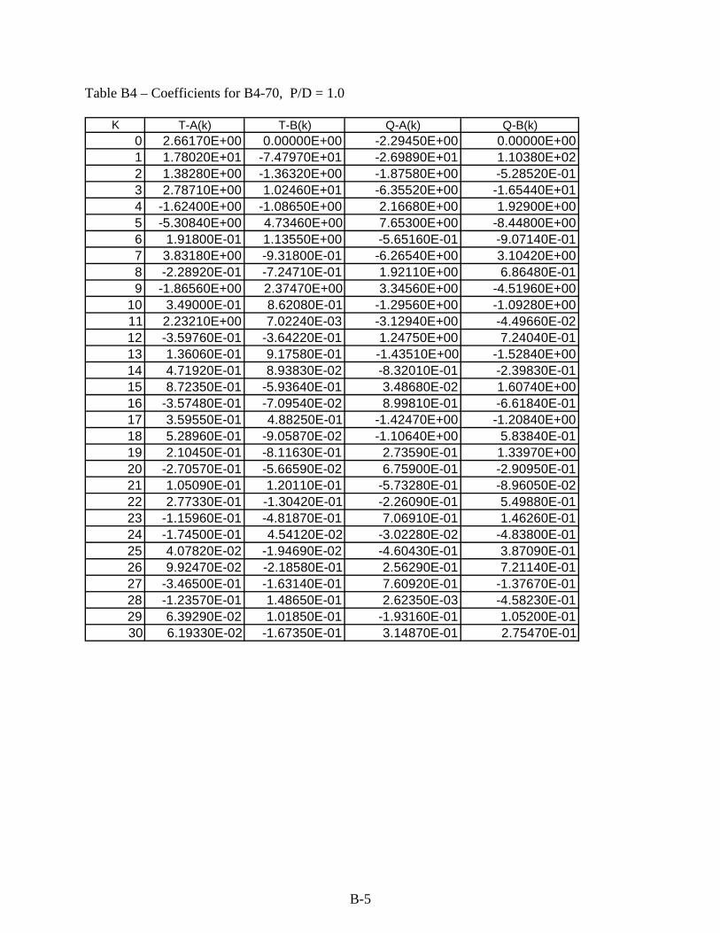
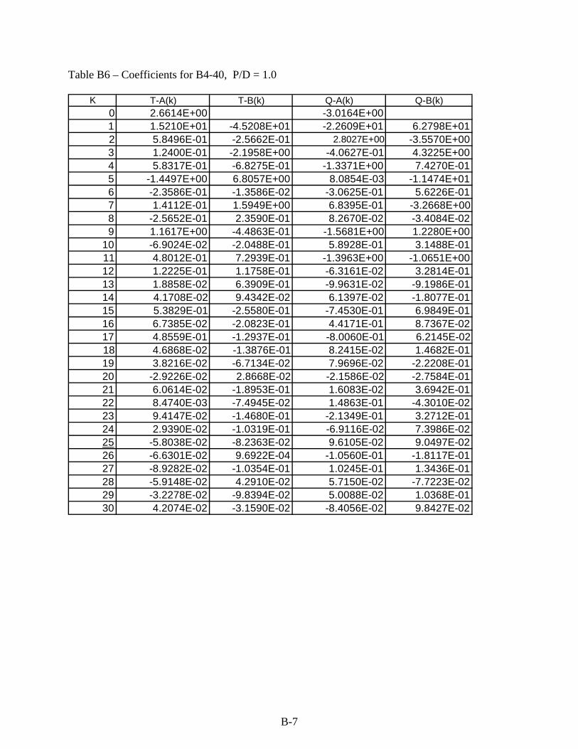
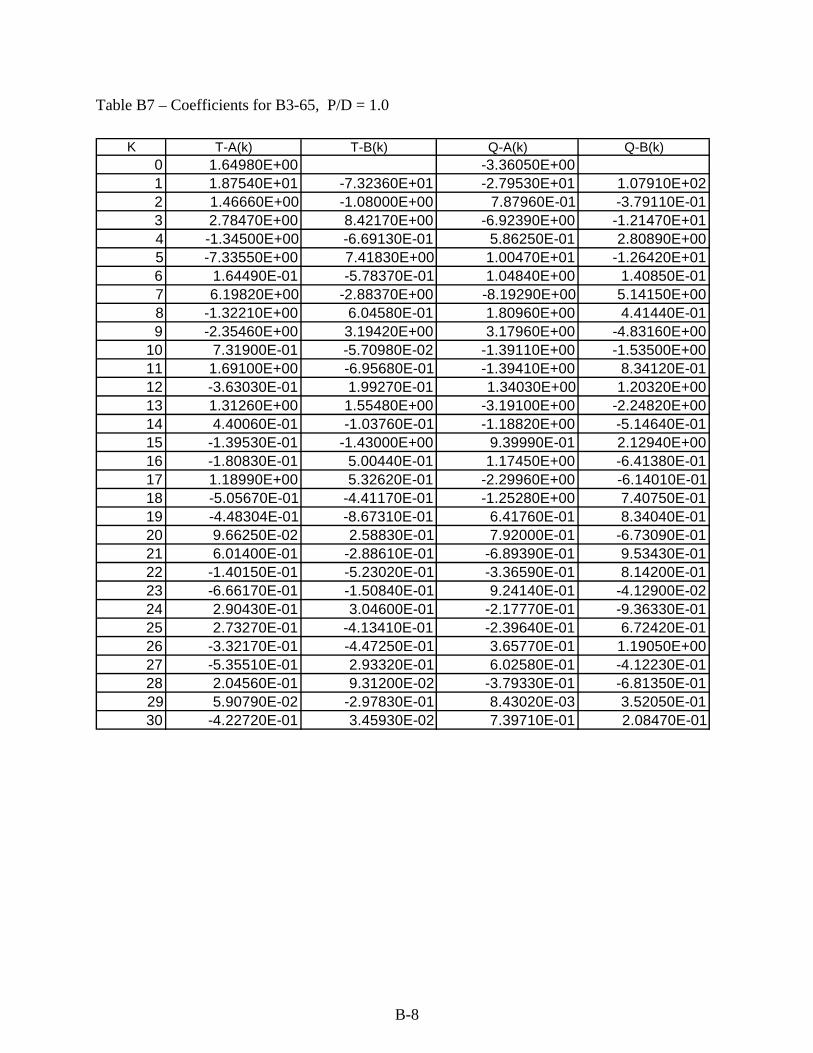
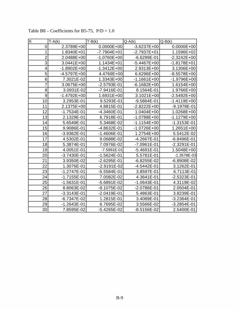
The open-water characteristics of a subset of the Wageningen B-Screw Series were faired by means of harmonic analyses, and the results are presented in Reference 15. The analyses used the data from 14 of the 120 propeller models comprising the B-Series. The characteristics of the 14 propellers are presented in Table B1. The resulting harmonic analysis coefficients are presented in Tables B2 through B15 and are in the form of:

( ) ( ){ }∑=

+=30

0

* sin)(cos)(100

1k

T kkBkkAC ββ

( ) ( ){ }∑=

+−

=30

0

* sin)(cos)(1000

1k

Q kkBkkAC ββ .

Four quadrant plots, for all 14 propellers, generated from these coefficients are presented in Figures B1 through B3. Table B1 – Propellers for Which MARIN has 4-Quadrant Results

No. B-Series P/D EAR Z1 4-100 1.0 1.00 42 4-85 1.0 0.85 43 4-70 1.0 0.70 44 4-55 1.0 0.55 45 4-40 1.0 0.40 46 3-65 1.0 0.65 37 5-75 1.0 0.75 58 6-80 1.0 0.80 69 7-85 1.0 0.85 710 4-70 0.5 0.70 411 4-70 0.6 0.70 412 4-70 0.8 0.70 413 4-70 1.2 0.70 414 4-70 1.4 0.70 4

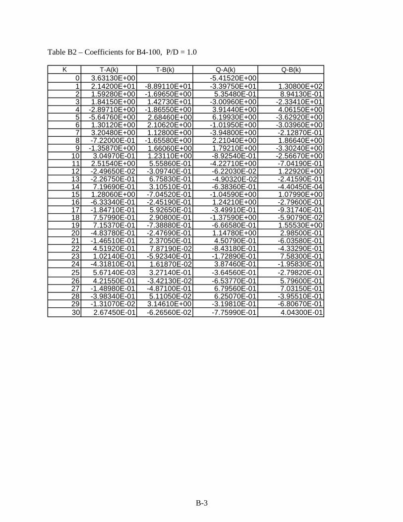
B-3

Table B2 – Coefficients for B4-100, P/D = 1.0

K T-A(k) T-B(k) Q-A(k) Q-B(k)0 3.63130E+00 -5.41520E+001 2.14200E+01 -8.89110E+01 -3.39750E+01 1.30800E+022 1.59280E+00 -1.69650E+00 5.35480E-01 8.94130E-013 1.84150E+00 1.42730E+01 -3.00960E+00 -2.33410E+014 -2.89710E+00 -1.86550E+00 3.91440E+00 4.06150E+005 -5.64760E+00 2.68460E+00 6.19930E+00 -3.62920E+006 1.30120E+00 2.10620E+00 -1.01950E+00 -3.03960E+007 3.20480E+00 1.12800E+00 -3.94800E+00 -2.12870E-018 -7.22000E-01 -1.65580E+00 2.21040E+00 1.86640E+009 -1.35870E+00 1.66060E+00 1.79210E+00 -3.30240E+00

10 3.04970E-01 1.23110E+00 -8.92540E-01 -2.56670E+0011 2.51540E+00 5.55860E-01 -4.22710E+00 -7.04190E-0112 -2.49650E-02 -3.09740E-01 -6.22030E-02 1.22920E+0013 -2.26750E-01 6.75830E-01 -4.90320E-02 -2.41590E-0114 7.19690E-01 3.10510E-01 -6.38360E-01 -4.40450E-0415 1.28060E+00 -7.04520E-01 -1.04590E+00 1.07990E+0016 -6.33340E-01 -2.45190E-01 1.24210E+00 -2.79600E-0117 -1.84710E-01 5.92650E-01 -3.49910E-01 -9.31740E-0118 7.57990E-01 2.90800E-01 -1.37590E+00 -5.90790E-0219 7.15370E-01 -7.38880E-01 -6.66580E-01 1.55530E+0020 -4.83780E-01 -2.47690E-01 1.14780E+00 2.98500E-0121 -1.46510E-01 2.37050E-01 4.50790E-01 -6.03580E-0122 4.51920E-01 7.87190E-02 -8.43180E-01 -4.33290E-0123 1.02140E-01 -5.92340E-01 -1.72890E-01 7.58300E-0124 -4.31810E-01 1.61870E-02 3.87460E-01 -1.95830E-0125 5.67140E-03 3.27140E-01 -3.64560E-01 -2.79820E-0126 4.21550E-01 -3.42130E-02 -6.53770E-01 5.79600E-0127 -1.48980E-01 -4.87100E-01 6.79560E-01 7.03150E-0128 -3.98340E-01 5.11050E-02 6.25070E-01 -3.95510E-0129 -1.31070E-02 3.14610E+00 -3.19810E-01 -6.80670E-0130 2.67450E-01 -6.26560E-02 -7.75990E-01 4.04300E-01

B-4


K T-A(k) T-B(k) Q-A(k) Q-B(k)0 2.61020E+00 -3.77070E+001 1.97800E+01 -8.33850E+01 -3.12200E+01 1.23610E+022 2.54730E+00 -1.38420E+00 -1.19200E+00 2.65230E-013 1.93370E+00 1.32140E+01 -3.72570E+00 -2.14800E+014 -3.02980E+00 -1.46910E+00 4.27760E+00 3.62570E+005 -5.07970E+00 3.38520E+00 6.29120E+00 -5.10650E+006 9.60500E-01 1.59360E+00 -1.36150E+00 -2.54140E+007 3.20350E+00 -2.50440E-02 -4.63510E+00 1.16680E+008 -4.85220E-01 -1.11150E+00 2.04310E+00 1.54370E+009 -1.59270E+00 1.98010E+00 2.70370E+00 -3.61520E+0010 6.66310E-02 9.76360E-01 -1.04690E+00 -1.76560E+0011 2.28780E+00 4.10250E-01 -4.17300E+00 -5.18810E-0112 1.11679E-03 -2.78470E-01 3.61370E-01 8.77590E-0113 7.39610E-02 7.48720E-01 -2.83690E-01 -5.20160E-0114 5.95000E-01 9.56370E-02 -7.84570E-01 1.75330E-0115 1.06090E+00 -5.59690E-01 -9.50780E-01 1.12170E+0016 -6.39530E-01 -6.81720E-02 1.38380E+00 -5.60010E-0117 8.21220E-02 4.98030E-01 -5.14360E-01 -8.45910E-0118 7.82040E-01 1.44770E-01 -1.41850E+00 3.00220E-0119 5.70900E-01 -7.81110E-01 -3.42780E-01 1.56160E+0020 -3.69140E-01 -1.99970E-01 1.09120E+00 -1.84230E-0221 -3.28850E-02 1.81400E-01 5.28720E-02 -4.23940E-0122 3.38950E-01 -3.43120E-02 -6.49710E-01 1.28520E-0123 -1.16470E-01 -5.51440E-01 2.42770E-01 5.53450E-0124 -2.58010E-01 6.32890E-02 2.56870E-01 -3.91650E-0125 6.20520E-02 1.97350E-01 -4.18820E-01 -3.07760E-0226 2.81050E-01 -2.02560E-01 -3.36110E-01 7.50880E-0127 -3.31890E-01 -3.71340E-01 7.88260E-01 -3.02830E-0128 -9.12000E-01 1.69250E-01 3.96350E-01 -6.90500E-0129 6.21630E-02 2.79360E-01 -4.93400E-01 -2.56730E-0130 1.55370E-01 -1.52450E-01 -2.62130E-01 6.26530E-01

B-5


K T-A(k) T-B(k) Q-A(k) Q-B(k)0 2.66170E+00 0.00000E+00 -2.29450E+00 0.00000E+001 1.78020E+01 -7.47970E+01 -2.69890E+01 1.10380E+022 1.38280E+00 -1.36320E+00 -1.87580E+00 -5.28520E-013 2.78710E+00 1.02460E+01 -6.35520E+00 -1.65440E+014 -1.62400E+00 -1.08650E+00 2.16680E+00 1.92900E+005 -5.30840E+00 4.73460E+00 7.65300E+00 -8.44800E+006 1.91800E-01 1.13550E+00 -5.65160E-01 -9.07140E-017 3.83180E+00 -9.31800E-01 -6.26540E+00 3.10420E+008 -2.28920E-01 -7.24710E-01 1.92110E+00 6.86480E-019 -1.86560E+00 2.37470E+00 3.34560E+00 -4.51960E+00

10 3.49000E-01 8.62080E-01 -1.29560E+00 -1.09280E+0011 2.23210E+00 7.02240E-03 -3.12940E+00 -4.49660E-0212 -3.59760E-01 -3.64220E-01 1.24750E+00 7.24040E-0113 1.36060E-01 9.17580E-01 -1.43510E+00 -1.52840E+0014 4.71920E-01 8.93830E-02 -8.32010E-01 -2.39830E-0115 8.72350E-01 -5.93640E-01 3.48680E-02 1.60740E+0016 -3.57480E-01 -7.09540E-02 8.99810E-01 -6.61840E-0117 3.59550E-01 4.88250E-01 -1.42470E+00 -1.20840E+0018 5.28960E-01 -9.05870E-02 -1.10640E+00 5.83840E-0119 2.10450E-01 -8.11630E-01 2.73590E-01 1.33970E+0020 -2.70570E-01 -5.66590E-02 6.75900E-01 -2.90950E-0121 1.05090E-01 1.20110E-01 -5.73280E-01 -8.96050E-0222 2.77330E-01 -1.30420E-01 -2.26090E-01 5.49880E-0123 -1.15960E-01 -4.81870E-01 7.06910E-01 1.46260E-0124 -1.74500E-01 4.54120E-02 -3.02280E-02 -4.83800E-0125 4.07820E-02 -1.94690E-02 -4.60430E-01 3.87090E-0126 9.92470E-02 -2.18580E-01 2.56290E-01 7.21140E-0127 -3.46500E-01 -1.63140E-01 7.60920E-01 -1.37670E-0128 -1.23570E-01 1.48650E-01 2.62350E-03 -4.58230E-0129 6.39290E-02 1.01850E-01 -1.93160E-01 1.05200E-0130 6.19330E-02 -1.67350E-01 3.14870E-01 2.75470E-01

B-6


K T-A(k) T-B(k) Q-A(k) Q-B(k)0 3.40640E+00 -4.41640E+001 1.61450E+01 -6.34110E+01 -2.44340E+01 8.87710E+012 1.75060E-01 -1.13890E+00 3.34920E+00 -2.68910E+003 2.92210E+00 5.20750E+00 -4.97930E+00 -5.51560E+004 -5.68750E-01 -8.29960E-01 -1.36050E+00 3.09920E+005 -5.29070E+00 6.42560E+00 4.67430E+00 -1.27140E+016 1.56410E-01 9.28550E-01 1.37913E-01 -1.51580E+007 3.92110E+00 -5.91790E-01 -1.94810E+00 2.82940E+008 -5.06890E-01 -3.79970E-01 2.68480E+00 1.15950E+009 -1.44370E+00 1.85180E-01 -1.03960E+00 -2.86520E+00

10 5.50050E-01 3.81780E-01 -2.25050E+00 -4.66420E-0111 1.19860E+00 -6.60590E-02 2.91140E-01 -1.16780E+0012 -2.35430E-01 -2.74010E-02 1.13700E+00 -9.19040E-0113 6.52410E-01 1.00850E+00 -2.51870E+00 8.69490E-0214 2.86880E-01 -1.37120E-01 2.38060E-01 1.46420E+0015 1.73000E-01 -6.97130E-01 -4.22290E-03 1.27800E-0116 -2.11270E-01 2.70740E-01 -6.74320E-01 -1.33320E+0017 6.79660E-01 4.36890E-01 -7.66300E-01 3.96200E-0118 2.63910E-01 -3.26280E-01 6.02540E-01 7.53620E-0119 -1.09450E-01 -5.47540E-01 -1.92280E-01 -1.92350E-0120 2.22400E-02 1.42420E-01 -6.30170E-01 3.94520E-0121 3.36990E-01 -1.40120E-01 -3.97380E-02 1.06240E+0022 -1.38770E-01 -2.36280E-01 6.61970E-01 -6.51970E-0123 -3.11400E-01 -1.11840E-01 -1.94840E-01 -1.80340E-0124 1.08280E-01 1.79980E-01 -2.90960E-01 6.15580E-0125 1.17050E-01 -1.87770E-01 6.93270E-01 4.43970E-0126 -4.85670E-02 -1.09040E-01 1.59870E-02 -2.79230E-0127 -1.92100E-01 1.30360E-02 -3.42590E-01 9.71600E-0228 1.37410E-01 -3.66280E-02 3.65600E-01 1.92180E-0129 -6.01250E-02 -9.93000E-02 5.03790E-01 -4.17570E-0130 -1.32570E-01 -1.57540E-02 -4.38070E-01 -3.00540E-01

B-7


K T-A(k) T-B(k) Q-A(k) Q-B(k)0 2.6614E+00 -3.0164E+001 1.5210E+01 -4.5208E+01 -2.2609E+01 6.2798E+012 5.8496E-01 -2.5662E-01 2.8027E+00 -3.5570E+003 1.2400E-01 -2.1958E+00 -4.0627E-01 4.3225E+004 5.8317E-01 -6.8275E-01 -1.3371E+00 7.4270E-015 -1.4497E+00 6.8057E+00 8.0854E-03 -1.1474E+016 -2.3586E-01 -1.3586E-02 -3.0625E-01 5.6226E-017 1.4112E-01 1.5949E+00 6.8395E-01 -3.2668E+008 -2.5652E-01 2.3590E-01 8.2670E-02 -3.4084E-029 1.1617E+00 -4.4863E-01 -1.5681E+00 1.2280E+00

10 -6.9024E-02 -2.0488E-01 5.8928E-01 3.1488E-0111 4.8012E-01 7.2939E-01 -1.3963E+00 -1.0651E+0012 1.2225E-01 1.1758E-01 -6.3161E-02 3.2814E-0113 1.8858E-02 6.3909E-01 -9.9631E-02 -9.1986E-0114 4.1708E-02 9.4342E-02 6.1397E-02 -1.8077E-0115 5.3829E-01 -2.5580E-01 -7.4530E-01 6.9849E-0116 6.7385E-02 -2.0823E-01 4.4171E-01 8.7367E-0217 4.8559E-01 -1.2937E-01 -8.0060E-01 6.2145E-0218 4.6868E-02 -1.3876E-01 8.2415E-02 1.4682E-0119 3.8216E-02 -6.7134E-02 7.9696E-02 -2.2208E-0120 -2.9226E-02 2.8668E-02 -2.1586E-02 -2.7584E-0121 6.0614E-02 -1.8953E-01 1.6083E-02 3.6942E-0122 8.4740E-03 -7.4945E-02 1.4863E-01 -4.3010E-0223 9.4147E-02 -1.4680E-01 -2.1349E-01 3.2712E-0124 2.9390E-02 -1.0319E-01 -6.9116E-02 7.3986E-0225 -5.8038E-02 -8.2363E-02 9.6105E-02 9.0497E-0226 -6.6301E-02 9.6922E-04 -1.0560E-01 -1.8117E-0127 -8.9282E-02 -1.0354E-01 1.0245E-01 1.3436E-0128 -5.9148E-02 4.2910E-02 5.7150E-02 -7.7223E-0229 -3.2278E-02 -9.8394E-02 5.0088E-02 1.0368E-0130 4.2074E-02 -3.1590E-02 -8.4056E-02 9.8427E-02

B-8


K T-A(k) T-B(k) Q-A(k) Q-B(k)0 1.64980E+00 -3.36050E+001 1.87540E+01 -7.32360E+01 -2.79530E+01 1.07910E+022 1.46660E+00 -1.08000E+00 7.87960E-01 -3.79110E-013 2.78470E+00 8.42170E+00 -6.92390E+00 -1.21470E+014 -1.34500E+00 -6.69130E-01 5.86250E-01 2.80890E+005 -7.33550E+00 7.41830E+00 1.00470E+01 -1.26420E+016 1.64490E-01 -5.78370E-01 1.04840E+00 1.40850E-017 6.19820E+00 -2.88370E+00 -8.19290E+00 5.14150E+008 -1.32210E+00 6.04580E-01 1.80960E+00 4.41440E-019 -2.35460E+00 3.19420E+00 3.17960E+00 -4.83160E+00

10 7.31900E-01 -5.70980E-02 -1.39110E+00 -1.53500E+0011 1.69100E+00 -6.95680E-01 -1.39410E+00 8.34120E-0112 -3.63030E-01 1.99270E-01 1.34030E+00 1.20320E+0013 1.31260E+00 1.55480E+00 -3.19100E+00 -2.24820E+0014 4.40060E-01 -1.03760E-01 -1.18820E+00 -5.14640E-0115 -1.39530E-01 -1.43000E+00 9.39990E-01 2.12940E+0016 -1.80830E-01 5.00440E-01 1.17450E+00 -6.41380E-0117 1.18990E+00 5.32620E-01 -2.29960E+00 -6.14010E-0118 -5.05670E-01 -4.41170E-01 -1.25280E+00 7.40750E-0119 -4.48304E-01 -8.67310E-01 6.41760E-01 8.34040E-0120 9.66250E-02 2.58830E-01 7.92000E-01 -6.73090E-0121 6.01400E-01 -2.88610E-01 -6.89390E-01 9.53430E-0122 -1.40150E-01 -5.23020E-01 -3.36590E-01 8.14200E-0123 -6.66170E-01 -1.50840E-01 9.24140E-01 -4.12900E-0224 2.90430E-01 3.04600E-01 -2.17770E-01 -9.36330E-0125 2.73270E-01 -4.13410E-01 -2.39640E-01 6.72420E-0126 -3.32170E-01 -4.47250E-01 3.65770E-01 1.19050E+0027 -5.35510E-01 2.93320E-01 6.02580E-01 -4.12230E-0128 2.04560E-01 9.31200E-02 -3.79330E-01 -6.81350E-0129 5.90790E-02 -2.97830E-01 8.43020E-03 3.52050E-0130 -4.22720E-01 3.45930E-02 7.39710E-01 2.08470E-01

B-9


K T-A(k) T-B(k) Q-A(k) Q-B(k)0 2.3789E+00 0.0000E+00 -3.6237E+00 0.0000E+001 1.8340E+01 -7.7904E+01 -2.7937E+01 1.1596E+022 2.0488E+00 -1.0760E+00 -6.6299E-01 -2.3242E+003 3.0441E+00 1.1434E+01 -5.4467E+00 -1.8178E+014 -1.8902E+00 -1.3412E+00 2.9313E+00 3.1306E+005 -4.5797E+00 4.4769E+00 6.6296E+00 -8.5578E+006 7.3021E-02 1.3343E+00 -1.1661E+00 -1.9796E+007 3.0675E+00 -2.5793E-01 -6.1682E+00 1.6154E+008 3.0931E-02 -7.9416E-01 8.1564E-01 1.9766E+009 -1.4792E+00 1.6931E+00 3.1021E+00 -2.5492E+00

10 3.2953E-01 9.5293E-01 -9.5864E-01 -1.4119E+0011 2.1375E+00 4.8815E-01 -2.8222E+00 -9.1978E-0112 -1.7534E-01 -4.3460E-01 1.0404E+00 1.0268E+0013 2.1329E-01 6.7918E-01 -1.0788E+00 -1.1279E+0014 5.6549E-01 5.3468E-02 -1.1154E+00 -1.3153E-0115 9.9086E-01 -4.8632E-01 -1.0726E+00 1.2651E+0016 -3.9362E-01 -1.4606E-01 1.2754E+00 5.5412E-0217 4.5302E-01 9.0688E-02 -4.2667E-01 -6.8496E-0118 5.3874E-01 7.0976E-02 -7.0961E-01 -2.3291E-0119 4.0051E-01 -7.5991E-01 -5.4691E-01 1.5048E+0020 -3.7430E-01 -1.5624E-01 5.5781E-01 -1.3578E-0321 3.9350E-02 -2.6295E-01 -6.8255E-02 -6.8908E-0222 1.3076E-01 -2.9191E-02 -4.5442E-01 3.1262E-0123 -1.2747E-01 -5.5584E-01 3.8597E-01 6.7113E-0124 -1.7155E-01 7.0082E-02 4.3641E-01 -2.5323E-0125 -1.5631E-01 -5.6891E-02 -1.0643E-01 4.3119E-0226 8.8063E-02 -9.1075E-02 -2.0786E-01 2.0504E-0127 -3.3143E-01 -2.0419E-01 5.4863E-01 3.8239E-0128 -6.7347E-02 1.2815E-01 3.4089E-01 -3.2364E-0129 -1.2643E-01 6.7695E-02 3.5566E-02 -3.2854E-0130 7.8595E-02 -5.4265E-02 -8.5156E-02 2.5400E-01

B-10


K T-A(k) T-B(k) Q-A(k) Q-B(k)0 2.3885E+00 -3.9554E+001 1.8569E+01 -8.0260E+01 -2.9939E+01 1.1821E+022 2.3490E+00 -8.9144E-01 3.7349E-01 -1.8342E+003 2.6931E+00 1.2310E+01 -2.4912E+00 -1.9364E+014 -1.5836E+00 -1.6402E+00 1.4604E+00 3.3206E+005 -3.7031E+00 4.5511E+00 5.5565E+00 -7.9312E+006 -1.7271E-01 1.3570E+00 -3.6161E-01 -2.7975E+007 2.8126E+00 2.3926E-01 -5.9253E+00 6.9709E-018 2.6760E-01 -7.0718E-01 -2.8201E-01 2.2282E+009 -8.7374E-01 1.0863E+00 2.9389E+00 -1.5005E+00

10 -1.6643E-01 7.3646E-01 -1.3655E-01 -1.3884E+0011 2.3165E+00 5.4470E-01 -2.9405E+00 -1.7150E+0012 -1.0879E-01 -3.9224E-01 8.4505E-01 5.3582E-0113 1.0513E-01 1.7634E-01 -7.1410E-01 -9.8608E-0114 4.7152E-01 3.3659E-01 -8.6231E-01 -2.7418E-0115 9.3400E-01 -3.5040E-01 -1.5616E+00 1.0052E+0016 -1.9368E-01 -1.0975E-01 8.5605E-01 6.4888E-0117 2.4676E-01 -1.3452E-01 -3.1555E-01 -2.0859E-011s 4.5864E-01 1.1536E-01 -4.1001E-01 -6.7037E-0119 2.3710E-01 -6.5161E-01 -5.6112E-01 1.2310E+0020 -1.4660E-01 -3.0074E-01 2.8685E-01 1.8560E-0121 -1.7395E-01 -1.4160E-01 1.7783E-01 5.6991E-0222 1.9594E-01 -8.4092E-02 -2.4137E-01 1.2699E-0123 -1.4369E-01 -3.5306E-01 1.7339E-01 7.3894E-0124 -7.9146E-02 -6.2500E-02 3.4547E-01 -5.0377E-0225 -1.6577E-01 -1.6184E-02 1.9101E-01 -3.5304E-0226 -3.8620E-02 -1.2170E-01 -3.0316E-01 2.1677E-0227 -2.0606E-01 -8.3304E-02 3.0303E-01 2.7516E-0128 -2.0522E-01 -9.1120E-04 4.1374E-01 -6.5413E-0229 -1.3260E-01 1.2761E-01 1.6729E-01 -2.4137E-0130 5.4342E-03 2.7347E-02 -1.6320E-02 4.6530E-02

B-11


K T-A(k) T-B(k) Q-A(k) Q-B(k)0 2.4389E+00 0.0000E+00 -5.7064E+00 0.0000E+001 1.8694E+01 -8.2814E+01 -3.1175E+01 1.2167E+022 2.6744E+00 -5.4262E-01 1.9723E+00 -3.5015E+003 2.2275E+00 1.2694E+01 -1.1870E+00 -1.9599E+014 -1.1903E+00 -1.3735E+00 1.3971E+00 3.3644E+005 -2.9845E+00 4.6985E+00 4.4535E+00 -8.6978E+006 -2.7776E-01 1.1718E+00 -4.5063E-01 -2.9361E+007 2.3045E+00 8.1697E-01 -5.7248E+00 -2.0754E-018 8.8300E-01 -5.1393E-01 -1.3039E+00 2.0728E+009 -1.1551E+00 7.2295E-01 2.2518E+00 -6.5947E-01

10 1.5601E-02 5.5451E-01 1.5788E-02 -3.4937E-0111 1.9953E+00 8.3004E-01 -2.2074E+00 -1.6684E+0012 -5.1119E-02 -5.1602E-01 7.9638E-01 5.7940E-0213 2.4584E-01 4.1596E-01 -5.4973E-01 -8.2227E-0114 4.6208E-01 1.9881E-01 -6.0304E-01 -4.0748E-0115 9.9117E-01 -1.3658E-01 -1.9476E+00 5.3464E-0116 -1.7561E-01 -4.2832E-01 6.6914E-01 7.5114E-0117 3.1567E-01 -1.7465E-01 -6.1779E-01 1.3950E-0118 2.9311E-01 1.7519E-01 -3.1780E-01 -7.0420E-0119 4.3665E-01 -6.0453E-01 -4.0365E-01 1.0987E+0020 -2.4989E-01 -2.4513E-01 5.0233E-02 3.0740E-0121 -1.4826E-02 -2.3031E-01 4.3532E-02 1.5874E-0122 1.2522E-01 9.8137E-02 1.2015E-02 1.0332E-0123 -9.9886E-02 -3.9983E-01 2.0520E-01 7.4456E-0124 -9.6050E-02 -1.1309E-01 9.1405E-02 -1.2885E-0125 -1.9669E-01 -8.3862E-02 2.9537E-01 7.2704E-0226 7.0053E-02 2.8767E-02 -2.4191E-01 -3.0231E-0227 -2.5764E-01 -2.8235E-01 2.5944E-01 1.8741E-0128 -1.9363E-01 1.0305E-02 1.6245E-01 -8.2735E-0229 -1.8412E-01 1.5327E-01 4.1608E-01 -9.0507E-0230 1.1147E-01 -8.4083E-03 9.2657E-02 1.3142E-02

B-12


K T-A(k) T-B(k) Q-A(k) Q-B(k)0 5.0001E+00 0.0000E+00 -3.2792E+00 0.0000E+001 5.8760E+00 -8.0271E+01 -5.2552E+00 6.1374E+012 -2.2733E+00 -1.2337E+00 2.6413E+00 -1.1267E+003 2.1575E+00 1.1762E+01 -3.4908E+00 -9.8851E+004 -5.6527E-01 -1.1263E+00 -1.9581E-01 1.1875E+005 -3.9577E+00 3.9944E+00 3.1287E+00 -4.0676E+006 4.5509E-01 8.2148E-01 -5.6581E-01 -2.1526E-017 3.2426E+00 -4.0882E-01 -2.0201E+00 2.0145E+008 -4.2350E-01 -5.7539E-01 4.4606E-01 4.5146E-019 -2.0298E+00 1.7398E+00 3.9880E-01 -1.8924E+00

10 -2.3261E-03 8.3612E-01 3.5520E-02 -2.1370E-0111 1.6667E+00 -7.9228E-02 3.7716E-01 2.6951E-0112 9.6252E-02 -5.2069E-01 -1.0241E-01 -9.0780E-0313 -3.7640E-01 5.8585E-01 -8.4055E-01 -5.8152E-0114 -1.3710E-01 2.1697E-01 1.6432E-01 3.4793E-0115 6.2941E-01 -3.4327E-02 3.1864E-01 -9.7472E-0216 6.9047E-02 -9.3112E-02 -5.3692E-03 -3.5771E-0117 1.5705E-01 3.0087E-01 -5.9511E-01 1.5756E-0118 1.3879E-01 -6.8619E-02 1.2325E-01 1.4972E-0119 2.3373E-01 -2.5555E-01 -2.2804E-02 -2.5339E-0120 5.3738E-02 -9.2172E-02 -1.4037E-01 -3.7172E-0221 8.2336E-02 7.4118E-02 -1.1026E-01 2.0516E-0122 4.5903E-02 -3.8721E-02 1.5237E-01 -7.0022E-0223 1.0060E-01 -2.7070E-01 -2.7863E-01 -5.5053E-0224 -1.0524E-02 -1.2257E-01 -7.0256E-02 1.0883E-0125 -3.7495E-02 -1.1908E-01 2.5500E-02 1.7391E-0126 -1.2019E-01 3.4708E-02 5.2602E-02 -8.1579E-0227 2.0932E-02 -8.4220E-02 -1.2466E-01 8.8518E-0228 -9.9185E-03 -6.2135E-02 6.2962E-02 5.8771E-0229 -5.6370E-02 -9.9182E-02 1.5253E-02 7.1292E-0230 -1.4427E-01 3.8918E-02 8.4550E-03 -1.2361E-02

B-13


K T-A(k) T-B(k) Q-A(k) Q-B(k)0 3.8804E+00 0.0000E+00 -3.0251E+00 0.0000E+001 8.3653E+00 -7.9381E+01 -8.3989E+00 7.3285E+012 -8.5859E-01 -1.3907E+00 7.1692E-01 -4.3400E-013 2.3607E+00 1.1251E+01 -4.0790E+00 -1.0188E+014 -1.0596E+00 -7.8851E-01 -1.1812E+00 1.8683E+005 -4.1596E+00 4.2391E+00 3.7134E+00 -5.4538E+006 4.6247E-01 9.4902E-01 -5.9670E-02 -4.4193E-017 3.3330E+00 -4.3077E-01 -1.6205E+00 2.4562E+008 -3.7098E-01 -9.0581E-01 6.6419E-01 -1.9151E-019 -1.9768E+00 1.6585E+00 5.0947E-01 -2.8162E+00

10 -1.1972E-01 8.6297E-01 -4.4153E-01 -4.9213E-0111 1.7570E+00 -7.9001E-02 1.4705E-02 2.6996E-0112 2.7679E-02 -6.0216E-01 8.0409E-02 -6.6335E-0213 -4.3212E-01 8.0185E-01 -1.2038E+00 -8.0036E-0114 2.8939E-02 3.4344E-01 -1.0362E-01 5.1807E-0115 7.8009E-01 -1.6327E-01 3.7694E-01 -2.1008E-0116 -8.0617E-03 -3.0060E-03 -4.0115E-02 -7.6038E-0117 1.9424E-01 4.4053E-01 -9.8726E-01 2.4171E-0118 1.2056E-01 5.4953E-02 8.2172E-02 3.4793E-0119 3.5168E-01 -4.0025E-01 -7.0744E-02 -2.6115E-0120 -6.7099E-02 -1.7600E-01 -1.0326E-01 -1.3431E-0221 1.2167E-01 1.3029E-01 -1.1046E-01 4.4147E-0122 1.6065E-01 -1.4661E-03 2.2583E-01 -7.3510E-0223 1.8555E-01 -3.0406E-01 -3.0042E-01 -1.7194E-0124 -5.2739E-02 -1.7165E-01 -2.8688E-01 1.0443E-0125 -3.8986E-02 -3.1444E-02 1.1911E-01 4.5408E-0126 -8.5151E-02 2.2516E-02 1.9927E-01 -8.9083E-0227 2.0961E-02 -1.0705E-01 -1.6814E-01 -1.5384E-0228 -5.1549E-02 -9.5616E-02 2.3093E-02 1.7106E-0129 -8.3052E-02 -7.1008E-02 2.0092E-01 6.5482E-0330 -3.8942E-02 5.0250E-02 -2.8048E-02 -1.1218E-01

B-14


K T-A(k) T-B(k) Q-A(k) Q-B(k) 0 2.8757E+00 0.0000E+00 -2.5783E+00 0.0000E+001 1.3007E+01 -7.7762E+01 -1.5727E+01 9.3080E+012 6.2869E-01 -1.3032E+00 -6.8960E-01 -2.0482E-013 2.8104E+00 1.0580E+01 -5.4402E+00 -1.3786E+014 -1.6832E+00 -1.0413E+00 2.4674E+00 1.5588E+005 -4.4894E+00 4.5769E+00 5.0717E+00 -6.8953E+006 3.7703E-01 1.4296E+00 -1.1964E+00 -1.9773E-017 3.1647E+00 -3.9612E-01 -3.1161E+00 3.1295E+008 -1.3492E-01 -9.9170E-01 1.5838E+00 -1.1366E-029 -1.9905E+00 2.0759E+00 1.4925E+00 -4.0967E+00

10 1.7576E-01 9.0153E-01 -9.0898E-01 -3.2810E-0111 1.9750E+00 -2.9877E-02 -1.2135E+00 7.9539E-0112 -1.1063E-01 -5.6354E-01 5.0126E-01 -2.6624E-0113 -6.9828E-02 9.4773E-01 -1.4143E+00 -1.4536E+0014 2.5665E-01 2.3681E-01 -1.8873E-01 6.8666E-0115 8.0681E-01 -5.3204E-01 1.5422E-01 4.5499E-0116 -1.8781E-01 -7.1537E-02 1.7294E-01 -8.4792E-0117 2.9821E-01 5.2768E-01 -1.3330E+00 -1.5911E-0118 4.8643E-01 1.7400E-02 -2.2620E-01 5.9733E-0119 3.3893E-01 -6.8105E-01 1.4299E-01 2.5445E-0120 -2.6851E-01 -2.0400E-01 -4.5335E-02 -2.1991E-0121 9.6098E-02 1.4086E-01 -4.0051E-01 4.7535E-0122 2.1450E-01 -5.7914E-02 2.0629E-01 1.5397E-0123 6.6440E-02 -4.4898E-01 -6.9705E-02 -7.3692E-0224 -1.3210E-01 -1.1454E-01 -1.8254E-01 -2.2654E-0225 1.6378E-02 -1.2005E-02 -5.6307E-02 4.7256E-0126 1.2367E-02 -1.1932E-01 2.4282E-01 1.3061E-0127 -1.6113E-01 -2.4427E-01 7.9606E-02 -6.1311E-0228 -1.0536E-01 4.9882E-02 -6.9503E-02 9.7692E-0329 -4.1139E-02 6.3587E-02 8.0075E-02 1.3102E-0130 -8.9569E-03 -7.3611E-02 4.2156E-02 -1.9047E-02

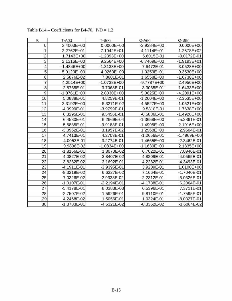
B-15


K T-A(k) T-B(k) Q-A(k) Q-B(k)0 2.4003E+00 0.0000E+00 -3.9384E+00 0.0000E+001 2.2762E+01 -7.1042E+01 -4.1114E+01 1.2578E+022 1.7143E+00 -1.2393E+00 5.6015E-01 -3.0172E-013 2.1316E+00 9.2564E+00 -6.7469E+00 -1.9193E+014 -1.4846E+00 -1.3138E+00 7.6472E-01 3.0528E+005 -5.9120E+00 4.9260E+00 1.0259E+01 -9.3530E+006 2.5876E-02 7.8601E-01 1.6558E+00 -1.6738E+007 4.2514E+00 -1.0738E+00 -9.7787E+00 2.4956E+008 -2.8765E-01 -3.7068E-01 3.3065E-01 1.6433E+009 -1.8761E+00 2.8030E+00 5.0625E+00 -4.2091E+00

10 5.0888E-01 4.8259E-01 -1.2604E+00 -2.3535E+0011 2.3192E+00 -5.3271E-02 -4.5527E+00 -1.0521E+0012 -4.0999E-01 -3.9799E-01 9.5818E-01 1.7638E+0013 6.3295E-01 9.5456E-01 -6.5886E-01 -1.4926E+0014 6.4530E-01 6.2669E-04 -1.3658E+00 -5.2861E-0115 5.5885E-01 -9.9188E-01 -1.4995E+00 2.1916E+0016 -3.0962E-01 3.1957E-02 1.2968E+00 2.9604E-0117 4.7413E-01 4.2703E-01 -1.2656E-01 -1.4969E+0018 4.0053E-01 -3.2774E-01 -1.4665E+00 -2.3462E-0119 9.9838E-02 -1.0834E+00 -1.1630E+00 2.1835E+0020 -1.8166E-01 1.8070E-02 6.7022E-01 7.0940E-0121 4.0827E-02 3.8407E-02 4.8209E-01 -4.0565E-0122 3.8262E-02 -3.1692E-01 -4.2282E-01 4.3493E-0123 -4.1911E-01 -3.9395E-01 3.9209E-01 1.0100E+0024 -8.3219E-02 6.6227E-02 7.1664E-01 -1.7040E-0125 7.0326E-02 -2.9338E-02 -2.2312E-01 -5.0326E-0126 -1.0107E-01 -2.2194E-01 -4.1788E-01 6.2064E-0127 -5.4178E-01 8.0383E-03 6.5396E-01 7.3711E-0128 -2.7507E-02 1.5926E-01 9.8110E-01 -1.7595E-0129 4.2468E-02 1.5056E-01 1.0324E-01 -8.0327E-0130 -1.3783E-01 -4.5321E-02 -8.3362E-02 -3.6084E-02

B-16


K T-A(k) T-B(k) Q-A(k) Q-B(k)0 1.8891E+00 0.0000E+00 -6.2730E+00 0.0000E+001 2.8033E+01 -6.5683E+01 -5.9067E+01 1.3718E+022 1.8860E+00 -2.3066E-01 3.4811E+00 -6.0201E-023 5.9973E-01 7.4446E+00 -4.3989E+00 -2.0555E+014 -1.0858E+00 -1.2398E+00 -4.0520E-01 3.3632E+005 -6.4362E+00 4.7921E+00 1.1843E+01 -8.9586E+006 -1.5631E-01 7.1695E-01 3.0860E+00 -2.6638E+007 5.0311E+00 3.4276E-02 -1.3137E+01 -9.8190E-018 -6.3924E-02 -2.9434E-01 -1.4057E+00 2.2511E+009 -2.0315E+00 2.0101E+00 5.6834E+00 -8.7269E-01

10 6.0866E-01 2.7097E-01 2.6129E-01 -3.1696E+0011 1.8917E+00 1.6480E-01 -4.5913E+00 -3.3156E+0012 -4.1935E-01 -1.7983E-01 -5.8107E-01 2.1286E+0013 6.7181E-01 1.0989E+00 -1.2353E-01 -1.0776E+0014 6.4230E-01 -1.6326E-01 -1.6486E+00 -1.3561E+0015 7.2715E-01 -1.3135E+00 -4.3524E+00 2.0842E+0016 -1.7483E-01 -3.0559E-03 9.5606E-01 2.0193E+0017 1.7548E-01 4.6619E-01 2.0063E+00 3.3011E-0118 3.5480E-01 -3.9988E-01 -6.7764E-01 -1.0371E+0019 7.9700E-02 -7.4616E-01 -2.0860E+00 1.3432E+0020 -9.9109E-02 1.8552E-02 1.0021E-01 1.2629E+0021 2.2019E-01 -9.1938E-02 1.4317E+00 3.9292E-0122 -4.7530E-02 -4.1697E-01 -4.0246E-01 -1.5316E-0123 -5.2461E-01 -3.0539E-01 -3.4768E-01 1.2626E+0024 5.3469E-02 1.4211E-01 1.1234E+00 1.1060E+0025 9.9510E-02 6.3486E-02 1.8220E+00 -7.6676E-0126 -1.6191E-01 -2.7402E-01 -3.4224E-01 -7.1063E-0127 -3.4163E-01 9.2732E-03 -6.7856E-01 7.8099E-0228 2.5212E-02 1.1064E-01 8.9990E-01 7.0479E-0129 4.6286E-03 -1.7769E-02 8.4620E-01 -6.6394E-0130 -2.0432E-01 6.4717E-03 -8.4567E-02 -6.1846E-01

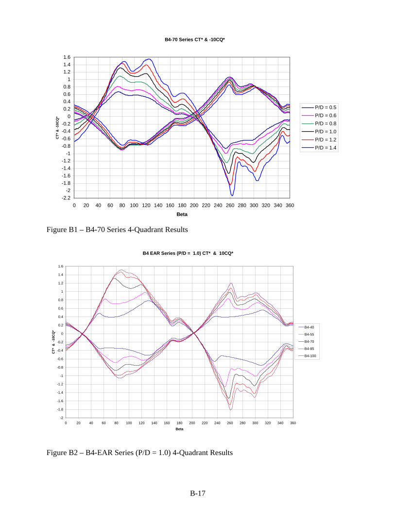
B-17

Figure B1 – B4-70 Series 4-Quadrant Results Figure B2 – B4-EAR Series (P/D = 1.0) 4-Quadrant Results

B4-70 Series CT* & -10CQ*

-2.2-2

-1.8-1.6-1.4-1.2

-1-0.8-0.6-0.4-0.2

00.20.40.60.8

11.21.41.6

0 20 40 60 80 100 120 140 160 180 200 220 240 260 280 300 320 340 360

Beta

CT*

& -1

0CQ

*

P/D = 0.5P/D = 0.6P/D = 0.8P/D = 1.0P/D = 1.2P/D = 1.4

B4 EAR Series (P/D = 1.0) CT* & 10CQ*

-2

-1.8

-1.6

-1.4

-1.2

-1

-0.8

-0.6

-0.4

-0.2

0

0.2

0.4

0.6

0.8

1

1.2

1.4

1.6

0 20 40 60 80 100 120 140 160 180 200 220 240 260 280 300 320 340 360

Beta

CT*

& -

10C

Q*

B4-40

B4-55

B4-70

B4-85

B4-100

B-18

B-(Blade No.) Series CT* & -10CQ*

-1.6

-1.4

-1.2

-1

-0.8

-0.6

-0.4

-0.2

0

0.2

0.4

0.6

0.8

1

1.2

1.4

0 20 40 60 80 100 120 140 160 180 200 220 240 260 280 300 320 340 360

Beta

CT*

& -1

0CQ

* B3-65B4-70B5-75B6-80B7-85

Figure B3 – B-(Blade No.) Series (P/D = 1.0 and EAR ≈ 0.7)

C-1

Appendix C

Intelligent Calculation of Equations (ICE)

C-2

The Intelligent Calculation of Equations (ICE) is built around the executable code (ICE.exe) that automatically solves nonlinear equation systems. In addition, a linearized solution, to the extent possible, is determined. The ICE routines work on a user defined input data set comprised of independent variables (inputs) and dependent variables (outputs). All of the required input information about the data set and the options to ICE to use are defined in the input file (ICE_setup.fi).

The ICE package, ICE.exe and ICE_setup.fi, automatically solve for an optimal nonlinear solution to the data set using feedforward neural networks. The code can also determine the critical independent variables required for the solution. Any nonlinear system where the independent variables are not known can be solved by providing a broad estimate, best guess at the relevant inputs to the model. The code, in an automated fashion, then outputs both a fully nonlinear model of the system as well as a set of linearized equations.

The data set should be an ASCII file that is space delimited, tab delimited or comma

delimited. The number of rows and columns are specified in the setup file. All of the input/output (I/O) data is then contained in columns and rows. Each column should correspond to a single variable and each row of data should correspond to a specific set of I/O conditions. All data, whether it is used or not, can be included in a single data set; specific columns for the I/O are defined in the input file. As such, the data set can contain many more inputs and outputs than may actually be specified as part of any given solution. The executable assumes a maximum of 160 inputs, 20 outputs and 10,000 I/O pairings. Applied Simulation Technologies can increase these limits if it is necessary.

A note on the data: the data set should have all variables in either dimensional or

nondimensional form as required, or needed, for the solution of interest. For temporal data some effort should be made to utilize a sampling frequency that is representative of the underlying frequency content of the problem (data). A sampling frequency of two to five times the Nyquist criterion is usually reasonable. On the other hand, having data sampled at 100 Hz for a 1 Hz problem, for example, will typically yield a less than optimal solution. It is recommended that you decimate the data sets accordingly prior to running the ICE solution. You can of course, try the solution at any sampling rate for which the data exists. ASCII file format: HI1, HI2, HIN, HO1, HO2, HOM (Optional Header Row) I1, I2, IN, O1, O2, OM . . . I1, I2, IN, O1, O2, OM

The solutions can be of the form single-input-single-output (SISO), multiple-input-

multiple-output (MIMO), or multiple-input-single-output (MISO). MISO solutions will yield the

C-3

best result, so for cases with multiple outputs it may be advantageous to develop multiple solutions, one for each output. The final solution, as well as the accuracy, is determined using 1/3 data pts as a novel, unused, test group.

In addition to the flexibility of the input file there are several important options to ICE

that greatly add to its utility. The user can:

1. Have ICE determine the neural network (NN) architecture (the default), or can specify the architecture;

2. Have ICE use its standard learning algorithm, or specify a modified algorithm that is better when the input data set has many values very near zero;

3. Have ICE determine the single “best” solution, or specify a number of solutions (up to 50) so that the final solution is an average of these multiple solutions;

4. Have ICE determine a solution that is only good for interpolation, or specify the degree of extrapolation allowed; and,

5. Have ICE adaptively remove unnecessary inputs and update the NN inputs and architecture accordingly, or specify that all inputs must be used.

C-4


D-1

APPENDIX D

Derivation of Matching Polynomial Computation

D-2

Matching Polynomial Computation

As described previously, separate feedforward neural networks (FFNN) were implemented in four overlapping regions of the range of the advance angle, β , in order to maximize prediction quality. The penalty incurred with such an approach is that there are, inevitably, discontinuities at the boundaries when moving from one FFNN prediction to another. An example is illustrated in Figure D1. Although these breaks are typically small, two procedures were developed to smoothly fit a polynomial from one prediction to the other, thereby ensuring continuity. One procedure matches the slopes and the other matches both slope and curvature.

Figure D1 - Plot of Thrust Coefficient vs. Beta Showing Mismatched Predictions at One of the Boundaries

Each FFNN prediction is a thrust coefficient or torque coefficient function of the form ( )β,,, ZEARDPCC TT = or ( )β,,, ZEARDPCC QQ = , where DP is the pitch to diameter ratio, EAR is the

expanded area ratio, Z is the number of blades and β is the advance angle. A given curve as shown in Fig. D1 represents the variation ( )βTT CC = for fixed values of DP , EAR and Z. To simplify the notation, the FFNN prediction to the left of the boundary will be referred to as )(xg , the one on the right will be )(xh , and the matching polynomial will be referred to as )(xf .

Matching Slopes

The simpler procedure begins by defining a closed interval ],[ ba , which contains the boundary as shown in Figure D1. This interval defines the domain of the matching polynomial. The polynomial will be required to match the function values, )(ag and )(bh , as well as the slopes, )(ag′ and )(bh′ , at the endpoints of the interval. To find a unique polynomial that will match these four conditions requires that it have four adjustable coefficients and be of the form

33

2210)( xcxcxccxf +++= . (1)

The matching conditions then become

-1.3

-1.1

-0.9

-0.7

-0.5

-0.3

-0.1

0.1

0.3

0.5

200 210 220 230 240 250 260

Beta

CT

a b

g(x)h(x)

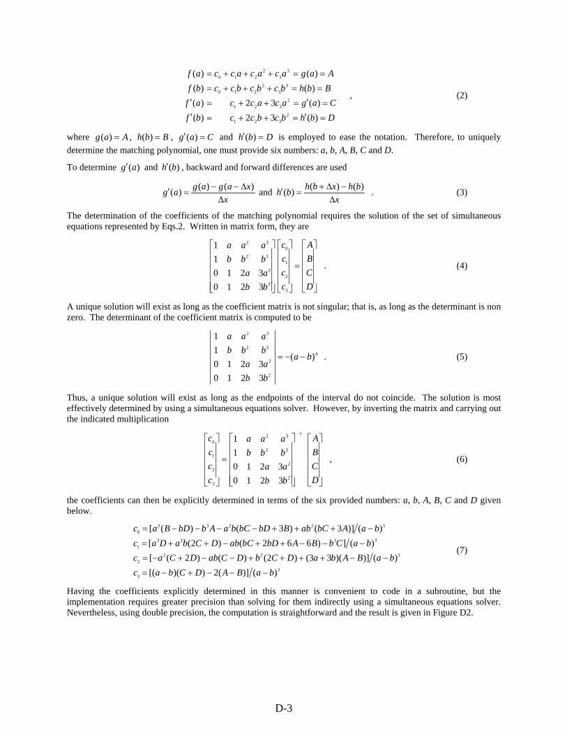
D-3

DbhbcbccbfCagacaccaf

BbhbcbcbccbfAagacacaccaf

=′=++=′=′=++=′

==+++=

==+++=

)(32)()(32)(

)()()()(

2321

2321

33

2210

33

2210

, (2)

where Aag =)( , Bbh =)( , Cag =′ )( and Dbh =′ )( is employed to ease the notation. Therefore, to uniquely determine the matching polynomial, one must provide six numbers: a, b, A, B, C and D.

To determine )(ag′ and )(bh′ , backward and forward differences are used

x

bhxbhbhx

xagagag∆

−∆+=′

∆∆−−

=′ )()()( and )()()( . (3)

The determination of the coefficients of the matching polynomial requires the solution of the set of simultaneous equations represented by Eqs.2. Written in matrix form, they are

⎥⎥⎥⎥

⎦

⎤

⎢⎢⎢⎢

⎣

⎡

=

⎥⎥⎥⎥

⎦

⎤

⎢⎢⎢⎢

⎣

⎡

⎥⎥⎥⎥⎥

⎦

⎤

⎢⎢⎢⎢⎢

⎣

⎡

DCBA

cccc

bbaabbbaaa

3

2

1

0

2

2

32

32

32103210

11

. (4)

A unique solution will exist as long as the coefficient matrix is not singular; that is, as long as the determinant is non zero. The determinant of the coefficient matrix is computed to be

4

2

2

32

32

)(

32103210

11

ba

bbaabbbaaa

−−= . (5)

Thus, a unique solution will exist as long as the endpoints of the interval do not coincide. The solution is most effectively determined by using a simultaneous equations solver. However, by inverting the matrix and carrying out the indicated multiplication

⎥⎥⎥⎥

⎦

⎤

⎢⎢⎢⎢

⎣

⎡

⎥⎥⎥⎥⎥

⎦

⎤

⎢⎢⎢⎢⎢

⎣

⎡

=

⎥⎥⎥⎥

⎦

⎤

⎢⎢⎢⎢

⎣

⎡−

DCBA

bbaabbbaaa

cccc

1

2

2

32

32

3

2

1

0

32103210

11

, (6)

the coefficients can then be explicitly determined in terms of the six provided numbers: a, b, A, B, C and D given below.

33

3222

33231

322330

)()](2))([()()])(33()2()()2([

)(])662()2([)()]3()3()([

baBADCbacbaBAbaDCbDCabDCac

baCbBAbDbCabDCbaDacbaAbCabBbDbCbaAbbDBac

−−−+−=

−−++++−−+−=

−−−++−++=

−+++−−−−=

(7)

Having the coefficients explicitly determined in this manner is convenient to code in a subroutine, but the implementation requires greater precision than solving for them indirectly using a simultaneous equations solver. Nevertheless, using double precision, the computation is straightforward and the result is given in Figure D2.

D-4

Matching Curvatures

A more visually appealing solution results when one requires that the matching polynomial satisfy not only function values and slopes at the endpoints of the interval, but also second derivatives (curvatures) as well. Specifically, the polynomial will be required to match the function values, )(ag and )(bh , the slopes, )(ag′ and

)(bh′ , and the curvatures, )(ag ′′ and )(bh ′′ , at the endpoints of the interval. To find a unique polynomial that will match these six conditions requires that it have six adjustable coefficients and be of the form

55

44

33

2210)( xcxcxcxcxccxf +++++= . (8)

The matching conditions then become

FbhbcbcbccbfEagacacaccafDbhbcbcbcbccbfCagacacacaccaf

BbhbcbcbcbcbccbfAagacacacacaccaf

=′′=+++=′′=′′=+++=′′=′=++++=′=′=++++=′

==+++++=

==+++++=

)(201262)()(201262)()(5432)()(5432)(

)()()()(

35

2432

35

2432

45

34

2321

45

34

2321

55

44

33

2210

55

44

33

2210

, (9)

where Aag =)( , Bbh =)( , Cag =′ )( , Dbh =′ )( , Eag =′′ )( and Fbh =′′ )( is employed to ease the notation. Therefore, to uniquely determine the matching polynomial, the user must provide eight numbers: a, b, A, B, C, D, E and F.

To determine )(ag′ , )(bh′ , )(ag ′′ and )(bh ′′ , backward and forward differences are used

( ) ( )22

)()(2)2()( and )2()(2)()(

)()()( and )()()(

xbhxbhxbhbh

xxagxagagag

xbhxbhbh

xxagagag

∆+∆+−∆+

=′′∆

∆−+∆−−=′′

∆−∆+

=′∆

∆−−=′

. (10)

The simultaneous equations are represented in matrix form as

⎥⎥⎥⎥⎥⎥⎥⎥

⎦

⎤

⎢⎢⎢⎢⎢⎢⎢⎢

⎣

⎡

=

⎥⎥⎥⎥⎥⎥⎥⎥

⎦

⎤

⎢⎢⎢⎢⎢⎢⎢⎢

⎣

⎡

⎥⎥⎥⎥⎥⎥⎥⎥

⎦

⎤

⎢⎢⎢⎢⎢⎢⎢⎢

⎣

⎡

FEDCBA

cccccc

bbbaaa

bbbbaaaabbbbbaaaaa

5

4

3

2

1

0

32

32

432

432

5432

5432

2012620020126200543210543210

11

. (11)

The determinant of the coefficient matrix is computed to be

9

32

32

432

432

5432

5432

)(4

2012620020126200543210543210

11

ba

bbbaaa

bbbbaaaabbbbbaaaaa

−= . (12)

Again, one sees that a unique solution will exist as long as the endpoints of the interval do not coincide. Inverting the matrix and carrying out the indicated multiplication

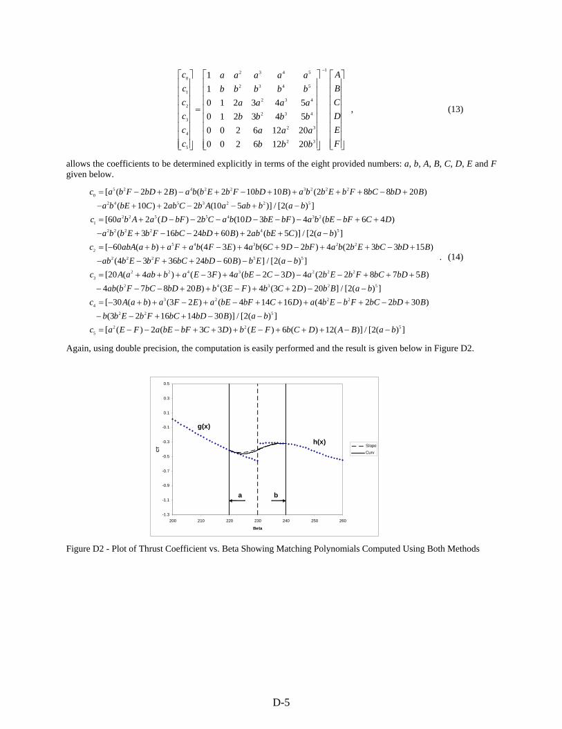
D-5

⎥⎥⎥⎥⎥⎥⎥⎥

⎦

⎤

⎢⎢⎢⎢⎢⎢⎢⎢

⎣

⎡

⎥⎥⎥⎥⎥⎥⎥⎥

⎦

⎤

⎢⎢⎢⎢⎢⎢⎢⎢

⎣

⎡

=

⎥⎥⎥⎥⎥⎥⎥⎥

⎦

⎤

⎢⎢⎢⎢⎢⎢⎢⎢

⎣

⎡−

FEDCBA

bbbaaa

bbbbaaaabbbbbaaaaa

cccccc

1

32

32

432

432

5432

5432

5

4

3

2

1

0

2012620020126200543210543210

11

, (13)

allows the coefficients to be determined explicitly in terms of the eight provided numbers: a, b, A, B, C, D, E and F given below.

])(2[/)](12)(6)()33(2)([])(2[/)]30141623(

)30224()16144()23()(30[])(2[/]20)23(4)3()2087(4

)57822(4)32(4)3()4(20[])(2[/])60243634(

)15332(4)296(4)34()(60[])(2[/)]5(2)6024163(

)46(4)310(2)(260[])(2[/)]510(22)10(

)20882()10102()22([

5225

522

22234

52342

22234223

55222

223452

542222

23455221

5223542

2223224250

baBADCbFEbDCbFbEaFEacbaBbDbCFbEbb

BbDbCFbEbaDCbFbEaEFabaAcbaBbDCbFEbBbDbCFbab

BbDbCFbEbaDCbEaFEababaAcbaEbBbDbCFbEbab

BbDbCEbbabFDCbaEFbaFabaabAcbaCbEabBbDbCFbEbba

DCbFbEbabFbEDbaCbbFDaAbacbababaAbCabCbEba

BbDbCFbEbbaBbDFbEbbaBbDFbac

−−+++−+++−−−=

−−++−−

+−+−+++−+−++−=

−−++−++−−−

+++−−−−+−+++=

−−−++−−

+−++−++−+++−=

−+++−−+−

++−−−−−−−+=

−+−−++−

+−++++−+−+−=

. (14)

Again, using double precision, the computation is easily performed and the result is given below in Figure D2.

Figure D2 - Plot of Thrust Coefficient vs. Beta Showing Matching Polynomials Computed Using Both Methods

-1.3

-1.1

-0.9

-0.7

-0.5

-0.3

-0.1

0.1

0.3

0.5

200 210 220 230 240 250 260

Beta

CT

SlopeCurv

a b

g(x)

h(x)

D-6


E-1

APPENDIX E

Summary of Coefficients and Results For

Nozzle 19a with Ka4-70 From

“Wake Adapted Ducted Propellers” (Reference 16)

E-2

The open-water characteristics of the Wageningen Nozzle 19a with the Ka4-70 series of propellers were faired by means of harmonic analyses, and the results are presented in Reference 16. The resulting harmonic analysis coefficients are presented in Table E1 and are in the form of:

( ) ( ){ }∑=

+=30

0

* sin)(cos)(100

1k

T kkBkkAC ββ

( ) ( ){ }∑=

β+β=30

0k

*Tn ksin)k(Bkcos)k(A

1001C

( ) ( ){ }∑=

+−

=30

0

* sin)(cos)(1000

1k

Q kkBkkAC ββ .

Four quadrant plots generated from these coefficients are presented in Figure E1.

E-3

Table E1 – Coefficients for Nozzle 19a with Ka4-70

K ACT BCT ACTn BCTn ACQ BCQ0 -1.4825E-01 0.0000E+00 -1.4276E-01 0.0000E+00 1.7084E-02 0.0000E+001 8.4697E-02 -1.0838E+00 -5.5945E-03 -2.1875E-01 1.0550E-01 -7.8070E-012 1.6700E-01 -1.8023E-02 1.5519E-01 1.0114E-02 -2.7380E-02 3.8134E-023 9.6610E-04 1.1825E-01 1.5915E-02 4.7120E-02 -1.1827E-02 7.4292E-024 1.4754E-02 -7.0713E-03 6.6633E-03 -5.8914E-04 2.8671E-02 -1.3568E-025 -1.1806E-02 6.2894E-02 8.9343E-04 -1.2958E-03 4.2504E-03 6.6595E-026 -1.4888E-02 1.1519E-02 -3.8876E-03 -2.0824E-03 -7.8835E-03 1.0330E-027 7.3311E-03 1.7070E-03 1.0976E-02 5.2475E-03 -7.0981E-03 -1.7885E-028 7.5022E-03 2.2990E-03 3.1959E-03 -1.5428E-03 7.6691E-03 -3.6187E-039 -1.5128E-02 1.3458E-02 1.4201E-03 2.3580E-03 -1.2506E-02 1.0015E-0210 3.3002E-03 5.4810E-04 1.3507E-03 2.3491E-04 -7.0343E-03 5.5926E-0311 3.1416E-03 4.2076E-03 5.0526E-03 -2.6868E-03 -1.0254E-02 6.9688E-0312 -2.1144E-03 -5.7232E-03 -9.0855E-04 -4.5635E-03 2.5186E-03 -4.7676E-0313 2.9438E-03 7.4689E-03 4.2758E-05 -4.4554E-05 9.6613E-03 8.8889E-0314 3.3857E-04 -8.4815E-05 4.2084E-04 -1.8564E-05 1.4934E-03 4.9081E-0315 4.1236E-03 -1.3374E-03 2.0269E-03 -8.0547E-04 -2.8323E-03 -5.8150E-0516 1.6259E-03 -9.1934E-04 -7.9748E-04 -1.0170E-03 -3.0360E-03 5.2044E-0317 1.2759E-03 2.7412E-03 9.7452E-04 -4.6721E-05 2.0889E-03 1.2522E-0318 2.0647E-03 -1.0198E-03 4.8897E-04 -1.7088E-04 3.1929E-03 3.3190E-0319 3.4157E-03 1.9845E-03 8.4347E-04 -6.0673E-04 -9.1635E-04 5.2446E-0320 -5.8703E-04 -1.3980E-03 -3.9298E-04 -3.6317E-04 -2.3922E-03 -2.0591E-03

P/D=0.6

K ACT BCT ACTn BCTn ACQ BCQ0 -1.3080E-01 0.0000E+00 -1.2764E-01 0.0000E+00 1.9368E-02 0.0000E+001 1.0985E-01 -1.0708E+00 6.8679E-04 -2.4100E-01 1.7050E-01 -9.9912E-012 1.5810E-01 2.4163E-02 1.4639E-01 1.8919E-02 -1.1901E-02 3.1924E-023 1.8367E-02 1.2784E-01 2.3195E-02 5.5513E-02 -2.5601E-03 8.1384E-024 1.6168E-02 -1.4064E-03 1.0292E-02 -1.2453E-03 1.7763E-02 -3.5096E-045 -3.7402E-03 7.6213E-02 8.6651E-03 -1.4748E-03 8.2085E-03 1.0631E-016 -1.1736E-02 1.3259E-02 -3.9124E-03 -2.1899E-03 -3.4336E-03 1.5116E-027 2.5483E-03 -4.2300E-03 1.5984E-02 5.6694E-03 -2.4534E-02 -2.7045E-028 1.2350E-03 -2.6246E-03 4.6295E-03 -4.9911E-03 -1.0289E-03 -5.9389E-039 -2.0772E-03 1.6328E-02 6.8371E-04 1.3631E-03 -7.4938E-03 1.1085E-0210 6.9749E-03 -3.3979E-04 1.6740E-03 1.2877E-03 1.5444E-03 8.3787E-0311 5.9838E-03 2.3506E-03 8.3495E-03 -3.5176E-03 -1.4173E-02 1.5192E-0212 -1.4599E-03 -6.9497E-03 -7.7063E-04 -5.5571E-03 -2.8034E-03 -5.1507E-0313 8.3533E-03 6.1925E-03 1.4936E-03 3.1438E-04 1.4246E-02 1.4836E-0214 1.1093E-03 3.5046E-04 1.1017E-03 -1.1179E-03 3.4663E-03 2.5041E-0315 4.1885E-03 -1.1571E-03 1.6804E-03 -2.4577E-03 2.0764E-03 -7.8615E-0416 -1.2438E-04 -3.2566E-04 -1.0338E-03 -5.5484E-04 -2.9424E-03 -2.4526E-0317 3.8034E-03 6.3420E-04 2.2409E-03 1.0968E-04 3.0149E-03 -3.2187E-0418 9.0073E-04 -2.2749E-03 1.1000E-03 -7.3945E-04 2.7714E-03 -4.8551E-0419 3.1147E-03 -3.6805E-04 4.8406E-04 -1.5400E-03 1.8423E-04 3.5455E-0320 -1.0633E-04 -1.2350E-03 -3.3008E-04 2.2408E-04 -8.1634E-05 -3.4936E-04

P/D=0.8

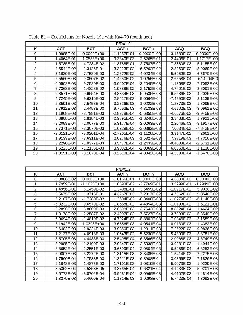
E-4

Table E1 – Coefficients for Nozzle 19a with Ka4-70 (continued)

K ACT BCT ACTn BCTn ACQ BCQ0 -1.0985E-01 0.0000E+00 -1.1257E-01 0.0000E+00 3.1589E-02 0.0000E+001 1.4064E-01 -1.0583E+00 9.3340E-03 -2.6265E-01 2.4406E-01 -1.1717E+002 1.5785E-01 4.7284E-02 1.3788E-01 2.7587E-02 -7.3880E-03 5.1155E-023 4.5544E-02 1.3126E-01 3.3223E-02 6.5262E-02 2.8260E-02 8.9069E-024 5.1639E-03 -7.7539E-03 1.2672E-02 -4.0234E-03 -5.5959E-03 -6.5670E-035 -2.5560E-03 9.3507E-02 1.4250E-02 1.0255E-03 2.6558E-04 +.14204E 06 -6.0502E-03 9.2520E-03 -3.0407E-04 -3.2045E-03 1.1368E-02 7.7052E-037 6.7368E-03 -1.4828E-02 1.9888E-02 -2.1752E-03 -4.7401E-02 -3.6091E-028 6.8571E-03 -9.6554E-03 4.8334E-03 -5.9535E-03 -6.5686E-03 4.2036E-039 4.7245E-03 9.6216E-03 2.8427E-03 9.0664E-04 -7.4990E-03 2.1139E-0310 2.3591E-03 -7.5453E-04 3.2326E-03 -1.0222E-03 1.2873E-03 1.3095E-0211 8.7912E-03 2.4453E-03 9.7693E-03 -4.8133E-03 4.6502E-03 3.0961E-0212 1.1968E-03 -8.7981E-03 -2.8378E-04 -5.6355E-03 -4.6676E-03 -9.9459E-0313 8.3808E-03 1.8184E-03 2.9395E-03 -1.8248E-03 3.3438E-03 1.7921E-0214 -8.2098E-04 -2.0077E-03 5.3177E-04 -2.0263E-03 2.2046E-03 -8.1917E-0315 2.7371E-03 -3.3070E-03 1.6229E-03 -3.0382E-03 7.0034E-03 -7.8428E-0416 -2.6121E-04 -7.9201E-04 -2.7265E-04 -1.1128E-03 3.9147E-02 7.2661E-0317 1.9133E-03 -3.6311E-04 2.0276E-03 -1.5327E-03 7.3719E-03 -4.7316E-0318 3.2290E-04 -1.9377E-03 3.5477E-04 -1.2433E-03 -9.4083E-04 -2.5731E-0319 1.5223E-03 -1.2135E-03 3.9082E-04 -2.0069E-03 6.0560E-03 1.1136E-0320 -1.0151E-03 -3.1678E-04 -9.2513E-04 -4.8842E-04 -4.2390E-04 -1.5470E-03

P/D=1.0

K ACT BCT ACTn BCTn ACQ BCQ0 -9.0888E-02 0.0000E+00 -1.0166E-01 0.0000E+00 4.3800E-02 0.0000E+001 1.7959E-01 -1.1026E+00 1.8593E-02 -2.7769E-01 3.5299E-01 -1.2949E+002 1.4956E-01 6.1459E-02 1.3408E-01 3.5459E-02 -1.0917E-02 5.9030E-023 6.5675E-02 1.3715E-01 4.3767E-02 7.2317E-02 4.7062E-02 9.3540E-024 5.2107E-03 -1.7280E-02 1.3604E-02 -8.3408E-03 -1.0779E-02 -6.1148E-035 -6.8232E-03 9.6579E-02 1.8658E-02 4.4854E-03 -1.0193E-02 1.6121E-016 -6.2896E-03 5.8809E-03 2.6598E-03 -3.7642E-03 -8.8824E-04 1.4624E-027 1.8178E-02 -2.2587E-02 2.4907E-02 7.5727E-04 -3.7893E-02 -5.3549E-028 6.0694E-03 -1.4819E-02 4.7924E-03 -8.8802E-03 -7.0346E-03 -3.1589E-039 6.1942E-03 -1.0398E+00 3.6556E-03 4.0541E-04 -8.0130E-03 1.4382E-0210 2.6482E-03 -2.9324E-03 3.9850E-03 -1.2811E-03 7.2622E-03 9.9836E-0311 1.2137E-02 4.0913E-03 1.0643E-02 -5.5230E-03 -5.4390E-03 3.8781E-0212 -3.5705E-03 -4.4436E-03 2.5495E-04 -6.3566E-03 -2.0068E-03 -4.6749E-0313 3.2985E-03 -1.2190E-03 2.9347E-03 -2.5338E-03 3.9281E-03 1.4944E-0214 -8.8652E-04 -2.2551E-03 3.6599E-04 -2.0504E-03 -6.5256E-04 -6.3253E-0315 6.9807E-03 -3.2272E-03 1.3115E-03 -3.8485E-03 1.5414E-02 2.2275E-0316 -1.7560E-04 1.7533E-03 -1.3511E-03 -6.3908E-04 3.0356E-03 7.1826E-0317 2.1643E-03 1.4875E-03 1.7101E-03 -1.0819E-03 5.9073E-03 1.0229E-0318 3.5362E-04 4.5353E-05 3.3765E-04 -9.6321E-04 4.1433E-03 -5.9201E-0319 2.5772E-03 -8.8702E-04 -3.9681E-04 -2.0969E-03 4.6102E-03 -1.4814E-0320 -1.8279E-03 -9.4609E-04 -1.1814E-03 -1.9298E-04 -5.7423E-04 -4.3092E-03

P/D=1.2

E-5

Table E1 – Coefficients for Nozzle 19a with Ka4-70 (continued)

K ACT BCT ACTn BCTn ACQ BCQ0 -7.3487E-02 0.0000E+00 -8.6955E-02 0.0000E+00 7.3202E-02 0.0000E+001 2.2861E-01 -9.8101E-01 3.0046E-02 -2.9799E-01 +.47301E 0 -1.4062E+002 1.4853E-01 7.1510E-02 1.2651E-01 4.3403E-02 -3.3300E-02 7.1683E-023 7.5328E-02 1.4217E-01 5.5034E-02 8.3309E-02 6.2786E-02 1.1449E-014 3.4084E-03 -2.2675E-02 1.9376E-02 -1.4571E-02 -1.9511E-02 -1.3400E-025 -1.1643E-03 9.1082E-02 2.2082E-02 4.3398E-03 -2.7569E-02 1.7547E-016 1.8576E-04 -4.0283E-03 7.6282E-03 -3.9256E-03 -3.8296E-03 2.5715E-027 2.6970E-02 -2.2759E-02 3.1821E-02 -2.3504E-03 -2.3310E-02 -5.4967E-028 2.0616E-03 -1.6727E-02 5.1835E-03 -1.3633E-02 -8.4525E-03 -1.2576E-029 7.8666E-03 8.6970E-03 3.8898E-03 -1.4000E-03 -4.8956E-03 1.3084E-0210 4.6912E-03 -4.7515E-03 4.9300E-03 -2.8212E-03 4.8544E-03 1.0733E-0211 1.4771E-02 2.2828E-03 1.0731E-02 -7.7360E-03 -7.1945E-03 4.4142E-0212 -7.5056E-03 -4.9383E-03 1.1388E-03 -6.8665E-03 -5.3186E-03 -1.0945E-0313 1.4983E-03 -2.5924E-03 3.1378E-03 -4.2392E-03 1.3281E-03 1.2209E-0214 2.4058E-03 -2.5143E-03 -8.2607E-04 -3.3252E-03 6.8695E-03 -1.4074E-0315 5.5647E-03 -3.3659E-03 -1.7537E-05 -4.5496E-03 1.8071E-02 1.7837E-0316 -3.8178E-03 2.8153E-03 -3.6227E-03 -1.2282E-03 -1.5725E-03 3.7948E-0317 2.6704E-03 -2.2162E-04 -2.2400E-04 -1.5759E-03 1.1527E-02 4.9971E-0318 1.5745E-03 -5.3749E-04 -5.8416E-04 -7.7655E-07 1.0168E-02 -4.2398E-0319 2.4500E-04 -3.5190E-03 -1.2806E-03 -1.7787E-03 8.1504E-04 -7.7298E-0320 -4.2370E-05 -4.2846E-04 -1.9870E-03 4.9570E-04 1.4051E-03 -3.4485E-03

P/D=1.4

E-6

Figure E1 – Nozzle 19a with Ka4-70 4-Quadrant Results

-1.8

-1.6

-1.4

-1.2

-1

-0.8

-0.6

-0.4

-0.2

0

0.2

0.4

0.6

0.8

1

1.2

1.4

1.6

0 20 40 60 80 100 120 140 160 180 200 220 240 260 280 300 320 340 360

Beta

CT*

CTn

* -1

0CQ

*

P/D=0.6P/D=0.8P/D=1.0P/D=1.2P/D=1.4

Ct*

Ctn*

-10Cq*

F-1

APPENDIX F

Summary of Coefficients and Results From For

Nozzle 37 with Ka4-70 “Wake Adapted Ducted Propellers”

(Reference 16)

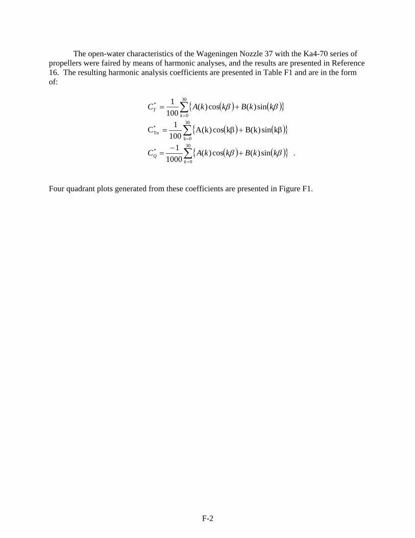
F-2

The open-water characteristics of the Wageningen Nozzle 37 with the Ka4-70 series of propellers were faired by means of harmonic analyses, and the results are presented in Reference 16. The resulting harmonic analysis coefficients are presented in Table F1 and are in the form of:

( ) ( ){ }∑=

+=30

0

* sin)(cos)(100

1k

T kkBkkAC ββ

( ) ( ){ }∑=

β+β=30

0k

*Tn ksin)k(Bkcos)k(A

1001C

( ) ( ){ }∑=

+−

=30

0

* sin)(cos)(1000

1k

Q kkBkkAC ββ .

Four quadrant plots generated from these coefficients are presented in Figure F1.

F-3

Table F1 – Coefficients for Nozzle 37 with Ka4-70

K ACT BCT ACTn BCTn ACQ BCQ0 -7.8522E-02 0.0000E+00 -7.5854E-02 0.0000E+00 1.4884E-02 0.0000E+001 9.1962E-02 -1.2241E+00 9.1152E-03 -3.4397E-01 1.0044E-01 -7.9096E-012 9.6733E-02 -1.0805E-02 8.5316E-02 -6.0863E-03 -2.5182E-02 1.2206E-023 -1.4657E-03 1.6207E-01 4.7203E-03 8.2506E-02 -1.0918E-02 9.0718E-024 1.0810E-02 1.0642E-03 3.1838E-03 5.1816E-03 2.7502E-02 7.2669E-035 -2.0708E-02 7.8648E-02 4.5464E-03 9.9282E-03 -2.6072E-03 5.7653E-026 -8.0316E-03 1.4098E-02 3.1828E-03 5.9292E-04 -1.1409E-02 1.1032E-047 1.1052E-02 -1.1329E-02 9.5481E-03 -1.9148E-03 9.3808E-04 -9.9388E-038 2.1070E-03 -5.2596E-03 -1.9432E-03 -1.7686E-03 8.2783E-03 -2.2892E-039 -1.6466E-02 1.1815E-02 5.8607E-03 -7.8198E-04 -1.7756E-02 5.3796E-0310 8.5238E-04 -2.3771E-03 -1.5047E-03 -3.0445E-03 -4.2598E-03 3.6876E-0311 3.9384E-03 6.4113E-03 3.8003E-03 -2.7783E-03 -4.6664E-03 9.6603E-0312 -3.2905E-03 5.0027E-03 -6.3250E-04 1.7514E-04 1.0278E-03 4.1719E-0413 2.5672E-03 6.0467E-03 1.0102E-03 -6.0004E-04 2.0667E-03 7.2900E-0314 2.4770E-03 -2.8242E-03 -2.8923E-04 -3.2771E-04 1.8501E-03 9.6970E-0415 6.2208E-03 2.0489E-03 2.6588E-03 1.6418E-04 2.6112E-03 8.7227E-0416 3.4143E-04 3.1069E-04 -1.1302E-04 -1.4323E-03 -3.2505E-03 2.1002E-0417 1.9780E-03 6.3925E-04 1.9966E-03 -1.1456E-03 -7.7389E-04 2.8832E-0318 6.0762E-04 -2.2082E-03 -5.6644E-04 -7.4530E-04 1.3220E-03 7.0445E-0419 3.4488E-03 3.0421E-03 9.5964E-04 -8.3559E-04 1.6856E-03 3.9547E-0320 -1.7166E-03 -5.2892E-04 -5.8527E-04 -5.4179E-05 -4.8127E-04 1.7791E-03

P/D=0.6

K ACT BCT ACTn BCTn ACQ BCQ0 -8.1169E-02 0.0000E+00 -8.5104E-02 0.0000E+00 2.0089E-02 0.0000E+001 1.2849E-01 -1.1842E+00 1.5122E-02 -3.3237E-01 1.6636E-01 -9.9219E-012 1.1331E-01 5.8341E-04 1.0325E-01 2.4803E-03 -1.8388E-02 1.2892E-023 1.5131E-02 1.6441E-01 1.5649E-02 8.9761E-02 -1.9051E-02 9.5272E-024 4.1567E-03 6.2103E-03 7.5680E-04 4.5883E-03 1.6808E-02 1.6045E-025 -1.6220E-02 7.6506E-02 9.2408E-03 2.6548E-03 5.2434E-03 9.4354E-026 -1.1305E-02 9.6359E-03 -2.5160E-09 -4.2819E-03 -1.1019E-02 -3.6169E-037 9.3452E-03 -1.8036E-02 1.8041E-02 -2.4385E-03 -2.6942E-02 -2.2539E-028 1.7779E-03 -1.2146E-02 -1.4737E-03 -4.5051E-03 9.4780E-03 -3.0457E-059 -6.2214E-03 9.2879E-03 4.8237E-03 -1.5233E-03 -1.9689E-03 2.1436E-0310 4.6290E-03 4.0488E-03 -9.9338E-04 -1.5358E-03 1.6447E-03 3.7463E-0311 6.9293E-03 7.3891E-03 4.8625E-03 -3.2041E-03 -1.4766E-02 2.1398E-0212 -2.0445E-03 -4.0761E-03 -1.1657E-03 1.7286E-05 -2.2670E-03 1.9168E-0313 5.9366E-03 5.9307E-03 4.3615E-03 -8.0871E-04 9.3023E-03 7.6358E-0314 -4.4055E-04 -2.2663E-03 -3.8004E-04 -2.1661E-03 4.1823E-03 -3.3249E-0315 7.2301E-03 -1.5148E-03 3.2422E-03 -2.1791E-04 7.7675E-03 2.4934E-0316 -5.3198E-04 -1.3262E-04 -3.7155E-04 -7.2641E-04 -1.3283E-03 3.9206E-0417 2.6809E-03 4.0086E-03 2.2704E-03 -1.3466E-03 -9.2032E-04 -8.3670E-0418 -8.5582E-04 -1.1431E-03 -1.1253E-03 -2.3762E-04 2.5952E-04 -3.1653E-0319 3.2728E-03 -2.5883E-03 1.9759E-03 -1.0735E-03 2.3462E-03 4.1032E-0320 -1.1347E-03 -9.3290E-05 -9.6980E-04 -5.7005E-06 6.9823E-04 2.0375E-03

P/D=0.8

F-4

Table F1 – Coefficients for Nozzle 37 with Ka4-70 (continued)

K ACT BCT ACTn BCTn ACQ BCQ0 -7.8681E-02 0.0000E+00 -8.0432E-02 0.0000E+00 3.0767E-02 0.0000E+001 1.7005E-01 -1.1152E+00 2.9904E-02 -3.2774E-01 2.4472E-01 -1.1315E+002 1.2604E-01 2.0371E-02 1.0546E-01 8.1952E-03 -1.1316E-02 3.3712E-023 2.4444E-02 1.5275E-01 2.1277E-02 9.3073E-02 -8.1658E-03 9.0343E-024 -6.9987E-03 2.8881E-03 -1.4818E-03 3.8289E-03 1.6208E-03 1.2113E-025 -5.2998E-03 7.8299E-02 1.5667E-02 2.1950E-04 8.6632E-03 1.2138E-016 -7.7500E-03 1.8865E-03 1.7592E-03 -6.3045E-03 -3.4936E-03 -5.4322E-037 6.7088E-03 -2.4665E-02 2.5671E-02 -2.3125E-03 -4.6075E-02 -3.5712E-028 7.8818E-03 -8.2956E-03 -9.0447E-04 -3.6290E-03 6.6651E-03 6.3862E-039 8.3058E-03 1.5085E-02 8.8204E-03 -9.0853E-04 6.1510E-03 1.4021E-0210 2.0833E-03 1.5879E-03 -1.8008E-03 -1.8997E-03 5.1947E-03 2.8095E-0311 7.2262E-03 9.5129E-03 8.1643E-03 -4.0480E-03 -1.3702E-02 3.2828E-0212 -5.8329E-04 -7.3249E-03 -9.7356E-04 -3.4197E-04 1.2766E-04 -1.9195E-0313 8.8467E-03 3.4931E-03 6.9039E-03 -1.3522E-03 6.1680E-03 8.8817E-0314 -2.9559E-03 -6.3570E-03 -5.6244E-04 -2.2322E-03 1.2713E-03 -7.1309E-0315 1.1530E-02 -2.2474E-03 4.5475E-03 -1.4808E-03 1.4570E-02 3.0977E-0316 -8.3057E-04 2.5069E-03 -3.8196E-04 -1.1481E-03 4.4360E-03 6.4517E-0417 3.1339E-03 -1.2990E-03 3.1160E-03 -2.8678E-03 1.8140E-03 -2.2876E-0318 -1.3290E-03 -4.1905E-04 -1.1878E-03 -2.5410E-04 -4.3127E-03 -9.8748E-0519 3.0666E-03 -2.8288E-03 1.9158E-03 -2.5631E-03 3.8794E-03 1.0718E-0320 -1.3749E-03 -4.5929E-04 -1.3129E-03 2.2029E-05 1.4728E-04 -2.3283E-03

P/D=1.0

K ACT BCT ACTn BCTn ACQ BCQ0 -6.0256E-02 0.0000E+00 -7.2310E-02 0.0000E+00 4.4351E-02 0.0000E+001 2.2360E-01 -1.0687E+00 4.7220E-02 -3.2899E-01 3.4230E-01 -1.2562E+002 1.2353E-01 2.9643E-02 1.0455E-01 1.7983E-02 -1.8087E-02 5.5298E-023 2.4086E-02 1.4275E-01 2.3912E-02 9.3061E-02 3.5568E-03 9.2837E-024 -1.4518E-02 -1.4016E-02 -3.2961E-03 -6.3572E-03 -6.3786E-03 -4.9373E-035 -6.2461E-03 7.3413E-02 2.4863E-02 7.4431E-04 -1.3513E-02 1.4129E-016 -4.3441E-03 7.0950E-04 1.7700E-04 -3.0252E-03 9.4572E-04 -3.1662E-037 1.7726E-02 -2.6725E-02 3.0933E-02 -2.6122E-03 -3.5793E-02 -4.5159E-028 1.0820E-02 -1.0309E-02 1.5955E-03 -6.4419E-03 1.0295E-02 5.6348E-039 8.9902E-03 1.5399E-02 1.2406E-02 3.3704E-04 2.2438E-03 2.8053E-0210 -2.4474E-03 -7.2466E-03 -1.3918E-03 -2.9805E-03 -2.6275E-03 2.3267E-0311 5.1620E-03 9.3292E-03 1.0216E-02 -5.0133E-03 -1.7427E-02 3.8309E-0212 -4.8962E-03 -3.9241E-03 1.6203E-05 -2.8858E-03 -2.1233E-03 -6.9986E-0313 8.0184E-03 5.5616E-03 7.2150E-03 -2.8057E-03 9.8031E-03 1.4268E-0214 -2.5019E-03 -3.1513E-04 -3.9249E-04 -1.1737E-03 3.8115E-03 -7.7495E-0415 1.4983E-02 -1.7566E-03 4.8746E-03 -3.4043E-03 2.2608E-02 3.2200E-0316 -2.8220E-04 1.8409E-03 -2.1174E-03 -2.0546E-03 -3.7227E-04 6.9956E-0317 2.3533E-03 -2.9180E-03 3.1669E-03 -3.1834E-03 1.4353E-04 -2.1184E-0418 -6.4457E-04 6.3270E-04 -1.3671E-03 -1.1222E-03 1.6375E-03 -8.4958E-0419 1.2248E-03 -3.1003E-03 1.6721E-03 -2.6716E-03 5.1490E-03 -1.4700E-0320 -1.7391E-03 -3.1826E-04 -1.9020E-03 -4.9627E-04 2.6719E-03 -2.7758E-03

P/D=1.2

F-5

Table F1 – Coefficients for Nozzle 37 with Ka4-70 (continued)

K ACT BCT ACTn BCTn ACQ BCQ0 -4.7437E-02 0.0000E+00 -6.3893E-02 0.0000E+00 6.4033E-02 0.0000E+001 2.6393E-01 -1.0004E+00 6.0260E-02 -3.3060E-01 4.5620E-01 -1.3383E+002 1.1478E-01 4.6145E-02 1.0016E-01 2.8880E-02 -2.6747E-02 5.7075E-023 4.7309E-02 1.4074E-01 3.3369E-02 9.9036E-02 1.6152E-02 8.9051E-024 -1.1061E-02 -2.1940E-02 -1.7785E-03 -1.0075E-02 -1.5846E-02 -9.7724E-035 1.1308E-02 6.7294E-02 3.8604E-02 7.1186E-04 -1.9336E-02 1.5575E-016 -8.3647E-04 -4.4987E-03 4.3713E-03 -4.8584E-03 5.5030E-03 2.5599E-037 2.4933E-02 -2.5518E-02 3.5035E-02 -1.8671E-03 -2.8670E-02 -4.2572E-028 1.9552E-03 -1.2518E-02 5.0841E-04 -1.0093E-02 2.8700E-04 2.9638E-039 6.0531E-03 1.4151E-02 1.2764E-02 2.4435E-05 -4.9652E-03 2.4850E-0210 -2.8748E-03 -1.2588E-03 -2.4911E-04 -2.2708E-03 2.3913E-03 3.0607E-0311 6.4118E-03 5.5618E-03 1.3320E-02 -7.7347E-03 -2.0976E-02 4.1837E-0212 -4.8164E-03 -5.3289E-03 -1.8539E-03 -4.0802E-03 1.4416E-03 -3.2116E-0313 6.4267E-03 4.4079E-03 7.7057E-03 -2.0523E-03 3.9953E-03 1.7848E-0214 -4.0358E-03 4.8467E-04 2.2148E-04 -2.1040E-03 -1.3605E-03 3.0114E-0315 1.6051E-02 -1.8905E-03 5.1024E-03 -4.7028E-03 2.8437E-02 7.5977E-0316 -3.2816E-03 2.9965E-03 -2.6606E-03 -1.9265E-03 1.9337E-03 2.7087E-0317 3.0250E-03 -3.7761E-03 2.4555E-03 -3.9615E-03 7.5472E-03 -1.3255E-0318 -1.3567E-03 3.2763E-03 -2.6363E-03 -6.0252E-04 2.9007E-03 3.0258E-0419 3.1794E-03 -4.4109E-03 1.0883E-03 -2.7663E-03 3.2369E-03 -3.7368E-0320 4.4946E-04 1.0459E-03 -2.8978E-03 1.0214E-04 3.2247E-03 -2.3794E-03

P/D=1.4

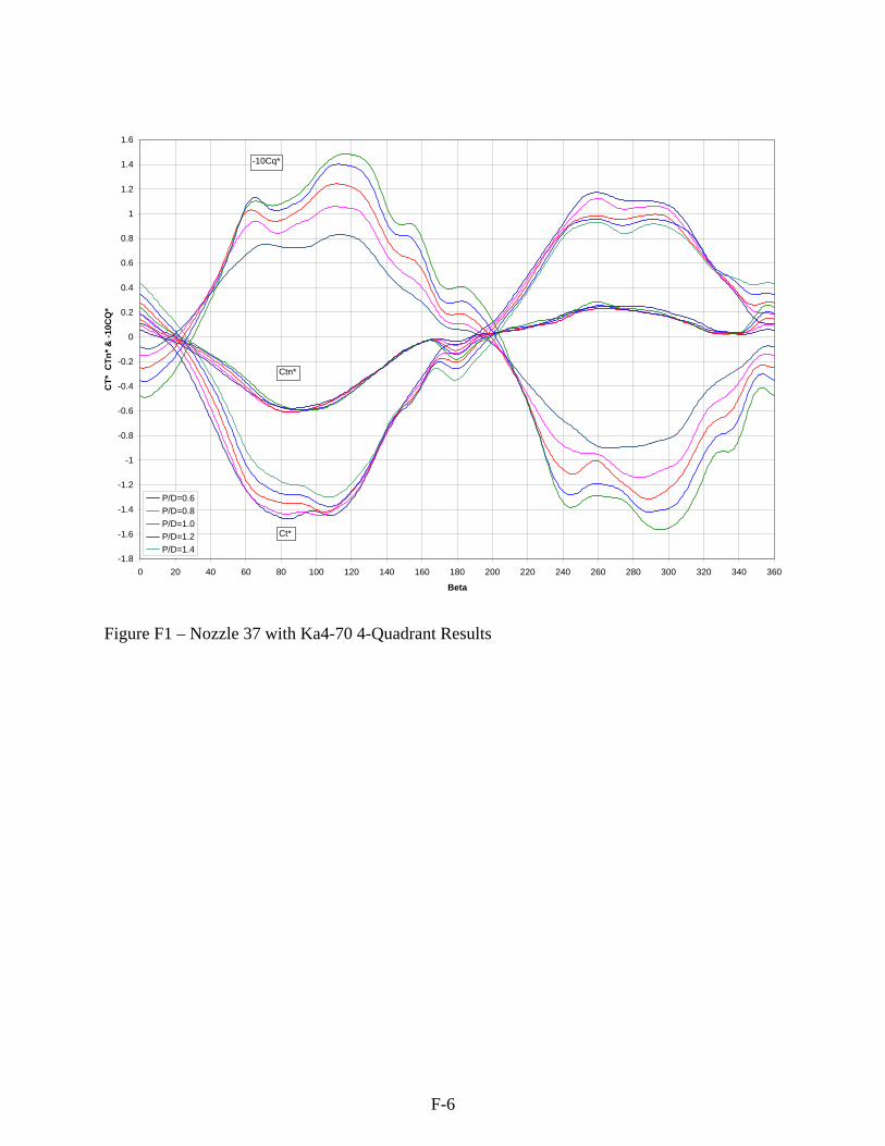
F-6

Figure F1 – Nozzle 37 with Ka4-70 4-Quadrant Results

-1.8

-1.6

-1.4

-1.2

-1

-0.8

-0.6

-0.4

-0.2

0

0.2

0.4

0.6

0.8

1

1.2

1.4

1.6

0 20 40 60 80 100 120 140 160 180 200 220 240 260 280 300 320 340 360

Beta

CT*

CTn

* & -1

0CQ

*

P/D=0.6P/D=0.8P/D=1.0P/D=1.2P/D=1.4

Ct*

Ctn*

-10Cq*

INITIAL DISTRIBUTION

Copies Organization Code Letter Only

Paper Copy

PDF Name

1 NAVSEA 05H Y M. King 2 ONR 333 Y R. Joslin, P. Purtell 1 MARIN Y Y J. Holtrop 1 Y M.W.C. Oosterveld 1 Y W. Faller 1 NSWCCD 3442 Y Y TIC(C) 1 NSWCCD 5010 Y Administrative Office

w/o enclosure 1 NSWCCD 5060 Y D. Walden 1 NSWCCD 5080 Y B. Cox 3 NSWCCD 5200 Y W. Day, G. Karafiath,

H. Liu 4 NSWCCD 5400 Y R. Szwerc, M.

Donnelley, K. Remmers, M. Wilson

3 NSWCCD 5600 Y E. Ammeen, J. Murray, T. Fu

3 NSWCCD 5600 Y Y K. Junghans, D. Hess, R. Roddy

Neural Network Predictions of the 4-Quadrant Wageningen ...

Documents

Transcript of Neural Network Predictions of the 4-Quadrant Wageningen ...