Neural Network Part 4: Recurrent Neural...

Neural Network Part 4: Recurrent Neural Networks

CS 760@UW-Madison

Goals for the lecture

you should understand the following concepts• sequential data• computational graph• recurrent neural networks (RNN) and the

advantage• training recurrent neural networks• LSTM and GRU• encoder-decoder RNNs

2

Introduction

Recurrent neural networks

• Dates back to (Rumelhart et al., 1986) • A family of neural networks for handling sequential data, which

involves variable length inputs or outputs

• Especially, for natural language processing (NLP)

Sequential data

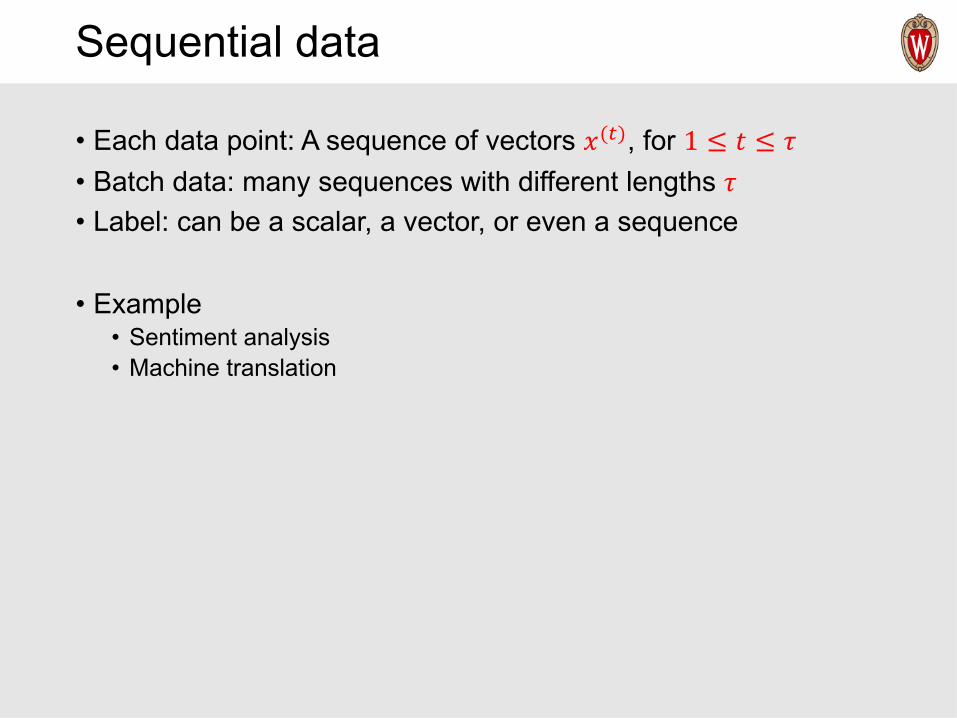
• Each data point: A sequence of vectors 𝑥(#), for 1 ≤ 𝑡 ≤ 𝜏• Batch data: many sequences with different lengths 𝜏• Label: can be a scalar, a vector, or even a sequence

• Example• Sentiment analysis• Machine translation

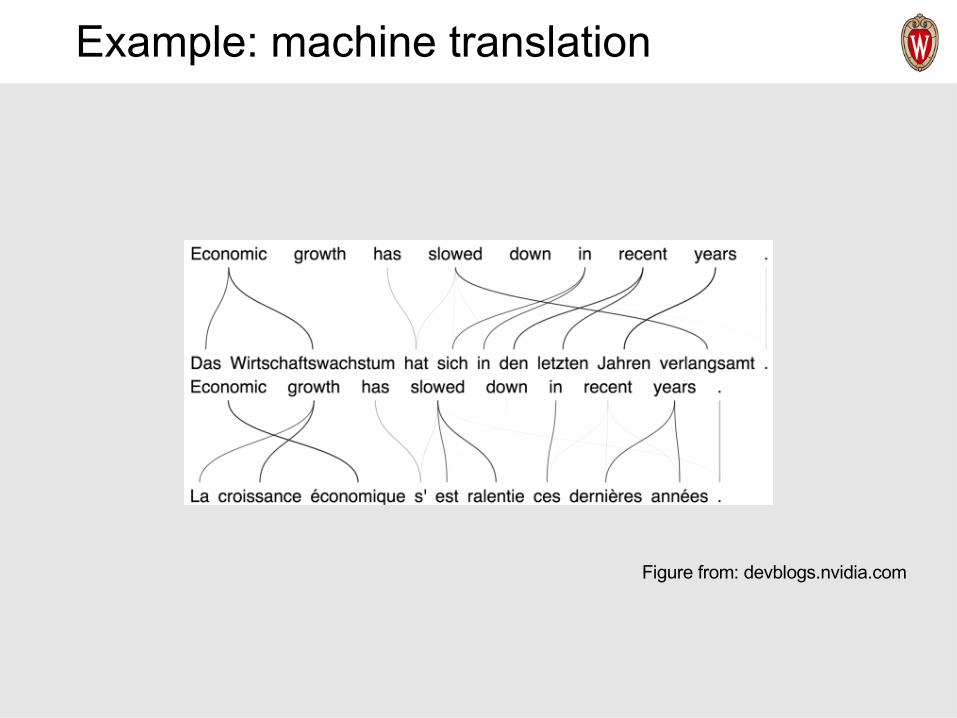
Example: machine translation

Figure from: devblogs.nvidia.com

More complicated sequential data

• Data point: two dimensional sequences like images• Label: different type of sequences like text sentences

• Example: image captioning

Image captioning

Figure from the paper “DenseCap: Fully Convolutional Localization Networks for Dense Captioning”, by Justin Johnson, Andrej Karpathy, Li Fei-Fei

Computational graphs

A typical dynamic system

𝑠(#*+) = 𝑓(𝑠 # ; 𝜃)Figure from Deep Learning, Goodfellow, Bengio and Courville

A system driven by external data

𝑠(#*+) = 𝑓(𝑠 # , 𝑥(#*+); 𝜃)

Figure from Deep Learning, Goodfellow, Bengio and Courville

Compact view

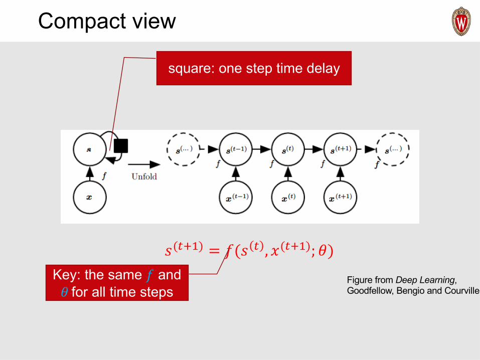
𝑠(#*+) = 𝑓(𝑠 # , 𝑥(#*+); 𝜃)


Compact view

𝑠(#*+) = 𝑓(𝑠 # , 𝑥(#*+); 𝜃)


Key: the same 𝑓 and 𝜃 for all time steps

square: one step time delay

Recurrent neural networks (RNN)


• Use the same computational function and parameters across different time steps of the sequence

• Each time step: takes the input entry and the previous hidden state to compute the output entry

• Loss: typically computed at every time step


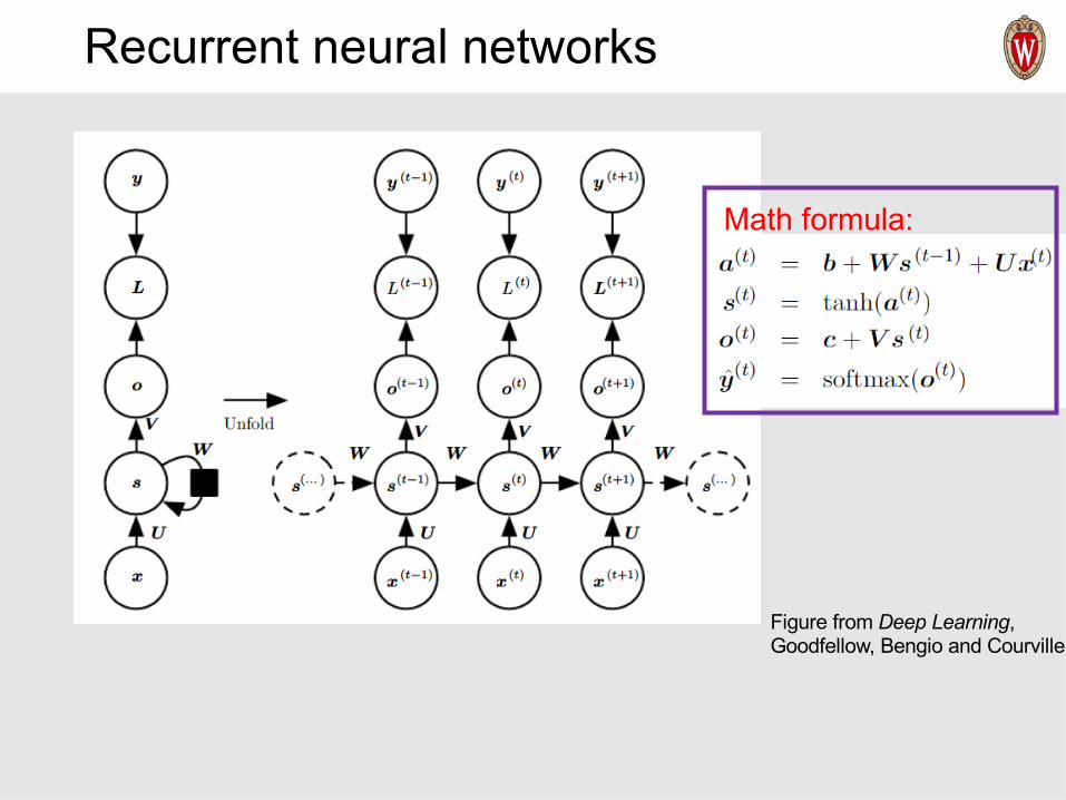
Figure from Deep Learning, by Goodfellow, Bengio and Courville

Label

Loss

Output

State

Input



Math formula:

Advantage

• Hidden state: a lossy summary of the past• Shared functions and parameters: greatly reduce the capacity

and good for generalization in learning• Explicitly use the prior knowledge that the sequential data can

be processed by in the same way at different time step (e.g., NLP)

Advantage

• Hidden state: a lossy summary of the past• Shared functions and parameters: greatly reduce the capacity

and good for generalization in learning• Explicitly use the prior knowledge that the sequential data can

be processed by in the same way at different time step (e.g., NLP)

• Yet still powerful (actually universal): any function computable by a Turing machine can be computed by such a recurrent network of a finite size (see, e.g., Siegelmann and Sontag (1995))

Training RNN

• Principle: unfold the computational graph, and use backpropagation

• Called back-propagation through time (BPTT) algorithm• Can then apply any general-purpose gradient-based techniques

Training RNN

• Principle: unfold the computational graph, and use backpropagation

• Called back-propagation through time (BPTT) algorithm• Can then apply any general-purpose gradient-based techniques

• Conceptually: first compute the gradients of the internal nodes, then compute the gradients of the parameters



Math formula:



Gradient at 𝐿(#): (total loss is sum of those at different time steps)



Gradient at 𝑜(#):



Gradient at 𝑠(3):



Gradient at 𝑠(#):



Gradient at parameter 𝑉:

• What happens to the magnitude of the gradients as we backpropagatethrough many layers?

– If the weights are small, the gradients shrink exponentially.

– If the weights are big the gradients grow exponentially.

• Typical feed-forward neural nets can cope with these exponential effects because they only have a few hidden layers.

• In an RNN trained on long sequences (e.g. 100 time steps) the gradients can easily explode or vanish.

– We can avoid this by initializing the weights very carefully.

• Even with good initial weights, its very hard to detect that the current target output depends on an input from many time-steps ago.

– So RNNs have difficulty dealing with long-range dependencies.

The problem of exploding/vanishing gradient

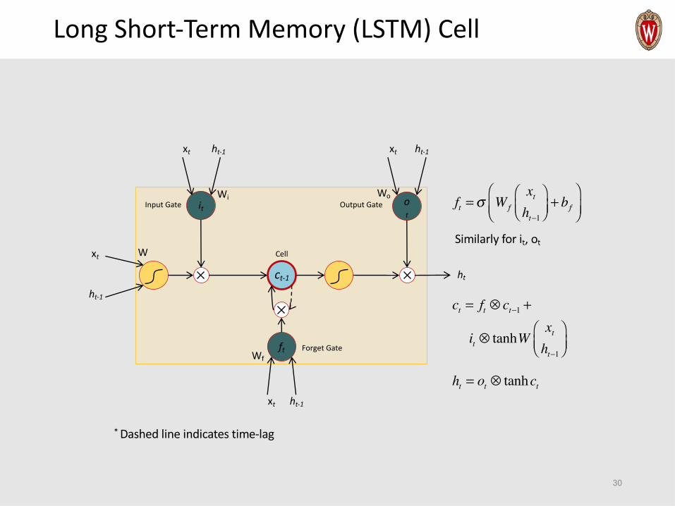
Long Short-Term Memory (LSTM) Cell

it ot

ft

Input Gate Output Gate

Forget Gate

ht

30

xt ht-1

Cell

ct-1

ct = ft ⊗ ct−1 +

it ⊗ tanhWxtht−1

⎛⎝⎜

⎞⎠⎟

xt ht-1 xt ht-1

xt

ht-1

W

Wi Wo

Wf

ft =σ Wf

xtht−1

⎛⎝⎜

⎞⎠⎟+ bf

⎛⎝⎜

⎞⎠⎟

ht = ot ⊗ tanhct

Similarly for it, ot

* Dashed line indicates time-lag

Gated Recurrent Unit (GRU) Celll

31Figure modified from Christopher Olahhttps://colah.github.io/posts/2015-08-Understanding-LSTMs/

any

Seq2seq (Encoder Decoder)

e1e0

x1

e2

x2

e3

x3

e4

x4

e5

x5

e6

x6

e7

x7

d1

y1

d0 d2

y2

d3

y3

d4

y4

知识就是力量 <end>

<end>powerisknowledge

Good for machine translation

Two RNNs

Encoding ends when reading <end>

Decoding ends when generating <end>

All input encoded in e7 (difficult)

Encoder can be CNN on image instead(image captioning)

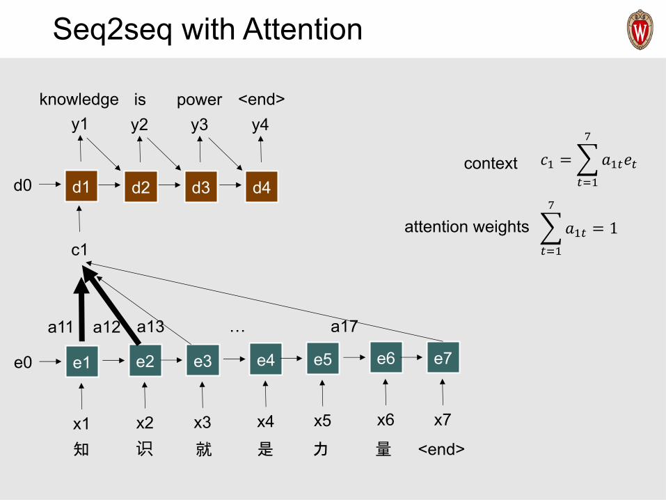
Seq2seq with Attention

e1e0

x1

e2

x2

e3

x3

e4

x4

e5

x5

e6

x6

e7

x7

d1

y1

d0 d2

y2

d3

y3

d4

y4



a11 a12 a13 a17…

c1

𝑐+ =6#7+

8

𝑎+#𝑒#

6#7+

8

𝑎+# = 1

context

attention weights

Seq2seq with Attention

e1e0

x1

e2

x2

e3

x3

e4

x4

e5

x5

e6

x6

e7

x7

d1

y1

d0 d2

y2

d3

y3

d4

y4



a21 a22 a23 a27…

c2

𝑐; =6#7+

8

𝑎;#𝑒#

6#7+

8

𝑎;# = 1

a24

… and so on

Attention weights

e1e0

x1

e2

x2

e3

x3

e4

x4

e5

x5

e6

x6

e7

x7

d1

y1

d0 d2

y2

d3

y3

d4

y4



a21 a22 a23 a27…

c2

a24

ast: the amount of attention ys should pay to et

ds-1

et

zst

as. = softmax(zs.)

https://arxiv.org/abs/1409.0473https://arxiv.org/abs/1409.3215https://arxiv.org/abs/1406.1078

THANK YOUSome of the slides in these lectures have been adapted/borrowed from materials developed by Yingyu Liang, Mark Craven, David Page, Jude Shavlik, Tom Mitchell, Nina Balcan, Matt Gormley, Elad Hazan, Tom Dietterich, Pedro Domingos, and Geoffrey

Hinton.

Neural Network Part 4: Recurrent Neural...

Documents

Transcript of Neural Network Part 4: Recurrent Neural...