Neural network on a Robot

By: Utkarsh Lath(utkarshl), Arun Kumar Rajput (akrajput)

Contents Introduction Biological Basis High Level Design Hardware Design Mechanical Design Software Design Results Conclusions Appendix A: Overall Schematic Pictures Video

Introduction Our project consists of an elementary neuron network that used Hebbian Learning to train a

robot to respond to the environment.

First, we decided to take up a task challenging enough involving electronics along with some programming and involving as many features of atmega as possible. We found this project from internet

and we found this task interesting as well as challenging enough. One of the most common examples of conditional learning such as Hebbian learning is seen in Pavlov’s experiment with his dog. In this experiment, when food was offered to the dog, it caused the dog to salivate. At first the sound of a doorbell elicited no such response. However, Pavlov decided to sound the bell when he offered food to the dog. After a few repetitions of this experiment, the dog began to salivate at the sound of the bell even when no food was present. Here food was the unconditioned stimulus, and the doorbell was the conditioned stimulus. Similarly, in our robot when we first shine light on the robot from different directions it has no effect on the robot. We then press the button while shining the light from a particular direction on the robot and the neural network programmed into the robot causes it to associate the light input with the push button input according to how it was trained initially. Say, every time I give light from forward direction, I press left button. Soon the robot learns to move in the left direction when light is shined from the forward direction. There are other neurons in this network that play an inhibitory role and prevent the robot from going too close to the light.

Biological Basis

Back to top

A neuron consists of a cell body with dendrites and an axon which terminates onto a muscle fiber or the synapse of another neuron. It receives signals in the form of charges (sodium, potassium, calcium ions) from other neurons that have their axons terminals sharing synapses with its dendrites. These charges are integrated spatially (across number of neurons that synapse onto it) and temporally (charges received over time) and change the membrane potential of the neuron. The membrane potential usually increases with the influx of sodium ions and the efflux of potassium and calcium ions. An increase in membrane potential is also referred to as a depolarization. Once the membrane potential increases beyond a certain threshold potential, specific for the particular neuron, an action potential is fired. Action potentials are characterized by a strong depolarization, followed by a hyper polarization (decrease in membrane potential). The action potential is then transmitted down the axon to the axon terminals where it is passed onto the next neuron through a synapse.

Action potentials are ‘all or none events’ and their method of generation can be characterized by an ‘integrate and fire’ approach. That is, a cell integrates charge signals it receives from other neurons and only after its threshold is reached it fires an action potential, thereby transmitting a signal to its postsynaptic neuron. After firing this action potential, the firing neuron goes through a refractory period. During this time, it cannot fire another action potential even if the signals it receives push its membrane potential beyond its threshold value. At the end of the refractory period the membrane potential is at its resting state. All of the charge entering a neuron from other cells does not contribute to the rise in membrane potential. Some of the charge is constantly leaking out of the neuron. This is called leakage current.

Neurons connected in a network can be used to display Hebbian Learning. Donald O. Hebb a Canadian Neurophysiologist proposed the following postulate:

When an axon of cell A is near enough to excite a cell B and repeatedly or persistently takes part in firing it, some growth process or metabolic change takes place in one or both cells such that A's efficiency, as one of the cells firing B, is increased.

http://neuron-ai.tuke.sk/NCS/VOL1/P3_html/node14.html

The principles underlying his postulate came to be known as Hebbian Learning. Therefore, if two neurons in a network (a post-synaptic and pre-synaptic) neuron fire repeatedly in the correct order, the connection between them is strengthened. The order in which neurons fire is very important. If a presynaptic neuron fires shortly before the post-synaptic neuron their connection is strengthened, however if the post-synaptic neuron fires shortly before a presynaptic neuron then the connection is not affected. If the time interval between the firings of these two neurons is very large, they cannot be correlated. The following diagram shows how the timing of action potential (also referred to as spikes) affect the weights between a two neurons.

Figure 1 Biological Model for Change in Weights

Back to Top

High Level Design • Rationale•

Background Math:

• Logical Structure: • Standards:

time

change in weight

Rationale: At first, we had a hard time choosing a final project idea. We got the idea of this project from

internet. Some students had done a similar project but on 1 dimension and some fewer features(link). After doing research on the idea, we found it very interesting because not only the topic was new and very interesting but also very informative about how we actually learn. Building a neural network on a robot would make it appear quite realistic and funny like some real world phenomena. So we decided to build a robot that would use a neural network to learn to react to certain stimuli. At first we thought of using IR light as an input into the system, but after some thorough discussion, we realized that doing that would cause a lot of troubles. Finally, we settled on using a light-guided robot as the real world interface for the project. Light turned out to be a convenient input because LDRs were cheap and quite reliable to be used as analog light sensors and then we came up with an ingenious arrangement to get rid of environment light and only detect light from torch. This served our needs perfectly. Their directionality was also good enough from torches to guide our robot. Our inspiration for using light came from how a moth is always attracted to light, but when it gets too close to a light, it will quickly fly away due to in the intense heat. The attraction to the light shows excitation while the aversion at close proximity shows an inhibitory effect. We decided to model this type of system where there would be multiple layers of Hebbian learning.

Background Math: Integrate and Fire Equations:

Temporal & Spatial Integration of voltage:

τdV / dt = V rest + V exc + Vinh

Where τ is our decay constant. Vrest is the resting membrane potential which we set to 0; Vexc is the voltage inputs due to excitatory connection and Vinh is the voltage inputs due to inhibitory connections.

The weights were updated according to the following equation:

Wij = Wij + Tij

Where i corresponds to the presynaptic neuron, j corresponds to the postsynaptic neuron and Wij is weight of the connection; Tij is the weight of the connection * Learning rate.

Logical Structure: We did the design process in many logical stages. The first stage was to get the hardware

working. We soldered the PCBs and planned our IO pins and other things. We took some time (10 days) to get the motors working via motor driver. We first designed simple programmes for remote control, LDR usage, timers, LCD etc. We then made a 2 dimensional neural network without inhibition and the outputs and weight were displayed simply on the LCD and got the network working by seeing the weighs change. After getting the motor control working, we integrated this with the neural network programme to make sure that the network was working fine and showing the learning characteristics which we managed to achieve after few corrections. Finally, we added time decaying unlearning, inhibition

features and a special function to show the arbitrariness of the simplified output function and how powerful this learning technique is. Then, we would shine light from any of 4 directions and show that the robot moves and there exists both excitatory and inhibitory effects. There will also be real-time learning and unlearning as the robot is moving through its light course.

The following is an overview block diagram of the overall project.

Figure 2: Overall Flow of Project

The neural network has 9 inputs (4 light sensors and 5 pushbuttons four for motion in 4 drn and one for special function) and 5 outputs (moving in one or more of the 4 directions or the special function). The following diagram shows the network, where solid lines indicate excitatory connections and dashed lines indicating inhibitory connections.

Input (environment, i.e. lights) pushbuttons)

Neural network code programmed on atmega

Output (LCD) the change of weights and excitation of neurons

Motor driver Motor movement (Robot moves)

Forward motor

Forward push button

Backward motor

Right motor

Left motor

Special function

Backward push button

Right push button

Left push button

Special function

Forward light

Backward light

Right light

Left light

LDR input Output neuron

Push button input neuron

Inhibitory neuron Excitatory neuron

Constant weight connections Figure 3: Schematic of the Neural Network

Explanation:

Motion Pushbutton: The input to this neuron is the push button press. It has an excitatory connection to the forward motor neuron with a very large constant weight since it represents the ‘unconditioned stimulus’ to the network, we do not want our network to behave unruly or become involuntary.

LDR:

(I) Excitatory: This takes in as input the voltage from the light sensor. This has an excitatory connection to all the motion output neurons. It will get excited only if the light is not too strong.

(II) Inhibitory: This also takes in the voltage from the light sensor as an input. The difference between this and the excitatory neuron is that this has a much higher threshold. Thus, if the input voltage from the front sensor is high, it means that the robot is pretty far from the front light source and is in no danger of being burned. But, if the robot is very close to a front neuron, then this neuron will spike very frequently. This is to warn the robot that it is too close and should not proceed as quickly in the front direction. Thus, if this neuron fires, it actually inhibits the corresponding motion output neuron. Furthermore, if this neuron fires, it is also telling the robot that it should move in the opposite direction to be safer, so it has an excitatory non constant connection to the opposite motion neuron.

Output Neuron:

The Output neurons are responsible for driving the motor whenever they excite. Outputs of all the neurons are superimposed on each and a special function ‘movefr’ is called which conveys the final output to the motor driver.

Standards: There really are no standards we needed to worry about in this project. Our goal was just to build a biologically correct network that simulated learning, so the main “standard” we used was the process of Hebbian learning.

More information on the process of coding the actual neurons is in the programming details section.

Hardware Design Back to Top

The most fundamental part of our system was the hardware part. We had to design the robot and motor controls. The robot is controlled by two simple 200 rpm 12 V motors, and each moves backwards or forwards depending on which neuron fires. We also decided to build a stand-alone Mega16 prototype unit which would just be on the robot. Furthermore, a very important part of the project was to demonstrate the learning process of the robot through the neural network. To do this, we need to use LCD to real-time output the continuously changing weights of the network. Thus, during the initial learning phases, LCD is essential to demonstrate that the neural network is indeed working

properly. All this, we had to do on soldered boards for all our parts. These boards are lighter, neater and more portable for the final product and also take up less space.

• LCD • LDR • Remote • Motor Stuff • Power Sources

LCD: To use LCD all we had to do was to make hardware connections to the PORTC of the mcu as required and the power connections. Once done we had to use functions from lcd.h file to get going.

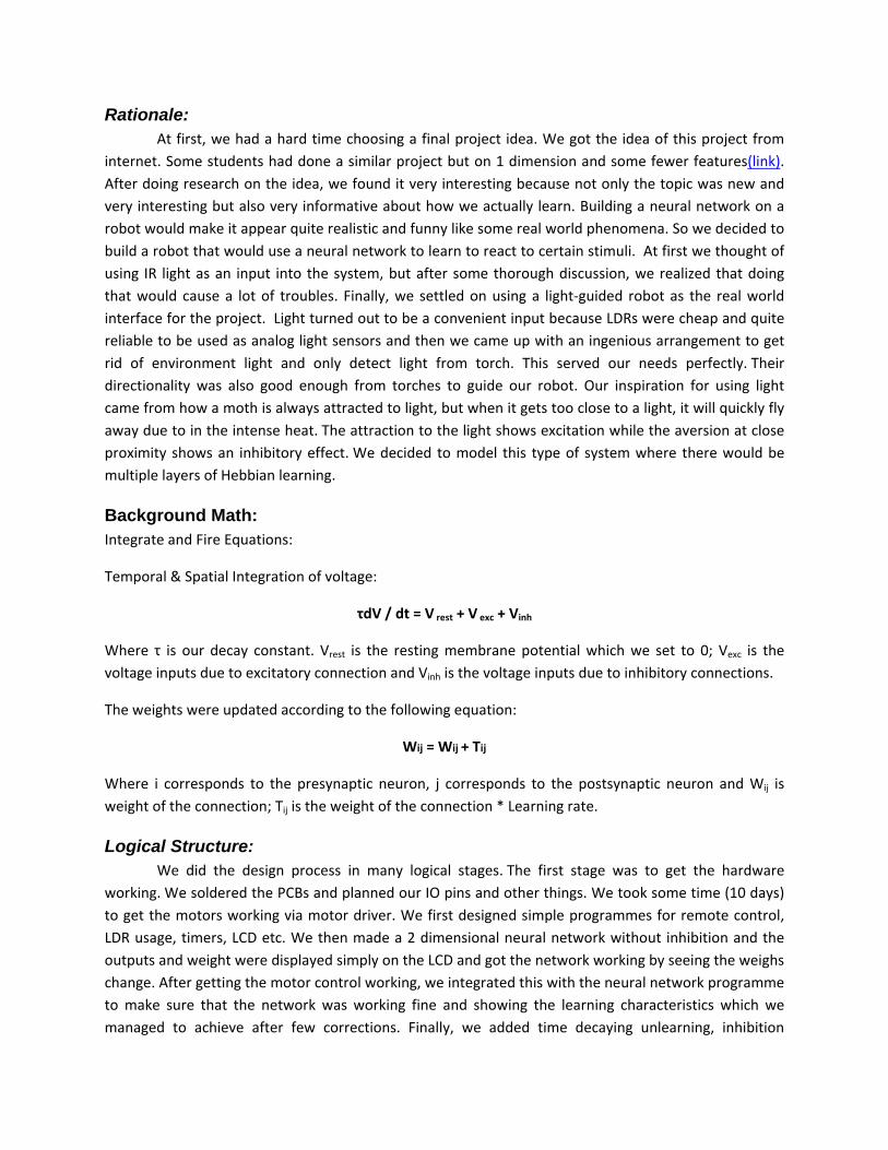
LDR: LDR were used as analog light sensors in series with a 300 OHM resistor. These LDRs are cheap, directional, sensitive, and easy to use, making them great parts as analog light sensors. The LDR voltage output went into PORTA of the MCU, which is the ADC. The following is a diagram of the light sensing circuit.

Figure 5: Hardware for LDR input in ADC

For very strong Light the ADC reading was below 50 for medium light the output was below 150 and when no torch light falls it was above 200. The output of the 4 LDRs were slightly different when exposed to strong light so we made some correction in the values. The code for using the LDRs is given here.

LDR Code

Remote: As we had only 10 pin connectors available, to keep everything simple, we could only have 8 different controls on our remote and 2 wires were used as +5 V and ground. Our controls were 4 direction

controls, one potentiometer for speed and 3 toggle buttons for instantaneous stop, stop learn/unlearn and reinitialize. However, later we used the third one for special function.

Motor Stuff: We used two 200 rpm 12 V DC motors for our project. This motor rotates depending on the

direction in which current flows. When flows from terminal, say A to terminal B it is, say clockwise and when B to A, it mover counter-clockwise. The speed of the motor is controlled by varying PWM, i.e. rapidly switching motor on and off for different time periods, say on for 3 ms and off for 1 ms. However these motors draw large amt of current of the order of 500 mA and also need 12 V operational voltage therefore we need a motor driver to serve this purpose.

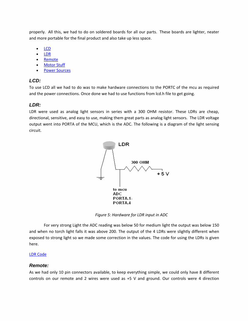
To drive the motors, we used a L293, since the motors cannot be run directly from mcu because it operates on 12 V and also mcu cannot handle so much current. This device, provides enough current and power to control the motor. We only needed to use one L293 to control both the motors. We used PORTB from the MCU as the output port to control the motor. The output from Atmega goes into the input of the L293. The outputs of the L293 are wired directly into the motors. The following is a schematic of how to use the L293 to drive the motors. Two output pins of the atmega are devoted for each motor and 1 for common PWM. To drive of the motors all you need to do is provide (0, 1) or (1, 0) on the two pins. We give (0, 0) when we do not want it to move and (1, 1) to immediately stop the motor.

Figure 4: Schematic of L293 Motor Driver

Once the motor connections were made, we had to add in the motor code. Before integrating the motors, we used test code to help us debug our wiring and determine the best ways to wire it. The following was the test code with remote control that we used:

Motor code

Power source: DC +12 V Adapters were used as power sources and 7805 was used to power the mcu. The motor driver and the mcu were given power via different and independent sources because of some current rating problems between the adapters and the motors.

Mechanical Design

Back to top

Another aspect was the mechanical design of the project. The base of the robot is a piece of wooden board. We used brackets to secure the motors. Each of the two motors was attached to a wheel, and we used a castor wheel in front because it is fairly frictionless and thus easy to move.

There was also a problem of mounting the LDRs in the 4 directions permanently. So we fixed an L shaped arrangement to the back end of the robot and fixed our LDR network onto it.

Software Design

Back to Top

Full Programme

We programmed the network in various stages and tested each part before integration. Each input neuron on the network had the following variables associated with it:

Input Neuron:

V: Represents the current voltage of the input neuron.

Time: used to countdown time whenever the neuron excites.

Threshold: variable denoting the threshold potential for the neuron.

Excite: used to indicate weather the neuron has excited in this cycle.

Output Neuron:

Voltage: same as V above.

Time: same as above.

Threshold: same as above.

Excite: same as above.

Efficiency[]: Stores the efficiencies of all the input neurons at this output neuron.

Connection time[]: Stores time for the purpose of time decay of the corresponding weight.

Concept involved:

Stage 1:

Structure of Network: This network consisted of twelve neurons, 4 pushbutton neuron s, 4 light neurons and 4 motor neurons. Each type of neuron was coded separately because their membrane potentials were updated differently and thus could not be effectively generalized in a loop. In the case of the push button neuron, when a button was pushed, it added its threshold to its membrane potential. The light input neuron added the input from the respective sensor of the ADC on the MCU chip. The motor neuron updated its membrane potential by adding the weights of its presynaptic neurons that had fired in the present cycle to its current membrane potential. After the membrane potentials were updated in a specific neuron of the network, the code checked to see if the membrane potential was greater than the threshold voltage for that neuron. If it was, the excite variable for that neuron was set to 1, indicating a spike, and time was set to refractory, which indicated that the neuron had entered a refractory period of length refractory (in ms).

Change of weights: In this section what had to be done was to see if an output neuron has neuron has recently fired. If so check if any of the light sensors has peaked and if so increase the corresponding weight. Also the weights were caped that is if some weight went above 1 or below the minimum allowed limit, it was set back to the border value. The model that was used to update the weights is an approximation of the biological model shown below. Increase in weight is by a factor which determines how quickly the robot learns, called LRATE.

dT

Change in weights Increase in weight

No change

Figure 6: model of weight change graph.

Time decay of weights: The concept is that every non constant connection is monitored and all those connections that show no change for a threshold time (DecayTime) are decremented by a certain factor (Decayrate) which determines together with the DecayTime, the unlearning rate.

Output section: This was the most important section as this was very important in the beginning when we had to do debugging. We decided to follow the following scheme to best utilize our 16*2 LCD display:

In the scheme, the voltages are shown on a linear scale (‘A’ to ‘Z’, ‘A’ for 0 voltage ‘Z’ for voltage close to 1) as long the neurons are not excited. Once the neurons go excited, instead of ‘A’-‘Z’ 1-3 are written to show which neuron has excited. Direction of motion indicator shows ‘L’/’R’ for left/right rotation and ‘F’/’B’ for forward/backward motion. PWM is also on a linear scale (‘A’ to ‘Z’, ‘A’ for 0, ‘Z’ for voltage close to 255).

The weight display scale is logarithmic scale because learning/decaying is also exponential change on the value of weights. The initial value is chosen ‘A’ and anything above ‘A’ in the display indicates that it has learnt more than unlearnt and the changing of weights indicates learning/decaying.

Stage 2:

Structure of Network: In this stage we decided to add inhibitory neuron to the network. This neuron also received its input from the same ADC pin but its threshold is set much higher. All other variables are similar to input neuron except for wtOppDrn which is the weight of the connection between this inhibitory neuron and the opposite direction motion neuron. The role of this neuron is to stop the motor from going too close to the light even if accidentally the corresponding motion button is pressed. It achieves its purpose by reducing the membrane potential of the motor neuron to which it is connected. Also it induces the robot to move in opposite direction because it has excitatory connection with the motor neuron of opposite direction.

Change of weights: The weight adjustment for this additional neuron is similar to the weight adjustments described in the previous stage. The weight of the inhibitory neuron is fixed in the direction of neuron, and the excitatory connection in the opposite direction is increased if the corresponding output neuron activates.

Output section: No changes were made in this section since the inhibitory action worked nice at first run so we didn’t had to do much debugging and hence output section was kept as it was.

Stage 3:

Structure of Network: We decided to add another input and output neuron to the system, the input neuron would peak if the robot detects an obstacle in front and the output function would just be special hardcoded function basically to avoid the obstacle but it could be anything. We decided to use TSOP sensor to detect obstacle, however somehow we could not manage to get the electronics of TSOP working, so we left this part but it we did not delete the coding we had done. We still implemented the special function feature, so finally our network appeared as shown in Fig 3. The new output neuron was connected to all the input neurons and assigned a toggle button on remote for this task. The special function we hardcoded took 1.5 sec to execute so the learning rate for connections to this neuron were kept very high so that it would learn in 3-4 cycles only to make it better presentable This special function could be coded differently and come very useful when we start thinking about further extensions of this project like it would be the task to pick up the obstacle once we attach tentacles to the robot. Everything else is very similar.

Change of weights: The weights for the extra added output were just same as earlier other than the fact that all connection to the new neuron had very high learning rate.

Timing Section:

Neural network time: All the neurons in the network and their weights were updated every 10 ms which means that τ was set to 10 ms. the refractory period was set to 50 ms. The refractory period had to be at least twice as long as it takes to update every neuron in the network. The reason for this can be seen from the model that was used to change weights of the neuron.

Figure 10: Timing of Neural Network

Global Constants

LRATE (0.15): The Rate at which the robot learns.

Number of cycles taken to fully learn=log ( 1/ initial efficiency)/log(1+LRATE) is to be kept optimum.

LRATEtSOP (3): The number of cycles is to be kept around 3-4 in this case.

Decaytime(500),Decayrate(0.2): This parameter along with the decay rate decides how rapidly the weights should decay. These values seem to optimize the rate of unlearning.

DecayrateTSOP(0.05): The decay rate for the special function. Has to be kept rather low.

Leakage(0.9): The rate at which the current leaks. Has to be kept so that without training the light cannot excite motion in any direction, i.e. solving

X= (Leakage)*(x+4*EfficiencyInit), x should fall much below threshold, because it is the equilibrium value of the voltage.

refractory(50): The refractory period for which the neuron remains inactive once excited. Close to the biological value.

DELAY(10): The period after which the voltage is integrated ( τ ).

EfficiencyInit(0.005): The initial weight between excitatory neurons.

EfficiencyInitTSOP(0.01): The initial weight of the connections to the special function neuron.

MinEfficiency(0.001): The lowest efficiency allowed.

Back to Top

Results • Accuracy • Safety and Interference • Usability

In the end, all three portions of the project accomplished the goals we set out to in the beginning. The mechanical design produced a robot that would move appropriately whenever the motor neurons spike. Good hardware arrangements were made so that LDRs detected light only from the torch and from no where else. The wiring for the motors worked well because we were able to get enough torque and pulse the robot correctly. The crux of our project, the neural network, worked as we hoped it would too. Since the algo of neural is only an approximation of the exact behavior we expected some randomness but to our surprise the behavior in every trail was very deterministic and just as it was expected to behave. We had to settle down with the exact values of the parameters so that our robot was best usable and that made its learning action appear very clearly. We settled with a rather slow learning rate for excitatory neurons and slow unlearning rate for inhibitory neurons and very fast learning rate for special function so that all the features were clearly visible at the surface. We also used LCD to examine and to ensure the learning as well as of decay of weights.

Outside factors such as the type of light source and the amount of ambient light adds some amount of ambiguity in our project in the sense that LDR can only sense intensity so we had to calibrate our programme according to the light source that when it should consider the light is strong enough to inhibit and when it should just excite. Therefore out robot would behave differently to different light sources though we never tried this out. To deal with this, we would have to measure the voltage output of the LED whenever we used a different light.

Our coding was split into various stages: simple network with only excitatory connections, then we added inhibition and at last the special function feature to the robot.

By splitting the neural network into stages, we were able to add complexity as the project went along. Thus, we were able to prefect smaller networks first, and then only after this worked, did we build extra features such as inhibition and special functions into it. Our goal in the beginning was just to get our excitatory network working, and by the end we were able to accomplish this goal along with some extra added interesting functionality. We were able to meet the specifications we set out to do.

Accuracy: Complete accuracy is hard to determine for the neural network because it is only a good

approximation of what should ideally happen. Overall though, we had a sense of what should happen over time. At first, the robot should only move when a pushbutton is pushed. After the robot is trained, it should be able to move only with light. If a light source is far away and the robot is trained to move toward light, the robot will slowly move towards it and as it gets closer, the excitatory neurons will fire more causing the robot to move faster. As the robot gets even closer though, the inhibitory networks will kick in stronger and the robot should start moving slower again. When the light is really close, the

robot should stop moving and actually start slowly moving in the other direction. Thus there comes to a point where the robot will just move back and forth (jittering) but won’t approach the light any more.

The speed of learning was not a problem and it could be controlled by varying the learning rate. On one hand we designed the special function to do learn over 3-4 cycles whereas the normal excitatory neurons took around 40 cycles to learn and also the decay rate of inhibitory neuron connection to opposite direction motion was pretty slow. While animals can learn, they can also unlearn so happens in our robot but we decided on having a time decaying unlearning model. Also since the algorithm is completely deterministic, the behavior was very predictable and all the trails gave almost very similar results with little variations or noise.

Safety and Interference: This project did not have many safety concerns. The main human contact involves pressing the

pushbuttons, but no part of the project is attached to the user. Thus, there was minimal safety issues involved. Also, we had no interference problems because we did not have any wireless portions in the project.

Usability: Our final product is easy to use, but the theory behind it is somewhat complicated. In order to

understand what the project is supposed to do, we have to explain how we set up the neural network and what it is supposed to do. We could also show how it should model the real world situation of a moth flying near a light. Once this explanation is done, any user could easily experiment with the project to see exactly how the neural network evolves over time and how learning actually occurs.

Back to Top

Conclusions In conclusion, our final project met all the specs that we initially set out to do. Initially, our goal

was to design a neural network that would model some real world phenomena using microcontroller and to learn the usage of microcontrollers and some real word electronics. We decided to use light and model a moth’s behavior via using a robot whose movement was controlled by the outputs of a neural network. We also wanted to build a robot with motor control to show the output and to also take advantage of the portability of the microcontroller. After we accomplished the simple learning features we realized that we could easily extend it to include more features like inhibition and add other output neuron for some special function that would make it appear fancier. Therefore, we were able to meet all our goals by building a neural network with many different Hebbian learning pathways. Furthermore, we were also able to gain sufficient experience working with electronics of the motors, sensors, mcu, power sources etc. We had sufficient experience working with mcu using its various features such as IO, timer interrupts, PWM, ADC, LCD, pull up etc.

While we are happy with out results, there are some things that could be improved. We could have added many extra features to out robot such as avoiding an obstacle or carrying some thing. Then building a neural network on those would have made it appear highly fancy. The robot would seem to

learn to avoid an obstacle and to go some other way round. Also it would appear nice if the robot could be trained to transport things from one place to other and then we would simply have to give light and the robot would learn that it has to transport the things from on place to other. It would do it automatically without any human intervention. This could be a good next step, but we thought that for our limited time duration, this much was complicated enough. We also could have put a separate battery on the robot to power the motors instead of using the power supply so that the robot would be completely autonomous and wouldn’t need wires connected to an outside power supply.

We didn’t really have any legal or intellectual property considerations to worry about in this project. While we didn’t have any standards we had to follow, we did try to model biology as closely as we could.

Back to Top

Appendix A: Overall Schematic The following is an overview of the connections to the MCU:

Back to Top

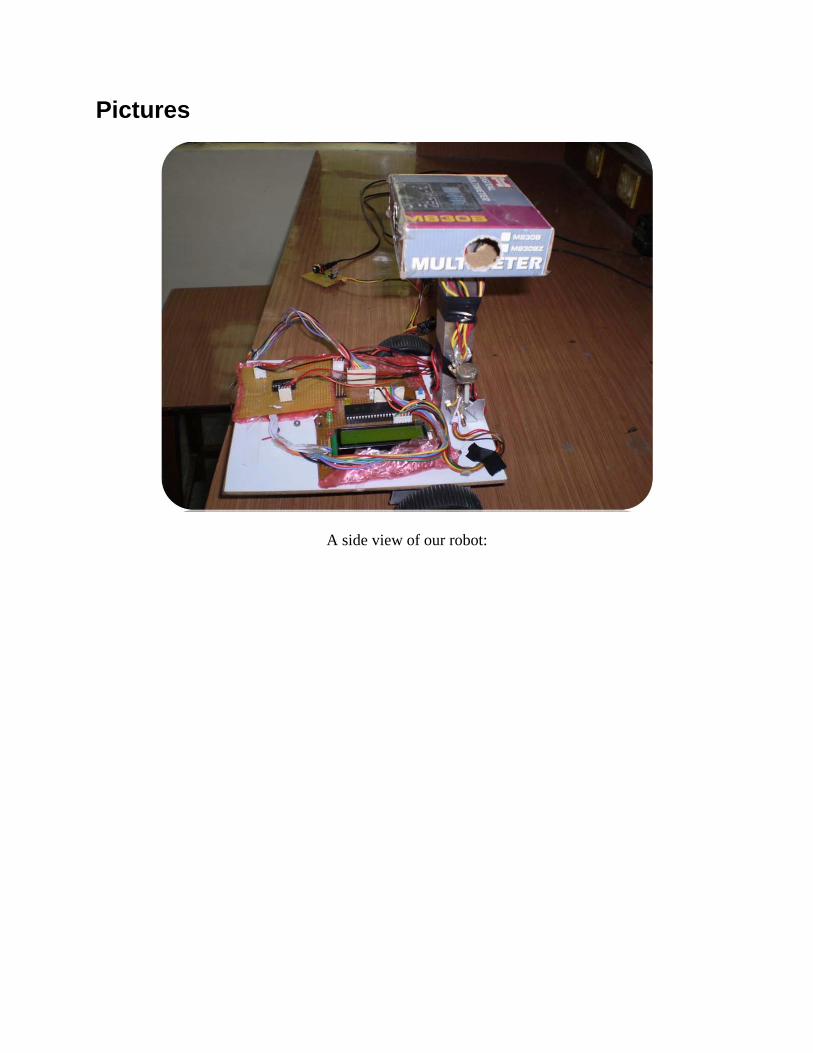
Pictures

A side view of our robot:

A Front view of our robot

Robot with its creators:

More pictures can be seen at Google

Back to top