NEURAL NETWORK MODELING OF THE DYNAMICS OF …
50
NEURAL NETWORK MODELING OF THE DYNAMICS OF AUTONOMOUS UNDERWATER VEHICLES FOR KALMAN FILTERING AND IMPROVED LOCALIZATION BY SHARAN BALASUBRAMANIAN THESIS Submitted in partial fulfillment of the requirements for the degree of Master of Science in Industrial Engineering in the Graduate College of the University of Illinois at Urbana-Champaign, 2020 Urbana, Illinois Adviser: Clinical Associate Professor William Robert Norris
Transcript of NEURAL NETWORK MODELING OF THE DYNAMICS OF …

NEURAL NETWORK MODELING OF THE DYNAMICS OF AUTONOMOUS
UNDERWATER VEHICLES FOR KALMAN FILTERING AND IMPROVED
LOCALIZATION
BY
SHARAN BALASUBRAMANIAN
THESIS
Submitted in partial fulfillment of the requirements
for the degree of Master of Science in Industrial Engineering
in the Graduate College of the
University of Illinois at Urbana-Champaign, 2020
Urbana, Illinois
Adviser:
Clinical Associate Professor William Robert Norris
ii
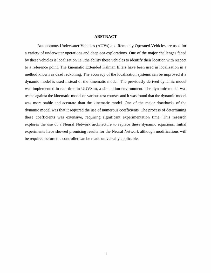
ABSTRACT
Autonomous Underwater Vehicles (AUVs) and Remotely Operated Vehicles are used for
a variety of underwater operations and deep-sea explorations. One of the major challenges faced
by these vehicles is localization i.e., the ability these vehicles to identify their location with respect
to a reference point. The kinematic Extended Kalman filters have been used in localization in a
method known as dead reckoning. The accuracy of the localization systems can be improved if a
dynamic model is used instead of the kinematic model. The previously derived dynamic model
was implemented in real time in UUVSim, a simulation environment. The dynamic model was
tested against the kinematic model on various test courses and it was found that the dynamic model
was more stable and accurate than the kinematic model. One of the major drawbacks of the
dynamic model was that it required the use of numerous coefficients. The process of determining
these coefficients was extensive, requiring significant experimentation time. This research
explores the use of a Neural Network architecture to replace these dynamic equations. Initial
experiments have showed promising results for the Neural Network although modifications will
be required before the controller can be made universally applicable.
iii
ACKNOWLEDGEMENT
I would like to express my gratitude to Dr. William Robert (Bob) Norris for his invaluable
support during my degree. His guidance helped me to grow both professionally and personally in
the last two years. I would like to thank Dr. Michael Dyer from the department of Finance for
taking me in as his Teaching Assistant and providing me with an opportunity to teach for the last
two semesters. I would also like to thank Dr. Richard Sowers and Dr. Ramavarapu RS Sreenivas
from the department of Industrial and Systems Engineering for their advice.
I would like to thank my parents for providing the necessary moral and financial support
for pursuing a Master of Science degree. I would also like to thank my roommate and my friend
Mr. Gnanendra Reddy for putting up with me and taking care of me during tough times.
My thesis research would not be possible without the contribution of my project group,
nicknamed the “Submarine Bois”. Rodra Wikan Hascaryo, one of the predecessors of this research
played a huge role by my side to help me understand and design the dynamic model. The support
provided by Sandeep Srikonda and Ayush Rajput during the implementation phase of the Kalman
Filter cannot be overstated. Two hard working undergraduate students, Chirag Rastogi and Justin
Yurkanin played a vital role in the data collection phase.
Finally, I would like to acknowledge the members of the Autonomous and Unmanned
Vehicle Systems Laboratory and my friends for their help and motivation during the last two years.
This research has been funded through a generous gift grant from Schilling Robotics, a
subsidiary of Technip FMC.
iv
TABLE OF CONTENTS
CHAPTER 1: INTRODUCTION …………………………………………………………………1
1.1 BACKGROUND ................................................................................................................... 1
1.2 METHODOLOGY ............................................................................................................... 3
1.3 THESIS ORGANIZATION ……………………………………………………………… . 3
CHAPTER 2: DYNAMIC MODEL DERIVATION FOR RexROV ............................................. 5
2.1 COORDINATE SYSTEMS AND CONVENTIONS ........................................................... 5
2.2 COMPONENTS OF THE DYNAMIC MODEL .................................................................. 6
2.2.1 KINETIC FORCES ........................................................................................................ 7
2.2.2 HYDRODYNAMIC FORCES ....................................................................................... 9
2.2.3 HYDROSTATIC FORCES .......................................................................................... 10
2.2.4 THRUSTER FORCES ................................................................................................. 10
2.3 DYNAMIC MODEL DERIVATION ................................................................................. 11
2.4 REDUCED DYNAMIC MODEL FOR RexROV .............................................................. 12
2.5 IMU ACCELERATION TEST ........................................................................................... 15
CHAPTER 3: COMPARISION OF DYNAMIC AND KINEMATIC KALMAN FILTER ....... 18
3.1 KALMAN FILTERS........................................................................................................... 18
3.2 EXTENDED KALMAN FILTER FOR RexROV .............................................................. 21
3.3 PURE PURSUIT CONTROLLER...................................................................................... 23
3.4 TEST COURSES ................................................................................................................ 25
3.4.1 BEHAVIOR EVALUATION 1.................................................................................... 25
3.4.2 BEHAVIOR EVALUATION 2.................................................................................... 26
3.4.3 BEHAVIOR EVALUATION 3.................................................................................... 27
CHAPTER 4: NEURAL NETWORK DYNAMIC MODEL ....................................................... 29
4.1 MULTI-LAYER NEURAL NETWORKS ......................................................................... 29
v
4.2 ACTIVATION FUNCTIONS ............................................................................................. 30
4.3 GRADIENT DESCENT ..................................................................................................... 32
4.4 BACK PROPAGATION..................................................................................................... 32
4.5 NEURAL NETWORK DYNAMIC MODEL .................................................................... 33
4.6 RESULTS ON THE TEST DATASET .............................................................................. 34
4.7 ARCHITECTURE SELECTION ........................................................................................ 36
4.8 NEURAL NETWORK MODEL VS DYNAMIC MODEL ............................................... 37
4.8.1 BEHAVIOR EVALUATION 1.................................................................................... 37
4.8.2 BEHAVIOR EVALUATION 2.................................................................................... 38
4.8.3 BEHAVIOR EVALUATION 3.................................................................................... 39
CONCLUSION ............................................................................................................................. 41
REFERENCES ............................................................................................................................. 43
1
CHAPTER 1: INTRODUCTION
1.1 BACKGROUND
The planet Earth consists of 71% water and 29% land. Recent scientific advancements have
enabled us to put satellites on space to monitor various events on Earth. These geo-spatial satellites
can provide us information about the surface temperature of oceans, the direction of ocean currents,
color of ocean bodies etc. But what these satellites lack is their ability to look deeper into the
oceans in 3D. According to Gene Feldman, we have more knowledge about the surface of Mars
than that of our ocean bodies [1]. At deeper depths, the pressure exerted by these cold and dark
waters is enormous. Luckily, we have Autonomous Underwater Vehicles (AUVs) and Remotely
Operated Vehicles (ROVs) for underwater and deep-sea explorations.
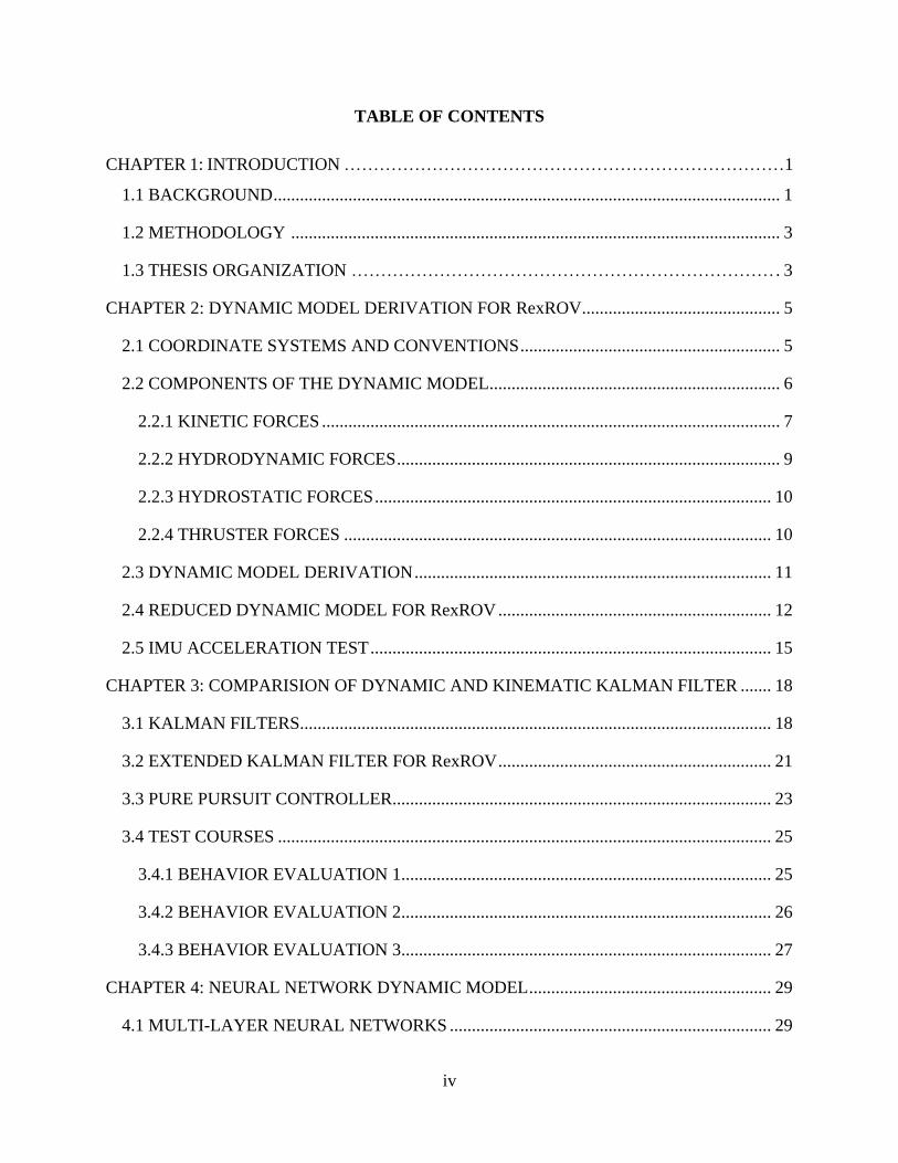
The most basic type of ROV is the RexROV and it is based on the SF 30k ROV [2]. It has
four lateral thrusters and four vertical thrusters for maneuvering purposes. The four lateral thrusters
are responsible for its movement along the x and y axis. The four vertical thrusters ensure that the
vehicle remains floating when it is stationary and are responsible for movement along the z-axis.
The RexROV with the thrusters is shown below.
Figure 1: RexROV with thrusters
Experimentation with an AUV was difficult since it was hard to control the nature of the
environment in which they were operated. A realistic simulation will greatly help in reducing the
risks and costs involved in validating several aspects of a project. There are two major simulator
environments used in reference to underwater robotics. One is UWSim [2] and the other is
2
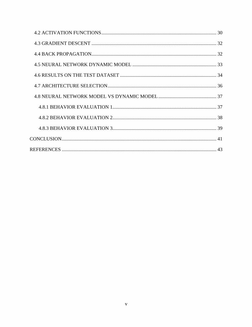
UUVSim. The UWSim is a kinematic simulator which is primarily used as a visualization tool [3].
UWSim has been used as a part of the Trident project and it renders high quality graphics with the
help of OpenSceneGraph (OSG) and osgOcean. The UUVSim package contains the
implementation of Gazebo plugins and ROS nodes necessary for the simulation of unmanned
underwater vehicles. The UUVSim plugin consists of several sensors and allows for simulating
the hydrodynamics of an AUV. For our purposes, UUVSim has the most applicable packages and
plugins required to simulate the underwater environment. Gazebo runs the UUVSim plugin as
shown below.
Figure 2 : UUVSim running on Gazebo
One of the key aspects in operating an autonomous vehicle is knowing its position with
respect to the environment. The process by which a vehicle can figure out where it is in the
environment is called localization and there are several methods applicable to the problem. One of
the most prominent localization techniques is using a Kalman filters [4]. The Kalman filter uses a
system model to predict the position of the vehicle. Romagos used a kinematic model of an
underwater vehicle to predict the system states [6]. The kinematic model deals with the motion of
the vehicle without taking the forces acting on the vehicle into account. It has been suggested the
use of a dynamic model instead of a kinematic model would yield better results in terms of
3
accuracy, since it considers the forces acting on the vehicle. Hascaryo has provided a detailed
derivation of the dynamic model and provided the preliminary results in his thesis [7]. This
research involves improving the work done by Hascaryo with the use of neural networks as an
alternative for modeling the dynamics of the underwater vehicle.
1.2 METHODOLOGY
Based on the work of Fossen, a dynamic model which has been observed to the de facto
standard has been implemented [2][8][9][10]. First, a generic 6 degrees of freedom (DoF) dynamic
model for an underwater vehicle was developed and then simplified into a 4 DoF model for
RexROV. 2 DoF were eliminated due to the inherent stability of the vehicle which helped in
reducing the 6x6 matrix to a pseudo 4x4 matrix thereby improving computing power. The 4 DoF
model incorporating the values derived by Berg [8], was used in the Extended Kalman filter (EKF)
equations and the output was used as input to a pure pursuit controller. The output of the dynamic
model was compared to the sensor values for verification. The pure pursuit controller provided the
steering angle required to drive the RexROV in a Robotic Operating System (ROS) Gazebo based
simulation environment, UUVSim [2]. Three behavior evaluation test courses, as suggested by
Norris [11], were used to evaluate the performance of kinematic and dynamic model driven
controllers.
The dynamic model required several coefficients, whose estimation can be difficult for real
time operations. A Neural Network based architecture in Tensor Flow [12] and Pytorch [13] was
developed to emulate the performance of the dynamic model. The fully connected network was
used to calculate the dynamic model values and fed to the Kalman filter and its performance was
compared with the dynamic model. The architecture was experimental, and several modifications
were made to improve the performance of the neural network based on the input parameters.
1.3 THESIS ORGANIZATION
This thesis was organized to demonstrate the performance of the dynamic model and how
Neural Networks can be used to overcome the drawbacks of a dynamic model. The introduction
chapter presents the motivation behind the research and the methodology. The research was
conducted on RexROV, a type of submarine, in a Gazebo based simulator called UUVSim.
Chapter 2 outlines the derivation of a generic dynamic model for an underwater vehicle.
The derivation was based on the “The Handbook of Marine Craft and Hydrodynamics” by Fossen.
4
The dynamic model was simplified for a RexROV and it was implemented in UUVSim. The results
of the dynamic model were compared with the IMU sensor values for evaluation.
Chapter 3 provides a brief introduction to the Kalman filter algorithm and the results of the
performance comparison between the dynamic model and the kinematic model on various test
courses using a pure pursuit controller. Chapter 4 demonstrates various Neural network
architectures that were used to model the dynamics of RexROV and their performance on various
test courses. Lastly the conclusion was provided in chapter 5. Future work and further
modifications to improve the performance of Neural Networks were suggested.
5
CHAPTER 2: DYNAMIC MODEL DERIVATION FOR RexROV
2.1 COORDINATE SYSTEMS AND CONVENTIONS
As discussed in the previous chapters, this research used the UUVSim based Gazebo
simulation environment. The simulation environment consisted of two bodies – the environment
(here it was the sea) and the vehicle. The environment was in North-East-Down (NED) frame [14]
while the vehicle was in BODY frame which follows the Society of Naval Architects and Marine
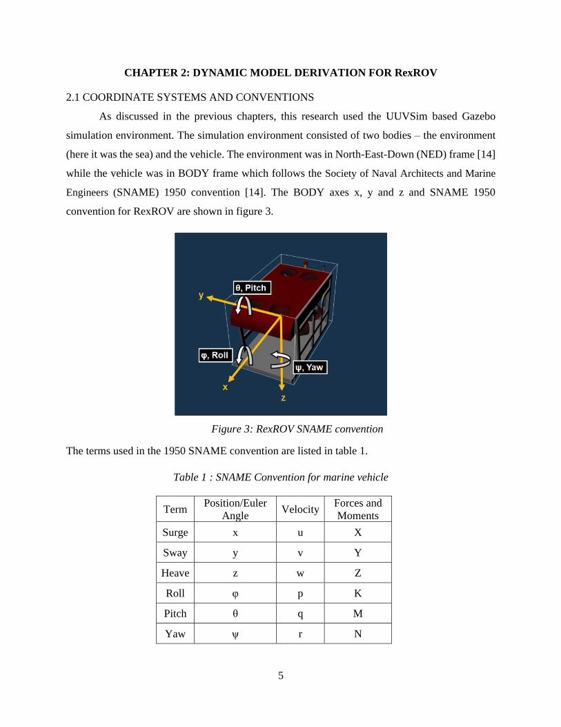
Engineers (SNAME) 1950 convention [14]. The BODY axes x, y and z and SNAME 1950
convention for RexROV are shown in figure 3.
Figure 3: RexROV SNAME convention
The terms used in the 1950 SNAME convention are listed in table 1.
Table 1 : SNAME Convention for marine vehicle
Term Position/Euler
Angle Velocity
Forces and
Moments
Surge x u X
Sway y v Y
Heave z w Z
Roll φ p K
Pitch θ q M
Yaw ψ r N
6
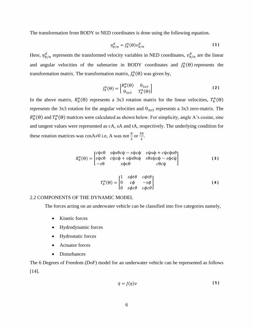
The transformation from BODY to NED coordinates is done using the following equation.
𝜂𝑏/𝑛𝑛 = 𝐽𝑏
𝑛(Θ)𝑣𝑏/𝑛𝑏 ( 1 )
Here, 𝜂𝑏/𝑛𝑛 represents the transformed velocity variables in NED coordinates, 𝑣𝑏/𝑛
𝑏 are the linear
and angular velocities of the submarine in BODY coordinates and 𝐽𝑏𝑛(Θ) represents the
transformation matrix. The transformation matrix, 𝐽𝑏𝑛(Θ) was given by,
𝐽𝑏𝑛(Θ) = [
𝑅𝑏𝑛(Θ) 03𝑥3
03𝑥3 𝑇𝑏𝑛(Θ)
] ( 2 )
In the above matrix, 𝑅𝑏𝑛(Θ) represents a 3x3 rotation matrix for the linear velocities, 𝑇𝑏
𝑛(Θ)
represents the 3x3 rotation for the angular velocities and 03𝑥3 represents a 3x3 zero-matrix. The
𝑅𝑏𝑛(Θ) and 𝑇𝑏
𝑛(Θ) matrices were calculated as shown below. For simplicity, angle A’s cosine, sine
and tangent values were represented as cA, sA and tA, respectively. The underlying condition for
these rotation matrices was cosA≠0 i.e, A was not π
2 or
3𝜋
2.
𝑅𝑏𝑛(Θ) = [
𝑐ψcθ 𝑠ϕsθcψ − 𝑠ψcϕ 𝑠ψsϕ + 𝑐ψcϕsθ𝑠ψcθ 𝑐ψcϕ + 𝑠ϕsθsψ 𝑠θsψcϕ − 𝑠ϕcψ−𝑠θ 𝑠ϕcθ 𝑐θcψ
] ( 3 )
𝑇𝑏𝑛(Θ) = [
1 𝑠𝜙𝑡𝜃 𝑐𝜙𝑡𝜃0 𝑐𝜙 −𝑠𝜙0 𝑠𝜙𝑐𝜃 𝑐𝜙𝑐𝜃
] ( 4 )
2.2 COMPONENTS OF THE DYNAMIC MODEL
The forces acting on an underwater vehicle can be classified into five categories namely,
• Kinetic forces
• Hydrodynamic forces
• Hydrostatic forces
• Actuator forces
• Disturbances
The 6 Degrees of Freedom (DoF) model for an underwater vehicle can be represented as follows
[14].
�� = 𝐽(𝜂)𝑣 ( 5 )
7
All of these forces were modeled separately and then added together to determine the dynamics of
the underwater vehicle.
𝑀�� + 𝐶(𝑣)𝑣 + 𝐷(𝑣)𝑣 + 𝑔(𝜂) + 𝑔0 = 𝜏 + 𝜏𝑤𝑖𝑛𝑑 + 𝜏𝑤𝑎𝑣𝑒 ( 6 )
The terms used in the equation were:
𝜂 - Vehicle position and pose
v - Vehicle velocity
J - Transformation matrix between NED and BODY coordinate systems
M - inertial matrix
C(v) - Coriolis forces
D(v) - Damping matrix
g(𝜂) - Buoyancy force
𝜏, 𝜏𝑤𝑖𝑛𝑑 𝑎𝑛𝑑 𝜏𝑤𝑎𝑣𝑒 – Actuator, Wind and Wave forces respectively.
2.2.1 KINETIC FORCES
The underwater vehicle was considered as a rigid body and it does not undergo any
deformation during its operation. For the purpose of simplicity, it was assumed that the center of
mass coincided with the center of gravity (CG). The kinetic force was the force required to move
the submarine from its state of rest. The kinetic force (τ𝑅𝐵) consisted of the inertial component
(𝑀𝑅𝐵) and Coriolis component (𝐶𝑅𝐵(𝑣)) as shown. Here the subscript RB represents rigid body.
τ𝑅𝐵 = 𝑀𝑅𝐵�� + 𝐶𝑅𝐵(𝑣)v ( 7 )
Here v and �� represent the velocity and acceleration vectors. The velocity and acceleration vectors
comprise both the linear and angular components as shown.

8
v =
[ 𝑢𝑣𝑤𝑝𝑞𝑟 ]
( 8 )
v =
[ ������������ ]
( 9 )
Newton’s first law of motion defines inertia as the tendency of the body to remain in its state of
rest or of uniform motion unless an external force acts on it to change its state. The inertial
component for a rigid body with 6 DoF was represented as shown below.
𝑀𝑅𝐵 =
[ 𝑚 0 0 0 0 00 𝑚 0 0 0 00 0 𝑚 0 0 00 0 0 𝐼𝑥𝑥 𝐼𝑥𝑦 𝐼𝑥𝑧
0 0 0 𝐼𝑥𝑦 𝐼𝑦𝑦 𝐼𝑦𝑧
0 0 0 𝐼𝑥𝑧 𝐼𝑦𝑧 𝐼𝑧𝑧]
( 10 )
Coriolis effect was the effect experience by a moving body in a rotating system and it acts
perpendicular to the direction of motion and towards the center of rotation. The Coriolis
component for an underwater vehicle was given below.
𝐶𝑅𝐵(𝑣) = [𝑚𝑆(𝑣2) −𝑚𝑆(𝑣2)𝑆(𝑟𝑔
𝑏)
𝑚𝑆(𝑟𝑔𝑏)𝑆(𝑣2) −𝑆(𝐼𝑏𝑣2)
] ( 11 )
Here 𝑆 represents the skew matrix, 𝑣2 represents the vessel velocity vector and 𝐼𝑏 represents the
moment of inertia matrix. Since the center of mass coincides with the center of gravity, the skew
matrix (𝑆(𝑟𝑔𝑏) for the CG vector becomes null. This yield, 𝐶𝑅𝐵(𝑣)𝑣 as shown below [9].
𝐶𝑅𝐵(𝑣)v = −
[ 𝑚(𝑞𝑤 − 𝑟𝑣)
𝑚(𝑟𝑢 − 𝑝𝑤)
𝑚(𝑝𝑣 − 𝑞𝑢)
𝑞𝑟(𝐼𝑦𝑦 − 𝐼𝑧𝑧)
𝑟𝑝(𝐼𝑧𝑧 − 𝐼𝑧𝑧)
𝑞𝑝(𝐼𝑥𝑥 − 𝐼𝑦𝑦)]
( 12 )
9
2.2.2 HYDRODYNAMIC FORCES
The hydrodynamic forces include three components: the hydrodynamic drag (D(𝑣)v),
Coriolis-centripetal force (𝐶𝐴(𝑣)v) and inertial force (𝑀𝐴��). This was represented as,
τℎ𝑦𝑑𝑟𝑜𝑑𝑦𝑛𝑎𝑚𝑖𝑐𝑠 = −D(𝑣)v − 𝐶𝐴(𝑣)v − 𝑀𝐴�� ( 13 )
The hydrodynamic drag was the damping force acting on the body and was comprised of linear
and quadratic drag as shown.
D(𝑣) = 𝐷𝑙𝑖𝑛𝑒𝑎𝑟 + 𝐷𝑞𝑢𝑎𝑑𝑟𝑎𝑡𝑖𝑐 ( 14 )
Where 𝐷𝑙𝑖𝑛𝑒𝑎𝑟 and 𝐷𝑞𝑢𝑎𝑑𝑟𝑎𝑡𝑖𝑐 were diagonal matrices comprising of the linear and quadratic
damping components respectively. Adding the two matrices and multiplying them with the
velocity vector gives the damping force as shown.
D(𝑣) = −
[ (𝑋𝑢 + 𝑋𝑢|𝑢||𝑢|)𝑢
(𝑌𝑣 + 𝑌𝑣|𝑣||𝑣|)𝑣
(𝑍𝑤 + 𝑍𝑤|𝑤||𝑤|)𝑤
(𝐾𝑝 + 𝐾𝑝|𝑝||𝑝|)𝑝
(𝑀𝑞 + 𝑀𝑞|𝑞||𝑞|)𝑞
(𝑁𝑟 + 𝑁𝑟|𝑟||𝑟|)𝑟 ]
( 15 )
The Coriolis-centripetal force (𝐶𝐴(𝑣)v) and inertial force (𝑀𝐴��) were obtained from Fossen [15]
using the low speed assumption as shown below.
𝐶𝐴(𝑣)v = −
[
𝑌��𝑣𝑟 − 𝑍��𝑤𝑞𝑍��𝑤𝑝 − 𝑋��𝑢𝑟𝑋��𝑢𝑞 − 𝑌��𝑣𝑝
(𝑌�� − 𝑍��)𝑣𝑤 + (𝑀�� − 𝑁��)𝑞𝑟
(𝑍�� − 𝑋��)𝑢𝑤 + (𝑁�� − 𝐾��)𝑝𝑟
(𝑋�� − 𝑌��)𝑢𝑣 + (𝐾�� − 𝑀��)𝑝𝑞 ]
( 16 )
10
𝑀𝐴�� =
[ 𝑋����𝑌����𝑍����𝐾����
𝑀����
𝑁���� ]
( 17 )
2.2.3 HYDROSTATIC FORCES
The hydrostatic forces consisted of two forces: buoyancy and gravitational force(weight).
It was assumed that the Center of Buoyancy (CB) and Center of Gravity (CG) were on the z-axis
and zB was the distance of the CB to the CG for simplicity as the assumption holds for most of the
cases. Buoyancy was the upward force caused when immersing a body into a liquid and was a
factor of the volume of the liquid displaced by the body. In the case of a fully submerged vehicle
(AUV), the volume of liquid displaced was equal to the total volume of the vehicle. Hence
buoyancy (B) and the weight (W) of the vehicle, are as shown.
B = ρgV ( 18 )
W = mg ( 19 )
Here, ρ was the density of water and V was the volume of the vehicle. The sum of the two forces
gives the hydrostatic force (g(η)) which in vector form was as shown.
g(η) = −
[
−(𝑊 − 𝐵) sin θ(𝑊 − 𝐵) cos θ sinϕ(𝑊 − 𝐵) cos θ cosϕ
𝑧𝐵 cos θ sinϕ𝑧𝐵 sin θ
0 ]
( 20 )
2.2.4 THRUSTER FORCES
The final component of the dynamic model involves the thruster forces and other
disturbances. Deep underwater, the effects of wind and ocean currents were minimal and hence
𝜏𝑤𝑖𝑛𝑑 and 𝜏𝑤𝑎𝑣𝑒 were equivalent to zero. The thrust forces were the vector sum of the individual
thruster forces in the respective axes and given by,
11
𝑇𝑖 =
[ 𝑇𝑥
𝑇𝑦
𝑇𝑧
𝑇ϕ
𝑇θ
𝑇ψ]
( 21 )
2.3 DYNAMIC MODEL DERIVATION
Substituting the individual components into the equation 6 and decomposing them to their
corresponding acceleration components, we have the dynamic model as follows:
�� = (1
𝑚 − 𝑋��) ((𝑋𝑢 + 𝑋𝑢|𝑢||𝑢|)u + (𝐵 − 𝑊) sin θ + m(𝑟𝑣 − 𝑞𝑤) − 𝑌��rv + 𝑍��qw
+ 𝑇𝑥)
( 22 )
�� = (1
𝑚 − 𝑌��) ((𝑌𝑣 + 𝑌𝑣|𝑣||𝑣|)v − (𝐵 − 𝑊) sinϕ cos θ + m(𝑝𝑤 − 𝑟𝑢) − 𝑋��ru
+ 𝑍��pw + 𝑇𝑦)
( 23 )
w = (1
m − Zw) ((Zw + Zw|w||w|)w − (B − W) cos θ cosϕ + m(qu − pv) − Xuqu
+ Yvpv + Tz)
( 24 )
�� = (1
𝐼𝑥 − 𝐾��) ((𝐾𝑝 + 𝐾𝑝|𝑝||𝑝|)p − (𝑀�� − 𝑁��)qr + (𝐼𝑦𝑦 − 𝐼𝑧𝑧)qr + (𝑍�� − 𝑌��)vw
+ B𝑧𝐵 cos θ sinϕ + 𝑇θ)
( 25 )
�� = (1
𝐼𝑦 − 𝑀��) ((𝑀𝑞 + 𝑀𝑞|𝑞||𝑞|)q − (𝑁�� − 𝐾��)pr + (𝐼𝑧𝑧 − 𝐼𝑦𝑦)pr + (𝑋�� − 𝑍��)uw
+ B𝑧𝐵 sin θ + 𝑇ϕ)
( 26 )
12
�� = (1
𝐼𝑧 − 𝑁��) ((𝑁𝑟 + 𝑁𝑟|𝑟||𝑟|)r − (𝐾�� − 𝑀��)pq + (𝐼𝑥𝑥 − 𝐼𝑦𝑦)pq + (𝑌�� − 𝑋��)uv
+ 𝑇ψ)
( 27 )
These six dynamic equations were generic to an underwater vehicle with 6 DoF. For our purpose,
we modified them based on the configuration of the RexROV before using them in the Extended
Kalman Filter.
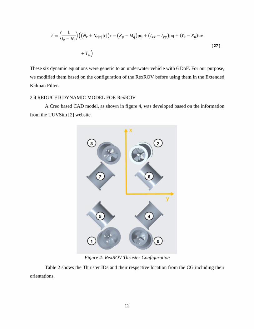
2.4 REDUCED DYNAMIC MODEL FOR RexROV
A Creo based CAD model, as shown in figure 4, was developed based on the information
from the UUVSim [2] website.
Figure 4: RexROV Thruster Configuration
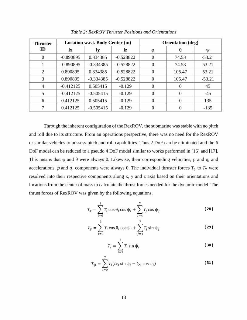
Table 2 shows the Thruster IDs and their respective location from the CG including their
orientations.
13
Table 2: RexROV Thruster Positions and Orientations
Thruster
ID
Location w.r.t. Body Center (m) Orientation (deg)
lx ly lz φ θ ψ
0 -0.890895 0.334385 -0.528822 0 74.53 -53.21
1 -0.890895 -0.334385 -0.528822 0 74.53 53.21
2 0.890895 0.334385 -0.528822 0 105.47 53.21
3 0.890895 -0.334385 -0.528822 0 105.47 -53.21
4 -0.412125 0.505415 -0.129 0 0 45
5 -0.412125 -0.505415 -0.129 0 0 -45
6 0.412125 0.505415 -0.129 0 0 135
7 0.412125 -0.505415 -0.129 0 0 -135
Through the inherent configuration of the RexROV, the submarine was stable with no pitch
and roll due to its structure. From an operations perspective, there was no need for the RexROV
or similar vehicles to possess pitch and roll capabilities. Thus 2 DoF can be eliminated and the 6
DoF model can be reduced to a pseudo 4 DoF model similar to works performed in [16] and [17].
This means that φ and θ were always 0. Likewise, their corresponding velocities, p and q, and
accelerations, �� and ��, components were always 0. The individual thruster forces 𝑇0 to 𝑇7 were
resolved into their respective components along x, y and z axis based on their orientations and
locations from the center of mass to calculate the thrust forces needed for the dynamic model. The
thrust forces of RexROV was given by the following equations.
𝑇𝑥 = ∑𝑇𝑖 cos θ𝑖 cosψ𝑖
3
𝑖=0
+ ∑𝑇𝑗 cosψ𝑗
7
𝑗=4
( 28 )
𝑇𝑦 = ∑𝑇𝑖 cos θ𝑖 cosψ𝑖
3
𝑖=0
+ ∑𝑇𝑗 sinψ𝑗
7
𝑗=4
( 29 )
𝑇𝑧 = ∑𝑇𝑖 sinψ𝑖
3
𝑖=1
( 30 )
𝑇ψ = ∑𝑇𝑖(𝑙𝑥𝑖 sinψ𝑖 − 𝑙𝑦𝑖 cosψ𝑖)
7
𝑖=0
( 31 )
14
The dynamic model for RexROV reduced to the following set of equations (32) to (35).
�� = (1
𝑚 − 𝑋��) ((𝑋𝑢 + 𝑋𝑢|𝑢||𝑢|)u + mrv − 𝑌��rv + 𝑇𝑥) ( 32 )
�� = (1
𝑚 − 𝑌��) ((𝑌𝑣 + 𝑌𝑣|𝑣||𝑣|)v + mru + 𝑋��ru + 𝑇𝑦) ( 33 )
�� = (1
𝑚−𝑍��) ((𝑍𝑤 + 𝑍𝑤|𝑤||𝑤|)𝑤 − (𝐵 − 𝑊) + 𝑇𝑧) ( 34 )
�� = (1
𝐼𝑧 − 𝑁��) ((𝑁𝑟 + 𝑁𝑟|𝑟||𝑟|)r + (𝑌�� − 𝑋��)uv + 𝑇ψ) ( 35 )
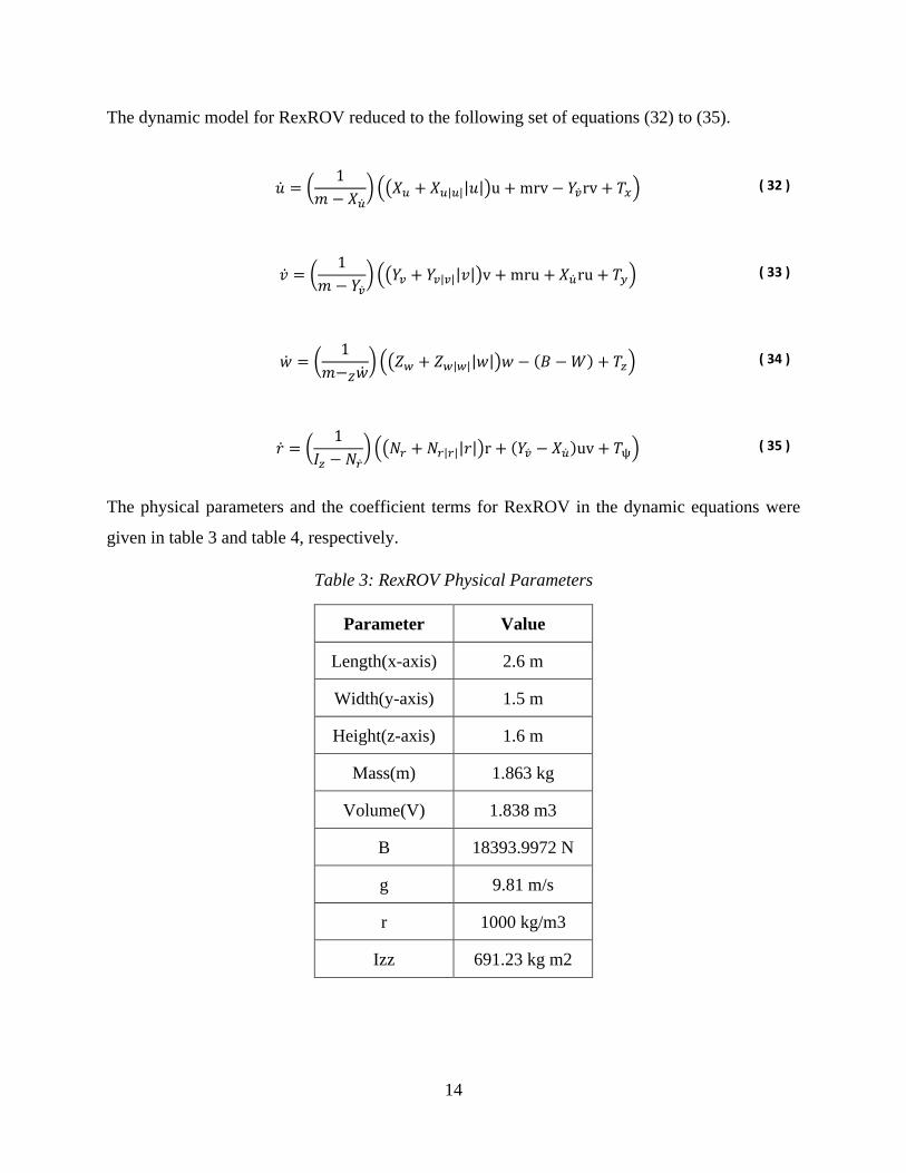
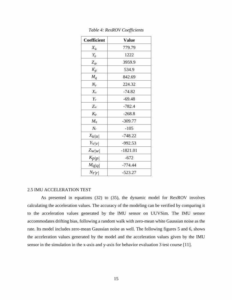
The physical parameters and the coefficient terms for RexROV in the dynamic equations were
given in table 3 and table 4, respectively.
Table 3: RexROV Physical Parameters
Parameter Value
Length(x-axis) 2.6 m
Width(y-axis) 1.5 m
Height(z-axis) 1.6 m
Mass(m) 1.863 kg
Volume(V) 1.838 m3
B 18393.9972 N
g 9.81 m/s
r 1000 kg/m3
Izz 691.23 kg m2
15
Table 4: RexROV Coefficients
Coefficient Value
𝑋�� 779.79
𝑌�� 1222
𝑍�� 3959.9
𝐾�� 534.9
𝑀�� 842.69
𝑁�� 224.32
Xu -74.82
Yv -69.48
Zw -782.4
Kp -268.8
Mq -309.77
Nr -105
Xu|u| -748.22
Yv|v| -992.53
Zw|w| -1821.01
Kp|p| -672
Mq|q| -774.44
Nr|r| -523.27
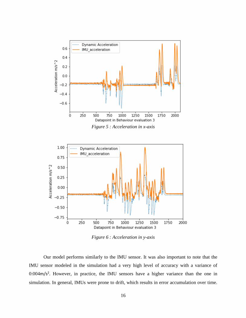
2.5 IMU ACCELERATION TEST
As presented in equations (32) to (35), the dynamic model for RexROV involves
calculating the acceleration values. The accuracy of the modeling can be verified by comparing it
to the acceleration values generated by the IMU sensor on UUVSim. The IMU sensor
accommodates drifting bias, following a random walk with zero-mean white Gaussian noise as the
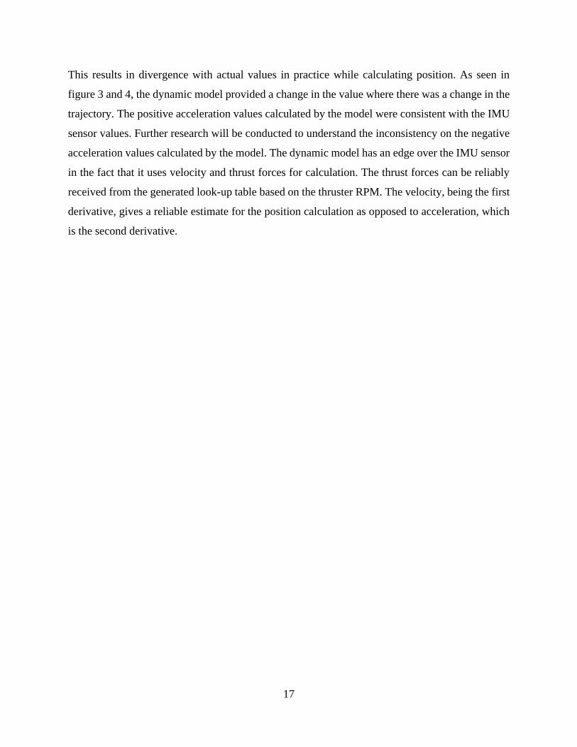
rate. Its model includes zero-mean Gaussian noise as well. The following figures 5 and 6, shows
the acceleration values generated by the model and the acceleration values given by the IMU
sensor in the simulation in the x-axis and y-axis for behavior evaluation 3 test course [11].
16
Figure 5 : Acceleration in x-axis
Figure 6 : Acceleration in y-axis
Our model performs similarly to the IMU sensor. It was also important to note that the
IMU sensor modeled in the simulation had a very high level of accuracy with a variance of
0:004m/s2. However, in practice, the IMU sensors have a higher variance than the one in
simulation. In general, IMUs were prone to drift, which results in error accumulation over time.
17
This results in divergence with actual values in practice while calculating position. As seen in
figure 3 and 4, the dynamic model provided a change in the value where there was a change in the
trajectory. The positive acceleration values calculated by the model were consistent with the IMU
sensor values. Further research will be conducted to understand the inconsistency on the negative
acceleration values calculated by the model. The dynamic model has an edge over the IMU sensor
in the fact that it uses velocity and thrust forces for calculation. The thrust forces can be reliably
received from the generated look-up table based on the thruster RPM. The velocity, being the first
derivative, gives a reliable estimate for the position calculation as opposed to acceleration, which
is the second derivative.

18
CHAPTER 3: COMPARISION OF DYNAMIC AND KINEMATIC KALMAN FILTER
3.1 KALMAN FILTERS
Kalman filter-based localization techniques have been prevalent since the 1960s [4]. The
Kalman Filter was an iterative mathematical tool used to estimate the position of a system based
on a system of equations and measurements. The Kalman filter has three steps namely
Initialization, Prediction and Update step.
Initialization: Initialize the state of the filter and the belief in the state
Prediction:
1. Use the process model to predict the state of the system in the next time step
2. Adjust belief to account for uncertainty in prediction
Update:
1. Get a measurement from the sensor and associated belief about its accuracy
2. Compute residual between predicted state and measurement
3. Compute Kalman Gain based on whether the measurement or prediction was more accurate
4. Set state between the prediction and measurement based on scaling factor
5. Update belief in the state based on how certain we were in the measurement
Initialization was a one-time process while the prediction and update were iterative. The Kalman
filter has two major conditions in order to work:
1. The Kalman Filter works with Gaussian Distribution
2. The prediction and the update equations were linear
These two conditions go hand in hand. A linear system fed to a gaussian produces a
gaussian output while a nonlinear system produces a non-gaussian output. Hence Kalman Filters
work well with linear systems of equations. However, most of the real-time systems that we
encounter were often nonlinear. One way to apply a Kalman Filter to these non-linear systems was
to approximate them to linear systems using Taylor series around the mean of the nonlinear
Gaussian. This version of the Kalman filter is referred to as the Extended Kalman filter (EKF).
While the equations remain the same from the Kalman Filter, one major change was that we used
the Gauss Jacobian Matrix instead of the State transition matrix for linear approximations. At each
19
time step, the Jacobian was evaluated with current predicted states. These matrices were used in
the Kalman filter equations. This process linearizes the nonlinear function around the current
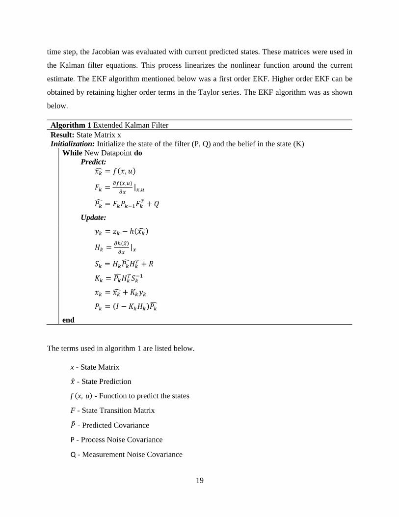
estimate. The EKF algorithm mentioned below was a first order EKF. Higher order EKF can be
obtained by retaining higher order terms in the Taylor series. The EKF algorithm was as shown
below.
Algorithm 1 Extended Kalman Filter
Result: State Matrix x
Initialization: Initialize the state of the filter (P, Q) and the belief in the state (K)
While New Datapoint do
Predict:
𝑥�� = 𝑓(𝑥, 𝑢)
𝐹𝑘 =𝜕𝑓(𝑥,𝑢)
𝜕𝑥|𝑥,𝑢
𝑃�� = 𝐹𝑘𝑃𝑘−1𝐹𝑘𝑇 + 𝑄
Update:
𝑦𝑘 = 𝑧𝑘 − ℎ(𝑥��)
𝐻𝑘 =𝜕ℎ(��)
𝜕𝑥|𝑥
𝑆𝑘 = 𝐻𝑘𝑃��𝐻𝑘𝑇 + 𝑅
𝐾𝑘 = 𝑃��𝐻𝑘𝑇𝑆𝑘
−1
𝑥𝑘 = 𝑥�� + 𝐾𝑘𝑦𝑘
𝑃𝑘 = (𝐼 − 𝐾𝑘𝐻𝑘)𝑃��
end
The terms used in algorithm 1 are listed below.
x - State Matrix
�� - State Prediction
f (x, u) - Function to predict the states
F - State Transition Matrix
�� - Predicted Covariance
P - Process Noise Covariance
Q - Measurement Noise Covariance

20
z - Measurement from Sensors
h(��) - Prediction to Measurement coordinate
y - Difference between Prediction and Measurement
H - Jacobian Matrix
R - Measurement Noise Covariance
K - Kalman Gain
I - Identity Matrix
k - Represents the current time step
k-1 - Represents the previous time step
Another version of Kalman filter that exists was the Unscented Kalman Filter (UKF. A
UKF differs from an EKF in that it takes a defined set of multiple points from the nonlinear system,
including the mean, for approximation while an EKF considers only the mean to approximate the
system [5]. Thus, UKF offers a better approximation of the non-linear system than the EKF. The
defined set of multiple points were called the sigma points and each of these points have a weight
associated with them. The sigma points were representative of the whole distribution. The number
of sigma points taken per dimension was given by (2N+1), where N was the number of dimensions
of the system. After selecting the sigma points, the weights associated with each of the points were
calculated. These points were then transformed using a nonlinear function. The gaussian of the
resulting transformed points were calculated and its mean and variance are computed. This method
is known as the Unscented method. To summarize, the Unscented method consists of the following
five steps:
1. Compute Set of Sigma Points
2. Assign Weights to each sigma point
3. Transform the points through nonlinear function
4. Compute Gaussian from weighted and transformed points
5. Compute Mean and Variance of the new Gaussian.
While taking all the points from the nonlinear system would give a better approximation
compared to taking a defined set of points, the method fails in terms of computation power and
optimality. So, for our purposes, the Extended Kalman filter was used. The EKF uses a process
model to predict the system states.
21
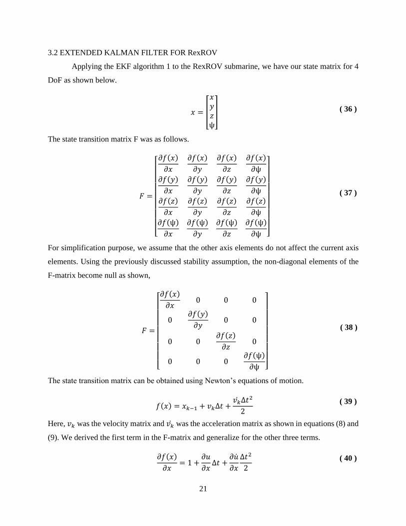
3.2 EXTENDED KALMAN FILTER FOR RexROV
Applying the EKF algorithm 1 to the RexROV submarine, we have our state matrix for 4
DoF as shown below.
𝑥 = [
𝑥𝑦𝑧ψ
] ( 36 )
The state transition matrix F was as follows.
𝐹 =
[ ∂𝑓(𝑥)
∂𝑥
∂𝑓(𝑥)
∂𝑦
∂𝑓(𝑥)
∂𝑧
∂𝑓(𝑥)
∂ψ
∂𝑓(𝑦)
∂𝑥
∂𝑓(𝑦)
∂𝑦
∂𝑓(𝑦)
∂𝑧
∂𝑓(𝑦)
∂ψ
∂𝑓(𝑧)
∂𝑥
∂𝑓(𝑧)
∂𝑦
∂𝑓(𝑧)
∂𝑧
∂𝑓(𝑧)
∂ψ
∂𝑓(ψ)
∂𝑥
∂𝑓(ψ)
∂𝑦
∂𝑓(ψ)
∂𝑧
∂𝑓(ψ)
∂ψ ]
( 37 )
For simplification purpose, we assume that the other axis elements do not affect the current axis
elements. Using the previously discussed stability assumption, the non-diagonal elements of the
F-matrix become null as shown,
𝐹 =
[ ∂𝑓(𝑥)
∂𝑥0 0 0
0∂𝑓(𝑦)
∂𝑦0 0
0 0∂𝑓(𝑧)
∂𝑧0
0 0 0∂𝑓(ψ)
∂ψ ]
( 38 )
The state transition matrix can be obtained using Newton’s equations of motion.
𝑓(𝑥) = 𝑥𝑘−1 + 𝑣𝑘Δ𝑡 +𝑣��Δ𝑡2
2
( 39 )
Here, 𝑣𝑘 was the velocity matrix and 𝑣�� was the acceleration matrix as shown in equations (8) and
(9). We derived the first term in the F-matrix and generalize for the other three terms.
∂𝑓(𝑥)
∂𝑥= 1 +
∂𝑢
∂𝑥Δ𝑡 +
∂��
∂𝑥
Δ𝑡2
2
( 40 )
22
∂𝑓(𝑥)
∂𝑥= 1 +
∂𝑢
∂𝑡
∂𝑡
∂𝑥Δ𝑡 +
∂��
∂𝑡
∂𝑡
∂𝑥
Δ𝑡2
2
( 41 )
The filter we were considering for the simulation worked at a frequency of 10Hz. For such a small
change in time, the partial derivative term was taken as shown below.
∂𝑓(𝑥)
∂𝑥= 1 + ��
1
𝑢Δ𝑡 +
��
Δ𝑡
1
𝑢
Δ𝑡2
2
( 42 )
This can be further simplified to,
∂𝑓(𝑥)
∂𝑥= 1 +
��
𝑢Δ𝑡 +
Δ��Δ𝑡
2𝑢
( 43 )
Similarly, the other three terms for the F-matrix were derived.
∂𝑓(𝑦)
∂𝑦= 1 +
��
𝑣Δ𝑡 +
Δ��Δ𝑡
2𝑣
( 44 )
∂𝑓(𝑧)
∂𝑧= 1 +
��
𝑤Δ𝑡 +
Δ��Δ𝑡
2𝑤
( 45 )
∂𝑓(ψ)
∂ψ= 1 +
��
𝑟Δ𝑡 +
Δ��Δ𝑡
2𝑟 ( 46 )
In the simulation, the velocity values were obtained from the Doppler Velocity Log (DVL) sensor
while the acceleration values were obtained from the Inertial Measurement Unit (IMU) sensor.
The Global Positioning System (GPS) sensor provided the x and y measurements. The pressure
sensor gave the z measurements and the compass built into the IMU sensor gave the ψ update. It
was important to note that both the predictions (ℎ(��)) and the measurements (��) were in the same
coordinates. This rendered the Jacobian matrix (H) as an Identity matrix of size 4.
𝐻 =∂ℎ(��)
∂��=
∂��
∂��= 𝐼4
( 47 )
The update equation was further simplified as shown.
𝑆𝑘 = 𝑃�� + 𝑅 ( 48 )
𝐾𝑘 = 𝑃��𝑆𝑘−1 ( 49 )
23
𝑥𝑘 = 𝑥�� + 𝐾𝑘𝑦𝑘 ( 50 )
𝑃𝑘 = (𝐼 − 𝐾𝑘)𝑃�� ( 51 )
The Extended Kalman filter algorithm for RexROV after applying the simplifications is shown
below.
Algorithm 1 Extended Kalman Filter for RexROV
Result: State Matrix x
Initialization: Initialize the state of the filter (P, Q) and the belief in the state (K)
While New Datapoint do
Predict:
𝑥�� = 𝑓(𝑥, 𝑢)
𝐹𝑘 =𝜕𝑓(𝑥,𝑢)
𝜕𝑥|𝑥,𝑢
𝑃�� = 𝐹𝑘𝑃𝑘−1𝐹𝑘𝑇 + 𝑄
Update:
𝑦𝑘 = 𝑧𝑘 − (𝑥��)
𝐻𝑘 =𝜕ℎ(��)
𝜕𝑥|𝑥
𝑆𝑘 = 𝑃�� + 𝑅
𝐾𝑘 = 𝑃��𝑆𝑘−1
𝑥𝑘 = 𝑥�� + 𝐾𝑘𝑦𝑘
𝑃𝑘 = (𝐼 − 𝐾𝑘)𝑃��
end
The following algorithm was implemented in real-time in UUVSim and the Kalman filter
prediction values were used in a pure pursuit controller implemented by the Submarine Bois team
to drive the submarine on a predetermined path [11].
3.3 PURE PURSUIT CONTROLLER
For a given set of waypoints, a pure pursuit algorithm approaches the target waypoint
ignoring the dynamics/kinematics of the environment and the vehicle (except vehicle length). Once
24
in the vicinity (user defined) of the target waypoint, the algorithm generates the steering command
for the next waypoint until the system reaches the last waypoint [25]. For our purposes, we were
generated the steering command while the linear velocity remained constant.
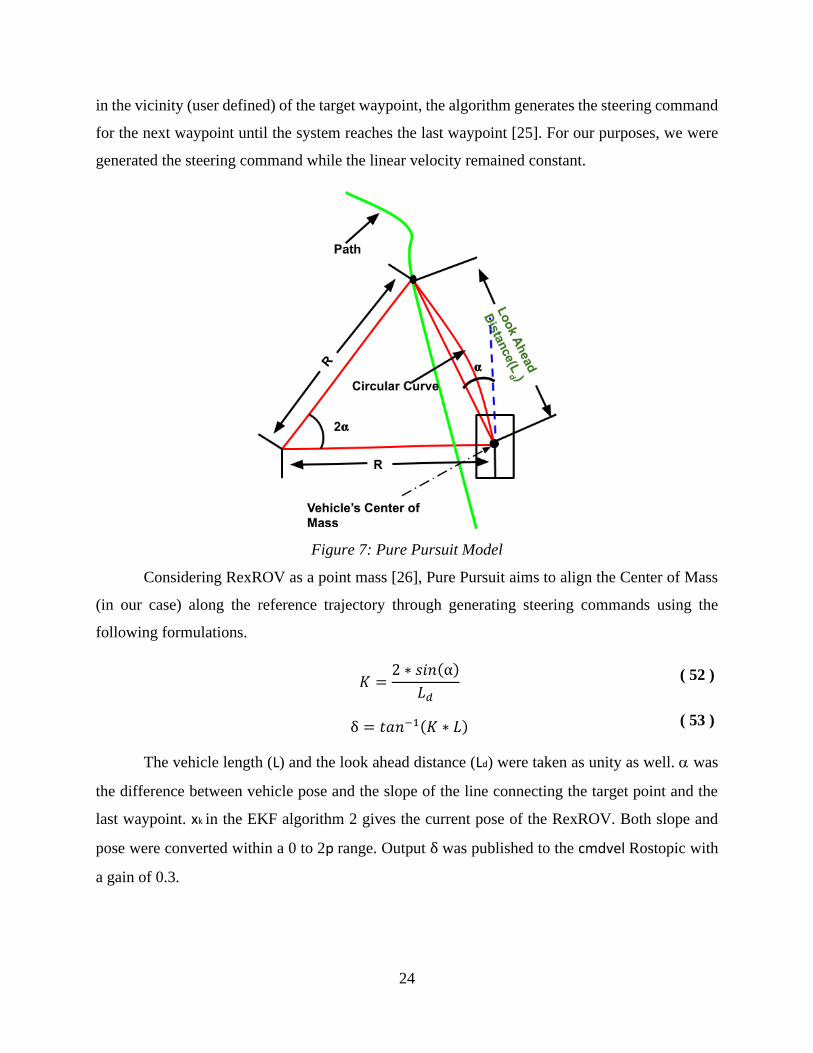
Figure 7: Pure Pursuit Model
Considering RexROV as a point mass [26], Pure Pursuit aims to align the Center of Mass
(in our case) along the reference trajectory through generating steering commands using the
following formulations.
𝐾 =2 ∗ 𝑠𝑖𝑛(α)
𝐿𝑑 ( 52 )
δ = 𝑡𝑎𝑛−1(𝐾 ∗ 𝐿) ( 53 )
The vehicle length (L) and the look ahead distance (Ld) were taken as unity as well. was
the difference between vehicle pose and the slope of the line connecting the target point and the
last waypoint. xk in the EKF algorithm 2 gives the current pose of the RexROV. Both slope and
pose were converted within a 0 to 2p range. Output δ was published to the cmdvel Rostopic with
a gain of 0.3.
25
3.4 TEST COURSES
In this section, the performance of the kinematic and the dynamic model driven pure pursuit
controllers were compared on various test courses adopted from [11]. The figure shows the actual
path followed by the vehicle as opposed to the output of the dynamic model and kinematic model.
The results from the test courses were summarized as a table. Total was the mean of the Cartesian
distance between the reference path and the path taken by the RexROV when using the controllers.
X-Kalman gives the mean squared error (MSE) between the value predicted by the Kalman filter
and the actual path traced by the RexROV. Likewise, Y-Kalman gives MSE on the y-axis.
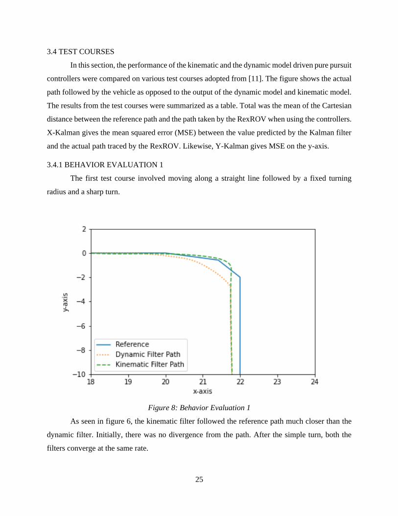
3.4.1 BEHAVIOR EVALUATION 1
The first test course involved moving along a straight line followed by a fixed turning
radius and a sharp turn.
Figure 8: Behavior Evaluation 1
As seen in figure 6, the kinematic filter followed the reference path much closer than the
dynamic filter. Initially, there was no divergence from the path. After the simple turn, both the
filters converge at the same rate.
26
Table 5: Results of Behavior Evaluation 1
Error Dynamic Filter Kinematic Filter
Total 0.1166m 0.09880m
X-Kalman 0.0825m 0.3432m
Y-Kalman 0.2665m 1.024m
From table 5, the total error of the kinematic filter was less than the dynamic filter.
However, this was attributed to the controller and not the filter itself as it can be inferred from the
other two entries in the table. To make further assessment of the filters, they were tested on the
behavior evaluation 2 test course.
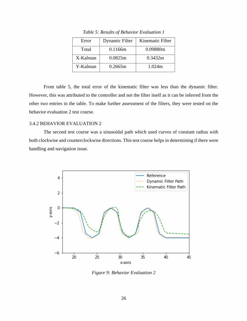
3.4.2 BEHAVIOR EVALUATION 2
The second test course was a sinusoidal path which used curves of constant radius with
both clockwise and counterclockwise directions. This test course helps in determining if there were
handling and navigation issue.
Figure 9: Behavior Evaluation 2
27
As seen in figure 7, the dynamic filter does a much better job than the kinematic filter when
tracing a curve. The dynamic filter converged faster when there was a change in both x and y co-
ordinates.
Table 6 : Results of Behavior Evaluation 2
Error Dynamic Filter Kinematic Filter
Total 0.1659m 0.2482m
X-Kalman 0.1213m 0.39145m
Y-Kalman 0.3682m 4.336m
From table 6, the mean error of the dynamic filter was less than the kinematic filter. The
dynamic filter handled the simultaneous changes in the x-axis and y-axis much better than the
kinematic filter.
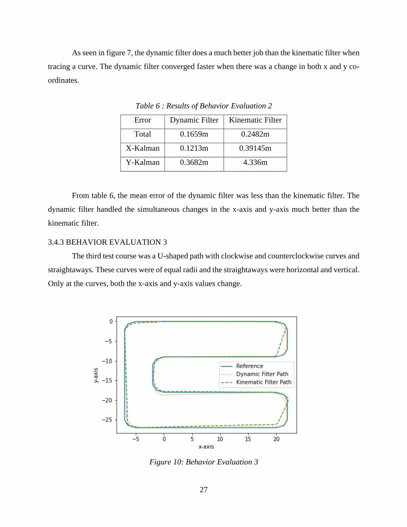
3.4.3 BEHAVIOR EVALUATION 3
The third test course was a U-shaped path with clockwise and counterclockwise curves and
straightaways. These curves were of equal radii and the straightaways were horizontal and vertical.
Only at the curves, both the x-axis and y-axis values change.
Figure 10: Behavior Evaluation 3
28
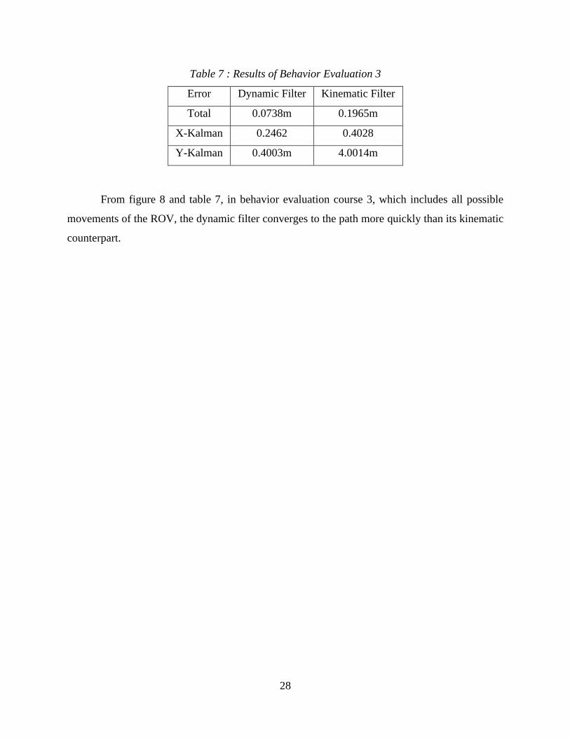
Table 7 : Results of Behavior Evaluation 3
Error Dynamic Filter Kinematic Filter
Total 0.0738m 0.1965m
X-Kalman 0.2462 0.4028
Y-Kalman 0.4003m 4.0014m
From figure 8 and table 7, in behavior evaluation course 3, which includes all possible
movements of the ROV, the dynamic filter converges to the path more quickly than its kinematic
counterpart.
29
CHAPTER 4: NEURAL NETWORK DYNAMIC MODEL
4.1 MULTI-LAYER NEURAL NETWORKS
Neural networks have been used to make classifications, predictions and a variety of other
applications [18][19]. Neural networks have an input later and an output layer. The layers in
between the input and output layers were referred to as hidden layers. Depending on the number
of hidden layers used, they can be classified as shallow and deep neural networks. Like any
machine learning algorithm, the neural network takes in a set of inputs and a set of target values
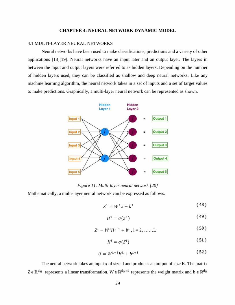
to make predictions. Graphically, a multi-layer neural network can be represented as shown.
Figure 11: Multi-layer neural network [20]
Mathematically, a multi-layer neural network can be expressed as follows.
𝑍1 = 𝑊1𝑥 + 𝑏1 ( 48 )
𝐻1 = 𝜎(𝑍1) ( 49 )
𝑍𝑙 = 𝑊𝑙𝐻𝑙−1 + 𝑏𝑙 , l = 2, ……L ( 50 )
𝐻𝑙 = 𝜎(𝑍𝑙) ( 51 )
𝑈 = 𝑊𝐿+1𝐻𝐿 + 𝑏𝐿+1 ( 52 )
The neural network takes an input x of size d and produces an output of size K. The matrix
Z ϵ ℝdH represents a linear transformation. W ϵ ℝdHxd represents the weight matrix and b ϵ ℝdH
30
was the bias matrix. dH was the dimension of the hidden layer. To learn the model, an element-
wise nonlinearity 𝜎(−) : ℝ → ℝ was applied to each element of matrix Z to obtain the hidden
layer H ϵ ℝdH. L was the number of hidden layers. 𝑈 ϵ ℝ𝐾 represents the output layer.
4.2 ACTIVATION FUNCTIONS
The common choices for the nonlinear activation functions, 𝜎(−) were:
Sigmoid - σ(𝑥) =𝑒𝑧
1 + 𝑒𝑧
Tanh() - σ(𝑥) =𝑒𝑥 − 𝑒−𝑥
𝑒𝑥 + 𝑒−𝑥
Rectified Linear Units (ReLU) - σ(𝑥) = 𝑚𝑎𝑥(𝑥, 0)
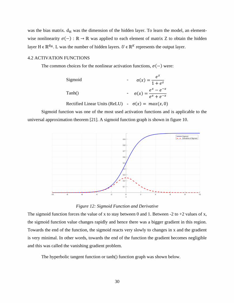
Sigmoid function was one of the most used activation functions and is applicable to the
universal approximation theorem [21]. A sigmoid function graph is shown in figure 10.
Figure 12: Sigmoid Function and Derivative
The sigmoid function forces the value of x to stay between 0 and 1. Between -2 to +2 values of x,
the sigmoid function value changes rapidly and hence there was a bigger gradient in this region.
Towards the end of the function, the sigmoid reacts very slowly to changes in x and the gradient
is very minimal. In other words, towards the end of the function the gradient becomes negligible
and this was called the vanishing gradient problem.
The hyperbolic tangent function or tanh() function graph was shown below.
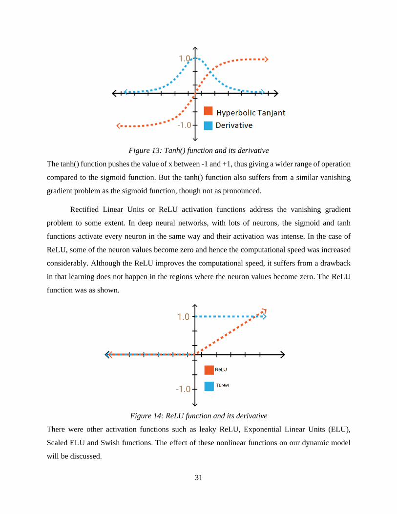
31
Figure 13: Tanh() function and its derivative
The tanh() function pushes the value of x between -1 and +1, thus giving a wider range of operation
compared to the sigmoid function. But the tanh() function also suffers from a similar vanishing
gradient problem as the sigmoid function, though not as pronounced.
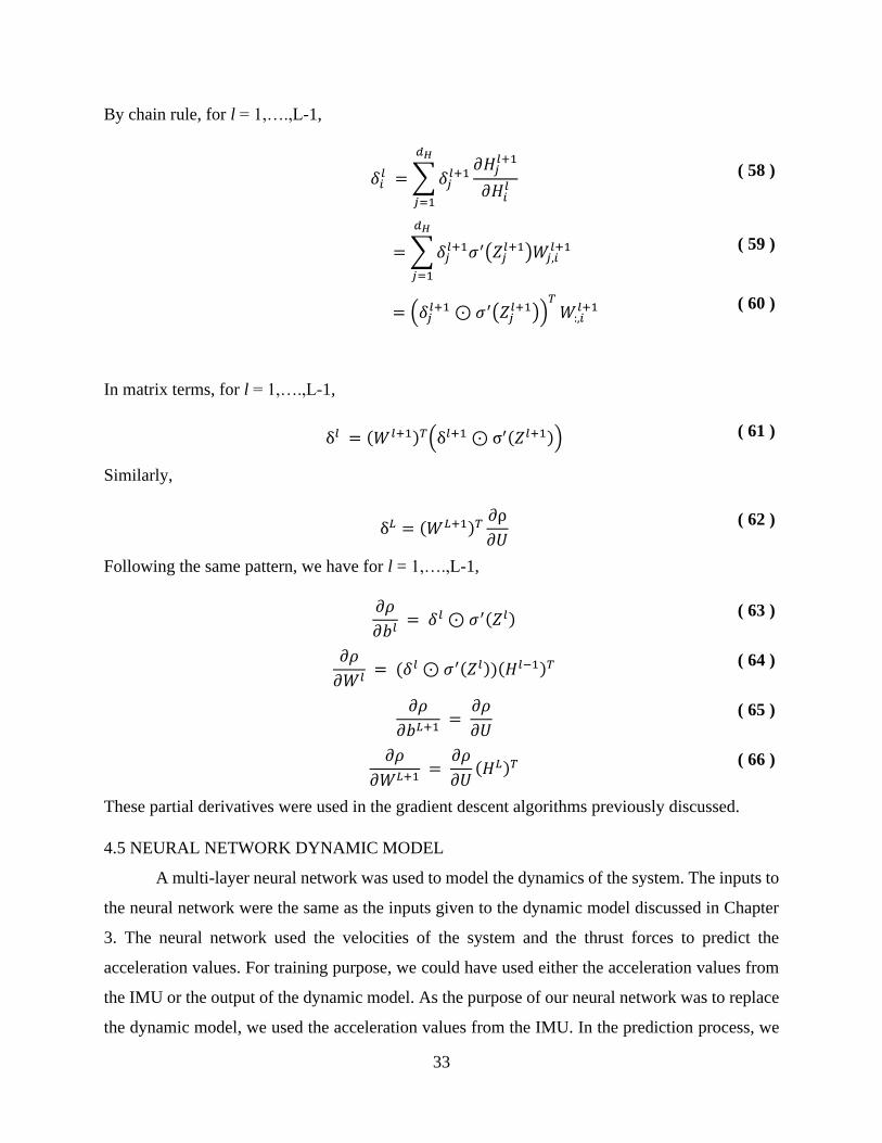
Rectified Linear Units or ReLU activation functions address the vanishing gradient
problem to some extent. In deep neural networks, with lots of neurons, the sigmoid and tanh
functions activate every neuron in the same way and their activation was intense. In the case of
ReLU, some of the neuron values become zero and hence the computational speed was increased
considerably. Although the ReLU improves the computational speed, it suffers from a drawback
in that learning does not happen in the regions where the neuron values become zero. The ReLU
function was as shown.
Figure 14: ReLU function and its derivative
There were other activation functions such as leaky ReLU, Exponential Linear Units (ELU),
Scaled ELU and Swish functions. The effect of these nonlinear functions on our dynamic model
will be discussed.

32
4.3 GRADIENT DESCENT
Neural networks estimate a statistical model for the relationship between an input X and
an output Y. Assume there is dataset (X, Y ) ϵ ℝ𝑑 x Y and a statistical model, f(x,θ) : ℝ𝑑 → ℝ𝐾.
θ ϵ Θ are the parameters in the model and must be estimated. We wish to find a model f(x,θ) such
that f(X,θ) is an accurate prediction for Y. We define our objective function as,
ℒ(θ) = 𝐸𝑋,𝑌[ρ(𝑓(𝑋; θ), 𝑌)] ( 53 )
θ is the set of parameters which minimizes the objective function.
θ = arg minθ′ ϵ Θ
ℒ(θ′) ( 54 )
The objective function can be minimized using gradient descent, the most popular choice for
training neural networks to obtain parameters θ. The gradient descent method is as shown below.
θ(𝑙+1) = θ(𝑙) − 𝛼(𝑙) ▽𝜃 (ℒ(θ(l))) ( 55 )
Here, ▽ is the gradient of the objective function in the steepest direction. The following gradient
descent algorithms were popularly used.
• Stochastic gradient descent [21]
• RMSprop [23]
• ADAM [24]
• AdaGrad [22]
4.4 BACK PROPAGATION
The gradient descent algorithms require the calculation of the gradients of ρ with respect
to the parameter set θ. For a multi-layer neural network mentioned previously, the parameter set
was as follows
θ = { 𝑊1, . . . . ,𝑊𝐿 , 𝑏1, . . . . , 𝑏𝐿 } ( 56 )
Let ρ ∶= ρ(𝑓(𝑋; θ), 𝑌). We define,
δ𝑙 ≔∂ρ
∂𝐻𝑙
( 57 )
33
By chain rule, for l = 1,….,L-1,
𝛿𝑖𝑙 = ∑𝛿𝑗
𝑙+1𝜕𝐻𝑗
𝑙+1
𝜕𝐻𝑖𝑙
𝑑𝐻
𝑗=1
( 58 )
= ∑𝛿𝑗𝑙+1𝜎′(𝑍𝑗
𝑙+1)𝑊𝑗,𝑖𝑙+1
𝑑𝐻
𝑗=1
( 59 )
= (𝛿𝑗𝑙+1 ⊙ 𝜎′(𝑍𝑗
𝑙+1))𝑇𝑊:,𝑖
𝑙+1 ( 60 )
In matrix terms, for l = 1,….,L-1,
δ𝑙 = (𝑊𝑙+1)𝑇(δ𝑙+1 ⊙ σ′(𝑍𝑙+1)) ( 61 )
Similarly,
δ𝐿 = (𝑊𝐿+1)𝑇∂ρ
∂𝑈
( 62 )
Following the same pattern, we have for l = 1,….,L-1,
𝜕𝜌
𝜕𝑏𝑙 = 𝛿𝑙 ⊙ 𝜎′(𝑍𝑙)
( 63 )
𝜕𝜌
𝜕𝑊𝑙 = (𝛿𝑙 ⊙ 𝜎′(𝑍𝑙))(𝐻𝑙−1)𝑇
( 64 )
𝜕𝜌
𝜕𝑏𝐿+1 =
𝜕𝜌
𝜕𝑈
( 65 )
𝜕𝜌
𝜕𝑊𝐿+1 =
𝜕𝜌
𝜕𝑈(𝐻𝐿)𝑇
( 66 )
These partial derivatives were used in the gradient descent algorithms previously discussed.
4.5 NEURAL NETWORK DYNAMIC MODEL
A multi-layer neural network was used to model the dynamics of the system. The inputs to
the neural network were the same as the inputs given to the dynamic model discussed in Chapter
3. The neural network used the velocities of the system and the thrust forces to predict the
acceleration values. For training purpose, we could have used either the acceleration values from
the IMU or the output of the dynamic model. As the purpose of our neural network was to replace
the dynamic model, we used the acceleration values from the IMU. In the prediction process, we
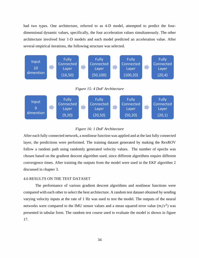
34
had two types. One architecture, referred to as 4-D model, attempted to predict the four-
dimensional dynamic values, specifically, the four acceleration values simultaneously. The other
architecture involved four 1-D models and each model predicted an acceleration value. After
several empirical iterations, the following structure was selected.
Figure 15: 4 DoF Architecture
Figure 16: 1 DoF Architecture
After each fully connected network, a nonlinear function was applied and at the last fully connected
layer, the predictions were performed. The training dataset generated by making the RexROV
follow a random path using randomly generated velocity values. The number of epochs was
chosen based on the gradient descent algorithm used, since different algorithms require different
convergence times. After training the outputs from the model were used in the EKF algorithm 2
discussed in chapter 3.
4.6 RESULTS ON THE TEST DATASET
The performance of various gradient descent algorithms and nonlinear functions were
compared with each other to select the best architecture. A random test dataset obtained by sending
varying velocity inputs at the rate of 1 Hz was used to test the model. The outputs of the neural
networks were compared to the IMU sensor values and a mean squared error value (𝑚/𝑠2) was
presented in tabular form. The random test course used to evaluate the model is shown in figure
17.
Input
10 dimention
Fully Connected
Layer
(16,50)
Fully Connected
Layer
(50,100)
Fully Connected
Layer
(100,20)
Fully Connected
Layer
(20,4)
Input
9 dimention
Fully Connected
Layer
(9,20)
Fully Connected
Layer
(20,50)
Fully Connected
Layer
(50,20)
Fully Connected
Layer
(20,1)
35
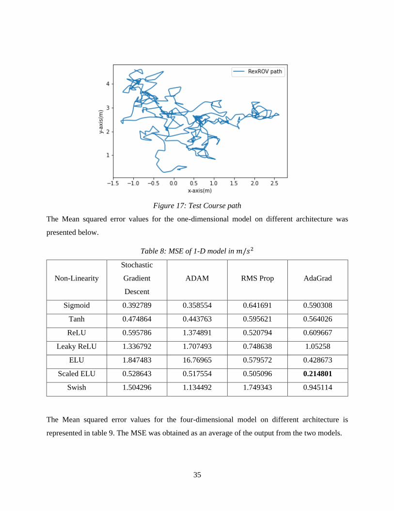
Figure 17: Test Course path
The Mean squared error values for the one-dimensional model on different architecture was
presented below.
Table 8: MSE of 1-D model in 𝑚/𝑠2
Non-Linearity
Stochastic
Gradient
Descent
ADAM RMS Prop AdaGrad
Sigmoid 0.392789 0.358554 0.641691 0.590308
Tanh 0.474864 0.443763 0.595621 0.564026
ReLU 0.595786 1.374891 0.520794 0.609667
Leaky ReLU 1.336792 1.707493 0.748638 1.05258
ELU 1.847483 16.76965 0.579572 0.428673
Scaled ELU 0.528643 0.517554 0.505096 0.214801
Swish 1.504296 1.134492 1.749343 0.945114
The Mean squared error values for the four-dimensional model on different architecture is
represented in table 9. The MSE was obtained as an average of the output from the two models.
36
Table 9: MSE of 4-D model output in 𝑚/𝑠2
Non-Linearity
Stochastic
Gradient
Descent
ADAM RMS Prop AdaGrad
Sigmoid 0.344719 0.385645 0.594746 0.590196
Tanh 0.467479 0.398121 0.640974 0.589978
ReLU 0.520794 1.607941 0.517014 0.344869
Leaky ReLU 1.739374 5.101167 0.509121 0.494125
ELU 1.67696 1.118611 0.480766 0.238511
Scaled ELU 0.564937 1.209875 0.283453 0.211873
Swish 1.515001 2.00879 0.548072 0.50399
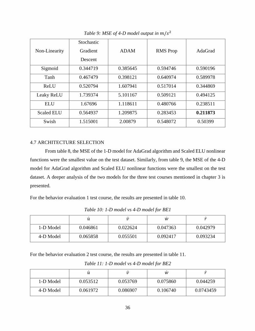
4.7 ARCHITECTURE SELECTION
From table 8, the MSE of the 1-D model for AdaGrad algorithm and Scaled ELU nonlinear
functions were the smallest value on the test dataset. Similarly, from table 9, the MSE of the 4-D
model for AdaGrad algorithm and Scaled ELU nonlinear functions were the smallest on the test
dataset. A deeper analysis of the two models for the three test courses mentioned in chapter 3 is
presented.
For the behavior evaluation 1 test course, the results are presented in table 10.
Table 10: 1-D model vs 4-D model for BE1
�� �� �� ��
1-D Model 0.046861 0.022624 0.047363 0.042979
4-D Model 0.065858 0.055501 0.092417 0.093234
For the behavior evaluation 2 test course, the results are presented in table 11.
Table 11: 1-D model vs 4-D model for BE2
�� �� �� ��
1-D Model 0.053512 0.053769 0.075860 0.044259
4-D Model 0.061972 0.086907 0.106740 0.0743459
37
For the behavior evaluation 3 test course, the results are presented in table 12.
Table 12: 1-D model vs 4-D model for BE3
�� �� �� ��
1-D Model 0.051806 0.030311 0.060022 0.047931
4-D Model 0.058105 0.052425 0.078260 0.057432
A deeper analysis demonstrated that for the MSE for 1-D model was better than the 4-D model.
We proceeded with the outputs from the 1-D model for our EKF algorithm.
4.8 NEURAL NETWORK MODEL VS DYNAMIC MODEL
The neural network architecture outputs were compared to the dynamic model outputs. The
results for the three behavior evaluation test courses were presented in figures 16 to 18.
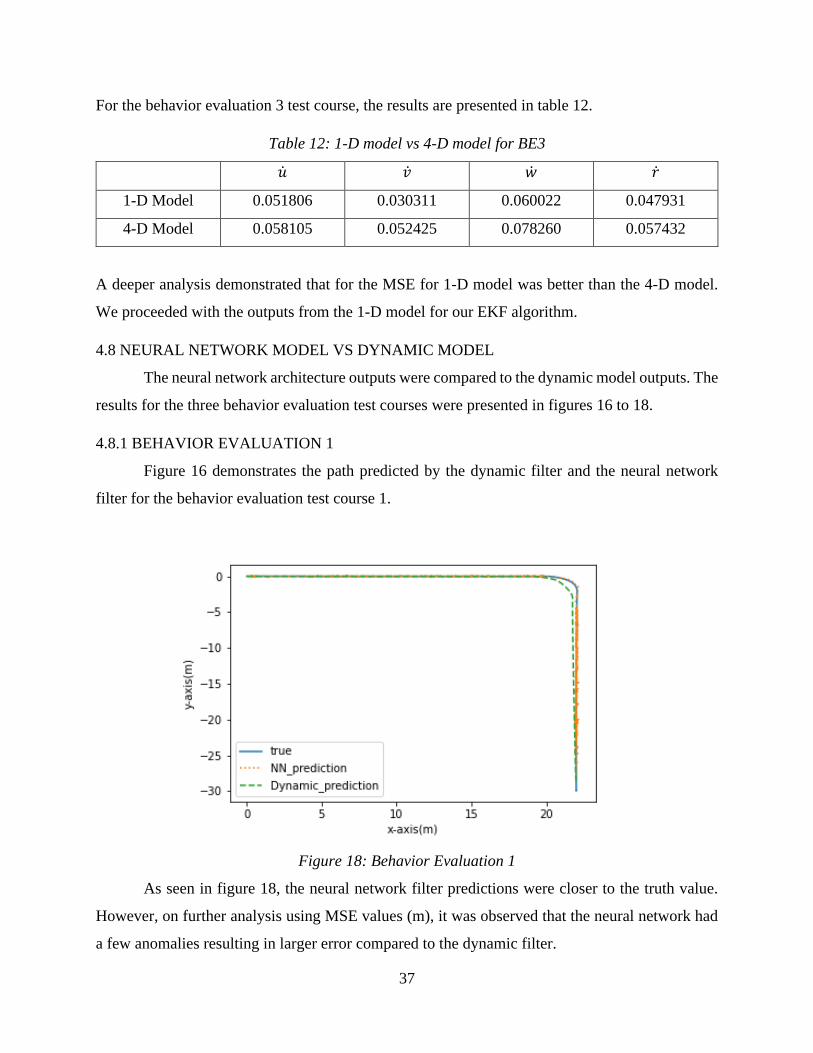
4.8.1 BEHAVIOR EVALUATION 1
Figure 16 demonstrates the path predicted by the dynamic filter and the neural network
filter for the behavior evaluation test course 1.
Figure 18: Behavior Evaluation 1
As seen in figure 18, the neural network filter predictions were closer to the truth value.
However, on further analysis using MSE values (m), it was observed that the neural network had
a few anomalies resulting in larger error compared to the dynamic filter.
38
Table 13: Results of Behavior Evaluation 1
Error (m) Dynamic Filter Neural Network Filter
Total 0.7572 1.5414
X-Kalman 0.5712 0.4148
Y-Kalman 0.4971 1.4846
From table 13, the total error of the dynamic filter was less than the neural network filter.
The neural network needs to be improvement in order to make better predictions for the Y-Kalman
values. In order to make further assessment of the filters, they were tested on the behavior
evaluation 2 test course.
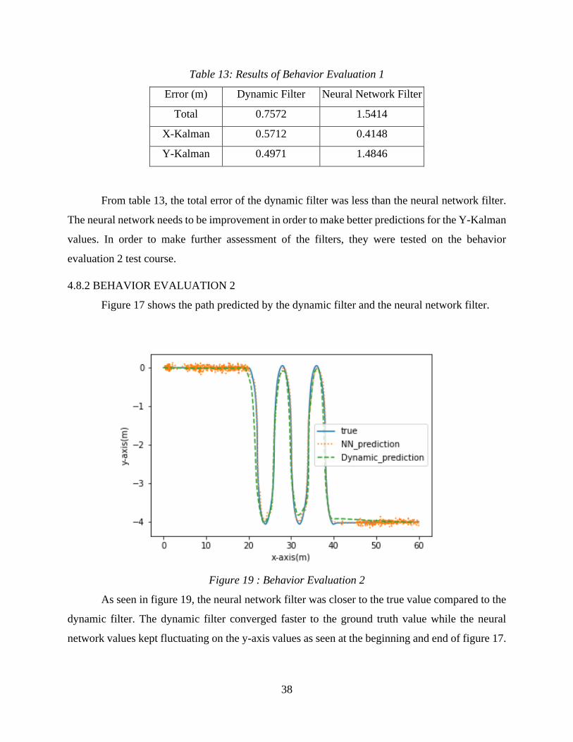
4.8.2 BEHAVIOR EVALUATION 2
Figure 17 shows the path predicted by the dynamic filter and the neural network filter.
Figure 19 : Behavior Evaluation 2
As seen in figure 19, the neural network filter was closer to the true value compared to the
dynamic filter. The dynamic filter converged faster to the ground truth value while the neural
network values kept fluctuating on the y-axis values as seen at the beginning and end of figure 17.
39
This further supports our conclusion from table 14 that the neural network should be improved to
make better predictions on the y-axis.
Table 14 : Results of Behavior Evaluation 2
Error (m) Dynamic Filter Neural Network Filter
Total 0.6697 0.6254
X-Kalman 0.3419 0.2391
Y-Kalman 0.5759 0.5779
From table 14, the mean error of the neural network filter was almost equal to the dynamic
filter. Both filters can handle the simultaneous changes in the x-axis and y-axis.
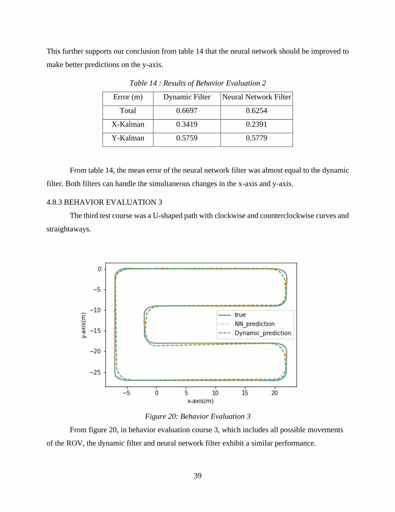
4.8.3 BEHAVIOR EVALUATION 3
The third test course was a U-shaped path with clockwise and counterclockwise curves and
straightaways.
Figure 20: Behavior Evaluation 3
From figure 20, in behavior evaluation course 3, which includes all possible movements
of the ROV, the dynamic filter and neural network filter exhibit a similar performance.
40
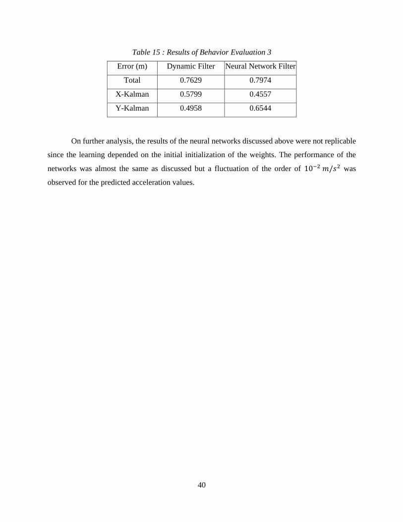
Table 15 : Results of Behavior Evaluation 3
Error (m) Dynamic Filter Neural Network Filter
Total 0.7629 0.7974
X-Kalman 0.5799 0.4557
Y-Kalman 0.4958 0.6544
On further analysis, the results of the neural networks discussed above were not replicable
since the learning depended on the initial initialization of the weights. The performance of the
networks was almost the same as discussed but a fluctuation of the order of 10−2 𝑚/𝑠2 was
observed for the predicted acceleration values.
41
CONCLUSION
A simplified 4 DoF dynamic model was derived for a RexROV and it was implemented on
an EKF. The outputs from the EKF were fed to a pure pursuit controller to control the RexROV in
the simulation. From the figures 8 to 10 and the tables 5 to 7, the dynamic Kalman filter predictions
were very close to the ground truth values. On comparison of the individual values predicted by
the dynamic filter and the kinematic filter with the actual position of RexROV, the dynamic filter
was more stable and reliable than the kinematic filter.
Since the dynamic model required the use of many coefficients, a neural network-based
approach was used to model the dynamics of the underwater vehicle. Several iterations, involving
four gradient descent algorithms and seven nonlinear activation functions, were performed to
choose the best architecture for the neural network. It was found that AdaGrad gradient descent
algorithm when used in combination with Scaled ELU activation function gave better results that
the other combinations. A comparison study was conducted on the three behavior test courses to
choose between the four 1-D models and 4-D model. It was found that the four 1-D models were
able to predict the acceleration values much more accurately than a single 4-D model. The
networks were trained to the maximum level without overfitting. The acceleration in y-axis(v) and
the acceleration in x-axis (u) were predicted to an accuracy of 0.05 𝑚/𝑠2 on a random test course.
The 1-D neural network models were used as an input to the EKF algorithm and the results
were compared to the dynamic filter. Both the neural-network and dynamic model were
implemented as a post-processing tool to maintain uniformity. The accuracy of the neural network
model was lower for the y coordinates on behavior evaluation test course 1. On further analysis, it
was found that the network was able to make better prediction on behavior evaluation test courses
2 and 3. The neural network was able to sufficiently replicate the dynamics of the vehicle although
a few more regularization and tuning needed to be performed to improve the network.
The neural network model was implemented as a post-processing tool and needs to be
implemented in the simulation in real-time to verify the performance. The neural network codes
were written in Pytorch and the controller codes on UUVSim used Cplusplus. Integrating the
Pytorch and Cplusplus environment should be done before the neural network model can be run
in real-time in UUVSim. The results were based on movement only in the two primary axes, x and
y, similar to a ground vehicle. Further research is being conducted on the simultaneous triaxial
42
movement to make the controller universal. It was expected that the movement on the z-axis should
not affect the performance of the dynamic Kalman filter and neural network filter.
Currently, the model uses GPS data to correct position estimation. However, research has
indicated that the strength of the electromagnetic waves for the GPS signal reduces significantly
underwater [27]. Methods such as station keeping, SONARSLAM and vision systems were
currently being explored as an alternative for position estimation. The results presented in this
thesis were obtained at a constant wave velocity. The wave velocity can be used as an input to the
neural network to better model the dynamics. The predictions were conducted at a frequency of
10Hz and the dynamic filter worked on the simulation without any performance issues. However,
the filters need to be implemented in real-time hardware to assess the actual computational
performance.
Another field of interest for the AUVSL group is prediction of the position of the vehicle
directly without the use of filters. Recurrent Neural Network algorithms such as LSTM can be
used to serve this purpose. One way to improve the Kalman filter predictions was to model the Q
and R matrix accurately. Generative Adversarial Nets (GANs) can be used to improve the accuracy
for Q and R. However, the GANs were limited by the availability of ground truth data for training.
The neural network modelling techniques discussed here were also applicable to the ground
vehicle which is currently explored by other members of AUVSL group. Alternative controller
techniques, such as sliding mode controller, were being researched to improve the performance of
the model.
43
REFERENCES
[1] Stillman, D. Oceans : The Great Unknown. Ed. by National Aeronautics and Space
Administration. 2009. url: https://www.nasa.gov/audience/forstudents/5-8/features/oceans-
the-great-unknown-58.html (visited on 06/29/2019).
[2] Manhaes, M.M.M.,et al.“UUV Simulator: A Gazebo-based package for underwater
intervention and multi-robot simulation”. In : OCEANS 2016 MTS/IEEE
Monterey.IEEE,Sept.2016.doi:10.1109/oceans.2016.7761080.
[3] Kermorgant, O., “A Dynamic Simulator for Underwater Vehicle-Manipulators”. In: vol. 8810.
Oct. 2014.doi:10.1007/978-3-319-11900-7_3.
[4] Kalman, R.E., “A New Approach to Linear Filtering and Pre-diction Problems”. In :
Transactions of the ASME–Journal of Basic Engineering 82.Series D (1960), pp. 35–45.
[5] Julier, S. J. and Uhlmann, J. K. "Unscented filtering and nonlinear estimation," in Proceedings
of the IEEE, vol. 92, no. 3, pp. 401-422, March 2004, doi: 10.1109/JPROC.2003.823141.
[6] Romagos, D., Ridao, P., and Neira, J. Underwater SLAM for Structured Environments Using
an Imaging Sonar. Vol.65. Jan.2010. isbn:978-3-642-14039-6.doi:10.1007/978-3-642-14040-
2.
[7] Hascaryo, R. W., 2019. “Reduced order extended Kalman filter incorporating dynamics of an
autonomous underwater vehicle for motion prediction”, Master’s Thesis, Department of
Aerospace Engineering, University of Illinois at Urbana Champaign, USA.
[8] Berg, V., 2012. “Development and commissioning of adp system for rov sf 30k”, Master’s
thesis, Department of Engineering Cybernetics, Norwegian University of Science and
Technology, Trondheim, Norway, 2012.
[9] Adam, A., and Erik, E., 2016. “Model-based design, development, and control of an
underwater vehicle”, Master’s thesis, Department of Electrical Engineering, Linkoping
University, Linkoping, Sweden, 2016.
[10] Govinda, L., Tomas, S., Bandala, M., Nava Balanzar, L., Hernandez-Alvarado, R., and
Antonio, J., 2014.“Modelling, design and robust control of a remotely operated
underwater vehicle”. International Journal of Advanced Robotic Systems,11, 01, p. 1.
[11] Norris, W.R., and Patterson, A.E., 2019. “System-level testing and evaluation plan for
field robots: A tutorial with test course layouts”. Robotics, 8(4).

44
[12] Abadi, M., Agarwal, A., Barham, P., et al TensorFlow: Large-scale machine learning on
heterogeneous systems, 2015. Software available from tensorflow.org.
[13] Paszke, A., Gross, S., Massa, F., Lerer, A., Bradbury, J., Chanan, G., … Chintala, S. (2019).
PyTorch: An Imperative Style, High-Performance Deep Learning Library. In H. Wallach, H.
Larochelle, A. Beygelzimer, F. d extquotesingle Alch'e-Buc, E. Fox, & R. Garnett
(Eds.), Advances in Neural Information Processing Systems 32 (pp. 8024–8035). Curran
Associates Inc. Retrieved from http://papers.neurips.cc/paper/9015-pytorch-an-imperative-
style-high-performance-deep-learning-library.pdf.
[14] Fossen, T. I., Handbook of Marine Craft Hydrodynamics and Motion Control, 1st Ed., Wiley,
Chichester, United Kingdom, 2011, Chapters 1-7, 12.
[15] Fossen, T. I., “Nonlinear Modelling and Control of Underwater Vehicle”, PhD dissertation,
Department of Engineering Cybernetics, Norwegian University of Science and Technology,
Trondheim, Norway, 1991.
[16] Rosa, R., Zaffari, G., Evald, P., Drews-Jr, P., Botelho, S. (2017). “Towards Comparison of
Kalman Filter Methods for Localisation in Underwater Environments”, 10.1109/SBR-LARS-
R.2017.8215339.
[17] Manhaes, M., Scherer, S. A., Douat, L. R., Voss, M. and Rauschenbach, T. "Use of simulation-
based performance metrics on the evaluation of dynamic positioning controllers", OCEANS
2017 - Aberdeen, Aberdeen, 2017, pp. 1-8,doi: 10.1109/OCEANSE.2017.8084658.
[18] Kleene, S.C. (1956). "Representation of Events in Nerve Nets and Finite Automata". Annals
of Mathematics Studies (34). Princeton University Press. pp. 3–41. Retrieved 17 June 2017
[19] Schmidhuber, J. “Deep Learning in Neural Networks: An Overview”.In : CoRRabs/1404.7828
(2014). arXiv:1404.7828. url : http://arxiv.org/abs/1404.7828.
[20] Yiu, T., “Understanding Neural Networks. Ed. by Towards Datascience”, 2019. url :
https://towardsdatascience.com/understanding-neural-networks-19020b758230 (visited on
06/29/2019).
[21] Goodfellow, I., Bengio, Y., and Courville, A. Deep Learning. MIT Press, 2016.
[22] Duchi, J., Hazan, E., and Singer, Y., 2011. “Adaptive Subgradient Methods for Online
Learning and Stochastic Optimization”. J. Mach. Learn. Res., 12:2121–2159.
45
[23] Hinton, G. 2012. Neural Networks for Machine Learning - Lecture 6a - Overview of mini-
batch gradient descent.
[24] Kingma, D.P., and Ba, J. 2014. “Adam: A Method for Stochastic Optimization”. CoRR,
abs/1412.6980.
[25] Coulter, R. C., 1992. “Implementation of pure pursuit path tracking algorithm”. The Robotics
Institute, Carnegie Mellon University.
[26] Agudelo, J. G., 2015. “Contribution to the model and navigation control of an autonomous
underwater vehicle”, PhD thesis, PhD thesis, Departament d’Enginyeria Electronica,
Universitat Politecnica de Catalunya.
[27] Taraldsen, G., Reinen, T. A., and Berg, T., 2011. “The underwater gps problem”, In
OCEANS 2011 IEEE - Spain, pp. 1–8.