Neural Network Language Modeling - Wei Xu · Neural Network Language Modeling Many slides from...

Neural Network Language Modeling

Many slides from Marek Rei, Philipp Koehn and Noah Smith

Instructor: Wei Xu Ohio State University

CSE 5525

Course Project• Sign up your course project • In-class presentation on next Friday, 5 minute each

Language Modeling (Recap)•Goal:

- calculate the probability of a sentence

- calculate probability of a word in the sentence

N-gram Language Modeling (Recap)

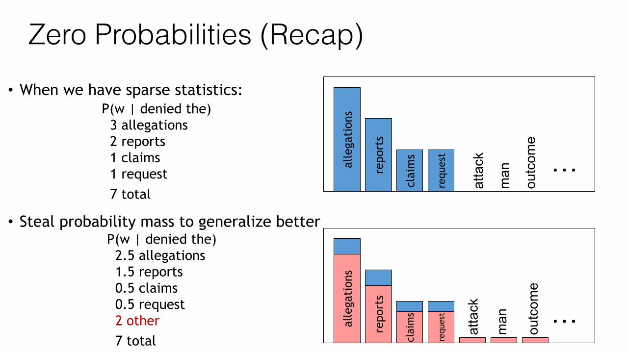
Zero Probabilities (Recap)• When we have sparse statistics:

• Steal probability mass to generalize better

P(w | denied the) 3 allegations 2 reports 1 claims 1 request 7 total

P(w | denied the) 2.5 allegations 1.5 reports 0.5 claims 0.5 request 2 other 7 total

alle

gati

ons

repo

rts

clai

ms

atta

ck

requ

est

man

outc

ome

…

alle

gati

ons

atta

ck

man

outc

ome

…alle

gati

ons

repo

rts

clai

ms

requ

est

•Backoff • Interpolation

•Kneser-Ney Smoothing

Smoothing (Recap)

Problems with N-grams• Problem 1: N-grams are sparse.

- There are V4 possible 4-grams. With V=10,000, that’s 1016 4-grams.

- We will only see a tiny fraction of them in our training data.

Problems with N-grams• Problem 2: Words are independent.

- It only map together identical words, but ignore similar or related words.

- If we have seen “yellow daffodil” in the data, we could use the intuition that “blue” is related to “yellow” to handle “blue daffodils”.

Vector Representation• Let’s represent words (or any objects) as vectors. • Let’s choose them, so that similar words have similar vectors.

One-hot Word Vectors• Each element represents the word.

One-hot Word Vectors• That’s a very large vector! • They tell us very little.

• Each element represents a property, and they are shared between the words.

Distributed Vectors (Representations)

• Groups similar words/objects together.

Distributed Vectors

Distributed Vectors• Use cosine similarity to calculate similarity between two words

Distributed Vectors• We can infer some information based only on the vector of the word.

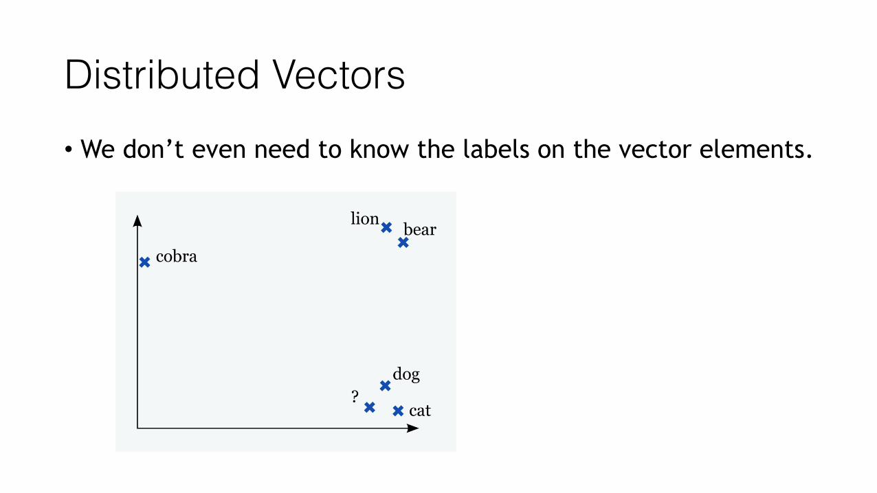
Distributed Vectors• We don’t even need to know the labels on the vector elements.

Distributed Vectors• The vectors are usually not 2 or 3-dimensional. More often

100-1000 dimensions.

Neural Network Language Models• Represent each word as a vector, and similar words with similar

vectors.

• Idea: • similar contexts have similar words • so we define a model that aims to predict between a word wt

and context words: P(wt|context) or P(context|wt) • Optimize the vectors together with the model, so we end up

with vectors that perform well for language modeling (aka representation learning)

Artificial Neuron

Perceptrons = Single-Layer Neural Networks !

Artificial Neuron

Neural Network• Many neurons connected together

Multi-Layer Feed-Forward Networks!

Neural Network• Usually, a neuron is shown as a single unit

Neural Network• Or a whole layer of neurons is represented as a block

Neuron Activation w/ Vectors

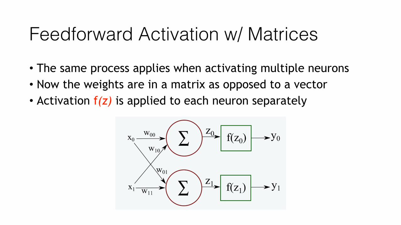
Feedforward Activation w/ Matrices • The same process applies when activating multiple neurons • Now the weights are in a matrix as opposed to a vector • Activation f(z) is applied to each neuron separately

Feedforward Activation w/ Matrices

Neural Network

Feedforward Activation

1) Take vector from the previous layer 2) Multiply it with the weight matrix 3) Apply the activation function 4) Repeat

Feedforward Activation

Exercise

Input Layer

1

1.0

0.0

1

4.5

-5.2

-2.0-4.6-1.5

3.72.9

3.7

2.9

Hidden Layer Computation.90

.17

1

1.0

0.0

1

4.5

-5.2

-2.0-4.6-1.5

3.72.9

3.7

2.9

Output Layer Computation

.90

.17

1

.76

1.0

0.0

1

4.5

-5.2

-2.0-4.6-1.5

3.72.9

3.7

2.9

Error 18Error

.90

.17

1

.76

1.0

0.0

1

4.5

-5.2

-2.0-4.6-1.5

3.72.9

3.7

2.9

• Computed output: y = .76

• Correct output: t = 1.0

) How do we adjust the weights?

Philipp Koehn Machine Translation: Introduction to Neural Networks 12 April 2016

Back-propagation Training19Key Concepts

• Gradient descent

– error is a function of the weights– we want to reduce the error– gradient descent: move towards the error minimum– compute gradient ! get direction to the error minimum– adjust weights towards direction of lower error

• Back-propagation

– first adjust last set of weights– propagate error back to each previous layer– adjust their weights


Final Layer Update21Final Layer Update

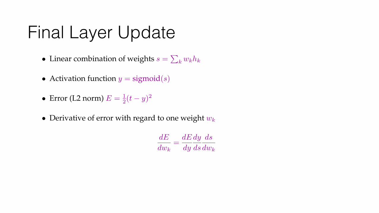
• Linear combination of weights s =P

k

w

k

h

k

• Activation function y = sigmoid(s)

• Error (L2 norm) E = 12(t� y)2

• Derivative of error with regard to one weight wk

dE

dw

k

=dE

dy

dy

ds

ds

dw

k


Final Layer Update (1)22Final Layer Update (1)


k

w

k

h

k




dE

dw

k

=dE

dy

dy

ds

ds

dw

k

• Error E is defined with respect to y

dE

dy

=d

dy

1

2(t� y)2 = �(t� y)




k

w

k

h

k




dE

dw

k

=dE

dy

dy

ds

ds

dw

k

• y with respect to x is sigmoid(s)

dy

ds

=d sigmoid(s)

ds

= sigmoid(s)(1� sigmoid(s)) = y(1� y)




k

w

k

h

k




dE

dw

k

=dE

dy

dy

ds

ds

dw

k

• x is weighted linear combination of hidden node values hk

ds

dw

k

=d

dw

k

X

k

w

k

h

k

= h

k


Putting it Together 25Putting it All Together


dE

dw

k

=dE

dy

dy

ds

ds

dw

k

= �(t� y) y(1� y) h

k

– error– derivative of sigmoid: y0

• Weight adjustment will be scaled by a fixed learning rate µ

�w

k

= µ (t� y) y0 hk


Multiple Output Nodes 26Multiple Output Nodes

• Our example only had one output node

• Typically neural networks have multiple output nodes

• Error is computed over all j output nodes

E =X

j

1

2(t

j

� y

j

)2

• Weights k ! j are adjusted according to the node they point to

�w

j k

= µ(tj

� y

j

) y0j

h

k


Hidden Layer Update27Hidden Layer Update

• In a hidden layer, we do not have a target output value

• But we can compute how much each node contributed to downstream error

• Definition of error term of each node

�

j

= (tj

� y

j

) y0j

• Back-propagate the error term(why this way? there is math to back it up...)

�

i

=⇣X

j

w

j i

�

j

⌘y

0i

• Universal update formula�w

j k

= µ �

j

h

k


Final Layer Update (example) 28Our Example

.90

.17

1

.76

1.0

0.0

1

4.5

-5.2

-2.0-4.6-1.5

3.72.9

3.7

2.9

A

B

C

D

E

F

G



• Final layer weight updates (learning rate µ = 10)– �

G

= (t� y) y0 = (1� .76) 0.181 = .0434

– �w

GD

= µ �

G

h

D

= 10⇥ .0434⇥ .90 = .391

– �w

GE

= µ �

G

h

E

= 10⇥ .0434⇥ .17 = .074

– �w

GF

= µ �

G

h

F

= 10⇥ .0434⇥ 1 = .434


Final Layer Update (example) 29Our Example

.90

.17

1

.76

1.0

0.0

1

4.5

-5.2

-2.0-4.6-1.5

3.72.9

3.7

2.9

A

B

C

D

E

F

G

4.891 —

-5.126 ——

-1.566 ——



• Final layer weight updates (learning rate µ = 10)– �

G

= (t� y) y0 = (1� .76) 0.181 = .0434

– �w

GD

= µ �

G

h

D

= 10⇥ .0434⇥ .90 = .391

– �w

GE

= µ �

G

h

E

= 10⇥ .0434⇥ .17 = .074

– �w

GF

= µ �

G

h

F

= 10⇥ .0434⇥ 1 = .434


Hidden Layer Update (example) 30Hidden Layer Updates

.90

.17

1

.76

1.0

0.0

1

4.5

-5.2

-2.0-4.6-1.5

3.72.9

3.7

2.9

A

B

C

D

E

F

G

4.891 —

-5.126 ——

-1.566 ——

• Hidden node D

– �

D

=⇣P

j

w

j i

�

j

⌘y

0D

= w

GD

�

G

y

0D

= 4.5⇥ .0434⇥ .0898 = .0175

– �w

DA

= µ �

D

h

A

= 10⇥ .0175⇥ 1.0 = .175– �w

DB

= µ �

D

h

B

= 10⇥ .0175⇥ 0.0 = 0– �w

DC

= µ �

D

h

C

= 10⇥ .0175⇥ 1 = .175

• Hidden node E

– �

E

=⇣P

j

w

j i

�

j

⌘y

0E

= w

GE

�

G

y

0E

= �5.2⇥ .0434⇥ 0.2055 = �.0464

– �w

EA

= µ �

E

h

A

= 10⇥�.0464⇥ 1.0 = �.464– etc.


Initialization of Weights32Initialization of Weights

• Weights are initialized randomlye.g., uniformly from interval [�0.01, 0.01]

• Glorot and Bengio (2010) suggest

– for shallow neural networks⇥� 1p

n

,

1pn

⇤

n is the size of the previous layer

– for deep neural networks

⇥�

p6

pn

j

+ n

j+1,

p6

pn

j

+ n

j+1

⇤

n

j

is the size of the previous layer, nj

size of next layer


Neural Networks for Classification33Neural Networks for Classification

• Predict class: one output node per class

• Training data output: ”One-hot vector”, e.g., ~y = (0, 0, 1)T

• Prediction– predicted class is output node y

i

with highest value– obtain posterior probability distribution by soft-max

softmax(yi

) =e

y

i

Pj

e

y

j


Feedforward Neural Network Language Model• Input: vector representations of previous words E(wi-3) E(wi-2) E (wi-1) • Output: the conditional probability of wj being the next word

• We can also think of the input as a concatenation of the context vectors • The hidden layer h is calculated as in previous examples

How do we calculate ?

Feedforward Neural Network Language Model

• Our output vector o has an element for each possible word wj

• We take a softmax over that vector

How do we calculate ?


• Our output vector o has an element for each possible word wj

• We take a softmax over that vector


1) Multiple input vectors with weights

2) Apply the activation function

Bengio et al. (2003)


3) Multiply hidden vector with output weights

4) Apply softmax to the output vector

Now the j-th element in the output vector oj contains the probability of wj being the next word.


tanh

softmax


Like a log-linear language model with two kinds of features:

1) concatenation of context-word embedding vectors

2) tanh-affine transformation of the above



tanh

softmax

one hot vectors

tanh

softmax

one hot vectors

Visualization

Mu,T

b, A

tanh

softmaxW

14 / 57



Neural Network: DefinitionsWarning: there is no widely accepted standard notation!

A feedforward neural network n⌫ is defined by:I A function family that maps parameter values to functions of

the form n : Rdin

! Rdout ; typically:

I Non-linearI Di↵erentiable with respect to its inputsI “Assembled” through a series of a�ne transformations and

non-linearities, composed togetherI Symbolic/discrete inputs handled through lookups.

I Parameter values ⌫I Typically a collection of scalars, vectors, and matricesI We often assume they are linearized into RD

3 / 57

A Couple of Useful FunctionsI

softmax : Rk! Rk

hx1

, x2

, . . . , xki 7!

*ex1

Pkj=1

exj,

ex2

Pkj=1

exj, . . . ,

exk

Pkj=1

exj

+

Itanh : R ! [�1, 1]

x 7!

ex � e�x

ex + e�x

Generalized to be elementwise, so that it maps Rk! [�1, 1]k.

I Others include: ReLUs, logistic sigmoids, PReLUs, . . .

4 / 57

Feedforward Neural Network Language Model(Bengio et al., 2003)

Define the n-gram probability as follows:

p(· | hh1

, . . . , hn�1

i) = n⌫�heh1 , . . . , ehn�1i

�=

softmax

0

@b

V

+

n�1X

j=1

ehj

V

>M

V ⇥ d

Ajd ⇥ V

+ W

V ⇥ H

tanh

0

@u

H

+

n�1X

j=1

e

>hjM Tj

d ⇥ H

1

A

1

A

where each ehj2 RV is a one-hot vector and H is the number of

“hidden units” in the neural network (a “hyperparameter”).

Parameters ⌫ include:

IM 2 RV⇥d, which are called “embeddings” (row vectors), onefor every word in V

I Feedforward NN parameters b 2 RV , A 2 R(n�1)⇥d⇥V ,W 2 RV⇥H , u 2 RH , T 2 R(n�1)⇥d⇥H

6 / 57

Visualization

Mu,T

b, A

tanh

softmaxW

14 / 57

Feedforward Neural Network Language Model(Bengio et al., 2003)

Define the n-gram probability as follows:

p(· | hh1

, . . . , hn�1

i) = n⌫�heh1 , . . . , ehn�1i

�=

softmax

0

@b

V

+

n�1X

j=1

ehj

V

>M

V ⇥ d

Ajd ⇥ V

+ W

V ⇥ H

tanh

0

@u

H

+

n�1X

j=1

e

>hjM Tj

d ⇥ H

1

A

1

A

where each ehj2 RV is a one-hot vector and H is the number of

“hidden units” in the neural network (a “hyperparameter”).

Parameters ⌫ include:

IM 2 RV⇥d, which are called “embeddings” (row vectors), onefor every word in V

I Feedforward NN parameters b 2 RV , A 2 R(n�1)⇥d⇥V ,W 2 RV⇥H , u 2 RH , T 2 R(n�1)⇥d⇥H

6 / 57

Breaking It Down

Look up each of the history words hj , 8j 2 {1, . . . , n� 1} in M;keep two copies.

ehj

V

>M

V ⇥ d

ehj

V

>M

V ⇥ d

7 / 57

Breaking It Down

Look up each of the history words hj , 8j 2 {1, . . . , n� 1} in M;keep two copies. Rename the embedding for hj as mhj

.

ehj

>M = mhj

ehj

>M = mhj

8 / 57

Visualization

Mu,T

b, A

tanh

softmaxW

14 / 57

Breaking It Down


ehj

V

>M

V ⇥ d

ehj

V

>M

V ⇥ d

7 / 57

Visualization

Mu,T

b, A

tanh

softmaxW

14 / 57

Breaking It Down

Apply an a�ne transformation to the second copy of thehistory-word embeddings (u, T)

mhj

u

H

+

n�1X

j=1

mhjTjd ⇥ H

9 / 57

Breaking It Down


ehj

V

>M

V ⇥ d

ehj

V

>M

V ⇥ d

7 / 57

Visualization

Mu,T

b, A

tanh

softmaxW

14 / 57

Breaking It Down

Apply an a�ne transformation to the second copy of thehistory-word embeddings (u, T) and a tanh nonlinearity.

mhj

tanh

0

@u +

n�1X

j=1

mhjTj

1

A

10 / 57

Breaking It Down

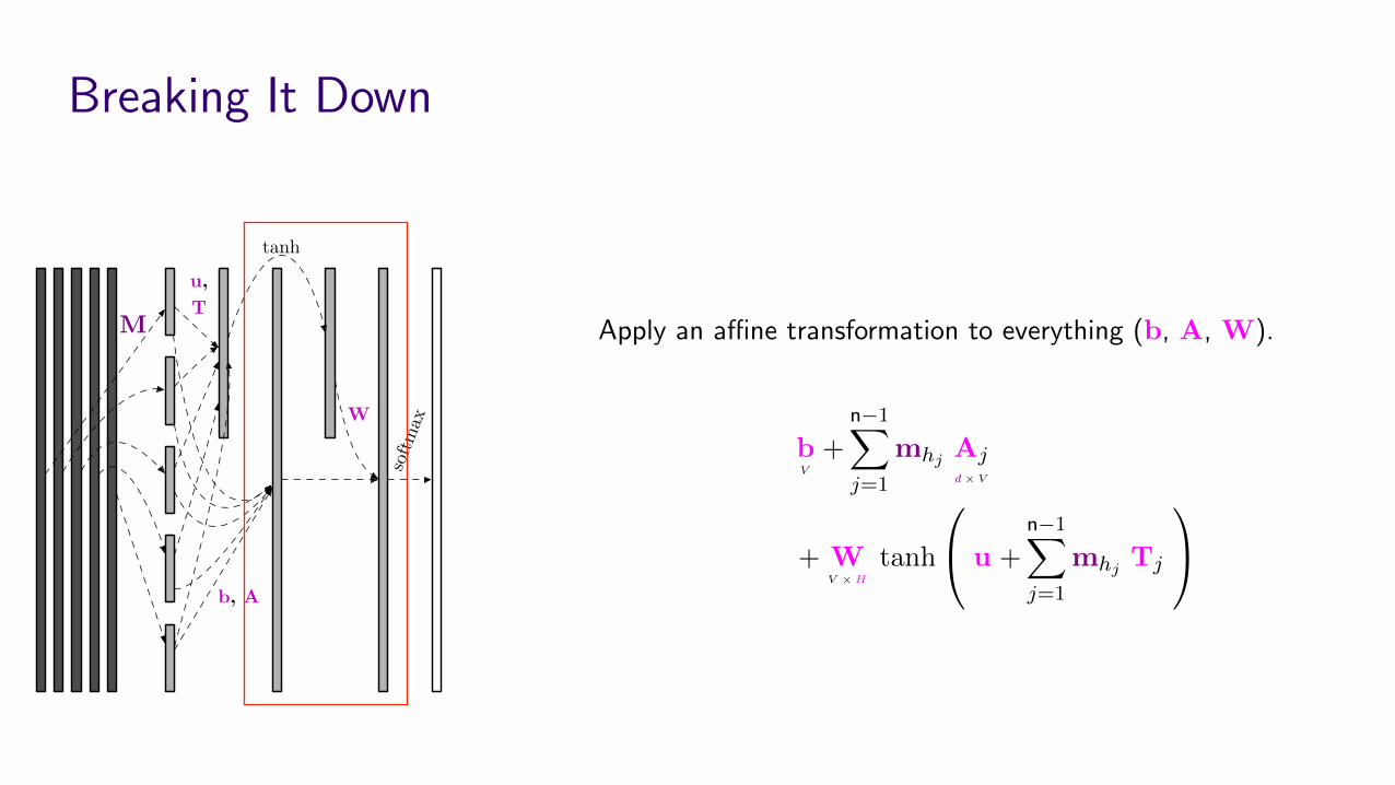
Apply an a�ne transformation to everything (b, A, W).

b

V

+

n�1X

j=1

mhjAjd ⇥ V

+ W

V ⇥ H

tanh

0

@u +

n�1X

j=1

mhjTj

1

A

11 / 57

Breaking It Down


ehj

V

>M

V ⇥ d

ehj

V

>M

V ⇥ d

7 / 57

Visualization

Mu,T

b, A

tanh

softmaxW

14 / 57

Breaking It Down


ehj

V

>M

V ⇥ d

ehj

V

>M

V ⇥ d

7 / 57

Visualization

Mu,T

b, A

tanh

softmaxW

14 / 57

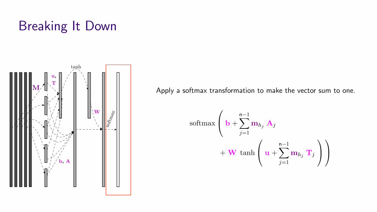
Breaking It Down

Apply a softmax transformation to make the vector sum to one.

softmax

0

@b +

n�1X

j=1

mhjAj

+ W tanh

0

@u +

n�1X

j=1

mhjTj

1

A

1

A

12 / 57

Breaking It Down


ehj

V

>M

V ⇥ d

ehj

V

>M

V ⇥ d

7 / 57

Visualization

Mu,T

b, A

tanh

softmaxW

14 / 57

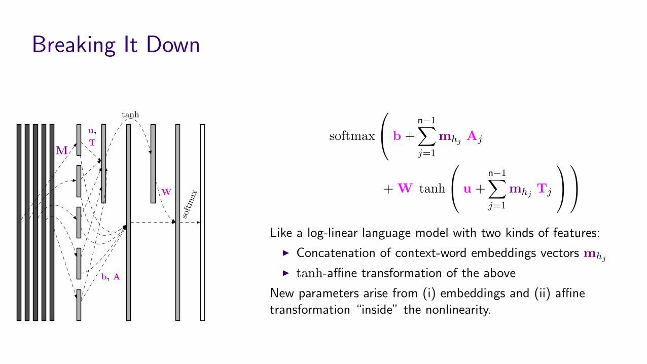
Breaking It Down

softmax

0

@b +

n�1X

j=1

mhjAj

+ W tanh

0

@u +

n�1X

j=1

mhjTj

1

A

1

A

Like a log-linear language model with two kinds of features:

I Concatenation of context-word embeddings vectors mhj

Itanh-a�ne transformation of the above

New parameters arise from (i) embeddings and (ii) a�netransformation “inside” the nonlinearity.

13 / 57

Number of Parameters

D = V d|{z}M

+ V|{z}b

+(n� 1)dV| {z }A

+ V H|{z}W

+ H|{z}u

+(n� 1)dH| {z }T

For Bengio et al. (2003):I V ⇡ 18000 (after OOV processing)I d 2 {30, 60}I H 2 {50, 100}I n� 1 = 5

So D = 461V + 30100 parameters, compared to O(V n) for

classical n-gram models.

I Forcing A = 0 eliminated 300V parameters and performed abit better, but was slower to converge.

I If we averaged mhjinstead of concatenating, we’d get to

221V + 6100 (this is a variant of “continuous bag of words,”Mikolov et al., 2013).

15 / 57


D = V d|{z}M

+ V|{z}b

+(n� 1)dV| {z }A

+ V H|{z}W

+ H|{z}u

+(n� 1)dH| {z }T







15 / 57

Visualization

Mu,T

b, A

tanh

softmaxW

14 / 57


D = V d|{z}M

+ V|{z}b

+(n� 1)dV| {z }A

+ V H|{z}W

+ H|{z}u

+(n� 1)dH| {z }T







15 / 57

Why does it work?

Neural Network Language Modeling - Wei Xu · Neural Network Language Modeling Many slides from...

Documents

Transcript of Neural Network Language Modeling - Wei Xu · Neural Network Language Modeling Many slides from...