Neural network detection of grinding burn from acoustic ...

International Journal of Machine Tools & Manufacture 41 (2001) 283–309

Neural network detection of grinding burn from acousticemission

Zhen Wanga, Peter Willetta,*, Paulo R. DeAguiarb, John Websterc

a Information & Computing Systems Group, Electrical and Systems Engineering Department, U-157, University ofConnecticut, Storrs, CT, 06268-2157, USA

b Universidade Estadual Paulista – Unesp, Departamento de Engenharia Eletrica, Av. Luiz Edmundo C. Coube, s/n,Vargem Limpa, Bauru, Sa˜o Paulo, Cep 17033-360, Brazil

c Unicorn International, Grinding Technology Centre, Tuffley Crescent, Gloucester GL1 5NG, UK

Received 7 March 2000; accepted 30 June 2000

Abstract

An artificial neural network (ANN) approach is proposed for the detection of workpiece “burn”, theundesirable change in metallurgical properties of the material produced by overly aggressive or otherwiseinappropriate grinding. The grinding acoustic emission (AE) signals for 52100 bearing steel were collectedand digested to extract feature vectors that appear to be suitable for ANN processing. Two feature vectorsare represented: one concerning band power, kurtosis and skew; and the other autoregressive (AR) coef-ficients. The result (burn or no-burn) of the signals was identified on the basis of hardness and profile testsafter grinding. The trained neural network works remarkably well for burn detection. Other signal-pro-cessing approaches are also discussed, and among them the constant false-alarm rate (CFAR) power lawand the mean-value deviance (MVD) prove useful. 2000 Elsevier Science Ltd. All rights reserved.

Keywords:Acoustic emission; Grinding; Burn detection; Neural network

1. Introduction

Acoustic emission (AE) is generally understood as the release of a vibrational wave emittedby a material reacting to applied stress. The acoustic emission generated during grinding andmachining processes has been proved to be related to the process state and to the surface conditionof the tool and workpiece [11,16]. AE technology has progressed significantly and has been widely

* Corresponding author. Tel.:+1-860-486-2195; fax:+1-860-486-5585.E-mail address:[email protected] (P. Willett).

0890-6955/01/$ - see front matter 2000 Elsevier Science Ltd. All rights reserved.PII: S0890-6955(00)00057-2

284 Z. Wang et al. / International Journal of Machine Tools & Manufacture 41 (2001) 283–309

investigated as a non-destructive testing method for monitoring grinding and machining processes,including wheel/work contact [16,9], surface integrity [26], metal cutting [10], tool wear [5], etc.Most formal research has relied on AE root-mean-square (RMS) power and statistics derivedtherefrom to determine the grinding condition and performance. Since the “averaging” nature ofRMS makes it insensitive to short-duration events (such as cracks) which may be of interest, herewe use instead the raw AE signals as collected by a high-frequency (2.56 MHz) analog-to-digital(A/D) converter.

Of particular interest to us here is the detection of superficial workpiece burn during the grindingprocess. When the energy in the wheel/workpiece contact area generates a temperature increase,this can lead to an increased tendency for adhesion of metal particles to the abrasive grains,thereby accelerating the rise in temperature. This causes burning of the workpiece. This is some-times observable visually by a bluish temper color, but more generally requires time-consumingchemical means for its after-the-fact determination. To increase the effectiveness of the grindingprocess and reduce the cost, reasonable in-process detection of burn is clearly of major interestin grinding operations. Prior successful application of AE in grinding, and the fact that the AEsignals are generated directly in the deformation zone of the grinding process and are thereforepresumably closely connected to the condition of the workpiece surface, make AE a promisingmeans to detect burn.

Previously [4,14] AE amplitude analysis was used, based on the observation that suddenchanges in the AE RMS power can be indicative of burn. In many cases, burn does not have alarge signature in the power level of the AE signal. Wheel-period correlation was introduced in[8], and could be used quite accurately to determine the rotational speed of the grinding wheel.The variation in wheel speed and the level of self-correlation of the AE signal between wheelrotations were used to indicate burn. It should be noted that these are methods relying on singlestatistics, and hence may be termedthresholdmethods. When AE is applied to burn detection ingrinding, the noise resulting from the normal grinding process complicates burn detection. It isdifficult to separate AE signals from normal grinding and from burn generation — especiallyas they can be emitted simultaneously from essentially the same physical location — with athreshold method.

We have applied a number of (thresholdable) statistics in this paper. One of these is statisticalanalysis based on the distribution moments of the AE signal. A popular one of these is the kurtosis[2,12], defined as a ratio of the fourth central moment to the square of the second central moment.The kurtosis and skewness statistics have attracted considerable interest [18], since it is supposedthat they are sensitive to a process change, such as metal fracture, the occurrence of tool failureor burn. The skewness (normalized central third moment) measures the symmetry of a probabilitydistribution, while the kurtosis is a measure both of the sharpness of the distribution’s peak andthe probability of outlying (unexpectedly large) samples. Both time- and frequency-domain kur-tosis analyses have been explored using real data; it is apparent that some more sophisticatedapproach is necessary.

Despite the name, a neural network (NN) is basically an adaptive non-linear functional approx-imator. The non-linear mapping implicit to the NN is determined by adjustableparameters, withthese trained from a data set. There are two broad classes of NN. The most easily recognized isthe multi-layer perceptron (MLP), whose feed-forward structure and sigmoidal “neurons” wereoriginally supposed to mimic those of the brain. The other structure is that of the radial basis

285Z. Wang et al. / International Journal of Machine Tools & Manufacture 41 (2001) 283–309

function (RBF) network, which can be thought of as a functional approximator using (usually)Gaussian-shaped kernels. For the present discussion, the important characteristics of both NNsare their ability to recognize and realize general functions as suggested by training data, and theircorrelative ability to explain their outputs by groups of input data, taken jointly. Thus it is naturalto consider an NN when a threshold method does not work. In this paper, a neural network wastrained and tested to identify burn during grinding. Our approach distinguishes itself by using theRBF architecture, and through the use of Wiener coefficients as input features.

NNs based on AE have been successfully applied to a number of relevant problems [1,25],such as the identification of grinding vibration [20,7] and the detection of tool degradation [27].Most NNs applied to AE have been of the MLP variety. There are two reasons for our selectionof the RBF structure. First, while it is quite common to use an MLP forclassification(that is,with a discrete and finite-valued output alphabet, such asnormal or burn), the MLP’s smoothapproximation makes this an uneasy marriage. By contrast, although an RBF network can havea smooth output, when configured as a mixture-density hypothesis test its application to classi-fication is quite natural. Second, training of an RBF is relatively quick and predictable, while thatof an MLP can be (and usually is) glacial; in the grinding application, this could imply manyminutes of machine down-time awaiting a computed result.

A positive aspect of the MLP architecture is that, to some extent at least, there is internal self-organization in that “weights” accorded to informative features are increased and those accordedto less relevant features reduced. Thus it is important, if an RBF is used, that the raw AE signalsbe preprocessed to a decent feature set prior to their NN use. In the literature, various featuresof the acoustic signature have been taken as the input of the NN, such as fast Fourier-transformeddata [7], the peaks of RMS acoustic emission [27] and the overall shape of the frequency spectrum.In this research we have tested a variety of parameters, such as power spectrum frequency compo-nents and histograms of amplitude, for characterizing the AE signal from the grinding process,and used them as input to the NN. On the basis of our tests and analysis, Wiener filter coefficientshave been most useful. Based on the real grinding experiments, it turns out that the trained NNcan indicate burn successfully.

The objective of this paper is to provide effective ways to identify the occurrence of burnduring grinding, and especially to examine the potential of the NN approach. The paper firstprovides an introduction to the grinding experiment used here and gives some brief idea of theAE raw signal we will deal with later. A description of the statistics, especially the kurtosis, theconstant false-alarm rate (CFAR) power law, the mean-value deviance (MVD) and the NNapproach employed for burn detection, follows. Experimental results are presented and discussed.

2. Experiments

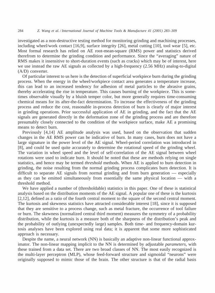
The experiment was carried out on a Norton Grinder. Fig. 1 shows the instrument set-up.Specifically, data from eight different experiments, involving an easy-to-grind bearing steel(52100), were collected. The system consists of the sensor, a preamplifier, a post amplifier anda data-acquisition system. The AE signal was received by a commercially available AE sensor(PAC U80D-87, whose frequency characteristics are known) that was mounted directly on theworkpiece via adhesive. The sensor’s AE signal was amplified by a preamplifier and a post ampli-


Fig. 1. Set-up of the AE test.

fier. The overall amplification factor for the grinding test was 40 dB. The data-acquision systemwas a Hewlett-Packard E1430A running in continuous-sampling mode at 2.56 MHz samplingrate. The A/D accuracy was 16 bits per sample, and appropriate anti-aliasing filtering was perfor-med internal to the HP system.

Grinding parameters were as follows:

O wheel peripheral speed — 2000 rev/min;O grind wheel type — aluminum oxide;O wheel diameter — 9.6 in;O workpiece feed rate — 103.7 in/min;O coolant — Master Chemical VHP 200, with flow rate of 0.88 gal/min.

Most parameters were kept constant among all tests, except that the depth of cut was varied.Generally, the more aggressive the cutting depth, the more likely burn was to occur.

Details of the tests are shown in Table 1. To show “burn” and “non-burn” signatures in thesame workpiece, in tests 4–8 the workpiece was ramped or tented as shown in the table. In thesecase, the depth of cut changed (piecewise) linearly.

All workpieces were examined post-mortem to check the condition, and signs of burn werenoted. The workpiece burn of steel 52100 is assayed visually and through laboratory testing. Thevisual burn location is indicated in Table 1. Both the surface hardness tests and the surface profile


Table 1The tests for the steel 52100 workpiece. All workpieces were 3.1 in long

Test Depth of cut (in) Cut profile Burn location (in) Comments

1 0.001 flat – no burn2 0.0005 flat – no burn3 0.003 flat 0.06-3 almost all burn4 0.002 flat 0.2-2.9 almost all burn5 0.0015-0.004 1.0-3 a ramp cut

6 0.001-0.004 1.25-3 a ramp cut

7 0.0003-0.0048-0.0003 0.2-2.8 a tent cut

8 0.0005-0.0045-0.0005 0.4-2.5 a tent cut

measurements were taken to provide burn-recognition information. At 32 equally spaced pointsalong each workpiece, a Leco M400-G2 Hardness Tester was used to record hardness values.The surface profile test was done by a computer-connected stylus surface measurement, and thesurface roughness values obtained were used to quantify the workpiece surface characteristics.

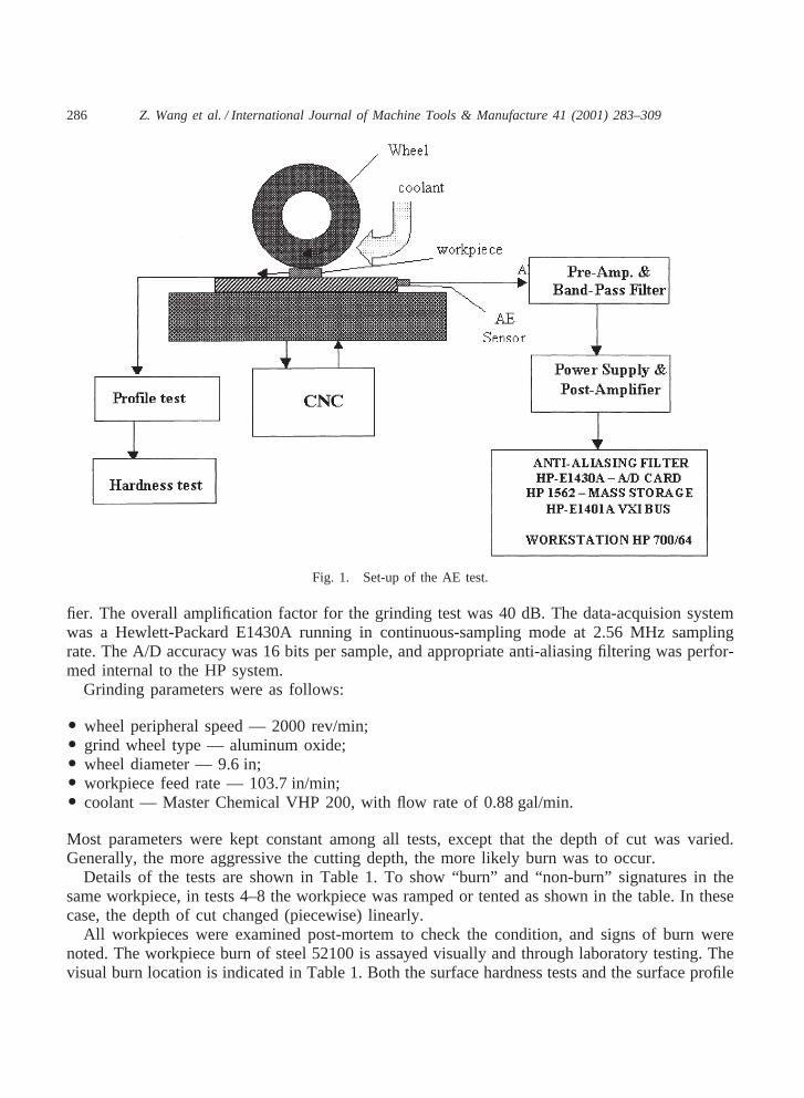
A typical AE trace observed and the corresponding power spectral density (PSD) are given inFig. 2. It would be ideal to have data about the original AE; that is, the acoustic signature fromthe zone of the wheel/workpiece interface. However, since the signal is distorted by the sensorcharacteristic (it is in fact a strongly narrowband filter), and more particularly since the AE mustpass through an unknown and changing medium involving the workpiece, coolant and apparatuson its way from the contact zone to the sensor, this is not reasonable.

3. Detection tools

3.1. What did not work

A number of statistics were applied individually to the collected data for detection of burn.For the most part these statistics were normalized, or otherwise rendered independent of the localAE power: the AE RMS power can rise or fall for reasons having little to do with grindingcondition, and in any case has been found to have limited predictive efficacy.

3.1.1. Zero-crossing rate (ZCR)“Count” technology is not new in AE applications [3]. As the name implies, this method counts

the number of zero-crossing events during each block of observed data. For a monochromaticsignal, twice the time between zero-crossings is the reciprocal of the frequency; for the compli-cated signals observed, the meaning is less clear. At any rate, little predictive capability was foundin this statistic.


Fig. 2. A typical “raw” AE trace (top) and the corresponding PSD spectrum (bottom) from the beginning of a grindingregime. Note that the spectrum is plotted logarithmically.

3.1.2. Ratio of power (ROP)It is natural to examine the behavior of the power spectrum of AE, with the idea that the

frequency behavior of “good” and “bad” grinding may differ. Thus, for each block of data, theROP was calculated from the normalized power spectrum as

ROP5On2

k5n1

uXku2/ON21

k50

uXku2, (1)

in which the denominator eliminates the effect of the local signal power. Here,N (N=1024) isthe chosen length of fast Fourier transform (FFT),Xk is thekth DFT output, and the summationis over any range of frequency, represented as from discrete Fourier transform (DFT) “bins”n1

to n2. A significant effort went toward identification of promising frequency bands (and indeedsets of bands), with little success. Our conclusion is that either the effect is small, or it is irretriev-ably lost due to the sensor characteristic.

3.1.3. Amplitude histogramThe amplitude histogram of each block data was obtained and analyzed. Effort was expended

to find the difference between the distributions, but no promising relationship was noted.


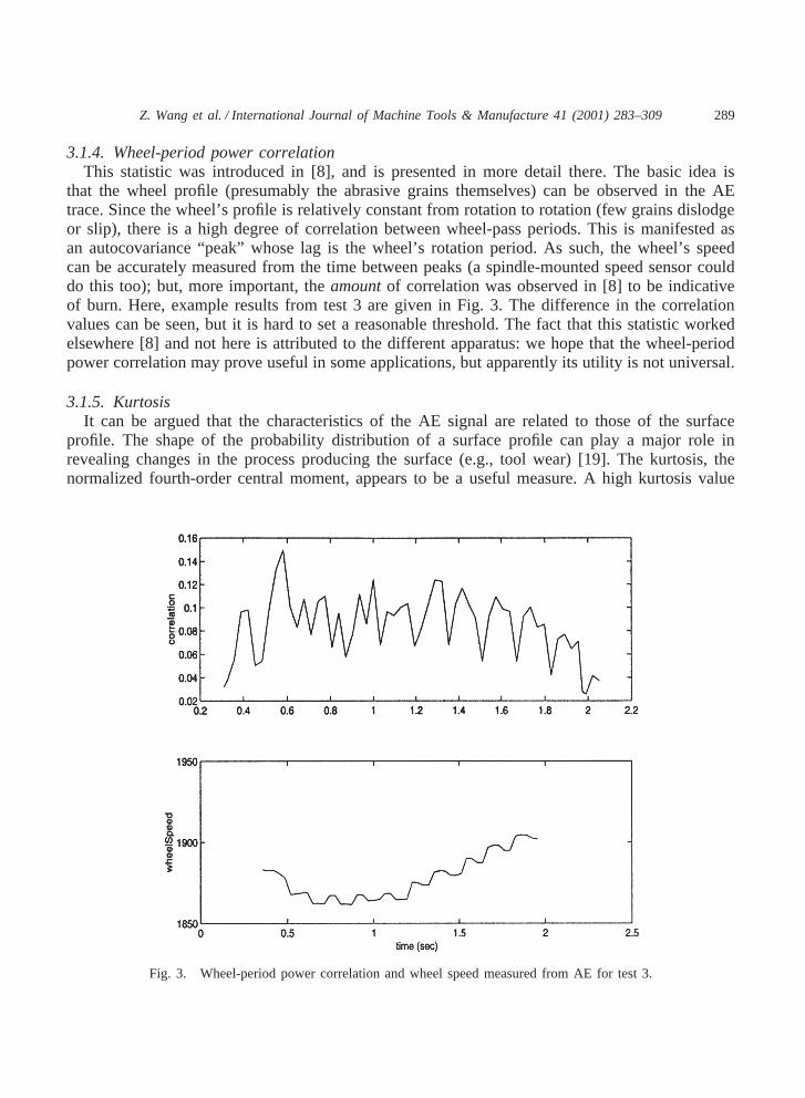
3.1.4. Wheel-period power correlationThis statistic was introduced in [8], and is presented in more detail there. The basic idea is

that the wheel profile (presumably the abrasive grains themselves) can be observed in the AEtrace. Since the wheel’s profile is relatively constant from rotation to rotation (few grains dislodgeor slip), there is a high degree of correlation between wheel-pass periods. This is manifested asan autocovariance “peak” whose lag is the wheel’s rotation period. As such, the wheel’s speedcan be accurately measured from the time between peaks (a spindle-mounted speed sensor coulddo this too); but, more important, theamountof correlation was observed in [8] to be indicativeof burn. Here, example results from test 3 are given in Fig. 3. The difference in the correlationvalues can be seen, but it is hard to set a reasonable threshold. The fact that this statistic workedelsewhere [8] and not here is attributed to the different apparatus: we hope that the wheel-periodpower correlation may prove useful in some applications, but apparently its utility is not universal.

3.1.5. KurtosisIt can be argued that the characteristics of the AE signal are related to those of the surface

profile. The shape of the probability distribution of a surface profile can play a major role inrevealing changes in the process producing the surface (e.g., tool wear) [19]. The kurtosis, thenormalized fourth-order central moment, appears to be a useful measure. A high kurtosis value

Fig. 3. Wheel-period power correlation and wheel speed measured from AE for test 3.


implies a sharp distribution peak and/or a high (relative to Gaussian) probability of observing anoutlying sample.

3.1.5.1. Time-domain kurtosis (TDK)Let xi, i=1, …,n, represent the real discrete AE data, andlet n be the number of data points of each block. The empirical kurtosis statistic [2] used in thispaper has the form

Kt5

1nO

n

i51

(xi−x̄)4

F1nO

n

i51

(xi−x̄)2G2, (2)

where x̄ is the empirical sample mean:

x̄51nO

n

i51

xi. (3)

In our implementation we usen=76,800, meaning that each block lasts 30 ms or approximatelyone rotation of the wheel. Based on our experimental results it was found that TDK is related toburn as shown in the upper plot of Fig. 4, but large variation was observed. The variations makeit difficult to set the reasonable threshold and certainly reduce the detection performance. TDKwill be used later as the input to the NN.

Fig. 4. TDK and FDK for test 6. Dashed vertical lines indicate the location of burn.


3.1.5.2. Frequency-domain kurtosis (FDK)Particularly if the time-domain signal contains tran-sient bursts of enhanced energy (e.g., from grain contact), higher-order moments of the complexfrequency components may contain additional information that could be utilized in detecting sig-nals. Thus we can compute the frequency-domain kurtosis (FDK) for the real or imaginary partsof the complex frequency components. The FDK [12,13] represents a measure for the probabilitydistribution over a time interval consisting ofN DFTs each of lengthM. The operation isdescribed as

Kf(k)5

1NO

N

q51

(Xk(q)−X̄k)4

F1NO

N

q51

(Xk(q)−X̄k)2G2, (4)

whereX̄k is the empirical sample mean

X̄k51NO

N

q51

Xk(p) (5)

andXk(q) is the real part of thekth DFT output of the segmentq, kP{1, M}. Only the real partwill be discussed here, and of course a similar analysis can be used with the imaginary part.

Our zero-mean raw AE signal was processed utilizing a 512-point FFT (M=512) and the FDKwas obtained by appropriately dealing with the 150 consecutive FFT outputs (N=300), giving anoverall time interval of 30 ms. The middle plot in Fig. 4, showing the FDK fork=60 (300 kHz),is typical: there is little predictive power. By contrast, the lowest plot in Fig. 4 shows the FDKfor k=256 — it appears that this result is similar to that for the TDK. The results of FDK withk=256 for different tests are shown in Fig. 5, which can provide useful information to indicateburn. However,k=256 corresponds to 1280 kHz (half the sampling rate, otherwise known asthe “folding frequency”) which is far out-of-band, Hence, while this is intriguing, it is mostlya curiosity.

3.2. What worked

3.2.1. CFAR power lawAs applied to the detection of transient events, a detector attracting much attention and interest

is Nuttall’s power-law statistic [22]

Tpl(X)5OM21

k50

Xnk, (6)

where theXk is the kth magnitude-squared FFT bin,n is a changeable exponent and 2M is thetotal number of FFT bins (due to conjugate symmetry, only half of the magnitude-squared FFTbins need be interrogated). Respectivelyn=1 and n=` correspond to the energy detector andmax{Xk}; 2,n,3 provides good performance in a wide range. Although it is effective in somemodels and easy to implement, this statistic relies on pre-normalized data. Due to the fluctuation


Fig. 5. FDK with k=256 for tests. Dashed vertical lines indicate the location of burn and dashed horizontal linesillustrate the possible threshold.

of the AE signal during the grinding process, a constant false alarm-rate (CFAR) power-law [23]statistic is used

Tcpl(X)5

OM21

k50

Xnk

SOM21

k50

XkDn, (7)

whereTcpl is clearly not affected by signal amplitude. WithM=32, for each time interval of 1ms, our {Xk} are taken as the PSD of the raw AE signal. The example results of power law andthe CFAR power law are compared in Fig. 6. To see the results more clearly, the averaged statisticvalue in each wheel rotation (the length is 30 ms) was used instead. The CFAR power law appears


Fig. 6. Results of power law and CFAR power law for test 8. Dashed vertical lines indicate the location of burn.From left to right,n is 0.5, 2.5 and̀ , respectively.

to be an effective method to detect burn; the unnormalized power-law statistic may indeed beinformative, but due to amplitude dependence its wide variation suggests that it is unsuitable.

3.2.2. MVDProcessed in the frequency domain, the CFAR mean-value deviance (MVD) statistic [6] is

defined as

Tmvd(X)51MOM21

k50

log[X̄/Xk], (8)

whereX̄ is the mean value of {Xk}; M and Xk have the same meanings as in the CFAR power-law statistics. The MVD statistic has been proved to be effective in the detection of transients insome applications. The MVD appears to be useful for burn detection.

3.2.3. Neural network detection scheme

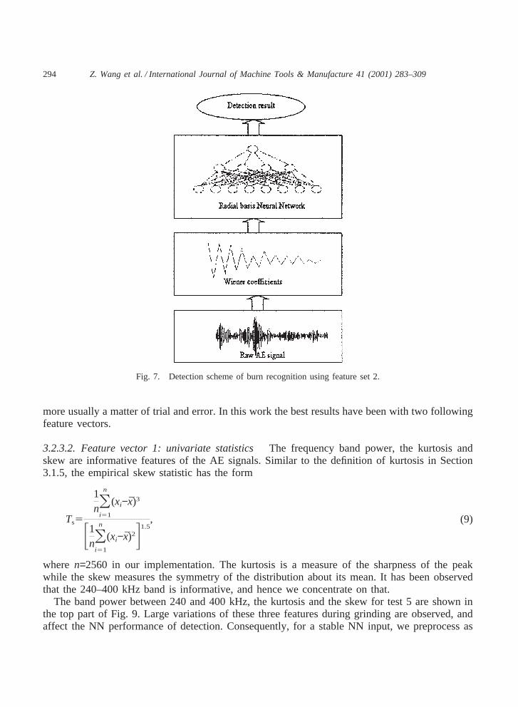
3.2.3.1. Feature selection The NN-based detection scheme is shown in Figs. 7 and 8. Theinputs in Fig. 7 are, in classification parlance, thefeatureson which a decision is to be based.These must be chosen judiciously and succinctly, since the selection of a set of features too greatfor the number of training data usually results in “overtraining”; that is, of the adaptation of theclassifier to spurious non-generalizable patterns [24]. Feature selection is at best an art, and is


Fig. 7. Detection scheme of burn recognition using feature set 2.

more usually a matter of trial and error. In this work the best results have been with two followingfeature vectors.

3.2.3.2. Feature vector 1: univariate statisticsThe frequency band power, the kurtosis andskew are informative features of the AE signals. Similar to the definition of kurtosis in Section3.1.5, the empirical skew statistic has the form

Ts5

1nO

n

i51

(xi−x̄)3

F1nO

n

i51

(xi−x̄)2G1.5, (9)

where n=2560 in our implementation. The kurtosis is a measure of the sharpness of the peakwhile the skew measures the symmetry of the distribution about its mean. It has been observedthat the 240–400 kHz band is informative, and hence we concentrate on that.

The band power between 240 and 400 kHz, the kurtosis and the skew for test 5 are shown inthe top part of Fig. 9. Large variations of these three features during grinding are observed, andaffect the NN performance of detection. Consequently, for a stable NN input, we preprocess as


Fig. 8. A generic radial basis network.

follows. For each specified block of AE signal, we calculate a feature series {T(i)}. For eachfeature series {T(i)} (this can refer to band power, kurtosis or skew), the mean and the standarddeviation are calculated to form the new features:

mT51lO

l

i51

T(i) (10)

and

sT5! 1l−1O

l

i51

(T(i)−mT)2, (11)

wherel is the window size. From the above process, the feature vectorV1 corresponding to bandpower, kurtosis and skew is extracted

V15{mp, mk, ms, sp, sk, ss}, (12)

wheremp, mk andms are the mean values of the frequency band power, kurtosis and skew; andsp, sk andss are the corresponding standard deviation values. The refined features of test 5 areplotted in the middle and bottom part of Fig. 7: it is clear that the values of the refined featuresfluctuate less. The window sizel is experimentally based, and is set to 30 in our actual use; thatis, each feature vector was extracted from a 30 ms block AE signal.


Fig. 9. Features for test 5 using band power, kurtosis and skew. The top three plots show the statistics themselvesas based on 1 ms block averages; the middle and lower plots are of means and standard deviations based onl=30blocks. These latter six features form feature set 1.

3.2.3.3. Feature vector 2: Wiener coefficientsIn the linear prediction problem it is desired toestimate thenth element of a time seriesx(n) using {x(m)} n−1

m=n−M — the previousM time samples.That is, the vectorh={ h(1), h(2), …, h(M)} which minimizes

E{[ x(n)2hTx(n)]2} 5EHFx(n)2OMk51

h(k)x(n2k)G2J (13)

is sought — this is a version of the Wiener filtering problem. It may appear strange to estimatex(n) based on theM prior samples when one could simply wait one sample and have it; but it is


the form of the filter which matters. In fact, the vectorh so derived coincides with that usedfor autoregressive (AR) and maximum entropy (ME) spectral modeling, in that the AR spectralestimate is

fARx (w)5

k

|1−OMk51

h(k) e−jwk|2 (14)

in which k is a proportionality constant. The Wiener/AR coefficients are also sometimes referredto as linear prediction coefficients (LPCs), and are used as signal descriptors both for speechcoding/compression and speech recognition. At any rate, the point is that the Wiener coefficientssummarize a considerable amount of spectral information in a relatively few numbers.

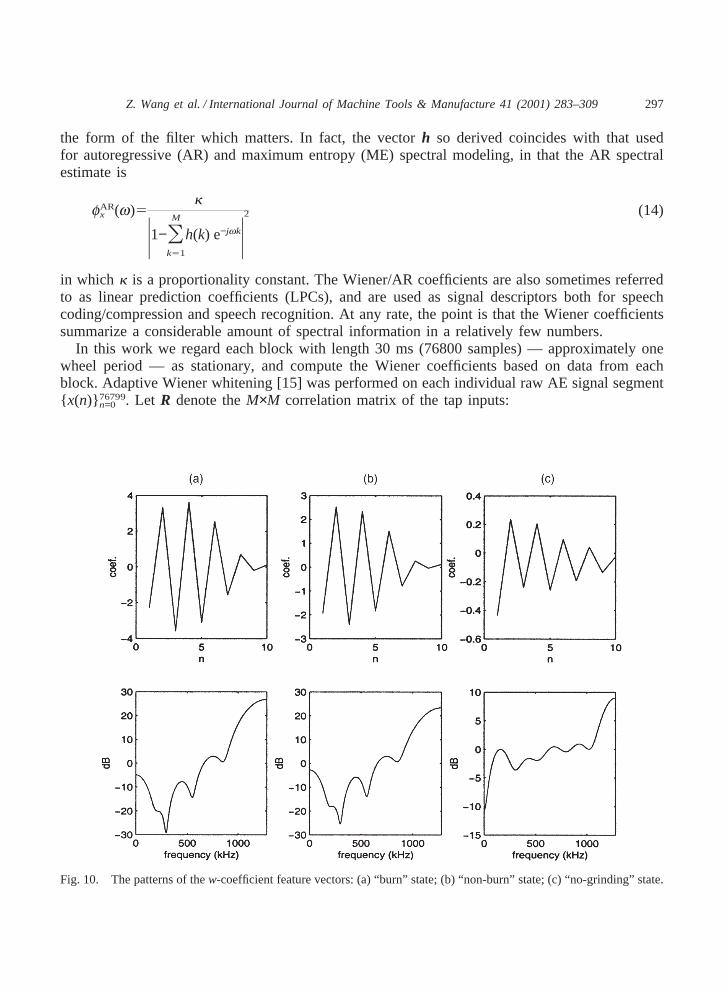
In this work we regard each block with length 30 ms (76800 samples) — approximately onewheel period — as stationary, and compute the Wiener coefficients based on data from eachblock. Adaptive Wiener whitening [15] was performed on each individual raw AE signal segment{ x(n)} 7679

n=09. Let R denote theM×M correlation matrix of the tap inputs:

Fig. 10. The patterns of thew-coefficient feature vectors: (a) “burn” state; (b) “non-burn” state; (c) “no-grinding” state.


R51r(0) r(1) … r(M−1)

r(1) r(0) … r(M−2)

: : ¢ :

r(M−1) r(M−2) … r(0)2, (15)

whereM is the filter order, and the autocorrelationr(·) is estimated as

r(k)5 ON2k21

n50

(x(n)x(n1k)). (16)

Correspondingly, letp denote theM×1 cross-correlation vector

p5[r(1)r(2)…r(M)]T. (17)

Thus, theM×1 coefficient vector of the Wiener filter is obtained by solving

Rh52p. (18)

While either matrix inversion or Gaussian elimination [O(M3)] are sufficient to solve for theWiener coefficients, a particularly efficientO(M2) algorithm due to Levinson and Durbin (again,see [15]) is also available. Fig. 10 shows a typical representation of the feature vectors reflectingthe “burn”, “non-burn” and “no-grinding” states. The vectors themselves are shown in the upperplots, and the corresponding AR spectra in the lower. Note that the AR orderM is determinedexperimentally. Various orders fromM=5 to 50 were assayed; it was found thatM=10 gave thebest results.

Fig. 11. The detection results of the radial basis NN and feed-forward NN for test 2.


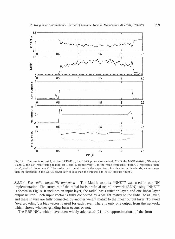
Fig. 12. The results of test 1, no burn. CFAR pl, the CFAR power-law method; MVD, the MVD statistic; NN output1 and 2, the NN result using feature set 1 and 2, respectively. 1 in the result represents “burn”, 0 represents “non-burn”, and21 “no-contact”. The dashed horizontal lines in the upper two plots denote the thresholds; values largerthan the threshold in the CFAR power law or less than the threshold in MVD indicate “burn”.

3.2.3.4. The radial basis NN approach The Matlab toolbox “NNET” was used in our NNimplementation. The structure of the radial basis artificial neural network (ANN) using “NNET”is shown in Fig. 8. It includes an input layer, the radial basis function layer, and one linear layeroutput neuron. Each input vector is fully connected by a weight matrix to the radial basis layer,and these in turn are fully connected by another weight matrix to the linear output layer. To avoid“overcrowding”, a bias vector is used for each layer. There is only one output from the network,which shows whether grinding burn occurs or not.

The RBF NNs, which have been widely advocated [21], are approximations of the form


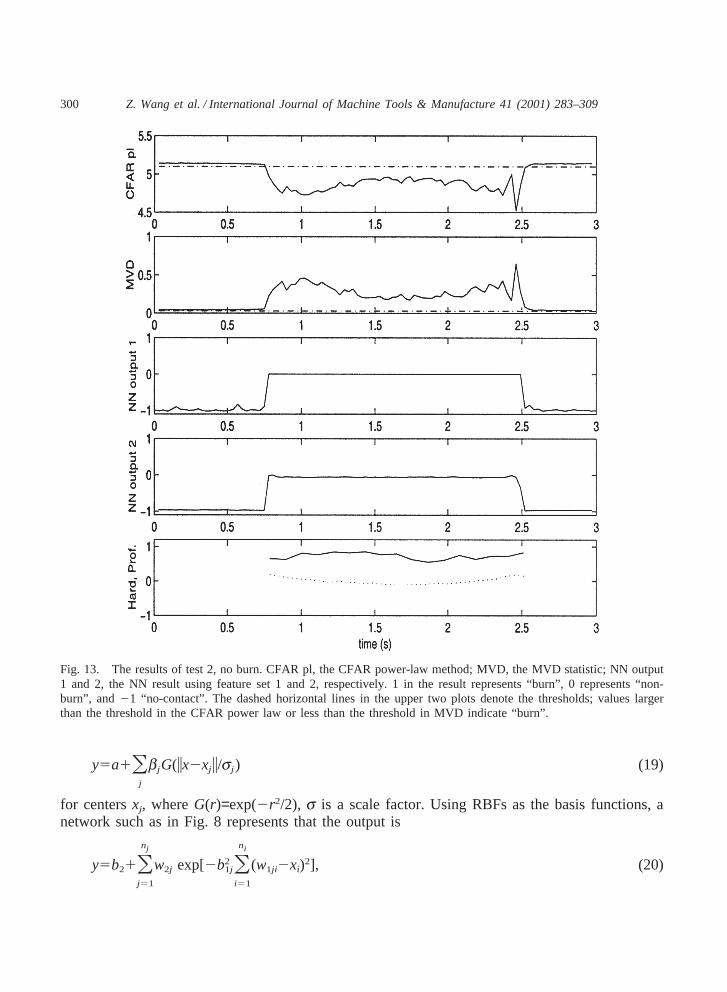
Fig. 13. The results of test 2, no burn. CFAR pl, the CFAR power-law method; MVD, the MVD statistic; NN output1 and 2, the NN result using feature set 1 and 2, respectively. 1 in the result represents “burn”, 0 represents “non-burn”, and21 “no-contact”. The dashed horizontal lines in the upper two plots denote the thresholds; values largerthan the threshold in the CFAR power law or less than the threshold in MVD indicate “burn”.

y5a1Oj

bjG(ix2xj i/sj ) (19)

for centersxj, whereG(r)=exp(2r2/2), s is a scale factor. Using RBFs as the basis functions, anetwork such as in Fig. 8 represents that the output is

y5b21Onj

j51

w2j exp[2b21jOni

i51

(w1ji2xi)2], (20)


Fig. 14. The results of test 3, heavy burn. CFAR pl, the CFAR power-law method; MVD, the MVD statistic; NNoutput 1 and 2, the NN result using feature set 1 and 2, respectively. 1 in the result represents “burn”, 0 represents“non-burn”, and21 “no-contact”. The dashed vertical lines indicate burn location observed visually; the dashed horizon-tal lines in the upper two plots denote the thresholds. Values larger than the threshold in the CFAR power law or lessthan the threshold in MVD indicate “burn”.

wherex is the input vector with sizeni×1, ni andnj are separately the numbers of neurons usedin the input and “hidden” layers. The trainable parametersw1 and b1 are, respectively, annj×ni

weight matrix and thenj×1 bias vector for the hidden layer, andw2 andb2 are the corresponding1×nj weight matrix and scalar bias for the linear (output) layer.

The NN is established through the training phase. The number of neurons used in the radialbasis layer,nj, was originally set as 1 and increased by one each time until performance wasacceptable. The actual error is defined as the sum of the squared differences between the desiredoutput and the actual output over a specified number of input vectors. During this development


Fig. 15. The results of test 4, heavy burn. CFAR pl, the CFAR power-law method; MVD, the MVD statistic; NNoutput 1 and 2, the NN result using feature set 1 and 2, respectively. 1 in the result represents “burn”, 0 represents“non-burn”, and21 “no-contact”. The dashed vertical lines indicate burn location observed visually; the dashed horizon-tal lines in the upper two plots denote the thresholds. Values larger than the threshold in the CFAR power law or lessthan the threshold in MVD indicate “burn”.

process, the network modifies the connections between individual processing neurons, representedby w1, w2, b1 andb2.

Just as in any statistical analysis, an implied requirement for developing robust neural networkmodels is that the training sets cover as many of the possible variations in the input and outputvector as feasible. For practical considerations, a limited number of samples should be used. Thuscare must be taken when choosing the training set to ensure that it be broad-based. There arethree possible distinguished states during the grinding process: the no (workpiece/wheel) contact


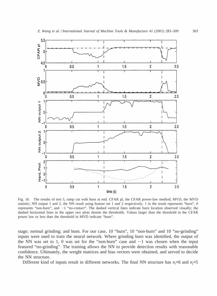
Fig. 16. The results of test 5, ramp cut with burn at end. CFAR pl, the CFAR power-law method; MVD, the MVDstatistic; NN output 1 and 2, the NN result using feature set 1 and 2 respectively. 1 in the result represents “burn”, 0represents “non-burn”, and21 “no-contact”. The dashed vertical lines indicate burn location observed visually; thedashed horizontal lines in the upper two plots denote the thresholds. Values larger than the threshold in the CFARpower law or less than the threshold in MVD indicate “burn”.

stage; normal grinding; and burn. For our case, 10 “burn”, 10 “non-burn” and 10 “no-grinding”inputs were used to train the neural network. Where grinding burn was identified, the output ofthe NN was set to 1, 0 was set for the “non-burn” case and21 was chosen when the inputfeatured “no-grinding”. The training allows the NN to provide detection results with reasonableconfidence. Ultimately, the weight matrices and bias vectors were obtained, and served to decidethe NN structure.

Different kind of inputs result in different networks. The final NN structure hasni=6 andnj=5


Fig. 17. The results of test 6, ramp cut with burn at end. CFAR pl, the CFAR power-law method; MVD, the MVDstatistic; NN output 1 and 2, the NN result using feature set 1 and 2, respectively. 1 in the result represents “burn”, 0represents “non-burn”, and21 “no-contact”. The dashed vertical lines indicate burn location observed visually; thedashed horizontal lines in the upper two plots denote the thresholds. Values larger than the threshold in the CFARpower law or less than the threshold in MVD indicate “burn”.

when we used the feature vectorV1 as inputs. Otherwise, if the inputs was taken as the featurevectorV2 (the AR coefficients), the radial basis network utilized consists ofni=10 neurons in theinput layer andnj=3 neurons in the radial basis layer. The two radial basis networks have beenused successfully to detect grinding burn. If the value of the output was larger than 0.5, grindingburn was declared. The closer to 1 the output, the more confident the burn detection. The closerto 0 the output, the more it is possible to declare “non-burn”.

Finally, a usually worthy competitor to the RBF NN is the perhaps more popular MLP feed-


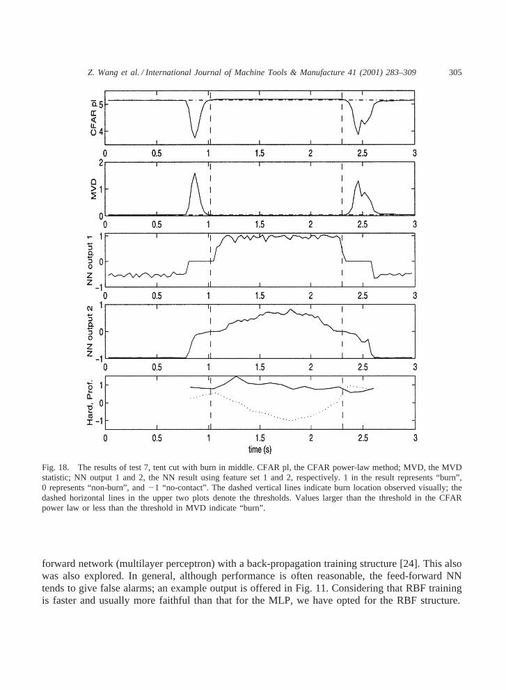
Fig. 18. The results of test 7, tent cut with burn in middle. CFAR pl, the CFAR power-law method; MVD, the MVDstatistic; NN output 1 and 2, the NN result using feature set 1 and 2, respectively. 1 in the result represents “burn”,0 represents “non-burn”, and21 “no-contact”. The dashed vertical lines indicate burn location observed visually; thedashed horizontal lines in the upper two plots denote the thresholds. Values larger than the threshold in the CFARpower law or less than the threshold in MVD indicate “burn”.

forward network (multilayer perceptron) with a back-propagation training structure [24]. This alsowas also explored. In general, although performance is often reasonable, the feed-forward NNtends to give false alarms; an example output is offered in Fig. 11. Considering that RBF trainingis faster and usually more faithful than that for the MLP, we have opted for the RBF structure.


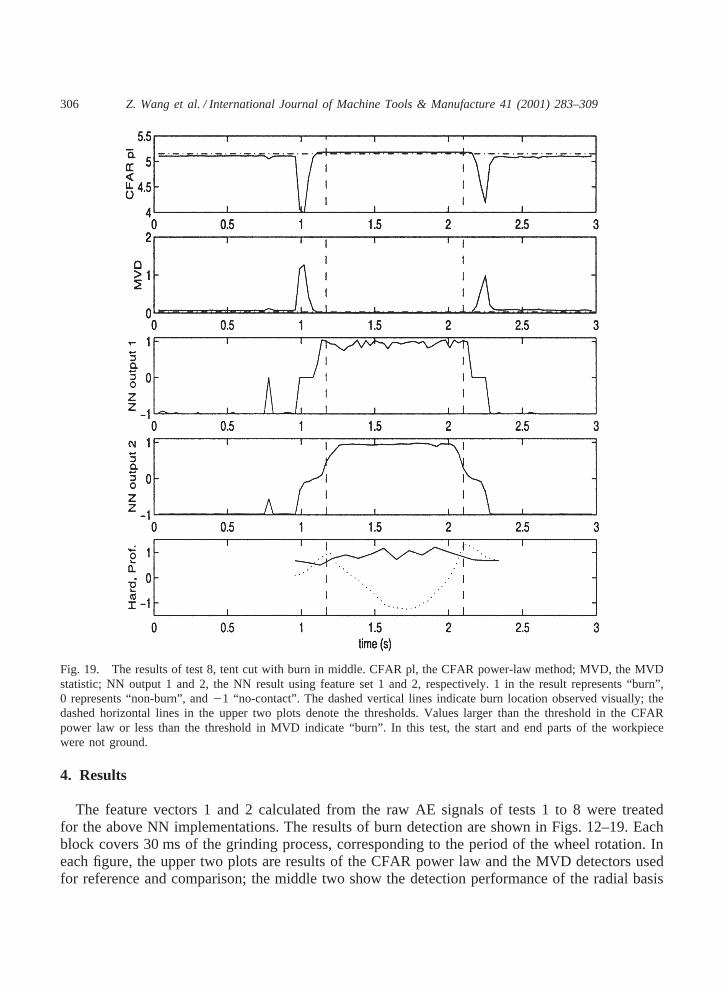
Fig. 19. The results of test 8, tent cut with burn in middle. CFAR pl, the CFAR power-law method; MVD, the MVDstatistic; NN output 1 and 2, the NN result using feature set 1 and 2, respectively. 1 in the result represents “burn”,0 represents “non-burn”, and21 “no-contact”. The dashed vertical lines indicate burn location observed visually; thedashed horizontal lines in the upper two plots denote the thresholds. Values larger than the threshold in the CFARpower law or less than the threshold in MVD indicate “burn”. In this test, the start and end parts of the workpiecewere not ground.

4. Results

The feature vectors 1 and 2 calculated from the raw AE signals of tests 1 to 8 were treatedfor the above NN implementations. The results of burn detection are shown in Figs. 12–19. Eachblock covers 30 ms of the grinding process, corresponding to the period of the wheel rotation. Ineach figure, the upper two plots are results of the CFAR power law and the MVD detectors usedfor reference and comparison; the middle two show the detection performance of the radial basis


networks, where “NN output 1” indicates the output of the network using feature vectorV1 asinputs and “NN output 2” is the output of the network using feature vectorV2. The lowest plotin each shows the results from the post hardness and profile tests, which can identify cases of burnand non-burn. The hardness and the profile values are normalized by 1000 and 0.002, respectively.

We can see that the CFAR power-law and the MVD methods provide useful information aboutburn. Based on our experiment, we set 5.15 as the threshold of the CFAR power law withn=0.5and 0.05 as the threshold of the MVD detector. Burn is declared if the value of the CFAR power-law method is larger than 5.15 or the MVD value is less than 0.05. As with any threshold detec-tors, there is the disadvantage that the setting of the threshold is experience-based and may besituation-dependent. It was noted that the value difference between the “no-grinding” signal andthe “burn” signal is quite small; in the NN approach, there is no such concern.

It is easily noticed that the NN shows effective performance in all tests. It is clear from the posthardness and profile tests that the NN method indicates a “burn” signature before the occurrence ofthe true burn — a particularly useful characteristic. Note that despite the NN having been trainedwith but 30 samples (10 from each regime), the performance over the much larger test data setis remarkably stable: for feature sets 1 and 2, the plots show the NN outputs given at respectively30 ms and 3 ms intervals!

Fig. 20. A distorted AE signal due to preamplifier overload.


5. Summary

The goal has been to detect abnormal grinding conditions via appropriate digital signal pro-cessing of acoustic emission (AE) data, this information being sampled at a high (2.56 MHz) rateand used in its raw (i.e., not RMS) form. The data were collected from a sequence of tests on52100 bearing steel and a variety of conditions; the workpieces were assayed post-mortem fortheir quality, so that this could be compared with the AE collected.

For the most part, the “threshold”-oriented statistical tools — that is, those which digest thedata to a single statistic to be compared with some preset value — were found to have limitedability in predicting grinding state. Exceptions to this include certain statistical tools recentlyfinding application in the identification of transient events, particularly in sonar. The efficacy ofthese tools is intriguing, but for the most part they are eclipsed by a neural network approachbased on the fast-training radial basis function (RBF) architecture. For these, despite training ona remarkably small set, identification of burn over a much larger test set is essentially perfect.Two families of “feature vectors” (inputs to the neural networks) are employed, one based onautoregressive parameters and the other on a vector of averaged statistical properties. In bothcases the performance is good, and there does not seem to be a reason to prefer one over the other.

Acknowledgements

This research was supported by the National Science Foundation under contract DMI-9634859.

Appendix A. Note about distortion

There are some remarks about a somewhat obscure form of distortion in [17], and since thiskind of distortion was indeed observed in the early phases of our work we would like to reporton it here in the hope that other researchers may avoid the problem.

The AE signals originating from the grinding zone were occasionally quite strong, and suchhigh-amplitude signals could cause overload in the preamplifier and distortion of the signals, asshown in Fig. 20. One might expect an amplifier overload to be accompanied by a saturated or“clamped” output, and thus be easily discernible. But when the overload is of significant durationand there is a high-pass (or bandpass) filter between the overloaded amplifier and the point ofobservation, the effect is less clear. In fact, what is observed is an interval initially resemblingthe impulse response of the filter, and then with no signal at all. An example is shown in Fig. 20.

References

[1] P. Akerberg, B. Jansen, Neural net-based monitoring of steel beams, Journal of The Acoustical Society of America98 (1995) 1505–1509.

[2] K. Balanda, H. MacGillivray, Kurtosis: a critical review, The American Statistician 42 (2) (1988) 111–119.


[3] J. Baron, S. Ying, Acoustic emission source location, in: Nondestructive Testing Handbook, second ed., vol. 5,American Society for Nondestructive Testing, Columbus, Ohio, USA, 1987.

[4] T. Blum, M. Tomizuka, Grinding process feedback using acoustic emission, University of California (Berkeley)Engineering Science Research Center (ESRC) Technical Report 90–19, September, 1990.

[5] T. Carolan, S. Kidd, D. Hand, Acoustic emission monitoring of tool wear during the face milling of steels andaluminium alloys using a fibre optic sensor. Part 2: Frequency analysis, Proceedings of the Institution of Mechan-ical Engineers, Part B 211 (1997) 311–319.

[6] B. Chen, P. Willett, R. Streit, Transient detection using a homogeneity test, in: Proceedings of 1999 ICASSP,Phoenix, AZ, March, 1999, no. 1715, IEEE, Piscataway, New Jersey.

[7] X. Chen, W. Rowe, Y. Li, Grinding vibration detection using a neural network, Proceedings of the Institution ofMechanical Engineers, Part B 210 (4) (1996) 349–352.

[8] P. DeAguiar, P. Willett, J. Webster, Acoustic emission applied to detect workpiece burn during grinding, in: S.Vahaviolos (Ed.), Acoustic Emission: Standards and Technology Update, vol. STPB53, ASTM, West Conso-hocken, Pennsylvania, 1999, 107–124.

[9] J. Dong, J. Webster, P. Willett, Application of AE to wheel/work and wheel/truer contact detection in high-speedcylindrical grinding operations, in: Report 3, University of Connecticut Grinding Center, Storrs, CT, 1995. IEEE,Piscataway, New Jersey.

[10] D. Dornfeld, In-process recognition of cutting states, JSME International Journal 37 (4) (1994) 638–650.[11] D. Dornfeld, H. Cai, An investigation of grinding and wheel loading using acoustic emission, Transactions of the

ASME, Journal of Engineering for Industry 106 (1984) 28–33.[12] R. Dwyer, Use of the kurtosis statistic in the frequency domain as an aid in detecting random signals, IEEE

Journal of Oceanic Engineering OE9 (2) (1984) 85–92.[13] R. Dwyer, Detection on non-Gaussian signals by frequency domain kurtosis estimation, in: Proceedings of 1983

ICASSP, 1983, pp. 608–610.[14] H. Eda, K. Kishi, H. Ueno, K. Kakino, A. Fujiwara, In-process detection of grinding burns by means of utilizing

acoustic emission, Bulletin of JSPE 18 (4) (1984) 299–304.[15] S. Haykin, Adaptive Filter Theory third ed., Prentice-Hall, Upper Saddle River, New Jersey, 1996.[16] I. Inasaki, Monitoring of dressing and grinding processes with acoustic emission signals, Annals of the CIRP 34

(1) (1985) 277–280.[17] K. Jemielniak, Some aspects of acoustic emission signal processing, in: CIRP 1997 January Meeting, Technische

Rundschau, Berne, Switzerland, 1997 STC-C.[18] K. Jemielniak, O. Otman, Tool failure detection based on analysis of acoustic emission signals, Journal of Materials

Processing Technology 76 (1998) 192–197.[19] E. Kannatey-Asibu Jr., D. Dornfeld, A study of tool wear using statistical analysis of metal-cutting acoustic

emission, Wear 76 (1982) 247–261.[20] K. Mori, N. Kasashima, T. Yamane, T. Nakai, An intelligent vibration diagnostic system for cylindrical grinding,

in: Japan/USA Symposium on Flexible Automation, vol. 2, 1992, pp. 1097–1100.[21] M. Musavi, W. Ahmed, K. Chan, K. Faris, On the training of radial basis function classifiers, Neural Networks

5 (1992) 595–603.[22] A. Nuttall, Detection performance of power-law processors for random signals of unknown location, structure,

extent and strength, in: NUWC-NPT Technical Report 10,751, Naval Undersea Warfare Center, Division Newport,Rhode Island, USA, 1994.

[23] A. Nuttall, Performance of power-law processors with normalization for random signals of unknown structure,in: NUWC-NPT Technical Report 10,760, Naval Undersea Warfare Center, Division Newport, Rhode Island,USA, 1997

[24] B. Ripley, Pattern Recognition and Neural Networks, Cambridge University Press, 1997.[25] J. Walker, S. Russell, G. Workman, Neural network/acoustic emission burst pressure prediction for impact dam-

aged composite pressure vessels, Material Evaluation 55 (1997) 903–907.[26] J. Webster, I. Marinescu, R. Bennett, Acoustic emission for process control and monitoring of surface integrity

during grinding, Annals of the CIRP 43 (1994) 299–304.[27] S. Wilcox, R. Reuben, The detection of short time-scale tool degradation events during face milling operations

using cutting force and AE, Proceedings of the Institution of Mechanical Engineers, Part B 208 (3) (1994) 205–215.

Neural network detection of grinding burn from acoustic ...

Documents

Transcript of Neural network detection of grinding burn from acoustic ...