MMAE540 Robotics- Class Project Paper

Neural Network Controller for Robotic Manipulator

Kai Qian1

1Department of Biomedical Engineering, Illinois Institute of Technology, Chicago, IL 60616 USA

1. Introduction

Artificial neural network is parallel computation structure inspired from the understanding of biological

nervous system(Lippmann, 1987). It consists of many interconnected computational element through

weights which keep adapting to achieve better system response. Two major capacities of neural network

are classification (Ripley, 1994), a simple example is just perceptron, and function fitting (can map from

space m nR toR ), such as multilayer neural network. It has been shown a two-layer networks with sigmoid

function activation function for hidden layer and linear activation function for output layer, can

approximate any continuous function to any degree of accuracy with sufficient large number of hidden

layer nodes(Hornik et al., 1989). Based on its universal approximation capacity neural network has been

naturally and successfully applied to identification and control of complex system dynamics(Hagan et al.,

2002).

For robotic manipulator control, the adaptive controller(Slotine and Li, 1991) we studied in class has

shown impressive asymptotic trajectory tracking performance in face of parameters uncertainty such as

loads changes. Without knowing the mass, link length and load information, the controller estimates those

parameters and makes them converge to its real value, therefore provide perfect estimation of system

dynamic to achieve the great system performance. The adaptive control scheme(Slotine and Weiping Li,

1987) is shown in figure 1.

Figure 1. Adaptive control scheme for robotic manipulator(Slotine and Weiping Li, 1987).

In deriving adaptive controller, it requires substantial work to compute the Y matrix, such that

ˆˆˆ( , , , ) ( ) ( , ) ( )r r r rY q q q q a H q q C q q q G q= + + . System performance depends on the accuracy of

regression matrix Y and the knowledge of complete system dynamics. However the estimation of the

adaptive controller reminded me the function approximation ability of neural network. It can give great

estimation only by training on input and output. If a neural network can replace the role of Y matrix, then

good system performance will be achieved as adaptive controller without preliminary dynamics analysis

to compute Y. This is also the motivation for this class project paper. From the literature search, the

paper(Lewis et al., 1996) was about the same objective with formal stability proof of the neural network

controller. The control scheme was shown in figure 2.

Figure 2. Neural network control Scheme for robotic manipulator(Lewis et al., 1996)

So, the neural network controller developed in this paper was based on this paper. The detailed derivation

was given in section 2 method part. And a 2-link manipulator tracking task simulation was used to

demonstrate the performance of the neural network controller. The properties and some considerations on

above neural network controller was followed in final discussion part.

2. Method

2.1. Neural Network

A three layer neural network as figure 3 with sigmoid activation function for input layer and linear activation function for output layer is defined by ( )T Ty W V xσ= (1)

1( ) sigmoid1 zz

eασ =

+

where V is NN input layer weights matrix, and W is output layer weights matrix. Output vector y is in m dimensions, which is also corresponding to the output layer neuron number N3, N3=m, and input layer vector x is in n dimensions, input layer number N1 = n, A general function f(x) can be written as

( ) ( )T Tf x W V xσ ε= + (2) ε is NN function reconstruction error. Since any continuous smooth function can be approximated by a large multilayer net based on various activation function, such as sigmoid and radial basis functions(Cybenko, 1989, Hornik et al., 1989). There exist finite hidden neuron number N2 , W and V to make the function reconstruction error ε very small. ( )f x will provide a best fit for target function.

y1

y2

Figure 3. Three Layers Neural Network Structure

2.2 Robotic Manipulator Dynamics

A general n-link robotic manipulator dynamic equation is given by

( ) ( , ) ( ) ( )m dM q q V q q q G q F q τ τ+ + + + = (3)

( ) ( ) ( )de t q t q t= − (4)

r e e= +Λ (5) ( )dq t is the desired trajectory input, e(t) is the tracking error and r(t) is the filtered tracking error. And

rearrange the system equation (3) with (4) (5), the manipulator dynamic equation can be expressed in term of filtered tracking error r as

m dMr V r fτ τ= − − + + (6)

( ) ( )( ) ( , )( ) ( ) ( )d m df x M q q e V q q q e G q F q= +Λ + +Λ + + (7) [ , , , , ]T T T T T T

d d dx e e q q q= (8) We choose control torque input to be

ˆvf K rτ = + (9)

where f is an estimation of f, then the system dynamic equation in term of filtered tracking error can be written as

( )v m dMr K V r f τ= − + + + (10)

ˆf f f= − (11) Based the feedback filtered tracking error dynamic equation (10), if function estimates error of f(t) is small and system disturbance is small, then a good tracking performance will be achieved(Dawson et al.,

1998). So, the essential part of the neural network controller in this paper is using neural network to approximate function f(t) to achieve better tracking performance.

2.3 Neural Network Controller A

Given neural network estimation of f as in (7) by

ˆ ˆˆ( ) ( )T Tf x W V xσ= (12)

where W and V are weights estimates and let W and V be the “ideal weights” with which the neural network reconstruction error will be minimal.

Assume ideal weights are bounded, desired trajectory input is bounded and the input vector x to neural network is bounded.

2, ( )TMF F

Z Z Z trace Z Z≤ = (13)

d

d d

d

qq Qq

≤

(14)

1 2dx c Q c r≤ + (15)

1 2, , ,d mc c Q Z are constants. Define the hidden-layer output error by

ˆˆ ( ) ( )T TV x V xσ σ σ σ σ= − = − (16) and with Taylor series expansion expressed by

2ˆˆ( ) ( ) '( ) ( )T T T T TV x V x V x V x V xσ σ σ= + +Ο (17) Since the activation function is sigmoid function, the higher order term in (17) is bounded by

23 4 5( )T

d F FV x c c Q V c V rΟ ≤ + + (18)

Let control input be

ˆˆ= ( )+T TvW V x K r vτ σ − (19)

Substitute (12)(17)(19) into (10) finally we will get

1ˆˆˆ( ) 'T T T

v mMr K V r W W V x w vσ σ= − + + + + + (20)

21 ˆ ' ( ) ( )T T T T

dw W V x W V xσ ε τ= + Ο + + (21)

1w is the disturbance term containing neural network reconstruction error, higher order term in Taylor expansion of sigmoid function, and system disturbance.

Assume 1w and v is zero, given the weight updated law by

ˆ ˆ

ˆˆ ˆ( ( ') )

T

T T

W F r

V Gx diag W r

σ

σ

=

=

(22)

F and G are positive definite Matrice. And choose Lyapunov function to be

1 11 1 1( ) ( )2 2 2

T T TL r Mr trace W F W trace V G V− −= + + (23)

1 11 ( ) ( )2

T T T TL r Mr r Mr trace W F W trace V G V− −= + + + (24)

Using (20) and let w1 and v to be zero, with the weights updating law, finally we will get

0TvL r K r= − ≤ (25)

As t increases, tracking error will approach zero. Formula (19) and (22) defined the Neural Controller A, however, the error tracking performance is based on three strong assumptions 1) no neural network estimation error 2) No unmodeled disturbance 3) No higher-order Taylor series term. Furthermore, no information is provided on weights updating stability. These limitations make the neural network controller A less appealing.

Neural controller B was proposed to overcome above limitations with weights updating law by

ˆˆˆ ˆˆ ( ')

ˆˆˆ ˆ( ( ') )

T T T

T T

W F r Fdiag V xr F r W

V Gx diag W r G r V

σ σ κ

σ κ

= − −

= −

(26)

where κ is constant. Add one robustifying term v(t)

ˆ( ) ( )z MFv t K Z Z r= − + (27)

zK is another design constant. Let the control law of neural controller B be

ˆˆ= ( )+T TvW V x K r vτ σ − (28)

Choosing the same Lyapunov function as (23), differentiating and substituting system dynamic equation (20) without assuming w1 = 0, yields

1

1

1 ˆˆˆ ( 2 ) ( ' )2

ˆ ˆ +trace ( ') ( )

Tv

T T T T Tm

T T T T

L r K r

r M V r traceW F W r V xr

V G V xr W r w v

σ σ

σ

−

−

= −

+ − + + −

+ + +

(29)

Through several inequality equations, it gives

0 1min[ ( ) ]Mv F F F

L r K r Z Z Z C C Zκ≤ − + − − − (30)

0 1min [ ( ) ] 0

0

Mv F F Fif K r Z Z Z C C Z

then L

κ+ − − − ≥

≤

(31)

Rearranging (31),

23 0

min

/ 4r

v

C Cr bK

κ +> ≡ (32)

Or

23 3 0/ 2 / 4 / zF

Z C C C bκ> + + ≡ (33)

where the minvK is the minimal element in the diagonal gain matrix, and constants in (32)(33) are from

bounded input, bounded ideal weight, and bonded higher order term in σ function Taylor series expansion assumptions as in (14)(15)(18) . (32)(33)(31) state that based on neural controller B (defined by (26)(27(28)), L is negative outside a compact set. If tracking error is outside of the compact set, L will become less than zero, system energy decreases and tends to drive r back to the compact set. And the

same explanation applies to the weights matrix. Therefore, neural controller B will guaranty the tracking error is bounded and weights updating is bounded. And the compact set range or tracking error range is adjustable by changing gain vK and those bounded constants as in (32)(33).

Since neural network controller B can provide bounded tracking error and weights tuning, it was adopted for the following simulation study section.

3. Simulation Results

Neural network controller B was implemented and simulated for a 2-link planar arm that is the same as

homework 6, with m1 = m2 = 5, l1 = l2 = 1, lc1=lc2=0.5 as shown in figure 4.

Figure 4. two-link planar

3.1 Neural Network Controller B vs. PD controller

The task is joints angle tracking as the desired trajectory given by 1 2sin(2 ), 2 sin( )d dq t q t= = , with

initial condition 1 2(0) 45 , (0) 45q q= − = . The tracking performance of neural controller B is shown in figure 5. The parameters for the controller are Kv = 20, Kz = 0.2, Zm = 400, Λ=[5 0;0 5], Initial Weights W , V sets to zero, F=diag(100*ones(80,1)), G=diag(100*ones(11,1)), neural network input layer neuron number N1=11, as the input vector given by

[1, , , , , ]T T T T T Td d dx e e q q q= (34)

Constant 1 in x vector is corresponding to the threshold vector which is the first column of weights matrix V. As shown in figure 5, neural network controller B achieved good performance for the tracking task;

only very small tracking error was observed (less than 0.08 rad).

Figure 5. Response of Neural Controller B

Figure 6. Response of PD Controller without Neural Network Part

For PD controller, the control torque input generated by Neural Network part is removed. All the other parameters left unchanged. The system output was shown in figure 6. The system tracking performance degrades a lot. Large tracking error and phase shift were observed. When PD controller gains Kv increased from 20 to 240, the system response was as in figure 7. Tracking error still could be observed clearly from the figure 7. Control torque input graphs for neural network controller B and PD controller with large gain were shown in figure 8. Oscillations were observed in torques generated by neural network controller B. Magnitude of the torque generated by PD controller was larger than that of neural network controller B.

0 2 4 6 8 10 12 14 16 18 20-2.5

-2

-1.5

-1

-0.5

0

0.5

1

1.5

2

2.5

time (s)

Join

t Ang

le (r

ad)

q1dq1q2dq2

0 2 4 6 8 10 12 14 16 18 20-4

-3

-2

-1

0

1

2

3

4

time (s)

Join

t Ang

le (r

ad)

q1dq1q2dq2

Figure 7. Response of PD Controller with large PD gains (Kv=240)

a) Torque generated by neural network controller B

b) Torque generated by PD controller with large gain

Figure 8. Torque generated by neural network controller B and PD controller with large gain

3.2 Comparison to adaptive controller

The adaptive controller used here was the same as in homework 6 with the following parameters, Kd = 20, Lambda = diag([5,5]) P=diag([4, 2, 1, 20, 8] . The response of the adaptive controller was shown in figure 9. The a vector estimation was as figure 10.

0 2 4 6 8 10 12 14 16 18 20-2.5

-2

-1.5

-1

-0.5

0

0.5

1

1.5

2

2.5

time (s)

Join

t Ang

le (r

ad)

q1dq1q2dq2

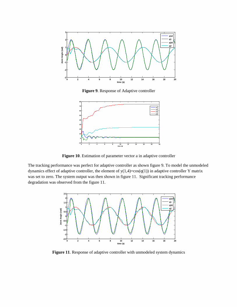
Figure 9. Response of Adaptive controller

Figure 10. Estimation of parameter vector a in adaptive controller

The tracking performance was perfect for adaptive controller as shown figure 9. To model the unmodeled dynamics effect of adaptive controller, the element of y(1,4)=cos(q(1)) in adaptive controller Y matrix was set to zero. The system output was then shown in figure 11. Significant tracking performance degradation was observed from the figure 11.

Figure 11. Response of adaptive controller with unmodeled system dynamics

0 2 4 6 8 10 12 14 16 18 20-3

-2

-1

0

1

2

3

time (s)

Join

t Ang

le (r

ad)

q1dq1q2dq2

0 2 4 6 8 10 12 14 16 18 20-10

0

10

20

30

40

50

60

70

80

time (s)

a1a2a3a4

0 2 4 6 8 10 12 14 16 18 20-2.5

-2

-1.5

-1

-0.5

0

0.5

1

1.5

2

2.5

time (s)

Join

t Ang

le (r

ad)

q1dq1q2dq2

3.3 Neural Network Controller B with less number of nodes in hidden layer

The neural network controller B with 80 nodes in hidden layer gave good tracking performance as figure 5. To reduce the number of nodes in hidden layer will increase the estimation error of the neural network, which then increases the bound of the tracking error as (32). A neural network controller with the same parameters as in section 3.1 but the number of nodes in hidden layer was reduced to 20. The response was shown in figure 12. As expected, larger tracking error was observed compared with figure 5.

Figure 12. Neural Network Controller B with fewer nodes in hidden layer

3.4 Neural Network Controller A

Neural network controller A based on (19)(22) with w1(t)=0,v(t)=0, Kv = 20, Λ=[5 0;0 5], Initial Weights W , V sets to zero, F=diag(100*ones(80,1)), G=diag(100*ones(11,1)) was also simulated to compare with NN controller B. The response and torque plot were as figure 13 and figure 14. Since the strong assumptions of neural network controller A are easily violated, the tracking performance and stability cannot be guaranteed, just as shown in figure 13 and 14, the tracking performance was very poor and very large torque spikes.

Figure 13. Response of neural network controller A

0 2 4 6 8 10 12 14 16 18 20-2.5

-2

-1.5

-1

-0.5

0

0.5

1

1.5

2

2.5

time (s)

Join

t Ang

le (r

ad)

q1dq1q2dq2

0 2 4 6 8 10 12 14 16 18 20-4

-3

-2

-1

0

1

2

3

4

5

time (s)

Join

t Ang

le (r

ad)

q1dq1q2dq2

Figure 14. Torque generated by network controller A

4. Discussion

The neural network controller B provided good tracking performance which is comparable to the output

by adaptive controller, while no preliminary analysis of system dynamics to derive the controller is

required. With bounded input and sufficient large net, the system tracking error and weights will be

bounded by neural controller B.

The control torque generated by neural controller was not very smooth compared with PD controller and

Adaptive controller. Since weights were only proofed to be bounded, not to exponentially converge. It

may keep adjusting weights to keep the tracking error to be in the small compact set as in (33). The

oscillation of control signal by adaptive neural network controller was also mention and shown in (Cao

and Hovakimyan, 2007).

The neural network learning rules developed in(Lewis et al., 1996) as (22)(26) were not the standard

training or learning rule for multilayer neural network as in(Gurney and Gurney, 1997). In (22), weights

update did the backpropagation part, not backpropagated the neural network estimation errors ( ˆf f− ),

but the errors were tracking error r , since the real value of f was unknown. It follows into unsupervised

learning. The author (Lewis et al., 1996) changed the name of (22) ‘standard backpropagation rule’ to

‘unsupervised backpropagation rule in his later book(Lewis et al., 1999). It also gave a hint in applying

neural network to control system. Bring in the matrix expression of the neural network, assuming it gives

ideal fit for certain part of control system to be estimated, the weights updated law are then derived based

on carefully selected Lyapunov function. The stability conditions also followed.

Two drawbacks of neural network controller also raised in implementing the controller. 1) too many parameters to adjust to guaranty the performance of NN controller, such as Kv, Kz , Zm , Λ, F, G and

0 2 4 6 8 10 12 14 16 18 20-500

0

500

1000

1500

2000

2500

Time (s)

Inpu

t Tor

que

for

the

Arm

Joint 1

Joint 2

neural network hidden nodes number N2. All these add to the complex of the controller in trading off the benefit from no preliminary system analysis as in adaptive controller which has fewer parameters to adjust. Although 10 hidden layer nodes were used in simulation examples in (Lewis et al., 1996) , but the dimension of its G and F matrix did not match the weights updating law (22)(26). 2) Computation load. Since the hidden layer nodes number is large, this then corresponds to a large weight matrix, and each element in it has to be updated each step. It seems impossible to implement it in realtime control situation.

References

CAO, C. & HOVAKIMYAN, N. 2007. Novel L1 neural network adaptive control architecture with guaranteed transient performance. IEEE Trans Neural Netw, 18, 1160-71.

CYBENKO, G. 1989. Approximation by superpositions of a sigmoidal function. Mathematics of Control, Signals, and Systems (MCSS), 2, 303-314.

DAWSON, D. M., HU, J. & BURG, T. C. 1998. Nonlinear control of electric machinery, Dekker. GURNEY, K. & GURNEY, K. N. 1997. An introduction to neural networks, UCL Press. HAGAN, M. T., DEMUTH, H. B. & JESÚS, O. D. 2002. An introduction to the use of neural networks in

control systems. International Journal of Robust and Nonlinear Control, 12, 959-985. HORNIK, K., STINCHCOMBE, M. & WHITE, H. 1989. Multilayer feedforward networks are universal

approximators. Neural Netw., 2, 359-366. LEWIS, F. L., JAGANNATHAN, S. & YEŞILDIREK, A. 1999. Neural network control of robot manipulators and

nonlinear systems, Taylor & Francis. LEWIS, F. L., YEGILDIREK, A. & LIU, K. 1996. Multilayer neural-net robot controller with guaranteed

tracking performance. IEEE Trans Neural Netw, 7, 388-99. LIPPMANN, R. 1987. An introduction to computing with neural nets. ASSP Magazine, IEEE, 4, 4-22. RIPLEY, B. D. 1994. Neural Networks and Related Methods for Classification. Journal of the Royal

Statistical Society. Series B (Methodological), 56, 409-456. SLOTINE, J.-J. E. & WEIPING LI 1987. On the Adaptive Control of Robot Manipulators. The International

Journal of Robotics Research, 6, 49-59. SLOTINE, J. J. E. & LI, W. 1991. Applied nonlinear control, Prentice Hall.