Neural Network Based Filter for Continuous Glucose ... · Neural Network Based Filter for...

Neural Network Based Filter for Continuous Glucose Monitoring :

Online Tuning with Extended Kalman Filter Algorithm

S.SHANTHI 1, Dr.D.KUMAR

2

1. Assisstant Professor,Department of Electronics and Communication Engineering,JJ college of

Engineering and Technology,Anna University of Technology, Tiruchirappalli,Tamilnadu,INDIA.

Email: [email protected]

2. Dean – Research, Periyaar Maniammai University, Vallam,Tanjore, Tamilnadu,INDIA.

Email: [email protected]

Abstract: - This paper deals with removal of errors due to various noise distributions in continuous glucose

monitoring (CGM) sensor data. A feed forward neural network is trained with Extended Kalman Filter (EKF)

algorithm to nullify the effects of white Gaussian, exponential and Laplace noise distributions in CGM time

series. The process and measurement noise covariance values incoming signal. This approach answers for the

inter person and intra person variability of blood glucose profiles. The neural network updates its parameters in

accordance with signal to noise ratio of the incoming signal. The methodology is being tested in simulated data

with Monte Carlo and 20 real patient data set. The performance of the proposed system is analyzed with root

mean square(RMSE) as metric and has been compared with previous approaches in terms of time lag and

smoothness relative gain(SRG). The new mechanism shows promising results which enables the application of

CGM signal further to systems like Hypo Glycemic alert generation and input to artificial pancreas.

Key-words:- Continuous Glucose Monitoring, Denoising, Extended Kalman Filtering, Laplace noise, Neural

network, RMSE.

1 Introduction Diabetes becomes an alarming threat to public

health. World Health Organization (WHO) has

estimated that 285 million people are affected with

diabetes around the world and this number is

expected to increase up to 438 million by year 2030.

Diabetes Mellitus is a chronic device due to the

failure of pancreatic beta cells in secreting sufficient

insulin. Insulin is the hormone required for the

uptake of glucose from the blood stream to body

cells. The glucose concentration in blood fluctuates

in response to food intake, hormonal cycles or

behavioral factors. The Diabetes Control and

Complications Trial group (DCCT) has proved that

if the blood glucose variations are maintained the

range of 70 to 120 mg/dL, the complications of the

disease can be avoided. The daily management of

diabetes can be improved by regular monitoring of

blood glucose and proper drug administration.

1.1 Continuous Glucose Monitoring The CGM devices use minimal invasive electro

chemical sensors placed subcutaneously.[1] The

CGM devices assist the diabetes people in analyzing

the fluctuations of blood glucose and their variation

trend. Evaluation of accuracy of CGM monitors is

complex for two primary reasons. 1. CGMs assess

BG fluctuations indirectly by measuring the

concentration of interstitial Glucose but are

calibrated via self monitoring to approximate BG. 2.

CGM data reflect an underlying process in time and

consist of ordered-in-time highly interdependent

data points.[2][3] Apart from the physiological time

lag, improper calibration, random noise and errors

due to sensor physics and chemistry affects the

accuracy of CGM data. This deteriorates the

performance of CGM signals in Hypoglycemic alert

generation and control input to Artificial pancreas.

The CGM standards report [4] has provided

consensus guidelines on how the data should be

used and presented in CGM devices. Varied types of

CGM devices are available now a days. The Food

and Drug Administration (FDA) of US government

has approved Glucowatch® and CGMS® with alert

WSEAS TRANSACTIONS on INFORMATION SCIENCE and APPLICATIONS S. Shanthi, D. Kumar

E-ISSN: 2224-3402 199 Issue 7, Volume 9, July 2012

generation. The CGM manufacturers have not

opened out the full details of their filtering. Some of

their information can be known from the

patents.[5][6] The studies have shown that the

percentage of false alarm and missing alarm is of 50.

This might be due to the insufficient filtering.

Therefore more advanced technique should be

adopted in the preprocessing of CGM sensor data

before using it in further applications.

1.2 Review on Filtering of CGM sensor data The signal processing in continuous glucose

monitoring can be explained with the equation,

yk = uk + vk ----(1)

where yk is the received CGM signal, uk is the

unknown glucose value at time ‘k’ and vk is the

additive noise which results for the measurement

error. Given the expected spectral characteristics of

noise, low pass filtering represents the most natural

candidate to denoise CGM signals. One major

problem with low pass filtering is that, since signal

and noise spectra normally overlap, removal of

noise vk, will introduce distortion in the true signal

uk. This distortion results in a delay affecting the

estimate of true signal. Understanding how

denoising is done inside commercial CGM devices

is often difficult, but some of the informations can

be obtained from the registered patents which are

given below. Medtronic Minimed has patented the

use of moving average filter.[7] Dexcom suggests

the use of IIR filters.[8] Panteleon and colleagues

cited the use of a 7’th order FIR filter[9]. Keenan

and associates have studied the delays in CGMS

Gold and GuardianRT devices.[10] Chase et al.,

developed an integral based fitting and filtering

algorithm for CGM signal, but it requires the

knowledge of Insulin dosages.[11] Knobbe and

Buckingham used a Kalman filter for the

reconstruction of CGM data.[12] Palerm et al., used

the optimal estimation theory of Kalman filter

algorithm for the prediction of glucose profile and

detection of hypoglycemic events.[13][14] Kuure-

Kinse worked with a dual rate Kalman filter for the

continuous glucose monitoring.[15] Fachinetti et al.,

adopted the real time estimation of parameters of

Kalman filter for online denoising of random noise

errors in CGM data..[16] The same group have tried

the extended Kalman filter algorithm for calibration

errors.[17] Facchinetti et al., arrived an online

denoising method to handle intraindividual

variability of signal to noise ratio(SNR) in CGM

monitoring, implemented with a kalman filter by

continuously updating their filter parameters with a

Bayesian smoothing criterion[18]. Earlier they

worked with tuning of filter parameter only in the

burning interval to assess the interindividual SNR

variation. Since the CGM time series observed with

different sampling rates must be processed by filters

with different parameters, it is clear that

optimization made on order and weights of the

filters cannot be directly transferred one sensor to

another. Moreover, filter parameters should be tuned

according to the SNR of the time series, e.g., the

higher SNR, the flatter the filtering. Precise tuning

of filter parameters in an automatic manner is a

difficult problem for the basic filters. So far the

filtering approaches have been tested with a

consideration of white Gaussian noise alone in

CGM sensor data. Xuesong chen identified the

presence of double exponential or Laplace noise in

CGM time series in his work for impact of

continuous glucose monitoring system on model

based glucose control.[19] Inspite of these

tremendous works by various research groups,

achievement of 100% accurate prediction is still a

tough task. This shows the need of more smart

filtering algorithms.

For reliable real time monitoring of blood glucose,

the filtering algorithm should account for:

1. Short term errors due to motion artifacts.

2. Random Noise and other noise models.

3. Errors due to imperfect calibration.

4. Long term errors due to performance

deterioration of sensor, bio fouling,

inflammatory complications etc..

5. Uncertainty in physiological parameters.

Filtering of short term errors and random errors for

the linear case is simple. To account for errors due

to imperfect calibration and sensor electronics we go

for non linear modeling which could be achieved

with Extended Kalman Filter(EKF). But to track the

uncertainties in physiological parameters, some

artificial intelligent modeling technique is needed.

An artificial neural network which does information

processing as per the way of biological neurons

would be the best choice. The processing time of

neural network will be of no concern with today’s

high performance processors.

Therefore the proposed method Hybrid

Filtering Technology (HFT) comprises of a Feed

forward neural network with Back propagation

algorithm trained with EKF algorithm. Training of

feed forward neural network can be seen as state

estimation for non linear process. The EKF method

gives excellent convergence performance compared

to traditional gradient descent optimization

technique. Our proposed system has been tested



with WGN, Exponential noise and Double Laplace

noise. The remaining part of the paper is organized

as follows. Section 2 describes the materials and

methods, section 3 explains the hybrid filtering

technique, section 4 deals with the experimental

actions and results, section 5 gives the related

discussion and section 6 is the conclusion.

2 Materials and Methods

2.1 Data The data used in this paper comes from two data

sets. The first set is through simulation with Monte

Carlo. The second one is the real patient data set

obtained through the diabetes resource [22].

In the first phase we obtained the continuous

glucose profile data from the meal simulation model

of Dalla Man.[20][21] 25 data sets have been

generated from the simulation with different

parameters of diabetic patient. Each data set is

applied with Monte Carlo 20 times so as to have

20*25 = 500 sets of data. The data are added with

both WGN and Double Laplace noise with varying

variances of noise distributions.[23] One of the

representative glucose profile is shown in figure 1.

Blood glucose profiles were created with 5 minutes

sampling interval.

Fig.1: A Representative simulated Noise free

CGM profile

2.2 Noise Distributions Breton et al., modeled the sensor error based on a

diffusion model of blood to interstitial fluid glucose

transport which accounts for the time delay and a

time series approach, which includes auto regressive

moving average noise to account the

interdependence of consecutive sensor errors. He

had given a histogram of sensor error with fitted

normal distribution(green) and fitted Johnson

distribution(Red) which is reproduced here in

figure2.

They have pointed out that the discrepancy

between sensor and reference glucose differ from

random noise by having substantial time-lag

dependence and other non independent identically

distributed (iid) characteristics.( i.e., the error is

independent of previous errors and drawn from the

same time independent probability distribution). But

they have omitted high frequency errors( period of 1

to 15 minutes) in their modeling due to the need of

fine samples.[24]

Fig 2: Histogram of of sensor error with fitted

normal distribution(green) and fitted Johnson

distribution(Red)

Specifically no study has reported a histogram of

CGM values versus gold standard measures[25].

However an approximate model can be created

using the available literature and data. The error

profile can be simply and approximately modeled

using a normal distribution with 17% standard

deviation. This standard deviation and distribution

allows 78% of the measurements to be within 20%

matching the reported values in [26]. A maximum of

40% (2.5 standard deviation) can be applied. A

sample model of normal distributed random noise

added to a simulated glucose profile is shown in

figure 3.



Fig 3: Example of approximated CGMS error to a

simulated glucose profile. Dashed lines show 20%

and 40% bounds to estimate the magnitude of any

error[11]

The Laplace distribution is also called as

double exponential distribution. It is a distribution of

differences between two independent variates with

identical exponential distribution. The probability

density function of the distribution is given by

f((x) / µ,b) = (1/ 2b) exp (- ( |x-µ| / b) )

---- (2)

where ‘µ’ is location parameter and ‘b’ is a scale

parameter. The Laplace distribution sets more

values closer to zero. Hence it may represent the

CGM sensor noise reported in the literature. The

double Laplace Distribution noise is generated

separately with two different pairs of standard

deviation and mean. The inlier of the distribution is

defined using the data reported in to lie within ±

20% range and the region from ± 20% to ±40% is

defined as outliers. These two different processes

are completely isolated from each other. [23]

Fig. 4: Approximated Double Laplace Distribution

Fig. 5: A Noisy CGM Time Series

2.3 Overview of the Proposed System BG fluctuations are continuous process in time

BG(t). Each point of that process is characterized by

its location, speed and direction of change. Thus, at

any point in time BG(t) is a vector. CGM sensors

allow the monitoring of the process in short (e.g 3 to

10 minutes) increments, producing a discrete time

series that approximates BG(t). Clarke’s Error Grid

Analysis is used to judge the precision of the CGM

sensors in terms of both accuracy of BG readings

and accuracy of evaluation of BG change[2]. The

data sets obtained with a simulation and with Monte

Carlo are used first for training and testing the new

methodology. The WGN of different variance

values and the double Laplace noise distributions of

different location and scale parameters are added to

the generated glucose profiles. The noisy CGM data

are applied to an artificial neural network that is

being trained with Extended Kalman Filter (EKF)

algorithm. The new filtering approach with the

combination of neural network and EKF algorithm

is named as Hybrid Filtering Technique (HFT). First

20% data of noisy CGM is used to train the neural

network in the HFT with EKF algorithm. The

remaining data is applied for filtering through HFT.

The root mean square error (RMSE) between the

actual value and the filtered value are computed to

analyze the performance of the proposed

mechanism. In our previous work, we tried this

methodology with variability of signal to noise ratio

(SNR) from one person to another(interperson

variability).[34] This paper analyses the

applicability of HFT to SNR variation in a single

person(intraindividual variability).



Fig.6 : Overview of Proposed System

3 Hybrid Filtering Technique The transport of glucose from blood to ISF is

represented as a diffusion model [27] given by

---- (3)

Where is the rate of change of ISF

glucose, is the time constant that defines the

dynamic relationship between BG and IG and ‘g’ is

the static gain that is equal to ‘1’ under steady state

conditions.

The ISF glucose is related to CGM reading with a

deviation. Let ‘ ἀ ‘ be the time varying deviation of

sensor gain from unitary value. The variation in

unknown signals can be described by random walk

models of order 2 which is common in physiological

process. The model order is decided by Akaike

Information Criteria. [28 ]

---- (4)

---- (5)

ἀ

---- (6)

where w1(k) and w2(k) are assumed to be zero

mean noise distributions with variances ‘ἀ12’ and

‘ἀ22’.

3.1 State Space Modeling

To obtain a state space dynamic model, let x1 =

BG(k), x2 = BG(k-1), x3 = IG(k), x4 = IG(k-1), x5

= ἀ(k) and x6 = ἀ(k-1).

Then the state equations for the process can be

written as follows.

x1(k+1) = a1*x1(k) + a2*x2(k) + w1(k) ;

x2(k+1) = x1(k);

x3(k+1) = x3(k) + *x1(k) ;

x4(k+1) = x3(k);

x5(k+1) = c1*x5(k) + c2*x6(k) + w2(k);

x6(k+1) = x5(k);

The measurement model is given by

Y(k) = x3(k)*x5(k) + v(k); ---- (8)

Where y(k) is the CGM signal obtained with IG(k)

with multiplicative sensor gain deviation ἀ(k) and

v(k) is the zero mean noise distribution with

variance ‘ἀ32’. This nonlinear measurement model

is linearized with Extended Kalman Filter algorithm.

[29]

3.2 Extended Kalman Filter Algorithm The minimum variance estimate of state vector of a

dynamic discrete time process is governed by a non

linear stochastic difference equation

X(k+1) = f( X(k),w(k) ) --- (9)

With a measurement vector,

Y(k) = h( X(k),v(k) ) ---- (10)

Where f and h are non linear vectorial functions. Wk

and Vk are the vectors of process and measurement

noises respectively. w(k) and v(k) are assumed to be

zero mean white noise processes with covariance

matrices Qk and Rk respectively. ‘f’ is the non linear

function that relates the state at previous time step

‘k-1’ to the state at time step ‘k’. ‘h’ is the non

linear function that relates the state and

measurement vector. Estimation of state vector X is

done similar to linear case.[24] The time update

equations are given as follows.

Estimate of state vector :

/k)(k 1x +)

= f ( )x (k/k)

,0) ---- (11)

Estimate of Covariance matrix at k’th sampling

time :

P(k+1/k) = Ak P(k/k) AkT + Wk Qk Wk

T. ---- (12)

The measurement update equations are : Kk = P( k+1/k)Hk

T( Hk P(k+1/k) Hk

T + Vk Rk Vk

T )

- 1

---- (13)

x)

(k+1/k+1) = x)

(k+1/k) + Kk(y(k+1) – ( x)

(k+1/k),0) )

---- (14)

P(k+1/k+1) = ( I - Kk Hk ) P(k+1/k , 0) ---- (15)

(7)



Where Ak and Hk are the Jacobian matrices of the

partial derivatives of f and h with respect to X,

whereas Wk and Vk are the Jacobian matrices of

partial derivatives of f and h with respect to wk and

vk respectively. Kk is the Kalman gain matrix at the

k’th sample and I is the identity matrix with size as

that of X.

The State transition matrix Ak obtained

from the process model and the vector Hk from

measurement model are applied to the neural

network as initial weights.

3.3 Neural Network The two main forms of system representation in

modeling control processes are state space and

input-output. Identification of nonlinear dynamic

systems represented by state space difference

equations can be performed by recurrent neural

networks. Since the interactions between the factors

for glucose metabolism are complex,

multidimensional, highly nonlinear, stochastically

and time variant time series, the neural network

model seems to be a more suitable predictor. It has

been proven that inclusion of past measurements

increases the prediction accuracy of the neural

network considerably.[33] The neural network can

model the input-output behavior of the glucose

metabolism and with the assistance of EKF , it is

applied for denoising of errors in glucose dynamics.

The architecture of HFT filter is shown in

figure 7. It is a multi layer feed forward back

propagation neural network with an input, hidden

and an output layer. The output and hidden units

have bias. The input layer is connected to hidden

layer and hidden layer is connected to output layer

through interconnection weights. These weights are

decided by extended Kalman filter algorithm. The

non linearity in the glucose time series can very well

be estimated and corrected by EKF. The EKF

provides minimum variance estimates in system

applications where the dynamic process and

measurement models contain non linear

relationships. Since the HFT comprises of only one

hidden layer the computational complexity is less in

this network.

Fig 7: HFT Neural Network.

The training of back propagation network involves

four stages, viz

1. Initialization

of weights.

2. Feed forward.

3. Back

propagation of errors.

4. Updation of

weights and biases.

During first stage which is the initialization of

weights, some small random values are assigned.

During feed forward stage each input unit (Xi)

receives an input signal and transmits this signal

with a weightage to each of the hidden units

Z1,Z2,……..Zp. Each hidden unit summarizes the

inputs and its bias (Hj),then calculates the activation

function(f1) and sends its signal Zi to each output

unit. The output unit calculates the activation

function(F0) with bias (V) to form the response of

the net for the given input pattern.[30]

During the back propagation of errors, each

output unit compares its computed activation Yk

with its target value ‘tk’ to determine the error.

Based on the RMSE, the factor ‘δk’ (k = 1,2,….m) is

computed and used to distribute the error at the

output unit ‘Yk’ back to all units in the hidden layer.

Similarly the factor ‘δj’ is computed for each hidden

unit Zj. For efficient operation of back propagation

network, appropriate parameters should be assigned

for training.[31]



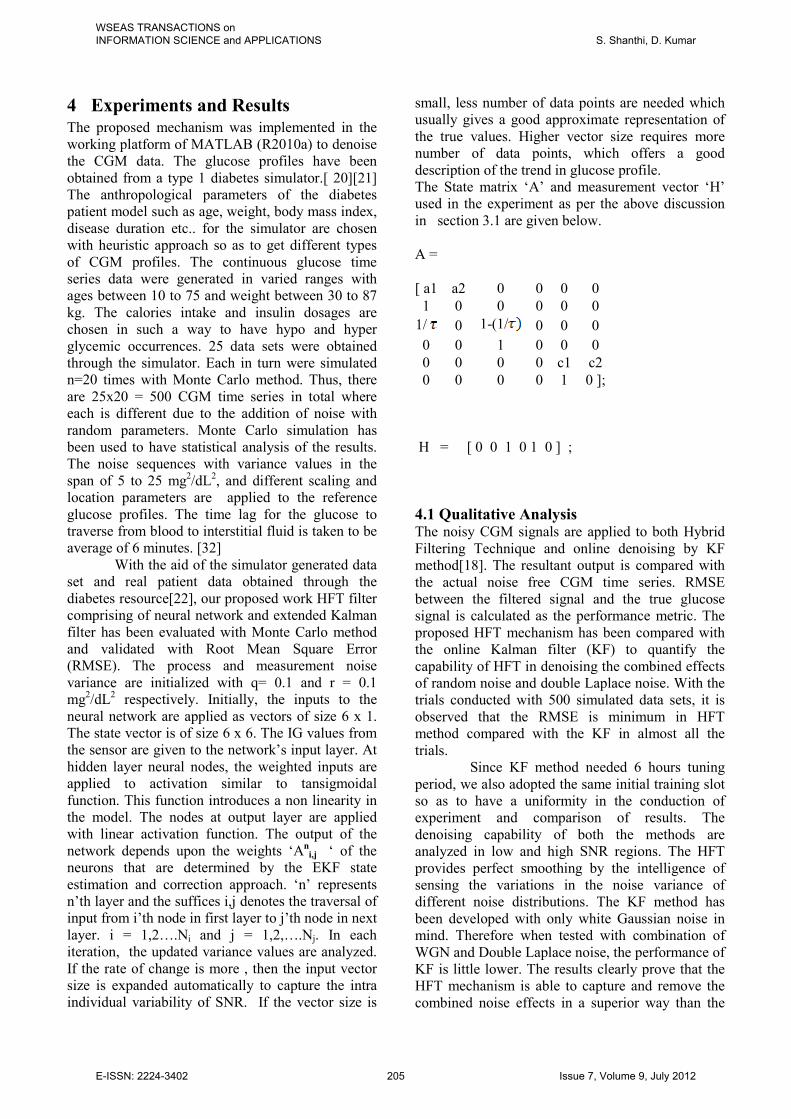
4 Experiments and Results The proposed mechanism was implemented in the

working platform of MATLAB (R2010a) to denoise

the CGM data. The glucose profiles have been

obtained from a type 1 diabetes simulator.[ 20][21]

The anthropological parameters of the diabetes

patient model such as age, weight, body mass index,

disease duration etc.. for the simulator are chosen

with heuristic approach so as to get different types

of CGM profiles. The continuous glucose time

series data were generated in varied ranges with

ages between 10 to 75 and weight between 30 to 87

kg. The calories intake and insulin dosages are

chosen in such a way to have hypo and hyper

glycemic occurrences. 25 data sets were obtained

through the simulator. Each in turn were simulated

n=20 times with Monte Carlo method. Thus, there

are 25x20 = 500 CGM time series in total where

each is different due to the addition of noise with

random parameters. Monte Carlo simulation has

been used to have statistical analysis of the results.

The noise sequences with variance values in the

span of 5 to 25 mg2/dL

2, and different scaling and

location parameters are applied to the reference

glucose profiles. The time lag for the glucose to

traverse from blood to interstitial fluid is taken to be

average of 6 minutes. [32]

With the aid of the simulator generated data

set and real patient data obtained through the

diabetes resource[22], our proposed work HFT filter

comprising of neural network and extended Kalman

filter has been evaluated with Monte Carlo method

and validated with Root Mean Square Error

(RMSE). The process and measurement noise

variance are initialized with q= 0.1 and r = 0.1

mg2/dL

2 respectively. Initially, the inputs to the

neural network are applied as vectors of size 6 x 1.

The state vector is of size 6 x 6. The IG values from

the sensor are given to the network’s input layer. At

hidden layer neural nodes, the weighted inputs are

applied to activation similar to tansigmoidal

function. This function introduces a non linearity in

the model. The nodes at output layer are applied

with linear activation function. The output of the

network depends upon the weights ‘Ani,j ‘ of the

neurons that are determined by the EKF state

estimation and correction approach. ‘n’ represents

n’th layer and the suffices i,j denotes the traversal of

input from i’th node in first layer to j’th node in next

layer. i = 1,2….Ni and j = 1,2,….Nj. In each

iteration, the updated variance values are analyzed.

If the rate of change is more , then the input vector

size is expanded automatically to capture the intra

individual variability of SNR. If the vector size is

small, less number of data points are needed which

usually gives a good approximate representation of

the true values. Higher vector size requires more

number of data points, which offers a good

description of the trend in glucose profile.

The State matrix ‘A’ and measurement vector ‘H’

used in the experiment as per the above discussion

in section 3.1 are given below.

A =

[ a1 a2 0 0 0 0

1 0 0 0 0 0

1/ 0 1-(1/ 0 0 0

0 0 1 0 0 0

0 0 0 0 c1 c2

0 0 0 0 1 0 ];

H = [ 0 0 1 0 1 0 ] ;

4.1 Qualitative Analysis The noisy CGM signals are applied to both Hybrid

Filtering Technique and online denoising by KF

method[18]. The resultant output is compared with

the actual noise free CGM time series. RMSE

between the filtered signal and the true glucose

signal is calculated as the performance metric. The

proposed HFT mechanism has been compared with

the online Kalman filter (KF) to quantify the

capability of HFT in denoising the combined effects

of random noise and double Laplace noise. With the

trials conducted with 500 simulated data sets, it is

observed that the RMSE is minimum in HFT

method compared with the KF in almost all the

trials.

Since KF method needed 6 hours tuning

period, we also adopted the same initial training slot

so as to have a uniformity in the conduction of

experiment and comparison of results. The

denoising capability of both the methods are

analyzed in low and high SNR regions. The HFT

provides perfect smoothing by the intelligence of

sensing the variations in the noise variance of

different noise distributions. The KF method has

been developed with only white Gaussian noise in

mind. Therefore when tested with combination of

WGN and Double Laplace noise, the performance of

KF is little lower. The results clearly prove that the

HFT mechanism is able to capture and remove the

combined noise effects in a superior way than the



other methods. This shows that the artificial neural

network in HFT is trained well with physiological

variations of each individual and it tracks the

glucose profile perfectly, neglecting the various

noise effects in the CGM time series. The denoising

effect of HFT in a representative noisy glucose

profile is shown in figure 8.

Fig : 8 Denoised CGM signal from HFT

The efficiency of HFT can very well be

observed with the comparison shown in figure 9.

Fig.9 Denoised CGM signal from KF , HFT

The smoothing performance of HFT is

corroborated with graphical representation of the

enlarged view of time frame of 16 to 19 hours in

figure 10 and time frame of 5 to 10 hours in figure

11 which are of different SNR values.

The figures clearly shows the

oscillations in noise variance in KF output when

compared with HFT which gives a smoother

output. This smoothness is due to the ability of

the artificial intelligent neural network that is

being trained with EKF algorithm in capturing

the non linear dynamics of the glucose profile.

Fig .10: Enlarged view of time frame 800-1200

minutes

Fig.11: Enlarged view of time frame 300-600

minutes

4.2 Quantitative Analysis The effect of denoising is quantitatively analyzed

with three indexes as in [18] i.e RMSE(calculated

between the denoised and real profile), the time

delay(calculated as the time shift which minimizes

the distance between true and denoised signal) and

SRG,the smoothness relative gain(calculated as the

normalized difference between energy of second

order differences of the original and denoised CGM

signals), in order to evaluate the regularity increase

of the denoised with respect to original CGM

profile. The RMSE obtained for HFT is with a mean

of 5.5 ± 1.6 and for KF it is 8.3 ± 2.6. The delay

introduced in the HFT is slightly higher ie. 1.9

minutes as an average whereas that of KF is 0.9

minutes. This delay is due to the estimation of

neural weights with respect to the varying noise



variances. SRG is high 0.95 thanks to the

intelligence of neural network. The experiments

were conducted with different scenarios and some

representative results are listed in table 1.

RMSE

(mg/dL)

Time Delay

(min)

SRG

S.

No

KF

HFT

KF

HFT

KF

HFT

1 6.1 4.3 0.42 0.54 0.88 0.91

2 4.3 2.5 0.11 0.19 0.89 0.92

3 7.8 5.1 0.22 0.35 0.76 0.89

4 9.4 3.9 0.18 0.31 0.65 0.95

5 10.9 6.1 0.90 1.53 0.5 0.99

6 5.7 3.3 0.23 1.15 0.74 0.89

7 3.8 1.0 0.15 0.39 0.56 0.88

8 8.1 4.2 0.75 1.21 0.81 0.95

9 7.3 5.7 0.80 0.91 0.69 0.88

10 6.7 3.0 0.75 0.89 0.78 0.90

11 5.9 4.1 0.67 0.71 0.67 0.89

12 8.6 5.2 0.33 0.42 0.61 0.87

13 9.3 5.5 0.15 0.71 0.74 0.91

14 10.5 6.1 0.19 0.65 0.59 0.87

15 9.0 5.7 0.32 0.43 0.74 0.99

Table 1: Performance Comparison of HFT and

Kalman Filter

5 Discussion Initially the approach of extended Kalman filter was

used by Knobbe and Buckingham for the estimation

of blood glucose and physiological parameters ( i.e

time lag ’t’ ) [12]. Their model includes five state

variables, each one has its own variance which have

to be trained. Whereas Fachinetti et al., focused on

EKF for improving the accuracy of CGM data by

enhanced calibration in cascade to the standard

device calibration. [17] Even though their model has

apparently six states, the true unknown variables are

only three. But different description of the

variables(i.e random walk process). Here in our

work we also adopted the random walk model

approach for BG and sensor gain deviation

parameter. The model order are fixed with Akaike

information criteria and the coefficients are arrived

with weighted least squares estimation. The

estimated state values and their variances are sent to

a neural network as parameters. The network is

trained initially with these values and are altered

gradually to meet out the required criteria of

minimum RMSE. This approach is a newer one

and we claim that the updation of neural weights

and biases by EKF procedure will perform good for

interindividual and intra individual variability of

SNR of CGM time series.

6 Conclusion The Continuous Glucose Monitoring is very much

essential for prevention of Diabetic complications.

Perfect filtering of various types of noise

distributions in CGM data enables it to be used for

further processing like Hypo/Hyper glycemic alert

generation and as control input to closed loop

artificial pancreas. Conventional filtering methods

are not sufficient to track the variations of

physiological signal neglecting the noise effects.

Our proposed work comprising the intelligent

artificial neural network with extended Kalman filter

algorithm has proved its success in denoising the

CGM signal with simulated data sets. The time lag

that occurs in the HFT due to enormous

computations of neural network can be nullified by

the latest high speed processors.

References:

[1] Jay S.Skyler ,”Continuous Glucose

Monitoring : An Overview of its

Development”, Diabetes Technology &

Therapeutics, vol. 11, sup.1,2009.

[2] B.Kovatchev, L.A.Gonder-Frederick, D.J.

Cox, W.L.Clarke, “ Evaluating the

accuracy of Continuous glucose

monitoring sensors: continuous glucose-



error grid analysis illustrated by

TheraSenseFreestyle Navigator data”,

Diabetes Care, 2004 Aug;27(8); 1922-

1928.

[3] B.Kovatchev, S.Anderson, L.Heinemann,

and W.L.Clarke,”Comparison of the

numerical and Clinical accuracy of four

continuous glucose monitors,” Diabetes

Care, vol.31,pp.1160-1164,2008.

[4] Klonoff D, Bernhardt P, Ginsberg BH,

Joseph J, Mastrototaro J, Parker DR,

Vesper H, Vigersky R.CLSI document

POCT05-A (ISBN 1-56238-685-9)

Clinical and Laboratory Standards

Institute; 2008.Performance metrics for

continuous interstitial glucose monitoring;

approved guideline.

[5] Mastrototaro JJ, Gross TM, Shin JJ.

Glucose monitor calibration methods.

United States patent US 6,424,847. 2002

Jul 23.

[6] Steil G, Rebrin K. Closed-loop system for

controlling insulin infusion. United States

patent US 7,354,420 B2. 2008 Apr 8;

[7] Gross TM, Bode BW, Einhorn D, Kayne

DM, Reed JH, White NH, Mastrototaro

JJ: Performance evaluation of the

MiniMed continuous glucose monitoring

system during patient home use.

Diabetes Technol Ther 2:49–56, 2000.

[8] Goode PV, Jr, Brauker JH, Kamath AU.

System and methods for processing

analyte sensor data. United States

patent US 6,931,327 B2. 2005 Aug 16;

[9] Panteleon A, Rebrin K, Steil GM. The role

of the independent variable to glucose

sensor calibration. Diabetes Technol Ther.

2003;5(3):401–410.

[10] Keenan DB, Mastrototaro JJ, Voskanyan

G, Steil GM. Delays in minimally

invasive Continuous glucose monitoring

devices: a review of current technology. J

Diabetes Science Technology

009;3(5):1207–1214.

[11] J. G. Chase, C. E. Hann, M. Jackson, J.

Lin, T. Lotz, X. W. Wong, and G. M.

Shaw, “Integral-based filtering of

continuous glucose sensor measurements

for glycemic control in critical care,”

Comput. Methods Programs Biomed.,

vol. 82, pp. 238–247, 2006.

[12] Knobbe, E.J.; Bucking.B.,”the extended

Kalman for continuous glucose

monitoring”, Diabetes TechnolTher 7:15

–27, 2005.

[13] Palerm CC, Willis JP, Desemone J,

Bequette BW. Hypoglycemia prediction

and detection using optimal estimation.

Diabetes Technol Ther. 2005;7(1):3–14.

[14] Palerm CC, Bequette BW. Hypoglycemia

detection and prediction using continuous

glucose monitoring–a study on

hypoglycemic clamp data. J Diabetes Sci

Technol. 2007;1(5):624–629.

[15] Kuure-Kinsey M, Palerm CC, Bequette

BW. A dual-rate Kalman filter for

continuous glucose monitoring. Proc.

IEEE EMB Conference; 2006. pp. 63–66.

[16] Facchinetti, G. Sparacino and Claudio

Cobelli, “An Online Self-Tunable Method

to Denoise CGM Sensor Data “ IEEE

Trans.on Bio.Med Engg, vol. 57, no. 3,

March 2010


Cobelli,“Enhanced Accuracy of

Continuous Glucose Monitoring by

Online Extended Kalman Filtering,”

Diabetes Technol Ther ,vol.12, No 5,2010


Cobelli, “Online Denoising Method to

Handle Intraindividual Variability of

Signal-to-Noise Ratio in Continuous

Glucose Monitoring“ IEEE Trans.on

Bio.Med Engg, vol. 58, no. 9, September

2011.

[19] Xuesong Chen, “ Impact of Continuous

Glucose Monitoring System on Model

Based Glucose Control” PhD Thesis,

University of Canterbury, Christchurch,

New Zealand, May 2007.

[20] Dalla Man C, Raimondo DM, Rizza RA,

Cobelli C: GIM, simulation software of meal

glucose-insulin model. J Diabetes Sci

Technol 2007;1:323–330.

[21] Dalla Man C, Rizza RA, Cobelli C: Meal

simulation model of the glucose-insulin

system. IEEE Trans Biomed Eng 2007;54:

1740–1749.

[22] http://glucosecontrol.ucsd.edu(accessed

January 4, 2012).

[23] The Laplace distribution and generalizations:

a revisit with applications to

Communications, Economics,Engineering

and Finance, Samuel Kotz,Tomasz J.

Kozubowski, Krzysztof Podgórski,

Birkhauser Publications, Boston, 2001.

[24] Breton M, Kovatchev BP: Analysis,

modeling, and simulation of the accuracy of

continuous glucose sensors. J Diabetes Sci

Technol 2008;2:853–862.



[25] Giovanni Sparacino, Andrea Facchinetti and

Claudio Cobelli,” “Smart” Continuous

Glucose Monitoring Sensors: On-Line

Signal Processing Issues”, Sensors, Vol.10,

No.7, pp.6751-6772, July 2010

[26] P.Goldberg, M.S., R Russell, R.Sherwin,

R.Halickman, J.Cooper, D.Dziura ans

S.Nzucchi , “Experience with continuous

glucose monitoring system in a medical

intensive care unit.” Diabetes Technol.

Therapeutics, 6(3), 2004 pp 339-347.

[27] Eda Cengiz and William V. Tamborlane , A

Tale of Two Compartments: Interstitial

Versus Blood Glucose Monitoring. Diabetes

Technol Ther ,vol.11, sup.1,2009

[28] Brockwell, P.J., and Davis, R.A.

(2009). Time Series: Theory and Methods,

2nd ed. Springer.

[29] Julier,S.J.; Uhlmann,J.K; “ Unscented

filtering and non linear estimation”,

Proceedings of the IEEE, March

2004,pg:401-422.

[30] Phee,H.K, Tung,W.L & Quek,C, A

Personalized approach to insulin regulation

using brain-inspired neural semantic

memory in diabetic glucose control. IEEE

congressOnEvolutionaryComputation,2007,

Singapore,pp.2644-2651.

[31] V.Tresp, T.Briegel, and J.Moody, ”Neural-

network models for the blood glucose

metabolism for a diabetic,” IEEE Transactions

on Neural networks,vol.10,pp. 104-1213,1999.

[32] Gayane Voskanyan,Barry Keenan, John

J.Mastrototaro and Garry M.Steil, Putative

delays in Interstitial Fluid (ISF) Glucose

Kinetics Can be attributed to the Glucose

Sensing systems Used to Measure them

Rather Than the Delay in ISF Glucose Itself.

Journal of Diabetes Science and

Technology, vol.1,issue 5, Sep 2007.

[33] Zarita Zainuddin, Ong Pauline and Cemal

Ardil,“A neural network approach in

Predicting the Blood Glucose Level for

Diabetic Patients”, International Journal of

Computational Intelligence 5:1,2009.

[34] Shanthi S, Kumar Durai, “Continuous

Glucose Monitoring Sensor Data: Denoising

with Hybrid of Neural Network and

Extended Kalman Filter Algorithm”,

European Journal of Scientific Research,

Vol.66, No.2,2011,pp.293-302.



Neural Network Based Filter for Continuous Glucose ... · Neural Network Based Filter for...

Documents

Transcript of Neural Network Based Filter for Continuous Glucose ... · Neural Network Based Filter for...