Monitoring Network Traffic with Radial Traffic Analyzer - CiteSeer

1Traffic
Network Traffic #6
Victor S. FrostDan F. Servey Distinguished Professor
Electrical Engineering and Computer ScienceUniversity of Kansas2335 Irving Hill Dr.
Lawrence, Kansas 66045Phone: (785) 864-4833 FAX:(785) 864-7789
e-mail: [email protected]://www.ittc.ku.edu/
Section 4.7.1, 5.7.2
2Traffic
Traffic CharacterizationGoals to:
Understand the nature of what is transported over communications networks. Use understanding to improve network design
Traffic Characterization describes the user demands for network resources
How often a customer:– Requests a web page– Down loads an MP3– Makes a phone call
Size/length – Web page– Song– Phone call

3Traffic
Voice Traffic: Aggregate Traffic
Requests for network resources from a large population of users.
Large Populationof Users System
SwitchingSystem
***
1
M
***1 N
Large Populationof Users
4Traffic
Voice Traffic:Aggregate Traffic
Arrival RateNumber of requests/time unit
– Calls/sec
Holding Time, length of time the request will use the network resources
Min./callsec/packet
Arrival rate = λ
Average Holding Time =hT

5Traffic
Voice Traffic:Aggregate Traffic
Traffic Intensity (load)Product of the average holding time and the arrival rate
Units of Traffic IntensityErlangsCCS [1 CCS is 100 call sec/hr ]1 Erlang = 36 CCS
Traffic intensity is specified for the 'Busy Hour'
hT Intensity Traffic λρ ==
6Traffic
Voice Traffic:Aggregate Traffic
A telephone line busy 100% of the time= 1 Erlang
A telephone busy 6 min/hour is how much traffic
0.1 Erlang100 telephones busy 10% of the time is how much traffic10 Erlangs

7Traffic
Voice Traffic:Aggregate Traffic
A telephone busy 100 sec (Centi call Seconds, CCS) per hour = 1
CCSArrival rate = 1 call/hourAverage holding time = 100 secSo
(100 sec/call)*(1 hour/3600sec)*(1call/hour) = 1/36 Erlangs
= 1 CCS36 CCS = 1 Erlang
8Traffic
Voice Traffic:Aggregate Traffic
Traffic is RandomHolding timeInterarrival time (time between calls)
Common assumptions for probability density function (pdf) for
Holding time ~ exponentialInterarrival time ~ exponential
Section 4.7.1 and A.1.1
9Traffic
Voice Traffic:Aggregate Traffic
Interarrival Histogram
10Traffic
Voice Traffic:Aggregate Traffic
P [ Th< t ] = 1 - e - µ t for t > 0 and 0 for t < 0
T h =1
µ
P [T I < t ] = 1 - e -λ t for t > 0 and 0 for t < 0
T I = Interarrival time

11Traffic
Voice Traffic:Aggregate Traffic
Time
TI
Time
Th
12Traffic
Voice Traffic:Aggregate Traffic-Diurnal Variation
13Traffic
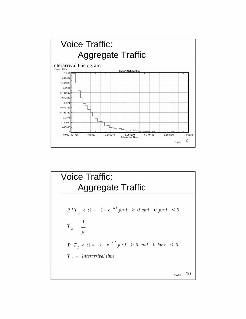
Voice Traffic: Individual voice source
Speech inactivity factor
time
Talkspurt Talkspurt Talkspurt
SilenceSilence
14Traffic
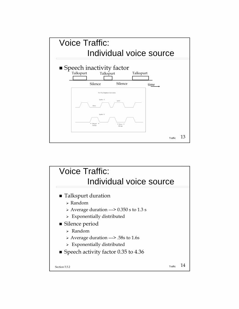
Voice Traffic: Individual voice source
Talkspurt durationRandomAverage duration ---> 0.350 s to 1.3 sExponentially distributed
Silence period RandomAverage duration ---> .58s to 1.6sExponentially distributed
Speech activity factor 0.35 to 4.36
Section 5.5.2
15Traffic
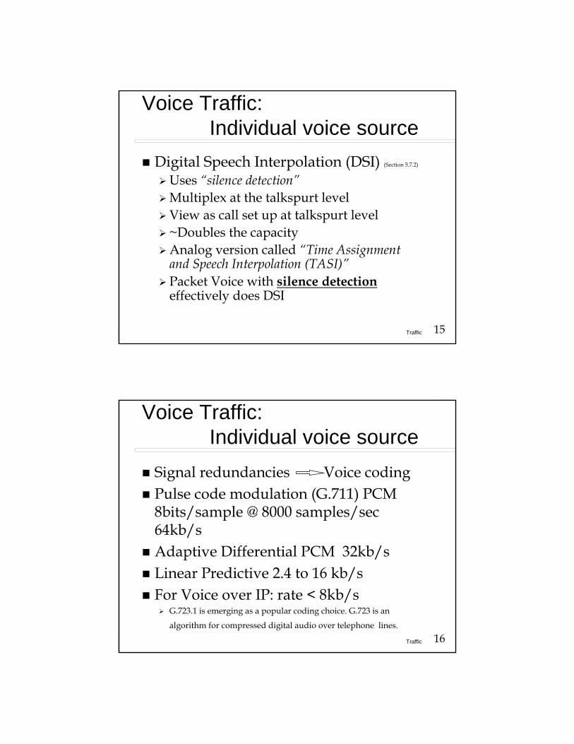
Voice Traffic: Individual voice source
Digital Speech Interpolation (DSI) (Section 5.7.2)
Uses “silence detection” Multiplex at the talkspurt levelView as call set up at talkspurt level~Doubles the capacityAnalog version called “Time Assignment and Speech Interpolation (TASI)”Packet Voice with silence detectioneffectively does DSI
16Traffic
Voice Traffic: Individual voice source
Signal redundancies Voice codingPulse code modulation (G.711) PCM 8bits/sample @ 8000 samples/sec 64kb/sAdaptive Differential PCM 32kb/sLinear Predictive 2.4 to 16 kb/sFor Voice over IP: rate < 8kb/s
G.723.1 is emerging as a popular coding choice. G.723 is an
algorithm for compressed digital audio over telephone lines.

17Traffic
Comparison of popular CODECs
LowGoodHigh8G.729 CS-ACELP
LowGoodVery high16G.728 LD-CELP
Very lowGood (40)Fair (24)
Low40/32/24G.726 ADPCM
HighGood (6.4)Fair (5.3)
Moderate 6.4/5.3G.723 MP-MLQ
N/AExcellentNot required64 (no compression)G.711 PCM
Added delayResultant voice quality
Required CPU resources
Compressed rate (Kbps)
Compression scheme
There is no "right CODEC". The choice of what compression scheme to use depends on what parameters aremore important for a specific installation.
In practice, G.723 and G.729 are more popular that G.726 and G.728.
For details of other VoIP Codecs see:http://www.zytrax.com/tech/protocols/voip_rates.htm
18Traffic
Voice Traffic: Individual voice source
Example: How many calls can be supported on a system with the following parameters?
TDMCoding rate/voice channel = ADPCMDSI Line rate = 1.536 Mb/s
(note a T1/DS1 line is 1.544 Mb/s)
Number of ADPCM channels = (1.563 Mb/s)/(32 Kb/s) = 48
With DSI you get 2 calls/channel = 96
19Traffic
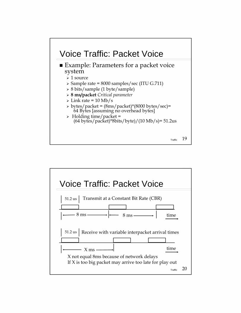
Voice Traffic: Packet VoiceExample: Parameters for a packet voice system
1 sourceSample rate = 8000 samples/sec (ITU G.711)8 bits/sample (1 byte/sample)8 ms/packet Critical parameterLink rate = 10 Mb/sbytes/packet = (8ms/packet)*(8000 bytes/sec)=
64 Bytes [assuming no overhead bytes]Holding time/packet = (64 bytes/packet)*8bits/byte)/(10 Mb/s)= 51.2us
20Traffic
Voice Traffic: Packet Voice51.2 us
8 ms time
51.2 us
X ms time
8 ms
Transmit at a Constant Bit Rate (CBR)
X not equal 8ms because of network delaysIf X is too big packet may arrive too late for play out
Receive with variable interpacket arrival times

21Traffic
Voice Traffic: Packet Voice
51.2 us
8 ms time
1 2 N 1
Perfect Multiplexing of N VoIP sources
22Traffic
Voice Traffic: Packet VoicePacket voice looks like a steady flow or Constant Bit Rate (CBR) trafficHowever, voice can be Variable Bit Rate or VBR
“silence detection”Variable rate coding
Problem: After going through the network the packets will not arrive equally spaced in time. Thus playback of packet voice must deal with variable network delays
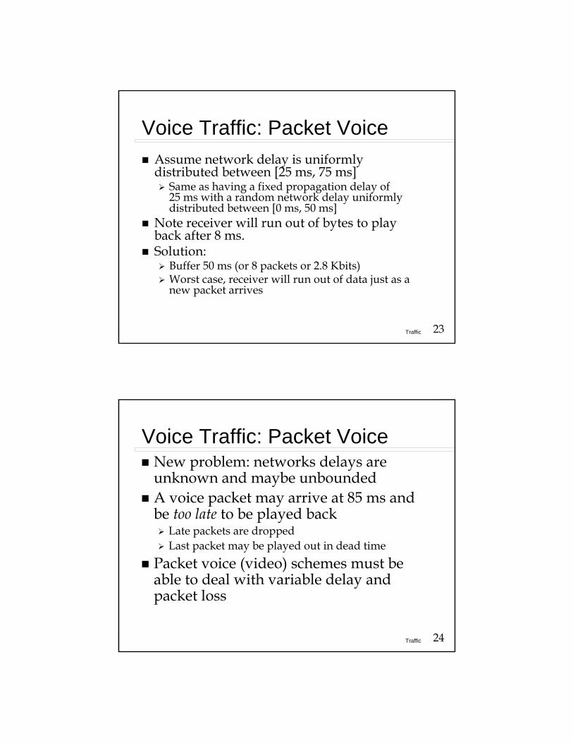
23Traffic
Voice Traffic: Packet VoiceAssume network delay is uniformly distributed between [25 ms, 75 ms]
Same as having a fixed propagation delay of 25 ms with a random network delay uniformly distributed between [0 ms, 50 ms]
Note receiver will run out of bytes to play back after 8 ms.Solution:
Buffer 50 ms (or 8 packets or 2.8 Kbits)Worst case, receiver will run out of data just as a new packet arrives
24Traffic
Voice Traffic: Packet VoiceNew problem: networks delays are unknown and maybe unboundedA voice packet may arrive at 85 ms and be too late to be played back
Late packets are droppedLast packet may be played out in dead time
Packet voice (video) schemes must be able to deal with variable delay and packet loss
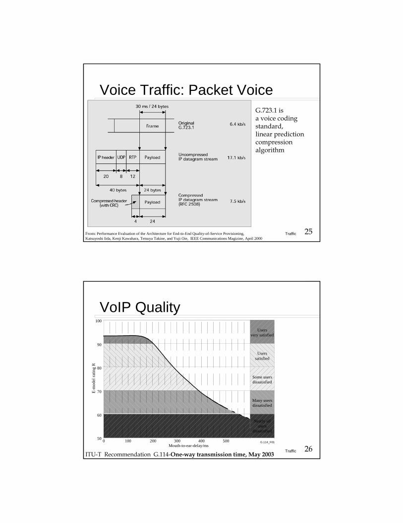
25Traffic
Voice Traffic: Packet VoiceG.723.1 is a voice codingstandard, linear predictioncompressionalgorithm
From: Performance Evaluation of the Architecture for End-to-End Quality-of-Service Provisioning,Katsuyoshi Iida, Kenji Kawahara, Tetsuya Takine, and Yuji Oie, IEEE Communications Magizine, April 2000
26Traffic
VoIP Quality
G.114_F010 100 200 300 400 50050
60
70
80
90
100
Nearly allusers
dissatisfied
Many usersdissatisfied
Some usersdissatisfied
Userssatisfied
Usersvery satisfied
Mouth-to-ear-delay/ms
E-m
odel
ratin
g R
ITU-T Recommendation G.114-One-way transmission time, May 2003
27Traffic
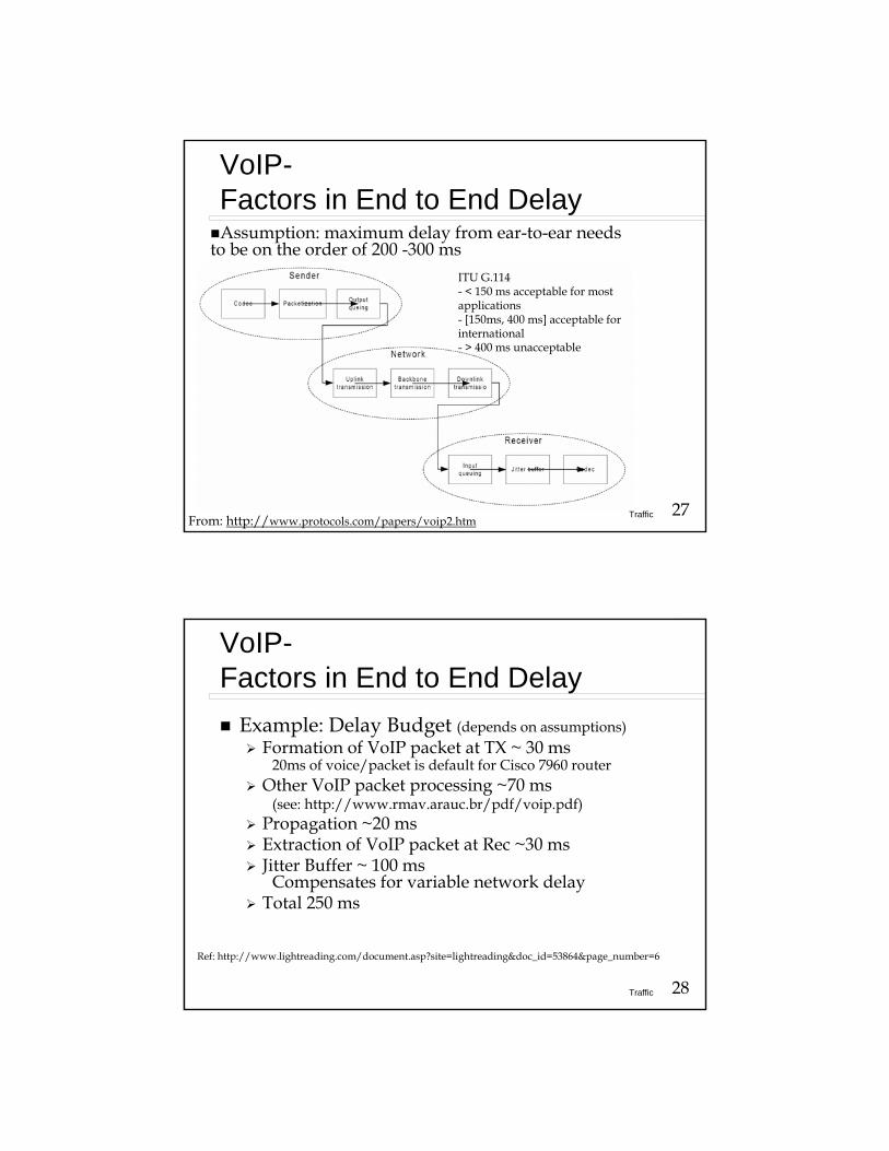
VoIP-Factors in End to End DelayAssumption: maximum delay from ear-to-ear needs
to be on the order of 200 -300 ms
From: http://www.protocols.com/papers/voip2.htm
ITU G.114 - < 150 ms acceptable for most applications- [150ms, 400 ms] acceptable for international- > 400 ms unacceptable
28Traffic
VoIP-Factors in End to End Delay
Example: Delay Budget (depends on assumptions)Formation of VoIP packet at TX ~ 30 ms
20ms of voice/packet is default for Cisco 7960 routerOther VoIP packet processing ~70 ms
(see: http://www.rmav.arauc.br/pdf/voip.pdf)Propagation ~20 msExtraction of VoIP packet at Rec ~30 msJitter Buffer ~ 100 ms
Compensates for variable network delayTotal 250 ms
Ref: http://www.lightreading.com/document.asp?site=lightreading&doc_id=53864&page_number=6

29Traffic
Data Traffic: General Characteristics
Highly variableNot well knownLikely to change as new services and applications evolve.
30Traffic
Data Traffic: General Characteristics
Highly bursty, where one definition of burstyness is:
Burstyness = Peak rateAverage rate

31Traffic
Data Traffic: General Characteristics
Example: During a typical remote login connectionover a 19.2kb/s modem a user types at a rate of 1 symbol/sec or 8 bits/sec and then transfers a 100 kbyte file. Assume the total holding time of the connection is 10 min.
What is the burstyness of this data session?
32Traffic
Data Traffic: General Characteristics
The time to transfer the file is (800,000 bits)/(19,200 b/s) = 41 sec.So for 600 - 41sec = 559 sec. the data rate is 8 bits/sec or 4,472 bits were transferred in 559 sec. Thus in 600 sec. 4,472 + 800,000 bits were transferred, yielding a average rate of:804,472 bits/600 sec = 1,340 bits/sec.The peak rate was 19.2 Kb/s so the burstyness for this data session was:
19,200/1,340 = 14.3

33Traffic
Data Traffic: General Characteristics
Session Interarrivals
Session Duration
Packet Interarrivals
Packet Lengths
CallArrival
CallDuration
VoIPPacket Arrivals
VoIPPacket Lengths
34Traffic
Data Traffic: General Characteristics
User Burst
Idle TimeComputer Burst
Think Time
User Burst
Idle TimeComputer Burst
Asymmetric Nature of Interactive Traffic
This Asymmetric property has lead to asymmetric services

35Traffic
Data Traffic: General Characteristics
In Time Division Multiplexing (TDM) user must wait for turn to use link. Statistical Multiplexing (Stat Mux)
Note high burstness leads to “long” idle timesBy transmitting the ‘bursts’ on demand the link can be efficiently shared.To help insure fairness break the ‘burst’into packets and transmit on a packet basis
36Traffic
TDM vs Stat Mux
Server
Dwell time = one time slotUser 1
User N
Server
User 1
User N

37Traffic
Data Traffic: General Characteristics
Element lengthMessagePacketCell
Arrival rateMessage/secPackets/secCells/sec
38Traffic
Data Traffic: General Characteristics
Traffic intensity (< 1 with one server)ρ = λ T
h
where
T h=
Average Packet Length in Bits
Link Capacity in Bits / sec=
L
C
Average Packet Length in Bits = L
Link Capacity in Bits / Sec = C
39Traffic
Data Traffic: General Characteristics
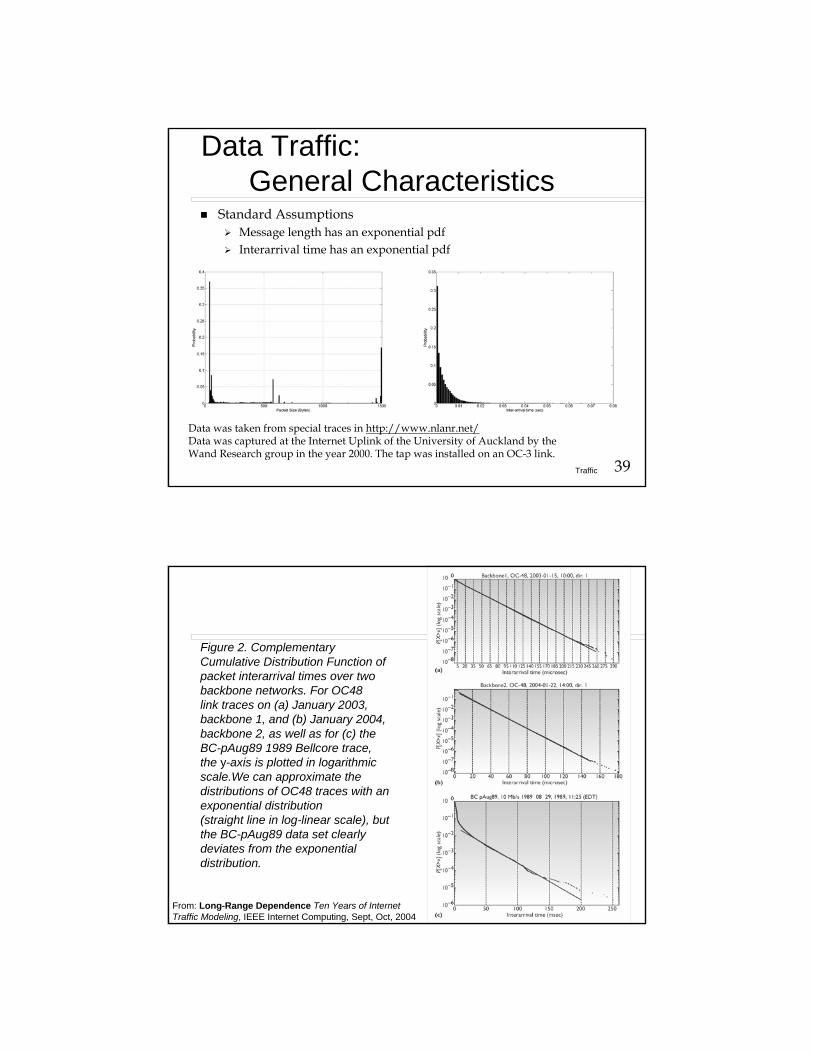
Standard AssumptionsMessage length has an exponential pdfInterarrival time has an exponential pdf
Data was taken from special traces in http://www.nlanr.net/Data was captured at the Internet Uplink of the University of Auckland by the Wand Research group in the year 2000. The tap was installed on an OC-3 link.
40TrafficFrom: Long-Range Dependence Ten Years of Internet Traffic Modeling, IEEE Internet Computing, Sept, Oct, 2004
Figure 2. Complementary Cumulative Distribution Function ofpacket interarrival times over two backbone networks. For OC48link traces on (a) January 2003, backbone 1, and (b) January 2004,backbone 2, as well as for (c) the BC-pAug89 1989 Bellcore trace,the y-axis is plotted in logarithmic scale.We can approximate thedistributions of OC48 traces with an exponential distribution(straight line in log-linear scale), but the BC-pAug89 data set clearlydeviates from the exponential distribution.
41Traffic
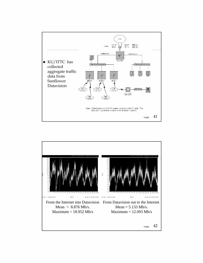
KU/ITTC has collected aggregate traffic data from Sunflower Datavision
42Traffic
From the Internet into DatavisionMean = 8.876 Mb/s.
Maximum = 18.952 Mb/s
From Datavision out to the Internet Mean = 5.133 Mb/s.
Maximum = 12.093 Mb/s
43Traffic
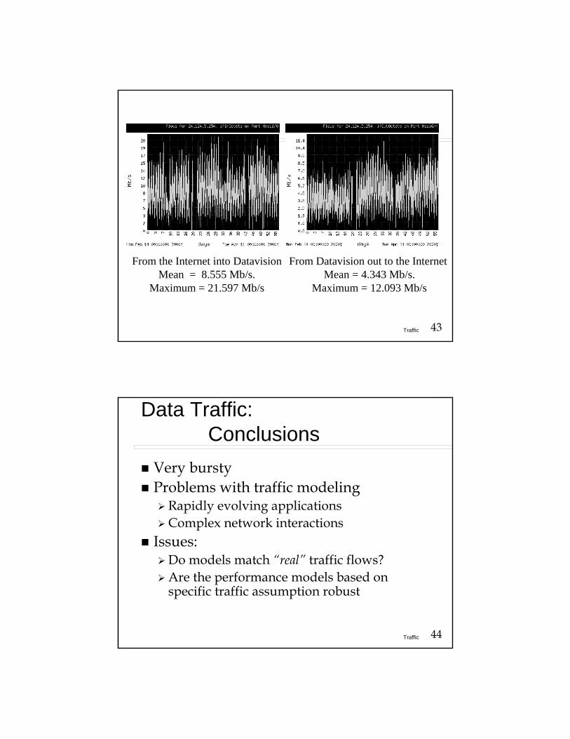
From the Internet into DatavisionMean = 8.555 Mb/s.
Maximum = 21.597 Mb/s
From Datavision out to the Internet Mean = 4.343 Mb/s.
Maximum = 12.093 Mb/s
44Traffic
Data Traffic: Conclusions
Very burstyProblems with traffic modeling
Rapidly evolving applicationsComplex network interactions
Issues:Do models match “real” traffic flows?Are the performance models based on specific traffic assumption robust
45Traffic
Video: Analog video
Bandwidth ~ 4 MhzUncompressed rate 64 Mb/sComponents of the signal
LuminanceChrominanceAudioSynchronization
46Traffic
Digital Video: JPEG"Joint Photographic Expert Group". Voted as international standard in 1992. Suitable for color and grayscale images, e.g., satellite, medical applications.Targeted for still imagesCapable of reducing continuous true color or gray-scale images to less than 5% of their original sizeJPEG (GIF and MPEG) define the compression as well as the video data format
Section 12.3
47Traffic
Digital Video: MPEGMoving Pictures Experts GroupCompresses moving pictures taking advantage of frame-to-frame redundanciesMPEG Initial Target: VHS quality on a CD-ROM (320 x 240 + CD audio @ 1.5 Mbits/sec)
48Traffic
Digital Video: MPEGConverts a sequence of frames into a compressed format of three frame typesI Frames (intrapicture)P frames (predicted picture)B frames (bidirectional predicted picture)
49Traffic
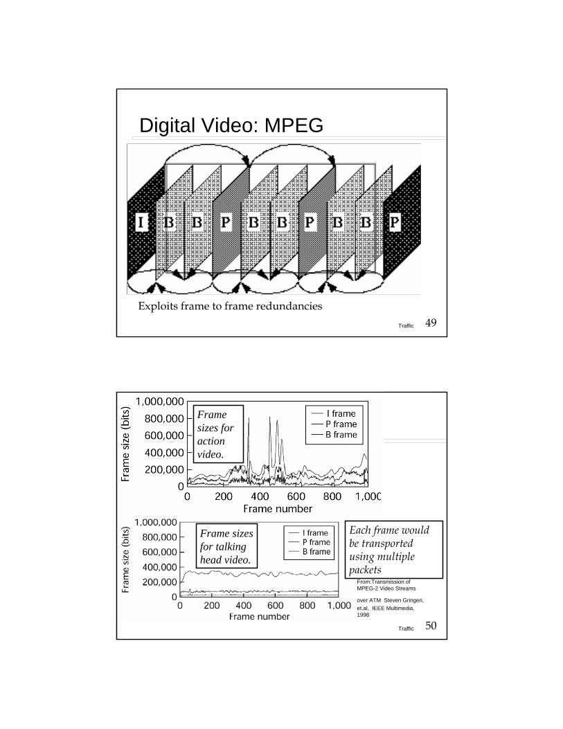
Digital Video: MPEG
Exploits frame to frame redundancies
50Traffic
Frame sizesfor talking head video.
Frame sizes foraction video.
From:Transmission of MPEG-2 Video Streams
over ATM Steven Gringeri, et.al, IEEE Multimedia, 1998
Each frame would be transported using multiple packets

51Traffic
MP3- MPEG Layer 3 AudioMPEG specifies a family of three audio coding schemes, Layer-1,-2,-3, Each Layer has and increasing encoder complexity and performance(sound quality per bitrate) The three codecs are compatible in a hierarchical way, i.e. a Layer-N decoder is able to decode bit stream data encoded in Layer-N and all Layers below NThe MP3 compression algorithm is based on a complicated psycho-acoustic modelThe majority of the files available on the Internet are encoded in 128 kbits/s stereo. A high quality file is 12 times smaller than the original CDs can be created that contain over 160 songs and can play for over 14 hours on a PC.Music can be efficiently stored on a hard disk and then directly played
from there
52Traffic
Digital Video: MPEGCompression ranges:
30-to150-to-1
MPEG is evolvingMPEG 1MPEG 2MPEG 4MPEG 7
53Traffic
Digital Video: MPEG-4
Audio-video coding for “low bit-rate”channels,
InternetMobile applications
MPEG-4 is a significant change from MPEG-2Scalability is a key feature of MPEG-4MPEG-4 contains a Intellectual Property rights (IPR) management infrastructure
54Traffic
Digital Video: MPEG-4Object based: Audio-visual objects (AVO)AVO are described mathematically and given a position in 2D or 3D spaceViewer can change vantage point and update calculations done locallyNo distinction between “natural” and “synthetic” AVOs: treats two in an integrated fashionEach AVO is represented separately and becomes the basis for an independent streamEach AVO is reusable, with the capability to incorporate on-the-fly elements under application controlContent transport with QoS for each component

55Traffic
ConclusionsNetwork traffic defines the demands for network resourcesNetwork traffic is dynamic
Changes with the deployment of new applicationTime of day
Models for network traffic are continuing to evolve