Rumors, consensus and epidemics on networks A.J. Ganesh University of Bristol.

University of CaliforniaSanta Barbara
Network systems: Social networks, Epidemics,
Optimization and Contraction Theory
A dissertation submitted in partial satisfaction
of the requirements for the degree
Doctor of Philosophy
in
Electrical and Computer Engineering
by
Pedro A. Cisneros
Committee in charge:
Professor Francesco Bullo, ChairProfessor Ambuj SinghProfessor Jason MardenProfessor Joao Hespanha
June 2021
The dissertation of Pedro A. Cisneros is approved.
Professor Ambuj Singh
Professor Jason Marden
Professor Joao Hespanha
Professor Francesco Bullo, Committee Chair
April 2021

Network systems: Social networks, Epidemics, Optimization and Contraction Theory
Copyright c© 2021
by
Pedro A. Cisneros
iii

Para mi familia: Pedro, Lourdes, Sergio y abuelos.
iv

Acknowledgements
I am deeply grateful to Prof. Francesco Bullo, my advisor, for all the help and good ad-
vising during my PhD studies. Without him, this accomplishment could not be possible.
I am also grateful to my family for their unconditional support, especially my parents and
brother. I am also grateful to my friend Mary. I am also grateful to all the professors,
students and collaborators whose interactions and help have been very helpful during my
studies, with a special mention to Dr. Saber Jafarpour, Prof. Ambuj Singh, and Prof.
Alex Petersen. For the funding, I am also grateful for the support from the ARO MURI
project, grant number W911NF-15-1-0577
I am grateful to God for all the blessings throughout my studies. Gloria in excelsis
Deo, in saecula saeculorum.
v

Curriculum VitæPedro A. Cisneros
Education
2021 Ph.D. in Electrical and Computer Engineering, University of Cali-fornia, Santa Barbara.
2020 M.A. in Mathematical Statistics, University of California, SantaBarbara.
2018 M.S. in Electrical and Computer Engineering, University of Cali-fornia, Santa Barbara.
Published and submitted work:
P. Cisneros-Velarde, K Chan, F Bullo. ”Polarization and fluctuations in signed socialnetworks.” IEEE Transactions on Automatic Control. 2020.P. Cisneros-Velarde, N.E. Friedkin, A.V. Proskurnikov, F. Bullo. ”Structural Balancevia Gradient Flows over Signed Graphs.” IEEE Transactions on Automatic Con-trol. 2020.P. Cisneros-Velarde, A. Petersen, S.Y. Oh. ”Distributionally Robust Formulation andModel Selection for the Graphical Lasso.” AISTATS, 2020.P. Cisneros-Velarde, F. Bullo. ”Signed Network Formation Games and ClusteringBalance.” Dynamic Games and Applications. 2020.P. Cisneros-Velarde, F. Bullo. ”Distributed Wasserstein Barycenters via DisplacementInterpolation.” Preprint. 2020.P. Cisneros-Velarde, S. Jafarpour, F Bullo. ”Contraction Theory for Dynamical Sys-tems on Hilbert Spaces.” Preprint. 2020.P. Cisneros-Velarde, F Bullo. ”Multi-group SIS Epidemics with Simplicial and Higher-Order Interactions.” Preprint. 2020.P. Cisneros-Velarde, S Jafarpour, F Bullo. ”Distributed and time-varying primal-dualdynamics via contraction analysis.” Preprint. 2020.P. Cisneros-Velarde, F Bullo. ”A Network Formation Game for the Emergence ofHierarchies.” Preprint. 2020.S. Jafarpour, P. Cisneros-Velarde, F Bullo. ”Weak and Semi-Contraction Theory withApplication to Network Systems.” IEEE Transactions on Automatic Control. 2021W. Mei, P. Cisneros-Velarde, G. Chen, N.E. Friedkin, F. Bullo. ”Dynamic social bal-ance and convergent appraisals via homophily and influence mechanisms.” Automatica.2019.
vi

Abstract
Network systems: Social networks, Epidemics, Optimization and Contraction Theory
by
Pedro A. Cisneros
In this thesis, I will first present mathematical models that explain the evolution of in-
terpersonal relationships in a social network, represented by a signed graph, converging
to structures that have a long history in sociology - namely, structural and clustering
balance. Then, I will present a simple model for the evolution of opinions over signed
graphs, including the aforementioned special structures. Then, I will present an im-
portant phenomenon that occurs on the susceptible-infected-susceptible (SIS) model of
epidemics: the emergence of a new epidemic domain of bistability when higher-order in-
teraction among individuals are considered on the contact network. Then, I will present
an algorithm for the computation of Wasserstein barycenters, and show a connection
with the theory of opinion dynamics. Finally, the last part of this thesis is devoted to the
study and application of contraction theory, an important tool that certifies incremental
stability. We study its expansion to dynamical systems on Hilbert spaces, as well as its
application to various optimization problems and settings.
vii

Contents
Curriculum Vitae vi
Abstract vii
1 Structural Balance via Gradient Flows over Signed Graphs 11.1 Introduction . . . . . . . . . . . . . . . . . . . . . . . . . . . . . . . . . . 11.2 Preliminaries . . . . . . . . . . . . . . . . . . . . . . . . . . . . . . . . . 61.3 Proposed models and representation as gradient flows . . . . . . . . . . . 101.4 Classification of symmetric equilibria . . . . . . . . . . . . . . . . . . . . 181.5 Convergence to balanced equilibria and stability analysis . . . . . . . . . 291.6 Simulation results and conjectures . . . . . . . . . . . . . . . . . . . . . . 341.7 Conclusion . . . . . . . . . . . . . . . . . . . . . . . . . . . . . . . . . . . 381.8 Appendix . . . . . . . . . . . . . . . . . . . . . . . . . . . . . . . . . . . 39
2 Polarization and Fluctuations in Signed Social Networks 462.1 Introduction . . . . . . . . . . . . . . . . . . . . . . . . . . . . . . . . . . 462.2 The model . . . . . . . . . . . . . . . . . . . . . . . . . . . . . . . . . . . 492.3 Model analysis . . . . . . . . . . . . . . . . . . . . . . . . . . . . . . . . 532.4 Conclusion . . . . . . . . . . . . . . . . . . . . . . . . . . . . . . . . . . . 602.5 Appendix . . . . . . . . . . . . . . . . . . . . . . . . . . . . . . . . . . . 60
3 Multi-group SIS Epidemics with Simplicial and Higher-Order Interac-tions 633.1 Introduction . . . . . . . . . . . . . . . . . . . . . . . . . . . . . . . . . . 633.2 Preliminaries and notation . . . . . . . . . . . . . . . . . . . . . . . . . . 693.3 Exponential convergence and matrix measures . . . . . . . . . . . . . . . 713.4 The Simplicial SIS model . . . . . . . . . . . . . . . . . . . . . . . . . . . 723.5 Analysis of the model . . . . . . . . . . . . . . . . . . . . . . . . . . . . . 753.6 Analysis of higher-order models . . . . . . . . . . . . . . . . . . . . . . . 893.7 Numerical example . . . . . . . . . . . . . . . . . . . . . . . . . . . . . . 913.8 Conclusion . . . . . . . . . . . . . . . . . . . . . . . . . . . . . . . . . . . 92
viii

4 Distributed Wasserstein Barycenters via Displacement Interpolation 954.1 Introduction . . . . . . . . . . . . . . . . . . . . . . . . . . . . . . . . . . 954.2 Notation and preliminary concepts . . . . . . . . . . . . . . . . . . . . . 1014.3 Proposed algorithm and analysis . . . . . . . . . . . . . . . . . . . . . . . 1044.4 Proofs of results in Section 4.3 . . . . . . . . . . . . . . . . . . . . . . . . 1154.5 The relevance of the PaWBar algorithm in opinion dynamics . . . . . . . 1334.6 Conclusion . . . . . . . . . . . . . . . . . . . . . . . . . . . . . . . . . . . 135
5 Contraction Theory for Dynamical Systems on Hilbert Spaces 1365.1 Introduction . . . . . . . . . . . . . . . . . . . . . . . . . . . . . . . . . . 1365.2 Preliminaries and notation . . . . . . . . . . . . . . . . . . . . . . . . . . 1395.3 Contraction on Banach and Hilbert spaces . . . . . . . . . . . . . . . . . 1415.4 Semi- and partial contraction on Hilbert spaces . . . . . . . . . . . . . . 1465.5 Application to reaction-diffusion systems . . . . . . . . . . . . . . . . . . 1515.6 Conclusion . . . . . . . . . . . . . . . . . . . . . . . . . . . . . . . . . . . 156
6 Distributed and time-varying primal-dual dynamics via contraction anal-ysis 1586.1 Introduction . . . . . . . . . . . . . . . . . . . . . . . . . . . . . . . . . . 1586.2 Preliminaries and notation . . . . . . . . . . . . . . . . . . . . . . . . . . 1626.3 Theoretical contraction results . . . . . . . . . . . . . . . . . . . . . . . . 1646.4 The standard optimization problem . . . . . . . . . . . . . . . . . . . . . 1666.5 Distributed algorithms . . . . . . . . . . . . . . . . . . . . . . . . . . . . 1716.6 Time-varying optimization . . . . . . . . . . . . . . . . . . . . . . . . . . 1776.7 Conclusion . . . . . . . . . . . . . . . . . . . . . . . . . . . . . . . . . . . 1856.8 Appendix . . . . . . . . . . . . . . . . . . . . . . . . . . . . . . . . . . . 186
Bibliography 189
ix
Chapter 1
Structural Balance via Gradient
Flows over Signed Graphs
1.1 Introduction
Problem description and motivation
Signed graphs represent networked systems with interactions classified as positive or
negative, e.g., cooperation or antagonism, promotion or inhibition, attraction or repul-
sion. Such graphs naturally arise in diverse fields, e.g., political science [88], communi-
cation studies [103] and biology [106]. In sociology [69, 62], they are used to represent
friendly or antagonistic relationships, whereby signed edges may be interpreted as inter-
personal sentiment appraisals. In the work by Heider [76], each individual appraises all
other individuals either positively (friends, allies) or negatively (enemies, rivals). Heider
postulated four famous axioms: (i) “the friend of a friend is a friend,” (ii) “the enemy of
a friend is an enemy,” (iii) “the friend of an enemy is an enemy,” and (iv) “the enemy of
an enemy is a friend.” Violations of these axioms lead to cognitive tensions and disso-
1

Structural Balance via Gradient Flows over Signed Graphs Chapter 1
nances that the individuals strive to resolve; in this sense, Heider’s axioms are consistent
with the general theory of cognitive dissonance [67]. A signed network satisfying Heider’s
axioms is called structurally balanced and can have only two possible configurations: ei-
ther all of its members have positive relationships with each other and become a unique
faction, or there exist two factions in which members of the same faction are friends but
enemies with every other member in the other faction. We refer to [69, 62] for textbook
treatment and to [177] for a recent comprehensive survey.
Whereas Heider’s theory describes the qualitative emergence of structural balance
as the result of tension-resolving cognitive mechanisms, it does not provide a quanti-
tative description of these mechanisms and dynamic models explaining the emergence
of balance. The aim to fill this gap has given rise to the important research area of
dynamic structural balance. The Ku lakowski et al. [97] model postulates an influence
process, whereby any individual i updates her appraisal of individual j based on what
others positively or negatively think about j. The Traag et al. [164] model postulates a
homophily process, whereby any individual i updates her appraisal of j according to how
much she agrees with j on the appraisals of their common acquaintances. Both models
explain convergence to structural balance under certain assumptions on the initial state
(see below for more information). Remarkably, both models assume the existence of
so-called self-appraisals (loops in the signed graph) that strongly influence the system
dynamics. Self-appraisals can be interpreted as individuals’ positive or negative opinions
of themselves.
A second line of research, consistent with dissonance theory, has focused on for-
mulating social balance via appropriate energy functions. The work [120] proposes an
energy function for binary appraisal matrices with global minima that represent struc-
turally stable configurations; it is argued that a dynamic structural balance model should
aim to navigate through this energy landscape and look for its minima. Some models
2

Structural Balance via Gradient Flows over Signed Graphs Chapter 1
(e.g., [14, 15]) were designed precisely to achieve this task. The work [63] computes a
distance to balance via a combinatorial optimization problem, inspired by Ising models.
The purpose of this paper is threefold. First, we aim to propose a more parsimonious
model of the influence process establishing structural balance, that is, a model without
self-appraisal weights. Our argument for dropping these variables is that balance theory
axioms do not include self-appraisals, and the inclusion of such appraisals amounts to
an additional assumption and introduces unnecessary complexities. Second, we aim to
connect the literature on dynamic structural balance with the literature treating social
balance as an optimization problem. Finally, we aim to emphasize through numerical
simulations that our parsimonious model does not suffer from a key limitation present
in the Ku lakowski et al. model, namely that the Ku lakowski et al. model cannot predict
the emergence of structural balance from asymmetric initial configurations.
Further comments on the state of the art
We now present a summary of the current literature on dynamic structural balance.
Historically, the first models appeared in the physics community [14, 15, 147]. These
models borrowed some concepts from statistical physics and had the particularity of
assuming that the appraisals between individuals are binary valued (either +1 or −1).
At the same time, they rely on hard-wired random mechanisms for the asynchronous
updates of the appraisals that lack a sociological insightful interpretation.
Another type of proposed models is based on discrete- and continuous-time dynam-
ical systems with real-valued appraisals. The seminal models of this kind are due to
Ku lakowski et al. [97] (later analyzed more formally by [119]) and Traag et al. [164].
Models with real-valued appraisals capture not only signs, but also magnitudes of pos-
itive or negative sentiments. All these models adopt synchronous updating and stipu-
late sociological meaningful rules for the updating of appraisals, based on either influ-
3

Structural Balance via Gradient Flows over Signed Graphs Chapter 1
ence or homophily processes. The following facts are known about the Ku lakowski et
al. influence-based and the Traag et al. homophily-based models: the set of well-behaved
initial conditions that lead the social network towards social balance for the first model
is a subset of the set of normal matrices, while the second model can work under generic
initial conditions. Similar results are obtained by [122] for two discrete-time models based
on influence and homophily respectively: influence-based processes do not perform well
under generic initial conditions (in contrast to the homophily-based processes). Finally,
only the models proposed in [122] and a variation of the model by Ku lakowski et al. pro-
posed in the early work [97], have a bounded evolution of appraisals, whereas the others
have finite escape time.
Recent work has also started to focus on dynamic models for other relevant configu-
ration of signed graphs, e.g., configurations that satisfy only a subset of the four Heider’s
axioms. The work [70] provides a parsimonious model explaining the emergence of a
generalized version of structural balance from any initial configuration; this model is
based on an influence process of positive contagion whereby influence is accorded only to
positively-appraised individuals. A second model in this area is proposed by [92]. Finally,
there has been a third type of models that propose the emergence of structural balance
or other generalized balance structures for undirected graphs from a game theoretical
perspective [167, 115, 43].
Contributions
First of all, we contribute by proposing two new dynamic models that do not adopt the
long-standing assumption of self-appraisals and describe the evolution of signed networks
without self-loops. We argue that the introduction of self-weights is poorly justified and
that a model without them is a more faithful representation of Heider’s theory. The
first model, called the pure-influence model, is a modification of the classic model by
4

Structural Balance via Gradient Flows over Signed Graphs Chapter 1
Ku lakowski et al. which is obtained by eliminating self-appraisals (and thus reducing the
system’s dimension). Analysis of its convergence properties reduces to the analysis of
our second model, called the projected pure-influence model, which arises as a projection
of the first model onto the unit sphere. This second model has a self-standing interest,
since it enjoys bounded evolution of the appraisals, while the first model shares the finite
escape time property of the classic model by Ku lakowski et al.
Our second contribution is to build a bridge between dynamic structural balance
and structural balance as an optimization problem. We propose an energy function
inspired by [120], namely the dissonance function, which measures the degree at which
Heider’s axioms are violated among the individuals of a social network. We show that this
energy function has global minima that correspond to signed graphs satisfying structural
balance in the case of real-valued appraisals (restricted on the unit sphere). Moreover, we
show that our (projected) pure-influence model is the gradient system of the dissonance
function in the case of undirected signed graphs, and hence the critical points of the
dissonance function are the equilibria of our dynamical system. Thus, we establish a novel
connection between dynamic structural balance and the characterization of structural
balance as the minima of an energy function. Remarkably, our derivations show that this
property of our models is enabled by the elimination of self-appraisals. Thus, the models
contributed in this paper may be considered as both an interpersonal influence process
and an extremum seeking dynamics for the dissonance function.
Our third and more detailed contribution is the mathematical analysis of the pro-
jected pure-influence model in the cases where the initial appraisal matrix is symmetric.
In particular, we provide a complete characterization of the critical points of the disso-
nance function (i.e., the equilibrium points of the projected pure-influence model). This
characterization relies upon a special submanifold of the Stiefel manifold and its proper-
ties. Along with the characterization of the critical points, we analyze their local stability
5

Structural Balance via Gradient Flows over Signed Graphs Chapter 1
properties and provide some results on convergence towards structural balance.
Our final contribution is a Monte Carlo numerical study of the convergence of our
models to structural balance under generic initial conditions in both the symmetric and
the asymmetric case. For the symmetric case, our numerical result is comparable to,
but stronger than, what has already been proved for the Ku lakowski et al. model: our
models converge to structural balance under generic symmetric initial conditions. One
key advantage of our models, as compared with those by Ku lakowski et al., is that
convergence to structural balance emerges under generic asymmetric initial conditions.
Based on these numerical results, we formulate relevant conjectures.
Paper organization
Section 6.2 presents preliminary concepts. Section 1.3 presents our models and shows
they are gradient flows. Section 1.4 and Section 1.5 contain an analysis of equilibria and
important convergence results, respectively. Section 1.6 contains numerical results and
conjectures. Finally, Section 1.7 contains some concluding remarks.
1.2 Preliminaries
1.2.1 Signed weighted digraphs
Given an n × n matrix X = (xij) with entries taking values in [−∞,∞], let G(X)
denote the signed directed graph where the directed edge i −→ j exists if and only if
xij 6= 0, and xij represents its signed weight. The directed graph G(X) is complete if X
has no zero entries, except for the main diagonal. G(X) has no self-loops if and only if
X has zero diagonal entries. Let xi∗ denote the ith row of the matrix X and x∗i the ith
column of the matrix X. Let sign(X) = (sign(xij)), where sign : [−∞,∞]→ −1, 0,+1
6

Structural Balance via Gradient Flows over Signed Graphs Chapter 1
is as usual
sign(x) =
−1, if x < 0,
0, if x = 0,
+1, if x > 0.
Given a sequence a1, . . . , an, let B = diag(a1, . . . , an) denote the diagonal n × n matrix
(bij), where bii = ai and bij = 0 for i 6= j. For an n × n matrix X, define diag(X) =
diag(x11, . . . , xnn). For a vector v ∈ Rn, define diag(v) = diag(v1, . . . , vn). Let 0n denote
the n× 1 vector of zeros, and 0n×n the n× n matrix with zero entries.
Let and≺ denote “entry-wise greater than” and “entry-wise less than,” respectively.
A triad (if it exists) is a cycle between three nodes in G(X). The sign of a triad is
defined by the sign of the product of the weights composing a triad. For example, the
triad i→ j → k → i has sign sign(xijxjkxki).
A real-valued matrix Z is irreducible if its graph G(Z) is strongly connected (a di-
rected path between every two nodes exists) and reducible otherwise. If Z is reducible, a
permutation matrix P exists such that the matrix
PZP> =
Z1 ∗ . . . ∗
0 Z2 . . . ∗...
0 Zk
is upper-triangular with irreducible blocks Zi (some of them can be 1 × 1 matrices). If
Z = Z>, the latter matrix is block-diagonal matrix PZP> = diag(Z1, . . . , Zk) and the
graphs G(Zi) are the connected components of the graph G(Z).
7
Structural Balance via Gradient Flows over Signed Graphs Chapter 1
1.2.2 Sets of matrices and the Frobenius inner product
Given two matricesA,B ∈ Rn×n, their Frobenius inner product is defined by 〈〈A,B〉〉F =
trace(B>A); the inducednorm is ‖A‖F =√〈〈A,A〉〉F . Some important properties for the
trace operator are: trace(A) = trace(A>), trace(AB) = trace(BA), and, for all d ∈ N,
trace(Ad) =∑n
i=1 λdi where λ1, . . . , λn are the eigenvalues of A.
Let Rn×nzero-diag be the set of n× n real matrices with zero diagonal entries, and
Rn×nzero-diag,symm be the set of symmetric matrices belonging to Rn×n
zero-diag. Let Sn×n be the
unit sphere in Rn×n, that is A ∈ Sn×n if and only if A ∈ Rn×n with ‖A‖F = 1. Similarly,
we define the sets Sn×nzero-diag = Rn×nzero-diag ∩ Sn×n and Sn×nzero-diag,symm = Rn×n
zero-diag,symm ∩ Sn×n.
Let Rn×ndiag be the set of all real diagonal matrices and Rn×n
sk-symm be the set of all skew-
symmetric matrices. Then, we have the following orthogonal decomposition of Rn×n
equipped with the Frobenius inner product:
Rn×n = Rn×nsk-symm ⊕ Rn×n
zero-diag,symm ⊕ Rn×ndiag . (1.1)
1.2.3 A review on structural balance
Throughout the paper we deal with social networks composed of n ≥ 3 individuals,
although the definition of structural balance (Definition 1.2.3) is formally applicable to
the case of degenerate networks with n = 1 or n = 2 nodes.
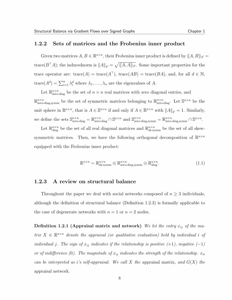
Definition 1.2.1 (Appraisal matrix and network) We let the entry xij of the ma-
trix X ∈ Rn×n denote the appraisal (or qualitative evaluation) held by individual i of
individual j. The sign of xij indicates if the relationship is positive (+1), negative (−1)
or of indifference (0). The magnitude of xij indicates the strength of the relationship. xii
can be interpreted as i’s self-appraisal. We call X the appraisal matrix, and G(X) the
appraisal network.
8

Structural Balance via Gradient Flows over Signed Graphs Chapter 1
Definition 1.2.2 (Heider’s axioms and social balance notions) The Heider’s ax-
ioms are
H1) A friend of a friend is a friend,
H2) An enemy of a friend is an enemy,
H3) A friend of an enemy is an enemy,
H4) An enemy of an enemy is a friend.
An appraisal network G(X) is structurally balanced in Heider’s sense, if it is complete
and satisfies axioms H1)-H4).
Consider a complete appraisal network G(X). We call a faction any group of agents
whose members positively appraise each other. We say two factions are antagonistic
if every representative from one faction negatively appraise every representative of the
other faction. It can be shown [76, 74, 38] that Heider’s structural balance condition for
G(X) with n ≥ 3 nodes holds if and only if either the individuals constitute a single
faction or can be partitioned into two antagonistic factions. The possession of the latter
property may thus be considered as an alternative definition of structural balance (and
is formally applicable to graphs without triads).
Definition 1.2.3 (Structural balance) A complete appraisal network G(X) is said
to satisfy structural balance, if G(X) is composed by one faction or two antagonistic
factions; or, whenever n ≥ 3, equivalently, that all triads are positive, i.e., xijxjkxki > 0
for any different i, j, k ∈ 1, . . . , n.
Notice that a structurally balanced graph is always sign-symmetric: sign(xij) =
sign(xji) for any i 6= j. For simplicity we will say that a matrix X corresponds to
structural balance whenever G(X) satisfies structural balance.
9

Structural Balance via Gradient Flows over Signed Graphs Chapter 1
1.3 Proposed models and representation as gradient
flows
In this section we propose our models defining them over the set of symmetric matri-
ces. We postponed the general asymmetric setting to Section 1.6.
1.3.1 Pure-influence model
We propose our new dynamic model solely based on interpersonal appraisals.
Definition 1.3.1 (Pure-influence model) The pure-influence model is a system of
differential equations on the set of zero-diagonal matrices Rn×nzero-diag defined by
xij =n∑
k=1k 6=i,j
xikxkj, (1.2)
for any i, j ∈ 1, . . . , n and i 6= j. Here xij, i 6= j, are the off-diagonal entries of a
zero-diagonal matrix X ∈ Rn×nzero-diag. In equivalent matrix form, the previous equations
read:
X = X2 − diag(X2), X(0) ∈ Rn×nzero-diag. (1.3)
We interpret X as the interpersonal appraisal matrix. While system (1.2) does not
define the evolution of self-appraisals, the matrix reformulation (1.3) ensures diag(X) =
0n×n and, since X(0) ∈ Rn×nzero-diag means diag(X(0)) = 0n×n, we have diag(X(t)) = 0n×n
for all positive times t.
Our model is a modification of the classical model proposed by Ku lakowski et al. [97],
where self-appraisals play a crucial role in the dynamics of the interpersonal appraisals.
10

Structural Balance via Gradient Flows over Signed Graphs Chapter 1
Definition 1.3.2 (Ku lakowski et al. model) The Ku lakowski et al. model is a sys-
tem of differential equations on the state space Rn×n defined by
xij =n∑
k=1
xikxkj = xij(xii + xjj) +n∑
k=1k 6=i,j
xikxkj, (1.4a)
xii = x2ii +
n∑
k=1k 6=i
xikxki, (1.4b)
for any i 6= j ∈ 1, . . . , n. In equivalent matrix form, the previous equations read:
X = X2.
Remark 1.3.1 (The problem with self-appraisals) The introduction of self-appraisals
in model (1.4) is objectionable on several grounds. The first conceptual problem is that
self-appraisals are not considered in any definition of structural balance in the social sci-
ences. Heider’s axioms in Definition 1.2.2 do not take into account self-appraisals: social
balance is a function of only interpersonal appraisals. Moreover, once self-appraisals are
introduced, one needs to postulate why and how self-appraisals affect interpersonal ap-
praisals, i.e., justify the choice of the first addendum for the right hand side of (1.4a).
Finally, one needs to postulate how they evolve, i.e., justify the choice for the right hand
side of (1.4b). In summary, the pure influence model (1.2) avoids these difficulties and
stays closer to the foundations of structural balance, in which individuals are attending
only to interpersonal appraisals. Even though X = X2 may appear mathematically sim-
pler or more elegant than X = X2 − diag(X2), we believe the latter model is actually
more parsimonious, lower dimensional, and more faithful to Heiders’ axioms.
One easily notices the following important property of the pure-influence model (1.3):
the right-hand side is an analytic function of X so that the equation enjoys (local)
existence and uniqueness of the solutions. A second property is that, if X(0) = X(0)>,
11

Structural Balance via Gradient Flows over Signed Graphs Chapter 1
then X(t) = X(t)> for all subsequent times. This implies that the pure-influence model
is well defined over the set of symmetric (zero diagonal) matrices Rn×nzero-diag,symm.
1.3.2 Dissonance function
We introduce and study the properties of a useful dissonance function that summarize
the total amount of cognitive dissonances [67] among the members of a social network due
to the lack of satisfaction of Heider’s axioms. Recall that, according to Definition 1.2.3,
a triad i→ j → k → i satisfies the axioms if and only if xijxjkxki > 0.
Definition 1.3.3 (Dissonance function) The dissonance function D : Rn×nzero-diag → R
is
D(X) = −n∑
i,j,k=1i 6=j,j 6=k,k 6=i
xijxjkxki = − trace(X3) = −n∑
i=1
λ3i , (1.5)
where λini=1 is the set of eigenvalues of X.
We plot D in a low-dimensional setting in Figure 1.1.
Energy landscapes in social balance theory are studied in [120, 63]. Our proposed dis-
sonance function is the extension to Rn×nzero-diag of the energy function proposed by [120] for
the setting of binary-valued symmetric appraisal matrices. For binary-valued appraisals,
the global minima of D correspond to networks that satisfy structural balance, since
all triads are positive (Definition 1.2.3). Thus, D naturally measures to which extent
Heider’s axioms are violated in a complete graph.
Lemma 1.3.2 (Properties of the dissonance function) Consider the dissonance func-
tion D and pick X ∈ Rn×nzero-diag. Then
(i) D is analytic and attains its maximum and minimum values on any compact matrix
subset of Rn×nzero-diag,
12

Structural Balance via Gradient Flows over Signed Graphs Chapter 1
Figure 1.1: For n = 3, an arbitrary symmetric unit-norm zero-diagonal matrixX ∈ Sn×nzero-diag,symm is described by (x12, x23, x31) with these coordinates living in the
sphere x212 + x2
23 + x231 = 1. In the upper figure, we plot this sphere with a heatmap,
with dark blue being the lowest value and light yellow the largest value, according tothe evaluation of the dissonance function D(X). The function has four global min-ima corresponding to the four possible configurations of G(X) satisfying structuralbalance, and we can qualitatively appreciate the convergence of solution trajectoriesto these minima in the superimposed vector field on the sphere. The lower figure is astereographic projection of the upper figure.
(ii) if G(X) satisfies structural balance, then D(X) < 0,
(iii) D(X) = D(X>),
(iv) D(X) = −〈〈X2, X>〉〉F .
Additionally, if ‖X‖F = 1, that is, X ∈ Sn×nzero-diag, then
(v) −1 ≤ D(X) ≤ 1.
Proof: Here we show only property (v), since the other properties follow easily from
13

Structural Balance via Gradient Flows over Signed Graphs Chapter 1
the definition of D. We note:
∥∥X2∥∥2
F=
n∑
i,j=1
(X2)2ij =
n∑
i,j=1
(Xi∗X∗j)2
≤n∑
i,j=1
‖Xi∗‖22‖X∗j‖2
2 =( n∑
i=1
‖Xi∗‖22
)( n∑
j=1
‖X∗j‖22
)
=(∑n
i,k=1x2ik
)2
= ‖X‖2F = 1.
Now, note that the Frobenius norm on the set of matrices coincides with the Euclidean
norm of a single vector obtained by stacking the column vectors of the matrix. Then,
by the Cauchy-Schwarz inequality applied to the inner-product 〈〈·, ·〉〉F , it follows that:
|D(X)| = |〈〈X2, X〉〉F | ≤ ‖X2‖F ‖X‖F ≤ (‖X‖F )3 ≤ 1 when ‖X‖F ≤ 1.
1.3.3 Transcription on the unit sphere and the projected pure-
influence model
We start by noting a simple fact. Given a trajectory X : R≥0 → Rn×nzero-diag \ 0n×n,
there exist unique trajectories η : R≥0 → R≥0 and Z : R≥0 → Sn×nzero-diag such that
X(t) = η(t)Z(t), where η(t) = ‖X(t)‖F and Z(t) = X(t)/ ‖X(t)‖F .
Theorem 1.3.3 (Transcription of the pure-influence model) The
pure-influence model (1.2) with initial conditions in Rn×nzero-diag,symm can be expressed as the
following system of differential equations:
Z = ηPZ⊥(Z2 − diag(Z2))
= η(Z2 − diag(Z2) +D(Z)Z), (1.6a)
η = −D(Z)η2, (1.6b)
14

Structural Balance via Gradient Flows over Signed Graphs Chapter 1
where η : R≥0 → R≥0 and Z : R≥0 → Sn×nzero-diag,symm. Here PZ⊥ is the orthogonal projection
onto spanZ⊥ in the vector space of square matrices with the Frobenius inner product.
Proof: Since X = ηZ+ηZ and X2−diag(X2) = η2 (Z2 − diag(Z2)), equation (1.3)
can be written as
ηZ + ηZ = η2(Z2 − diag(Z2)
). (1.7)
Differentiating the equality ‖Z(t)‖2F = 〈〈Z(t),Z(t)〉〉F = 1, one shows that 〈〈Z(t), Z(t)〉〉F =
0, that is, Z(t) ⊥ Z(t). Computing the Frobenius inner product with Z(t) on both sides
of (1.7), equation (1.6b) is immediate:
η = η2〈〈Z(t),Z2(t)− diag(Z2(t))〉〉F = η2〈〈Z(t),Z2(t)〉〉F = −D(Z(t))η2. (1.8)
where we have used the fact that Z(t) is symmetric, and that diag(Z(t)) = 0n×n and
hence 〈〈Z(t), diag(Z2(t))〉〉F = trace(Z(t)> diag(Z2(t))) = 0. Substituting (1.8) into
equation (1.7), one arrives at Z = η (Z2 − diag(Z2) +D(Z)).
Given Y ∈ Rn×n, let PZ(Y ) = 〈〈Y,Z〉〉FZ, i.e., PZ is the orthogonal projection
operator onto the linear space spanned by Z; and let PZ⊥(Y ) = Y − PZ(Y ) = Y −
〈〈Y,Z〉〉FZ be the orthogonal projection onto the space perpendicular to the linear space
spanned by Z. Then, we observe that PZ⊥(Z) = 0 and PZ⊥(Z) = Z. Using these
results, we apply PZ⊥ to both sides of (1.7) and obtain Z = ηPZ⊥(Z2− diag(Z2)). This
concludes the proof of equations (1.6).
In what follows, we are primarily interested in the dynamics (1.6a), describing the
behavior of the bounded component Z(t). From Lemma 1.8.1 we observe that η is a
time-scale change for (1.6a) and so, for our convenience, we get rid of it and obtain the
following dynamical system on the unit sphere.
Definition 1.3.4 (Projected pure-influence model) The projected pure-influence model
15

Structural Balance via Gradient Flows over Signed Graphs Chapter 1
is a system of differential equations on the manifold Sn×nzero-diag,symm defined by
Z = Z2 − diag(Z2) +D(Z)Z. (1.9)
Given a solution Z(t) to (1.9) with initial condition Z(0), Lemma 1.8.1 in the Appendix
shows that Z(t) is a time-scaled version of a solution Z(t) to (1.6a) with initial condition
Z(0) = Z(0), where η in (1.6b) can have any positive initial condition. Therefore, there
is a solution X(t) to (1.3) that is both a scaled and time-scaled version of Z(t).
Similarly, projecting onto the unit sphere leads to a new model based on the Ku lakowski
et al. model.
Definition 1.3.5 (Projected Ku lakowski et al. model) The projected Ku lakowski
et al. model is a system of differential equations on the manifold Sn×nzero-diag,symm defined by
Z(t) = Z2 +D(Z)Z. (1.10)
1.3.4 Pure-influence is the gradient flow of the dissonance func-
tion
We now let gradD denote the gradient vector field of the dissonance function D on
the manifold Rn×nzero-diag equipped with the Riemannian metric tensor 〈〈·, ·〉〉F . We also
let D∣∣Sn×nzero-diag,symm
denote the restriction of D onto the manifold Sn×nzero-diag,symm. We now
present the first of our main results.
Theorem 1.3.4 (The pure-influence models are gradient flows) Consider the pure-
influence model (1.2) with X(0) ∈ Rn×nzero-diag,symm and the projected pure-influence model (1.9)
with Z(0) ∈ Sn×nzero-diag,symm. Then
16
Structural Balance via Gradient Flows over Signed Graphs Chapter 1
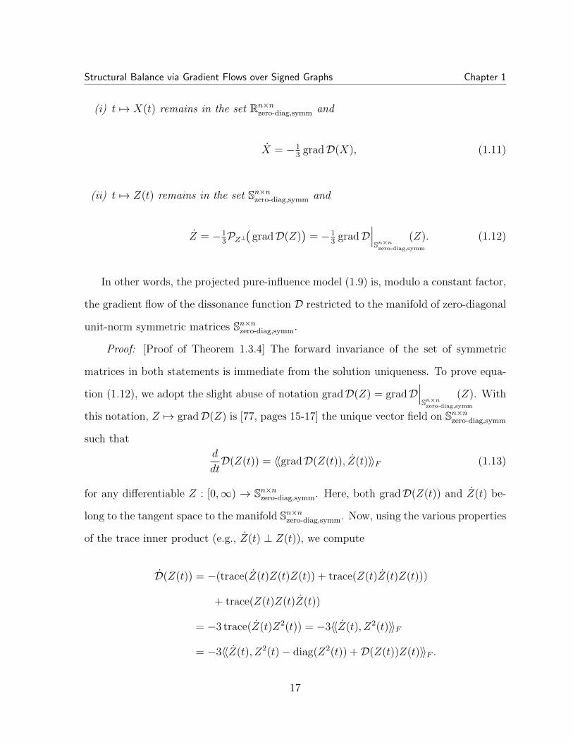
(i) t 7→ X(t) remains in the set Rn×nzero-diag,symm and
X = −13
gradD(X), (1.11)
(ii) t 7→ Z(t) remains in the set Sn×nzero-diag,symm and
Z = −13PZ⊥
(gradD(Z)
)= −1
3gradD
∣∣∣Sn×nzero-diag,symm
(Z). (1.12)
In other words, the projected pure-influence model (1.9) is, modulo a constant factor,
the gradient flow of the dissonance function D restricted to the manifold of zero-diagonal
unit-norm symmetric matrices Sn×nzero-diag,symm.
Proof: [Proof of Theorem 1.3.4] The forward invariance of the set of symmetric
matrices in both statements is immediate from the solution uniqueness. To prove equa-
tion (1.12), we adopt the slight abuse of notation gradD(Z) = gradD∣∣∣Sn×nzero-diag,symm
(Z). With
this notation, Z 7→ gradD(Z) is [77, pages 15-17] the unique vector field on Sn×nzero-diag,symm
such that
d
dtD(Z(t)) = 〈〈gradD(Z(t)), Z(t)〉〉F (1.13)
for any differentiable Z : [0,∞) → Sn×nzero-diag,symm. Here, both gradD(Z(t)) and Z(t) be-
long to the tangent space to the manifold Sn×nzero-diag,symm. Now, using the various properties
of the trace inner product (e.g., Z(t) ⊥ Z(t)), we compute
D(Z(t)) = −(trace(Z(t)Z(t)Z(t)) + trace(Z(t)Z(t)Z(t)))
+ trace(Z(t)Z(t)Z(t))
= −3 trace(Z(t)Z2(t)) = −3〈〈Z(t), Z2(t)〉〉F
= −3〈〈Z(t), Z2(t)− diag(Z2(t)) +D(Z(t))Z(t)〉〉F .
17

Structural Balance via Gradient Flows over Signed Graphs Chapter 1
Recalling that Z2 − diag(Z2) +D(Z)Z(1.6a)= PZ⊥(Z2 − diag(Z2)) belongs to the tangent
space to the manifold Sn×nzero-diag,symm at the point Z(t), one arrives at the equality
gradD(Z) = −3(Z2 − diag(Z2) +D(Z)Z
).
This concludes the proof of statement (ii). Finally, equation (1.11) can be proved in a
similar way.
1.4 Classification of symmetric equilibria
We here give the complete classification of the symmetric equilibria in the projected
pure-influence model (1.9); the classification of general asymmetric equilibria remains
an open problem. Thanks to Theorem 1.3.4, all symmetric equilibria of the projected
pure-influence model are critical points of the dissonance function D. We start with the
equilibrium equation:
Z2 +D(Z)Z − diag(Z2) = 0n×n, Z ∈ Sn×nzero-diag,symm. (1.14)
Note that the equilibria Z∗ with D(Z∗) = 0 correspond to equilibria of the original
system (1.3) X(t) ≡ X∗ = η(0)Z∗, whereas the others with D(Z∗) 6= 0 lead to
X(t) = η(t)Z∗, η(t) =η(0)
1 + tη(0)D(Z∗)
defined for t ∈ [0, 1η(0)D(Z∗)
) if D(Z∗) < 0 (for which the solution is unbounded) or for
t ≥ 0 if D(Z∗) > 0.
18

Structural Balance via Gradient Flows over Signed Graphs Chapter 1
1.4.1 Normalized Stiefel matrices
To start with, we introduce a special important manifold of non-square matrices that
we will use throughout the paper.
Definition 1.4.1 (Normalized Stiefel matrices) A matrix V ∈ Rn×k, for k ≤ n, is
normalized Stiefel (nSt), if
(i) the columns of V are pairwise orthogonal unit vectors, i.e., V >V = Ik;
(ii) the norm of each row is the same (obviously, it must be√k/n ≤ 1): diag(V V >) =
n−1kIn.
Let nSt(n, k) ⊆ Rn×k denote the set of normalized Stiefel matrices.
In general, the rows of an nSt matrix need not be orthogonal. We recall from [90] the
notion of compact Stiefel manifold, denoted by St(k, n) =X ∈ Rn×k | X>X = Ik
.
Lemma 1.4.1 (Characterization of nSt matrices) The set nSt(n, k), k ≤ n, is a
compact and analytic submanifold of Rn×k of dimension (k − 1)n + 1− k(k + 1)/2, and
it is also a submanifold of the compact Stiefel manifold (and thus, nSt(n, k) ⊆ St(k, n)).
Moreover,
(i) nSt(n, n) is the set of orthogonal matrices,
(ii) for k = 1, the matrix V is nSt if and only if
V =1√n
s1
...
sn
, (1.15)
for any numbers si ∈ −1,+1, i ∈ 1, . . . , n,19
Structural Balance via Gradient Flows over Signed Graphs Chapter 1
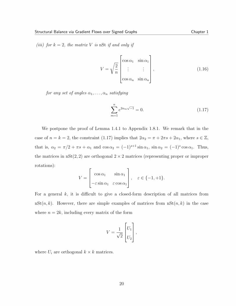
(iii) for k = 2, the matrix V is nSt if and only if
V =
√2
n
cosα1 sinα1
......
cosαn sinαn
, (1.16)
for any set of angles α1, . . . , αn satisfying
n∑
m=1
e2αm√−1 = 0. (1.17)
We postpone the proof of Lemma 1.4.1 to Appendix 1.8.1. We remark that in the
case of n = k = 2, the constraint (1.17) implies that 2α2 = π + 2πs+ 2α1, where s ∈ Z,
that is, α2 = π/2 + πs + α1 and cosα2 = (−1)s+1 sinα1, sinα2 = (−1)s cosα1. Thus,
the matrices in nSt(2, 2) are orthogonal 2× 2 matrices (representing proper or improper
rotations):
V =
cosα1 sinα1
−ε sinα1 ε cosα1
, ε ∈ −1,+1.
For a general k, it is difficult to give a closed-form description of all matrices from
nSt(n, k). However, there are simple examples of matrices from nSt(n, k) in the case
where n = 2k, including every matrix of the form
V =1√2
U1
U2
,
where Ui are orthogonal k × k matrices.
20

Structural Balance via Gradient Flows over Signed Graphs Chapter 1
1.4.2 Technical results
The classification of equilibria relies on the following technical results that will be
proved in Appendix 1.8.1.
Lemma 1.4.2 Suppose that Z2 − 2αZ = βIn for some symmetric n× n matrix Z with
diag(Z) = 0n×n and scalars α, β. Then Z can be decomposed as
Z = pV V > − qIn = Z> (1.18)
for some V ∈ nSt(n, k) (1 ≤ k < n) and constants p, q ≥ 0 such that pk = qn, 2α = p−2q
and β = q(p− q). Namely, p = 2√α2 + β, q =
√α2 + β − α.
Corollary 1.4.3 Given a matrix Z = Z> with diag(Z) = 0n×n, the matrix Z2 − 2αZ is
diagonal with s different eigenvalues β1 < . . . < βs of multiplicities n1, . . . , ns respectively
(n1 + n2 + . . .+ ns = n) if and only if there exists such a permutation matrix S that
SZS−1 = diag(Z1, . . . , Zs),
where each Zi is decomposed as (1.18) with parameters pi, qi, Vi, where Vi ∈ nSt(ni, ki)
for some ki < ni and
pi = 2√α2 + βi, qi =
√α2 + βi − α. (1.19)
Thus, for irreducible Z = Z> the matrix Z2 − 2αZ is diagonal if and only if Z is
decomposed as (1.18) with p, q ≥ 0.
21

Structural Balance via Gradient Flows over Signed Graphs Chapter 1
1.4.3 Classification of irreducible symmetric equilibria
Theorem 1.4.4 (Irreducible equilibria for the projected pure-influence model)
For the projected pure-influence model (1.9),
(i) all irreducible symmetric equilibria are of the form
Z∗ = pV V > − qIn, (1.20)
with V ∈ nSt(n, k), 1 ≤ k < n, and
p =
√n
k(n− k), q =
√k
n(n− k); (1.21)
(ii) Z∗ has k positive eigenvalues with value p− q and n− k negative eigenvalues with
value −q;
(iii) the dissonance function satisfies
D(Z∗) = − n− 2k√kn(n− k)
, (1.22)
and the right-hand side is monotonically increasing in k ∈ 1, . . . , n − 1 (see
Figure 1.2).
Proof: We start by proving a technical statement. Pick V ∈ nSt(n, k), p, q real
numbers and set θ = p − 2q. Then, the matrix Z = pV V > − qIn = Z> satisfies the
following properties:
(a) Z2 − θZ = q(p− q)In, and thus diag(Z2) = θ diag(Z) + q(p− q)In;
(b) for any p 6= 0, the matrix Z has two eigenvalues p−q and (−q) whose multiplicities
are k and (n− k) respectively;
22

Structural Balance via Gradient Flows over Signed Graphs Chapter 1
k<latexit sha1_base64="kBpW2Z3PaYvSRudv/tWr0IjE0ec=">AAAB6HicbVBNS8NAEJ3Ur1q/qh69LBbBU0mqoHgqePHYgq2FNpTNdtKu3WzC7kYoob/AiwdFvPqTvPlv3LY5aOuDgcd7M8zMCxLBtXHdb6ewtr6xuVXcLu3s7u0flA+P2jpOFcMWi0WsOgHVKLjEluFGYCdRSKNA4EMwvp35D0+oNI/lvZkk6Ed0KHnIGTVWao775Ypbdecgq8TLSQVyNPrlr94gZmmE0jBBte56bmL8jCrDmcBpqZdqTCgb0yF2LZU0Qu1n80On5MwqAxLGypY0ZK7+nshopPUkCmxnRM1IL3sz8T+vm5rw2s+4TFKDki0WhakgJiazr8mAK2RGTCyhTHF7K2EjqigzNpuSDcFbfnmVtGtV76Jaa15W6jd5HEU4gVM4Bw+uoA530IAWMEB4hld4cx6dF+fd+Vi0Fpx85hj+wPn8AdFrjOs=</latexit>
D(Z(k))<latexit sha1_base64="ovGXA4hPUH04K0r9pfS9FoReDeY=">AAACBnicbZDLSsNAFIYnXmu9Rbt0M1iEVqQkVVBcFXThsoK9YBvLZDpth04mYWZSDKF738KtbtyJW19D8GGcpFlo64GBj/8/hznndwNGpbKsL2NpeWV1bT23kd/c2t7ZNff2m9IPBSYN7DNftF0kCaOcNBRVjLQDQZDnMtJyx1eJ35oQIanP71QUEMdDQ04HFCOlpZ5Z6HpIjTBi8fW0dP9wXBqXyz2zaFWstOAi2BkUQVb1nvnd7fs49AhXmCEpO7YVKCdGQlHMyDTfDSUJEB6jIelo5Mgj8kROhik48WN6xhQeaa8PB77QjyuYqr9nY+RJGXmu7kyWlvNeIv7ndUI1uHBiyoNQEY5nHw1CBpUPk0xgnwqCFYs0ICyo3hriERIIK51cXsdhzx+/CM1qxT6tVG/PirXLLJgcOACHoARscA5q4AbUQQNgEIFn8AJejSfjzXg3PmatS0Y2UwB/yvj8AYqhmAo=</latexit>
1<latexit sha1_base64="SuH2nvDxfbvCsFOsx6u5Rfuy1ew=">AAAB8nicbZBNS8NAEIY3ftb6VfXoJVgED1KSWtBjwYvHFuwHtKFstpN26WYTdifFEvoLvOrFm3j1Dwn+GLdpDtr6wsLDvDPszOvHgmt0nC9rY3Nre2e3sFfcPzg8Oi6dnLZ1lCgGLRaJSHV9qkFwCS3kKKAbK6ChL6DjT+4XfmcKSvNIPuIsBi+kI8kDziiaUtMdlMpOxclkr4ObQ5nkagxK3/1hxJIQJDJBte65ToxeShVyJmBe7CcaYsomdAQ9g5KGoK/1dJSBlz5lK8/tS+MN7SBS5km0s+rv2ZSGWs9C33SGFMd61VsU//N6CQZ3XsplnCBItvwoSISNkb243x5yBQzFzABliputbTamijI0KRVNHO7q8evQrlbcm0q1WSvXa3kwBXJOLsgVccktqZMH0iAtwgiQZ/JCXi203qx362PZumHlM2fkj6zPH5VgkO8=</latexit>
2<latexit sha1_base64="B8F9aP8S15+xIQddnwvRo6/LBGg=">AAAB8nicbZDLSgNBEEVrfMb4irp00xgEFxJmYkCXATcuEzAPSIbQ0+lJmvQ86K4JhiFf4FY37sStPyT4MXYms9DECw2HulV01fViKTTa9pe1sbm1vbNb2CvuHxweHZdOTts6ShTjLRbJSHU9qrkUIW+hQMm7seI08CTveJP7hd+ZcqVFFD7iLOZuQEeh8AWjaErN6qBUtit2JrIOTg5lyNUYlL77w4glAQ+RSap1z7FjdFOqUDDJ58V+onlM2YSOeM9gSAOur/V0lIGbPmUrz8ml8YbEj5R5IZKs+ns2pYHWs8AznQHFsV71FsX/vF6C/p2bijBOkIds+ZGfSIIRWdxPhkJxhnJmgDIlzNaEjamiDE1KRROHs3r8OrSrFeemUm3WyvVaHkwBzuECrsCBW6jDAzSgBQw4PMMLvFpovVnv1seydcPKZ87gj6zPH5bukPA=</latexit>
3<latexit sha1_base64="QWzxZfxRqjEzfC+a8H1iE2gRG+E=">AAAB8nicbZBNS8NAEIYn9avWr6pHL8EieJCStAU9Frx4bMF+QBvKZjtpl242YXdTLKW/wKtevIlX/5Dgj3Gb5qCtLyw8zDvDzrx+zJnSjvNl5ba2d3b38vuFg8Oj45Pi6VlbRYmk2KIRj2TXJwo5E9jSTHPsxhJJ6HPs+JP7pd+ZolQsEo96FqMXkpFgAaNEm1KzOiiWnLKTyt4EN4MSZGoMit/9YUSTEIWmnCjVc51Ye3MiNaMcF4V+ojAmdEJG2DMoSIjqRk1HKXjzp3TlhX1lvKEdRNI8oe20+nt2TkKlZqFvOkOix2rdWxb/83qJDu68ORNxolHQ1UdBwm0d2cv77SGTSDWfGSBUMrO1TcdEEqpNSgUTh7t+/Ca0K2W3Wq40a6V6LQsmDxdwCdfgwi3U4QEa0AIKCM/wAq+Wtt6sd+tj1Zqzsplz+CPr8weYfJDx</latexit>
6<latexit sha1_base64="/gZr+S3+jbjEpburPSS3pcnTZpE=">AAAB8nicbZDLSgNBEEV74ivGV9Slm8YguJAwE4O6DLhxmYB5QDKEnk5N0qTnQXdNMIR8gVvduBO3/pDgx9iZzEITLzQc6lbRVdeLpdBo219WbmNza3snv1vY2z84PCoen7R0lCgOTR7JSHU8pkGKEJooUEInVsACT0LbG98v/PYElBZR+IjTGNyADUPhC87QlBo3/WLJLtup6Do4GZRIpnq/+N0bRDwJIEQumdZdx47RnTGFgkuYF3qJhpjxMRtC12DIAtBXejJMwZ09pSvP6YXxBtSPlHkh0rT6e3bGAq2ngWc6A4Yjveotiv953QT9O3cmwjhBCPnyIz+RFCO6uJ8OhAKOcmqAcSXM1pSPmGIcTUoFE4ezevw6tCpl57pcaVRLtWoWTJ6ckXNySRxyS2rkgdRJk3AC5Jm8kFcLrTfr3fpYtuasbOaU/JH1+QOdJpD0</latexit>
7<latexit sha1_base64="dgqnO3JkXCTlMmT8lEvNp+xoQxc=">AAAB8nicbZBNS8NAEIY39avWr6pHL8EieJCS1EI9Frx4bMF+QBvKZjtpl242YXdSLKW/wKtevIlX/5Dgj3Gb5qCtLyw8zDvDzrx+LLhGx/myclvbO7t7+f3CweHR8Unx9Kyto0QxaLFIRKrrUw2CS2ghRwHdWAENfQEdf3K/9DtTUJpH8hFnMXghHUkecEbRlJq1QbHklJ1U9ia4GZRIpsag+N0fRiwJQSITVOue68TozalCzgQsCv1EQ0zZhI6gZ1DSEPSNno5S8OZP6coL+8p4QzuIlHkS7bT6e3ZOQ61noW86Q4pjve4ti/95vQSDO2/OZZwgSLb6KEiEjZG9vN8ecgUMxcwAZYqbrW02pooyNCkVTBzu+vGb0K6U3dtypVkt1atZMHlyQS7JNXFJjdTJA2mQFmEEyDN5Ia8WWm/Wu/Wxas1Z2cw5+SPr8weetJD1</latexit>
8<latexit sha1_base64="kXT81pEbbeHr1AAqduWlFBDkKpc=">AAAB8nicbZBNS8NAEIY39avWr6pHL8EieJCS1II9Frx4bMF+QBvKZjtpl242YXdSLKW/wKtevIlX/5Dgj3Gb5qCtLyw8zDvDzrx+LLhGx/myclvbO7t7+f3CweHR8Unx9Kyto0QxaLFIRKrrUw2CS2ghRwHdWAENfQEdf3K/9DtTUJpH8hFnMXghHUkecEbRlJq1QbHklJ1U9ia4GZRIpsag+N0fRiwJQSITVOue68TozalCzgQsCv1EQ0zZhI6gZ1DSEPSNno5S8OZP6coL+8p4QzuIlHkS7bT6e3ZOQ61noW86Q4pjve4ti/95vQSDmjfnMk4QJFt9FCTCxshe3m8PuQKGYmaAMsXN1jYbU0UZmpQKJg53/fhNaFfK7m250qyW6tUsmDy5IJfkmrjkjtTJA2mQFmEEyDN5Ia8WWm/Wu/Wxas1Z2cw5+SPr8wegQpD2</latexit> 9
<latexit sha1_base64="xizxjHLqXodHhPVcPYXRVetjnYs=">AAAB8nicbZDLSgNBEEV74ivGV9Slm8YguJAwEwPqLuDGZQLmAckQejo1SZOeB901wRDyBW51407c+kOCH2NnMgtNvNBwqFtFV10vlkKjbX9ZuY3Nre2d/G5hb//g8Kh4fNLSUaI4NHkkI9XxmAYpQmiiQAmdWAELPAltb3y/8NsTUFpE4SNOY3ADNgyFLzhDU2rc9Yslu2ynouvgZFAimer94ndvEPEkgBC5ZFp3HTtGd8YUCi5hXuglGmLGx2wIXYMhC0Bf6ckwBXf2lK48pxfGG1A/UuaFSNPq79kZC7SeBp7pDBiO9Kq3KP7ndRP0b92ZCOMEIeTLj/xEUozo4n46EAo4yqkBxpUwW1M+YopxNCkVTBzO6vHr0KqUnetypVEt1apZMHlyRs7JJXHIDamRB1InTcIJkGfyQl4ttN6sd+tj2ZqzsplT8kfW5w+h0JD3</latexit>
0.0<latexit sha1_base64="iLVoW7F6VuuianoiFhaam0OCR3o=">AAAB9HicbZDLSsNAFIZP6q3WW9Wlm8EiuJCSVEGXBTcuK9oLtKFMppN06GQSZibFEvoIbnXjTtz6PoIP4yTNQlsPzPDx/+cwZ34v5kxp2/6ySmvrG5tb5e3Kzu7e/kH18KijokQS2iYRj2TPw4pyJmhbM81pL5YUhx6nXW9ym/ndKZWKReJRz2LqhjgQzGcEayM92HV7WK2ZOy+0Ck4BNSiqNax+D0YRSUIqNOFYqb5jx9pNsdSMcDqvDBJFY0wmOKB9gwKHVF2oaZCDmz7lS8/RmfFGyI+kOUKjXP09m+JQqVnomc4Q67Fa9jLxP6+faP/GTZmIE00FWTzkJxzpCGUJoBGTlGg+M4CJZGZrRMZYYqJNThUTh7P8+VXoNOrOZb1xf1Vr2kUwZTiBUzgHB66hCXfQgjYQCOAZXuDVmlpv1rv1sWgtWcXMMfwp6/MHbz2RXA==</latexit>
0.5<latexit sha1_base64="hx7kpbKdb3plQ/fXa6RTJ0mtOSs=">AAAB9HicbZDLSsNAFIZPvNZ6q7p0M1gEFxKSquiy4MZlRXuBNpTJdJIOnUzCzKRYQh/BrW7ciVvfR/BhnKZZaOuBgY//P4dz5vcTzpR2nC9rZXVtfWOztFXe3tnd268cHLZUnEpCmyTmsez4WFHOBG1qpjntJJLiyOe07Y9uZ357TKVisXjUk4R6EQ4FCxjB2kgPjn3Vr1Qd28kLLYNbQBWKavQr371BTNKICk04VqrrOon2Miw1I5xOy71U0QSTEQ5p16DAEVXnahzm4GVP+dFTdGq8AQpiaZ7QKFd/z2Y4UmoS+aYzwnqoFr2Z+J/XTXVw42VMJKmmgswXBSlHOkazBNCASUo0nxjARDJzNSJDLDHRJqeyicNd/PwytGq2e2HX7i+rdacIpgTHcAJn4MI11OEOGtAEAiE8wwu8WmPrzXq3PuatK1YxcwR/yvr8AXcDkWE=</latexit>
0.5<latexit sha1_base64="SThrAYV/ZxOG9tGCHEKUlnXTRhc=">AAAB9XicbZDLSsNAFIZP6q3WW9Wlm8EiuNCQVEWXBTcuK9gLtKFMppN26GQSZibVEvoKbnXjTtz6PIIP46TNQlsPDHz8/zmcM78fc6a043xZhZXVtfWN4mZpa3tnd6+8f9BUUSIJbZCIR7LtY0U5E7Shmea0HUuKQ5/Tlj+6zfzWmErFIvGgJzH1QjwQLGAE60w6d+yrXrni2M6s0DK4OVQgr3qv/N3tRyQJqdCEY6U6rhNrL8VSM8LptNRNFI0xGeEB7RgUOKTqTI0HM/DSp9nVU3RivD4KImme0Gim/p5NcajUJPRNZ4j1UC16mfif10l0cOOlTMSJpoLMFwUJRzpCWQSozyQlmk8MYCKZuRqRIZaYaBNUycThLn5+GZpV272wq/eXlZqTB1OEIziGU3DhGmpwB3VoAIEhPMMLvFqP1pv1bn3MWwtWPnMIf8r6/AHicpGY</latexit>
Figure 1.2: For a network with size n = 10, the dissonance function D evaluated onall irreducible symmetric equilibria with k ∈ 1, . . . , 9 positive eigenvalues, accordingto equation (1.22).
(c) the eigenspaces corresponding to p − q and −q are the image of V and the kernel
of V > respectively;
(d) diag(Z) = 0n×n if and only if pk = qn; in this situation, trace(Z2) = q(p− q)n and
D(Z) = − trace(Z2Z>) = −θnq(p− q).
To prove (a), recall that V >V = Ik and therefore
Z2 = p2V V >V V > + q2In − 2pqV V > = pθV V > + q2In = θZ + (pq − q2)In.
To prove (b) and (c), notice that for any vector z = V y one has V V >z = V (V >V )y =
V y = z, and thus Zz = (p − q)z. The space of such vectors is nothing else than the
image of V and has dimension k (recall that the columns of V are orthogonal, and hence
are linearly independent). If V >z = 0, then Zz = −qz, and the dimension of ker(V >) is
(n− k). Since Z = Z> and p− q 6= −q (except for the case where p = q = 0 and Z = 0,
which is trivial), the two eigenspaces are orthogonal and their sum coincides with Rn.
Hence, there are no other eigenvalues. To prove (d), note first p diag(V V >) = (pk/n)In,
and thus diag(Z) = 0n×n if and only if pk/n = q. Using statement (a), one shows that
in this situation diag(Z2) = q(p− q)In and hence trace(Z2) = q(p− q)n. Thanks to (a),
23

Structural Balance via Gradient Flows over Signed Graphs Chapter 1
Z3 = θZ2 + q(p− q)Z =⇒ trace(Z3) = θ trace(Z2) = θnq(p− q), which finishes the proof
of (d).
Now, to prove the statement (i) of the theorem, let Z∗ be an irreducible symmetric
solution to equation (1.14). For α = −D(Z∗)/2, the matrix (Z∗)2 − 2αZ∗ = diag(Z∗2)
is diagonal. Since Z∗ is irreducible, it follows from Corollary 1.4.3 that Z∗ can be de-
composed as (1.20) with some p, q ≥ 0. Then, from (a) and (d), it also follows that Z∗
satisfies equation (1.14) if and only if pk = qn (which comes from diag(Z∗) = 0n×n) and
pq − q2 = 1/n (which comes from trace(Z∗2) = 1). This implies that q =√
kn(n−k)
and
p =√
nk(n−k)
.
Finally, statement (ii) follows from (b); and (iii) is obtained by substituting the values
of p and q into the definition of the dissonance function (1.5) and noting that the smooth
function κ 7→ − n−2κ√nκ(n−κ)
has positive derivative on (0, n).
1.4.4 Classification of reducible symmetric equilibria
The next theorem generalizes Theorem 1.4.4 and characterizes all symmetric equilib-
ria for the projected pure-influence model and its proof can be found in Appendix 1.8.1.
Theorem 1.4.5 (All equilibria for the projected pure-influence model) The ma-
trix Z∗ is an equilibrium (1.14) of the projected pure-influence model if and only if a
permutation matrix S exists such that:
(i) SZ∗S−1 = diag(Z∗1 , . . . , Z∗s ), s ≥ 1, Z∗i = Z∗i
> ∈ Rni×ni;
(ii) the blocks Z∗i admit representation (1.18): Z∗i = piViV>i − qiIni, where pi, qi ≥ 0
and Vi ∈ nSt(ni, ki), 1 ≤ ki < ni;
(iii) the sign ε = sign(ni − 2ki) ∈ −1, 0, 1 is the same for all i = 1, . . . , s such that
Z∗i 6= 0ni×ni and
24

Structural Balance via Gradient Flows over Signed Graphs Chapter 1
(iv) each block Z∗i 6= 0ni×ni is irreducible and the corresponding coefficients pi, qi have
the form
pi = 2√α2 + βi, qi =
√α2 + βi − α, (1.23)
where
(a) for ε 6= 0, α and βi are determined from
α = ε
( ∑
i:Zi 6=0
4kini(ni − ki)(ni − 2ki)2
)−1/2
,
βi = α2 4niki − 4k2i
(ni − 2ki)2;
(1.24)
(b) for ε = 0, α = 0, for all i, and βi are chosen in such a way that∑
i:Zi 6=0 βini =
1.
Remark 1.4.6 Let Z∗ be a reducible equilibrium for the projected pure-influence model
such that G(Z∗) is composed of m (disconnected) subgraphs that satisfy structural bal-
ance. According to Definition 1.2.3, G(Z∗) does not satisfy structural balance since this
definition requires G(Z∗) to be complete.
1.4.5 Structural balance and equilibria
We now characterize the equilibria corresponding to structural balance and how they
minimize the dissonance function.
Corollary 1.4.7 (Balanced equilibria of the projected pure-influence model) For
the projected pure-influence model (1.9), let Z∗ ∈ Sn×nzero-diag be an equilibrium point with a
single positive eigenvalue. Then,
25

Structural Balance via Gradient Flows over Signed Graphs Chapter 1
(i) after a relabelling of the agents, Z∗ has the form
Z∗ =
Z ′ 0n1×(n−n1)
0(n−n1)×n1 0(n−n1)×(n−n1)
(1.25)
with n1 ≤ n and
Z ′ =1√
n1(n1 − 1)(ss> − In1), (1.26)
for some s ∈ −1,+1n1; and thus, for any fixed n1, there are only 2n1−1 different
equilibria (with a single positive eigenvalue),
(ii) G(Z ′) satisfies structural balance, with the binary vector s characterizing the dis-
tribution of the individuals in the single faction or in the two factions, and
(iii) if G(Z∗) is a connected graph, then G(Z∗) satisfies structural balance (being thus
complete) and Z∗ is a global minimizer to the optimization problem:
minimizeZ∈Rn×n
D(Z)
subject to Z ∈ Sn×nzero-diag,symm
and satisfies D(Z∗) = − n−2√n(n−1)
.
Proof:
Consider a permutation of indices from Theorem 1.4.5. Since Z∗ has only one positive
eigenvalue, it can have only one non-zero diagonal block Z∗i = Z ′. Statement (i) now
follows from (1.20),(1.21) (with k = 1, n = n1) and (1.15).
Regarding statement (ii), observe that for any different i, j and k,
z′ijz′jkz′ki =
(sisj)(sjsk)(sksi)
(n1(n1 − 1))3/2=
1
(n1(n1 − 1))3/2> 0.
26

Structural Balance via Gradient Flows over Signed Graphs Chapter 1
This inequality implies sign(z′ij) = sign(z′jkz′ki) and thus we know that Z ′ satisfies struc-
tural balance. It is immediate to see that any i and j such that si = sj correspond to
the same faction in the network G(Z ′). This completes the proof for (ii).
Regarding statement (iii), we notice that the smooth function η 7→ − η−2√η(η−1)
has
negative derivative for η > 3/2. Hence, the value of D(Z∗) = D(Z ′) = − n1−2√n1(n1−1)
at
equilibrium (1.25) with one positive eigenvalue is minimal when Z ′ = Z∗ and n1 = n,
that is, the matrix is irreducible. Now, let us focus on the points that vanish the gradient
of D, i.e., the equilibria of the projected pure-influence model. Permuting the agents,
we may confine ourselves to equilibria described in Theorem 1.4.5 that have s blocks
of size ni with ki < ni positive eigenvalues, i ∈ 1, . . . , s. To see why this is true,
in the proof of Theorem 1.4.4 it was shown that D(Z∗i ) = −2αnqi(pi − qi) = −2αβi.
Next, if ε = −1, then α < 0 and D(Z∗) > 0. If ε = sign(ni − 2ki) = 0 for all
Z∗i 6= 0, then D(Z∗) =∑
iD(Z∗i ) = 0. As we know, the minimal value should be
negative, so such equilibria cannot be global minimizers. Therefore, we may assume
that ε = 1, that is, ki < ni/2 for all such i that Z∗i 6= 0. Assume, without loss of
generality, that Z∗1 , . . . , Z∗m 6= 0 and Z∗m+1, . . . , Z
∗s = 0. Denote k1 + · · · + km = k′ and
n1 + · · · + nm = n′ ≤ n. Note that the function f(ξ) = ξ(1 − ξ)/(1 − 2ξ)2 is convex on
(0, 1/2). Therefore, Jensen’s inequality implies
1
n
m∑
i=1
kini(ni − ki)(ni − 2ki)2
=m∑
i=1
ninf(kini
)≥ f
( m∑
i=1
kin′
)= f
(k′n′
)=
k′(n′ − k′)(n′ − 2k′)2
,
and, in turn,
D(Z∗) = −(
m∑
i=1
kini(ni − ki)(ni − 2ki)2
)−1/2
≥ − n′ − 2k′√k′n′(n′ − k′)
.
We know, however from Theorem 1.4.4 that the right-hand side is minimal when k′ = 1,
27

Structural Balance via Gradient Flows over Signed Graphs Chapter 1
in which case the minimal value, as we have seen in the beginning in the proof, is achieved
at n′ = n. Hence, the irreducible equilibrium with one positive eigenvalue is the global
minimizer of D∗.
Remark 1.4.8 Let Z∗ denote an equilibrium point with one positive eigenvalue. Then,
−Z∗ has one negative eigenvalue and does not correspond to structural balance. All such
−Z∗ correspond to isolated critical points of D.
1.4.6 Examples of equilibria with two positive eigenvalues
Let Z∗ be any equilibrium of the projected pure-influence model parameterized by
nSt(n, 2) matrices, so that it has two positive eigenvalues. Let us assume first that it is
irreducible. Then, another class of equilibria is found using the parametrization (1.16).
It can be easily shown that
Z∗ =
√2
n(n− 2)(θij)
ni,j=1, θij =
0, i = j
cos(αi − αj), i 6= j.
Here the angles αi should satisfy the relation (1.17). Interestingly, many of such matrices
do not correspond to structural balance. Consider, for example, the case where the unit
vectors in (1.17) constitute a regular n-gon: αi = π(i−1)n
, i = 1, . . . , n. For any pair i, j > i
the entry zij is negative if (j − i) > n/2, positive if j − i < n/2 and zero if j − i = n/2
(possible only for even n). If n is odd, the graph is complete, otherwise, the pairs of
nodes (i, i + n/2) for i = 1, . . . , n/2 are not connected. For example, in the smallest
28

Structural Balance via Gradient Flows over Signed Graphs Chapter 1
dimension n = 3, by setting α1 = 0, α2 = π/3 and 2π/3, we obtain the equilibrium
Z∗ =1√6
0 +1 −1
+1 0 +1
−1 +1 0
which does not correspond to structural balance. Actually, in the case where n = 3 or
n ≥ 5, the graph always contains imbalanced triads. For instance, for n ≥ 3 being odd
the nodes i = 1, j = (n− 1)/2 and ` = (n+ 3)/2 always constitute such a triad: zi` < 0,
whereas zij, zj` ≥ 0. For an even number n ≥ 6, one may take i = 1, j = n/2, ` = n/2+2.
In the case n = 4, the equilibrium Z∗ corresponds to an incomplete cyclic graph such
that D(Z∗) = 0:
Z∗ =1
2√
2
0 1√2
0 − 1√2
1√2
0 1√2
0
0 1√2
0 1√2
− 1√2
0 1√2
0
.
For the reducible matrix case, since Z∗ has two positive eigenvalues, G(Z∗) contains
two disconnected subgraphs that satisfy structural balance with possibly other isolated
nodes.
1.5 Convergence to balanced equilibria and stability
analysis
We now provide convergence results for our models towards equilibria that correspond
to structural balance. We present a supporting lemma and then our main theorem.
Lemma 1.5.1 Assume that the solution of (1.2) satisfies xi∗(t0) = 01×n at some t0 ≥ 0,
29

Structural Balance via Gradient Flows over Signed Graphs Chapter 1
that is, in the graph G(X(t0)) node i does not communicate to any other node. Then,
xi∗(t) ≡ 01×n for any t ≥ 0. The same holds for the solutions of (1.9).
Proof: Since the right-hand sides of (1.2) and (1.9) are analytic, any solution is a
real-analytic function of time. Assuming that xij(t0) = 0 for all j, one finds that xij(t0) =
0. Differentiating (1.2), it is easy to show that xij(t0) = 0, and so on, x(m)ij (t0) = 0 for
any m ≥ 1. In view of analyticity, one has xij(t) ≡ 0 for any t. Similarly, zij(t0) = 0∀j
entails that zij(t) ≡ 0 for any solution of (1.9).
Theorem 1.5.2 (Convergence results and dynamical properties) Consider the pure-
influence model (1.2) with an initial condition X(0) ∈ Rn×nzero-diag,symm and the projected
pure-influence model (1.9) with initial condition Z(0) = X(0)‖X(0)‖F
. Then,
(i) the solution Z(t) converges to a single critical point of the dissonance function D;
(ii) the number of negative eigenvalues of Z(t) is non-decreasing.
Moreover, if X(0) has one positive eigenvalue, then
(iii) limt→+∞ Z(t) = Z∗, where Z∗ is as in (1.26), so that G(Z(t)) or one of its connected
components (while the rest of nodes are isolated) reaches structural balance in finite
time;
(iv) X(t) achieves the same sign structure as Z∗ in finite time;
(v) nonzero entries of X(t) diverge to infinity in finite time.
Proof: For convenience, throughout this proof, let us denote W (t) = X(t)‖X(t)‖F
, i.e.,
X(t) = η(t)W (t) with η(t) evolving according to (1.6a) and W (t) evolving according
to (1.6b). From the construction of the transcription of the pure-influence model in
Theorem 1.3.3, we have that η(t) = ‖X(t)‖F and so η(t) > 0 for all well-defined t ≥ 0.
30

Structural Balance via Gradient Flows over Signed Graphs Chapter 1
Moreover, Lemma 1.8.1 let us conclude that W (t) = Z(∫ t
0η(s)ds) for all t ≥ 0, and thus
the solution X(t) is well defined.
To prove (i), recall that (1.9) is a gradient flow dynamics of the analytic function D,
and the trajectory Z(t) stays on a compact manifold and, in particular, is bounded. The
classical result of Lojasiewicz [3] implies convergence of the trajectory to a single fixed
point.
To prove (ii), we enumerate the eigenvalues of Z(t) in the descending order λ1(t) ≥
λ2(t) . . . ≥ λn(t) and consider the corresponding orthonormal bases of eigenvectors vi(t).
Since Zi(t)vi(t) = λi(t)vi(t) and vi(t)>vi(t) = 1, we obtain Zvi + Zvi = λivi + λivi and
vi(t)>vi(t) = 0. Therefore,
λi = v>i Zvi + v>i Zvi = v>i Zvi + λiv>i vi = v>i Zvi,
entailing the following differential equation
λi = λ2i +D(Z)λi − v>i diag(Z2)vi. (1.27)
Notice that all diagonal entries of diag(Z2) are nonnegative. Now, due to Lemma 1.5.1,
if the ith row of X was initially the zero vector, then it will continue being the same for
all times and also for Z; and, moreover, diag(Z2)ii = 0 and there exists a zero eigenvalue
with its associated eigenvector having zero entries in all the positions of the entries where
diag(Z2) are positive. Then, it immediately follows from (1.27) that if λi(0) = 0 due to
Z(0) having a row being the zero vector 01×n, then λi = 0.
Now, let N be the set of indices i such that diag(Z2)ii > 0. Thus, for any i ∈ N , if
31

Structural Balance via Gradient Flows over Signed Graphs Chapter 1
λi crosses the real axis at time t∗, i.e., λ(t∗) = 0, then
λi(t∗) = −(vi(t
∗))> diag (Z2(t∗))vi(t∗) < 0. (1.28)
Therefore, if λi(t0) ≤ 0 for some t0 ≥ 0, then λi(t) ≤ 0 for all t ≥ t0. This finishes the
proof for (ii).
Notice that since trace(Z(t)) = 0 and Z(t) = Z(t)> 6= 0n×n, then Z(t) has at least
one positive eigenvalue. Then, equation (1.28) implies that
Λ :=Z ∈ Sn×nzero-diag,symm | Z has only one positive eigenvalue
is forward invariant and, in particular, the limit Z∗ = limt→∞ Z(t) (existing in view of
statement (i)) belongs to Λ. Since Z∗ is a critical point of D (or, in view of Theorem 1.3.4,
the equilibrium of (1.9)), it has the structure described by Corollary 1.4.7.
By continuity of the flow Z(t), there is a finite time τ such that G(Z(t)) has the same
sign structure as G(Z∗) for all t ≥ τ . This finishes the proof for (iii).
Now we prove the last two statements of the theorem. Knowing the convergence
result from (iii), Lemma 1.8.1 tells us that introducing the term η as in the transcribed
system (1.6a) to the projected pure-influence model has the simple effect of altering
the convergence rate properties for Z(t). Therefore, there always exist a finite time
τ ∗ ≥ 0 such that, for any t ≥ τ ∗, W (t) satisfies the sign properties of statement (iii)
regarding structural balance. Moreover, the fact that X(t) = η(t)W (t) and η(t) ≥ 0
by construction, immediately implies (iv). Now, let g(t) := −D(W (t)), and notice that
g(t) is a strictly positive continuous function for all (well-defined) t ≥ τ ∗. Now, from
equation (1.6b), we have the system η(t) = g(t)η2(t), with solution η(t) = η(τ)
1−η(τ)∫ tτ g(s)ds
for t ≥ τ . Then, since∫ tτg(s)ds is a monotonic strictly increasing function on t ≥ τ ,
32
Structural Balance via Gradient Flows over Signed Graphs Chapter 1
we have that η(t) → +∞ as t → t∗, where t∗ > τ ∗ is some finite time such that∫ t∗τg(s)ds = 1
η(τ)(note that t∗ > τ ∗ holds from the relationship W (t) = Z(
∫ t0η(s)ds)).
Then, we conclude that the solution η(t) and the entries of X(t) diverge in some finite
time t∗, which proves (v).
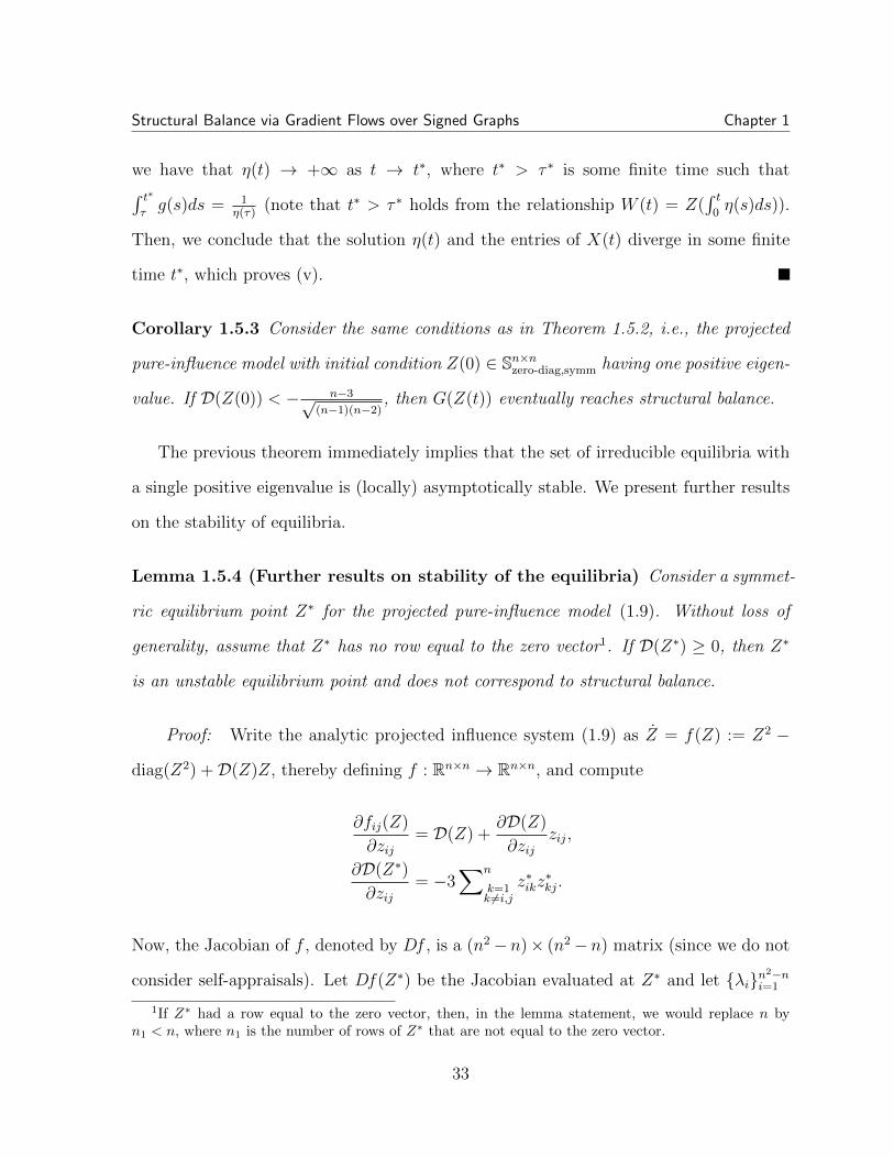
Corollary 1.5.3 Consider the same conditions as in Theorem 1.5.2, i.e., the projected
pure-influence model with initial condition Z(0) ∈ Sn×nzero-diag,symm having one positive eigen-
value. If D(Z(0)) < − n−3√(n−1)(n−2)
, then G(Z(t)) eventually reaches structural balance.
The previous theorem immediately implies that the set of irreducible equilibria with
a single positive eigenvalue is (locally) asymptotically stable. We present further results
on the stability of equilibria.
Lemma 1.5.4 (Further results on stability of the equilibria) Consider a symmet-
ric equilibrium point Z∗ for the projected pure-influence model (1.9). Without loss of
generality, assume that Z∗ has no row equal to the zero vector1. If D(Z∗) ≥ 0, then Z∗
is an unstable equilibrium point and does not correspond to structural balance.
Proof: Write the analytic projected influence system (1.9) as Z = f(Z) := Z2 −
diag(Z2) +D(Z)Z, thereby defining f : Rn×n → Rn×n, and compute
∂fij(Z)
∂zij= D(Z) +
∂D(Z)
∂zijzij,
∂D(Z∗)
∂zij= −3
∑n
k=1k 6=i,j
z∗ikz∗kj.
Now, the Jacobian of f , denoted by Df , is a (n2− n)× (n2− n) matrix (since we do not
consider self-appraisals). Let Df(Z∗) be the Jacobian evaluated at Z∗ and let λin2−ni=1
1If Z∗ had a row equal to the zero vector, then, in the lemma statement, we would replace n byn1 < n, where n1 is the number of rows of Z∗ that are not equal to the zero vector.
33

Structural Balance via Gradient Flows over Signed Graphs Chapter 1
be the set of its eigenvalues. Then, we compute
n2−n∑
i=1
λi = trace(Df(Z∗)) =n∑
i=1
∑n
j=1j 6=i
∂fij(Z∗)
∂zij
= (n2 − n)D(Z∗) + 3D(Z∗) = (n2 − n+ 3)D(Z∗).
Since n2 − n + 3 > 0 for n ≥ 3, we draw the following conclusions for D(Z∗) ≥ 0:
(i) Df(Z∗) contains at least one positive eigenvalue and so the equilibrium point Z∗ is
unstable; (ii) at least one triad in G(Z∗) is unbalanced and so Z∗ does not correspond
to structural balance.
1.6 Simulation results and conjectures
The generic convergence of trajectories to the minima of D (or, equivalently, the
convergence from almost all initial conditions) is an open problem. However, we present
strong numerical evidence that support such claim. We first remark that, from the proof
of Theorem 1.3.3, the projected pure-influence model (1.9) can be generalized over any
asymmetric matrix in Sn×nzero-diag by replacing D(Z) by − trace(Z>Z2) and this is the model
we will refer throughout this section.
A generic asymmetric initial condition X(0) for the pure-influence model (1.2) is a
matrix that is generated with each entry independently sampled from a uniform distribu-
tion with support [−100, 100], and its diagonal entries set to zero. A generic symmetric
initial condition is similarly constructed by only sampling the upper triangular entries
of the matrix. For the projected pure-influence model, we say Z(0) = X(0)‖X(0)‖F
is a
(non-)symmetric generic initial condition depending on how X(0) was generated. We
immediately see from the proof of Theorem 1.5.2, that Z(t) converges to social balance
if and only if X(t) converges to social balance. Indeed, given that X(t) diverges at some
34

Structural Balance via Gradient Flows over Signed Graphs Chapter 1
finite time t, we have Z(∞) = X(t−)‖X(t−)‖F
.
For a fixed network size n, we use a Monte Carlo method [162] to estimate the proba-
bility p of the event “under a generic asymmetric initial condition Z(0), Z(t) converges to
structural balance in finite time”. We estimate p by performing N independent simula-
tions (i.e., each simulation generates a new independent initial condition) and obtaining
the proportion pN , also known as the empirical probability, of times that the simula-
tion indeed had Z(t) converging to structural balance in finite time. For any accuracy
1−ε ∈ (0, 1) and confidence level 1−η ∈ (0, 1) we have that |pN−p| < ε with probability
greater than 1− η if the Chernoff bound N ≥ 12ε2
log 2η
is satisfied. For ε = η = 0.01, the
bound is satisfied by N = 27000. We performed the N = 27000 independent simulations
with n ∈ 5, 6, and found that pN = 1. Our observations let us conclude that for generic
asymmetric initial condition Z(0) and n ∈ 5, 6, with 99% confidence level, there is at
least 0.99 probability that Z(t) converges to structural balance in finite time.
Similarly, we performed the same Monte Carlo analysis for generic symmetric initial
conditions with n ∈ 3, 5, 6, 15, and found for that pN = 1 for all n. Therefore, we
conclude that for any symmetric generic initial condition Z(0) and n ∈ 3, 5, 6, 15, with
99% confidence level, there is at least 0.99 probability that Z(t) converges to structural
balance in finite time.
We report three more observations and then state a resulting conjecture. First, re-
markably, we found that all of our simulations (for any type of random initial condition)
that converged to structural balance in finite time, did it by converging to an equilib-
rium point having only one positive eigenvalue inside the set of scale-symmetric matrices,
which is a superset of the set of symmetric matrices (see Appendix 1.8.2). Second, we did
not perform experiments for larger sizes of n due to computational constraints. Third,
unfortunately, for n = 3, we did find randomly-generated asymmetric initial conditions
whose numerically-computed solutions do not converge to structural balance.
35

Structural Balance via Gradient Flows over Signed Graphs Chapter 1
Conjecture 1 (Convergence from generic initial conditions) Consider the pure-
influence model (1.2) with some initial condition X(0), and the projected pure-influence
model (1.9) with initial condition Z(0) = X(0)‖X(0)‖F
. Then,
(i) under generic asymmetric initial conditions, limt→+∞ Z(t) = Z∗ for a sufficiently
large n,
(ii) under generic symmetric initial conditions, limt→+∞ Z(t) = Z∗ for any n,
where Z∗ is scale-symmetric (and particularly symmetric for (ii)) corresponding to struc-
tural balance. Then, Z(t) reaches structural balance in finite time. Moreover, X(t)
reaches structural balance in finite time with same sign structure as Z∗, and also diverges
in finite time.
Similarly, we performed the same simulation analysis for the Ku lakowski et al. model
(1.4), which converges to structural balance if and only if the projected Ku lakowski
model (1.10) does. To generate a generic initial condition for this system, we generated
an n×n matrix with each entry independently sampled from a uniform distribution with
support [−100, 100], and then divide it by its Frobenius norm. We performed N = 27000
independent simulations with n ∈ 5, 6, and found that for generic initial condition
Z(0) and n = 5, only 16.94% converged to structural balance, and for n = 6, only 11.50%
converged to structural balance.
Also, for n = 3, not all simulations converged to structural balance. We remark that
not all of the networks for which the system converged and did not satisfy structural bal-
ance were complete, some of them were networks with only self-loops, e.g., Figure 2.3(a).
Similarly, we performed the same Monte Carlo analysis for symmetric initial conditions
with n ∈ 3, 5, 6, 15. Our results show that for symmetric generic initial condition,
Z(0) did not always converge to structural balance for n = 3, but, for n ∈ 5, 6, 15, with
36

Structural Balance via Gradient Flows over Signed Graphs Chapter 1
99% confidence level, there is at least 0.99 probability that Z(t) converges to structural
balance in finite time.
These Monte Carlo results are expected, since it has been formally proved that the
Ku lakowski et al. model converges to structural balance only under generic symmetric
initial conditions as n → ∞ [119] and negative results for asymmetric conditions are
given by [164].
See Figure 3.4 for a comparison of trajectories of the pure-influence model in both
generic and symmetric generic initial conditions. Figure 1.4 shows a comparison between
our projected pure-influence model, which does not consider self-appraisals, and the
projected influence model, which considers self-appraisals. Note how not considering
self-appraisals drastically changes the convergence time as well as the dynamic behavior
of the interpersonal appraisals.
(a) Projected pure-influence model (1.9) withgeneric asymmetric initial condition
0 5 10 15 20 25 30 35
t
-0.3
-0.2
-0.1
0
0.1
0.2
0.3
Z(t
)
(b) Projected pure-influence model (1.9) withgeneric symmetric initial condition
Figure 1.3: Convergence to structural balance for a network of size n = 10. We plotthe evolution of all the entries of Z(t).
37

Structural Balance via Gradient Flows over Signed Graphs Chapter 1
0 5 10 15
t
-0.5
-0.4
-0.3
-0.2
-0.1
0
0.1
0.2
0.3
0.4
Z(t)
(a) Projected influence model (1.10) withgeneric asymmetric initial condition
0 100 200 300 400 500 600 700
t
-1
-0.5
0
0.5
1
Z(t
)
(b) Projected pure-influence model (1.9) withgeneric asymmetric initial condition
Figure 1.4: Convergence comparison for a network of size n = 7 (a) with and (b)without the consideration of self-appraisals. We first generated an n × n randommatrix W with each entry independently sampled from a uniform distribution withsupport [−100, 100]. Then, for (a), we normalize this matrix to have unit Frobeniusnorm and used it as the initial condition. For (b), we set the diagonal entries of Wto zero and then normalize it to have unit Frobenius norm and use it as the initialcondition. In this example, (a) did not converged to structural balance, whereas (b)did. We plot the evolution of all the entries of the appraisal matrix.
1.7 Conclusion
We propose two new dynamic structural balance models that incorporates more psy-
chologically plausible assumptions than previous models in the literature, based on a
modification by a model proposed by Ku lakowski et al. We have established important
convergence properties for these models and also that, most importantly, they correspond
to gradient systems over an energy function that characterizes the violations of Heider’s
axioms for the symmetric case. We also expanded our results to a set of asymmetric
matrices called scale-symmetric. Numerical results illustrates that, under generic initial
conditions, our models converges to structural balance (for sufficiently large n) and thus
have better convergence properties than the previous model by Ku lakowski et al.
As future work, we propose to further study the general case of asymmetric (and non-
38

Structural Balance via Gradient Flows over Signed Graphs Chapter 1
0 5 10 15 20 25 30 35 40
t
-0.6
-0.4
-0.2
0
0.2
0.4
0.6
0.8
Z(t
)
(a) Projected influence model (1.10) with genericasymmetric initial condition
0 20 40 60 80
t
-0.5
0
0.5
1
Z(t)
(b) Projected pure-influence model (1.9)with generic asymmetric initial condition
Figure 1.5: Convergence comparison for a network of size n = 7 (a) with and (b)without the consideration of self-appraisals. The setting is the same one as in Fig-ure 1.4, but with a different random initial condition. (a) converged to a network withonly diagonal negative entries (all interpersonal appraisals go to zero), whereas (b)converged to structural balance.
scale-symmetric) equilibria and the convergence properties of our models under arbitrary
initial conditions. For example, numerical simulations of the projected pure-influence
model from generic (asymmetric) initial conditions illustrate how this system features
transient chaos before converging towards an equilibrium. Future work will focus on
models with a more sociologically justified transient behavior. Finally, one could study
the removal of the self-appraisals in other dynamical structural balance models, like the
homophily-based model by Traag el al. [164].
1.8 Appendix
1.8.1 Supporting results and proofs
Lemma 1.8.1 Let x(t) be the solution to x = f(x) from initial condition x(0), with
f being a continuously differentiable vector field. Let η be a positive continuous scalar
39

Structural Balance via Gradient Flows over Signed Graphs Chapter 1
function. Then, z(t) is the solution to z = η(t)f(z) with initial condition z(0) = x(0) if
and only if z(t) = x(∫ t
0η(s)ds).
Proof: Consider the time transformation t(t) =∫ t
0η(s)ds, which is well-defined since
it is continuous and monotonically increasing on t (recall that η(s) > 0 for s ∈ [0, t]),
with t = 0 if and only if t = 0. Now, from the chain rule, it follows that
dz
dt=dx(t)
dt
dt
dt= f(z)η(t), z(0) = x(0).
This finishes proof of the “if” part. The “only if” part follows from the uniqueness
theorem.
Proof: [Proof of Lemma 1.4.1] First, to prove that the set nSt(n, k), k ≤ n is a
submanifold of the compact Stiefel manifold, define the smooth map Φ : St(n, k) → Rn
by X 7→ (‖Xi∗‖22 , . . . , ‖Xn∗‖2
2)>, where Xi∗ is the ith row of X. Then, we have that
nSt(n, k) = Φ−1((k/n, . . . , k/n)>) and it is easy to prove the mapping Φ has constant
rank n. Thus, we use the Constant-Rank Level Set Theorem [102] to conclude our claim.
The properties of compactness and analyticity are immediate from the definition of the
set nSt(n, k), k ≤ n.
Now, notice that conditions ((i)) and ((ii)) from Definition 1.4.1 impose, in total,
k(k+1)2
+n constraints on kn independent variables, however, these constraints are linearly
dependent: one of them can be removed (for instance, if one requires condition (i) from
Definition 1.4.1, then suffices to constrain only sums of n−1 rows, whereas the remaining
sum automatically equals k/n)). Whenever k ≤ n and n ≥ 3, one has k(k+1)2
+n−1 < kn,
which implies that the set nSt(n, k) has the dimension (k − 1)n+ 1− k(k + 1)/2.
Statements (i) and (ii) are immediate. Now regarding (iii), it is obvious that each
row has norm√k/n if and only if V can be written as (1.16). Notice now the columns
are unit vectors if and only if∑n
m=1 cos2 αi = n/2 =∑n
m=1 sin2 αi, which in turn holds if
40

Structural Balance via Gradient Flows over Signed Graphs Chapter 1
and only if∑
m cos 2αm = 2∑
m cos2 αm−n = 0. Similarly, the columns are orthogonal if
and only if∑n
m=1 cosαi sinαi = 0 = 12
∑m sin 2αm. These two constraints are equivalent
to (1.17).
Proof: [Proof of Lemma 1.4.2] The case where α = β = 0 is trivial: Z = 0 and it
obviously can be decomposed as in (1.18) with p = q = 0. Notice that every eigenvalue of
Z = Z> corresponds to the eigenvalue λ2−2αλ of Z2−2αZ, and hence λ2−2αλ−β = 0.
Therefore, α2 + β ≥ 0 (otherwise, eigenvalues of Z would be complex). Furthermore,
α2 + β 6= 0 (otherwise, λ = α would be the only eigenvalue of Z of multiplicity n, and
one would have trace(Z) = αn, entailing that α = β = 0). Denoting ∆ =√α2 + β, the
matrix Z has two different eigenvalues α+ ∆ and α−∆, denote their multiplicities by k
and n− k. Then (α+ ∆)k + (α−∆)(n− k) = 0. Denoting q = ∆− α and p = 2∆ > 0,
one has (p− q)k − q(n− k) = 0 or, equivalently, pk = qn thus, q > 0.
Consider the orthonormal eigenvectors v1, . . . , vk, corresponding to the eigenvalue
p− q = α+∆ and orthonormal eigenvectors w1, . . . , wn−k, corresponding to −q = α−∆.
The sequence v1, . . . , vk, w1, . . . , wn−k constitutes an orthonormal basis of eigenvectors
for the operator Z. Stacking the columns vi and wi, one obtains n× k and n× (n− k)
matrices V = (v1, . . . , vk), W = (w1, . . . , wn−k). The matrix [V,W ] is orthonormal
and diagonalizes Z, that is, Z[V,W ] = [V,W ]
(p− q)Ik 0
0 −qIn−k
and thus Z = (p −
q)V V > − qWW>. Since V V > + WW> = In, Z is decomposed as (1.18). It remains to
notice that V >V = Ik by definition of the orthonormal basis and diag(V V >) = (q/p)In =
(k/n)In since, by (1.18), diag(Z) = 0n×n. To finish the proof, notice that p − 2q = 2α
and β = ∆2 − α2 = (∆− α)(∆ + α) = q(p− q).
Proof: [Proof of Corollary 1.4.3] Let f(z) = z2 − 2αz, z ∈ C. It suffices to
show that, if f(Z) = diag(β1In1 , . . . , βsIns), then Z = diag(Z1, . . . , Zs), where f(Zi) =
βiIni . This statement will be proved for any analytic function f(z). It is well known
41

Structural Balance via Gradient Flows over Signed Graphs Chapter 1
that the spectrum of f(Z) consists of all points f(λ), where λ is an eigenvalue of Z.
Consider the set of eigenvalues of Z that belong to f−1(βi) and let Xi be the sum of
corresponding eigenspaces. Then Xi is invariant under the operator Z, and Rn = ⊕si=1Xi(the sum is orthogonal). Also, f(Z)x = βix for any x ∈ Xi. For any basis vector
er = (0, . . . , 1, . . . , 0)> consider the decomposition er = ⊕si=1eir, e
ir ∈ Xi. Then Zer =
⊕si=1Zeir, Ze
ir ∈ Xi and f(Z)er = ⊕si=1f(Z)eir = ⊕si=1βie
ir. Suppose that 1 ≤ r ≤ n1.
Then f(Z)er = β1er. Since β1, . . . , βs are pairwise different, we have er = e1r and e2
r =
. . . = esr = 0. Similarly, for n1 + n2 + . . .+ nj−1 + 1 ≤ r ≤ n1 + n2 + . . .+ nj−1 + nj one
has er = ejr (j = 2, . . . , s).
In other words, each Xi contains ni basis vectors er, where n1 + n2 + . . .+ ni−1 + 1 ≤
r ≤ n1 + n2 + . . . + ni−1 + ni and thus dimXi ≥ ni. Recalling that n1 + . . . + ns = n,
one shows that dimXi = ni ∀i and thus Xi is spanned by the corresponding basis vectors.
Since Xi is invariant under Z, Z = diag(Z1, . . . , Zs), where the block Zi has dimension
ni × ni. Obviously, f(Zi) = βiIni . The statement of Corollary is now immediate from
Lemma 1.4.2.
Proof: [Proof of Theorem 1.4.5] We prove the necessity first. Denoting 2α =
−D(Z). By assumption, Z2 − 2αZ is diagonal. Statements (i) and (ii) follow from
Corollary 1.4.3, entailing also that pi, qi can be represented as (1.23) with some βi. Since
Z2i = 2αZi + βiIni and diag(Zi) = 0ni×ni , one has traceZ2
i = βini, therefore
∑s
i=1βini = trace(Z2) = 1. (1.29)
Recall also that for each i one has piki = qini or, equivalently,
2kini
=
√α2 + βi − α√α2 + βi
= 1− α√α2 + βi
∀i : pi, qi 6= 0.
42

Structural Balance via Gradient Flows over Signed Graphs Chapter 1
(if α = 0, one always has pi, qi 6= 0, otherwise it is possible that βi = 0 and then Zi = 0).
This implies condition 3 (ε = signα) and allows to determine α, βi. In the case where
ε 6= 0 notice that ni − 2ki 6= 0 for any i such that Zi 6= 0. Thus
βi + α2
α2=
n2i
(ni − 2ki)2⇐⇒ βi = α2 4niki − 4k2
i
(ni − 2ki)2.
In view of (1.29), one obtains that
α = ε
∑
i:Zi 6=0ni×ni
4kini(ni − ki)(ni − 2ki)2
−1/2
,
which entails (1.24). In the case of α = 0, one has pi = 2√βi, qi =
√βi for any i,
and (1.29) implies that∑
i q2i ni = 1. This finishes the proof of statement (iv).
The proof of sufficiency is similar. For any i such that Zi 6= 0, the coefficients pi, qi
have the form (1.23) (if ε 6= 0, this is implied by (iv)a, otherwise we choose α = 0 and
βi = q2i = p2
i /4). Therefore, we have Z2i − 2αZi = βiZi and, in particular, Z2 − 2αZ
is diagonal. A straightforward computation shows that piki = qini and thus diag(Zi) =
0ni×ni ∀i, in particular, diag(Z) = 0n×n. Also, diag(Z2i ) = βiIni , and statement (iv)
now implies that traceZ2 = 1. It remains to notice that Z3i = 2αZ2
i + βiZi, and hence
trace(Z3i ) = 2αβini. Hence, D(Z) = − trace(Z3) = −2α, Z2 + D(Z)Z is a diagonal
matrix, and Z is an equilibrium (1.14).
43

Structural Balance via Gradient Flows over Signed Graphs Chapter 1
1.8.2 Scale-symmetric matrices
We now generalize our results for symmetric appraisal networks to a class of asym-
metric matrices. We define the sets of scale-symmetric matrices
Rn×nzero-diag,dss = A ∈ Rn×n
zero-diag|there exists γ 0n such that
A diag(γ) = (A diag(γ))>,
Sn×nzero-diag,dss = Sn×nzero-diag ∩Rn×nzero-diag,dss.
Note that Sn×nzero-diag,dss ⊃ Sn×nzero-diag,symm and
Sn×nzero-diag,dss =⋃
γ0n
Sn×nzero-diag,dss(γ),
Sn×nzero-diag,dss(γ) =A ∈ Sn×nzero-diag | A diag(γ) = (A diag(γ))>
.
.
Lemma 1.8.2 Consider any γ 0n and some matrix A ∈ Rn×n such that A diag(γ) =
diag(γ)A>. Then,
(i) A has real eigenvalues and it is diagonalizable,
(ii) trace(A2) = 0 if and only if A = 0.
Proof: Since A diag(γ) is symmetric, then A′ = diag(γ)−1/2A diag(γ)1/2 is also
symmetric and thus has real eigenvalues and its eigenvectors form an orthogonal basis.
Now, let (λ, v) be an eigenpair for A′. Then, by defining u = diag(γ)1/2v, we observe
that Au = λu, and so (λ, diag(γ)v) is an eigenpair for A. Hence the eigenvectors of A
form a basis, and thus A is diagonizable. This proves (i).
Observe that
A = diag(γ)A> diag(γ)−1.
44

Structural Balance via Gradient Flows over Signed Graphs Chapter 1
Then, trace(A2) = trace(A diag(γ)A> diag(γ)−1). From simple algebraic operations, it
can be found that trace(A2) =∑n
i=1
∑nj=1
γjγia2ij. Since γi
γj> 0, trace(A2) = 0 if and only
if A = 0. This proves (ii).
In view of Lemma 1.8.2, a matrix A is scale-symmetric if and only if A = D−1AsD,
where D > 0 is a positive diagonal matrix (in Lemma 1.8.2, D = diag(γ−1/2) for some
γ 0n) and As a symmetric matrix.
Recall the invariance property of the pure-influence model (1.2): if X(0) = X(0)>,
then X(t) = X(t)> for all t > 0. We are now ready to provide a more general version
of this property: If D > 0 is a diagonal matrix and X(t) is a solution, then DX(t)D−1
is also a solution. For this reason, if X(0) = DXs(0)D−1 is a scale-symmetric matrix
with some Xs(0) = Xs(0)>, then the solution X(t) = DXs(t)D−1 is scale-symmetric.
A similar result holds for the projected pure-influence model (1.9). Indeed, all of the
theoretical results obtained in this paper for symmetric appraisal matrices, can be gen-
eralized to scale-symmetric appraisal matrices. For example, if X(0) ∈ Rn×nzero-diag,dss
(Z(0) ∈ Sn×nzero-diag,dss) then t 7→ D(X(t)) (t 7→ D(Z(t))) is monotonically nondecreasing in
Rn×nzero-diag,dss (Sn×nzero-diag,dss).
45

Chapter 2
Polarization and Fluctuations in
Signed Social Networks
2.1 Introduction
There have been various opinion dynamics models in the literature [5, 144]. Opinions
can be modeled as real numbers taking values in the closed interval [0, 1], where 0 means
an agent completely disagrees with a particular issue, and 1 that she completely agrees.
One important question to answer is how the evolution and final distribution of opinions
in a social network depend on the underlying network’s topology and of the (positive)
influence structure among the individuals. More recently, signed graphs were introduced
into the opinion dynamics literature. Signed graphs represent a natural way to model pos-
itive and negative relationships among individuals. For example, a sociological relevant
concept is structural balance, in which the members of a social network can either have
only positive relationships or be divided in two factions in which members of the same
faction have positive relationships but negative ones with members of the other faction.
The seminal work by Altafini [7] proposed a continuous time model over a signed graph
46

Polarization and Fluctuations in Signed Social Networks Chapter 2
where the opinions can take any real value. It is shown that when the underlying graph
satisfies structural balance (and assuming that it is strongly connected), the opinions
converge to bipartite consensus and polarize, i.e., all opinions have the same absolute
value with their signs indicating which agents belong to the same faction (if there is one
faction, all opinions have the same sign). A discrete-time signed opinion model which is
a counterpart of the Altafini model has also been proposed [78, 124], in which bipartite
consensus is also attained under structural balance. These two models have initiated a lot
of research in the field of signed opinion dynamics, and are, arguably, the most popular
models in the literature. Extensions of these models and further analysis have been done
in the literature, as can be noted in the recent work [108] and the references therein.
Note, however, that both Altafini models and their extensions present an unrealistic
opinion vanishing behavior (i.e., the opinions converge to zero) whenever the property
of structural balance is lost in the underlying social network, with the underlying graph
still being strongly connected.
Another class of models in opinions dynamics was proposed by Li et al. [104] and is
based on an extension of the voter model to signed graphs. In this model, individuals
initially take binary opinion values (e.g., 0 and 1). Then, at each subsequent time step,
an individual is selected according to some process and updates her opinions by copying
the same or the opposite opinion of one of her neighbors according to the sign of their
relationship. By design, opinions cannot vanish under generic signed networks; however,
the opinion values are simply discrete. Whenever the graph satisfies structural balance,
they showed that the opinions polarize: one faction takes one value, while the other
faction takes the remaining one. Recently, Lin et al. [107] proposed a model which can
be regarded as an extension to the one from Li et al. In this model, opinions can take
m different discrete values from a set S. Then, an individual will copy the same opinion
from a positive neighbor, but when facing a negative one, will randomly select an opinion
47

Polarization and Fluctuations in Signed Social Networks Chapter 2
different from that neighbor from the set S.
In this paper, we propose a novel opinion model over signed graphs. We assume
that the opinions are real numbers taking value in a closed interval and each edge of the
graph indicates the friendly or antagonistic relationship between two individuals. Our
model is inspired by the boomerang effect studied in social psychology [46, 35, 1], which
aims to explain why in some situations where two individuals engage in communication,
they may not end up being in a better agreement but rather their attitudes become
more dissentive, i.e., their opinions do not go in the intended direction (e.g., consensus
or agreement) but in the opposite direction (e.g., polarization). The early work [84] sug-
gested that this phenomenon can be explained by “the relative distance between subjects’
attitudes and position of communication”. Our model is motivated by the empirical ob-
servations in the social sciences (e.g., from the study of interpersonal attraction [17]) that
two friendly agents will be closer in their attitudes and perspectives than two unfriendly
agents. Specifically, we make the following assumption: whenever two agents who have
a positive relationship interact, they are more agreeable and their opinions will become
closer or even be in consensus, i.e., the opinion changes in the intended direction. On the
other hand, whenever two agents with a negative relationship interact, the differences
in their opinions will be more polarized after the interaction because of their increas-
ing disagreement, i.e., the opinion changes in the opposite direction. Our opinion model
captures such behavior mathematically, and we call it the affine boomerang model. Math-
ematically, our proposed model is an affine model, which makes it remarkably simple,
and its dynamics are self-explanatory. Besides a linear model like the discrete Altafini
model, this is, arguably, the next simplest model structurally.
Our second contribution is a formal analysis of our proposed model: under certain
conditions on the sign structures of the network that corresponds to structural balance,
our model expresses opinion polarization, i.e., the opinions of two groups converge to
48

Polarization and Fluctuations in Signed Social Networks Chapter 2
opposite extreme values of the closed interval.
Finally, it is important to compare our model and the aforementioned models in the
literature. Our model has the property that opinions do not necessarily vanish whenever
the graph is not balanced, but, for example, can continue fluctuating inside the closed
interval. The vanishing behavior, which we mentioned happens in both types of Altafini
models and their extensions, has been interpreted as if the agents in the network become
neutral or indifferent towards a specific topic. In the case of three antagonistic groups
in a connected network, this would mean that all groups will end up having a zero
valued opinion, i.e., they will have consensus on not having an opinion. This might be
difficult to interpret. Instead, our proposed model predicts that two groups will polarize
their opinions and the third one will continue fluctuating its opinions since its members
observe people they dislike having opposite opinions. Thus, this third group does not
settle down to a definite opinion and its members are persistently disagreeing with each
other. This is, arguably, more intuitive since individuals of a social network can always
hold an opinion, independently of whether their network is balanced or not. Moreover if
we have an unbalanced network that differs from a balanced one in just the sign of one
edge, it is not clear why that would drive the whole social network towards an indifferent
opinion. Instead, our model suggests that opinions may fluctuate around extreme values
of opinion, which is more intuitive since the underlying social network is approximately
balanced.
2.2 The model
A signed graph G is an undirected graph with signed edges, i.e., with edge weights
equal to either +1 or −1. Let E = E+ ∪E− be the edge set of G, where E+ is the set of
positive edges and E− the set of negative edges. G is complete when there exists an edge
49

Polarization and Fluctuations in Signed Social Networks Chapter 2
between any pair of vertices. A path from vertex i to j in G is a sequence of edges that
connect a sequence of distinct vertices starting from i and finishing at j. A connected
component is any subgraph such that all of its vertices are connected to each other by
paths, but they are not connected to any other vertex of G. G is connected whenever it
has only one connected component. The abbreviation i.o. stands for infinitely often.
We model the structure of a social network composed by agents as a graph. Then,
throughout the paper, we use the words graph and network interchangeably, as well as the
terms vertex and agent. Each agent in the network holds an opinion about a particular
statement of a discussion topic, and her opinion describes how much she agrees with it.
An agent i has an opinion xi ∈ [omin, omax]: xi = omax whenever i completely agrees with
the statement being discussed, and xi = omin whenever she completely disagrees with it.
The opinion vector x ∈ [omin, omax]n has in its ith entry the opinion xi of agent i.
Definition 2.2.1 (Sign arrangement property) Given a connected signed graph G =
(1, . . . , n, E+ ∪E−) with n ≥ 3, let G+ = (1, . . . , n, E+). For k ∈ N, we say that G
satisfies the k-sign arrangement property if
(i) G+ has k ≥ 1 connected components, and
(ii) each negative edge connects vertices belonging to different connected components of
G+.
If this property holds, then each connected component of G+ is a faction.
Based on the works [38, 54] in the sociological literature, we definite the notion of
structural and clustering balance for connected graphs.
Definition 2.2.2 (Structural and clustering balance) Consider a connected signed
graph G with n ≥ 3. Assume the vertices of G can be partitioned in m groups such that
50

Polarization and Fluctuations in Signed Social Networks Chapter 2
each positive edge joins two vertices from the same group and each negative edge joins
vertices from different groups. We say that G satisfies
(i) structural balance if m ≤ 2, and
(ii) clustering balance if m ≥ 3.
The following result follows immediately from the previous definitions.
Lemma 2.2.1 Let G be a complete signed graph. G satisfies the k-sign arrangement if
and only if it satisfies structural balance when k ≤ 2 or clustering balance when k ≥ 3.
Note that a signed graph satisfying the k-sign arrangement property does not need
to be complete.
Definition 2.2.3 (Affine boomerang model) Let G = (1, . . . , n, E+ ∪E−) be a signed
graph. Assume that each agent has an initial opinion xi(0) ∈ [omin, omax], omin < omax,
and a self-weight ai ∈ (0, 1). At each time step t ∈ Z≥0, select randomly an edge of G;
assume each edge i, j has a time-invariant positive selection probability pij. Update the
opinions of the two agents i and j according to:
xi(t+ 1) =
aixi(t) + (1− ai)xj(t), if i, j ∈ E+,
aixi(t) + (1− ai)omin,
if i, j ∈ E− and xi(t) < xj(t),
aixi(t) + (1− ai)omax,
if i, j ∈ E− and xi(t) ≥ xj(t),
(2.1)
and similarly for agent j.
The following remarks interpret and elaborate on the various features of the model.
51

Polarization and Fluctuations in Signed Social Networks Chapter 2
Remark 2.2.2 (Bounded evolution) In our model, opinions take values on an ar-
bitrary closed interval [omin, omax]. From a sociological (and intuitive) point of view, it
is plausible to have bounded opinions since there is no clear interpretation of diverging
opinions. Indeed, bounded opinions are present throughout the literature on opinion dy-
namics. The case omin = −θ and omax = θ, for θ > 0, is characteristic in the literature
on bipartite consensus (e.g., [7, 156]), and the case omin = 0 and omax = 1 is charac-
teric in the literature of opinion dynamics over graphs with positive weights (e.g., [5]) or
bounded-confidence models (e.g., [39]).
Remark 2.2.3 (Asynchronous updating) Our model features asynchronous updat-
ing of the opinions since only two opinions are updated simultaneously and independently
per time step, instead of all opinions at once (which would be synchronous updating).
This type of updating has been studied in other previous opinion models, e.g., in the
Deffuant-Weisbuch model [39] and in the gossip model [31]. A classic strategy is to
assign homogeneous selection probability to each edge in the graph.
Remark 2.2.4 (Magnitude of the boomerang effect) Assume i and j are two agents
with an antagonistic relationship and, without loss of generality, assume xi(t) > xj(t).
As stated in the last case of equation (4.3), when i and j interact, the opinion xi(t + 1)
jumps towards the extreme opinion omax and does so independently of the opinion differ-
ence dij(t) = |xi(t)− xj(t)|. Note that this is a simplifying assumption in the sense that
the jump magnitude (i.e., the magnitude of the boomerang effect) could be assumed to
be directly proportionally to dij(t), inversely proportional to dij(t), or , more generally,
a positive function of dij(t) ensuring boundedness of the evolutions. This simplifying
assumption is justified because, to the best of our knowledge, no empirical evidence or
psychological theory is available about the jump magnitude or about whether the magni-
tude should even depend upon dij at all. In this sense, our independence assumption is
52

Polarization and Fluctuations in Signed Social Networks Chapter 2
arguably the simplest (and therefore preferrable) model.
2.3 Model analysis
In this section, we first introduce the two main theoretical results from our paper,
namely, that the affine boomerang model can explain, given certain conditions on the
underlying social network, both the polarization of opinions and their persistent fluc-
tuations. Additionally, we present some numerical results on how opinions attempt to
polarize when these conditions on the underlying social network are relaxed.
2.3.1 Theoretical results
Theorem 2.3.1 (Consensus and polarization in signed graphs) Consider a net-
work satisfying the k-sign arrangement property. Consider the evolution of the affine
boomerang model (4.3) with initial opinion vector x(0) ∈ [omin, omax]n. Then
(i) Consensus: if k = 1, then, with probability one, limt→∞ x(t) = c1n, where c is a
random convex combination of the entries of x(0).
(ii) Polarization: if k = 2, then, with probability one, limt→∞ xi(t) = omin for each
agent i of one of the two factions and limt→∞ xj(t) = omax for each j of the other
faction.
Proof: Formally, at any time step, the selected edge is a discrete random variable
over some probability space (Ω′,F ′,P′) with Ω′ being the set of all edges on the graph, F ′
the power set, and P′[i, j] = pij. Let ω(t) be the random edge selected at time t, then,
the collection of random variables ω(t) | t ∈ Z≥0 forms a stochastic process of an in-
dependent sequence of random variables. Then, an adequate probability space (Ω,F ,P)
53

Polarization and Fluctuations in Signed Social Networks Chapter 2
can be constructed with Ω =∏
t∈Z≥0Ω′, F being the product of σ-algebras F ′ over
t ∈ Z≥0, and P being the product probability measure∏
t∈Z≥0P′. Therefore, given the se-
quence of edges s(t)t∈S with some finite set S ⊂ Z≥0, P[ω ∈ Ω | ω(t) = s(t), t ∈ S] =∏
t∈S P′[s(t)].
We start by considering the case k = 1. In this case, the model is a linear system
of the form x(t + 1) = W (t)x(t), where W (t) is a random matrix that takes, at each
time step, the value Wij = In×n − (1 − ai)ei(ei − ej)> − (1 − aj)ej(ej − ei)> whenever
the edge i, j is selected to be updated with probability pij (here, ei is the ith column
of the identity matrix In×n). With probability one, W (t) is a row stochastic matrix
with a strictly positive diagonal for any t; moreover W (t) is independent and identically
distributed for any t. Thus, E[W (t)] (with respect to P′) is a row stochastic matrix
that, when interpreted as an adjacency matrix, corresponds to a connected undirected
network. Under these assumptions, [32, Theorem 13.1] implies the first statement of the
theorem.
Now we prove the case k = 2. For any opinion vector x ∈ [omin, omax]n, we define the
variable Z : [omin, omax]n → 1, 2 as
(C1) Z(x) = 1 when there is no value τ > 0 such that one faction has all of its opinions
above τ and the other faction has them equal or below it;
(C2) Z(x) = 2 when there exists a value τ > 0 such that one faction has all of its
opinions above τ and the other faction has them equal or below it.
Clearly, Z exhausts all possible situations for the values of the opinion vector x, and,
moreover, induces a partition over the set [omin, omax]n: [omin, omax]n = ∪2m=1Z
−1(m) and
Z−1(1) ∩ Z−1(2) = ∅.
Now, let us remark that, from the random selection process of the edges, it immedi-
ately follows that x(t)t>0 is a random process over the probability space (Ω,F ,P); and,
54

Polarization and Fluctuations in Signed Social Networks Chapter 2
moreover, it is a Markov process, i.e., P[x(t) ∈ Z−1(m) |x(t− 1) = ct−1, . . . , x(0) = co] =
P[x(t) ∈ Z−1(m) |x(t − 1) = ct−1] for any m ∈ 1, 2. Observe that, with probability
one, x(t) ∈ [omin, omax]n for any t since x(0) ∈ [omin, omax]n.
Now, assume that x(t) ∈ Z−1(2) for some t < ∞. Let F1 be the faction such that
xi(t) ≤ τ for any i ∈ F1; and F2 the one such that xi(t) > τ for any i ∈ F2. Let
θF1(t) = maxi∈F1 xi(t) and θF2(t) = mini∈F2 xi(t). If at t + 1 some i ∈ F1 and j ∈ F2
are selected, we have that xi(t + 1) < xi(t) and xj(t + 1) > xj(t). On the other hand,
if at t + 1 both i and j belong to the same faction with xi(t) ≤ xj(t), we have that
xi(t) ≤ xi(t+ 1), xj(t+ 1) ≤ xj(t), with equality if and only if xi(t) = xj(t). From these
two observations it is easy to show that θF1(t + 1) ≤ θF1(t) with probability one; i.e.,
θF1(s)s≥t is a non-decreasing sequence which is lower bounded by omin. This implies
convergence of θF1(s)s≥t to some lower bound cmin with probability one. Now, for any
ε > 0 and t∗ ≥ t, there exists some finite T > 0 such that if the sequence of edges
(θF1(s), k(s))t∗+Ts=t∗ with k(s) ∈ F2 for t∗ ≤ s ≤ t∗ + T is selected, then |θF1(t∗ + T ) −
omin| < ε. Such sequence has a positive probability of being selected sequentially by the
affine boomerang model for any t∗, from which it follows that cmin = omin. Therefore,
there is polarization for any i ∈ F1 towards omin. A similar reasoning leads to the proof
that θF2(s)s≥t has an analogous increasing monotonic behavior and thus that there is
polarization for i ∈ F2 towards omax with probability one. In conclusion, if x(t) ∈ Z−1(2)
for t ≥ 0, then polarization occurs with probability one and we say that Z−1(2) is an
absorbing set since the opinion vector cannot escape from it once it enters this set.
Therefore, to finish the proof of the theorem, we only need to prove that, given
x(t) ∈ Z−1(1) at any time t, there always exists (with probability one) a finite se-
quence of edges such that eventually x(t∗) ∈ Z−1(2) for some t < t∗ < ∞. Then, since
any finite sequence of edges has positive probability of being selected sequentially by
the affine boomerang model and Z−1(2) is an absorbing set, it follows that P[x(t) ∈55

Polarization and Fluctuations in Signed Social Networks Chapter 2
Z−1(1) i.o. |x(0) ∈ Z−1(1)] = 0; and this finishes the proof for item (ii) of the theorem.
Therefore, it suffices to prove that P[x(t + T ) ∈ Z−1(2) for some T > 0 |x(t) = xo] = 1
for any xo ∈ Z−1(1). So, let us fix any xo ∈ Z−1(1). Let T1→2(t) = inft∗ > t : x(t∗) ∈
Z−1(2)|x(t) = xo be the first time, after starting in xo ∈ Z−1(1) at time t, at which the
opinion vector enters the set Z−1(2). If we show that P[T1→2(t) <∞] = 1 for any t, then
we have finished the proof.
By the Markov property, we only need to show that P[T1→2(0) < ∞] = 1. We
start by noticing that, by the finite-time proximity property (Lemma 2.5.1), there exists
a sequence of edges s(0), . . . , s(τ − 1) for some τ > 0 such that x(τ) ∈ Z−1(2). Let
γo := mini,j∈E pij. Then,
P[x(τ) ∈ Z−1(2)|x(0) = xo] ≥ P[ω(0) = s(0)|x(0) = xo]
× P[ω(1) = s(1) |x(0) = xo, ω(0) = s(0)] . . .
× P[ω(τ − 1) = s(τ − 1) |
x(0) = xo, ω(`) = s(`) for ` ∈ [0, τ − 2]]
= P′[s(0)]P′[s(1)] . . .P′[s(τ − 1)]
≥ (γo)τ ,
(2.2)
where the first inequality comes from a repetitive application of the conditional probabil-
ity and the following equality comes from the independence of the underlying stochastic
process. Let Γ > 0 be any integer and A` = x(t) /∈ Z−1(2), t ∈ [`, ` + τ ], then
P[A0|x(0) = xo] ≤ 1−γτo . Likewise, in a way similar to how we obtained expression (2.2),
56

Polarization and Fluctuations in Signed Social Networks Chapter 2
we compute
P[T1→2(0) ≥ (τ + 1)Γ] = P[x(t) /∈ Z−1(2), t ∈ [0, (τ + 1)Γ− 1]|x(0) = xo]
= P[∩Γ−1`=0A`(τ+1)|x(0) = xo]
= P[A0|x(0) = xo]
×Γ−1∏
`=1
P[A`(τ+1)|x(0) = xo,∩0≤`′≤`A`′(τ+1)]
≤ (1− γτo )Γ =: γΓ.
Now, we observe that∑∞
t=1 P[T1→2(0) ≥ (τ + 1)t] ≤ ∑∞t=1 γt = γ
1−γ < ∞ because of
geometric series since 0 < γ < 1. Then, by the first Borel-Cantelli lemma, we conclude
that P[T1→2(0) <∞] = 1. This concludes the proof.
A consequence of Theorem 2.3.1 is that a complete social network that satisfies struc-
tural balance with two factions ends up having its agents with totally opposite opinions.
This agrees with the intuitive result that antagonistic groups are expected to develop
polarized opinions, as shown by other models in the literature [104, 108]. Also, as ex-
pected, if there are no negative relationships between the agents (i.e., there is only one
faction), all agents reach consensus. Finally, we remark that, in our model, since the
opinions converge to omin and omax in the case of polarization, the agents’ final opinions
can be more extreme than the most extreme initial opinions. This phenomenon does not
arise in models proposed in the literature on bipartite consensus and based on weighted
averaging of opinions (e.g., in the Altafini model).
Lemma 2.3.2 (Fluctuations) Consider a network satisfying the k-sign arrangement
property with k ≥ 3 factions F1, . . . , Fk and such that there exists at least one negative
edge between any pair of factions. Consider the boomerang opinion dynamics model (4.3)
with xi(0) = omin for any i ∈ F1, xi(0) = omax for any i ∈ F2, and xi(0) ∈ (omin, omax)
57

Polarization and Fluctuations in Signed Social Networks Chapter 2
for any i ∈ Fk, k ≥ 3. Then, for any 0 < ε < (omax − omin)/2 and any i ∈ Fk, k ≥ 3,
P[xi(t) ∈ (omin, omin + ε) ∪ (omax − ε, omax) i.o.] = 1.
Proof: Note that xi(t) ∈ (omin, omax) for any t ≥ 0 and any i ∈ Fk, k ≥ 3,
with probability one. Pick a positive ε < (omax − omin)/2 and define the intervals A`ε =
(omin, omin + ε), Auε = (omax− ε, omax) and Acε = [omin + ε, omax− ε]. Note that these three
intervals are non-empty and form a partition of (omin, omax).
Now, take any i ∈ Fk, k ≥ 3. First, define the random stopping times τc→`(t) =
inft∗ > t |xi(t∗) ∈ A`ε|xi(t) ∈ Acε, τ`→u(t) = inft∗ > t |xi(t∗) ∈ Auε |xi(t) ∈ A`ε and
τu→`(t) = inft∗ > t |x(t∗) ∈ A`ε|xi(t) ∈ Auε . Note that, if the pair i, j is chosen, then
the opinion of i is always pushed towards omax if j ∈ F1, and always pushed towards
omin if j ∈ F2 (this follows from the fact that for any k ∈ F1 ∪ F2, xk(t) = xk(0) for
all t ≥ 0 with probability one). Then, following a reasoning similar to the one adopted
in the proof of Theorem 2.3.1, we conclude that P[τc→`(t) < ∞] = P[τ`→u(t) < ∞] =
P[τu→`(0) <∞] = 1 for any t ≥ 0, from which the result follows.
Note that the conditions for the underlying signed network in this lemma are imme-
diately satisfied if the network is complete and satisfies clustering balance. This lemma
is interpreted as follows. Assume there are multiple antagonistic groups of people such
that for any two groups there exist two members that can communicate with each other.
Additionally, assume that only two groups are already polarized in the opinion spectrum
with the rest having opinions at intermediate values (i.e., mathematically, in the interval
(omin, omax)). Then, these non-polarized groups will have their opinions always fluctu-
ating at intermediate values, i.e., their opinions do not polarize or reach consensus at
some specific value. Intuitively, since the boomerang effect is persistent on the agents
with intermediate values, these agents cannot settle on a definite opinion since they con-
58

Polarization and Fluctuations in Signed Social Networks Chapter 2
tinue to interact with antagonistic agents on both ends of the spectrum. This behavior
of opinion fluctuation has been observed in other models in the presence of stubborn
agents who forbid the consensus of opinions among the agents [4]. Our work is the first
one to propose a persistent fluctuating behavior based on the structure of friendly and
antagonistic relationships in a social network.
2.3.2 Numerical results
For a complete graph satisfying structural balance, which is a particular case satisfying
the conditions of Theorem 2.3.1, Figure 3.4 shows some example evolutions for self-
weights ai = a ∈ (0, 1) for any agent i. We observed that, in general, the larger the
self-weights, the more time the polarization process takes.
Figure 2.2 shows examples where the underlying signed network has three factions.
Remarkably, under generic initial conditions (which are weaker initial conditions than
the ones in Corollary 2.3.2), two factions tend to polarize and the opinions of the third
one show persistent fluctuations.
Finally, we provide numerical evidence of the behavior under networks that are the
result of perturbations on balanced networks. Consider the situation where a complete
and balanced social network with two antagonistic factions is randomly perturbed by
flipping the sign of some of its edges. Intuitively, for small perturbations, we would
expect that opinions, though not being able to perfectly polarize, would still “attempt”
to be in such a state and fluctuate near extreme values. Figure 2.3 shows some examples
confirming this phenomenon.
59

Polarization and Fluctuations in Signed Social Networks Chapter 2
0<latexit sha1_base64="(null)">(null)</latexit><latexit sha1_base64="(null)">(null)</latexit><latexit sha1_base64="(null)">(null)</latexit><latexit sha1_base64="(null)">(null)</latexit>
200<latexit sha1_base64="(null)">(null)</latexit><latexit sha1_base64="(null)">(null)</latexit><latexit sha1_base64="(null)">(null)</latexit><latexit sha1_base64="(null)">(null)</latexit>
t<latexit sha1_base64="(null)">(null)</latexit><latexit sha1_base64="(null)">(null)</latexit><latexit sha1_base64="(null)">(null)</latexit><latexit sha1_base64="(null)">(null)</latexit>
400<latexit sha1_base64="(null)">(null)</latexit><latexit sha1_base64="(null)">(null)</latexit><latexit sha1_base64="(null)">(null)</latexit><latexit sha1_base64="(null)">(null)</latexit>
0<latexit sha1_base64="(null)">(null)</latexit><latexit sha1_base64="(null)">(null)</latexit><latexit sha1_base64="(null)">(null)</latexit><latexit sha1_base64="(null)">(null)</latexit>
1<latexit sha1_base64="(null)">(null)</latexit><latexit sha1_base64="(null)">(null)</latexit><latexit sha1_base64="(null)">(null)</latexit><latexit sha1_base64="(null)">(null)</latexit>
.5<latexit sha1_base64="(null)">(null)</latexit><latexit sha1_base64="(null)">(null)</latexit><latexit sha1_base64="(null)">(null)</latexit><latexit sha1_base64="(null)">(null)</latexit>
(a) a = 0.25
0<latexit sha1_base64="(null)">(null)</latexit><latexit sha1_base64="(null)">(null)</latexit><latexit sha1_base64="(null)">(null)</latexit><latexit sha1_base64="(null)">(null)</latexit>
200<latexit sha1_base64="(null)">(null)</latexit><latexit sha1_base64="(null)">(null)</latexit><latexit sha1_base64="(null)">(null)</latexit><latexit sha1_base64="(null)">(null)</latexit>
t<latexit sha1_base64="(null)">(null)</latexit><latexit sha1_base64="(null)">(null)</latexit><latexit sha1_base64="(null)">(null)</latexit><latexit sha1_base64="(null)">(null)</latexit>
400<latexit sha1_base64="(null)">(null)</latexit><latexit sha1_base64="(null)">(null)</latexit><latexit sha1_base64="(null)">(null)</latexit><latexit sha1_base64="(null)">(null)</latexit>
0<latexit sha1_base64="(null)">(null)</latexit><latexit sha1_base64="(null)">(null)</latexit><latexit sha1_base64="(null)">(null)</latexit><latexit sha1_base64="(null)">(null)</latexit>
1<latexit sha1_base64="(null)">(null)</latexit><latexit sha1_base64="(null)">(null)</latexit><latexit sha1_base64="(null)">(null)</latexit><latexit sha1_base64="(null)">(null)</latexit>
.5<latexit sha1_base64="(null)">(null)</latexit><latexit sha1_base64="(null)">(null)</latexit><latexit sha1_base64="(null)">(null)</latexit><latexit sha1_base64="(null)">(null)</latexit>
(b) a = 0.5
0<latexit sha1_base64="(null)">(null)</latexit><latexit sha1_base64="(null)">(null)</latexit><latexit sha1_base64="(null)">(null)</latexit><latexit sha1_base64="(null)">(null)</latexit>
200<latexit sha1_base64="(null)">(null)</latexit><latexit sha1_base64="(null)">(null)</latexit><latexit sha1_base64="(null)">(null)</latexit><latexit sha1_base64="(null)">(null)</latexit>
t<latexit sha1_base64="(null)">(null)</latexit><latexit sha1_base64="(null)">(null)</latexit><latexit sha1_base64="(null)">(null)</latexit><latexit sha1_base64="(null)">(null)</latexit>
400<latexit sha1_base64="(null)">(null)</latexit><latexit sha1_base64="(null)">(null)</latexit><latexit sha1_base64="(null)">(null)</latexit><latexit sha1_base64="(null)">(null)</latexit>
0<latexit sha1_base64="(null)">(null)</latexit><latexit sha1_base64="(null)">(null)</latexit><latexit sha1_base64="(null)">(null)</latexit><latexit sha1_base64="(null)">(null)</latexit>
1<latexit sha1_base64="(null)">(null)</latexit><latexit sha1_base64="(null)">(null)</latexit><latexit sha1_base64="(null)">(null)</latexit><latexit sha1_base64="(null)">(null)</latexit>
.5<latexit sha1_base64="(null)">(null)</latexit><latexit sha1_base64="(null)">(null)</latexit><latexit sha1_base64="(null)">(null)</latexit><latexit sha1_base64="(null)">(null)</latexit>
(c) a = 0.75
Figure 2.1: Opinion evolution with omin = 0 and omax = 1 for a complete graphsatisfying structural balance with two factions of 5 (light gray) and 7 (black) agentsrespectively. All agents are assumed to have the same self-weight a, and the edgesto be updated are chosen uniformly. All simulations have randomly sampled initialconditions.
2.4 Conclusion
We have proposed a novel simple model for opinion dynamics over signed graphs.
This model provides intuitive behavior and results on the opinion evolution under soci-
ologically relevant sign structures of the underlying social network. Future work may be
the inclusion of directional updating (i.e., updating one opinion at a time) in the model,
as well as its analysis under relevant directed network structures. Another open direction
for research is an analytical understanding of the transient time and convergence analysis
for the polarization of opinions of the factions in a balanced network.
2.5 Appendix
Lemma 2.5.1 (Finite-time proximity property) Consider the same assumptions as
in Theorem 2.3.1 with a network satisfying the 2-sign arrangement property. There ex-
ists a finite sequence of edges such that, if they are selected sequentially by our affine
boomerang model, then, inside the interval [omin, omax], the opinions of any two vertices
become arbitrarily close if they belong to the same faction, or arbitrarily apart if they
60

Polarization and Fluctuations in Signed Social Networks Chapter 2
0<latexit sha1_base64="(null)">(null)</latexit><latexit sha1_base64="(null)">(null)</latexit><latexit sha1_base64="(null)">(null)</latexit><latexit sha1_base64="(null)">(null)</latexit>
200<latexit sha1_base64="(null)">(null)</latexit><latexit sha1_base64="(null)">(null)</latexit><latexit sha1_base64="(null)">(null)</latexit><latexit sha1_base64="(null)">(null)</latexit>
t<latexit sha1_base64="(null)">(null)</latexit><latexit sha1_base64="(null)">(null)</latexit><latexit sha1_base64="(null)">(null)</latexit><latexit sha1_base64="(null)">(null)</latexit>
400<latexit sha1_base64="(null)">(null)</latexit><latexit sha1_base64="(null)">(null)</latexit><latexit sha1_base64="(null)">(null)</latexit><latexit sha1_base64="(null)">(null)</latexit>
0<latexit sha1_base64="(null)">(null)</latexit><latexit sha1_base64="(null)">(null)</latexit><latexit sha1_base64="(null)">(null)</latexit><latexit sha1_base64="(null)">(null)</latexit>
1<latexit sha1_base64="(null)">(null)</latexit><latexit sha1_base64="(null)">(null)</latexit><latexit sha1_base64="(null)">(null)</latexit><latexit sha1_base64="(null)">(null)</latexit>
.5<latexit sha1_base64="(null)">(null)</latexit><latexit sha1_base64="(null)">(null)</latexit><latexit sha1_base64="(null)">(null)</latexit><latexit sha1_base64="(null)">(null)</latexit>
(a) a = 0.25
0<latexit sha1_base64="(null)">(null)</latexit><latexit sha1_base64="(null)">(null)</latexit><latexit sha1_base64="(null)">(null)</latexit><latexit sha1_base64="(null)">(null)</latexit>
200<latexit sha1_base64="(null)">(null)</latexit><latexit sha1_base64="(null)">(null)</latexit><latexit sha1_base64="(null)">(null)</latexit><latexit sha1_base64="(null)">(null)</latexit>
t<latexit sha1_base64="(null)">(null)</latexit><latexit sha1_base64="(null)">(null)</latexit><latexit sha1_base64="(null)">(null)</latexit><latexit sha1_base64="(null)">(null)</latexit>
400<latexit sha1_base64="(null)">(null)</latexit><latexit sha1_base64="(null)">(null)</latexit><latexit sha1_base64="(null)">(null)</latexit><latexit sha1_base64="(null)">(null)</latexit>
0<latexit sha1_base64="(null)">(null)</latexit><latexit sha1_base64="(null)">(null)</latexit><latexit sha1_base64="(null)">(null)</latexit><latexit sha1_base64="(null)">(null)</latexit>
1<latexit sha1_base64="(null)">(null)</latexit><latexit sha1_base64="(null)">(null)</latexit><latexit sha1_base64="(null)">(null)</latexit><latexit sha1_base64="(null)">(null)</latexit>
.5<latexit sha1_base64="(null)">(null)</latexit><latexit sha1_base64="(null)">(null)</latexit><latexit sha1_base64="(null)">(null)</latexit><latexit sha1_base64="(null)">(null)</latexit>
(b) a = 0.5
0<latexit sha1_base64="(null)">(null)</latexit><latexit sha1_base64="(null)">(null)</latexit><latexit sha1_base64="(null)">(null)</latexit><latexit sha1_base64="(null)">(null)</latexit>
200<latexit sha1_base64="(null)">(null)</latexit><latexit sha1_base64="(null)">(null)</latexit><latexit sha1_base64="(null)">(null)</latexit><latexit sha1_base64="(null)">(null)</latexit>
t<latexit sha1_base64="(null)">(null)</latexit><latexit sha1_base64="(null)">(null)</latexit><latexit sha1_base64="(null)">(null)</latexit><latexit sha1_base64="(null)">(null)</latexit>
400<latexit sha1_base64="(null)">(null)</latexit><latexit sha1_base64="(null)">(null)</latexit><latexit sha1_base64="(null)">(null)</latexit><latexit sha1_base64="(null)">(null)</latexit>
0<latexit sha1_base64="(null)">(null)</latexit><latexit sha1_base64="(null)">(null)</latexit><latexit sha1_base64="(null)">(null)</latexit><latexit sha1_base64="(null)">(null)</latexit>
1<latexit sha1_base64="(null)">(null)</latexit><latexit sha1_base64="(null)">(null)</latexit><latexit sha1_base64="(null)">(null)</latexit><latexit sha1_base64="(null)">(null)</latexit>
.5<latexit sha1_base64="(null)">(null)</latexit><latexit sha1_base64="(null)">(null)</latexit><latexit sha1_base64="(null)">(null)</latexit><latexit sha1_base64="(null)">(null)</latexit>
(c) a = 0.75
Figure 2.2: Opinion evolution with omin = 0 and omax = 1 for a complete graphsatisfying clustering balance with three clusters of three, four and five agents (i.e.,twelve curves are plotted). The black curves correspond to the opinions of the clusterof three agents, the medium gray curves to the cluster of four, and the light graycurves to the cluster of five. Two of the clusters polarized their opinions (to 0 and 1),while the third one shows permanent fluctuations in its opinions. The shown plotswere chosen so that the cluster with four agents always end up oscillating. All agentsare assumed to have the same self-weight a, and the edges to be updated are chosenuniformly. All simulations have randomly sampled initial conditions.
belong to different ones.
Proof: Since the network satisfies the 2-sign arrangement, for any i and j that belong
to the same faction, there exists a nonempty collection of paths P+i↔j between i and j
in which each path contains only positive edges. Let p ∈ P+i↔j, then, from statement (i)
from Theorem 2.3.1, we observe that if we only update pair of vertices present along the
path p, then they can become arbitrarily close. Then, we can construct a finite sequence
of edges such that it includes only edges from one or more different paths in P+i↔j in a
sufficient number so that i and j become arbitrarily close. This proves the first part of
the lemma.
Now, we consider the case where i and j belong to different factions. Notice that
equation (4.3) clearly shows that we can always make the opinions of two vertices joined
by a negative edge arbitrarily apart by continuously sampling such edge. Let P−i↔j be
the nonempty collection of paths between i and j. Due to the structure of the network,
61

Polarization and Fluctuations in Signed Social Networks Chapter 2
0<latexit sha1_base64="(null)">(null)</latexit><latexit sha1_base64="(null)">(null)</latexit><latexit sha1_base64="(null)">(null)</latexit><latexit sha1_base64="(null)">(null)</latexit>
200<latexit sha1_base64="(null)">(null)</latexit><latexit sha1_base64="(null)">(null)</latexit><latexit sha1_base64="(null)">(null)</latexit><latexit sha1_base64="(null)">(null)</latexit>
t<latexit sha1_base64="(null)">(null)</latexit><latexit sha1_base64="(null)">(null)</latexit><latexit sha1_base64="(null)">(null)</latexit><latexit sha1_base64="(null)">(null)</latexit>
400<latexit sha1_base64="(null)">(null)</latexit><latexit sha1_base64="(null)">(null)</latexit><latexit sha1_base64="(null)">(null)</latexit><latexit sha1_base64="(null)">(null)</latexit>
0<latexit sha1_base64="(null)">(null)</latexit><latexit sha1_base64="(null)">(null)</latexit><latexit sha1_base64="(null)">(null)</latexit><latexit sha1_base64="(null)">(null)</latexit>
1<latexit sha1_base64="(null)">(null)</latexit><latexit sha1_base64="(null)">(null)</latexit><latexit sha1_base64="(null)">(null)</latexit><latexit sha1_base64="(null)">(null)</latexit>
.5<latexit sha1_base64="(null)">(null)</latexit><latexit sha1_base64="(null)">(null)</latexit><latexit sha1_base64="(null)">(null)</latexit><latexit sha1_base64="(null)">(null)</latexit>
(a) a = 0.25
0<latexit sha1_base64="(null)">(null)</latexit><latexit sha1_base64="(null)">(null)</latexit><latexit sha1_base64="(null)">(null)</latexit><latexit sha1_base64="(null)">(null)</latexit>
200<latexit sha1_base64="(null)">(null)</latexit><latexit sha1_base64="(null)">(null)</latexit><latexit sha1_base64="(null)">(null)</latexit><latexit sha1_base64="(null)">(null)</latexit>
t<latexit sha1_base64="(null)">(null)</latexit><latexit sha1_base64="(null)">(null)</latexit><latexit sha1_base64="(null)">(null)</latexit><latexit sha1_base64="(null)">(null)</latexit>
400<latexit sha1_base64="(null)">(null)</latexit><latexit sha1_base64="(null)">(null)</latexit><latexit sha1_base64="(null)">(null)</latexit><latexit sha1_base64="(null)">(null)</latexit>
0<latexit sha1_base64="(null)">(null)</latexit><latexit sha1_base64="(null)">(null)</latexit><latexit sha1_base64="(null)">(null)</latexit><latexit sha1_base64="(null)">(null)</latexit>
1<latexit sha1_base64="(null)">(null)</latexit><latexit sha1_base64="(null)">(null)</latexit><latexit sha1_base64="(null)">(null)</latexit><latexit sha1_base64="(null)">(null)</latexit>
.5<latexit sha1_base64="(null)">(null)</latexit><latexit sha1_base64="(null)">(null)</latexit><latexit sha1_base64="(null)">(null)</latexit><latexit sha1_base64="(null)">(null)</latexit>
(b) a = 0.5
0<latexit sha1_base64="(null)">(null)</latexit><latexit sha1_base64="(null)">(null)</latexit><latexit sha1_base64="(null)">(null)</latexit><latexit sha1_base64="(null)">(null)</latexit>
200<latexit sha1_base64="(null)">(null)</latexit><latexit sha1_base64="(null)">(null)</latexit><latexit sha1_base64="(null)">(null)</latexit><latexit sha1_base64="(null)">(null)</latexit>
t<latexit sha1_base64="(null)">(null)</latexit><latexit sha1_base64="(null)">(null)</latexit><latexit sha1_base64="(null)">(null)</latexit><latexit sha1_base64="(null)">(null)</latexit>
400<latexit sha1_base64="(null)">(null)</latexit><latexit sha1_base64="(null)">(null)</latexit><latexit sha1_base64="(null)">(null)</latexit><latexit sha1_base64="(null)">(null)</latexit>
0<latexit sha1_base64="(null)">(null)</latexit><latexit sha1_base64="(null)">(null)</latexit><latexit sha1_base64="(null)">(null)</latexit><latexit sha1_base64="(null)">(null)</latexit>
1<latexit sha1_base64="(null)">(null)</latexit><latexit sha1_base64="(null)">(null)</latexit><latexit sha1_base64="(null)">(null)</latexit><latexit sha1_base64="(null)">(null)</latexit>
.5<latexit sha1_base64="(null)">(null)</latexit><latexit sha1_base64="(null)">(null)</latexit><latexit sha1_base64="(null)">(null)</latexit><latexit sha1_base64="(null)">(null)</latexit>
(c) a = 0.75
Figure 2.3: Opinion evolution with omin = 0 and omax = 1 for a complete graph thatoriginally satisfied structural balance with two factions of 5 (light gray) and 7 (black)agents and is now under a perturbation of 3 of its edges having the opposite sign. Allagents are assumed to have the same self-weight a, and the edges to be updated arechosen uniformly. All simulations have randomly sampled initial conditions.
any p ∈ P−i↔j must have an odd number of negative edges. Then, p can be constructed
by appropriately concatenating sequences of positive edges with sequences of negative
edges. From our discussion above, we can make the opinions of the agents participating
in any of these positive sequences (if any) arbitrarily close, and the opinions of the agents
in any of the negative edges arbitrarily apart. Then, it is possible to come up with a
finite sequence of edges such that i and j become arbitrarily apart. This finishes the
proof of the lemma.
62

Chapter 3
Multi-group SIS Epidemics with
Simplicial and Higher-Order
Interactions
3.1 Introduction
The study and modeling of the spread of infectious diseases in contact networks
has a long history of development and is of major relevance today. A first class of
models are called scalar models, where a single population is studied. The epidemiological
evolution in this single population is represented by the dynamics of one or more scalar
values that represent a specific proportion of the population (e.g., a scalar value can
represent the proportion of currently infected people). We refer to the work [81] for
a survey on these type of models. The basic assumption on these models is that the
whole population is homogeneous, i.e., every individual in the population has the same
probability of interaction. However, in view of this shortcoming, network or multi-group
models were introduced, in which several homogeneous populations, also called groups,
63

Multi-group SIS Epidemics with Simplicial and Higher-Order Interactions Chapter 3
interact with each other according to an underlying contact network. Thus, these models
can capture different kinds of heterogeneity, e.g., age structures, spatial diversity and
social behavior. The epidemics is then modulated by the different model parameters (e.g.,
the recovery rate from a disease) that each population may have, and the connectivity
of the underlying network and the strength of its connections. Thus, the propagation of
the epidemic is now a network process.
Multi-group epidemic models have a longstanding history that can be traced back
to the seminal works [80, 100]. A recent interpretation as an approximation of Markov-
chain models is given by [150]. Degree-based versions of the model have been analyzed
through statistical mechanics in the physics community [140, 60]. Stability analyses by
the controls community include [64, 95]. Much recent work by the control community
has focused on (i) control of epidemic dynamics in multi-group models, e.g. [175, 133],
(ii) extensions of epidemics on time-varying graphs across populations, e.g. [135, 138],
(iii) extensions to multi-competitive viruses on multi-group models, e.g. [139], and (iv)
game-theoretical analysis on multi-group models, e.g. [83, 136]. Finally, we mention the
recent surveys [123, 133].
In this work, we focus on the Susceptible-Infected-Susceptible (SIS) model for the
propagation of infectious diseases in the context of social contagion. SIS models are ap-
plicable to diseases that have the possibility of a repeated reinfection, i.e., those in which
a person does not develop permanent immunity after recovery [118]. Some examples of
these diseases are ghonorrea, chlamydya, the common cold, etc. In the scalar SIS model,
the population can be divided in two fractions: those who are infected and those who
are susceptible to become infected [81]. In the multi-group SIS model, each node of the
graph can be interpreted as either (i) an individual and its associated scalar variable as
the infection probability, or (ii) as a homogeneous group of individuals and the associated
scalar variable is the fraction of infected individuals. The type of interaction among the
64

Multi-group SIS Epidemics with Simplicial and Higher-Order Interactions Chapter 3
individuals or populations defines the social contagion mechanism.
In SIS models, it is important to investigate conditions under which the system con-
verges or not to a disease-free equilibrium, i.e., a state in which all populations become
healthy/uninfected (or equivalently, the probability of any person of being infected be-
comes zero) or to an endemic equilibrium, i.e., a state in which all populations maintain
a (nonzero) fraction of its members always infected (or equivalently, the probability of
any person of being infected remains nonzero).
Nonlinear incidence and simplicial contagion models The vast majority of the
literature on multi-group SIS models (and other epidemic models in general) considers
only that the interaction between populations (or individuals) is pairwise, i.e., the social
contagion occurs only through the edges that connect them. Equivalently, in the con-
text of scalar models, this prevalent assumption is understood as the incidence rate, i.e.,
the rate of new infections, being bilinear in the proportions of infected and susceptible
people (because the rate is simply the product of both proportions). The idea of consid-
ering nonlinear incidence rates in epidemic scalar models can be traced back to the late
eighties [109].
From a network-science viewpoint, the recent work by Iacopini et al. [87] elaborates
on the idea of nonlinear incidence models and considers higher-orders of interaction in
the social contagion of a disease. Since its publication, the work [87] has received con-
siderable interest and much attention is now focused on higher-order interactions and
simplicial models. We now elaborate on these ideas. Consider three populations or in-
dividuals i, j, k. If the pairwise interactions i, j or i, k occur, then there is a certain
susceptibility of i to be infected. However, if the whole group i, j, k interact together,
then the likelihood of infection for i may increase since now the simultaneous interac-
tion effect by j and k are aggregated to the single pairwise interactions we previously
65

Multi-group SIS Epidemics with Simplicial and Higher-Order Interactions Chapter 3
described. We can consider i, j, k as a hyperedge. An important class of hypergraphs
is a simplicial complex, which is a hypergraph that contains all nonempty subsets of
hyperedges as hyperedges. In a simplicial complex, a hyperedge with d vertices forms
a (d − 1)-simplex, and the simplicial complex is said to be of dimension d − 1 if d is
the largest number of vertices in any of its simplices (i.e, in its largest simplex). As an
example, if i, j, k is a 2-simplex, then i, j, j, k, i, k, i, j, k are simplices.
Thus, a simplex i, j, k can be understood as a set of nodes that form a triad. Note that
if i, j, j, k and i, k belong to a simplicial complex, then i, j, k is not necessarily
a simplex. We refer to [75] for a general and extensive treatment of simplicial com-
plexes. Starting from these ideas, the work [87] proposes a new SIS model that considers
the evolution of the epidemic with an underlying simplicial complex of dimension 2, as
opposed to the classical SIS model that has up to 1-simplices. However, [87] performs
the analysis of a mean-field approximation which becomes a scalar model. A different
derivation of the SIS model over simplicial complexes was recently introduced in [121]
from a Markov-chain and mean-field approximation perspective up to 2-simplices. Also
recently, Jhun et al. [91] consider the multi-group SIS model and restrict their analysis
to a mean-field approximation of the model for a special class of simplicial complexes,
namely, an infinite hypergraph composed of hyperedges of the same size corresponding
to simplicial complexes of the same dimension.
As discussed by [87], the adoption of simplicial interactions in modeling contagion
bears some similarities with the modeling ideas behind linear threshold models by Gra-
novetter [73] in sociology, where individuals adopt innovations only when a certain frac-
tion of their contacts have earlier adopted that innovation. Moreover, simplicial and
higher-order graphical models may be more accurate than simpler pairwise contagion
models to describe transmission events during large gatherings or other social aggrega-
tion phenomena [93, 55]. Overall, the study of simplicial and higher-order interactions
66

Multi-group SIS Epidemics with Simplicial and Higher-Order Interactions Chapter 3
is well motivated by the observation that these structures are ubiquitous and play an
important role in real-world social networks [28, 86, 22, 152]. We refer to the excellent
recent survey [19] for an overview of the emerging field of networks with higher-order
interactions.
Problem statement We now state what is, to the best of our knowledge, an out-
standing open problem. Namely, no work in the current literature establishes a formal
analysis of the dynamical behavior of a general multi-group SIS model with higher-order
interaction terms over general classes of (hyper)graphs. An example of such model could
be an SIS model with interactions described by a finite simplicial complex. Our paper
responds to this need. The analysis of such a model may help better understand the
effect of higher-order interaction terms on the dynamics of social contagion in societies
with large gatherings or other social aggregation phenomena.
Contributions As main contribution of this paper, we consider the simplicial SIS
model and analyze its dynamical behavior. In particular, we identify conditions on the
parameters of the model that allow us to conclude the existence and asymptotic behavior
of a disease-free and/or endemic equilibrium. In particular, we prove that the model,
according to different regimes in its parameter space, can have its dynamic behavior
classified in three domains: (i) disease-free domain: where convergence to a disease-free
equilibrium is guaranteed as well as the nonexistence of endemic equilibria; (ii) bistable
domain: where, depending on the initial amount of infection across populations, conver-
gence to a disease-free or endemic equilibria may occur; and (iii) endemic domain: where
the disease-free equilibrium is unstable and a unique endemic equilibrium is asymptoti-
cally stable. While the conditions given in our main theorem (Theorem 3.5.2) does not
exhaust all possible values of the system parameters, we include numerical results that il-
67

Multi-group SIS Epidemics with Simplicial and Higher-Order Interactions Chapter 3
lustrate the tightness of our derived conditions. Despite this gap, our sufficient conditions
rigorously establish the crucial qualitative behavior of transition between the disease-free
domain and the bistable domain. To the best of our knowledge, this transition was
formally proved only for the scalar version of the simplicial SIS model in [87].
As second contribution, we propose an iterative algorithm which computes an en-
demic state through monotone convergence when the system is in either the bistable or
the endemic domain according to the presented sufficient conditions. We remark that
obtaining a closed form expression for an endemic equilibrium appears to be intractable
and, indeed, for the classical multi-group SIS model the best-known result is a monotonic
convergent iteration, see [123, Theorem 4.3].
As third contribution, we present a general multi-group SIS model with higher-order
interactions, generalizing the two dimensional simplicial SIS model. Analyzing this gen-
eralized model, we prove that the existence of the bistable domain is a general phe-
nomenon resulting from higher-order interactions. While the treatment becomes more
cumbersome, we show that our analysis techniques are still applicable.
As minor contributions, we provide numerical examples that illustrate the behavioral
domains of the simplicial SIS model and present two interesting conjectures about the
features of the epidemic diagram. Moreover, we present a self-contained formal review
of previously known results for the scalar version of the simplicial SIS model; this review
facilitates the comparison between the scalar and the multi-group models.
We conclude by mentioning that, to prove our results, we make use of the theory of
Metzler matrices and positive systems, fixed-point analysis of continuous mappings, and
exponential convergence with matrix measures and Lyapunov theory. We review a little
known result for exponential convergence combining the theory of matrix measures for
positive systems with the theory of solution estimates (Coppel’s inequality) for systems
with continuously differentiable vector fields. We remark that previous works that ana-
68

Multi-group SIS Epidemics with Simplicial and Higher-Order Interactions Chapter 3
lyze the classical multi-group SIS model have used specialized cases of this exponential
convergence result, e.g., see [64, Theorem 2.7].
i
<latexit sha1_base64="qdN7icPmoKnJdEsXy7sKKFr2xcg=">AAAClnicdZHfSxwxEMdzq211+0OtL0Jflh6FPpRjVwR9Kkor+lI40bsTbg9JspO7YLK7JLPisSz+AX3VP87/xty64q9zIPDJTGa+kxmWK2kxDG9b3sLiu/cflpb9j58+f1lZXfvat1lhOPR4pjJzyqgFJVPooUQFp7kBqpmCATv/M4sPLsBYmaUnOM1hpOk4lUJyis51JM9W22EnrC14DVEDbdJY92ytdRUnGS80pMgVtXYYhTmOSmpQcgWVHxcWcsrP6RiGDlOqwf6yF+MaRuVl3XMV/HCxJBCZcSfFoPY+zS2ptnaqmXupKU7sy9jMOS82LFDsjEqZ5gVCyu+FRKECzILZAIJEGuCopg4oN9J1HfAJNZSjG9MzFaYr34//gvumgX9OaE/lE8oAy7iWFRKr8iSqytiKBAQtlLvHOnlkqx7Yj48B36rBMpXMqcTE3EpuZdHLBb2G/mYn2ursHG21d8NmeUvkG/lOfpKIbJNdcki6pEc4AfKfXJMbb8P77e17B/dPvVaTs06emde9A9po0LA=</latexit>
1
<latexit sha1_base64="G4o8qGWTCGnplwnqk453u6uv3DU=">AAACnHicdZHfa9swEMcVb+0692e2x8EwDYU+lGCXwvrYsj4MRqFjTVKIQzjJ50REso10Dg3G7G/Y6/aX7b+Z4mZsbbMDwUd3uvue7nihpKUw/NXyXrzc2Hy19drf3tnd2z9ov+nbvDQCeyJXubnjYFHJDHskSeFdYRA0Vzjgs4/L+GCOxso8u6VFgSMNk0ymUgA51yDmSDCOxgedsBs2FjyHaAUdtrKbcbv1LU5yUWrMSCiwdhiFBY0qMCSFwtqPS4sFiBlMcOgwA432xM4nDYyq+6bzOjhysSRIc+NORkHj/Te3Am3tQnP3UgNN7dPY0rkuNiwpPR9VMitKwkw8CKWlCigPlmMIEmlQkFo4AGGk6zoQUzAgyA3rkQrXte/HV+i+afDaCV2qYgpublXcyKaS6uo2qqvYpgmmUCp3j3Xyl636w378Fel/NXiukjWVeLq2kltZ9HRBz6F/2o3OuudfzjoX4Wp5W+wdO2THLGIf2AX7xG5Yjwk2Y9/ZD/bTe+9deZ+964enXmuV85Y9Mq//G2x90ws=</latexit>
xi = ixi + 1(1 xi)Xn
j=1aijxj
+ 2(1 xi)Xn
j,k=1bijkxjxk,
<latexit sha1_base64="egopE8zA6Gi1R1V5XNXB9mu2pzw=">AAADbXicdVHbbhMxEPU2XMpyS0E8gZBFhCgljbIRgj5QqQgeeEEqomkrxWHl9XoTJ7Z3tZ4tG1kr/hKJr+AX8OYieklHsnQ8M+eMxyfKpDDQ7f7xNho3bt66vXnHv3vv/oOHza1HxyYtcsb7LJVpfhpRw6XQvA8CJD/Nck5VJPlJNP1U10/OeG5Eqo9glvGhoiMtEsEouFTY/E0iPhLaKqFFRke8GrCh7bwjwEv4KWIYV/6qo5BQT9mpfIxJnIItq1Ds75IRVYqGApeheON6gYbBdrDrbq+JKRTRqRRKgAntZD+ofmhMQysmVRlOCHFKS0rvGkp7uiBFNWlas8pw2sY+4To+/6TFfbWEHzZb3U53HvgqCJaghZZxGG55v9xOrFBcA5PUmEHQzWBoaQ6CSadICsMzyqZOfuCgpoqbtjkbzcHQlnMrKvzS1WKcpLk7GvA8e55rqTJmpiLXqSiMzeVanVxXGxSQ7A2t0FkBXLPFoKSQGFJc+4pjkXMGcuYAZblwr8ZsTHPKwLl/YUqkKt8nn7lbM+df3aCPMhtT54Il87GJgMoeBZUlJol5Qt0nO6zi/9jIFfbJdw7XaUSpjNcoRclaJWdZcNmgq+C41wnedva+9VoH7aV5m+gpeoG2UYDeowP0BR2iPmLeBy/ypp7c+Nt40njWeL5o3fCWnMfoQjRe/QNSUR/z</latexit>
xi = ixi + 1(1 xi)Xn
j=1aijxj
<latexit sha1_base64="XqaUG9gIKT/gilKJSSKX7y85Ig0=">AAADMnicdVHLbtQwFHXCq4TXFJZsLEaIAu0oqRB0U6kIFmyQiui0lcYhchxnxlPbCfFNyciK+BB+g5+BHWLLR+BJB+hjuJKlc1/nXt+TllIYCMNvnn/p8pWr11auBzdu3rp9p7d6d98UdcX4kBWyqA5TargUmg9BgOSHZcWpSiU/SI9ezfMHx7wyotB7MCt5rOhYi1wwCi6U9L6QlI+FtkpoUdIxb0cstoPnBHgDn0QGkzZYVPCPddfzpA0wJlkBtmkTsb1BxlQpmgjcJOKpqwWaRGvRhvMeE1MrogsplACT2Ol21H7QmCZWTNsmmWLCdXaat/P/bhIkvX44CDvDF0G0AH20sN1k1fvsFmO14hqYpMaMorCE2NIKBJOOkdSGl5QdOfqRg5oqbtbN8bgDsW26e7b4octlOC8q9zTgLnq611JlzEylrlJRmJjzuXlwWW5UQ74VW6HLGrhmJ4PyWmIo8FwcnImKM5AzByirhNsaswmtKAMn4ZkpqWqDgLzm7psVf+sGvZTlhLrrW9KNzQW0di9qLTF5xnNaS+cTlf3DRv7BAXnP4X8caSGzJUxpvpTJSRadF+gi2N8cRM8GW+82+zvrC/FW0H30AK2hCL1AO+gN2kVDxDzPe+SFXuR/9b/7P/yfJ6W+t+i5h86Y/+s3HwsNFg==</latexit>
2
<latexit sha1_base64="5BQfKFgtAe/DkLahc8ekOaUZTKw=">AAACnHicdZHfa9swEMcVb107r13b7XFQzEKhDyXYpdA+ZqwPg1HoaJMU4hBO8jkRkWwjncOCMfsb9rr9ZftvprgZ/ZUdCD660933dMcLJS2F4Z+W9+LlxqvNrdf+m+2dt7t7++/6Ni+NwJ7IVW5uOVhUMsMeSVJ4WxgEzRUO+OzzMj6Yo7Eyz25oUeBIwySTqRRAzjWIORKMT8Z77bATNhY8h2gFbbayq/F+60ec5KLUmJFQYO0wCgsaVWBICoW1H5cWCxAzmODQYQYa7bGdTxoYVd+bzuvg0MWSIM2NOxkFjfdhbgXa2oXm7qUGmtqnsaVzXWxYUno+qmRWlISZuBNKSxVQHizHECTSoCC1cADCSNd1IKZgQJAb1iMVrmvfjy/QfdPgpRP6pIopuLlVcSObSqqrm6iuYpsmmEKp3D3WyT1b9Y/9+BrpfzV4rpI1lXi6tpJbWfR0Qc+hf9KJTjvn307b3XC1vC32gX1kRyxiZ6zLvrAr1mOCzdhP9ov99g68C++rd3n31Gutct6zR+b1/wJur9MM</latexit>
i
<latexit sha1_base64="qdN7icPmoKnJdEsXy7sKKFr2xcg=">AAAClnicdZHfSxwxEMdzq211+0OtL0Jflh6FPpRjVwR9Kkor+lI40bsTbg9JspO7YLK7JLPisSz+AX3VP87/xty64q9zIPDJTGa+kxmWK2kxDG9b3sLiu/cflpb9j58+f1lZXfvat1lhOPR4pjJzyqgFJVPooUQFp7kBqpmCATv/M4sPLsBYmaUnOM1hpOk4lUJyis51JM9W22EnrC14DVEDbdJY92ytdRUnGS80pMgVtXYYhTmOSmpQcgWVHxcWcsrP6RiGDlOqwf6yF+MaRuVl3XMV/HCxJBCZcSfFoPY+zS2ptnaqmXupKU7sy9jMOS82LFDsjEqZ5gVCyu+FRKECzILZAIJEGuCopg4oN9J1HfAJNZSjG9MzFaYr34//gvumgX9OaE/lE8oAy7iWFRKr8iSqytiKBAQtlLvHOnlkqx7Yj48B36rBMpXMqcTE3EpuZdHLBb2G/mYn2ursHG21d8NmeUvkG/lOfpKIbJNdcki6pEc4AfKfXJMbb8P77e17B/dPvVaTs06emde9A9po0LA=</latexit>
2
<latexit sha1_base64="5BQfKFgtAe/DkLahc8ekOaUZTKw=">AAACnHicdZHfa9swEMcVb107r13b7XFQzEKhDyXYpdA+ZqwPg1HoaJMU4hBO8jkRkWwjncOCMfsb9rr9ZftvprgZ/ZUdCD660933dMcLJS2F4Z+W9+LlxqvNrdf+m+2dt7t7++/6Ni+NwJ7IVW5uOVhUMsMeSVJ4WxgEzRUO+OzzMj6Yo7Eyz25oUeBIwySTqRRAzjWIORKMT8Z77bATNhY8h2gFbbayq/F+60ec5KLUmJFQYO0wCgsaVWBICoW1H5cWCxAzmODQYQYa7bGdTxoYVd+bzuvg0MWSIM2NOxkFjfdhbgXa2oXm7qUGmtqnsaVzXWxYUno+qmRWlISZuBNKSxVQHizHECTSoCC1cADCSNd1IKZgQJAb1iMVrmvfjy/QfdPgpRP6pIopuLlVcSObSqqrm6iuYpsmmEKp3D3WyT1b9Y/9+BrpfzV4rpI1lXi6tpJbWfR0Qc+hf9KJTjvn307b3XC1vC32gX1kRyxiZ6zLvrAr1mOCzdhP9ov99g68C++rd3n31Gutct6zR+b1/wJur9MM</latexit>
Figure 3.1: From pairwise to simplicial interactions in the multi-group SIS epidemicmodel: the left figure corresponds to the classical version and the right one to thesimplicial SIS model.
Paper organization Section 6.2 is the preliminaries and notation. Section 3.4 intro-
duces the simplicial SIS model. Section 3.5 presents the dynamical analysis. Section 3.7
presents numerical examples, and Section 6.7 is the conclusion.
3.2 Preliminaries and notation
3.2.1 General notation
Given A ∈ Rn×n, let ρ(A) denote its spectral radius and let A ≥ 0 mean that all
its elements are non-negative. A nonnegative matrix A is irreducible if for any i, j ∈
1, . . . , n, there exists a k = k(i, j) ≤ n − 1 such that the ij entry of Ak is positive.
Alternatively, if A ≥ 0 is regarded as a weighted adjacency matrix of some directed
graph G, A is irreducible if and only if the graph G is strongly connected. If A ≥ 0 is
irreducible, then, by the Perron-Frobenius theorem [82, Theorem 8.4.4.], its eigenvalue
with largest magnitude λmax(A) is real, simple, and equal to ρ(A) > 0. This eigenvalue
is called the Perron-Frobenius or dominant eigenvalue and has associated left and right
69

Multi-group SIS Epidemics with Simplicial and Higher-Order Interactions Chapter 3
Perron-Frobenius or dominant eigenvectors with positive entries (normalized to have unit
sum, by convention).
Let ‖·‖ denote an arbitrary norm, ‖·‖p denote the `p-norm, and ‖·‖p,Q := ‖Q·‖p with
Q being a positive definite matrix denote a weighted `p-norm. When the argument of
a norm is a matrix, we refer to its respective induced matrix norm. Given two vectors
x, y ∈ Rn, we denote x y when xi < yi for every i; x ≤ y when xi ≤ yi for every i; and
x < y when x ≤ y and x 6= y.
Let In be the n× n identity matrix, 1n, 0n ∈ Rn be the all-ones and all-zeros vector
with n entries respectively. Let 0n×n be the n× n zero matrix. Let diag(X1, . . . , XN) ∈
R∑Ni=1 ni×
∑Ni=1 ni represent a block-diagonal matrix whose elements are the matrices X1 ∈
Rn1×n1 , . . . , XN ∈ RnN×nN . Given a vector x ∈ Rn, diag(x) = diag(x1, · · · , xn). Let
R≥0 be the set of non-negative real numbers. Given xi ∈ Rki , for i ∈ 1, . . . , N, we let
(x1, . . . , xN) =
[x>1 . . . x>N
].
Finally, we recall a classic monotonicity property. If A and A′ are square matrices of
the same dimension,
0 ≤ A ≤ A′ =⇒ ρ(A) ≤ ρ(A′). (3.1)
3.2.2 Matrix measures
Given A ∈ Rn×n and norm ‖·‖ on Rn, its associated matrix measure is µ(A) =
limh→0+‖In+hA‖−1
h[168, 47]. Given x ∈ Rn and ξ 0n, the weighted `∞-norm is
‖x‖∞,diag(ξ) = ‖diag(ξ)x‖∞ its associated matrix measure is
µ∞,diag(ξ)(A) = maxi∈1,...,n
(aii + ξi
∑n
j=1,j 6=i|aij|/ξj
).
70

Multi-group SIS Epidemics with Simplicial and Higher-Order Interactions Chapter 3
Given a Metzler matrix M ∈ Rn×n and a scalar b,
Mξ ≤ bξ ⇐⇒ µ∞,diag(ξ)−1(M) ≤ b. (3.2)
3.3 Exponential convergence and matrix measures
The following result combines the matrix measure results shown above with the Cop-
pel’s inequality as stated in [168, Theorem 22, (Chapter 2, page 52)]. To the best of
our knowledge, this connection and the result in [168] have not been explicitly exploited
before. This result will be useful for the paper’s main theorem.
Theorem 3.3.1 (Exponential convergence from Coppel’s inequality) Consider a
smooth dynamical system x = f(x) with a convex compact invariant set X and an equi-
librium point x∗ ∈ X . Write the system as
x = D(x, x∗)(x− x∗). (3.3)
where D(x, x∗) ∈ Rn×n is a function of x and x∗. Let ‖·‖ be a norm and µ be its
associated matrix measure µ. If µ(D(x, x∗)) ≤ −c for any x ∈ X , then x∗ is the unique
exponentially stable equilibrium point in X and exponential convergence is attained at
rate c. Moreover, V (x) = ‖x− x∗‖ is a global Lyapunov function for x∗ in X .
Proof: First, it is always possible [168, Lemma 17, Chapter 2, page 52] to write
f in the form (3.3) using the fundamental theorem of calculus and the convexity of X .
Second, as argued in [48, Chapter 1, page 3], since the right-hand derivative of x(t)− x∗
71

Multi-group SIS Epidemics with Simplicial and Higher-Order Interactions Chapter 3
is x(t) at any t ≥ 0, the right-hand derivative d+
dt‖x− x∗‖ exists and moreover
d+
dt‖x− x∗‖ = lim
h→0+
‖x− x∗ + hx‖ − ‖x− x∗‖h
≤ limh→0+
‖In + hD(x, x∗)‖ − 1
h‖x− x∗‖
≤ µ(D(x, x∗)) ‖x− x∗‖ ≤ −c ‖x− x∗‖ ,
where the second inequality follows from Coppel’s inequality as in [48, Theorem 3, Chap-
ter 3] and in [168, Theorem 22, Chapter 2, page 52], and the third inequality follows from
the negative matrix measure assumption. Therefore, applying Gronwall’s inequality, any
trajectory x(t) starting in X satisfies ‖x(t)− x∗‖ ≤ e−ct ‖x(0)− x∗‖. Moreover, x∗ is the
unique globally exponentially stable equilibrium in X .
Finally, observe that V (x) = ‖x− x∗‖, x ∈ X , is a Lyapunov function with respect
to x∗ since (i) it is globally proper, i.e., for each ` > 0, the set x ∈ X | V (x) ≤ ` is
compact (since X is compact), (ii) it is positive definite on X , (iii) strictly decreasing for
any x 6= x∗ on X . This finishes the proof.
3.4 The Simplicial SIS model
We study the following multi-group deterministic model, which can be regarded as a
mean-field approximation of a more realistic stochastic model.
Susceptible Infected
recovery rate i
second-order infection rate 2
first-order infection rate 1
Figure 3.2: Simplicial SIS as a compartmental model
72

Multi-group SIS Epidemics with Simplicial and Higher-Order Interactions Chapter 3
Definition 3.4.1 (The simplicial SIS model) Assume x ∈ [0, 1]n, and let β1, β2 > 0
and γi > 0, i ∈ 1, . . . , n. Then, the simplicial SIS model is, for any i ∈ 1, . . . , n,
xi = −γixi + β1(1− xi)∑n
j=1aijxj + β2(1− xi)
∑n
j,k=1bijkxjxk, (3.4)
or, in its matrix form, with Γ = diag(γ1, · · · , γn), the model is
x = −Γx+ β1(In − diag(x))Ax + β2(In − diag(x))(x>B1x, · · · , x>Bnx)> (3.5)
where Bi =
bi11 · · · bi1n...
...
bin1 · · · binn
, i ∈ 1, . . . , n, and A = (aij) are nonnegative matrices.
We now provide some remarks about this definition.
Remark 3.4.1 (Interpretation of Definition 3.4.1) (i) Matrix A ≥ 0 represents the
pairwise contact rate between the agents: aij > 0 if agent i (i.e., population or individual)
is in contact with j; and the magnitude of aij indicates the contact frequency: the larger,
the more positive effect on the infection spread. Now, for matrix Bi ≥ 0, bijk > 0 if agent
i can have a simultaneous interaction with j and k, and the magnitude of bijk indicates
the strength of the interaction. Thus, the elements of Bi indicate higher-order interaction
effects that two agents jointly have over i. This is a key structural difference with the
classical multi-group SIS model, see Figure 3.1. Finally, aii > 0 and biii > 0 indicate
different orders on the effect of actions taken by i that increase the effect of the infection,
and bijj > 0 indicates the higher-order effects of j’s actions over i.
(ii) If our model is strictly defined over a simplicial complex, then A and Bi should
be symmetric and have joint restrictions on their elements. However, in our work, we do
not restrict A or Bi to be symmetric and consider a more general mathematical model.
73

Multi-group SIS Epidemics with Simplicial and Higher-Order Interactions Chapter 3
We keep the term simplicial in the title of the model since the special case of simplicial
complexes inspired the more general model.
(iii) The parameter γi is the recovery rate of agent i from the infection. Parameters
β1 and β2 are the infection rates at which an agent may get infected due to pairwise or
higher-order interactions respectively. Figure 3.2 shows how these parameters modulate
the proportion of infected and susceptible people inside a population, or equivalently, the
changes in the probability for an individual to be infected or susceptible.
We revisit the qualitative behavioral domains that a multi-group SIS model with
higher-order terms must display.
Definition 3.4.2 (Epidemic domains) Consider the simplicial SIS model with fixed
parameters Γ, A and Bi for all i ∈ 1, . . . , n. According to the values of parameters
(β1, β2), the system is in the:
(i) Disease-free domain: the disease-free equilibrium 0n is the unique equilibrium and
globally stable.
(ii) Bistable domain: the disease-free equilibrium is locally asymptotically stable and
there exists an endemic equilibrium x∗ 0n which is also locally asymptotically
stable.
(iii) Endemic domain: the disease-free equilibrium is unstable and there exists a unique
endemic equilibrium that is asymptotically stable in [0, 1]n \ 0n.
The following theorem describes the behavior of the scalar version of the simplicial
SIS model in [87]; although [87] does not state its results as a theorem, we present them
as such for comparison purposes.
74

Multi-group SIS Epidemics with Simplicial and Higher-Order Interactions Chapter 3
Theorem 3.4.2 (Dynamics of the scalar model in [87]) Consider the scalar sim-
plicial SIS model
y = −γy + β1(1− y)y + β2(1− y)y2 (3.6)
with y ∈ [0, 1]n and γ, β1, β2 > 0. Then, the set [0, 1] is invariant and 0 is an equi-
librium point. Define vc(β2/γ) = 2√
β2
γ− β2
γand the two variables ν± = 1
2(1 − β1
β2) ±
12β2
√(β1 − β2)2 − 4β2(γ − β1). Moreover,
Disease-free domain: If either β2
γ≤ 1 and β1
γ≤ 1, or β2
γ> 1 and β1
γ< vc(β2/γ), then
(i) 0 is the unique equilibrium point in [0, 1],
(ii) 0 is globally asymptotically stable in [0, 1]n.
Bistable domain: If β2
γ> 1 and vc(β2/γ) < β1
γ< 1, then ν−, ν+ ∈ (0, 1] and
(iii) 0 is locally asymptotically stable in [0, ν−),
(iv) ν+ is a locally asymptotically stable equilibrium in (ν−, 1], and
(v) ν− is an unstable equilibrium.
Endemic domain: If β1
γ> 1, then
(vi) 0 is unstable,
(vii) ν+ is the unique equilibrium in (0, 1] and is globally asymptotically stable in
(0, 1].
Notice the polynomial resemblance of the scalar model in (3.6) and our multi-group
simplicial model in (3.5).
3.5 Analysis of the model
First, we establish properties of the model independently from their parameter values.
75

Multi-group SIS Epidemics with Simplicial and Higher-Order Interactions Chapter 3
1
<latexit sha1_base64="u6Shi55S6vjeWOKCdIMDYm96Q54=">AAAB7nicbVDLSgNBEOyNrxhfUY9eBoPgKexKwBwDXjxGMA9IljA76SRDZh/M9AphyUd48aCIV7/Hm3/jJNmDJhY0FFXddHcFiZKGXPfbKWxt7+zuFfdLB4dHxyfl07O2iVMtsCViFetuwA0qGWGLJCnsJhp5GCjsBNO7hd95Qm1kHD3SLEE/5ONIjqTgZKVOP0DiA29QrrhVdwm2SbycVCBHc1D+6g9jkYYYkVDcmJ7nJuRnXJMUCuelfmow4WLKx9izNOIhGj9bnjtnV1YZslGsbUXElurviYyHxszCwHaGnCZm3VuI/3m9lEZ1P5NRkhJGYrVolCpGMVv8zoZSoyA1s4QLLe2tTEy45oJsQiUbgrf+8iZp31S9WrX+UKs03DyOIlzAJVyDB7fQgHtoQgsETOEZXuHNSZwX5935WLUWnHzmHP7A+fwB6nKPQQ==</latexit>
2
<latexit sha1_base64="+TLliZ2V+qm9vmDSDV/PUu+9d5Q=">AAAB7nicbVBNSwJRFL1jX2ZfVss2jyRoJTMi5FJo09IgNdBB3jyv+vDNB+/dCWTwR7RpUUTbfk+7/k1PnUVpBy4czrmXe+8JEiUNue63U9ja3tndK+6XDg6Pjk/Kp2cdE6daYFvEKtaPATeoZIRtkqTwMdHIw0BhN5jeLvzuE2oj4+iBZgn6IR9HciQFJyt1+wESH9QG5YpbdZdgm8TLSQVytAblr/4wFmmIEQnFjel5bkJ+xjVJoXBe6qcGEy6mfIw9SyMeovGz5blzdmWVIRvF2lZEbKn+nsh4aMwsDGxnyGli1r2F+J/XS2nU8DMZJSlhJFaLRqliFLPF72woNQpSM0u40NLeysSEay7IJlSyIXjrL2+STq3q1auN+3ql6eZxFOECLuEaPLiBJtxBC9ogYArP8ApvTuK8OO/Ox6q14OQz5/AHzucP6/aPQg==</latexit>
endemicdomain
<latexit sha1_base64="y1lyfE1MFbOpp44H0cSUrAYFkxc=">AAACsnicdVHbahsxEJU3vSTbW5I+5kXEFPpQzG4INI8p6UNfCimJk1DLhJF21hbRZZG0IWZZSr+mr+3n9G8qbxxycwcER3M052hmeKWkD1n2t5esPHn67PnqWvri5avXb9Y3Nk+8rZ3AobDKujMOHpU0OAwyKDyrHILmCk/5xcGcP71E56U1x2FW4VjDxMhSCggxdb6+xQSagE6aCUVToJaCsbSwGmRk+9kg64I+BvkC9MkiDs83ej9YYUWto6RQ4P0oz6owbsAFKRS2Kas9ViAuYIKjCA1o9B/85aQD4+aq66el7yJX0NK6eEygXfZubQPa+5nm8aWGMPUPuXlyGTeqQ7k3bqSp6oBGXBuVtaLB0vlwaCEdiqBmEYBwMv6aiik4EHFC9124btOUfcbYpsOv0eiTqqbAMTSssy1laJvjvG2YLwssoVbxznRxi726wSk7wvA/DW5VsUSJl0uV4sryhwt6DE52BvnuYO/bTn8/WyxvlWyRbfKe5OQj2SdfyCEZEkF+kl/kN/mT7CbfE0jE9dOkt6h5S+5Fov4BdJHbxA==</latexit>
disease-freedomain
<latexit sha1_base64="mdJCt4f0d65OZSNyGZi0vySzIZ4=">AAACuHicdVHJThwxEPV0NtJZgOSYi8koUg7JqBshgXIiIodckIjCANJ4RGx3ucfCS8t2o4xaLY58DVf4lvwNnmaisExKsvRcr+o9u4pVSvqQZX96yaPHT54+W3qevnj56vXyyuqbA29rx2HIrbLuiFEPShoYBhkUHFUOqGYKDtnJzow/PAXnpTX7YVrBWNPSSCE5DTF1vLJGOJgATpoSF9JDlPosHAAmJC2spjLW9LNB1gV+CPI56KN57B2v9s5IYXmtozBX1PtRnlVh3FAXJFfQpqT2UFF+QksYRWioBv/Jn5YdGDe/u1+1+EPkCiysi8cE3GVv9zZUez/VLFZqGib+PjdLLuJGdRBb40aaqg5g+I2RqBUOFs9GFOfggAc1jYByJ+OrMZ9QR3mc010Xpts0Jd8gftPBbjT6qqoJZRAa0tkKGdpmP28b4kUBgtYq3oku/mGv/uKU/ITwPw1mVbFAiYmFSnFl+f0FPQQH64N8Y7D1Y72/nc2Xt4TeoffoI8rRJtpG39EeGiKOztEFukRXyZfkV1Im8qY06c173qI7kbhr7CPd+A==</latexit>
bi-stabledomain
<latexit sha1_base64="Hd7L/dF0VokHBYS42qVJYkrB9yI=">AAACsnicdVFNb9QwEPWGrxI+2sKxF4sVEgdYJVUleiyCAxekIrptxXpVjZ3JrlU7juxJxSqKEL+GK/wc/g3edBG0XUay9DzP855nRtZGB8qyX4Pk1u07d+9t3E8fPHz0eHNr+8lxcI1XOFbOOH8qIaDRFY5Jk8HT2iNYafBEnr9d8icX6IN21REtapxamFW61Aoops62doTCitBzqV8FgljGheCFs6AjO8xGWR/8JshXYMhWcXi2PfgqCqcaGyWVgRAmeVbTtAVPWhnsUtEErEGdwwwnEVZgMbwMF7MeTNsvfT8dfx65gpfOx1MR77P/1rZgQ1hYGV9aoHm4zi2T67hJQ+X+tNVV3RBW6tKobAwnx5fD4YX2qMgsIgDldfw1V3PwoOKErrpI26WpeIexTY8fotEbU89BIrWity01de1R3rUilAWW0Jh4F7b4i4P5g1PxCel/GtKZYo2SLNcqxZXl1xd0ExzvjvK90f7H3eFBtlreBtthz9gLlrPX7IC9Z4dszBT7xr6zH+xnspd8TiBRl0+TwarmKbsSifkNhU7bWg==</latexit>
<latexit sha1_base64="0qCTSrcHq62TfKrX6Km/Hvr547g=">AAACm3icdZFRS9xAEMf3orWatlbbRxFCj0IfypEUoT4q9kHEglLvFC6HzG4md+vtJmF3Ih4h+BV8td/Mb9O9eGLVc2DhtzM785+d4YWSlsLwruUtLL5Zeru84r97/2H149r6p57NSyOwK3KVmzMOFpXMsEuSFJ4VBkFzhad8vDeNn16isTLPTmhS4EDDMJOpFEDO1YuHoDWcr7XDTthY8BKiGbTZzI7O11vXcZKLUmNGQoG1/SgsaFCBISkU1n5cWixAjGGIfYcZaLTf7eWwgUF11TReB19dLAnS3LiTUdB4/8+tQFs70dy91EAj+zw2dc6L9UtKtweVzIqSMBP3QmmpAsqD6RSCRBoUpCYOQBjpug7ECAwIcrN6osJ17fvxL3TfNPjbCe2qYgQcqYob2VRSXZ1EdRXbNMEUSuXusU4e2aoH9uM/SK/V4LlK5lTi6dxKbmXR8wW9hN6PTrTV2T7eau+Es+Utsw32hX1jEfvJdtg+O2JdJtgFu2G37K+36e15B97h/VOvNcv5zJ6Y1/0H6n/S2A==</latexit>
1
= vc
2
<latexit sha1_base64="ysESZK6jrqu2r200JDE2+y+A174=">AAAC03icdVFLi9RAEO6JrzW+ZvXopXEQVpAhWRbcg8L6OHgRVtzZXZgeQqVTnWm2OwndncEhBEG8+if8NV715r+xkx11H2NBw9f1fVXV/VVaKWldFP0aBFeuXrt+Y+NmeOv2nbv3hpv3D21ZG44TXqrSHKdgUckCJ046hceVQdCpwqP05HXHHy3QWFkWB25Z4UxDXkghOTifSobPmTDAG5aigyRuG5aD1tDSF3SRcPZK5ltnBdt/BR31JBmOonHUB70M4hUYkVXsJ5uDTywrea2xcFyBtdM4qtysAeMkV9iGrLZYAT+BHKceFqDRPrWLvAez5mP/4ZY+9lxGRWn8KRzts2drG9DWLnXqlRrc3F7kuuQ6blo7sTtrZFHVDgt+OkjUirqSdu7RTBrkTi09AG6kfzXlc/AGOe/xuSmpbsOQvUH/TYPv/KCXqpqDd7Fh/VghXdscdI5bkaGAWvk709k/bNUfHLIP6P7XIy1VtqZTKtZ28iuLLy7oMjjcHsc74933O6O9aLW8DfKQPCJbJCbPyB55S/bJhHDyjXwnP8jPYBI0wefgy6k0GKxqHpBzEXz9DUQr6Uc=</latexit>
Figure 3.3: Epidemic diagram for the scalar simplicial SIS model (see Theorem 3.4.2).
Lemma 3.5.1 (General properties of the simplicial SIS model) Consider the sim-
plicial SIS model with an irreducible A ≥ 0 and arbitrary Bi ≥ 0. Then,
(i) The set [0, 1]n is an invariant set.
(ii) If x(0) > 0n, then x(t) 0n for any t > 0.
(iii) The origin 0n is an equilibrium of the system and there are no other equilibria on
the boundary of the set [0, 1]n.
Proof: Let f(x) be the right-hand side of equation (3.5). We first prove state-
ment (i). Following Nagumo’s theorem [26, Theorem 4.7] we analyze the vector field at
the boundary of [0, 1]n. From equation (3.4), we see that 1) fi(x) ≥ 0 for all x ∈ [0, 1]n
such that xi = 0 for some i ∈ 1, . . . , n; 2) fi(x) < 0 for all x ∈ [0, 1]n such that xi = 1
for some i ∈ 1, . . . , n; from which it follows that [0, 1]n is an invariant set. This proves
statement (i).
Set the change of variables y = eΓtx. Then, from equation (3.5),
y = diag(eγ1t, · · · , eγnt)(In − diag(x))(β1Ax+ β2(x>B1x, · · · , x>Bnx)>). (3.7)
76
Multi-group SIS Epidemics with Simplicial and Higher-Order Interactions Chapter 3
Since x(0) ∈ [0, 1]n, notice that y(t) ≥ 0n for any t ≥ 0, and so there is the mono-
tonicity property y(t1) ≥ y(t0) for any t1, t0 ≥ 0. Now, we prove statement (ii) by
contradiction. Let us assume that x(0) > 0n, which implies y(0) > 0n, and that there
exists some i ∈ 1, . . . , n and T > 0 such that yi(T ) = 0. Then, because of the
monotonicity property, yi(t) = 0 for all t ∈ [0, T ], which implies that xi(t) = 0. Then,
from the equilibrium equation of (3.7), we have that 0 = β1eγit∑n
j=1j 6=i
aije−γjtyj(t) +
β2eγit∑n
j=1j 6=i
∑nk=1k 6=i
bijke−γjte−γktyj(t)yk(t) for any t ∈ [0, T ], and since all terms are non-
negative, it follows that yj(t) = 0 for t ∈ [0, T ] and all j such that aij > 0. Then, for any
such j, we repeat the same analysis we just did and find that yk(T ) = 0 for all t ∈ [0, T ]
and all k such that ajk > 0. Then, since A is irreducible, we could continue repeating
this procedure and finally obtain y(t) = 0n for all t ∈ [0, T ]. This gives a contradiction,
since we had that y(0) > 0n because of x(0) > 0n. Then, y(t) 0n implies x(t) 0n
for t > 0 and finish the proof of statement (ii).
Finally, we prove statement (iii). First, let us introduce the functions h+(z) =
z1+z
for any z ∈ R≥0 and h−(z) = z1−z for z ∈ [0, 1)n. We also introduce H+(y) =
(h+(y1), . . . , h+(yn))> for y ≥ 0n, and H−(y) = (h−(y1), . . . , h−(yn))> for y ∈ [0, 1)n.
Now, it is immediate from equation (3.5) that 0n is an equilibrium point, and observe
that there is no equilibrium point x∗ such that x∗i = 1 for some i ∈ 1, . . . , n, since
that would imply that (f(x∗))i < 0. Now, assume x∗ is an equilibrium point such that
x∗i = 0 for some i ∈ 1, . . . , n. Let Bx∗ := (x∗>B1x∗, · · · , x∗>Bnx
∗)>. First, from the
77

Multi-group SIS Epidemics with Simplicial and Higher-Order Interactions Chapter 3
equilibrium equation of the system (3.5), since x∗ 1n, we obtain
0n = −Γx∗ + (In − diag(x∗))(β1Ax∗ + β2Bx∗)
⇐⇒ (In − diag(x∗))−1x∗ = Γ−1(β1Ax∗ + β2Bx∗)
⇐⇒ H−(x∗) = Γ−1(β1Ax∗ + β2Bx∗)
⇐⇒ H+(Γ−1(β1Ax∗ + β2Bx∗)) = x∗,
and so x∗i = h+(β1
γi
∑nj=1 aijx
∗j + β2
γix∗>Bix
∗). Then, since x∗i = 0, this implies that x∗j = 0
for all j such that aij > 0. Then, since A is irreducible, we could iterate this procedure
and conclude that x∗ = 0n. Therefore, any equilibrium point at the boundary of [0, 1]n
must be the origin. This proves statement (iii).
From an epidemiological perspective, Lemma 3.5.1 shows two important things for
the well-posedness of the simplicial SIS model: 1) each entry of the state vector of the
model can represent a proportion or probability; 2) there cannot exist another type of
equilibria than disease-free or endemic ones. Now we present our main result.
Theorem 3.5.2 (The simplicial SIS model and its different epidemiological domains)
Consider the simplicial SIS model with an irreducible A ≥ 0 and arbitrary Bi ≥ 0. Define
1B ∈ 0, 1n by (1B)i = 1 if Bi 6= 0n×n and (1B)i = 0 otherwise.
Disease-free domain: If
ρ(β1Γ−1A+ β2Γ−1(1>nB1, · · · , 1>nBn)>) < 1,
then
(i) 0n is the unique equilibrium point in [0, 1]n,
78

Multi-group SIS Epidemics with Simplicial and Higher-Order Interactions Chapter 3
(ii) 0n is globally exponentially stable in [0, 1]n with Lyapunov function V (x) =
‖x‖1,diag(v)Γ−1 = v>Γ−1x, where v is the dominant left eigenvector of β1Γ−1A+
β2Γ−1(1>nB1, · · · , 1>nBn)>.
Bistable domain: If β1ρ(Γ−1A) < 1 and
mini s.t. Bi 6=0n×n
(2β1
γi(A1B)i +
β2
γi1>BBi1B
)≥ 4,
then
(iii) 0n is a locally exponentially stable equilibrium,
(iv) there exists an equilibrium point x∗ 0n such that x∗i ≥ 12
for any i such that
Bi 6= 0n×n, and
(v) any such equilibrium point x∗ is locally exponentially stable.
Endemic domain: If β1ρ(Γ−1A) > 1, then
(vi) 0n is an unstable equilibrium,
(vii) there exists an equilibrium point x∗ 0n in [0, 1]n, and
(viii) if β2 is sufficiently small, then x∗ is unique in (0, 1]n and it is globally exponen-
tially stable in [0, 1]n\0n, with Lyapunov function V (x) = ‖x− x∗‖∞,diag(x∗)−1,
x ∈ X .
Moreover, if β1ρ(Γ−1A) < 1, then the system is either in the disease-free domain or in
the bi-stable domain.
Remark 3.5.3 (About Theorem 3.5.2) (i) Pick β1 satisfying β1ρ(Γ−1A) < 1. As-
sume either that each Bi is non-zero, or that each non-zero Bi has a positive ith diagonal
entry. Then there exists some β2 > 0 such that the second condition for the bistable
79

Multi-group SIS Epidemics with Simplicial and Higher-Order Interactions Chapter 3
domain is satisfied for β2 = β2 and the simplicial SIS model is in the bistable domain for
any β2 ≥ β2.
(ii) Compared to the scalar model in Theorem 3.4.2, the sufficient conditions in The-
orem 3.5.2 defining the different domains for the simplicial SIS model do not exhaust
all the possible values for (β1, β2). Despite this gap, our theorem rigorously establishes
the following crucial qualitative behavior: assume there exist parameters (β1, β2) that sat-
isfy the sufficient condition for the bistable region in Theorem 3.5.2, then we can show
the system can transition from the disease-free domain to the bistable domain (and vice
versa) by modifying β2. This transition, presented as a novelty for the scalar model, is
also a novelty of the simplicial SIS model.
(iii) In the literature on the classical multi-group SIS model, where only the disease-
free and endemic domains exist, the number β1ρ(Γ−1A) is known as the reproduction
number and its value has been used to determine whether the system is in the endemic
domain or not. This number has a similar role for the simplicial SIS model. Indeed,
if all higher-order interaction matrices Bi are equal to zero, then our theorem reduces
to and restates some properties of the classical multi-group SIS model, e.g., see [123,
Theorems 4.2 and 4.3].
(iv) In the classical SIS multi-group model, the work [64] uses the Lyapunov function
V (x) = ‖x− x∗‖1,diag(x∗) to show asymptotic convergence to the a unique endemic state
x∗ ∈ [0, 1]n \ 0n. Note that Theorem 3.3.1 generalizes [64, Theorem 2.7].
Proof: [Proof of Theorem 3.5.2] Let us consider the functions H+ and h+ introduced
in the proof of Lemma 3.5.1. Let A := β1Γ−1A, Bi := β2
γiBi for i ∈ 1, . . . , n, and
let x := f(x). We introduce the following result: if 0n ≤ y z and C ≥ 0 an n × n
irreducible matrix, then H+(Cy) H+(Cz). This follows from the fact that, since C is
irreducible, there exists at least one positive entry in some off-diagonal entry in any row
80

Multi-group SIS Epidemics with Simplicial and Higher-Order Interactions Chapter 3
of C, and so C(z − y) 0n. Then, Cz Cy, and since h+ is monotonically increasing,
then H+(Cy) H+(Cz). Similarly, if 0n ≤ y ≤ z and C ≥ 0 an n × n matrix (not
necessarily irreducible), then H+(Cy) ≤ H+(Cz). We use these results throughout the
rest of this proof.
We first prove fact (i). Let x∗ be an equilibrium different than the origin. From the
proof of Lemma 3.5.1, x∗ is an equilibrium point if and only if
H+(Ax∗ + (x∗>B1x∗, · · · , x∗>Bnx
∗)>) = x∗,
i.e., if and only if x∗ is the fixed point of the mapH(x) := H+(Ax+(x>B1x, · · · , x>Bnx)>).
Now, observe that
H(x∗) ≤ Ax∗ + (x∗>B1x∗, · · · , x∗>Bnx
∗)>
≤ Ax∗ + (1>n B1x∗, · · · , 1>n Bnx
∗)>
where the first inequality follows from h+(z) ≤ z for z ∈ (0, 1] and the second one
from x∗ ∈ [0, 1]n. Now, observe that if 0n ≤ x ≤ y then 0n ≤ H(x) ≤ Ax +
(1>n B1x, · · · , 1>n Bnx)> ≤ Ay + (1>n B1y, · · · , 1>n Bny)>; and so, the kth iteration of the
map H satisfies: 0n ≤ Hk(x∗) ≤ (A + (1>n B1, · · · , 1>n Bn)>)kx∗. Now, assume by contra-
diction that x∗ 6= 0n. Then, from our previous calculations, 0 ≤∥∥Hk(x∗)−Hk(0)
∥∥ ≤∥∥(A+ (1>n B1, · · · , 1>n Bn)>)k
∥∥ ‖x∗‖ since Hk(0n) = 0n and where the last inequality fol-
lows from the definition of induced norms. Now, by hypothesis, we have that ρ(A +
(1>n B1, · · · , 1>n Bn)>) < 1, and so, it follows that limk→∞(A + (1>n B1, · · · , 1>n Bn)>)k =
0n×n. Then, by the Sandwich theorem, limk→∞∥∥Hk(x∗)−Hk(0)
∥∥ = 0 but recalling that
Hk(x∗) = x∗ since x∗ is a fixed point of H, we obtain ‖x∗‖ = 0n, which is a contradic-
tion. Then, 0n is the unique fixed point in [0, 1]n for the map H, and thus, the unique
81

Multi-group SIS Epidemics with Simplicial and Higher-Order Interactions Chapter 3
equilibrium point for the system.
Now we prove fact (ii). Since A ≥ 0 is irreducible, let v 0n be the left Perron-
Frobenius eigenvector of A + (1>n B1, · · · , 1>n Bn)> ≥ 0 [82, Theorem 8.4.4.], and let
λ := ρ(A + (1>n B1, · · · , 1>n Bn)>) be its eigenvalue. Set y = v>Γ−1x, then y = v>Γ−1x
and
y ≤ −v>x+ v>(Ax+ (x>B1x, · · · , x>Bnx)>)
≤ (−1 + λ)v>x
= (−q + λ)v>ΓΓ−1x ≤ (−1 + λ)(miniγi)y,
where the first inequality follows from v>Γ−1(In − diag(x)) ≤ v>Γ−1 for any x ∈ [0, 1]n.
Set q := (−1+λ)(mini γi) < 0. Then, the Comparison Lemma [94] implies y(t) ≤ y(0)eqt
for t ≥ 0. From this it follows that xi(t) ≤ v>x(0)vi
eqt and so ‖x(t)‖1 ≤ Coeqt for some
constant Co > 0, which finally implies that 0n is globally exponentially stable in [0, 1]n.
Next we prove fact (iii). First, observe that the Jacobian evaluated at the equilibrium
point 0n is x = (−Γ + β1A)x. Since A is irreducible, let v 0n be the right Perron-
Frobenius eigenvector of β1Γ−1A; and let ρ denote its associated eigenvalue. Note that
−Γ+β1A is Metzler and (−Γ+β1A)v = (−1+ρ)Γv 0n since −1+ρ < 0 by assumption.
Using [33, Theorem 15.17], we conclude that the matrix −Γ +β1A is Hurwitz and so the
origin is locally exponentially stable.
Now we prove fact (iv). First, we introduce the following result: for any α > 1,
h+(αz) ≥ z with z ≥ 0 if and only if z ≤ 1 − 1α
. Now, consider the vector 1B
as in the theorem statement and define Y =y ∈ [0, 1]n | 1
21B ≤ y ≤ 1n
and θ :=
mini s.t. Bi 6=0n×n
(2β1
γi(A1B)i + β2
γi1>BBi1B
). Note that θ ≥ 4 by hypothesis. Let y ∈ Y ,
82

Multi-group SIS Epidemics with Simplicial and Higher-Order Interactions Chapter 3
then
H(y) = H+(Ay + (y>B1y, · · · , y>Bny)>)
≥ H+
(1
2A1B +
1
4(1>BB1, · · · ,1>BBn)>1B
),
(3.8)
where the monotonicity of the function h+ implies the inequality. Now, the ith entry
of the argument of H+ in right-hand side of (3.8) is 14(2β1
γi
∑nj=1 aij(1B)j + β2
γi1>BBi1B).
When Bi 6= 0n×n, we can lower bound the ith entry by 14θ; and when Bi = 0n×n, by 0.
Therefore, from (3.8),
H(y) ≥ H+
(1
4θ1B
)≥ 1
21B
where the last inequality follows from our statement at the beginning of the para-
graph. Now, from the fact that h+(z) ≤ 1 for any z ≥ 0, we have that H(y) =
H+Ay + (y>B1y, · · · , y>Bny)>) ≤ 1n. Then, we conclude that H : Y → Y , and so
H is a continuous map that maps Y into itself. The Brouwer Fixed-Point Theorem (e.g.,
see [155, Theorem 4.5]) implies that there exists y∗ ∈ Y such that H(y∗) = y∗, i.e., an
equilibrium point y∗ for the system which belongs to Y . This equilibrium point y∗ is not
guaranteed to be unique. Moreover, from statement (iii) of Lemma 3.5.1, we conclude
that no entry of y∗ can be zero, and so y∗ 0n.
Now, we prove fact (v). Let x∗ be an equilibrium of the system such that x∗ ≥ 121B
with x∗ 0n. Evaluating the Jacobian of the system at x∗, namely Df(x∗), we obtain
Df(x∗) = −Γ + β1(In − diag(x∗))A− β1 diag(Ax∗)
+ β2(In − diag(x∗))O1(x∗)− β2O2(x∗),
with
O1(x∗) := (x∗>(B1 +B>1 ), · · · , x∗>(Bn +B>n ))>
83

Multi-group SIS Epidemics with Simplicial and Higher-Order Interactions Chapter 3
and
O2(x∗) := diag(x∗>B1x∗, · · · , x∗>Bnx
∗)>.
Clearly, Df(x∗) is a Metzler matrix. Now, observe that
Df(x∗)x∗ = −β1 diag(Ax∗)x∗ + β2(In − diag(x∗))(x∗>B1x∗, · · · , x∗>Bnx
∗)>
− β2 diag(x∗>B1x∗, · · · , x∗>Bnx
∗)x∗,
(3.9)
where we simplified terms by using the equilibrium equation for the system (3.5). Let
(Df(x∗)x∗)i be the ith entry of the left-hand side of equation (3.9). Then
(Df(x∗)x∗)i = −β1
(n∑
i=1
aijx∗j
)x∗i
+ β2(1− 2x∗i )(x∗>Bix
∗).
(3.10)
First, consider Bi 6= 0n×n. Then, it follows that x∗i ≥ 12
and that (1− 2x∗i ) ≤ 0. In turn
we obtain, in (3.10),
(Df(x∗)x∗)i ≤ −(β1 min
j
(n∑
i=1
aijx∗j
))x∗i .
On the other hand, if Bi = 0n×n, then (Df(x∗)x∗)i = −β1
(∑ni=1 aijx
∗j
)x∗i in (3.10).
Therefore, from these two cases, we conclude Df(x∗)x∗ ≤ −dx∗ for some d > 0 since A
is irreducible. Then, since x∗ 0n [33, Theorem 15.17] implies that Df(x∗) is Hurwitz,
and so x∗ is locally exponentially stable.
Now we prove fact (vi). First we prove that 0n is an unstable equilibrium. The
linearization respect to the equilibrium point 0n is x = (−Γ + β1A)x. Let v 0n
be the right Perron-Frobenius vector of the matrix β1Γ−1A, and let ρ be its associated
eigenvalue. Now, since −Γ + β1A is Metzler, ρ > 1, and A is irreducible; we invoke [33,
84

Multi-group SIS Epidemics with Simplicial and Higher-Order Interactions Chapter 3
E10.15] to conclude that the leading eigenvalue of −Γ + β1A is strictly positive.
Next we prove fact (vii). Define Y = y ∈ [0, 1]n | c ≤ y ≤ 1n for a fixed c = αv
and 0 < α < 1 small enough so that c ≤(
1− 1ρ
)1n, which is well-posed since ρ > 1 by
assumption. Let y ∈ Y , then
H(y) = H+(Ay + (y>B1y, · · · , y>Bny)>) ≥ H+(Ay) ≥ H+(αρv) = H+(ρc) ≥ c
where the inequalities are similar to the ones used in the the proof of fact (iv). Since we
know also that H(y) ≤ 1n, the Brouwer Fixed-Point Theorem implies that there exists
some y∗ ∈ Y such that H(y∗) = y∗, i.e., there exists an equilibrium point y∗ ∈ Y for the
system and, by construction, y∗ 0n.
Now, we prove fact (viii). First, we prove that Y can be made a forward-invariant set
for the system (3.5). If x ∈ Y , then xi ∈ [ci, 1]. Then, we can use Nagumo’s theorem [26,
Theorem 4.7] and analyze the vector field at the boundary of Y , which is an n-dimensional
rectangle. As in the proof for statement (i) of Lemma 3.5.1, we have that fi(x) < 0 for
all x ∈ Y such that xi = 1 for some i ∈ 1, . . . , n. Then, we need to analyze only the
case where x ∈ Y with xi = ci = αvi for some i ∈ 1, . . . , n. Consider such x. Then,
fi(x) = −γici + β1(1− ci)n∑
j=1
aijxj + β(1− ci)x>B1x
≥ −γici + β1(1− ci)n∑
j=1
aijcj
= −αγivi + αγi(1− αvi)β1
γi
n∑
j=1
aijvj
= αγi(−1 + (1− αvi)ρ(A))vi,
and so fi(x) ≥ 0 if ρ(A) ≥ 11−αvi . Then, if ρ(A) ≥ 1
1−αmaxi vi, we conclude that Y
85

Multi-group SIS Epidemics with Simplicial and Higher-Order Interactions Chapter 3
is forward invariant. Now, by construction of Y , we can make the parameter α > 0
arbitrarily small, and since ρ(A) > 1 by assumption, then we conclude that Y is forward
invariant. Indeed, since c → 0n as α → 0, we can define the positively invariant set Y
to include any initial condition in (0, 1]n. Moreover, from statement (ii) of Lemma 3.5.1,
we conclude that any trajectory starting in [0, 1]n \ 0n eventually enters the positive
invariant set Y .
Now, let x∗ be an equilibrium point of the system belonging to Y , so that x∗ 0n
and let us consider the system (3.5) starting in the set Y . By subtracting the right-hand
side of the equilibrium equation 0n = f(x∗), we can express the same equation (3.5) as
x = Λ(x, x∗)(x− x∗) + β2Ω(x, x∗)
with
Λ(x, x∗) := −Γ + β1(In − diag(x∗))A− β1 diag(Ax)
and
Ω(x, x∗) := (In − diag(x))(x>B1x, · · · , x>Bnx)>
− (In − diag(x∗))(x∗>B1x∗, · · · , x∗>Bnx
∗)>,
and after some calculations,
Ω(x, x∗) =(
(In − diag(x∗))
x>B>1 + x∗>B1
...
x>B>n + x∗>Bn
− diag(x>B1x, · · · , x>Bnx))
(x− x∗).
86

Multi-group SIS Epidemics with Simplicial and Higher-Order Interactions Chapter 3
Then, we can have the alternative expression for (3.5) as
x = D(x, x∗)(x− x∗)
with D(x, x∗) := (D1(x, x∗) +D2(x, x∗)) and
D1(x, x∗) := −Γ + β1(In − diag(x∗))A+ β2(In − diag(x∗))(x∗>B1, · · · , x∗>Bn)>,
D2(x, x∗) := −β1 diag(Ax) + β2(In − diag(x∗))(x>B>1 , · · · , x>B>n )>
− β2 diag(x>B1x, · · · , x>Bnx).
Now, from the equilibrium equation 0n = f(x∗), we notice that D1(x, x∗)x∗ = 0n. Since
x ∈ Y , notice that − diag(Ax)x∗ ≤ − diag(Ac)x∗ and − diag(x>B1x, · · · , x>Bnx)x∗ ≤
− diag(c>B1c, · · · , c>Bnc)x∗ ≤ 0n. Using these results, we obtain
D2(x, x∗)x∗ ≤ −β1 diag(Ac)x∗
+ β2(I − diag(x∗))(x>B>1 x∗, · · · , x>B>n x∗)>
≤ (−β1 diag(Ac)
+ β2(I − diag(x∗))(1>nB>1 , · · · , 1>nB>n )>)x∗.
Now, since A is irreducible and c 0n, for a fixed value of β1 > 0, there exists β2 > 0
sufficiently small so that D2(x, x∗)x∗ ≤ −dx∗ for some constant d > 0. Therefore, we
have shown that D(x, x∗)x∗ ≤ −dx∗ for any x ∈ Y . Since D(x, x∗) is Metzler (because
both D1(x, x∗) and D2(x, x∗) are Metzler) and Y is a convex compact forward-invariant
set, we can use expression (3.2) along with Theorem 3.3.1. Then, we conclude that x∗ is
the unique globally exponentially stable equilibrium point in Y , and, as a consequence
of statement (iii) from Lemma 3.5.1, it has the same property over the set [0, 1]n \ 0n.
87

Multi-group SIS Epidemics with Simplicial and Higher-Order Interactions Chapter 3
This finishes the proof of fact (viii).
The last claim of the theorem follows from the proof of fact (ii) which states that
β1ρ(Γ−1A) < 1 implies 0n is locally exponentially stable, and thus we are in either the
disease-free or bistable domain.
Theorem 3.5.4 (Algorithm for computing an endemic equilibrium) Consider the
simplicial SIS model and assume that the system parameters satisfy the sufficient con-
ditions in Theorem 3.5.2 for the system to be in either the bistable or endemic domain.
Define the map H+ : Rn≥0 → Rn
≥0 by H+(z) = ( z11+z1
, · · · , zn1+zn
)> and y0 ∈ (0, 1)n by
y0 =
121B, for the bistable domain,
(1− 1ρ)u, for the endemic domain,
with (ρ, u) being the dominant right eigenpair of β1Γ−1A and ‖u‖∞ = 1. Then the
sequence (yk)k∈N ⊂ (0, 1)n defined by
yk+1 = H+
(β1Γ−1Ayk + β2Γ−1(y>k B1yk, · · · , y>k Bnyk)
>)
is monotonic nondecreasing and limk→∞ yk = x∗ is an endemic equilibrium (satisfying
y0 x∗ 1n).
Proof: Let f(x) := β1Γ−1Ax+β2Γ−1(x>B1x, · · · , x>Bnx)> for x ∈ [0, 1]n. From the
proof of Theorem 3.5.2, there exists an endemic state x∗ which satisfies H+(f(x∗)) = x∗.
Now, we also know that H+(f(y0)) ≥ y0, and so y1 ≥ y0. Similarly, we note that
y2 = H+(f(y1)) ≥ H+(f(y0)) = y1, which follows from the entry-wise monotonicity of
H+ and y1 ≥ y0. Then, by induction, we obtain that yk+1 = H+(f(yk)) ≥ yk for k ≥ 0.
Now, notice that yk ≤ 1n for k ≥ 0, which let us conclude that (yi(k))k is a monotonically
88

Multi-group SIS Epidemics with Simplicial and Higher-Order Interactions Chapter 3
non-decreasing bounded sequence with upper bound 1. Then, limk→∞ yk = x∗, with x∗
an equilibrium point of the system in Y and away from 1n due to Lemma 3.5.1.
3.6 Analysis of higher-order models
We extend the simplicial SIS model to the setting of multiple arbitrary high-order
interactions.
Definition 3.6.1 (The general higher-order SIS model) Assume x ∈ [0, 1]n, and
let β1, · · · , βn−1 > 0 and γi > 0, i ∈ 1, . . . , n. Then, the general higher-order SIS
model is, for any i ∈ 1, . . . , n,
xi = −γixi + β1(1− xi)n∑
j=1
aijxj + (1− xi)n−1∑
k=2
βk
n∑
i1,...,ik=1
bii1···ikxi1 · · ·xik ,
where bii1···ik ≥ 0 for any i ∈ 1, . . . , n and k ∈ 2, · · · , n − 1, and A = (aij) is a
nonnegative matrix.
We believe it is straightforward to extend the analysis of the simplicial SIS model in
Lemma 3.5.1 to the general higher-order SIS model in this definition. The reason is that
the Lemma 3.5.1’s proof essentially depends on matrix A and so is independent of any
higher-order interaction; therefore, we omit it here in the interest of brevity. Similarly,
under appropriate changes on the sufficient conditions that define each behavioral do-
main, parallel results to Theorem 3.5.2 can be obtained. In the interest of brevity, we
only focus on establishing that a bistable domain also exists for arbitrary higher-order
interactions. For convenience, define the shorthand:
b∗i :=n−1∑
k=2
βk
( n∑
i1,...,ik=1
bii1···ik
).
89

Multi-group SIS Epidemics with Simplicial and Higher-Order Interactions Chapter 3
Proposition 3.6.1 (Bistable domain in higher-order interactions) Consider the gen-
eral higher-order SIS model with an irreducible A ≥ 0 and arbitrary bii1···ik ≥ 0 for any
i ∈ 1, . . . , n and k ∈ 2 · · · , n − 1. Define 1b∗ ∈ 0, 1n by (1b∗)i = 1 if b∗i > 0 and
(1b∗)i = 0 otherwise. If β1ρ(Γ−1A) < 1 and
mini s.t. b∗i 6=0
(β1
γi(A1b∗)i +
n−1∑
k=2
βkγi
(n− 2
n− 1
)k−1n∑
i1,...,ik=1
bii1···ik
k∏
`=1
(1b∗)i`
)≥ n − 1,
then
(i) 0n is a locally exponentially stable equilibrium,
(ii) there exists an equilibrium point x∗ 0n such that x∗i ≥ n−2n−1
for any i such that
b∗i 6= 0, and
(iii) any such equilibrium point x∗ is locally exponentially stable.
Proof: Consider the functions H+ and h+ introduced in the proof of Lemma 3.5.1.
Let A := β1Γ−1A. The proof for fact (i) is the same as in Theorem 3.5.2. Now, we prove
fact (ii). Define Y =y ∈ [0, 1]n | n−2
n−11b∗ ≤ y ≤ 1n
. Rewrite the second inequality
assumption in the proposition statement as θ ≥ n − 1, where θ is a shorthand for the
minimum term. For a point y ∈ Y , we compute
(H+(y))i = h+
((Ay)i +
n−1∑
k=2
βkγi
n∑
i1,...,ik=1
bii1···ik
k∏
`=1
yi`
)
≥ h+
(n− 2
n− 1((A1B)i +
n−1∑
k=2
βkγi
(n− 2
n− 1
)k−1
×n∑
i1,...,ik=1
bii1···ik
k∏
`=1
(1b∗)i`)
),
where the inequality follows from the monotonicity of the function h+. Whenever b∗i 6= 0,
we can lower bound the expression in (??) by h+(n−2n−1
θ); and whenever b∗i = 0, we can
90

Multi-group SIS Epidemics with Simplicial and Higher-Order Interactions Chapter 3
lower bound it by h+(0) = 0. Therefore, as in the proof of Theorem 3.5.2, we obtain
H(y) ≥ H+
(n− 2
n− 1θ1b∗
)≥ n− 2
n− 11b∗ .
Then, following the proof for the bistable domain of Theorem 3.5.2, we obtain that there
exists an equilibrium point y∗ ∈ Y such that y 0n.
Now we prove fact (iii). Let x∗ 0n be an equilibrium satisfying x∗ ≥ n−2n−1
1b∗ .
Evaluating the Jacobian of the system at x∗, namely Df(x∗), and after some algebraic
work (similar to the one done in the proof of Theorem 3.5.2), we observe that Df(x∗) is
a Metzler matrix and, moreover, that
(Df(x∗)x∗)i = −β1(Ax∗)ix∗i +
n−1∑
k=2
((k − 1)− kx∗i
)βk( n∑
i1,...,ik=1
bii1···ik
k∏
`=1
xi`).
First, if b∗i 6= 0, then x∗i ≥ n−2n−1
and (k − 1 − kx∗i ) ≤ 0, since k−1k≤ n−2
n−1≤ x∗ for
k ∈ 2, · · · , n− 1. In turn,
(Df(x∗)x∗)i ≤ −(β1 min
j
(n∑
i=1
aijx∗j
))x∗i .
On the other hand, if b∗i = 0, then (Df(x∗)x∗)i = −β1
(∑ni=1 aijx
∗j
)x∗i . Therefore, from
these two cases and recalling that A is irreducible, we have Df(x∗)x∗ ≤ −dx∗ for some
d > 0. Finally, since x∗ 0n, [33, Theorem 15.17] implies that Df(x∗) is Hurwitz and,
therefore, x∗ is locally exponentially stable.
3.7 Numerical example
In Figure 3.4, we present two numerical examples of the behavior of the simplicial
SIS model. First, we verify the existence of a parameter region under which the sufficient
91

Multi-group SIS Epidemics with Simplicial and Higher-Order Interactions Chapter 3
conditions of Theorem 3.5.2 cannot be applied. We can readily observe the transition
from the disease-free domain to the bistable domain as we increase β2 for a fixed β1, as
mentioned in Remark 3.5.3. Also, notice that the sufficient condition for determining the
endemic domain in Theorem 3.5.2 is tight. We also remark that the sufficient condition
for determining the bistable region captures most of the true parameter region in these
simulations.
From our numerical simulations we propose the following conjectures, which are con-
sistent with the behavior observed in the scalar model.
Conjectures 3.7.1 (Behaviors in the bistable and endemic domains) For the sim-
plicial SIS model,
(i) in the bistable domain, at fixed β2, the domain of attraction of the disease-free
equilibrium x∗ = 0n decreases as β1 increases. Once β1 = 1ρ(Γ−1A)
, a bifurcation
occurs and the origin becomes an unstable equilibrium point in the endemic domain;
(ii) in the endemic domain, the endemic equilibrium is unique and globally stable for
any value of β2.
3.8 Conclusion
In this paper, we formally analyze the simplicial SIS model and establish its different
behavioral domains. As seen in a previous scalar model, we show the existence of the
bistable domain and its possible transition from the disease-free domain by changing the
model parameters. This feature makes our model qualitatively different from the classical
multi-group SIS model. We also show that the bistable domain exists for any multi-group
SIS model with higher-order interactions.
92

Multi-group SIS Epidemics with Simplicial and Higher-Order Interactions Chapter 3
As future work, we plan to study control strategies for the mitigation of the epidemic
in the simplicial SIS model; e.g., how to drive the system to the origin whenever it is
in the bistable domain. More generally, we also plan to study the aggregation of higher
order interaction terms in other epidemiological models, where we believe our approach
based on Coppel’s inequalities can also be useful. Finally, it is relevant to provide a
more comprehensive characterization of the model parameters β1 and β2, and thus prove
the tight transition between the disease-free and the bistable domains illustrated by our
simulations.
93

Multi-group SIS Epidemics with Simplicial and Higher-Order Interactions Chapter 3
1
<latexit sha1_base64="IwKbxYZ+5iGUOnY7IBzbCjvzykg=">AAAB7nicbVBNS8NAEJ3Ur1q/qh69BIvgqSQi2mPBi8cK9gPaUDbbSbt0swm7E6GU/ggvHhTx6u/x5r9x2+agrQ8GHu/NMDMvTKUw5HnfTmFjc2t7p7hb2ts/ODwqH5+0TJJpjk2eyER3QmZQCoVNEiSxk2pkcSixHY7v5n77CbURiXqkSYpBzIZKRIIzslK7FyKxvt8vV7yqt4C7TvycVCBHo1/+6g0SnsWoiEtmTNf3UgqmTJPgEmelXmYwZXzMhti1VLEYTTBdnDtzL6wycKNE21LkLtTfE1MWGzOJQ9sZMxqZVW8u/ud1M4pqwVSoNCNUfLkoyqRLiTv/3R0IjZzkxBLGtbC3unzENONkEyrZEPzVl9dJ66rqX1drD9eV+k0eRxHO4BwuwYdbqMM9NKAJHMbwDK/w5qTOi/PufCxbC04+cwp/4Hz+AOxAj0c=</latexit>
2
<latexit sha1_base64="skk9bdvY1bwwFEQj42LoQci8KLU=">AAACnHicdZHfa9swEMcVd+sPb+3a7bEwzEKhDyXYoax97FgfBqPQsSYpxCGc5HMiItlGOpcFY/o39LX7y/bfTHEztrbZgeCjO919T3e8UNJSGP5qeWsvXq5vbG75r15v77zZ3Xvbt3lpBPZErnJzzcGikhn2SJLC68IgaK5wwGefF/HBDRor8+yK5gWONEwymUoB5FyDmCPBuDvebYedsLHgOURLaLOlXY73WrdxkotSY0ZCgbXDKCxoVIEhKRTWflxaLEDMYIJDhxlotEf2ZtLAqPrRdF4HBy6WBGlu3MkoaLz/5lagrZ1r7l5qoKl9Gls4V8WGJaWno0pmRUmYiQehtFQB5cFiDEEiDQpScwcgjHRdB2IKBgS5YT1S4br2/fgc3TcNXjihT6qYgptbFTeyqaS6uorqKrZpgimUyt1jnfxlq/6wH39H+l8NnqtkRSWerqzkVhY9XdBz6Hc70XHn9Ntx++zjcnmbbJ99YIcsYifsjH1hl6zHBJuxO3bPfnrvvXPvq3fx8NRrLXPesUfm9X8DcH3TEg==</latexit>
bi-stabledomain
<latexit sha1_base64="Hd7L/dF0VokHBYS42qVJYkrB9yI=">AAACsnicdVFNb9QwEPWGrxI+2sKxF4sVEgdYJVUleiyCAxekIrptxXpVjZ3JrlU7juxJxSqKEL+GK/wc/g3edBG0XUay9DzP855nRtZGB8qyX4Pk1u07d+9t3E8fPHz0eHNr+8lxcI1XOFbOOH8qIaDRFY5Jk8HT2iNYafBEnr9d8icX6IN21REtapxamFW61Aoops62doTCitBzqV8FgljGheCFs6AjO8xGWR/8JshXYMhWcXi2PfgqCqcaGyWVgRAmeVbTtAVPWhnsUtEErEGdwwwnEVZgMbwMF7MeTNsvfT8dfx65gpfOx1MR77P/1rZgQ1hYGV9aoHm4zi2T67hJQ+X+tNVV3RBW6tKobAwnx5fD4YX2qMgsIgDldfw1V3PwoOKErrpI26WpeIexTY8fotEbU89BIrWity01de1R3rUilAWW0Jh4F7b4i4P5g1PxCel/GtKZYo2SLNcqxZXl1xd0ExzvjvK90f7H3eFBtlreBtthz9gLlrPX7IC9Z4dszBT7xr6zH+xnspd8TiBRl0+TwarmKbsSifkNhU7bWg==</latexit>
disease-freedomain
<latexit sha1_base64="mdJCt4f0d65OZSNyGZi0vySzIZ4=">AAACuHicdVHJThwxEPV0NtJZgOSYi8koUg7JqBshgXIiIodckIjCANJ4RGx3ucfCS8t2o4xaLY58DVf4lvwNnmaisExKsvRcr+o9u4pVSvqQZX96yaPHT54+W3qevnj56vXyyuqbA29rx2HIrbLuiFEPShoYBhkUHFUOqGYKDtnJzow/PAXnpTX7YVrBWNPSSCE5DTF1vLJGOJgATpoSF9JDlPosHAAmJC2spjLW9LNB1gV+CPI56KN57B2v9s5IYXmtozBX1PtRnlVh3FAXJFfQpqT2UFF+QksYRWioBv/Jn5YdGDe/u1+1+EPkCiysi8cE3GVv9zZUez/VLFZqGib+PjdLLuJGdRBb40aaqg5g+I2RqBUOFs9GFOfggAc1jYByJ+OrMZ9QR3mc010Xpts0Jd8gftPBbjT6qqoJZRAa0tkKGdpmP28b4kUBgtYq3oku/mGv/uKU/ITwPw1mVbFAiYmFSnFl+f0FPQQH64N8Y7D1Y72/nc2Xt4TeoffoI8rRJtpG39EeGiKOztEFukRXyZfkV1Im8qY06c173qI7kbhr7CPd+A==</latexit>
endemicdomain
<latexit sha1_base64="y1lyfE1MFbOpp44H0cSUrAYFkxc=">AAACsnicdVHbahsxEJU3vSTbW5I+5kXEFPpQzG4INI8p6UNfCimJk1DLhJF21hbRZZG0IWZZSr+mr+3n9G8qbxxycwcER3M052hmeKWkD1n2t5esPHn67PnqWvri5avXb9Y3Nk+8rZ3AobDKujMOHpU0OAwyKDyrHILmCk/5xcGcP71E56U1x2FW4VjDxMhSCggxdb6+xQSagE6aCUVToJaCsbSwGmRk+9kg64I+BvkC9MkiDs83ej9YYUWto6RQ4P0oz6owbsAFKRS2Kas9ViAuYIKjCA1o9B/85aQD4+aq66el7yJX0NK6eEygXfZubQPa+5nm8aWGMPUPuXlyGTeqQ7k3bqSp6oBGXBuVtaLB0vlwaCEdiqBmEYBwMv6aiik4EHFC9124btOUfcbYpsOv0eiTqqbAMTSssy1laJvjvG2YLwssoVbxznRxi726wSk7wvA/DW5VsUSJl0uV4sryhwt6DE52BvnuYO/bTn8/WyxvlWyRbfKe5OQj2SdfyCEZEkF+kl/kN/mT7CbfE0jE9dOkt6h5S+5Fov4BdJHbxA==</latexit>
Figure 3.4: Consider the simplicial SIS model with its parameters (Definition 3.4.1).For the upper figure, we randomly generated and fixed six irreducible matricesA ∈ 0, 15×5 and Bi ∈ 0, 15×5, Bi 6= 0n, i ∈ 1, . . . , 5; and fixed Γ = 2I5. Thelight-gray/gray/black region corresponds to the disease-free/bistable/endemic domainfrom the simulation. Regarding the sufficient conditions established by Theorem 3.5.2,all the region to the right of the green line correspond to the endemic domain, all theregion above the blue line and left to the green line to the bistable domain, and allthe region below the red curve to the disease-free domain. For the lower figure, weconsidered the same settings as in the upper figure, but with the difference that thistime we set Bi = 0n×n for i ∈ 2, · · · , 5.
94

Chapter 4
Distributed Wasserstein Barycenters
via Displacement Interpolation
4.1 Introduction
Problem statement and motivation
There has been strong interest in the theoretical study and practical application of
Wasserstein barycenters over the last decade. In this paper, we characterize the evolution
of a distributed system where all the computing units or agents hold a probability mea-
sure, interact through pairwise communication, and perform displacement interpolations
in the Wasserstein space. These pairwise interactions are asynchronous1 and stochastic.
We study the conditions under which the agents’ measures will asymptotically achieve
consensus and, additionally, consensus on a Wasserstein barycenter of the agents’ ini-
tial measures. Moreover, we are interested in computing both the standard Wasserstein
1A distributed system is synchronous when all computing units perform their computations altogetherin every time step (assuming the system computes in a discrete sequence of time steps); otherwise, it isasynchronous.
95

Distributed Wasserstein Barycenters via Displacement Interpolation Chapter 4
barycenter and randomized weighted versions of it – as a result of the stochastic inter-
actions. Finally, we consider both undirected and directed communication graphs. To
the best of our knowledge, these problems have not been studied in the literature on the
distributed computation of Wasserstein barycenters.
Asynchronous pairwise algorithms are inherently robust to communication failures
and do not require synchronization of the whole multi-agent system. Pairwise interac-
tions are also important because they have the potential of reducing the computation
complexity of each agent, which otherwise may need to perform more complex local com-
putations. Indeed, displacement interpolations have the practical advantage that they
may have a closed form expression, e.g., in the Gaussian case.
Literature review
Wasserstein barycenters and their applications The Wasserstein barycenter of a
set of measures can be interpreted as an interpolation or weighted Frechet mean of mul-
tiple measures in the Wasserstein space; it is intimately related to the theory of optimal
transport [169, 137]. In this interpolation, each measure has an associated positive weight
that indicates its importance in the computation of the barycenter, the collection of all
weights form convex coefficients. When all weights are equal, we obtain the standard
Wasserstein barycenter; otherwise, we obtain a weighted one.
There has been a strong interest in the theoretical study of Wasserstein barycenters
over the last decade; e.g., uniqueness results and the connection to multi-marginal optimal
transport problems in [6]; the study of interpolated discrete measures with finite support
and its relationship with linear programming in [37, 13]; the characterization of the
barycenter as a fixed point of an operator and the proposal of iterative computation
procedures in [8]; the study of consistency and other statistical properties in [101]. For
96

Distributed Wasserstein Barycenters via Displacement Interpolation Chapter 4
further information, we refer to the recent introductory book [137].
Along with the theoretical progress, many applications of Wasserstein barycenters
have emerged, as well as computational or numerical approaches for computing them.
For example, Wasserstein barycenters have found applications in economics [36], image
processing [146, 127], computer graphics [29], physics [34], statistics [159, 154], machine
learning [50, 153], signal processing [24, 20], and biology [72]. On the other hand, ex-
amples of computational approaches include: exact algorithms [37, 45], algorithms that
use entropic regularization [51, 52], and algorithms based on approximations of Wasser-
stein distances [30]. Finally, the particular case of interpolating two measures, i.e., the
displacement interpolation (which defines the pairwise interactions in our distributed al-
gorithm), is interesting in its own right because of its applications in partial differential
equations and geometry [170, 151], and fluid mechanics [21].
Moreover, the Wasserstein barycenter has been interpreted as a denoised version of an
original signal whose sensor measurements are each of the noisy probability distributions
that are being interpolated; thus, the barycenter has found multiple applications as an
information fusion algorithm [72, 24, 29, 45]. In a related setting, randomized barycen-
ters could also be of practical interest. For example, consider we want to estimate the
interpolation resulting from the measurements of various sensors of unknown accuracy
or noise level. Then, a randomized barycenter will randomly weight each sensor and may
provide different estimates of the true measurement.
Finally, we mention that the problem studied in this paper contributes to the fields
of randomized consensus algorithms (e.g., [33, Chapter 13]) and of consensus in spaces
other than the classic Euclidean space. Moreover, our study of stochastic asynchronous
pairwise interactions also contributes to the field of opinion dynamics, since this type of
interactions is also used in classic opinion models, e.g., see [56, 5]. Indeed, in our paper,
we argue that the displacement interpolation is a more suitable modeling approach for
97

Distributed Wasserstein Barycenters via Displacement Interpolation Chapter 4
the non-Bayesian updating for the beliefs of individuals in a social network, compared to
the classic averaging approaches in the literature.
Distributed algorithms for Wasserstein barycenters To the best of our knowl-
edge, there is only a recent and growing literature on distributed algorithms for Wasser-
stein barycenters. The idea of computing Wasserstein barycenters in a distributed way
was first studied by Bishop and Doucet [25]. Their work formally shows consensus to-
wards the Wasserstein barycenter of the agents’ initial measures. However, in order to
compute such consensus, each agent needs to fully compute the Wasserstein barycenter
resulting from its own measure and the measures from all its neighbors at each iteration.
The work [25] formally studies the case of probability measures on the real line. Finally,
the results in [25] assume that the communication between agents is deterministic, but
flexible enough to consider both synchronous and asynchronous deterministic updating.
The work assumes agents are connected by an undirected graph.
The recent work [166] focuses on the design and distributed implementation of a
numerical solver that approximates the standard Wasserstein barycenter when all the
measures are discrete, through the use of entropic regularization. Moreover, the recent
work [61] from the same authors proposes another distributed solver for an approximate
Wasserstein barycenter with the difference that the agents’ measures may correspond to
continuous distributions. Indeed, its framework is semi-discrete, in that the measures
to be interpolated can be continuous, but the sought measure that serves as a proxy
for the barycenter, is restricted to be a discrete measure with finite support. Therefore,
we observe that the distributed algorithms from both works [166, 61] compute an ap-
proximate or a proxy of the true barycenter. Remarkably, both works exploit the dual
formulation of the Wasserstein barycenter optimization problem to propose their numer-
ical algorithms. Finally, both works require synchronous updating, i.e., all the agents
98

Distributed Wasserstein Barycenters via Displacement Interpolation Chapter 4
need to communicate at the same time with all their neighbors at every time step, and
all the computations are performed over an undirected graph.
Our paper is more in line with the spirit of [25], in the sense that we propose a
theoretical formulation and analysis that prove how to generate Wasserstein barycenters
from distributed computations. We do not propose specific designs of numerical solvers
for the local computations of the agents, as it is instead performed in [166, 61]. Indeed,
since the local computations in our algorithm are displacement interpolations at every
time step, any numerical method that can solve optimal transport problems can be used,
including for example any of the numerical algorithms mentioned above.
Contributions
In this paper we propose the algorithm PaWBar (Pairwise distributed algorithm for
W asserstein Barycenters), where the agents update their measures via pairwise stochas-
tic and asynchronous interactions implementing displacement interpolations (in contrast
to the deterministic communication requirements in [25]). The algorithm has two ver-
sions: a directed and a symmetric version. As main contribution of this paper, we
establish conditions under which both algorithms compute randomized and standard
Wasserstein barycenters respectively. In the directed case, we prove that every time the
algorithm is run, a barycenter with random convex weights is asymptotically generated
as a result of the stochastic selection of the pairwise interactions. It is easy to char-
acterize the first two moments of these random weights. During any pairwise directed
interaction, only one agent updates its probability measure. On the other hand, in the
symmetric case, both agents update their measures to equal a consensus value during
their pairwise interaction. Although the interactions are stochastic, we prove that the
asymptotically computed Wasserstein barycenter is the standard one (with probability
99

Distributed Wasserstein Barycenters via Displacement Interpolation Chapter 4
one). In contrast to the works [166, 61], our algorithm does not require all the agents to
synchronously update their measures at every time step. Also in contrast to [166, 61], our
framework provides convergence guarantees towards the computation of the barycenter
independently from the numerical implementation of the local computations. We also
remark that work [25] is different from ours because it dictates that each agent at every
time step must locally compute the full Wasserstein barycenter of its neighboring agents’
measures, which could be as complex as the centralized or direct computation of the
barycenter of all the agents’ measures.
We now elaborate on the convergence results. We first prove convergence to a ran-
domized or standard Wasserstein barycenter for a class of discrete measures on Rd, d ≥ 1.
In particular, we show that the obtained barycenter interpolates the agents’ measures
attained at some random finite time. However, if the initial measures are sufficiently
close in the Wasserstein space, then such time is zero with probability one, i.e., there
is an interpolation of the initial measures. For the particular case where these discrete
measures are on R, the interpolation of the initial measures occurs with probability one
no matter how arbitrarily distant these measures are from each other.
We then prove convergence to a randomized or standard Wasserstein barycenter for
a class of measures that are absolutely continuous with respect to the Lebesgue measure
on Rd. As corollaries, we prove convergence of continuous probability distributions on
the real line, and of a class of multivariate Gaussian distributions. In the case of these
Gaussian distributions, we also provide simpler closed form expressions for the computa-
tions of the PaWBar algorithm, and a simplified expression of the converged barycenter.
We also conjecture that the convergence to Wasserstein barycenters holds for general
absolutely continuous measures, and we present supporting numerical evidence for the
general multivariate Gaussian case.
Moreover, in all the cases mentioned above, the convergence results are proved with
100

Distributed Wasserstein Barycenters via Displacement Interpolation Chapter 4
the following underlying communication graphs: a strongly connected digraph for the
directed PaWBar algorithm and a connected undirected graph for the symmetric case.
For randomized barycenters, we characterize their random convex coefficients by the limit
product of random stochastic matrices.
Finally, we prove a general consensus result for the case where the initial measures
on Rd are of arbitrary nature; and our proofs make strong use of metric and geodesic
properties of the Wasserstein space. The results are proved over a cycle graph for the
directed PaWBar algorithm and over a line graph for the symmetric case. We also
prove the consensus measure satisfies a known necessary condition for certain Wasserstein
barycenters.
Paper organization
Section 6.2 has notation and preliminary concepts. Section 4.3 has the proposed PaW-
Bar algorithm and its theoretical analysis. Section 4.4 presents the proofs for Section 4.3.
Section 4.5 presents the connection between our algorithm and opinion dynamics. Sec-
tion 6.7 is the conclusion.
4.2 Notation and preliminary concepts
Let z = (zi, . . . , zn)> denote a vector z ∈ Rn with ith entry zi, i ∈ 1, . . . , n. Let ‖·‖2
denote the Euclidean distance. The vector ei ∈ Rn has all of its entries zero but the ith
entry is one. Let 1n, 0n ∈ Rn be the all-ones and all-zeros vectors respectively, and In be
the n×n identity matrix. A nonnegative matrix A ∈ Rn×n is row-stochastic if A1n = 1n,
and doubly-stochastic if additionally A>1n = 1n. The operator the composition of
functions, and ⊗ the Kronecker product.
The numbers λ1, . . . , λn are called convex coefficients if λi ≥ 0, i ∈ 1, . . . , n, and
101

Distributed Wasserstein Barycenters via Displacement Interpolation Chapter 4
∑ni=1 λi = 1. The vector λ := (λ1, . . . , λn)> is called a convex vector.
Let V = 1, . . . , n, n ≥ 2, be the finite set of agents. We assume the agents are
connected according to the graph G = (V,E), so that V becomes the set of nodes
and E the set of edges. When the elements of E are ordered pairs, i.e., (i, j) ∈ E
for some i, j ∈ V , G is a directed graph or digraph. In particular, (i, j) ∈ E means
that i and j are connected with a directed edge starting from i and pointing to j.
When the elements of E are unordered pairs, i.e., i, j ∈ E for some i, j ∈ V , G
is said to be an undirected graph. The edges of an undirected graph have no sense
of direction. When a scalar value is assigned to every edge of G, then G is weighted.
An undirected graph G is a line graph whenever, after an appropriate labeling of the
nodes, E = 1, 2, 2, 3, . . . , n − 1, n. A digraph G is a cycle whenever, after an
appropriate labeling of the nodes, E = (1, 2), (2, 3), . . . , (n− 1, n), (n, 1). A digraph is
strongly connected when, for any i, j ∈ V , it is possible to go from i to j by traversing
the edges according to their direction; e.g., a cycle graph is strongly connected. An
undirected graph is connected whenever it is possible to go from one node to another by
traversing the edges in any direction; e.g., a line graph is connected.
We denote the set of all probability measures on Ω ⊆ Rd by P(Ω), and we define the
subset of measures P2(Ω) =µ ∈ P(Ω) |
∫Ω‖x‖2
2 dµ(x) <∞
. Consider µ ∈ P(R). For
Ω = R, we denote by Fµ the cumulative distribution function, i.e., Fµ(x) = µ((−∞, x]).
We denote by # the push-forward operator, which, for any Borel measurable map M :
Ω → Ω, defines the linear operator M# : P(Ω) → P(Ω) characterized by (M#µ)(B) =
µ(M−1(B)) for any Borel set B ⊆ Ω. We denote the support of µ by supp(µ).
We briefly review relevant concepts on optimal transport and Wasserstein barycenters.
102

Distributed Wasserstein Barycenters via Displacement Interpolation Chapter 4
Given µ, ν ∈ P2(Ω), the 2-Wasserstein distance2 between µ and ν is
W2(µ, ν) =
(inf
γ∈Π(µ,ν)
∫
Ω×Ω
‖x− y‖22 dγ(x, y)
)1/2
(4.1)
where Π(µ, ν) is the set of probability measures on Ω × Ω with marginals µ and ν, i.e.,
if γ ∈ Π(µ, ν), then (π1)#γ = µ and (π2)#γ = ν with π1(x, y) = x and π2(x, y) = y.
The optimization problem that defines the Wasserstein distance (i.e., the right-hand
side of (4.1)) is an (Monge-Kantorovich) optimal transport problem. Any solution to an
optimal transport problem is an optimal transport plan, and we let γopt(µ, ν) denote an
optimal transport plan between measures µ and ν. Given γopt(µ, ν) such that ν = T#µ,
we say that γopt solves the Monge optimal transport problem and the map T is called the
optimal transport map from µ to ν. The Wasserstein space of order 2 is the space P2(Ω)
endowed with the distance W2. In this paper, we will consider Ω = Rd, d ≥ 1.
Given convex coefficients λ1, . . . , λn and probability measures µ1, . . . µn ∈ P2(Ω), Ω
convex, n ≥ 2, the Wasserstein barycenter problem is defined by the following convex
problem3
minν∈P2(Ω)
n∑
i=1
λiW22 (ν, µi). (4.2)
A Wasserstein barycenter of the measures µini=1 with weights λini=1 is any measure
that solves equation (4.2), i.e., a minimizer of (4.2).
The displacement interpolation between the measures µ, ν ∈ P2(Ω) is the curve µλ =
(πλ)#γopt(µ, ν), λ ∈ [0, 1], where πλ : Ω× Ω→ Ω is defined by πλ(x, y) = (1− λ)x+ λy.
The curve πλ is known to be a constant-speed geodesic curve in the Wasserstein space
connecting µ0 = µ to µ1 = ν [151]. Moreover, for a fixed λ ∈ [0, 1], it is known to be the
solution to the Wasserstein barycenter problem minρ∈P2(Ω)((1−λ)W 22 (ρ, µ1)+λW 2
2 (ρ, µ2)).
2For simplicity, we refer to it as the Wasserstein distance.3Some works in the literature multiply the functional to be minimized in (4.2) by a factor 1
2 , but theset of minimizers is the same in either problem.
103

Distributed Wasserstein Barycenters via Displacement Interpolation Chapter 4
When there exists an optimal transport map M, the displacement interpolation can be
written as (πλ)#µ = ((1− λ)Id+ λM)#µ, λ ∈ [0, 1], where Id is the identity operator.
4.3 Proposed algorithm and analysis
4.3.1 The PaWBar algorithm
Let µi(t) ∈ P2(Rd), i ∈ V , represent the measure of agent i at time t ∈ 0, 1, . . . .
Our proposed PaWBar (Pairwise distributed algorithm for W asserstein Barycenters)
algorithm has two versions.
Definition 4.3.1 (Directed PaWBar algorithm) Let G be a weighted directed graph
with weight aij ∈ (0, 1) for (i, j) ∈ E. Assume µi(0) := µi,0 ∈ P2(Rd) for every i ∈ V .
At each time t, execute:
(i) select a random edge (i, j) ∈ E of G, independently according to some time-
invariant probability distribution, with all edges having a positive selection prob-
ability;
(ii) update the measure of agent i by
µi(t+ 1) := (πaij)#γopt(µi(t), µj(t)) (4.3)
where πaij : Rd × Rd → Rd is defined by πaij(x, y) = (1− aij)x+ aijy.
Definition 4.3.2 (Symmetric PaWBar algorithm) Let G be an undirected graph.
Assume µi(0) := µi,0 ∈ P2(Rd) for every i ∈ V . At each time t, execute:
(i) select a random edge i, j ∈ E of G, independently according to some time-
invariant probability distribution, with all edges having a positive selection prob-
ability;
104
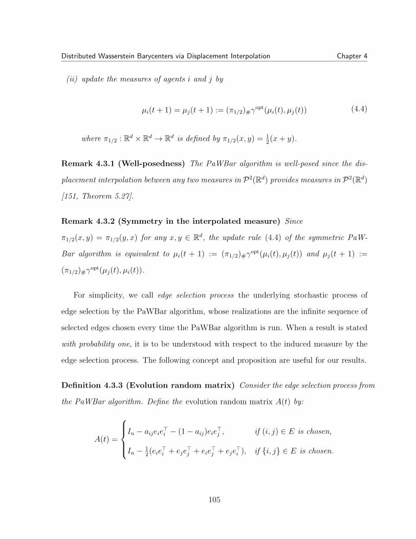
Distributed Wasserstein Barycenters via Displacement Interpolation Chapter 4
(ii) update the measures of agents i and j by
µi(t+ 1) = µj(t+ 1) := (π1/2)#γopt(µi(t), µj(t)) (4.4)
where π1/2 : Rd × Rd → Rd is defined by π1/2(x, y) = 12(x+ y).
Remark 4.3.1 (Well-posedness) The PaWBar algorithm is well-posed since the dis-
placement interpolation between any two measures in P2(Rd) provides measures in P2(Rd)
[151, Theorem 5.27].
Remark 4.3.2 (Symmetry in the interpolated measure) Since
π1/2(x, y) = π1/2(y, x) for any x, y ∈ Rd, the update rule (4.4) of the symmetric PaW-
Bar algorithm is equivalent to µi(t + 1) := (π1/2)#γopt(µi(t), µj(t)) and µj(t + 1) :=
(π1/2)#γopt(µj(t), µi(t)).
For simplicity, we call edge selection process the underlying stochastic process of
edge selection by the PaWBar algorithm, whose realizations are the infinite sequence of
selected edges chosen every time the PaWBar algorithm is run. When a result is stated
with probability one, it is to be understood with respect to the induced measure by the
edge selection process. The following concept and proposition are useful for our results.
Definition 4.3.3 (Evolution random matrix) Consider the edge selection process from
the PaWBar algorithm. Define the evolution random matrix A(t) by:
A(t) =
In − aijeie>i − (1− aij)eie>j , if (i, j) ∈ E is chosen,
In − 12(eie
>i + eje
>j + eie
>j + eje
>i ), if i, j ∈ E is chosen.
105

Distributed Wasserstein Barycenters via Displacement Interpolation Chapter 4
Proposition 4.3.3 (Convergence of products of evolution random matrices) Consider
the PaWBar algorithm. For the directed case with a strongly connected digraph:
limt→∞
t∏
τ=0
A(τ) = 1nλ>
for some random convex vector λ with probability one. For the symmetric case with a
connected undirected graph,
limt→∞
t∏
τ=0
A(τ) =1
n1n1
>n
with probability one.
Proof: We first prove the directed case. Observe that: (i) the sequence of random
matrices (A(t))t is i.i.d due to the edge selection process, (ii) A(t) has strictly positive
diagonal entries and is row-stochastic for any time t with probability one, (iii) E[A(t)],
the expected value of the evolution random matrix, corresponds to the adjacency matrix
of a strongly connected weighted digraph. Then, from these conditions (i)-(iii), we can
apply [33, Theorem 13.1] and obtain the sought convergence. The proof for the symmetric
case follows from applying [33, Corollary 13.2] instead.
4.3.2 Analysis of discrete measures
Theorem 4.3.4 (Wasserstein barycenters for discrete measures) Consider initial
measures µi,0i∈V , such that µi,0 = 1N
∑Nj=1 δxij , with xi1, . . . , x
iN ∈ Rd being distinct
points; i.e., µi,0 is a discrete uniform measure.
(i) Consider the directed PaWBar algorithm with an underlying strongly connected
digraph G; then, with probability one, for any i ∈ V ,
W2(µi(t), µ∞)→ 0 as t→∞, (4.5)
106

Distributed Wasserstein Barycenters via Displacement Interpolation Chapter 4
where the discrete uniform measure µ∞ solves the barycenter problem
µ∞ ∈ arg minν∈P2(Rd)
n∑
i=1
λiW2(ν, µi(T ))2
with λ = (λ1, . . . , λn)> being a random convex vector satisfying∏∞
τ=1A(τ) = 1nλ>
with probability one, and T ≥ 0 being some finite random time. If
maxi,j∈V W2(µi,0, µj,0) is sufficiently small, then T = 0 with probability one.
(ii) Consider the symmetric PaWBar algorithm with an underlying connected undi-
rected graph G; then, with probability one, for any i ∈ V ,
W2(µi(t), µ∞)→ 0 as t→∞, (4.6)
where the discrete uniform measure µ∞ solves the barycenter problem
µ∞ ∈ arg minν∈P2(Rd)
n∑
i=1
W2(ν, µi(T ))2 (4.7)
with T ≥ 0 being some finite random time. If maxi,j∈V W2(µi,0, µj,0) is sufficiently
small, then T = 0 with probability one.
Corollary 4.3.5 (Wasserstein barycenters for discrete measures on R) Consider
initial measures µi,0i∈V , such that µi,0 = 1N
∑Nj=1 δxij , with xi1, . . . , x
iN ∈ R such that
xi1 < · · · < xiN . Then, the directed, respectively symmetric, PaWBar algorithm computes
a randomized, respectively standard, Wasserstein barycenter of the initial measures.
Remark 4.3.6 (Discussion of our results) (i) The setting of Theorems 4.3.4 and
Corollary 4.3.5 has found applications in computational geometry, computer graph-
ics and digital image processing; e.g., see [146, 51, 30].
107
Distributed Wasserstein Barycenters via Displacement Interpolation Chapter 4
(ii) In Theorem 4.3.4, if all initial measures are sufficiently close in the Wasserstein
space, then the PaWBar algorithm computes one of their Wasserstein barycen-
ters. This sufficient condition is not a problem in practical applications where the
barycenter is used as an interpolation among measures that are known to be simi-
lar (e.g., measurements of the same object under noise). Moreover, Corollary 4.3.5
tells us that the initial measures in P(R) could be arbitrarily distant from each other
and still the PaWBar algorithm will compute one of their barycenters.
4.3.3 Analysis of absolutely continuous measures
We consider measures that are absolutely continuous with respect to the Lebesgue
measure. For any such measures µ, ν ∈ P2(Rd), there exists a unique optimal transport
map from µ to ν, which we denote by T νµ ; and we also denote T µµ = Id. It is also known
that there exists a unique Wasserstein barycenter when all the interpolated measures are
absolutely continuous with respect to the Lebesgue measure [6].
We focus on the class of measures that form a compatible collection. According
to [137, Definition 2.3.1], a collection of absolutely continuous measures C ⊂ P2(Rd) is
compatible if for all ν, µ, γ ∈ C, we have (T µγ T γν )#ν = (T µν )#ν.
Theorem 4.3.7 (Wasserstein barycenters for continuous measures in P2(Rd))
Consider initial measures µi,0i∈V that are absolutely continuous with respect to the
Lebesgue measure and that form a compatible collection. Let γ ∈ µi,0i∈V .
(i) Consider the directed PaWBar algorithm with an underlying strongly connected
digraph G; then, with probability one, for any i ∈ V ,
W2(µi(t), µ∞)→ 0 as t→∞,
108

Distributed Wasserstein Barycenters via Displacement Interpolation Chapter 4
where the absolutely continuous measure µ∞ =(∑n
j=1 λjTµj,0γ
)#γ is the barycenter
µ∞ = arg minν∈P2(Rd)
n∑
i=1
λiW2(ν, µi,0)2 (4.8)
with λ = (λ1, . . . , λn)> being a random convex vector satisfying∏∞
τ=1A(τ) = 1nλ>
with probability one.
(ii) Consider the symmetric PaWBar algorithm with an underlying connected undi-
rected graph G; then, with probability one, for any i ∈ V ,
W2(µi(t), µ∞)→ 0 as t→∞,
where the absolutely continuous measure µ∞ =(
1n
∑nj=1 T
µj,0γ
)#γ is the barycenter
µ∞ = arg minν∈P2(Rd)
n∑
i=1
W2(ν, µi,0)2.
The following corollary considers examples of measures relevant to our previous the-
orem. We use the term distribution and measure interchangeably for well-known proba-
bility measures with continuous distributions.
Corollary 4.3.8 (Examples of Wasserstein barycenters) Consider that initially ei-
ther
(i) all agents have a probability measure in P2(R) with continuous distribution; or
(ii) one agent has the standard Gaussian distribution on P2(Rd) and any other agent
i ∈ V has a Gaussian distribution µi,0 = N (mi,0,Σi,0) with mi,0 ∈ Rd and Σi,0 ∈
Rd×d being a positive definite matrix with the joint commutative property Σi,0Σj,0 =
Σj,0Σi,0 for any j ∈ V .
109

Distributed Wasserstein Barycenters via Displacement Interpolation Chapter 4
Consider the directed PaWBar algorithm with an underlying strongly connected digraph
G. Then, with probability one, W2(µi(t), µ∞)→ 0 as t→∞ for any i ∈ V , where µ∞ is
the Wasserstein barycenter of the initial measures. In particular,
• for case (i), µ∞ =(∑n
j=1 λjF−1µj,0 Fµi,0
)#µi,0 =
(∑nj=1 λjF
−1µj,0
)#L, with L being
the Lebesgue measure on [0, 1]; and
• for case (ii), µ∞ = N (m∞,Σ∞) with m∞ =∑n
j=1 λjmj,0 and Σ∞ ∈ Rd×d being a
positive definite matrix that satisfies Σ∞ =∑n
j=1 λj(Σ1/2∞ Σj,0Σ
1/2∞ )1/2;
with λ = (λ1, . . . , λn)> being a random convex vector such that∏∞
τ=1A(τ) = 1nλ> with
probability one.
Moreover, all the previous results also hold for the symmetric PaWBar algorithm
when G is a connected undirected graph, with the difference that the barycenters are now
the standard one, i.e., with λ = ( 1n, . . . , 1
n)> in the previous bullet points.
The work [8] proposes a non-distributed iterative algorithm tailored to compute the
Wasserstein barycenter of Gaussian distributions. However, to the best of our knowledge,
the PaWBar algorithm is the first algorithm that proposes a distributed computation
of randomized and standard Gaussian barycenters with closed-form iteration steps, as
indicated in the following proposition.
We remark that the distance interpolation between two Gaussian distributions is a
curve of Gaussian distributions.
Proposition 4.3.9 (PaWBar algorithm for Gaussian distributions) Assume any
agent i ∈ V has an initial distribution µi,0 = N (mi,0,Σi,0) with mi,0 ∈ Rd and Σi,0 ∈ Rd×d
being a positive definite matrix. At any time t, let mi(t) and Σi(t) be the mean and co-
variance matrix associated to agent i ∈ V .
110

Distributed Wasserstein Barycenters via Displacement Interpolation Chapter 4
(i) For the directed PaWBar algorithm, if (i, j) ∈ E is selected at time t, update the
Gaussian distribution of agent i according to:
mi(t+ 1) := (1− aij)mi(t) + aijmj(t),
Σi(t+ 1) := (1− aij)2Σi(t) + a2ijΣj(t)
+ aij(1− aij)(
(Σi(t)Σj(t))12 + (Σj(t)Σi(t))
12
).
(4.9)
(ii) For the symmetric PaWBar algorithm, if i, j ∈ E is selected at time t, update
the Gaussian distributions of agents i and j according to:
mi(t+ 1) := mj(t+ 1) =1
2(mi(t) +mj(t)),
Σi(t+ 1) := Σj(t+ 1) =1
4
(Σi(t) + Σj(t) + (Σi(t)Σj(t))
12 + (Σj(t)Σi(t))
12
).
(4.10)
Then, the results stated in Corollary 4.3.8, under the conditions indicated therein, hold.
Proof: For statement (i), equation (4.9) results from the displacement interpolation
between Gaussian distributions, as seen in [41], and thus implements equation (4.3).
Case (ii) follows similarly.
Remark 4.3.10 (Examples of measures for Theorem 4.3.7) We refer to [137, Sec-
tion 2.3] and [27] for more examples of measures that form compatible collections and
their statistical applications.
Remark 4.3.11 (Further propertiesof the randomized Wasserstein barycenter)
The results in [161] can be applied to characterize the mean and covariance matrix asso-
ciated to the random convex vector present in the randomized Wasserstein barycenter in
Theorem 4.3.4, Corollary 4.3.5, Theorem 4.3.7, and Corollary 4.3.8. This characteriza-
tion numerically depends on the values of the time-invariant probabilities associated with
the edge selection process.
111

Distributed Wasserstein Barycenters via Displacement Interpolation Chapter 4
We propose the following conjecture.
Conjecture 2 (Computation under more general continuous measures) The
convergence results of the PaWBar algorithm in Theorem 4.3.7 also hold for general
absolutely continuous measures, i.e., ones which do not necessarily form a compatible
collection.
We provide some numerical evidence that Conjecture 2 is true at least for the case
where all agents initially have multivariate Gaussian distributions that do not form a
compatible collection. In the numerical evidence presented in Figure 4.1 and Figure 4.2,
we use the updates presented in Proposition 4.3.9, and we only focus on the evolution of
the agents’ covariance matrices (the mean values evolve linearly and are easy to verify
they converge to the mean of the Wasserstein barycenter). In this Gaussian setting, we
also performed similar simulations to the ones in both figures but using the symmetric
PaWBar algorithm with connected graphs; and we obtained convergence to the standard
Wasserstein barycenter.
4.3.4 Analysis of general measures
So far, we presented convergence results to a Wasserstein barycenter for classes of
discrete (Theorem 4.3.4 and Corollary 4.3.5) and absolutely continuous (Theorem 4.3.7
and Corollary 4.3.8) measures. In these cases an optimal transport map exists between
any two agents’ measures at every time. Now we analyze the PaWBar algorithm on
general measures in P2(Rd). Examples of this setting include cases where there may not
exist an optimal transport map between two or more initial measures, or cases where there
could exist a mix of discrete and absolutely continuous initial measures. We prove that
agents converge to consensus with probability one in more restricted graph topologies,
112

Distributed Wasserstein Barycenters via Displacement Interpolation Chapter 4
1
2 3
45 0 10 20 30 40 50 60 70 80
iterations
0
0.2
0.4
0.6
0.8
1
1.2
erro
r
Agent 1Agent 2Agent 3Agent 4Agent 5
Figure 4.1: Consider five agents that initially have multivariate Gaussian distributionson R5, with their covariance matrices being randomly generated. On the left, wepresent the underlying digraph over which the PaWBar algorithm is run. The weightassociated to all edges is 0.75. We first fix a realization of the edge selection processby fixing the seed of the random number generator in our scientific software. Then,we compute the covariance matrix Σ∞ of the Wasserstein barycenter that would beobtained with the weights corresponding to the entries of any row of the product ofevolution random matrices after a long period of time. The numerical computationof Σ∞ follows the scheme proposed in [8]. On the right, each of the five plottedcurves corresponds to the evolution of the error quantity ‖Σi(t)− Σ∞‖F for each agenti ∈ 1, . . . , 5, where Σi(t) is the value of agent i’s covariance matrix at iteration t,and ‖·‖F is the Frobenius norm. All agents asymptotically reach consensus and theircovariance matrices become the covariance matrix of the randomized Wassersteinbarycenter, thus giving evidence for the veracity of Conjecture 2 at least for theGaussian case.
and that the consensus measure satisfies a necessary condition known to characterize
barycenters for certain classes of measures.
Theorem 4.3.12 (Consensus result for general measures) Consider the PaWBar
algorithm with an underlying graph G which is either
(i) a cycle graph for the directed case, or
(ii) a line graph for the symmetric case;
and with the agents having initial measures µi,0 ∈ P2(Rd), i ∈ V . Then, with probability
113

Distributed Wasserstein Barycenters via Displacement Interpolation Chapter 4
1
2 3
45 0 10 20 30 40 50 60 70 80
iterations
0
0.2
0.4
0.6
0.8
1
1.2
erro
r
Agent 1Agent 2Agent 3Agent 4Agent 5
Figure 4.2: Consider five agents that initially have multivariate Gaussian distributionson R5, with their covariance matrices being randomly generated. The setting andmethodology for computing the plot on the right is similar to the one described inFigure 4.1, with the difference that now the underlying digraph is a cycle (as seenon the left). All agents asymptotically reach consensus and their covariance matricesbecome the covariance matrix of the randomized Wasserstein barycenter.
one, for any i ∈ V ,
W2(µi(t), µ∞)→ 0 as t→∞, (4.11)
where µ∞ ∈ P2(Rd) is a random measure whose possible values depend on the realization
of the edge selection process. If µi,0 = µj,0 for any i, j ∈ V , then µ∞ = µi,0 with probability
one.
Moreover, for either the directed or symmetric case, and with probability one,
supp(µ∞) ⊆ cl
n∑
i=1
λixi
∣∣∣∣ xi ∈ supp(µi,0), λi ≥ 0, i ∈ V, andn∑
i=1
λi = 1
, (4.12)
with cl indicating the closure operation for sets.
Remark 4.3.13 (Theorem 4.3.12 and Wasserstein barycenters) Equation (4.12)
is known to be satisfied when µ∞ is a Wasserstein barycenter of measures that are ab-
solutely continuous with respect to the Lebesgue measure, or discrete with finite sup-
port [6, 13]. However, the characterization of the consensus value in our theorem does
114

Distributed Wasserstein Barycenters via Displacement Interpolation Chapter 4
not state any sufficient condition under which the converged consensus random measure
is a Wasserstein barycenter or not: this is an open problem for further research.
4.4 Proofs of results in Section 4.3
4.4.1 Proofs of results in Subsection 4.3.2
Proof: [Proof of Theorem 4.3.4] Since measures µi,0 and µj,0, i, j ∈ V , are discrete
uniform, we have W 22 (µi,0, µj,0) = minσ∈ΣN
1N
∑Nk=0
∥∥∥xik − xjσ(k)
∥∥∥2
2[169, 146], with ΣN
being the set of all possible permutations of the elements in 1, . . . , N; i.e., any per-
mutation map σ ∈ ΣN is a bijective function σ : 1, . . . , N → 1, . . . , N. Then,
the displacement interpolation between any of the initial measures provides discrete
measures. Now, consider σ ∈ ΣN from solving the optimal transport problem from
µi,0 to µj,0, i.e., γopt(µi,0, µj,0) = 1N
∑Nk=0 δ(xik,x
jσ(k)
). Consider two arbitrary points (xik1,
xjσ(k1)), (xik2, xjσ(k2)) ∈ supp(γopt(µi,0, µj,0)). Then, for any aij ∈ (0, 1), the displacement
interpolation implies the existence of some zk1(aij), zk2(aij) ∈ supp((πaij)#µi,0), such that
zk1(aij) = (1−aij)xik1+aijx
jσ(k1) and zk2(aij) = (1−aij)xik2
+aijxjσ(k2). Now, since the op-
timal transport plan γopt(µi,0, µj,0) has cyclically monotone support [169, Section 2.3], we
can follow the treatment in [170, Chapter 8] and conclude that there exists no aij ∈ (0, 1)
such that zk1(aij) = zk2(aij). As a consequence, supp((πaij)#µi,0) has N (different) ele-
ments for any possible edge weight aij, i.e., (πaij)#µi,0 is a discrete uniform measure. It
is easy to show by induction that in either the directed or symmetric PaWBar algorithm,
µi(t) is a discrete uniform distribution for any i ∈ V and time t with probability one.
We now introduce some notation. Given A ∈ Rm×m, let diagi,k(A) ∈ Rkm×km be the
k × k block-diagonal matrix such that its ith block has the matrix A and the rest of
blocks are Im. Given A,B ∈ Rm×m, let diagij,k(A,B) ∈ Rkm×km be the k × k block-
115
Distributed Wasserstein Barycenters via Displacement Interpolation Chapter 4
diagonal matrix such that its ith and jth blocks are the matrices A and B respectively,
and the rest of blocks are Im. Let xi(t) ∈ RNd be a vector stacking the elements of
supp(µi(t)), which we call the support vector. Note that since the measures are discrete
uniform at every time t (with probability one), the order of the elements xik(t) ∈ Rd,
k ∈ 1, . . . , N, in the vector xi(t) can be arbitrary; but for convenience we denote it as
xi(t) = (xi1(t), · · · , xiN(t))>. For any i, j ∈ V and time t, let σij,t ∈ ΣN be an optimal
transport map from µi(t) to µj(t); and let σii,t(k) = k and σji,t = σ−1ij,t.
We now focus on proving statement (i). Assume (i, j) ∈ E is selected at time t. Then,
xik(t+ 1) = (1− aij)xik(t) + aijxjσij,t(k)(t), k ∈ 1, . . . , N, i.e.,
xi(t+ 1) = (1− aij)xi(t) + aij(P (t)⊗ Id)xj(t) (4.13)
with the permutation matrix P (t) ⊗ Id defined by the permutation matrix P (t) ∈
0, 1N×N whose kth row is e>σij,t(k). Indeed, with Qij,t = P (t)⊗ Id,
W 22 (µi(t), µj(t)) =
1
N
∥∥xi(t)−Qij,txj(t)∥∥2
2.
We make the following claim:
(i.a) for any i∗, j∗ ∈ V , i∗ 6= j∗, ε > 0 and time t, the event “W2(µi∗(t+T ), µj∗(t+T )) < ε
for some finite T > 0” has positive probability.
We prove the claim. Define d(i, j, σi, σj, ti, tj) :=(∑N
k=11N
∥∥xiσi(k)(ti) − xjσj(k)
(tj)∥∥2
2
) 12,
for i, j ∈ V , σi, σj ∈ ΣN . Consider any i∗, j∗ ∈ V and ε > 0. Since G is strongly
connected, there exists a shortest directed path Pi∗→j∗ from i∗ to j∗ of some length L.
Let Pi∗→j∗ = ((i∗, `1), . . . , (`L−1, j∗)). Now, pick positive numbers ε1, . . . , εL such that
∑Li=1 εi < ε. Consider any time t. Then, we can first select T1 times the edge (`L−1, j
∗)
116

Distributed Wasserstein Barycenters via Displacement Interpolation Chapter 4
so that
d(`L−1, j∗, σ−1
`L−1j∗,t+T1, Id, t+ T1, t) = (1− a`L−1j∗)
T1d(`L−1, j∗, σ−1
`L−1j∗,t, Id, t, t) < εL.
Then, we can select T2 times the edge (`L−2, `L−1) so that
d(`L−2, `L−1, σ−1`L−2`L−1,t+T1+T2
σ−1`L−1j∗,t+T1
, σ−1`L−1j∗,t+T1
, t+ T1 + T2, t+ T1) < εL−1,
and we can continue like this until finally selecting TL times the edge (i∗, `1) such that
d(i∗, `1, σ, σ−1
`1`2,t+∑L−1i=0 Ti
· · · σ−1`L−1j∗,t
, t+ T, t+∑L−1
i=1 Ti) < ε1 with σ = σ−1i∗`1,t+T
· · ·
σ−1`L−1j∗,t
and T =∑L
i=1 Ti. Then,
W2(µi∗(t+ T ), µj∗(t+ T )) ≤ (N∑
k=1
1
N
∥∥∥xi∗σ(k)(t+ T )− xj∗k (t+ T )∥∥∥
2
2)
12 <
L∑
i=1
εi < ε.
where the first inequality follows by definition of the Wasserstein distance, and the second
inequality from both the triangle inequality and the fact that xj∗
k (t+T ) = xj∗
k (t), x`L−1
k (t+
T ) = x`L−1
k (t+T1), . . . , x`1k (t+T ) = x`1k (t+∑L−1
i=1 Ti). Moreover, our construction implies
W2(µp(t+ T ), µj∗(t+ T )) < ε for any p ∈ Pi∗→j∗ . (4.14)
Now, consider any m ∈ V and construct a directed acyclic subgraph G′ = (V,E ′),
E ′ ⊂ E, of G as follows: m is the unique node with zero out-degree (i.e, (m, i) /∈ E ′
for any i ∈ V ) and there exists a unique directed path from any node i ∈ V \ m to
m. Such subgraph G′ exists because G is strongly connected. Consider any ε > 0 and
time t. Then, the selection process just described above can make all nodes m with
zero in-degree in G′ (i.e., any m ∈ V such that (i, m) /∈ E ′ for any i ∈ V \ m) satisfy
W2(µm(t+T ), µm(t+T )) = W2(µm(t+T ), µm(t)) < ε2
for some T . Then, as a consequence
117

Distributed Wasserstein Barycenters via Displacement Interpolation Chapter 4
of (4.14), W2(µi(t + T ), µj(t + T )) < ε2
for any i ∈ V , and the triangle inequality then
implies W2(µi(t + T ), µj(t + T )) < ε for any j ∈ V . Finally, for any i, j ∈ V , the event
“W2(µi(t + T ), µj(t + T )) < ε for some T > 0” has a positive probability to occur at
any time t because any selection of a finite sequence of edges has positive probability to
occur at any time t. This finishes the proof of claim (i.a).
Now, note that the event in result (i.a), due to its persistence, will eventually happen
with probability one. Assume it happens at time t. Then, we claim that ε in this event
could have been chosen so that, for any time t′ ≥ t and any i, j, p ∈ V ,
(i.b) σij,t′ = σij,t, and
(i.c) σij,t′ = σip,t′ σpj,t′ .
Now we prove the claim. Firstly, note that from (i.a) and the fact that the measures are
discrete uniform at every time with probability one, we can consider a small enough ε
such that for any i, j ∈ V and any permutation map σ 6= σij,t,
W2(µi(t), µj(t)) =( 1
N
N∑
k=1
∥∥∥xik(t)− xjσij,t(k)(t)∥∥∥
2
2
) 12< ε and
2ε <( 1
N
N∑
k=1
∥∥∥xik(t)− xjσ(k)(t)∥∥∥
2
2
) 12.
(4.15)
Such choice of ε implies that σip,tσpj,t = σij,t for any i, j, p ∈ V ; otherwise, if σip,tσpj,t 6=
σij,t, then we obtain a contradiction:
2ε <( 1
N
N∑
k=1
∥∥∥xik(t)− xjσip,tσpj,t(k)(t)∥∥∥
2
2
) 12
=( 1
N
N∑
k=1
∥∥∥xiσpi,t(k)(t)− xjσpj,t(k)(t)∥∥∥
2
2
) 12
≤( 1
N
N∑
k=1
∥∥∥xiσpi,t(k)(t)− xpk(t)∥∥∥
2
2
) 12
+( 1
N
N∑
k=1
∥∥∥xpk(t)− xjσpj,t(k)(t)∥∥∥
2
2
) 12< 2ε.
We just proved that (i.c) holds for t′ = t. Note that (i.b) for t′ = t is trivial. Now,
118

Distributed Wasserstein Barycenters via Displacement Interpolation Chapter 4
assume any (i∗, j∗) ∈ E is selected at time t. Then, for any j ∈ V \ i∗, j∗, using the
identity Qj∗j,t = Qj∗i∗,tQi∗j,t from (i.c) for t′ = t implies
∥∥xi∗(t+ 1)−Qi∗j,txj(t+ 1)
∥∥2
(4.16)
≤ (1− ai∗j∗)∥∥xi∗(t)−Qi∗j,tx
j(t)∥∥
2+ ai∗j∗
∥∥Qi∗j∗,txj∗(t)−Qi∗j,tx
j(t)∥∥
2
= (1− ai∗j∗)∥∥xi∗(t)−Qi∗j,tx
j(t)∥∥
2+ ai∗j∗
∥∥xj∗(t)−Qj∗j,txj(t)∥∥
2
< (1− ai∗j∗)ε√N + ai∗j∗ε
√N = ε
√N ;
likewise, we immediately obtain 1√N‖xi(t+ 1)−Qij,tx
j(t+ 1)‖2 < ε for any i ∈ V \
i∗, j, and 1√N
∥∥xi∗(t+ 1)−Qi∗j∗,txj∗(t+ 1)
∥∥2< (1− ai∗j∗)ε < ε. In summary,
1√N‖xi(t+ 1)−Qij,tx
j(t+ 1)‖2 < ε for any i, j ∈ V , which implies σij,t+1 = σij,t for any
i, j ∈ V ; i.e., (i.b) holds for t′ = t + 1. Now, to prove claim (i.c) holds for t′ = t + 1, we
must first prove that (4.15) holds for time t+ 1.
Set y1(t) := x1(t),y2(t) = Q12,tx2(t), . . . ,yn(t) = Q1n,tx
n(t) (this labeling is arbi-
trary and any other i ∈ V \ 1 could have been chosen to define Qi1, . . . , Qin) and
yi(t) = (yi1(t), . . . , yiN(t))>, yi1(t) ∈ Rd, i ∈ 1, . . . , n. For any k ∈ 1, . . . , N, let Lk(t)
be the convex hull of the set y1k(t), . . . , y
nk (t). For any p, q ∈ 1, . . . , N, define the
distance between Lp(t) and Lq(t) as dpq(t) = infw1∈Lp(t),w2∈Lq(t) ‖w1 − w2‖2. Assuming
that (i∗, j∗) ∈ E is selected at time t, our result (i.b) for t′ = t + 1 and (4.13) imply
that yi∗
k (t + 1) = (1 − ai∗j∗)yi∗
k (t) + ai∗j∗yj∗
k ∈ Lk(t), k ∈ 1, . . . , N. Obviously, for
any j ∈ V \ i∗, yjk(t + 1) = yjk(t) ∈ Lk(t), k ∈ 1, . . . , N. Then, Li(t + 1) ⊆ Li(t)
for any i ∈ 1, . . . , N, and thus dpq(t) ≤ dpq(t + 1) for any p, q ∈ 1, . . . , N. Now,
for any i, j ∈ V , time τ ≥ t, and permutation map σ 6= Id, we have dkσ(k)(τ) ≤∥∥∥yik(τ)− yjσ(k)(τ)
∥∥∥2
=⇒ (∑N
k=1 d2kσ(k)(τ))
12 ≤ (
∑Nk=1
∥∥∥yik(τ)− yjσ(k)(τ)∥∥∥
2
2)
12 . Now, we need
to consider two cases. In the first case we consider
119

Distributed Wasserstein Barycenters via Displacement Interpolation Chapter 4
2ε < minσ∈ΣN ,σ 6=Id(1N
∑Nk=1 d
2kσ(k)(t))
12 . Then,
2ε < (1
N
N∑
k=1
d2kσ(k)(t+ 1))
12 ≤ (
1
N
N∑
k=1
∥∥∥yik(t+ 1)− yjσ(k)(t+ 1)∥∥∥
2
2)
12
for any permutation map σ 6= Id; and (i.b) for t′ = t + 1 and (i.c) for t′ = t imply
2ε < ( 1N
∑Nk=1
∥∥∥xik(t+ 1)− xjσ′(k)(t+ 1)∥∥∥
2
2)
12 with σ′ = σi1,t+1 σ σ1j,t+1 6= σij,t+1.
Thus, (4.15) holds for time t + 1 in this first case. Now, we consider the second
case 2ε ≥ minσ∈ΣN ,σ 6=Id(1N
∑Nk=1 d
2kσ(k)(t))
12 . Then, due to G being strongly connected
and dpq(τ)τ≥t being a nondecreasing sequence for any p, q ∈ 1, . . . , N, we can fol-
low the proof of result (i.a) and arbitrarily reduce the diameter of the set Lk for any
k ∈ 1, . . . , N at some future time t, i.e., L(t) ⊂ L(t). This diameter reduction can
be chosen such that dij(t) > dij(t) for any i, j ∈ 1, . . . , N, and this increase on the
distances between sets can be done so that 2ε′ < minσ∈ΣN ,σ 6=Id(1N
∑Nk=1 d
2kσ(k)(t))
12 for
some 0 < ε′ < ε. In other words, we are in the first case at time t. After this change,
we will never be in the second case again for any time after t with probability one. In
summary, we just proved the conditions in equation (4.15) can be made to hold for time
t+ 1, and so (i.c) holds for t′ = t+ 1.
Now, assume results (i.b) and (i.c) hold for time t′ = τ ≥ t, and (4.15) holds for time
τ . Following the proof just presented above, we easily establish that (i.b) and (i.c) hold
for t′ = τ + 1 and that (4.15) holds for time τ + 1. Then, by induction, we proved our
initial claim about (i.b) and (i.c).
Now, set x(t) = (x1(t), . . . ,xn(t))> ∈ RnNd. Assume (i, j) ∈ E is selected at any time
t ≥ 0. Then, (4.13) becomes
x(t+ 1) = B(t)x(t) (4.17)
with the row-stochastic matrix B(t) = diagj,n(P (t)> ⊗ Id)(A(t)⊗ INd) diagj,n(P (t)⊗ Id)
120

Distributed Wasserstein Barycenters via Displacement Interpolation Chapter 4
(recall the permutation matrix P (t) was defined after (4.13)).
Consider an initial vector x(0) and a fixed realization of the edge selection process.
Now consider x′(0) = diag(P1⊗ Id, . . . , Pn⊗ Id)x(0) with arbitrary permutation matrices
P1, . . . , Pn ∈ 0, 1N×N . Notice that both x(0) and x′(0) represent the supports of the
same group of measures µi,0i∈V but may be the case that x(0) 6= x′(0). We claim that
x′(t) = diag(P1 ⊗ Id, . . . , Pn ⊗ Id)x(t) for any time t. (4.18)
To prove this claim, first recall that we have a fixed realization of the edge selection
process. Assume (i, j) ∈ E is selected at time t = 0 and obtain x(1) = B(0)x(0).
Likewise, x′(1) = B′(0)x′(0), with B′(0) = diagj,n(P ′(0)>⊗Id)(A(0)⊗INd) diagj,n(P ′(0)⊗
Id), is the update that results if the algorithm starts with initial vector x′(0). Then,
P ′(0)⊗ Id = (Pi ⊗ Id)(P (0)⊗ Id)(P>j ⊗ Id) = (PiP (0)P>j )⊗ Id.
After some algebraic work, we obtainB′(0) = diagij,n(Pi, Pj)B(0) diagij,n(P>i , P>j ). Then,
x′(1) = diagij,n(Pi, Pj)B(0) diagij,n(P>i , P>j )x′(0)
= diagij,n(Pi, Pj)B(0) diagij,n(P>i , P>j ) diag(P1, . . . , Pn)x(0)
= diag(P1, . . . , Pn)B(0)x(0) = diag(P1, . . . , Pn)x(1).
Finally (4.18) is easily proved by induction, and the claim is proved.
Now, from results (i.a), (i.b) and (i.c), there exists some random time T > 0 such
that, with probability one: for any time t ≥ T and any i, j, p ∈ V , σij,t = σij,T and
σij,t = σip,t σpj,t. Consider such time T , which is now a deterministic function of x(0)
since we have a fixed realization of the edge selection process. Without loss of generality,
121

Distributed Wasserstein Barycenters via Displacement Interpolation Chapter 4
as a consequence of (4.18), we can assume we started the algorithm with the initial
support vectors Q1i,Txi(0)i∈V at time t = 0. Then, it is easy to prove that B(t) =
A(t) ⊗ INd for any t ≥ T , i.e., B(t) has an associated permutation matrix P (t) = IN .
Then, Proposition 4.3.3 let us conclude that limt→∞∏t
τ=T B(τ) = (1nλ>)⊗ INd for some
convex vector λ. Thus, xi(∞) =∑n
j=1 λjxj(T ), i ∈ V .
It remains to prove that µ∞ corresponds to a Wasserstein barycenter. Let us for-
mulate the Wasserstein barycenter problem minν∈P2(Rd)
∑ni=1 λiW2(ν, µi(T ))2. Since the
measures µi(T )i∈V have finite support, any barycenter is a discrete measure with finite
support [13]. Moreover, since all the measures are uniform, we can consider a minimizer
with a discrete uniform distribution. We now prove that µ∞ is such a minimizer. Firstly,
by construction and the fact that (4.15) holds for t ≥ T , we have
W2(µ∞, µi(T ))2 =1
N
N∑
j=1
∥∥∥∥∥n∑
k=1
λkxkj (T )− xij(T )
∥∥∥∥∥
2
2
< 2ε <1
N
N∑
j=1
∥∥∥∥∥n∑
k=1
λkxkσk(j)(T )− xiσi(j)(T )
∥∥∥∥∥
2
2
for any σi ∈ ΣN , σi 6= Id, i ∈ V . Then,
n∑
i=1
λiW2(µ∞, µi(T ))2 <1
N
n∑
i=1
λi
N∑
j=1
∥∥∥∥∥n∑
k=1
λkxkσk(j)(T )− xiσi(j)(T )
∥∥∥∥∥
2
2
≤ 1
N
n∑
i=1
λi
N∑
j=1
∥∥∥yi − xiσi(j)(T )∥∥∥
2
2
for any y = (y1, . . . , yn)> ∈ RNd. The last inequality of the previous expression is
proved by using first optimality conditions to minimize the differentiable and strictly
convex functional of y (i.e., set the gradient with respect to y equal to the zero vec-
tor). Now, take yi 6= yj ∈ Rd for any i, j ∈ 1, . . . , N, define the discrete uniform
122

Distributed Wasserstein Barycenters via Displacement Interpolation Chapter 4
measure ν = 1N
∑Nj=1 δyj , yj ∈ Rd; and let σi, i ∈ V , be such that W2(ν, µi(T ))2 =
1N
∑ni=1 λi
∑Nj=1
∥∥∥yi − xiσi(j)(T )∥∥∥
2
2. Then, our recent analysis implies that: (1) if there
exists i ∈ V such that σi 6= Id, then∑n
i=1 λiW2(µ∞, µi(T ))2 <∑n
i=1 λiW2(ν, µi(T ))2;
(2) if σi = Id for all i ∈ V , then∑n
i=1 λiW2(µ∞, µi(T ))2 ≤∑ni=1 λiW2(ν, µi(T ))2.
Given the generality of ν, cases (1) and (2) together imply that µ∞ is a Wasserstein
barycenter.
Finally, all of our previous results hold with probability one because we considered
an arbitrary realization of the edge selection process for our analysis (note that λ now
becomes a random convex vector). This concludes the proof of statement (i).
We now focus on proving statement (ii). Assume i, j ∈ E is selected at time t.
Without loss of generality, the update of the PaWBar algorithm can be set as xik(t+1) =
12xik(t) + 1
2xjσij,t(k)(t) and xjk(t+ 1) = 1
2xjk(t) + 1
2xiσji,t(k)(t), k ∈ 1, . . . , N; i.e.,
xi(t+ 1) =1
2xi(t) +
1
2(P (t)⊗ Id)xj(t),
xj(t+ 1) =1
2xj(t) +
1
2(P (t)> ⊗ Id)xi(t)
(4.19)
recalling that the permutation matrix P (t) ∈ 0, 1N×N has e>σij,t(k) as its kth row.
We make the following claim:
(ii.a) for any i∗, j∗ ∈ V , i∗ 6= j∗, ε > 0 and time t, the event “W2(µi∗(t+T ), µj∗(t+T )) < ε
for some finite T > 0” has positive probability.
Now, we prove the claim. Let us fix a spanning tree G′ of G. For any i, j ∈ V , let Pi−jdenote the unique path between i and j in G′. Let
U(t) = maxi,j∈V
∑
p,q∈Pi−j
W2(µp(t), µq(t)).
Let k, ` ∈ argU(t) and Pk−l = (k, p1, . . . , pL−1, `), i.e., edge k, p1 is followed by
123

Distributed Wasserstein Barycenters via Displacement Interpolation Chapter 4
p1, p2 and so on until pL−1, `. Case 1) W2(µk(t), µp1(t)) 6= 0. For simplicity we also
assume W2(µi(t), µj(t)) 6= 0 for any i, j ∈ Pk−`; otherwise, if there exists i∗, j∗ ∈ Pk−`such that W2(µi∗(t), µj∗(t)) = 0, we would need to use a similar analysis to Case 2) which
will be treated later. Select k, p1 at time t. If Pk−` contains only one element, then
p1 = ` and W2(µk(t + 1), µ`(t + 1)) = 0 < U(t) = W2(µk(t), µ`(t)). Now, consider Pk−`contains two or more elements. Set U(t) =
∑p,q∈Pk−`\k,p1,p1,p2W2(µp(t), µq(t))
(with p2 = ` and U(t) = 0 if Pk−` only has two elements). Then
∑
p,q∈Pk−`
W2(µp(t+ 1), µq(t+ 1)) = U(t) +1√N‖xp1(t+ 1)−Qp1p2,t+1x
p2(t)‖2
≤ U(t) +1√N‖xp1(t+ 1)−Qp1p2,tx
p2(t)‖2
≤ U(t) +1
2W2(µp1(t), µp2(t)) +
1
2√N
∥∥Qp1k,txk(t)−Qp1p2,tx
p2(t)∥∥
2
≤ U(t) +1
2W2(µp1(t), µp2(t)) +
1
2√N
∥∥Qp1k,txk(t)− xp1(t)
∥∥2
+1
2√N‖xp1(t)−Qp1p2,tx
p2(t)‖2
= U(t) +W2(µp1(t), µp2(t)) +1
2W2(µk(t), µp1(t)),
and so∑p,q∈Pk−`W2(µp(t + 1), µq(t + 1)) < U(t). Therefore, for any length of Pk−`,
if U(t + 1) ≤ ∑p,q∈Pk−`W2(µp(t + 1), µq(t + 1)), then U(t + 1) < U(t). If U(t + 1) >∑p,q∈Pk−`W2(µp(t+ 1), µq(t+ 1)), then we can choose k, ¯ ∈ argU(t+ 1) and, using
the analysis just presented, obtain∑p,q∈Pk−¯
W2(µp(t+ 2), µq(t+ 2)) < U(t+ 1). If this
does not imply U(t + 2) < U(t), we can keep iterating this procedure until, eventually,
obtain U(t+T ) < U(t) for some T > 0. Case 2) W2(µk(t), µp1(t)) = 0. In this case, we do
not select the edge k, p1, but we consecutively check the edges along Pk−` starting from
k, p1 and look for the first i∗, j∗ ∈ Pk−` such that W2(µi∗(t), µj∗(t)) 6= 0. We select
this edge and a similar analysis to Case 1) implies that∑p,q∈Pk→`W2(µp(t+ 1), µq(t+
124

Distributed Wasserstein Barycenters via Displacement Interpolation Chapter 4
1)) ≤ U(t). Then, we select the edge previous to i∗, j∗ and continue to successively
select the preceding edges until reaching the first edge k, p1. Once this edge is selected,
say at time t, the proof of case Case 1) let us conclude that∑p,q∈Pk−`W2(µp(t +
1), µq(t + 1)) < U(t), and we can continue the analysis of Case 1) until we have that
U(t+ T ) < U(t) ≤ U(t) for some T > 0. In conclusion, we proved the existence of some
finite sequence of selected edges such that U(t+T ) < U(t) for some T > 0. Moreover, we
can iterate selections of such sequences to arbitrarily reduce the value of U(t) after some
finite time. Finally, claim (ii.a) follows from the fact that maxi,j∈V W2(µi(t), µj(t)) ≤ U(t)
and that any finite sequence of edges has a positive probability of being consecutively
selected at any time t.
We can now follow the same analysis as in the proof of statement (i) of the theorem
(using result (ii.a) and its proof instead of (i.a)) to conclude that results (i.b) and (i.c)
also hold for the symmetric PaWBar algorithm.
Now, assume i, j ∈ E is selected at time t ≥ 0. Then, (4.19) becomes
x(t+ 1) = C(t)x(t), (4.20)
with the matrix C(t) = diagi,n(P (t)⊗ Id)(A(t)⊗ INd) diagi,n(P>(t)⊗ Id).
We fix a realization of the edge selection process. Consider any initial vector x(0) and
x(0)′ = diag(P1 ⊗ Id, . . . , Pn ⊗ Id)x(0) with arbitrary permutation matrices P1, . . . , Pn ∈
0, 1N×N . As in the proof of statement (i), it is possible to prove that x′(t) = diag(P1⊗
Id, . . . , Pn⊗ Id)x(t) for any t after some algebraic work. From here, we can closely follow
the proof of statement (i) to conclude the proof for statement (ii).
Proof: [Proof of Corollary 4.3.5] We follow the notation and proof of Theorem 4.3.4.
Note that the entries of xi(0) = (xi1, . . . , xiN)>, i ∈ V , are sorted in ascending order.
Then, W 22 (µi,0, µj,0) = 1
N
∑Nk=0(xik−xjk)2 for i, j ∈ V . Now, consider the directed PaWBar
125

Distributed Wasserstein Barycenters via Displacement Interpolation Chapter 4
algorithm and that (i, j) ∈ E is selected at time t = 0. Then xi(1) = (1 − aij)xi(0) +
aijxj(0) and xi(1) has its entries sorted in ascending order. Then, it is easy to prove
by induction that, at every time t, xi(t) for any i ∈ V is sorted in ascending order with
probability one. Considering x(t) = (xi(t), . . . ,xn(t))> ∈ RnN , we have that x(t + 1) =
(A(t)⊗ IN)x(t) and so x(t) = (∏t
i=0 A(i)⊗1N)x(0). Then, we conclude the proof for the
directed PaWBar algorithm by using Proposition 4.3.3 and the fact that∑n
i=1 λixi(0) ∈
arg min y∈Rdyi<···<yn
1N
∑ni=1 λi
∑Nk=0(yk − xik)2 for any convex vector λ ∈ Rn. The symmetric
case is proved similarly.
4.4.2 Proofs of results in Subsection 4.3.3
Proof: [Proof of Theorem 4.3.7] Consider the following notation: for any i, j, k ∈ V ,
denote (Tα3α2Tα2
α1)#α1 = (Tα3
α1)#α1 by Tα3
α2Tα2
α1= Tα3
α1for absolutely continuous measures
α1, α2, α3 ∈ P2(Rd).
First of all, it is known that a displacement interpolation between any of the absolutely
continuous initial measures results in a curve of absolutely continuous measures [151].
Then, with probability one, µi(t) is absolutely continuous for every i ∈ V and time
t. This also implies all measures up to any time form a compatible collection with
probability one. To see this, fix any γ ∈ µi,0i∈V and assume any (i, j) ∈ E is selected
at time zero. Clearly, µi(1) = (Tµi(1)γ )#γ = (T
µi(1)γ T γµi,0)#µi,0 and µi(1) = (T
µi(1)µi,0 )#µi,0,
thus (a) Tµi(1)µi,0 = T
µi(1)γ T γµi,0 and T
µi,0µi(1) = T
µi,0γ T γµi(1). To obtain the second equality
in (a), we used the identity (Tα1α2
)−1 = Tα2α1
that holds for two absolutely continuous
measures α1, α2 ∈ P2(Rd). Now, (Tµi(1)γ )#γ = (T
µi(1)µi,0 )#µi,0 = (T
µi(1)µi,0 )#(T
µi,0γ )#γ =
(Tµi(1)µi,0 T µi,0γ )#γ, and so (b) T
µi(1)γ = T
µi(1)µi,0 T µi,0γ and T γµi(1) = T γµi,0 T
µi,0µi(1). Now, we do a
push-forward operation under the map Tµi,0µi(1) on both sides of the first equality in (b) to
obtain (Tµi,0µi(1) T
µi(1)γ )#γ = (T
µi,0µi(1) T
µi(1)µi,0 T µi,0γ )#γ =⇒ (T
µi,0µi(1) T
µi(1)γ )#γ = (T
µi,0γ )#γ,
126

Distributed Wasserstein Barycenters via Displacement Interpolation Chapter 4
and so (c) Tµi,0γ = T
µi,0µi(1) T
µi(1)γ and T γµi,0 = T γµi(1) T
µi(1)µi,0 . Then, from results (a)-
(c) and the fact that the selected edge at time zero was arbitrary, we conclude that
µ1(1), . . . , µn(1) ∪ µ1(0), . . . , µn(0) forms a compatible collection with probability
one. Indeed, we can easily prove by induction that, with probability one, ∪tτ=0µi(τ)i∈Vis a compatible collection.
Now, assume any (i, j) ∈ E is selected at time zero. Then,
µi(1) = ((1− aij)Id+ aijTµj,0µi,0
)#µi,0 = ((1− aij)Id+ aijTµj,0γ T γµi,0)#µi,0
= ((1− aij)T µi,0γ T γµi,0 + aijTµj,0γ T γµi,0)#µi,0
=(((1− aij)T µi,0γ + aijT
µj,0γ ) T γµi,0
)#µi,0
= ((1− aij)T µi,0γ + aijTµj,0γ )#(T γµi,0)#µi,0 = ((1− aij)T µi,0γ + aijT
µj,0γ )#γ,
(4.21)
where the second equality follows from the property of measures in a compatible collec-
tion. Moreover, using the recent result that ∪tτ=0µi(τ)i∈V is a compatible collection
with probability one, we can follow a similar derivation to (4.21) and prove by induction
that (Tµi(t+1)γ )#γ = ((1− aij)T µi(t)γ + aijT
µj(t)γ )#γ for every t. This is equivalent to
T µi(t+1)γ (x) = (1− aij)T µi(t)γ (x) + aijT
µj(t)γ (x) (4.22)
for any x ∈ supp(γ). Define Tx(t) := (Tµ1(t)γ (x), . . . , T
µn(t)γ (x))> for any x ∈ supp(γ).
Then, (4.22) can be expressed as Tx(t + 1) = (A(t) ⊗ Id)Tx(t). Then, Proposition 4.3.3
implies that limt→∞ Tx(t) = (1nλ> ⊗ Id)Tx(0) for some random convex vector λ =
(λ1, . . . , λn)> with probability one. Thus, we conclude the following consensus result:
for any i ∈ V and any x ∈ supp(γ),
limt→∞
T µi(t)γ (x) =n∑
j=1
λjTµj,0γ (x) =⇒ lim
t→∞µi(t) =
( n∑
j=1
λjTµj,0γ
)#γ.
127
Distributed Wasserstein Barycenters via Displacement Interpolation Chapter 4
Then, defining µ∞ :=(∑n
j=1 λjTµj(t)γ
)#γ we conclude from [137, Theorem 3.1.9] that
the measure µ∞ is the unique solution to the barycenter problem with convex vector λ,
i.e., equation (4.8) is proved. This concludes the proof of statement (i). Statement (ii)
is proved with a similar analysis.
Proof: [Proof of Corollary 4.3.8] We focus on proving the results for the directed
PaWBar algorithm. First, consider the initial measures as in case (i). As mentioned
in [137, Section 2.3], the set of absolute continuous measures in P2(R) forms a compatible
collection. Then, for any i ∈ V , we use the well-known property that µi(t) = (F−1µi(t)
)#L,
with L being the Lebesgue measure on [0, 1]. Moreover, the solution to the Monge optimal
transport problem from µi,0 to µj,0 for any i, j ∈ V provides the so-called Brenier’s map
F−1µj,0 Fµi,0 [151, Theorem 2.5]. We use these two results in the expression for the
Wasserstein barycenter µ∞ in statement (i) of Theorem 4.3.7 and conclude the proof.
Now we consider case (ii). We refer to [137, Section 2.3] for the proof that shows
that these particular Gaussian distributions form a compatible collection. Finally, The-
orem 4.3.7 implies the convergence to the Wasserstein barycenter and [41, Theorem 2.4]
provides the shown characterization of the barycenter. This concludes the proof.
The proofs for the symmetric PaWBar algorithm are very similar and thus omitted.
4.4.3 Proofs of results in Subsection 4.3.4
Proof: [Proof of Theorem 4.3.12] We first consider the directed PaWBar algorithm
in case (i). Consider any (i, j) ∈ E is selected at time t. From the definition of constant-
128

Distributed Wasserstein Barycenters via Displacement Interpolation Chapter 4
speed geodesics [151], it follows that,
W2(µi(t+ 1), µj(t)) = (1− aij)W2(µi(t), µj(t)),
W2(µi(t+ 1), µi(t)) = aijW2(µi(t), µj(t)).
(4.23)
If (i, j) is chosen τ times consecutively starting at time t, then W2(µi(t + τ), µj(t)) =
(1− aij)τW2(µi(t), µj(t)).
Now, set
U(t) =∑
(i,j)∈E
W2(µi(t), µj(t)).
Assume any (i∗, j∗) ∈ E is selected at time t, and let (k∗, i∗) ∈ E (since G is a cycle).
Then, setting U(t) =∑
(i,j)∈E\(i∗,j∗),(k∗,i∗)W2(µi(t), µj(t)),
U(t+ 1) = W2(µi∗(t+ 1), µj∗(t)) +W2(µi∗(t+ 1), µk∗(t)) + U(t)
≤ W2(µi∗(t+ 1), µj∗(t)) +W2(µi∗(t+ 1), µi∗(t)) +W2(µi∗(t), µk∗(t)) + U(t)
= (1− ai∗j∗)W2(µi∗(t), µj∗(t)) + ai∗j∗W2(µi∗(t), µj∗(t))
+W2(µi∗(t), µk∗(t)) + U(t)
= W2(µi∗(t), µj∗(t)) +W2(µi∗(t), µk∗(t)) + U(t) = U(t)
where we used the triangle inequality and equation (4.23). Therefore, with probability
one, (U(t))t≥0 is a non-increasing sequence that is uniformly lower bounded by zero,
which then implies that U(t) converges to some lower bound which we need to prove to
be zero. Consider the nontrivial case U(t) 6= 0. Consider again any (i∗, j∗) ∈ E. Since G
is a cycle, there is a unique directed path Pj∗→i∗ from j∗ to i∗ of length n−1. Let Pj∗→i∗ =
((j∗, `1), . . . , (`n−2, i∗)). Consider (i∗, j∗) was selected at any time t. Now, pick positive
numbers ε1, . . . , εn−1 such that∑n−1
k=1 εk <U(t)
2. Then, from the sentence below (4.23), we
129

Distributed Wasserstein Barycenters via Displacement Interpolation Chapter 4
can first select T1 times the edge (`n−2, i∗) such that W2(µ`n−2(t+ T1), µi∗(t)) < εL; then,
we can select T2 times the edge (`n−3, `n−2) such that W2(µ`n−3(t+T1+T2), µ`n−2(t+T1)) <
εn−2; and we can continue like this until finally selecting Tn−1 times the edge (j∗, `1) such
that W2(µj∗(t+ T ), µ`1(t+∑n−2
k=1 Tk)) < ε1, with T =∑n−1
k=1 Tk. Then,
∑
(i,j)∈Pj∗→i∗
W2(µi(t+ T ), µj(t+ T ))
= W2
(µj∗(t+ T ), µ`1
( n−2∑
k=1
Tk))
+n−3∑
m=1
W2
(µ`m(t+
n−1−m∑
k=1
Tk), µ`m+1
(t+
n−1−(m+1)∑
k=1
Tk))
+W2(µ`n−2(t+ T1), µi∗(t))
<n−1∑
i=1
εi <U(t)
2.
Moreover, this result and the triangle inequality imply W2(µi∗(t + T ), µj∗(t + T )) ≤∑
(i,j)∈Pj∗→i∗ W2(µi(t+ T ), µj(t+ T )) < U(t)2
, and thus U(t+ T ) = W2(µi∗(t+ T ), µj∗(t+
T ))+∑
(i,j)∈Pj∗→i∗ W2(µi(t+T ), µj(t+T )) < U(t)2
+U(t)2
= U(t). Since the event “U(t+T ) <
U(t) for some finite T > 0” has positive probability of happening at any time t (because
the finite sequence of edges described above has a positive probability of being selected
sequentially at any time t), it can happen infinitely often with probability one. Therefore,
we conclude that U(t) → 0 as t → ∞ with probability one. Then, G being a cycle
implies U(t) = 0 iff µi(t) = µj(t) for any i, j ∈ V , and the consensus result (4.11) follows.
Note that the particular value of the converged measure µ∞ may depend on the specific
realization of the edge selection process. This finishes the convergence proof for case (i).
Now, consider the symmetric PaWBar algorithm in case (ii). Without loss of gener-
130

Distributed Wasserstein Barycenters via Displacement Interpolation Chapter 4
ality, let E = (1, 2), . . . , (n− 1, n) and set
U(t) =n−1∑
i=1
W2(µi(t), µi+1(t)). (4.24)
Consider any i, i+ 1 ∈ E is selected at time t. In the following, consider this notation:
for any a, b ∈ t, t+1 and k ≥ 1, set W2(µ1−k(a), µ1(b)) = 0 and W2(µn(a), µn+k(b)) = 0.
Then, setting U(t) =∑n
j=1j 6=i−1,i,i+1
W2(µj(t), µj+1(t)),
U(t+ 1) = W2(µi−1(t), µi(t+ 1)) +W2(µi+1(t+ 1), µi+2(t)) + U(t)
≤ W2(µi−1(t), µi(t)) +W2(µi(t), µi(t+ 1)) +W2(µi+1(t+ 1), µi+1(t))
+W2(µi+1(t), µi+2(t)) + U(t)
=1
2W2(µi(t), µi+1(t)) +
1
2W2(µi(t), µi+1(t)) +
n∑
j=1j 6=i
W2(µj(t), µj+1(t))
= U(t),
where we used the triangle inequality and equation (4.23). Then U(t + 1) ≤ U(t) with
probability one. Following a similar analysis to case (i), assume the nontrivial case U(t) 6=
0. If W2(µ1(t), µ2(t)) 6= 0 or W2(µn−1(t), µn(t)) 6= 0, then it follows from our previous
derivation that choosing the edge 1, 2 or n− 1, n at time t implies U(t+ 1) < U(t).
Now if W2(µ1(t), µ2(t)) = W2(µn−1(t), µn(t)) = 0 (obviously we consider n ≥ 4 since for
n = 2, 3 there is nothing to prove), then, it is easy to prove that we can select a finite
sequence of edges, say of some length T ′, such that W2(µ1(t + T ′), µ2(t + T ′)) 6= 0 or
W2(µn−1(t+ T ′), µn(t+ T ′)) 6= 0. After such sequence is selected, we can select 1, 2 or
n− 1, n so that U(t+ T ′ + 1) < U(t+ T ′) ≤ U(t). Therefore, at any time t, the event
“U(t + T ) < U(t) for some finite T > 0” has positive probability. Finally, following a
similar analysis to case (i), we conclude that U(t) → 0 as t → ∞ with probability one
131

Distributed Wasserstein Barycenters via Displacement Interpolation Chapter 4
and conclude the convergence proof of case (ii).
We now focus on proving equation (4.12). We only consider the directed PaWBar
algorithm, since the symmetric case is very similar. If (i, j) ∈ E is selected at time
t, then, from the definition of displacement interpolation, any x ∈ supp(µi(t + 1)) can
be expressed as a convex combination of one element from supp(µi(t)) and one from
supp(µj(t)), with their respective coefficients aij and 1− aij. Then,
supp(µi(t+ 1)) ⊆ (1− aij)xi + aijxj |xi ∈ supp(µi(t)), xj ∈ supp(µj(t)). (4.25)
Now, consider any i ∈ V . With probability one, there is a time when all the sequence
of edges in the unique cycle Pi→i has been selected at least n times (with the order of
the selection being arbitrary). After this event happens, say at time T , it is clear that if
(i, j) ∈ E is selected at time t ≥ T , then
supp(µi(t+ 1)) ⊆ n∑
i=1
λixi |xi ∈ supp(µi,0), λi ≥ 0, i ∈ V, andn∑
i=1
λi = 1. (4.26)
Indeed, equation (4.26) follows from (4.25) and the following property of convex analysis:
if x is a convex combination of numbers u1, . . . , uk and each ui is a convex combination
of numbers vi1, . . . , vi`i
, i ∈ 1, . . . , k, then x is a convex combination of the numbers in
∪ki=1vi1, . . . , vi`i. Finally, since the right hand side of (4.26) is a set independent of time
t, we can take the limit t→∞ and obtain (4.12).
132
Distributed Wasserstein Barycenters via Displacement Interpolation Chapter 4
4.5 The relevance of the PaWBar algorithm in opin-
ion dynamics
In this section we discuss how the directed PaWBar algorithm generalizes a well-
known opinion dynamics model with real-valued beliefs to a model with probability
distributions as beliefs. Assume the strongly-connected weighted digraph G = (V,E,A)
describes a social network, whereby each agent is an individual and the weight aij ∈ (0, 1),
for each (i, j) ∈ E, indicates how much influence individual i accords to individual
j. Traditionally in the field of opinion dynamics, the opinion or belief of any i ∈ V
at time t is modeled as a scalar xi(t) ∈ R. In the popular asynchronous averaging
model (e.g., see [56, 5]) beliefs evolve as follows: if (i, j) ∈ E is selected at time t, then
xi(t+ 1) = (1− aij)xi(t) + aijxj(t). Note that the PaWBar algorithm specializes to the
asynchronous averaging model (as a consequence of Theorem 4.3.4 or Proposition 4.3.9)
when each agent has a degenerate initial distribution with unit mass at a single scalar
value.
It is easy to formulate a second generalization of the asynchronous averaging model.
Let µi(t) and µj(t) denote the beliefs of individuals i and j, assume (i, j) ∈ E is selected
at time t, and consider the update µi(t+1) = (1−aij)µi(t)+aijµj(t). This second model
is a simple (weighted) averaging of the beliefs; we call it the AoB model. To understand
the similarities and difference between the PaWBar and AoB models, assume the beliefs
of individuals i and j at time t are Gaussian distributions N (xi(t), σ) and N (xj(t), σ)
with equal variance. Under this assumption, one can see that both models predict that
i’s mean opinion evolves according to xi(t + 1) = (1− aij)xi(t) + aijxj(t). However, the
133

Distributed Wasserstein Barycenters via Displacement Interpolation Chapter 4
two models differ in the predicted overall belief and, specifically:
PaWBar model: µi(t+ 1) := N((1− aij)xi(t) + aijxj(t), σ
), (4.27)
AoB model: µi(t+ 1) := (1− aij)N (xi(t), σ) + aijN (xj(t), σ). (4.28)
In other words, the PaWBar model predicts a Gaussian belief and the AoB model predicts
a Gaussian mixture belief. Even though both resulting beliefs have the same mean, they
overall differ substantially.
Finally, we argue that the PaWBar algorithm is preferable over the AoB model for
opinion evolution from a cognitive psychology viewpoint. In the case of initial Gaussian
beliefs, the PaWBar algorithm dictates that i’s belief is simply Gaussian at every time.
Thus, as i continues her interactions in the social network, the memory cost associated to
her belief at all times is constant: i remembers only two scalars, i.e., the mean opinion and
its variance. Instead, if i updates her belief according to the AoB model, then her belief
is a Gaussian mixture at every time and i is required to remember a more complicated
belief structure. Thus, the AoB model implies that i requires more cognitive power and
memory to process the information she gathers from her interactions. The problem with
the AoB approach is that arguably individuals tend to simplify beliefs in order to both
remember and process thoughts more economically. This simplification of beliefs has
attributed humans the metaphor of being cognitive misers in cognitive psychology [68,
134]. Therefore, a model with more economic belief memory requirements, such as our
PaWBar algorithm, is arguably more adequate.
134

Distributed Wasserstein Barycenters via Displacement Interpolation Chapter 4
4.6 Conclusion
We propose the PaWBar algorithm based on stochastic asynchronous pairwise inter-
actions. For specific classes of discrete and absolutely continuous measures, we charac-
terize the computation of both randomized and standard Wasserstein barycenters under
arbitrary graphs. For the case of general measures, we prove a consensus result and a
necessary condition for the existence of a barycenter, under specific graph structures.
We also specialize our algorithm to the Gaussian case and establish a relationship with
models of opinion dynamics.
We hope our paper elicits research on efficient numerical solvers for the distributed
computation of Wasserstein barycenters based on pairwise computations. Given the
plethora of applications for barycenters, we hope our paper elicits interest in the applica-
tion of distributed randomized barycenters to engineering, economic or scientific domains.
Finally, given the importance of Gaussian distributions, we envision theoretical progress
in proving the conjecture proposed in our paper.
135

Chapter 5
Contraction Theory for Dynamical
Systems on Hilbert Spaces
5.1 Introduction
Problem statement and motivation Contraction theory establishes the exponen-
tial incremental stability of ordinary differential equations. Its mature development can
be traced back to the work by Coppel [48], where linear systems were studied, and to
the textbook treatment by Vidyasagar [168]. Later, a reformulation was proposed in
the seminal work by Slotine [112]. We refer to [11] for an introduction and a survey of
applications on contraction theory, and to [157] for extensions to Riemannian manifolds.
Generalizations of the classical contraction theory have been proposed in the literature.
The notion of partial contraction, first introduced in [142], studies the exponential con-
vergence of trajectories to invariant subspaces [142, 59]. Recently, [89] introduces the
concept of semi-contraction, which establishes the exponential incremental semi-stability
of trajectories. Contraction theory has also been used for control design [117].
To the best of our knowledge, a general contraction theory on Hilbert and Banach
136

Contraction Theory for Dynamical Systems on Hilbert Spaces Chapter 5
spaces is missing. The importance of working with systems defined on such general
space is, for example, the wide scope of possible applications of systems based on partial
differential equations, delayed differential equations, functional differential equations, and
integro-differential equations (e.g., see [125, Chapter 9]). The purpose of this note is to
concisely present such a theory, with the hope that it will be relevant in both theoretical
and applied work. We also provide an application example to illustrate the theory. This
work builds a bridge between the abstract theory of differential equations developed in
mathematics [53][99] and the widely-established contraction theory in the field of systems
and control.
Literature review To the best of our knowledge, a first approach to contraction theory
on general Banach spaces can be traced back to the 1972 book by Ladas & Lakshmikan-
tham [99], in its Lemma 5.4.1 and 5.4.2. However, these results do not parallel much of
the richer development of contraction theory in Euclidean spaces (see our Contributions
below). Interestingly, the results in [99] seem to be unknown in the literature on contrac-
tion theory, which developed decades later. Applications of contraction theory have been
proposed to specific classes of partial differential equations [11, 9, 10] and more recently
to functional differential equations [131]. Besides these notable exceptions, the study of
contraction theory on infinite dimensional systems has not received the same develop-
ment as the Euclidean case, e.g., no concept of semi- or partially contractive systems on
Hilbert spaces exists in the literature either.
In the controls community, the recent works [163, 98] have considered dynamical
systems on Banach and Hilbert spaces and their applications to PDEs. Other recent
interests in dynamical systems on these abstract spaces include controller design [143],
event-triggered control [171], observability studies [71], optimal control [165], and stability
characterizations [126].
137

Contraction Theory for Dynamical Systems on Hilbert Spaces Chapter 5
Contributions First, we review two little-known results from [99] that establish a
generalization of Coppel’s inequality to Banach spaces and that provide some sufficient
conditions for contraction using operator measures when the vector fields are continuously
differentiable. Then, we prove that every time-invariant contractive system has a unique
globally exponentially stable equilibrium poin. We also provide a sufficient condition
using operator measures for when the norm of a time-invariant system has its vector
field exponentially decreasing on trajectories of the system. In the case of time-invariant
systems on Hilbert spaces, we introduce a simpler sufficient condition for contraction
without the differentiability requirement on the vector field: the integral contractivity
condition. Moreover, under the differentiability requirement, we prove for time-invariant
systems: (i) that the condition using operator measures presented in [99] can be relaxed
and still imply contraction (in particular, it is no longer needed for the Jacobian of the
system to be uniformly bounded); (ii) the integral contractivity condition is implied by
the one using operator measures.
Second, associated with a surjective linear operator T , we introduce the concepts
of T -seminorms and T -operator semi-measures which can be considered as generaliza-
tion of recently introduced concepts in the study of the classical Euclidean setting [89].
Then, we introduce the concepts of partial and semi-contraction for systems on Hilbert
spaces. Using the concepts of seminorms and semi-measures, we provide sufficient con-
ditions for partial contraction for both time-varying and time-invariant systems, and
semi-contraction for time-invariant systems. For time-invariant systems, we present a
series of novel results. Firstly, we introduce the integral partial contractivity condition,
a sufficient condition for partial contraction. Secondly, we introduce the integral semi-
contractivity condition, a sufficient condition for semi-contraction. For continuous differ-
entiable vector fields, we prove this condition is implied by another sufficient condition for
semi-contraction using operator semi-measures. When there exists an invariant subspace
138

Contraction Theory for Dynamical Systems on Hilbert Spaces Chapter 5
for the system, our conditions for semi-contraction imply partial contraction. We remark
that, to the best of our knowledge, our characterization of partial and semi-contraction
using integral conditions are new even in the classic Euclidean setting (with the usual
inner product); e.g. as studied in the work [142] and in our previous work [89].
Finally, we present an example of a reaction-diffusion system and use partial contrac-
tion to prove the same result as [16]; moreover, we establish semi-contraction when the
reaction term is linear in the state variable.
Paper organization Section 6.2 has preliminaries and notation. Sections 5.3 and 5.4
contain the main results on Banach and Hilbert spaces. Section 5.5 presents the appli-
cation example and Section 6.7 is the conclusion.
5.2 Preliminaries and notation
5.2.1 Notation, definitions and useful results
A Banach space is a complete normed vector space (X , ‖·‖), where X is a vector space
and ‖·‖ a norm over X . A Hilbert space is a pair (X , 〈·, ·〉), where X is a vector space
and 〈·, ·〉 is an inner product over X , such that its induced norm ‖·‖ :=√〈·, ·〉 makes
the space a Banach space. In what follows we assume X is a vector space over the field
of real numbers.
Let B(X ) be the space of bounded linear operators with domain and codomain X .
Let 0 be the null element of X , or the number zero, depending on the context. Let I be
the identity operator. Given an operator A ∈ B(X ), ‖A‖ = maxx 6=0x∈X
‖Ax‖‖x‖ is its associated
operator norm. Given an open set Ω ⊆ X , we say a function H : X → X is continuously
Frechet differentiable in Ω when H is Frechet differentiable at each xo ∈ Ω (i.e., DH(xo)
exists) and DH : Ω→ B(X ) is continuous. Finally, we say a subspace V ⊂ X is invariant
139

Contraction Theory for Dynamical Systems on Hilbert Spaces Chapter 5
for A ∈ X if for any x ∈ V then Ax ∈ V .
Let In be the n× n identity matrix and 0n ∈ Rn be the all-zeros column vector with
n entries.
The following is a generalization of the definition of matrix measures, e.g., see [99,
Definition 5.4.2], also known as the logarithmic norm.
Definition 5.2.1 (Operator measure) Let A ∈ B(X ) and define the operator mea-
sure of A as:
µ(A) = limh→0+
‖I + hA‖ − 1
h.
5.2.2 Dynamical systems on Banach spaces
Given the Banach space (X , ‖·‖) and the vector field F : R × X → X , consider the
differential equation:
x = F (t, x) (5.1)
with dxdt
= x. Following closely the setting in [125, Chapter 9], a continuous function
φ : [t0, t0 + c)→ X , c > 0, is a solution of (5.1) if it is differentiable with respect to t for
t ∈ [t0, t0 + c) and if φ satisfies the equation φ = F (t, φ(t)) for all t ∈ [t0, t0 + c). When
the system (5.1) is associated the initial condition x(t0) = x0, we have an initial value
problem or Cauchy problem. In this paper we assume that for any x0 ∈ X , there exists
at least one solution φ(t, t0, x0) to the initial value problem with x(t0) = x0 = φ(t0, t0, x0)
for all t ≥ t0, t0 ∈ R≥0.
We say that a set U is (positively) invariant for the system (5.1) if φ(t′, t0, x0) ∈ U at
some time t′ ≥ t0 implies φ(t, t0, x0) ∈ U for any t ≥ t′.
The dynamical system (5.1) is time-invariant whenever the vector field F is time-
invariant, i.e., F does not explicitly depend on t. If the system (5.1) is time-invariant, it
has an equilibrium point x∗ if F (x∗) = 0.
140

Contraction Theory for Dynamical Systems on Hilbert Spaces Chapter 5
The system (5.1) has exponential incremental stability if, for any x0, y0 ∈ X , the
trajectories φ(t, t0, x0) and φ(t, t0, y0) for any t ≥ t0 satisfy ‖φ(t, t0, x0)− φ(t, t0, y0)‖ ≤
e−c(t−t0) ‖x0 − y0‖. A system is contractive with respect to norm ‖·‖ when c > 0, with
c known as the contraction rate. In the Euclidean case, a central tool for studying
contractivity is the matrix measure [11], i.e., the operator measure taking matrices as
arguments.
5.3 Contraction on Banach and Hilbert spaces
The following Lemma 5.3.1 was proved in [99, Lemma 5.4.1],1 and the next Theo-
rem 5.3.2 is an application of [99, Lemma 5.4.2]. These are the only two existing results
from the scarce literature on contraction on Banach spaces that we use.
Lemma 5.3.1 (Coppel’s inequality for Banach spaces [99, Lemma 5.4.1]) Let the
linear time-varying dynamical system be
x(t) = A(t)x(t)
on the Banach space (X , ‖·‖), with A(t) ∈ B(X ) and t 7→ A(t) being continuous for every
t ∈ R≥0. Suppose that φ(t, t0, x0) is a solution of the Cauchy problem, then
‖x0‖ exp
(∫ t
t0
−µ(A(τ))dτ
)≤ ‖φ(t, t0, x0)‖ ≤ ‖x0‖ exp
(∫ t
t0
µ(A(τ))dτ
). (5.2)
Theorem 5.3.2 (Contraction on Banach Spaces. [99, Lemma 5.4.2]) Consider the
dynamical system (5.1) on the Banach space (X , ‖·‖) with F (t, ·) continuously Frechet
differentiable for each t and such that ‖DF (t, u)‖ ≤ a for any u ∈ X , t ≥ 0, and some
1The result [99, Lemma 5.4.1] does not prove the left inequality in equation (5.2), but this followsimmediately from the same proof.
141

Contraction Theory for Dynamical Systems on Hilbert Spaces Chapter 5
constant a > 0. Assume that there exists c > 0 such that µ(DF (t, x)) ≤ −c for every
(t, x) ∈ R≥0 ×X . Then the system (5.1) is contractive, i.e.,
‖φ(t, t0, x0)− φ(t, t0, x′0)‖ ≤ e−c(t−t0)‖x0 − x′0‖ (5.3)
for all t ≥ t0 and any x0, x′0 ∈ X .
Proof: First, observe that, for any u, h ∈ X , ‖DF (t, u)h‖ ≤ a ‖h‖. Moreover,
observe that the differential equation r = ar satisfies that if it has a solution r(t) such
that r(t0) = 0, then r(t) = 0 for any t ≥ t0. These two conditions satisfy the hypotheses
of [99, Theorem 5.3.3], and thus we can use [99, Lemma 5.4.2] from which equation (5.3)
follows.
Beginning now, all of the following results presented in this paper are novel. We
present additional properties for contractive systems when the vector field is time-invariant.
Theorem 5.3.3 (Time-invariant contractive systems) Consider the dynamical sys-
tem (5.1) on the Banach space (X , ‖·‖) with F time-invariant.
(i) If the system is contractive with contraction rate c, then there exists a unique glob-
ally exponentially stable equilibrium point x∗ such that
‖φ(t, t0, x0)− x∗‖ ≤ e−c(t−t0)‖x0 − x∗‖,
for all t ≥ t0 and any x0 ∈ X .
(ii) If F is continuously Frechet differentiable and µ(DF (x)) ≤ −c for every x ∈ X ,
then ‖F (φ(t, t0, x0))‖ ≤ e−c(t−t0)‖F (x0)‖, for all t ≥ t0 and any x0 ∈ X .
Proof: We prove statement (i). Recalling that the system is contractive, we have
‖φ(t, t0, x0)− φ(t, t0, x′0)‖ ≤ e−c(t−t0) ‖x0 − x′0‖ for any t ≥ t0, x0, x
′0 ∈ X . Fix any
142

Contraction Theory for Dynamical Systems on Hilbert Spaces Chapter 5
t > t0. Since e−c(t−t0) < 1, we can use the Banach fixed point theorem to conclude
there exists a unique fixed point x∗ such that φ(t, t0, x∗) = x∗, which implies that x∗ is
either an equilibrium point or is a point which is revisited by the trajectory at time t.
By contradiction, if we assume the latter, then any point y∗ at time t0 ≤ t′ ≤ t will be
revisited at time t + (t′ − t0) (since there is uniqueness of solutions from (5.3) and F is
time invariant) and thus y∗ is also a fixed point of φ(t, t0, ·), which violates the uniqueness
of x∗ as a fixed point. Then, x∗ must be the unique equilibrium of F . We just proved
statement (i).
Finally, to prove statement (ii), observe that using the chain rule on Banach spaces [2,
Theorem 2.4.3],
d
dtF (φ(t, 0, x0)) = DF (φ(t, t0, x0))
d
dtφ(t, t0, x0) = DF (φ(t, t0, x0))F (φ(t, t0, x0))
, i.e., F (φ(t, t0, x0)) ∈ X satisfies a linear time-varying differential equation on Banach
spaces. Now, using Lemma 5.3.1,
‖F (φ(t, t0, x0))‖ ≤ ‖F (x0)‖ e∫ tt0µ(DF (φ(τ,t0,x0))
)dτ ≤ e−c(t−t0) ‖F (x0)‖ , (5.4)
where we used µ(DF (x)) ≤ −c, for every x ∈ X .
Assume now that X is also a Hilbert space (over the field of real numbers) equipped
with some inner product 〈·, ·〉. Then, a weaker and simpler sufficient condition for con-
tractivity than the one in Theorem 5.3.2 can be obtained if the dynamical system (5.1)
is time-invariant.
Theorem 5.3.4 (Integral contractivity condition) Consider the dynamical
system (5.1) on the Hilbert space (X , 〈·, ·〉) with F time-invariant.
143

Contraction Theory for Dynamical Systems on Hilbert Spaces Chapter 5
(i) If the following integral contractivity condition holds
〈x− y, F (x)− F (y)〉 ≤ −c ‖x− y‖2 (5.5)
for some c > 0 and any x, y ∈ X , then system (5.1) is contractive.
(ii) If F is continuously Frechet differentiable, and µ(DF (x)) ≤ −c for any x ∈ X ,
then condition (5.5) holds.
Proof: Consider (5.5) and define e := x− y. Then, e = F (x)−F (y) and we obtain
〈e, e〉 ≤ −c ‖e‖2 ⇒ d‖e‖2dt
= d〈e,e〉dt
= (〈e, e〉 + 〈e, e〉) ≤ −2c ‖e‖2, where we used the fact
that the inner product is a bilinear function. Solving this differential inequality using the
Gronwall’s Lemma, we obtain ‖e(t)‖ ≤ e−c(t−t0) ‖e(t0)‖ for any t ≥ t0, establishing that
the system is contractive and proving statement (i).
Now, we prove statement (ii) of the theorem. First, let A ∈ B(X ), then
µ(A) = limh→0+
maxx,y 6=0x,y∈X
|〈x,(I+hA)y〉|‖x‖‖y‖ − 1
h
≥ limh→0+
〈x,(I+hA)x〉〈x,x〉 − 1
h=〈x,Ax〉〈x, x〉
(5.6)
for any x ∈ X and x 6= 0; the first equality follows from [130, p. 187]. However, note
that µ(A)〈x, x〉 ≥ 〈x,Ax〉 does hold for any x ∈ X . Now, consider F to be continuously
Frechet differentiable, and consider any x, y ∈ X . From the fundamental theorem of
calculus for Frechet derivatives [2, Proposition 2.4.7],
F (x)− F (y) =
(∫ 1
0
DF (sλ(x, y))dλ
)(x− y) (5.7)
with sλ(x, y) := x+ λ(x− y), and where the integral is the Riemann integral on Banach
144

Contraction Theory for Dynamical Systems on Hilbert Spaces Chapter 5
spaces [57, Chapter 7][99, Section 1.3] (B(X ) is a Banach space with the operator norm).
Then, 〈x− y, F (x)− F (y)〉 = 〈x− y,∫ 1
0DF (sλ(x, y))dλ(x− y)〉, and using (5.6),
〈x− y, F (x)− F (y)〉
≤ µ
(∫ 1
0
DF (sλ(x, y))dλ
)‖x− y‖2
≤∫ 1
0
µ (DF (sλ(x, y)) dλ ‖x− y‖2 ≤ −c ‖x− y‖2 .
We now justify the second inequality above. Let Sn be the nth partial sum of a Riemann
integral I, and set qn(h) = ‖I+hSn‖−1h
. Observe that (i) limh→0+ qn(h) = µ(Sn) for each n;
(ii) limn→∞ qn(h) = ‖I+hI‖−1h
uniformly over h. Then, the Moore-Osgood Theorem im-
plies limn→∞ µ(Sn) = µ(I). This and the sub-additive property of operator measures [99,
Problem 5.4.1] prove the second inequality above.
Remark 5.3.5 (On the integral contractivity condition)
(i) The integral contractivity condition does not require the vector field F to be Frechet
differentiable.
(ii) When F is continuously Frechet differentiable, the Jacobian is no longer required to
be uniformly bounded as in Theorem 5.3.2 (which follows from [99, Lemma 5.4.2]).
Then, for time-invariant systems, statement (ii) of Theorem 5.3.4 provides a more
relaxed condition for contraction using operator measures.
(iii) The integral contractivity condition generalizes a known sufficient condition of con-
tractivity (e.g., [44, Lemma 2.1]) that has been established in the Euclidean space
and is related to the so-called QUAD condition for dynamical systems [58, 141].
Remark 5.3.6 (Uniqueness of solutions) For any system satisfying the assumptions
of Theorem 5.3.2 or Theorem 5.3.4, the existence of a solution implies its uniqueness.
145

Contraction Theory for Dynamical Systems on Hilbert Spaces Chapter 5
5.4 Semi- and partial contraction on Hilbert spaces
In this section, let (X , 〈·, ·〉X) and (Y , 〈·, ·〉Y ) be Hilbert spaces and let T : X → Y
be linear, surjective and bounded.2 A classic example is X = Rn, Y = Rm with m ≤ n,
and T ∈ Rm×n being a full rank matrix.
Define the bilinear function 〈〈·, ·〉〉T : X × X → R by 〈〈x1, x2〉〉T = 〈T x1, T x2〉Y , and
define the seminorm ‖x1‖T :=√〈〈x1, x1〉〉T . Let T † be the Moore-Penrose (generalized)
inverse of T , which is a well-defined operator since T is surjective (and trivially has
closed range) [172, Corollary 11.1.1].
Definition 5.4.1 (Partial and semi-contraction) The system (5.1) is
(i) partially contractive with respect to ‖·‖T if there exists c > 0 such that, for any
x0 ∈ X and t ≥ t0,
‖φ(t, t0, x0)‖T ≤ e−c(t−t0) ‖x0‖T ; (5.8)
(ii) semi-contractive with respect to ‖·‖T if there exists c > 0 such that, for any x0, y0 ∈
X and t ≥ t0,
‖φ(t, t0, x0)− φ(t, t0, y0)‖T ≤ e−c(t−t0) ‖x0 − y0‖T . (5.9)
We remark that the concept of partial and semi-contraction have not been formalized
before on Hilbert spaces. Indeed, in the Euclidean space (with the usual inner product),
our formalization becomes the classic cases studied in [89] and [142] respectively, where
T becomes an n×m, n < m, full-row rank matrix.
We introduce the following useful concepts.
2In this case, the operator norm of T is ‖T ‖ = supx∈Xx 6=0
‖T x‖Y‖x‖X
.
146

Contraction Theory for Dynamical Systems on Hilbert Spaces Chapter 5
Definition 5.4.2 (T -seminorms and T -operator semi-measures) Consider a lin-
ear, surjective, bounded operator T : X → Y and let A ∈ B(X ). The associated T -
seminorm of A as
‖A‖T = maxx∈ker(T )⊥
x∈X ,x 6=0
‖Ax‖T‖x‖T
and the T -operator semi-measure of A as
µT (A) = limh→0+
‖I + hA‖T − 1
h.
The definition of T -operator semi-measure is well-posed, since ‖·‖T (with the argu-
ment in B(X )) is a seminorm, and one can easily follow the steps in [57, Example 7.7.]
to show the existence of directional derivatives.
Theorem 5.4.1 (Partial contraction on Hilbert spaces) Let (X , 〈·, ·〉X) and
(Y , 〈·, ·〉Y ) be Hilbert spaces and T : X → Y be linear, surjective and bounded. Consider
the dynamical system (5.1) on (X , 〈·, ·〉X) with F (t, ·) continuously Frechet differentiable
for each t and such that∥∥T DF (t, u)T †
∥∥ ≤ a for any u ∈ X , t ≥ 0, and some constant
a > 0. Assume that
(i) there exists c > 0 such that µT (DF (t, x)) = µ(T DF (t, x)T †) ≤ −c for every
(t, x) ∈ R≥0 ×X (with the operator measure µ associated to ‖·‖Y ),
(ii) the subspace ker(T ) is positively invariant.
Then the system (5.1) is partially contractive with respect ‖·‖T .
147

Contraction Theory for Dynamical Systems on Hilbert Spaces Chapter 5
Proof: We first observe that
‖A‖T = maxx∈ker(T )⊥
x∈X ,x 6=0
∥∥T AT †T x∥∥X
‖T x‖X
= maxy 6=0y∈Y
∥∥T AT †y∥∥Y
‖y‖Y=∥∥T AT †
∥∥Y
(5.10)
where the first equality follows from the fact that T †T is a projection operator on
ker(T )⊥ [85, Theorem 3.5.8]. Then, using the fact that T T † = I, which follows from T
being surjective [172, Definition 11.1.3], it follows that
µT (A) = limh→0+
∥∥T (I + hA)T †∥∥Y − 1
h
= limh→0+
∥∥I + hT AT †∥∥Y − 1
h= µ(T AT †).
(5.11)
Now, set y = T x, with x being the state of the system, and since x is (Frechet) differen-
tiable with respect to time, by the chain rule, y is differentiable with respect to time and
y = T x = T F (t, x). Now, since T is a bounded linear operator, ker(T ) is a closed linear
subspace of X , and so, we have the following decomposition X = ker(T )⊕ ker(T )⊥ [114,
Theorem 1, Section 3.4]. Set U := I − T †T . Then, for any trajectory t 7→ x(t), we have
x(t) = T †T x(t) + Ux(t) = T †y(t) + Ux(t), with T †y(t) ∈ ker(T )⊥ and Ux(t) ∈ ker(T ).
Then,
y = T F (t, T †y + Ux(t)) (5.12)
is a time-varying dynamical system on the Hilbert space (Y , 〈·, ·〉Y ), and so the Frechet
derivative, using the chain rule, of the right-hand side of (5.12) (with respect to y) is
T DF (t, T †y + Ux(t))T †. Then, from (5.11), it easily follows from Theorem 5.3.2 that:
if µ(T DF (t, x)T †) ≤ −c as in the theorem statement and assumption (A1), then the
dynamical system (5.12) is contracting with respect to the norm ‖·‖Y . Now, we make the
148

Contraction Theory for Dynamical Systems on Hilbert Spaces Chapter 5
following observation: let us consider a solution with initial condition xo ∈ ker(T ) at time
t0, then, φ(t, t0, xo) ∈ ker(T ) and so T φ(t, t0, xo) = 0 for any t ≥ t0 (by assumption (A2)).
Differentiating, we obtain T F (t, φ(t, t0, xo)) = 0, which let us conclude that if u ∈ ker(T ),
then T F (t, u) = 0. In conclusion, there are two solutions known for the system (5.12):
y = 0 (because if y = 0, then y = T F (t, Ux) = 0 follows from Ux ∈ ker(T ) as we just
showed) and t 7→ y(t) = T x(t), and these two solutions should exponentially converge to
each other due to contraction. Then, equation (5.8) follows from ‖y‖Y = ‖T x‖X = ‖x‖T .
Theorem 5.4.2 (Integral partial contractivity condition) Consider the dynamical
system (5.1) on the Hilbert space (X , 〈·, ·〉X) with F time-invariant, and the linear, sur-
jective, bounded operator T : X → Y. If the following integral partial contractivity
condition holds
〈〈x, F (x)〉〉T ≤ −c ‖x‖2T (5.13)
for some c > 0 and any x ∈ X , then the system is partially contractive with respect to
‖·‖T , and, as a consequence, ker(T ) is a positively invariant subspace.
Proof: The proof is very similar to the first part of Theorem 5.4.3 for proving its
respective integral condition, and thus is omitted.
We now introduce the counterpart of Theorem 5.3.4 for semi-contracting systems.
Theorem 5.4.3 (Integral semi-contractivity condition) Consider the dynamical sys-
tem (5.1) on the Hilbert space (X , 〈·, ·〉X) with F time-invariant, and the linear, surjec-
tive, bounded operator T : X → Y.
(i) If the following integral semi-contractivity condition holds
〈〈x− y, F (x)− F (y)〉〉T ≤ −c ‖x− y‖2T (5.14)
149

Contraction Theory for Dynamical Systems on Hilbert Spaces Chapter 5
for some c > 0 and any x, y ∈ X , then the system (5.1) is semi-contractive with
respect to ‖·‖T .
(ii) If F is continuously Frechet differentiable, µ(T DF (x)T †) ≤ −c, and ker(T ) is an
invariant subspace for DF (x), for every x ∈ X , then condition (5.14) holds.
Proof: First, consider the inequality (5.14) and define e := x − y and follow the
same procedure as in the proof of Theorem 5.3.4 to show that ‖e(t)‖T ≤ e−c(t−t0) ‖e(t0)‖Tfor any t ≥ t0, thus establishing the system is semi-contractive and proving statement (i).
Now, we prove statement (ii) of the theorem. Consider F to be continuously Frechet
differentiable, and consider any x, y ∈ X . Then, using the fundamental theorem of calcu-
lus for Frechet derivatives [2, Proposition 2.4.7], we obtain, F (x)−F (y) = B(x, y)(x−y)
with B(x, y) :=∫ 1
0DF (y + λ(x− y))dλ.
Then,
〈T (x− y), T (F (x)− F (y))〉Y = 〈T (x− y), T B(x, y)(I − T †T + T †T )(x− y)〉Y
= 〈T (x− y), T B(x, y)T †T (x− y)〉Y
≤ µ(T B(x, y)T †)〈T (x− y), T (x− y)〉Y
= µ(T B(x, y)T †) ‖x− y‖2T . (5.15)
We now justify the second equality in (5.15). First, the invariance assumption implies
that DF (u)v ∈ ker(T ) for any v ∈ ker(T ) and u ∈ X , and so: T B(x, y)v = T∫ 1
0DF (y+
λ(x− y))dλv =∫ 1
0T DF (y + λ(x− y))vdλ = 0. Then, we use this to obtain the second
equality: (I − T †T )(x − y) ∈ ker(T ), and so B(x, y)(I − T †T )(x − y) ∈ ker(T ) and so
T B(x, y)(I − T †T )(x− y) = 0.
150
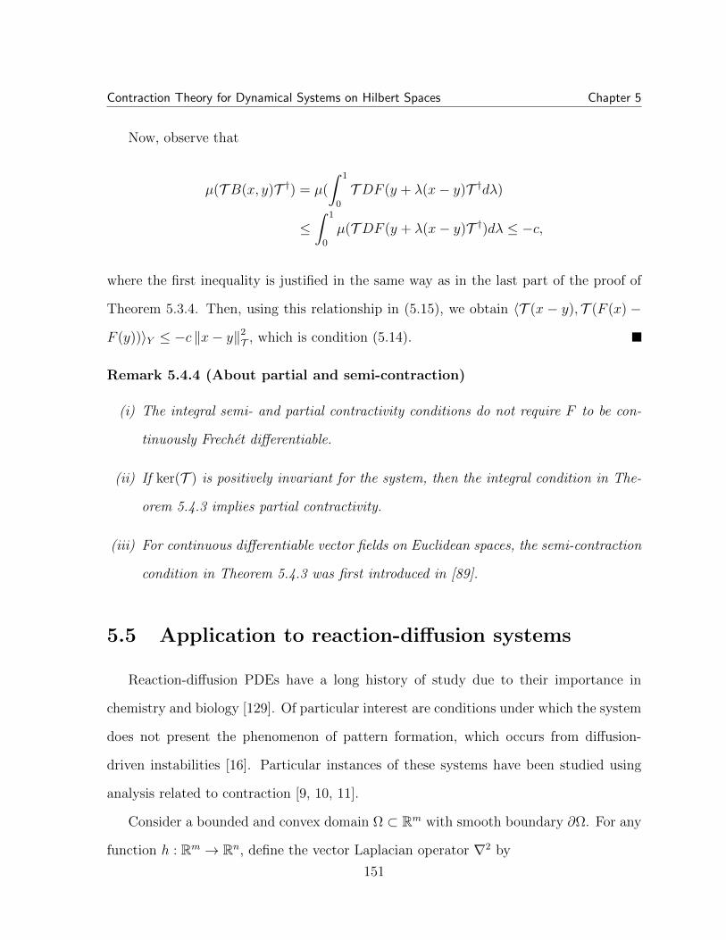
Contraction Theory for Dynamical Systems on Hilbert Spaces Chapter 5
Now, observe that
µ(T B(x, y)T †) = µ(
∫ 1
0
T DF (y + λ(x− y)T †dλ)
≤∫ 1
0
µ(T DF (y + λ(x− y)T †)dλ ≤ −c,
where the first inequality is justified in the same way as in the last part of the proof of
Theorem 5.3.4. Then, using this relationship in (5.15), we obtain 〈T (x − y), T (F (x) −
F (y))〉Y ≤ −c ‖x− y‖2T , which is condition (5.14).
Remark 5.4.4 (About partial and semi-contraction)
(i) The integral semi- and partial contractivity conditions do not require F to be con-
tinuously Frechet differentiable.
(ii) If ker(T ) is positively invariant for the system, then the integral condition in The-
orem 5.4.3 implies partial contractivity.
(iii) For continuous differentiable vector fields on Euclidean spaces, the semi-contraction
condition in Theorem 5.4.3 was first introduced in [89].
5.5 Application to reaction-diffusion systems
Reaction-diffusion PDEs have a long history of study due to their importance in
chemistry and biology [129]. Of particular interest are conditions under which the system
does not present the phenomenon of pattern formation, which occurs from diffusion-
driven instabilities [16]. Particular instances of these systems have been studied using
analysis related to contraction [9, 10, 11].
Consider a bounded and convex domain Ω ⊂ Rm with smooth boundary ∂Ω. For any
function h : Rm → Rn, define the vector Laplacian operator ∇2 by
151

Contraction Theory for Dynamical Systems on Hilbert Spaces Chapter 5
∇2h = (∇2h1, . . . ,∇2hn)> and (∇2h(x))i =∑n
j=1∂2hi(x)
∂x2j
. Let L2(Ω) be the space of
squared-integrable functions h : Ω ⊂ Rm → Rn with∫
Ωh2i dx < ∞, i ∈ 1, . . . , n,
endowed with inner product 〈u, v〉 =∫
Ωu>vdx for any u, v ∈ L2(Ω) and induced norm
‖u‖ =√〈u, u〉. It is known that (L2(Ω), 〈·, ·〉) is a Hilbert space.
Given a continuously differentiable reaction function f : Rn → Rn and a nonnegative
matrix of diffusion rates Γ ∈ Rn×n, the reaction-diffusion system with Neumann boundary
conditions is∂u
∂t= f(u) + Γ∇2u
∇ui(x) · n(x) = 0 for all x ∈ ∂Ω, i1, . . . , n,(5.16)
for u ∈ L2(Ω) and (t, x) ∈ R≥0 × Ω. We refer to [16] and references therein for the
system’s well-posedness and existence of classical solutions u = u(x, t) such that u(t, ·)
is twice continuously differentiable for each fixed t ∈ R≥0, and that t 7→ u(t, ·) is a twice
continuously differentiable function on Ω. We assume that classical solutions exist.
A Neumann eigenvalue λ ∈ R for the Laplacian operator ∇2 on Ω is defined by
−∇2u = λu
∇ui(x) · n(x) = 0 for all x ∈ ∂Ω, i ∈ 1, . . . , n.
The set of Neumann eigenvalues of the Laplacian operator consists of countably many
nonnegative values with no finite accumulation point [79, Section 7.1]. For our Ω, the
eigenspace associated with the lowest eigenvalue λ = 0 is
S = h ∈ L2(Ω) | h(x) = c for all x ∈ Ω
and some constant vector c.(5.17)
The volume of Ω is |Ω| =∫
Ωdx and the spatial average of h ∈ L2(Ω) over Ω is h =
152

Contraction Theory for Dynamical Systems on Hilbert Spaces Chapter 5
1|Ω|
∫Ωh(x)dx ∈ Rn. Define the operator ΠS : L2(Ω)→ S⊥ by
ΠS(u) = u− u. (5.18)
One can easily check that ΠS is the orthogonal projection onto S⊥. Since ΠS is surjective,
i.e., im(ΠS) = S⊥, it follows from the definition of the Moore-Penrose pseudoinverse and
its uniqueness that Π†S : S⊥ → L2(Ω) is given by Π†S(u) = u.
Given a matrix A ∈ Rn×n, the matrix measure associated to the standard Euclidean
2-norm, µ2(A), has the following property [11]: µ2(A) ≤ c if and only if A+A>
2 cIn, i.e.,
cIn − A+A>
2is positive semi-definite.
Theorem 5.5.1 (Partial and semi-contraction of reaction-diffusion systems) Let
the reaction-diffusion system (5.16) with the standard assumptions on f , Γ, and over a
bounded and convex set domain Ω ⊂ Rm. Suppose that there exists a positive definite
matrix P ∈ Rn×n such that µ2(PΓ) ≥ 0 and µ2(P (Df(x)−λ2Γ)) ≤ −c for all x ∈ Ω and
some constant c > 0. Define u 7→ ‖u‖ΠS ,P 1/2 :=∥∥ΠS(P 1/2u)
∥∥ with the set S as in (5.17),
and let λmax(P ) be the largest eigenvalue of P . Then,
(i) system (5.16) is partially contractive with respect to ‖·‖ΠS ,P 1/2, that is, for every
solution u : R≥0 × Ω→ Rn,
‖u(t, ·)‖ΠS ,P 1/2 ≤ e−c
λmax(P ) ‖u(0, ·)‖ΠS ,P 1/2 ,
(ii) ker(ΠS) = S is an invariant subspace and all trajectories exponentially converge to
it; and
(iii) if additionally f(u) = Au, A ∈ Rn×n, then (5.16) is semi-contractive with respect
153

Contraction Theory for Dynamical Systems on Hilbert Spaces Chapter 5
to ‖·‖ΠS ,P 1/2, that is, for every solution u, v : R≥0 × Ω→ Rn,
‖u(t, ·)− v(t, ·)‖ΠS ,P 1/2 ≤ e−c
λmax(P ) ‖u(0, ·)− v(0, ·)‖ΠS ,P 1/2 ,
Proof: Note that the reaction-diffusion system we are analyzing can be written
as ∂u∂t
= F (u) where F : L2(Ω) → L2(Ω) is defined by F (u) := f(u) + Γ∇2u. Let
〈·, ·〉ΠS ,P 1/2 := 〈ΠS(P 1/2·),ΠS(P 1/2·)〉.
We start by proving statement (i). Consider any u ∈ L2(Ω), and set u = u − u, so
that u ∈ S⊥. Then,
〈u, F (u)〉ΠS ,P 1/2 = 〈u, f(u)〉ΠS ,P 1/2 + 〈u,Γ∇2(u)〉ΠS ,P 1/2 (5.19)
First, from the first term in the right-hand side of (5.19),
〈u, f(u)〉ΠS ,P 1/2 = 〈ΠS(P 1/2(u)),ΠS(P 1/2(f(u)))〉
=
∫
Ω
u>P (f(u)− f(u))dx
=
∫ 1
0
∫
Ω
u>PDf(s(λ))udxdλ.
(5.20)
where for the second equality we repeatedly used∫
Ωu>adx = 0 for any constant vec-
tor a ∈ Rn in Ω, and, since Ω is convex, the mean-value theorem: f(u) − f(u) =∫ 1
0Df(s(λ))udλ with s(λ) = u + λ(u− u) for the last inequality. Now, from the second
term in the right-hand side of (5.19),
〈u,Γ∇2u〉ΠS ,P 1/2 =
∫
Ω
u>PΓ∇2udx, (5.21)
where we used ΠS(∇2u) = ∇2u− 1|Ω|
∫Ω∇2udx = ∇2u, since
∫Ω∇2uidx =
∫∂Ω∇ui · ndS =
0 (from the divergence theorem and the boundary condition in (5.16)). Note that, for
154

Contraction Theory for Dynamical Systems on Hilbert Spaces Chapter 5
every i ∈ 1, . . . , n, we have ∇2ui(x) = ∇ · (∇ui(x)). Now, by the product rule, we
have that for every i ∈ 1, . . . , n, ∇ · (∑n
j=1 ui(PΓ)ij∇uj) =∑n
j=1 ui(PΓ)ij∇2uj +∑n
j=1(∇ui)>(PΓ)ij∇uj. Now, by the divergence theorem, we obtain for every i ∈
1, . . . , n,∫
Ω∇ · (∑n
j=1 ui(PΓ)ij∇uj)dx =∫∂Ω
(∑nj=1 ui(PΓ)ij∇uj · n
)dS = 0 where
the last equality follows from the boundary condition in (5.16). Then, from the identity
u>PΓ∇2u =∑n
i=1
∑nj=1 ui(PΓ)ij∇2uj we get
∫
Ω
u>PΓ∇2udx = −∫
Ω
n∑
i=1
n∑
j=1
(∇ui)>(PΓ)ij∇ujdx.
Moreover, one can check that
n∑
i=1
n∑
j=1
(∇ui)>(PΓ)ij∇uj =n∑
k=1
(∂u
∂xk)>(PΓ)
∂u
∂xk.
Since µ2(PΓ) ≥ 0, there exists a positive semi-definite matrix Q ∈ Rn×n such that
Q>Q = 12(PΓ + Γ>P>). This implies that
∑nk=1( ∂u
∂xk)>PΓ ∂u
∂xk=∑n
k=1( ∂u∂xk
)>Q>Q ∂u∂xk
=∑n
k=1(∂Qu∂xk
)> ∂Qu∂xk
=∑n
i=1(∇((Qu)i))>∇((Qu)i).
Combining all of these results, we finally obtain∫
Ωu>PΓ∇2udx = −∑n
i=1 ‖∇(Qu)i‖2.
Now, since∫
ΩQudx = Q
∫Ωudx = 0n, we can use the Poincare inequality on simply con-
nected domains [79, Section 1.3] (since our domain is convex), and obtain ‖∇(Qu)i‖2 ≥
λ2‖(Qu)i‖2. As a result, we get
∫
Ω
u>PΓ∇2udx ≤ −λ2
n∑
i=1
‖(Qu)i‖2 =
∫
Ω
u> (−λ2PΓ) udx.
Replacing this result in (5.21), and then replacing the resulting expression with the one
155

Contraction Theory for Dynamical Systems on Hilbert Spaces Chapter 5
in (5.20) back in (5.19):
〈u, F (u)〉ΠS ,P 1/2 =
∫ 1
0
∫
Ω
u>P (Df(s(λ))− λ2Γ) udxdλ
≤ −c∫ 1
0
∫
Ω
u>udxdλ ≤ − c
λmax(P )
∥∥P 1/2u∥∥
= − c
λmax(P )‖u‖ΠS,P 1/2 = − c
λmax(P )‖u‖ΠS,P 1/2
where the inequality comes from the assumption µ2(P (Df(x)−λ2Γ)) ≤ −c for any x ∈ Ω.
This expression has the form of the integral partial contractivity condition. Although
the set of classical solutions endowed with 〈·, ·〉 is not a Hilbert space, we follow the
proof of Theorem 5.4.2 using the Leibniz rule to differentiate the inner product and
obtain partial contraction as in statement (i). Statement (ii) follows by noting that
‖u‖ΠS ,P 1/2 = 0 =⇒ P 1/2u ∈ ker(ΠS) =⇒ P 1/2u ∈ S =⇒ u ∈ S. Finally,
statement (iii) is proved in a similar way to statement (i), using the difference of any two
solutions as a new state variable.
Remark 5.5.2 Statements (i) and (ii) of Theorem 5.5.1 are essentially the same result
as [16, Theorem 1]; however, these statements and statement (iii) are now consequences
of a general contraction theory.
5.6 Conclusion
This paper presents a general contraction theory for dynamical systems on Hilbert
spaces. We provide sufficient conditions for contraction, semi-contraction and partial
contraction based on operator measures or operator semi-measures, and on the differ-
entiability of the vector field. Moreover, when the system is time-invariant, we present
weaker conditions that do not require differentiability. Finally, we present an example of
156

Contraction Theory for Dynamical Systems on Hilbert Spaces Chapter 5
reaction-diffusion systems.
Our work brings the machinery of contraction theory, so far mainly applied to ODEs,
to other possible application domains related to a variety of systems that can be expressed
as dynamical systems on functional spaces.
157

Chapter 6
Distributed and time-varying
primal-dual dynamics via
contraction analysis
6.1 Introduction
Problem statement and motivation Primal-dual (PD) dynamics are dynamical sys-
tems that solve constrained optimization problems. Their study can be traced back to
many decades ago [18] and has regained interest since the last decade [66]. PD dynam-
ics have been made popular due to their scalability and simplicity. They have been
widely adopted in engineering applications such as resource allocation problems in power
networks [158], frequency control in micro-grids [116], solvers for linear equations [174],
etc. In this note, we study optimization problems with linear equality constraints. In
general, PD dynamics seek to find a saddle point of the associated Lagrangian function
to the constrained problem, which is characterized by the equilibria of the dynamics.
For a general treatise of asymptotic stability of saddle points, we refer to [42] and refer-
158

Distributed and time-varying primal-dual dynamics via contraction analysis Chapter 6
ences therein. However, despite the long history of study and application, there are very
recent studies on PD dynamics related to linear equality constraints further studying
different dynamic properties such as: exponential convergence under different convexity
assumptions [145, 40] and contractivity properties [132].
We are particularly interested in studying primal-dual dynamics in distributed and
time-varying optimization problems. We refer to the recent survey [176] for an overview
of the long-standing interest on distributed optimization. Of particular interest is to
provide strong convergence guarantees such as global (and exponential) convergence for
the distributed solvers. We aim to provide them using contraction theory. Time-varying
optimization has found applications in system identification, signal detection, robotics,
traffic management, etc. [65, 160]. The goal is to employ a dynamical system able to track
the time-varying optimal solution up to some bounded error in real time. Although dif-
ferent dynamics have been proposed to both time-varying centralized [65] and distributed
problems [160, 148], to the best of our knowledge, there has not been a characterization
of the PD dynamics in such application contexts. The importance of PD algorithms is
their simplicity of implementation, i.e., they do not require more complex information
structures like the inverse of the Hessian of the system at all times, as in [65] and [148] for
the centralized and distributed cases respectively. However, simplicity may come with a
possible trade-off in the tracking error.
Contraction is valuable in practice because it introduces strong stability and robust-
ness guarantees. For example, it implies input-to-state stability for systems subject to
state-independent disturbances. It also guarantees fast correction after transient pertur-
bations to the trajectory of the solution, since initial conditions are forgotten. Moreover,
a contractive system may be robust towards structural perturbations on the vector field,
e.g., when a non-convex term is added to the objective function. Finally, contraction
guarantees stable numerical discretizations with geometric convergence rates, an ideal
159

Distributed and time-varying primal-dual dynamics via contraction analysis Chapter 6
situation for practical implementations. All these properties are transparent to whether
the system is time-varying or not. All of this motivates a contraction analysis of PD
algorithms in contrast to the prevalent Lyapunov or invariance analysis in the literature.
Literature review The recent works [145, 132, 40] study convergence properties of PD
dynamics under different assumptions on the objective function. In distributed optimiza-
tion, solvers based on PD dynamics are fairly recent, e.g., [173, 49, 176]. An application
of distributed optimization of current interest - as seen in the recent survey [174] - is the
distributed least-squares problem for solving an over-determined system of linear equa-
tions. To the best of our knowledge, solvers for this problem (in continuous-time) with
exponential global convergence are still missing in the literature.
Finally, this paper is related to contraction theory, a mathematical tool to analyze
incremental stability [112, 168]. An introduction and survey can be found in [11]. A
variant of contraction theory, partial contraction [142, 59], analyzes the convergence
to linear subspaces and has been used in the synchronization analysis of diffusively-
coupled network systems [142, 12]; however, its application to distributed algorithms is
still missing, and our paper provides such contribution.
Contributions In this paper we consider the PD dynamics associated to optimization
problems with a twice differentiable and strongly convex objective function and linear
equality constraints. We use contraction theory to perform an overarching study of PD
dynamics in a variety of implementations and applications. In particular:
(i) We introduce new theoretical results of how weak and partial contraction can
imply exponential convergence to a point in a subspace of equilibria.
(ii) For the standard and distributed PD dynamics, we prove: 1) convergence under
weak contraction when the objective function is convex; 2) contraction for the standard
160

Distributed and time-varying primal-dual dynamics via contraction analysis Chapter 6
problem and partial contraction for the distributed one in the strongly convex case, with
closed-form exponential global convergence rates. The analysis in result 1) is novel,
since it uses the new results introduced in (i). Compared to the work [132] that also
shows contraction for the standard PD, our proof method provides an explicit closed-form
expression of the system’s contraction rate. Our exponential convergence rate is different
from the one by [145] via Lyapunov analysis, and both rates cannot be compared without
extra assumptions on the numerical relationships among various parameters associated
to the objective function or constraints. Moreover, we propose using the augmented
Langrangian in order to achieve contraction when the objective function is only convex.
In the case of distributed optimization, there exist other solvers that show exponential
convergence, e.g., as in [96, 105], but none of these have contractivity.
(iii) We propose a new solver for the distributed least-squares problem based on PD
dynamics, and use our results in (ii) to prove its convergence. Compared to the recent
work [110], our new model exhibits global convergence; and compared to the recent
work [111], ours exhibits exponential convergence and has a simpler structure.
(iv) We characterize the performance of PD dynamics associated to time-varying
versions of both standard and distributed optimization problems in terms of the problems’
parameters - to the best of our knowledge, this is the first characterization of time-varying
PD dynamics in the literature. We prove the tracking error to the time-varying solutions
is uniformly ultimately bounded (UUB) in either case and that the bound decreases
as the contraction rate increases. Our analysis builds upon the contraction results in
contribution (ii).
Paper organization Section 6.2 has notation and preliminary concepts. Section 6.3
has results on contraction theory. Section 6.4 analyzes contractive properties of the
standard PD dynamics. The contractive analysis of distributed (with the least-squares
161

Distributed and time-varying primal-dual dynamics via contraction analysis Chapter 6
problem application) and time-varying versions of PD dynamics are in Sections V and VI
respectively. Section 6.7 is the conclusion.
6.2 Preliminaries and notation
6.2.1 Notation, definitions and useful results
Consider A ∈ Rn×n, then σmin(A) denote its minimum singular value and σmax(A) its
maximum one. If A has only real eigenvalues, let λmax(A) be its maximum eigenvalue. A
is an orthogonal projection if it is symmetric and A2 = A. Let ‖·‖ denote any norm, and
‖·‖p denote the `p-norm. When the argument of a norm is a matrix, we refer to its respec-
tive induced norm. The matrix measure associated to ‖·‖ is µ(A) = limh→0+‖I+hA‖−1
h;
e.g., the one associated to the `2-norm is µ2(A) = λmax((A + A>)/2) [11]. Given invert-
ible Q ∈ Rn×n, let ‖·‖2,Q be the weighted `2-norm ‖x‖2,Q = ‖Qx‖2, x ∈ Rn, and whose
associated matrix measure is µ2,Q(A) = µ2(QAQ−1) [11].
Let In be the n × n identity matrix, 1n and 0n be the all-ones and all-zeros column
vector with n entries respectively. Let diag(X1, . . . , XN) ∈ R∑Ni=1 ni×
∑Ni=1 ni be the block-
diagonal matrix with elements Xi ∈ Rni×ni . Let R≥0 be the set of non-negative real
numbers. Given xi ∈ Rki , let (x1, . . . , xN) =
[x>1 . . . x>N
].
Consider a differentiable function f : Rn → Rn. We say f is Lipschitz smooth with
constant K1 > 0 if ‖∇f(x)−∇f(y)‖2 ≤ K1 ‖x− y‖2 for any x, y ∈ Rn; and strongly
convex with constant K2 > 0 if K2 ‖x− y‖22 ≤ (∇f(x)−∇f(y))>(x−y) for any x, y ∈ Rn.
Assuming f is twice differentiable, these two conditions are equivalent to ∇2f(x) K1In
and K2In ∇2f(x) for any x ∈ Rn, respectively.
The proof of the next proposition is found in the Appendix.
162

Distributed and time-varying primal-dual dynamics via contraction analysis Chapter 6
Proposition 6.2.1 For a full-row rank matrix A ∈ Rm×n, B = B> ∈ Rn×n, and b2 ≥
b1 > 0 such that b2In B b1In 0, the matrix
−B −A>
A 0m×m
is Hurwitz.
6.2.2 Review of basic concepts on contraction theory
Consider the dynamical system x = f(x, t) with x ∈ Rn. Let t 7→ φ(t, t0, x0) be the
trajectory of the system starting from x0 ∈ Rn at time t0 ≥ 0. Consider the system
satisfies ‖φ(t, t0, x0)− φ(t, t0, y0)‖ ≤ ‖x0 − y0‖ e−c(t−t0), for any x0, y0 ∈ Rn and any
t0 ∈ R≥0. We say it is contractive with respect to ‖·‖ when c > 0, and weakly contractive
when c = 0. A time-invariant contractive system has a unique equilibrium point. Now,
assume the Jacobian of the system, i.e., Df(x, t), satisfies: µ(Df(x, t)) ≤ −c for any
(x, t) ∈ Rn×R≥0, with µ being the matrix measure associated to ‖·‖ and constant c ≥ 0.
Then, this system has contraction rate c with respect to ‖·‖. Now, assume the system has
a flow-invariant linear subspace M = x ∈ Rn | V x = 0k with V ∈ Rk×n being full-row
rank with orthonormal rows. Then the system is partially contractive with respect to ‖·‖
andM if there exists c > 0 such that, for any x0 ∈ Rn and t0 ∈ R≥0, the system satisfies
‖V φ(t, t0, x0)‖ ≤ ‖V x0‖ e−c(t−t0). When c = 0, the system is partially weakly contractive
with respect to M [142]. Consequently, a partially contractive system has any of its
trajectories approaching M with exponential rate; and a partially weakly contractive
one has any of its trajectories at a non-increasing distance from M.
Pick a symmetric positive-definite P ∈ Rn×n and a scalar c > 0, then µ2,P 1/2(Df(x, t)) ≤
−c for all (x, t) ∈ Rn×R≥0 is equivalent to f satisfying the integral contractivity condition,
i.e., for every x, y ∈ Rn and t ≥ 0, (y − x)>P (f(x, t)− f(y, t)) ≤ −c ‖x− y‖22,P 1/2 .
163

Distributed and time-varying primal-dual dynamics via contraction analysis Chapter 6
6.3 Theoretical contraction results
The next result will be used throughout the paper.
Theorem 6.3.1 (Results on partial contraction) Consider the system x = f(x, t),
x ∈ Rn, with a flow-invariant M = x ∈ Rn | V x = 0k with V ∈ Rk×n being a full-row
rank matrix with orthonormal rows. Assume µ(V Df(x, t)V >) ≤ −c for any (x, t) ∈
Rn × R≥0, some constant c ≥ 0 and some matrix measure µ.
(i) If c > 0, then the system is partially contractive with respect to M and every
trajectory exponentially converges to the subspace M with rate c.
(ii) If c = 0 and µ(V Df((In − V >V )x, t)V >) < 0 for any (x, t) ∈ Rn × R≥0, then
the system is partially weakly contractive with respect to M and every trajectory
converges to the subspace M.
Moreover, assume that one of the conditions in parts (i) and (ii) holds and M is a set
of equilibrium points. If the system is weakly contractive, then
(iii) every trajectory of the system converges to an equilibrium point, and if c > 0, then
it does it with exponential rate c.
Remark 6.3.2 Statement (i) in Theorem 6.3.1 was proved in [142]. To the best of our
knowledge, statements (ii) and (iii) are novel.
Proof: [Proof of Theorem 6.3.1] It is easy to check that V >V is an orthogonal
projection matrix onto M⊥; and that U := In − V >V is also an orthogonal projection
matrix onto M. Using these results, we can express the given system as x = f(Ux +
V >V x, t). Now, we set z := V x, and observe that x(t) converges toM if and only if z(t)
converges 0k. Then, using this change of coordinates, we obtain the system:
z = V f(Ux+ V >z, t). (6.1)
164

Distributed and time-varying primal-dual dynamics via contraction analysis Chapter 6
It has been proved in [142, Theorem 3] that z∗ = 0k is an equilibrium point for the
system (6.1).
To prove (ii), assume that µ(V Df(x, t)V >) = 0 for any (x, t) ∈ Rn × R≥0; i.e., that
the system (6.1) is weakly contractive. Now, if we assume that µ(V Df(Ux, t)V >) < 0
for any (x, t) ∈ Rn×R≥0, then by the Coppel’s inequality [48], the fixed point z∗ = 0k is
locally exponentially stable. Now, we can use a generalization of [113, Lemma 6], namely
Lemma 6.8.1 (proof found in the Appendix), to establish the convergence of z(t) to z∗.
This finishes the proof for (ii).
Now, we prove statement (iii). Let t 7→ x(t) be a trajectory of the dynamical system.
For every t ∈ R≥0,(In−V >V
)x(t) is the orthogonal projection of x(t) onto the subspace
M and it is an equilibrium point. Since the dynamical system is weakly contractive, we
have ‖x(s) − (In − V >V )x(t)‖ ≤ ‖x(t) − (In − V >V )x(t)‖ = ‖V >V x(t)‖, for all s ≥ t.
This implies that, for every t ∈ R≥0 and every s ≥ t, the point x(s) remains inside the
closed ball B(x(t), ‖V >V x(t)‖). Therefore, for every t ≥ 0, the point x(t) is inside the set
Ct defined by Ct = cl(⋂
τ∈[0,t] B(x(τ), ‖V >V x(τ)‖)). It is easy to see that, for s ≥ t, we
have Cs ⊆ Ct. This implies that the family Ctt∈[0,∞) is a nested family of closed subsets
of Rn. Moreover, by parts (i) and (ii), we have that limt→∞ ‖V >V x(t)‖ → 0 as t → ∞,
which in turn results in limt→∞ diam(Ct) = 0, with convergence rate c for the case c > 0
because of diam(Ct) = ‖V >V x(t)‖ ≤ 2e−ct‖V >V x(0)‖. Thus, by the Cantor Intersection
Theorem [128, Lemma 48.3], there exists x∗ ∈ Rn such that⋂t∈[0,∞) Ct = x∗. We first
show that limt→∞ x(t) = x∗. Note that x∗, x(t) ∈ Ct, for every t ∈ R≥0. This implies
that ‖x(t) − x∗‖ ≤ diam(Ct). This in turn means that limt→∞ ‖x(t) − x∗‖ = 0 and
t 7→ x(t) converges to x∗, with convergence rate c for the case c > 0. On the other hand,
by part (i), the trajectory t 7→ x(t) converges to the subspace M. Therefore, x∗ ∈ M
and x∗ is an equilibrium point of the dynamical system. This completes the proof for
statement (iii).
165

Distributed and time-varying primal-dual dynamics via contraction analysis Chapter 6
6.4 The standard optimization problem
We consider the constrained optimization problem:
minx∈Rn
f(x) subject to Ax = b (6.2)
with the following standing assumptions: A ∈ Rk×n, k < n, b ∈ Rk, A is full-row rank,
and f : Rn → R is convex and twice differentiable.
Associated to the optimization problem (6.2) is the Lagrangian function L(x, ν) =
f(x) + ν>(Ax− b) and the primal-dual dynamics
x
ν
=
−∂L(x,ν)
∂x
∂L(x,ν)∂ν
=
−∇f(x)− A>ν
Ax− b
. (6.3)
We introduce two possible sets of assumptions:
(A1) the primal-dual dynamics (6.3) have an equilibrium (x∗, ν∗) and ∇2f(x∗) 0n×n;
(A2) the function f is strongly convex with constant `inf > 0 and Lipschitz smooth with
constant `sup > 0, and, for 0 < ε < 1, we define
αε :=ε`inf
σ2max(A) + 3
4σmax(A)σ2
min(A) + `2sup
> 0
P :=
In αε A
>
αε A Ik
∈ R(n+k)×(n+k).
(6.4)
Theorem 6.4.1 (Contraction analysis of primal-dual dynamics) Consider the con-
strained optimization problem (6.2), its standing assumptions, and its associated primal-
dual dynamics (6.3).
166

Distributed and time-varying primal-dual dynamics via contraction analysis Chapter 6
(i) The primal-dual dynamics is weakly contractive with respect to ‖·‖2 and, if Assump-
tion (A1) holds, then (x∗, ν∗) is globally asymptotically stable.
(ii) Under Assumption (A2),
(a) the primal-dual dynamics are contractive with respect to ‖·‖2,P 1/2 with contrac-
tion rate
αε3
4
σmax(A)σ2min(A)
σmax(A) + 1, and (6.5)
(b) there exists a unique globally exponentially stable equilibrium point (x∗, ν∗),
and x∗ is the unique solution to the optimization problem (6.2).
Proof: Let (x, ν)> := FPD(x, ν). Then, DFPD(x, ν) =
−∇2f(x) −A>
A 0
, and so
µ2(DFPD(x, ν)) = λmax
((DFPD(x, v) +DFPD(x, v)>)/2
)= λmax (diag(−∇2f(x), 0k×k)) =
0 for any (x, ν) ∈ Rn × Rm, because of convexity ∇2f(x) 0, which implies the system
is weakly contractive. For the second part of statement (i): Proposition 6.2.1 implies
DFPD(x∗, ν∗) is Hurwitz since ∇2f(x∗) 0, and the proof follows from a simple gener-
alization of [113, Lemma 6] (its proof can be found in the Appendix).
Now, we prove statement (ii). Define P =
In αA>
αA Ik
which is a positive-definite
matrix when
0 < α <1
σmax(A). (6.6)
We plan to use the integral contractivity condition to show that system (6.3) is contractive
with respect to norm ‖·‖2,P 1/2 . Thus, we need to show
η :=
x1 − x2
ν1 − ν2
>
P (FPD(x1, ν1)− FPD(x2, ν2)) + c
x1 − x2
ν1 − ν2
>
P
x1 − x2
ν1 − ν2
≤ 0
167

Distributed and time-varying primal-dual dynamics via contraction analysis Chapter 6
for any x1, x2 ∈ Rn and ν1, ν2 ∈ Rm, and some constant c > 0 which will be the contrac-
tion rate. After completing squares, using the strong convexity and Lipschitz smoothness
of f , along with σ2min(A)Ik AA> and A>A σ2
max(A)In, we obtain
η ≤ −((3α/4)σ2
min(A)− c− cα)‖ν1 − ν2‖2
2 − (`inf
− ασ2max(A)− c− α`2
sup − cασ2max(A)) ‖x1 − x2‖2
2
− αc ‖(ν1 − ν2)− A(x1 − x2)‖22 .
Set c = Dα for some D > 0. Then, to ensure that η ≤ 0, we need to ensure
3α
4σ2
min(A)−Dα−Dα2 ≥ 0, (6.7)
`inf − ασ2max(A)−Dα− α`2
sup −Dα2σ2max(A) ≥ 0. (6.8)
Now, to ensure inequality (6.7) holds, using the inequalities (6.6), it is easy to see that
it suffices to ensure that
3σmax(A)σ2min(A)
4(σmax(A) + 1)> D. (6.9)
Now, using inequalities (6.6) and (6.9), we obtain: `inf − ασ2max(A) − Dα − α`2
sup −
Dα2σ2max(A) > `inf − α(σ2
max(A) + 34σmax(A)σ2
min(A) + `2sup) and so, to ensure inequal-
ity (6.8) holds, it suffices that
`inf
σ2max(A) + 3
4σmax(A)σ2
min(A) + `2sup
> α. (6.10)
Now, the parameter α needs to satisfy inequalities (6.6) and (6.10); however, (6.10)
implies (6.6) because the inequality π21 + π2
2 ≥ 2π1π2 for π1, π2 > 0 let us conclude that
`sup
σ2max(A)+`2sup
≤ 12σmax(A)
. Finally, c must be less than the multiplication of the left-hand
sides of the inequalities (6.9) and (6.10), which proves statement (ii)a.
168

Distributed and time-varying primal-dual dynamics via contraction analysis Chapter 6
Now, since the dynamics are contractive, there must exist a unique globally expo-
nentially stable equilibrium point which also satisfies the (sufficient and necessary) KKT
conditions of optimality for the optimization problem (6.2), thus proving statement (ii)b.
Remark 6.4.2 Theorem 6.4.1 is a fundamental building block for the rest of results in
the results in this paper and therefore, it was necessary to provide a comprehensive proof
using the integral contractivity condition that could provide an explicit estimate of the
contraction rate (as opposed to the different proof in [132]).
For the case of convex f , Theorem 6.4.1 does not state convergence - nor contraction
- without additional assumptions; indeed, oscillations may appear and convergence to
the saddle points is not guaranteed [66]. In order to still be able to use Theorem 6.4.1
in this case, we consider a modification to the Lagrangian, known as the augmented
Lagrangian [149]: Laug(x, ν) = L(x, ν) + ρ2‖Ax− b‖2
2 with gain ρ > 0. Its associated
augmented primal-dual dynamics become
x
ν
=
−∇f(x)− A>ν − ρA>Ax+ ρA>b
Ax− b
(6.11)
and have the same equilibria as the original one in (6.3). We introduce two possible sets
of assumptions:
(A3) the primal-dual dynamics (6.3) have an equilibrium (x∗, ν∗), ∇2f(x∗) 0n×n, and
ker(∇2f(x∗)) ∩ ker(A) = 0n;
(A4) ker(∇2f(x)) ∩ ker(A) = 0n for any x ∈ Rn and f is Lipschitz smooth with
constant `sup > 0, and, for 0 < ε < 1, we define
169

Distributed and time-varying primal-dual dynamics via contraction analysis Chapter 6
αε :=ερσ2
min(A)
(1 + ρ)σ2max(A) + 3
4σmax(A)σ2
min(A) + `2sup
P :=
In αε A
>
αε A Ik
∈ R(n+k)×(n+k).
(6.12)
Corollary 6.4.3 (Contraction analysis of the augmented primal-dual dynamics)
Consider the constrained optimization problem (6.2), its standing assumptions, and its
associated augmented primal-dual dynamics (6.11) with ρ > 0.
(i) Under Assumption (A3), the augmented primal-dual dynamics are weakly contrac-
tive with respect to ‖·‖2 and (x∗, ν∗) is globally asymptotically stable.
(ii) Under Assumption (A4),
(a) the augmented primal-dual dynamics are contractive with respect to ‖·‖2,P 1/2
with contraction rate
αε3
4
σmax(A)σ2min(A)
σmax(A) + 1, and (6.13)
(b) there exists a unique globally exponentially stable equilibrium point (x∗, ν∗)
for the augmented primal-dual dynamics and x∗ is the unique solution to the
constrained optimization problem (6.2).
Proof: The proof follows directly from Theorem 6.4.1. For statement (i), note that
ker(∇2f(x∗)) ∩ ker(A) = 0n implies that ∇2f(x∗) + ρA>A 0n×n for the Jacobian of
the system −∇2f(x)− ρA>A −A>
A 0
.
170

Distributed and time-varying primal-dual dynamics via contraction analysis Chapter 6
For statement (ii), note that ker(∇2f(x)) ∩ ker(A) = 0n for any x ∈ Rn implies that
x 7→ f(x)+ ρ2x>A>Ax is Lipschitz smooth with constant `2
sup+ρσ2max(A) > 0 and strongly
convex with constant ρσ2min(A) > 0.
Remark 6.4.4 (Augmented Lagrangian and contraction) The benefit of using the
augmented Lagrangian is that, unlike the conditions in Theorem 6.4.1, the primal-dual
dynamics may be contractive despite f being only convex.
6.5 Distributed algorithms
We study a popular distributed implementation for solving an unconstrained opti-
mization problem [176]. We want to solve the problem minx∈Rn f(x) =∑N
i=1 fi(x) with
fi : Rn → R convex. Let G be an undirected connected interaction graph between N
distinct agents. Let Ni be the neighborhood of node i and L be the Laplacian matrix of
G. Let xi ∈ Rn be the state associated to agent i, and let x = (x1, . . . , xN)>. Then, the
problem becomes:
minx∈RnN
N∑
i=1
fi(xi)
(L⊗ In)x = 0nN
. (6.14)
The associated distributed primal-dual dynamics are
xi = −∇xifi(xi)−
∑
j∈Ni
(νj − νi)
νi =∑
j∈Ni
(xj − xi)(6.15)
for i ∈ 1, . . . , N. In system (6.15), any agent only uses information from herself and
the set of her neighbors.
171

Distributed and time-varying primal-dual dynamics via contraction analysis Chapter 6
To study this system, we introduce two possible sets of assumptions:
(A5) minx∈Rn f(x) has a solution x∗ and ∇2fi(x∗) 0n×n for any i ∈ 1, . . . , N;
(A6) minx∈Rn f(x) has a solution x∗ and the function fi is strongly convex with constant
`inf,i > 0 and Lipschitz smooth with constant `sup,i > 0 for any i ∈ 1, . . . , N, with
`inf = (`inf,1, . . . , `inf,N) and `sup = (`sup,1, . . . , `sup,N).
With either assumption, note that we cannot apply Theorem 6.4.1 directly since the
linear equality constraint in (6.14) is not full-row rank. However, if we instead consider
partial contraction, then Theorem 6.4.1 can be used to prove the next result.
Theorem 6.5.1 (Contraction analysis of distributed dynamics) Consider the dis-
tributed primal-dual dynamics (6.15).
(i) The distributed primal-dual dynamics are weakly contractive with respect to ‖·‖2,
and
(ii) under Assumption (A5), for any (xi(0), νi(0)) ∈ Rn × Rn, limt→∞ xi(t) = x∗ and
limt→∞ νi(t) = ν∗i , for some ν∗i such that
∑Nk=1 ν
∗k =
∑Nk=1 ν
k(0).
(iii) Under Assumption (A6), the convergence results in statement (ii) hold and, for
0 < ε < 1, the convergence of (x(t), ν(t))> has exponential rate
3ε
4
λNλ22
λN + 1
mini∈1,...,N `inf,i
λ2N + 3
4λNλ2
2 + ‖`sup‖2∞, (6.16)
where λ2 and λN are the smallest non-zero and the largest eigenvalues of L, respec-
tively.
Proof: Set f(x) =∑N
i=1 fi(xi) and ν = (ν1, . . . , νN). Succinctly, the dynamics of
172

Distributed and time-varying primal-dual dynamics via contraction analysis Chapter 6
the system are
x = −∇f(x)− (L⊗ In)ν
ν = (L⊗ In)x
. (6.17)
Now, let A := (L⊗ In) and (x, ν) := FPD-d(x, ν), and so
DFPD-d(x, ν) =
−∇2f(x) −A>
A 0m×m
.
Since −∇2f(x) 0nN×nN because of convex fi, it follows that µ2(DFPD-d(x, ν)) = 0 for
any x ∈ RnN , ν ∈ RnN , and the system is weakly contractive, which proves (i).
Consider the equilibrium equations of (6.17), and let (x∗, ν∗) be a (candidate) fixed
point of the system. From the second equation in (6.17), x∗ = 1N ⊗v with v ∈ Rn. Now,
from the first equation in (6.17), we get 0nN = ∇f(x∗) + (L⊗ In)ν∗ and left multiplying
by 1>N ⊗ In, we obtain 0n =
∑Ni=1∇fi(v). This is exactly the necessary and sufficient
conditions of optimality for the problem minx∈Rn f(x) =∑N
i=1 fi(x), and so v = x∗ is an
optimal solution to this problem. Moreover, ν∗ is just some Lagrange multiplier for the
constraint in (6.14).
Now, define the change of coordinates (x′, ν ′) = (x − x∗, ν − ν∗), then we get
(x′, ν ′) = (x, ν) = FPD-d(x′ + x∗, ν ′ + ν∗), and whenever we refer to the word “sys-
tem” for the rest of the proof, we refer to the dynamics after this coordinate change.
Observe the system has an equilibrium point (0nN , 0nN), but it is not unique; in fact,
it is easy to verify that the following is a linear subspace of equilibria for the system:
M =
(x′, ν ′) ∈ RnN × RnN | x′ = 0nN , ν′ = 1N ⊗ α with α ∈ Rn
. As a corollary, the
subspace M is flow-invariant for the distributed system.
Now, since L has N − 1 strictly positive eigenvalues, we can write them as 0 =
173

Distributed and time-varying primal-dual dynamics via contraction analysis Chapter 6
λ1 < λ2 ≤ · · · ≤ λN , and, by eigendecomposition, we can obtain an orthogonal matrix
R′ ∈ RN×N such thatR′LR′> = diag(0, λ2, . . . , λN). From here, we obtain the matrixR ∈
RN−1×N as a submatrix of R′ such that RLR> = Λ with Λ = diag(λ2, . . . , λN) with the
properties: RL = ΛR, RR> = IN−1 and R>R 6= IN . Now, define V = diag(InN , (R⊗In))
which has orthonormal rows and expresses
M =
(x′, ν ′) ∈ RnN × RnN | V (x′, ν ′)> = 0(2N−1)n
.
Then, we can use Theorem 6.3.1 for stating the convergence of trajectories of the system
to M using partial contraction. First, note that
V DFPD-d(x′, ν ′)V > =
∇2f(x′ + x∗) −((R>Λ)⊗ In)
((ΛR)⊗ In) 0n(N−1)×n(N−1)
,
where we have used the fact that (R⊗In)(L⊗In) = (ΛR)⊗In. Now, set A∗ := (ΛR)⊗Inand note that σmin(A∗) = λ2 and σmax(A∗) = λN .
Since ∇2f(x′ + x∗) 0nN×nN , it follows that µ2(V DFPD-d(x′ + x∗, ν ′ + ν∗)V >) ≤ 0.
Now, since ∇2f(x∗) ≺ 0nN×nN , Proposition 6.2.1 implies that V DFPD-d(x∗, ν∗)V > is
a Hurwitz matrix, which implies that µ2(V DFPD-d(x′ + x∗, ν ′ + ν∗)V >) < 0 for any
(x′, ν ′) ∈M, and thus result (ii) of Theorem 6.3.1 implies the convergence to the subspace
M (and this implies convergence of the trajectories of the original system to the set
M′ =
(x, ν) ∈ RnN × RnN | x = x∗, ν = 1N ⊗ α with α ∈ Rn
, i.e., M is simply the
set M′ translated or anchored to the origin). Since M is a set of equilibria for the
system and the system is weakly contractive, result (iii) of Theorem 6.3.1 concludes that
any trajectory of the system converges to some equilibrium point in M.
174

Distributed and time-varying primal-dual dynamics via contraction analysis Chapter 6
Now, observe that (1>N ⊗ In)ν = (1>NL⊗ In)x = 0n, and so the set
(x, ν) ∈ RnN × RnN | (1>N ⊗ In)ν = (1>N ⊗ In)ν(0)
is positively-invariant for (6.15). Then, it follows that∑N
k=1 νki (t) =
∑Nk=1 ν
ki (0) for any
i ∈ 1, . . . , n and any t ≥ 0. Then, since limt→∞ νi(t) < ∞, we conclude the proof for
statement (ii).
We prove statement (iii). Observe that
mini∈1,...,N `inf,i InN×nN ∇2f(x′ + x∗) maxi∈1,...,N `sup,i InN×nN and that A∗ is
full-row rank since it is easy to verify that rank(ΛR) = N − 1 and so rank((ΛR) ⊗
In) = n(N − 1). Then, for 0 < ε < 1, defining P =
InN αε A
∗>
αε A∗ In(N−1)
∈ RnN×nN and
αε :=εmini∈1,...,N `inf,i
σ2max(A∗)+ 3
4σmax(A∗)σ2
min(A∗)+‖`sup‖2∞> 0, we can use Theorem 6.4.1 to conclude that
µ2,P 1/2(V DFPD-d(x′ + x∗, ν ′ + ν∗)V >) ≤ −c with c as in equation (6.16) for any positive
ε < 1. So then, any trajectory (x′(t), ν ′(t)) exponentially converges to the subspace M
with rate c, due to statement (iii) from Theorem 6.3.1. Finally, the proof finishes by
following a similar proof to statement (ii).
For the case of convex fi, Theorem 6.5.1 does not state convergence - nor partial con-
traction - without additional assumptions. Similar to the analysis in Section 6.4, we
present an example where augmenting the Lagrangian let us use Theorem 6.5.1. We
consider the popular distributed least-squares problem [174]. Given a full-column rank
matrix H ∈ RN×n, n < N , it is known that x∗ = (H>H)−1H>z is the unique solution
to the least-squares problem minx∈Rn ‖z −Hx‖22, for z ∈ RN . An equivalent distributed
175

Distributed and time-varying primal-dual dynamics via contraction analysis Chapter 6
version is
minx∈RnN
N∑
i=1
(h>i xi − zi)2
(L⊗ In)x = 0nN
(6.18)
with h>i ∈ R1×n being the ith row of the matrix H, x = (x1, . . . , xN)> and z =
(z1, . . . , zN)>. Notice that f(x) =∑N
i=1 |h>i xi − zi|2 is convex, since
∇2f(x) = diag(h1h>1 , . . . , hNh
>N) 0nN×nN .
We propose to augment the Lagrangian with the quadratic term ρ2x>(L⊗In)x with ρ > 0
(which does not alter the original saddle points) and obtain
xi = −(h>i xi − zi)hi − ρ
∑
j∈Ni
(xj − xi)−∑
j∈Ni
(νj − νi)
νi =∑
j∈Ni
(xj − xi)(6.19)
for i ∈ 1, . . . , N. The new algorithm is distributed.
Observe that ker(diag(h1h>1 , . . . , hNh
>N)) ∩ ker(L⊗ In) = 0nN implies
`∗inf InN diag(h1h>1 , . . . , hNh
>N)+(L⊗In) for some constant `∗inf > 0. Then, the following
follows from Theorem 6.5.1.
Corollary 6.5.2 (Contraction analysis of distributed least-squares) Consider the
system (6.19), and let x∗ be the unique solution to the least-squares problem. Then, for
any (xi(0), νi(0)) ∈ Rn × Rn, limt→∞ xi(t) = x∗ and limt→∞ ν
i(t) = ν∗i for some ν∗i such
that∑N
k=1 ν∗k =
∑Nk=1 ν
k(0); and, for 0 < ε < 1, the convergence of (x(t), ν(t)) has
176

Distributed and time-varying primal-dual dynamics via contraction analysis Chapter 6
exponential rate
ε3
4
λNλ22
λN + 1
`∗inf
λ2N + 3
4λNλ2
2 +(λN + ρmaxi ‖hi‖2
2
)2
where λ2 and λN are the smallest non-zero and the largest eigenvalues of L, respectively.
6.6 Time-varying optimization
6.6.1 Time-varying standard optimization
Our results in Section 6.4 can be used to prove new results for the case where the
associated optimization problem is time-varying. Consider
minx∈Rn
f(x, t) subject to Ax = b(t) (6.20)
with the following standing assumptions: A ∈ Rk×n, k < n, b ∈ Rk, A is full-row rank,
and, for every (x, t) ∈ Rn × R≥0,
(i) x 7→ f(x, t) is twice continuously differentiable, uniformly strongly convex with
constant `inf > 0, i.e., ∇2f(x, t) `infIn; and uniformly Lipschitz smooth with
constant `sup > 0, i.e., ∇2f(x, t) `supIn;
(ii) t 7→ ∇f(x, t) and t 7→ b(t) are continuously differentiable functions.
The associated time-varying primal-dual dynamics are
x
ν
=
−∇f(x, t)− A>ν
Ax− b(t)
. (6.21)
Given a fixed time t, let x∗(t) be a solution to the program minx:Ax=b(t) f(x, t) and ν∗(t)
its associated Lagrange multiplier. From the standing assumptions and Theorem 6.4.1,
177

Distributed and time-varying primal-dual dynamics via contraction analysis Chapter 6
for any fixed t, there exists a unique optimizer (x∗(t), ν∗(t)). Then, (x∗(t), ν∗(t))t≥0 de-
fines the optimizer trajectory of the optimization problem (6.20). The following result
establishes the performance of the primal-dual dynamics in tracking the optimizer tra-
jectory.
Theorem 6.6.1 (Contraction analysis of time-varying primal-dual dynamics)
Consider the time-varying optimization problem (6.20), its standing assumptions, and its
associated primal-dual dynamics (6.21).
(i) The primal-dual dynamics are contractive with respect to ‖·‖2,P 1/2 with contraction
rate c, where P is the matrix defined in (6.4) and c is the same contraction rate as
in (6.5) of Theorem 6.4.1.
Assume that, for any t ≥ 0,∥∥∥b(t)
∥∥∥2≤ β1 and
∥∥∥∇f(x, t)∥∥∥
2≤ β2 for some positive
constants β1, β2, and let z(t) := (x(t), ν(t))> and z∗(t) := (x∗(t), ν∗(t))>.
(ii) Then,
‖z(t)− z∗(t)‖2,P 1/2 ≤(‖z(0)− z∗(0)‖2,P 1/2 − ρ
c
)e−ct +
ρ
c, (6.22)
i.e., the tracking error is uniformly ultimately bounded by ρc
with
ρ = λmax(P )
(β2
`inf
+
(σmax(A)
`inf
+ 1
)`max
σ2min(A)
(β1 +
σmax(A)
`inf
β2
)).
Proof: Let (x, ν) := FPD-tv(x, ν, t), and so DFPD-tv(x, ν, t) =
−∇2f(x, t) −A>
A 0k×k
.
Since A is constant and considering item (i) of the standing assumptions, we can finish
the proof for statement (i) by following the same proof as in Theorem 6.4.1. Now we prove
178

Distributed and time-varying primal-dual dynamics via contraction analysis Chapter 6
statement (ii). Let us fix any t ≥ 0. Then, the KKT conditions that the optimizers x∗(t)
and ν∗(t) must satisfy (i.e., equivalent to the equilibrium equations of the system (6.21))
are
0n = −∇f(x∗(t), t)− A>ν∗(t) (6.23)
0k = Ax∗(t)− b(t), (6.24)
We first show that the curves t 7→ x∗(t) and t 7→ ν∗(t) are continuously differentiable.
Define the function g : Rk+n+1 → Rk+n as g(t, x, ν) =
−∇f(x, t)− A>ν
Ax− b(t)
. Since
t 7→ b(t) and t 7→ ∇f(x, t) are continuously differentiable, the function g is continuously
differentiable on Rn+k+1. Moreover, note that ∇(x,ν)g(t, x, ν) = DFPD-tv(x, ν, t). By
item (i) of the standing assumptions, we know that −∇2f(x, t) −`infIn and A is
full row rank. From Proposition 6.2.1, this implies that ∇(x,ν)g(t, x, ν) is Hurwitz and
therefore, nonsingular. Finally, the Implicit Function Theorem [2, Theorem 2.5.7] implies
the solutions t 7→ x∗(t) and t 7→ ν∗(t) of the algebraic equations (6.23) and (6.24) are
continuously differentiable for any t ∈ R≥0.
Now, observe that equation (6.24) implies∥∥Ax∗(t)
∥∥2≤ β1. Then, from (6.23)
=⇒ 0n = ∇2f(x∗(t), t)x∗(t) + ∇f(x∗(t), t) + A>ν∗(t)
=⇒ 0m = Ax∗(t) + A(∇2f(x∗(t), t))−1∇f(x∗(t), t) + A(∇2f(x∗(t), t))−1A>ν∗(t)
=⇒∥∥ν∗(t)
∥∥2≤ `max
σ2min(A)
(β1 +
σmax(A)
`inf
β2
),
where the first implication follows from differentiation, the second one follows from the
Hessian being invertible, and the third one is derived considering that A is full-row rank.
179

Distributed and time-varying primal-dual dynamics via contraction analysis Chapter 6
Similarly, we differentiate (6.23) again and obtain
∥∥x∗(t)∥∥
2≤ β2
`inf
+σmax(A)
`inf
∥∥ν∗(t)∥∥
2.
Now, considering the contraction result on item (i), we set
∆(t) :=
∥∥∥∥∥∥∥
x(t)
ν(t)
−
x∗(t)
ν∗(t)
∥∥∥∥∥∥∥2,P 1/2
and use [132, Lemma 2] to obtain the following differential inequality ∆(t) ≤ −c∆(t) +∥∥∥∥∥∥∥
x∗(t)
ν∗(t)
∥∥∥∥∥∥∥2,P 1/2
. Then, ∆(t) ≤ −c∆(t) + λmax(P )(∥∥x∗(t)
∥∥2
+∥∥ν∗(t)
∥∥2) and using our
previous results, we immediately obtain ∆(t) ≤ −c∆(t) + ρ with ρ as in the theorem
statement. Now, observe the function h(u) = −cu + ρ is Lipschitz (since it is a linear
function), and we can use the Comparison Lemma [94] to upper bound ∆(t) by the
solution to the differential equation u(t) = −cu(t) + ρ for all t ≥ 0, from which (ii)
follows.
Remark 6.6.2 The bounds in the assumptions for statement (ii) in Theorem 6.6.1 en-
sure that the rate at which the time-varying optimization changes is bounded. Indeed,
the right-hand side of equation (6.22) is consistent: the larger (lower) these bounds, the
larger (lower) the asymptotic tracking error. Moreover, the tracking is better the larger
the contraction rate.
180
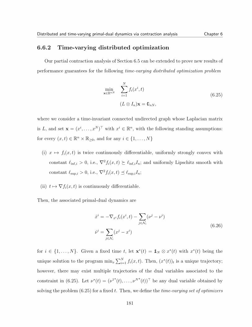
Distributed and time-varying primal-dual dynamics via contraction analysis Chapter 6
6.6.2 Time-varying distributed optimization
Our partial contraction analysis of Section 6.5 can be extended to prove new results of
performance guarantees for the following time-varying distributed optimization problem
minx∈RnN
N∑
i=1
fi(xi, t)
(L⊗ In)x = 0nN ,
(6.25)
where we consider a time-invariant connected undirected graph whose Laplacian matrix
is L, and set x = (xi, . . . , xN)> with xi ∈ Rn, with the following standing assumptions:
for every (x, t) ∈ Rn × R≥0, and for any i ∈ 1, . . . , N
(i) x 7→ fi(x, t) is twice continuously differentiable, uniformly strongly convex with
constant `inf,i > 0, i.e., ∇2fi(x, t) `inf,iIn; and uniformly Lipschitz smooth with
constant `sup,i > 0, i.e., ∇2fi(x, t) `sup,iIn;
(ii) t 7→ ∇fi(x, t) is continuously differentiable.
Then, the associated primal-dual dynamics are
xi = −∇xifi(xi, t)−
∑
j∈Ni
(νj − νi)
νi =∑
j∈Ni
(xj − xi)(6.26)
for i ∈ 1, . . . , N. Given a fixed time t, let x∗(t) = 1N ⊗ x∗(t) with x∗(t) being the
unique solution to the program minx∑N
i=1 fi(x, t). Then, (x∗(t))t is a unique trajectory;
however, there may exist multiple trajectories of the dual variables associated to the
constraint in (6.25). Let ν∗(t) = (ν1∗(t), . . . , νN∗(t))> be any dual variable obtained by
solving the problem (6.25) for a fixed t. Then, we define the time-varying set of optimizers
181

Distributed and time-varying primal-dual dynamics via contraction analysis Chapter 6
as:
M(t) = (x, ν) ∈ RnN × RnN |V (x− 1N ⊗ x∗(t), ν − ν∗(t))> = (0nN , 0n(N−1))>
where V = diag(InN , R ⊗ In) with R ∈ RN−1×N as in the proof of Theorem 6.5.1. For
convenience, let `inf = (`inf,1, . . . , `inf,N) and `sup = (`sup,1, . . . , `sup,N); and for 0 < ε < 1,
we define
αε :=εmini∈1,...,N `inf,i
λ2N + 3
4λNλ2
2 + ‖`sup‖2∞> 0
P :=
InN αε A
∗>
αε A∗ In(N−1)
∈ RnN×nN
(6.27)
where A∗ = (ΛR) ⊗ In, with Λ = diag(λ2, . . . , λN) containing the nonzero eigenvalues
of L in nondecreasing order. The following result establishes the perfomance of the
primal-dual dynamics at tracking the time-varying set of optimizers.
Theorem 6.6.3 [Contraction analysis of time-varying distributed primal-dual
dynamics] Consider the time-varying optimization problem (6.25), its standing assump-
tions, and its associated primal-dual dynamics (6.26). Set z(t) := V (x(t), ν(t))> and
z∗(t) := V (x∗(t), ν∗(t))>.
(i) The system associated to z is contractive with respect to ‖·‖2,P 1/2 with rate c :=
αε34
λ22
λN+1.
Moreover, for any t ≥ 0, if∥∥∥∇fi(x, t)
∥∥∥2≤ β1,i for some positive constant β1,i and any
i ∈ 1, . . . , N, then,
182

Distributed and time-varying primal-dual dynamics via contraction analysis Chapter 6
(ii)
‖z(t)− z∗(t)‖2,P 1/2 ≤(‖z(0)− z∗(0)‖2,P 1/2 − ρ
c
)e−ct +
ρ
c, (6.28)
i.e., the tracking error is asymptotically bounded by ρc
with
ρ = λmax(P )‖β1‖1
‖`inf‖1
N + λmax(P )‖β1‖1
λ2
(‖`sup‖∞‖`inf‖1
+ 1
). (6.29)
Proof: Define f(x(t), t) :=∑N
i=1 fi(xi(t), t); then
z =
−∇f(x(t), t)− (L⊗ In)ν(t)
(ΛR⊗ In)x(t)
.
Then, decomposing (x(t), ν(t))> = U(x(t), ν(t))>+ V >z where U = In(2N−1)− V >V is a
projection matrix, we use the chain rule and obtain that the Jacobian for this system is
−∇2f(x(t), t) −(R>Λ⊗ In)
(ΛR⊗ In) 0n(N−1)×n(N−1)
,
so then, based on our standing assumptions, using Proposition 6.2.1 and following a
similar proof to Theorem 6.5.1, we obtain that this system is contractive as in item (i).
Now we prove statement (ii). The KKT conditions that the optimizers x∗(t) and
ν∗(t) must satisfy (i.e., the equilibrium equation of the system (6.26)), for any t, are
0nN = −∇f(x∗(t), t)− (L⊗ In)ν∗(t) (6.30)
0nN = (L⊗ In)x∗(t). (6.31)
183

Distributed and time-varying primal-dual dynamics via contraction analysis Chapter 6
Now, observe that (6.31) and (6.30) =⇒ x∗(t) = 1N⊗x∗(t) with x∗(t) being the first nN
coordinates of any element ofM(t). Moreover, by left multiplying (6.31) with 1>N⊗In, we
obtain that 0n =∑N
i=1∇xifi(x∗(t), t). Then, the Implicit Function Theorem [2, Theorem
2.5.7] (akin to its use in the proof of Theorem 6.6.1) implies the curve t 7→ x∗(t) is
continuously differentiable for any t ∈ R≥0.
Now, from (6.30) we obtain that 0n(N−1) = (R ⊗ In)∇f(x∗(t), t) + (Λ ⊗ In)(R ⊗
In)ν∗(t). Defining y∗(t) := (R ⊗ In)ν∗(t), we get 0n(N−1) = (R ⊗ In)∇f(x∗(t), t) + (Λ⊗
In)y∗(t). Again, an application of the Implicit Function Theorem let us conclude that
the solution (x∗, t) 7→ y∗(x∗, t) is continuously differentiable for any (x∗, t) ∈ RnN ×R≥0;
however, since t 7→ x∗(t) is continuously differentiable for any t ∈ R≥0, then t 7→ y∗(t) is
continuously differentiable too.
Then, we can differentiate equation (6.30) and left multiply it by (1>N ⊗ In) to obtain
x∗(t) = −(
N∑
i=1
∇2xifi(x
∗(t))
)−1 N∑
i=1
∇xifi(x∗(t), t)).
Recall that RL = ΛR. Then, since y∗ is continuously differentiable, we differentiate
equation (6.30) and left multiply it by (R⊗ In) to obtain
y∗(t) = −(Λ−1R⊗ In)(∇2f(x∗(t), t)(1N ⊗ h1(x∗(t)) + ∇f(x∗(t), t)).
Therefore, observe that∥∥x∗(t)
∥∥2≤ 1∑N
i=1 `inf,i
∑Ni=1 β1,i = ‖β1‖1
‖`inf‖1, and x∗(t) = 1N ⊗ x∗(t).
Moreover,∥∥y∗(t)
∥∥2≤ 1|λ2|
(‖`sup‖∞
∥∥x∗(t)∥∥
2+ ‖β1‖1
), where we used:
∥∥∥∇f(x∗(t), t)∥∥∥
2≤
∑Ni=1
∥∥∥∇xifi(x∗(t))
∥∥∥2, and ‖(Λ−1R)⊗ In‖2 =
√λmax(Λ−2 ⊗ In) = 1
λ2.
Now, for any t, let (a1(t), a2(t)) ∈ M(t). Note that, no matter which element of M
we choose, a1(t) = 1N ⊗ x∗(t) and so it is uniquely defined for any t and we also know
is differentiable. Now, note that a2(t) = γ(t) + 1N ⊗ α, with α ∈ Rn and some uniquely
184

Distributed and time-varying primal-dual dynamics via contraction analysis Chapter 6
defined γ(t); and note that (R⊗In)a2(t) = (R⊗In)γ(t) for any t. Therefore (R⊗In)a2(t) is
uniquely defined for any t and we also know is differentiable. In conclusion, the trajectory
((a1(t), (R⊗ In)a2(t)))t≥0 =(V (a1(t), a2(t))>
)t≥0
is unique and t 7→ V (a1(t), a2(t))> is a
continuously differentiable curve.
Since the system associated to z is contractive and the curve, as we just proved
above, t 7→ z∗(t) := V (x∗(t), ν∗(t))> is unique and differentiable, we set ∆(t) := ‖z(t)−
z∗(t)‖2,P 1/2 and use the result in item (i) and [132, Lemma 2] to obtain the differential
inequality
∆(t) ≤ −c∆(t) +
∥∥∥∥∥∥∥
x∗(t)
ddt
((R⊗ In)ν∗(t))
∥∥∥∥∥∥∥2,P 1/2
≤ −c∆(t) + λmax(P )(N∥∥x∗(t)
∥∥2
+∥∥z∗(t)
∥∥2).
Finally, replacing our previous results and using the Comparison Lemma [94] conclude
the proof for (ii).
Remark 6.6.4 As in Remark 6.6.2, there is consistency on the right-hand side of equa-
tion (6.29).
6.7 Conclusion
Primal-dual (PD) dynamics associated to linear equality constrained optimization
problems are studied in centralized, distributed and time-varying cases. Contraction
theory provides an overarching analysis of the dynamical behavior and performance for
all these cases of PD dynamics. As future work, we plan to design controllers that can
improve the PD solver’s tracking properties in the time-varying setting. We also plan
to study distributed PD solvers for globally coupled linear equation constraints and PD
185

Distributed and time-varying primal-dual dynamics via contraction analysis Chapter 6
solvers in nonsmooth domains.
6.8 Appendix
6.8.1 Proof of Proposition 6.2.1
We remark that the proof of Proposition 6.2.1 is complementary to the one given (for
a slightly different case) in [23, Theorem 3.6]). Proof: Let P :=
−B −A>
A 0m×m
be the matrix in the proposition statement. First, note that <(λ(P )) ≤ µ2(P ) = 0.
Therefore, every eigenvalue of P has non-positive real part. We first show that P has no
eigenvalue equal to zero. Note that by the Schur complement determinant identity, we
have det(P ) = det(−B)) det(−AB−1A>). Note that B b1In, therefore det(−B) 6= 0.
Also, note that B−1 b−12 In; and thus AB−1A> A(b−1
2 In)A> = b−12 AA> 0, where the
last inequality follows from AA> being invertible. This implies that det(−AB−1A>) 6= 0.
As a result, det(P ) 6= 0 and P has no zero eigenvalue. Now we show that P is Hurwitz.
Assume that λ = iη is an eigenvalue of P with zero real part. This means that, there
exists u ∈ Cn and v ∈ Cm such that
−B −A>
A 0m×m
u
v
= iη
u
v
. (6.32)
Multiplying this equation from the left by [uH , vH ], we get
<
[uH vH
]−B −A>
A 0m×m
u
v
= 0.
186

Distributed and time-varying primal-dual dynamics via contraction analysis Chapter 6
This implies that <(uHBu
)= 0. Assume that u = θ1 + iθ2, where θ1, θ2 ∈ Rn. Then
<(uHBu
)= 0 is equivalent to θT1 Bθ1 + θ>2 Bθ2 = 0. Since B b1In, we get that u = 0n.
As a result, the equation (6.32) can be written as the system A>v = 0n and v = 0k. This
implies that if
u
v
∈ Cn+m is an eigenvector associated to the eigenvalue λ = iη, then
u
v
= 0n+m. Thus, the matrix P has no eigenvalue with zero real part. Therefore, the
real part of every eigenvalue of P is negative and the matrix P is Hurwitz.
6.8.2 A simple generalization of [113, Lemma 6]
Lemma 6.8.1 (Convergence of weakly contractive systems) Consider the dynam-
ical system x = f(x, t), x ∈ Rn, where f is continuously-differentiable with respect to x
and weakly contractive respect to some norm ‖·‖, and let x∗ be an equilibrium for the
system, i.e., f(x∗, t) = 0n, for every t ≥ 0. Then x∗ is locally asymptotically stable if
and only if it is globally asymptotically stable.
Proof: We only prove the nontrivial implication: if x∗ is locally asymptotically
stable then it is globally asymptotically stable. Since x∗ is a locally asymptotically
stable equilibrium point for the dynamical system, then there exists ε > 0, such that, for
every y ∈ B(x∗, ε) we have φ(t, 0, y) → x∗ as t → ∞. Note that, for every z ∈ B(x∗, ε),
there exists Tz such that φ(Tz, 0, z) ∈ B(x∗, ε/2). Using the fact that the closed ball
B(x∗, ε) is compact, we get that, there exists T such that, for every z ∈ B(x∗, ε), we
have φ(T, 0, z) ∈ B(x∗, ε/2). Suppose that t 7→ x(t) is a trajectory of the dynamical
system. Assume that y ∈ ∂B(x∗, ε) is a point on the straight line connecting x(0) to
the unique equilibrium point x∗. Then we have ‖x(T )− x∗‖ ≤ ‖x(T )− φ(T, 0, y)‖ +
‖φ(T, 0, y)− x∗‖ ≤ ‖x(0)− y‖ + ε/2 = ‖x(0) − x∗‖ − ε/2. Therefore, after time T ,
187

t 7→ ‖x(t)− x∗‖ decreases by ε/2. As a result, there exists a finite time Tinf such that,
for every t ≥ Tinf , we have x(t) ∈ B(x∗, ε). Since B(x∗, ε) is in the region of attraction of
x∗ the trajectory t 7→ x(t) converges to x∗.
188

Bibliography
[1] R. P. Abelson and J. C. Miller. Negative persuasion via personal insult. Journal ofExperimental Social Psychology, 3(4):321–333, 1967. doi:10.1016/0022-1031(67)90001-7.
[2] R. Abraham, J. E. Marsden, and T. S. Ratiu. Manifolds, Tensor Analysis, andApplications, volume 75 of Applied Mathematical Sciences. Springer, 2 edition,1988.
[3] P.-A. Absil, R. Mahony, and B. Andrews. Convergence of the iterates of descentmethods for analytic cost functions. SIAM Journal on Control and Optimization,6(2):531–547, 2005. doi:10.1137/040605266.
[4] D. Acemoglu, G. Como, F. Fagnani, and A. Ozdaglar. Opinion fluctuations anddisagreement in social networks. Mathematics of Operation Research, 38(1):1–27,2013. doi:10.1287/moor.1120.0570.
[5] D. Acemoglu and A. Ozdaglar. Opinion dynamics and learning in social net-works. Dynamic Games and Applications, 1(1):3–49, 2011. doi:10.1007/
s13235-010-0004-1.
[6] M. Agueh and G. Carlier. Barycenters in the Wasserstein space. SIAM Journal onMathematical Analysis, 43:904–924, 2011. doi:10.1137/100805741.
[7] C. Altafini. Consensus problems on networks with antagonistic interactions. IEEETransactions on Automatic Control, 58(4):935–946, 2013. doi:10.1109/TAC.2012.2224251.
[8] P. C. Alvarez Esteban, E. del Barrio, J. A. Cuesta-Albertos, and C. Matran. Afixed-point approach to barycenters in Wasserstein space. Journal of MathematicalAnalysis and Applications, 441(2):744–762, 2016. doi:10.1016/j.jmaa.2016.04.045.
[9] Z. Aminzare, Y. Shafi, M. Arcak, and E. D. Sontag. Guaranteeing spatial uni-formity in reaction-diffusion systems using weighted L2 norm contractions. In A
189

Systems Theoretic Approach to Systems and Synthetic Biology I: Models and Sys-tem Characterizations, chapter 3, pages 73–101. Springer, 2014. doi:10.1007/
978-94-017-9041-3_3.
[10] Z. Aminzare and E. D. Sontag. Logarithmic Lipschitz norms and diffusion-inducedinstability. Nonlinear Analysis: Theory, Methods & Applications, 83:31–49, 2013.doi:10.1016/j.na.2013.01.001.
[11] Z. Aminzare and E. D. Sontag. Contraction methods for nonlinear systems: A briefintroduction and some open problems. In IEEE Conf. on Decision and Control,pages 3835–3847, December 2014. doi:10.1109/CDC.2014.7039986.
[12] Z. Aminzare and E. D. Sontag. Synchronization of diffusively-connected non-linear systems: Results based on contractions with respect to general norms.IEEE Transactions on Network Science and Engineering, 1(2):91–106, 2014. doi:10.1109/TNSE.2015.2395075.
[13] E. Anderes, S. Borgwardt, and J. Miller. Discrete Wasserstein barycenters: Optimaltransport for discrete data. Mathematical Methods of Operations Research, 85:389–409, 2016. doi:10.1007/s00186-016-0549-x.
[14] T. Antal, P. L. Krapivsky, and S. Redner. Dynamics of social balance on networks.Physical Review E, 72(3):036121, 2005. doi:10.1103/PhysRevE.72.036121.
[15] T. Antal, P. L. Krapivsky, and S. Redner. Social balance on networks: The dynam-ics of friendship and enmity. Physica D: Nonlinear Phenomena, 224(1):130–136,2006. doi:10.1016/j.physd.2006.09.028.
[16] M. Arcak. Certifying spatially uniform behavior in reaction-diffusion PDE andcompartmental ODE systems. Automatica, 47(6):1219–1229, 2011. doi:10.1016/
j.automatica.2011.01.010.
[17] A. Aron and G. Lewandowski. Psychology of interpersonal attraction. In N. J.Smelser and P. B. Baltes, editors, International Encyclopedia of the Social & Behav-ioral Sciences, pages 7860–7862. Pergamon, 2001. doi:10.1016/B0-08-043076-7/01787-3.
[18] K. J. Arrow, L. Hurwicz, and H. Uzawa, editors. Studies in Linear and NonlinearProgramming. Standford University Press, 1958.
[19] F. Battiston, G. Cencetti, I. Iacopini, V. Latora, M. L., A. Patania, J.-G. Young,and G. Petri. Networks beyond pairwise interactions: Structure and dynamics.Physics Reports, 874:1–92, 2020. doi:10.1016/j.physrep.2020.05.004.
[20] M. Baum, P. K. Willett, and U. D. Hanebeck. On Wasserstein barycenters andMMOSPA estimation. IEEE Signal Processing Letters, 22(10):1511–1515, 2015.doi:10.1109/LSP.2015.2410217.
190

[21] J.-D. Benamou and Y. Brenier. A computational fluid mechanics solution to theMonge-Kantorovich mass transfer problem. Numerische Mathematik, 84:375–393,2000. doi:10.1007/s002110050002.
[22] A. R. Benson, R. Abebe, M. T. Schaub, A. Jadbabaie, and J. Kleinberg. Simplicialclosure and higher-order link prediction. Proceedings of the National Academy ofSciences, 115(48):E11221–E11230, 2018. doi:10.1073/pnas.1800683115.
[23] M. Benzi, G. H. Golub, and J. Liesen. Numerical solution of saddle point problems.Acta Numerica, 14:1–137, 2005. doi:10.1017/S0962492904000212.
[24] A. N. Bishop. Information fusion via the Wasserstein barycenter in the space ofprobability measures: Direct fusion of empirical measures and Gaussian fusion withunknown correlation. In International Conference on Information Fusion, pages1–7, 2014.
[25] A. N. Bishop and A. Doucet. Distributed nonlinear consensus in the space ofprobability measures. IFAC Proceedings Volumes, 47(3):8662–8668, 2014. doi:
10.3182/20140824-6-ZA-1003.00341.
[26] F. Blanchini and S. Miani. Set-Theoretic Methods in Control. Springer, 2015.
[27] E. Boissard, T. Le Gouic, and J.-M. Loubes. Distribution’s template estimate withWasserstein, metrics. Bernoulli, 21(2):740–759, 2015. doi:10.3150/13-BEJ585.
[28] P. Bonacich, A. C. Holdren, and M. Johnston. Hyper-edges and multidimensionalcentrality. Social Networks, 26(3):189–203, 2004. doi:10.1016/j.socnet.2004.
01.001.
[29] N. Bonneel, G. Peyre, and M. Cuturi. Wasserstein barycentric coordinates: His-togram regression using optimal transport. ACM Transactions on Graphics, 35(4),2016. doi:10.1145/2897824.2925918.
[30] N. Bonneel, J. Rabin, G. Peyre, and H. Pfister. Sliced and radon Wassersteinbarycenters of measures. Journal of Mathematical Imaging and Vision, 51(1):22–45, 2015. doi:10.1007/s10851-014-0506-3.
[31] S. Boyd, A. Ghosh, B. Prabhakar, and D. Shah. Randomized gossip algorithms.IEEE Transactions on Information Theory, 52(6):2508–2530, 2006. doi:10.1109/TIT.2006.874516.
[32] F. Bullo. Lectures on Network Systems. Kindle Direct Publishing, 1.3 edition,July 2019. With contributions by J. Cortes, F. Dorfler, and S. Martınez. URL:http://motion.me.ucsb.edu/book-lns.
191

[33] F. Bullo. Lectures on Network Systems. Kindle Direct Publishing, 1.4 edition,July 2020. With contributions by J. Cortes, F. Dorfler, and S. Martınez. URL:http://motion.me.ucsb.edu/book-lns.
[34] G. Buttazzo, L. De Pascale, and P. Gori-Giorgi. Optimal-transport formulation ofelectronic density-functional theory. Physical Review A, 85, 2012. doi:10.1103/
PhysRevA.85.062502.
[35] S. Byrne and P. Solomon Hart. The boomerang effect. A synthesis of findings anda preliminary theoretical framework. Annals of the International CommunicationAssociation, 33(1):3–37, 2009. doi:10.1080/23808985.2009.11679083.
[36] G. Carlier and I. Ekeland. Matching for teams. Economic Theory, 42:397–418,2010. doi:10.1007/s00199-008-0415-z.
[37] G. Carlier, A. Oberman, and E. Oudet. Numerical methods for matching forteams and Wasserstein barycenters. ESAIM: Mathematical Modelling and Numer-ical Analysis, 49:1621–1642, 2015. doi:10.1051/m2an/2015033.
[38] D. Cartwright and F. Harary. Structural balance: A generalization of Heider’stheory. Psychological Review, 63(5):277, 1956. doi:10.1037/h0046049.
[39] G. Chen, W. Su, W. Mei, and F. Bullo. Convergence properties of the heteroge-neous Deffuant-Weisbuch model. Automatica, 114:108825, 2020. doi:10.1016/j.
automatica.2020.108825.
[40] X. Chen and N. Li. Exponential stability of primal-dual gradient dynamics withnon-strong convexity. In American Control Conference, pages 1612–1618, 2020.doi:10.23919/ACC45564.2020.9147393.
[41] Y. Chen, T. T. Georgiou, and A. Tannenbaum. Optimal transport for Gaussianmixture models. IEEE Access, 7:6269–6278, 2019. doi:10.1109/ACCESS.2018.
2889838.
[42] A. Cherukuri, B. Gharesifard, and J. Cortes. Saddle-point dynamics: Conditions forasymptotic stability of saddle points. SIAM Journal on Control and Optimization,55(1):486–511, 2017. doi:10.1137/15M1026924.
[43] P. Cisneros-Velarde and F. Bullo. Signed network formation games and clus-tering balance. Dynamic Games and Applications, 2020. doi:10.1007/
s13235-019-00346-8.
[44] P. Cisneros-Velarde, S. Jafarpour, and F. Bullo. Distributed and time-varyingprimal-dual dynamics via contraction analysis. IEEE Transactions on AutomaticControl, March 2020. Submitted. URL: https://arxiv.org/pdf/2003.12665.
192

[45] S. Claici, E. Chien, and J. Solomon. Stochastic Wasserstein barycenters. In Inter-national Conference on Machine Learning, volume 80, pages 999–1008, 2018.
[46] A. R. Cohen. A dissonance analysis of the boomerang effect. Journal of Personality,30(1):75–88, 1962. doi:10.1111/j.1467-6494.1962.tb02306.x.
[47] S. Coogan. A contractive approach to separable Lyapunov functions for monotonesystems. Automatica, 106:349–357, 2019. doi:10.1016/j.automatica.2019.05.
001.
[48] W. A. Coppel. Stability and Asymptotic Behavior Of Differential Equations. Heath,1965.
[49] J. Cortes and S. K. Niederlander. Distributed coordination for nonsmooth convexoptimization via saddle-point dynamics. Journal of Nonlinear Science, 29(4):1247–1272, 2019. doi:10.1007/s00332-018-9516-4.
[50] N. Courty, R. Flamary, D. Tuia, and A. Rakotomamonjy. Optimal transport fordomain adaptation. IEEE Transactions on Pattern Analysis and Machine Intelli-gence, 39(9):1853–1865, 2016. doi:10.1109/TPAMI.2016.2615921.
[51] M. Cuturi and A. Doucet. Fast computation of Wasserstein barycenters. In Inter-national Conference on Machine Learning, volume 32, pages 685–693, 2014.
[52] M. Cuturi and G. Peyr. A smoothed dual approach for variational Wassersteinproblems. SIAM Journal on Imaging Sciences, 9:320–343, 2016. doi:doi.org/10.1137/15M1032600.
[53] J. L. Daleckii and M. G. Krein. Stability of Solutions of Differential Equations inBanach Space. American Mathematical Society, 2002.
[54] J. A. Davis. Clustering and structural balance in graphs. Human Relations,20(2):181–187, 1967. doi:10.1177/001872676702000206.
[55] G. F. de Arruda, G. Petri, and Y. Moreno. Social contagion models on hypergraphs.Physical Review Research, 2, 2020. doi:10.1103/PhysRevResearch.2.023032.
[56] G. Deffuant, D. Neau, F. Amblard, and G. Weisbuch. Mixing beliefs amonginteracting agents. Advances in Complex Systems, 3(1/4):87–98, 2000. doi:
10.1142/S0219525900000078.
[57] K. Deimling. Nonlinear Functional Analysis. Springer, 1985.
[58] P. DeLellis, M. Di Bernardo, and G. Russo. On QUAD, Lipschitz, and contractingvector fields for consensus and synchronization of networks. IEEE Transactions onCircuits and Systems I: Regular Papers, 58(3):576–583, 2011. doi:10.1109/TCSI.2010.2072270.
193

[59] M. Di Bernardo, D. Fiore, G. Russo, and F. Scafuti. Convergence, consen-sus and synchronization of complex networks via contraction theory. In J. Lu,X. Yu, G. Chen, and W. Yu, editors, Complex Systems and Networks: Dynam-ics, Controls and Applications, pages 313–339. Springer, 2016. doi:10.1007/
978-3-662-47824-0_12.
[60] A. d’Onofrio. A note on the global behaviour of the network-based SIS epidemicmodel. Nonlinear Analysis: Real World Applications, 9(4):1567–1572, 2008. doi:
10.1016/j.nonrwa.2007.04.001.
[61] P. Dvurechenskii, D. Dvinskikh, A. Gasnikov, C. Uribe, and A. Nedich. Decentralizeand randomize: Faster algorithm for Wasserstein barycenters. In Advances inNeural Information Processing Systems, pages 10760–10770. 2018.
[62] D. Easley and J. Kleinberg. Networks, Crowds, and Markets: Reasoning About aHighly Connected World. Cambridge University Press, 2010.
[63] G. Facchetti, G. Iacono, and C. Altafini. Computing global structural balance inlarge-scale signed social networks. Proceedings of the National Academy of Sciences,108(52):20953–20958, 2011. doi:10.1073/pnas.1109521108.
[64] A. Fall, A. Iggidr, G. Sallet, and J.-J. Tewa. Epidemiological models and Lyapunovfunctions. Mathematical Modelling of Natural Phenomena, 2(1):62–68, 2007. doi:10.1051/mmnp:2008011.
[65] M. Fazlyab, S. Paternain, V. M. Preciado, and A. Ribeiro. Prediction-correctioninterior-point method for time-varying convex optimization. IEEE Transactions onAutomatic Control, 63(7):1973–1986, 2018. doi:10.1109/TAC.2017.2760256.
[66] D. Feijer and F. Paganini. Stability of primal–dual gradient dynamics and ap-plications to network optimization. Automatica, 46(12):1974–1981, 2010. doi:
10.1016/j.automatica.2010.08.011.
[67] L. Festinger. A Theory of Cognitive Dissonance. Stanford University Press, 1957.
[68] S. Fiske and S. E. Taylor. Social Cognition: From Brains to Culture. Sage, 3edition, 2003.
[69] N. E. Friedkin. A Structural Theory of Social Influence. Cambridge UniversityPress, 1998.
[70] N. E. Friedkin, A. V. Proskurnikov, and F. Bullo. Positive contagion and themacrostructures of generalized balance. Network Science, 7(4):445–458, 2019. doi:10.1017/nws.2019.19.
194

[71] D. Gallaun, C. Seifert, and M. Tautenhahn. Sufficient criteria and sharp geomet-ric conditions for observability in Banach spaces. SIAM Journal on Control andOptimization, 58(4):26392657, 2020. doi:10.1137/19M1266769.
[72] S. Galln, J.-M. Loubes, and E. Maza. Statistical properties of the quantile normal-ization method for density curve alignment. Mathematical Biosciences, 242(2):129–142, 2013. doi:10.1016/j.mbs.2012.12.007.
[73] M. Granovetter. Threshold models of collective behavior. The Americal Journalof Sociology, 83(6):1420–1443, 1978. doi:10.1086/226707.
[74] F. Harary. On the notion of balance of a signed graph. Michigan MathematicalJournal, 2(2):143–146, 1953. doi:10.1307/mmj/1028989917.
[75] A. Hatcher. Algebraic Topology. Cambridge University Press, 2002.
[76] F. Heider. Attitudes and cognitive organization. The Journal of Psychology,21(1):107–112, 1946. doi:10.1080/00223980.1946.9917275.
[77] U. Helmke and J. B. Moore. Optimization and Dynamical Systems. Springer, 2edition, 1996.
[78] J. M. Hendrickx. A lifting approach to models of opinion dynamics with antago-nisms. In IEEE Conf. on Decision and Control, pages 2118–2123, December 2014.doi:10.1109/CDC.2014.7039711.
[79] A. Henrot. Extremum Problems for Eigenvalues of Elliptic Operators. Springer,2006.
[80] H. W. Hethcote. An immunization model for a heterogeneous population. The-oretical Population Biology, 14(3):338–349, 1978. doi:10.1016/0040-5809(78)
90011-4.
[81] H. W. Hethcote. The mathematics of infectious diseases. SIAM Review, 42(4):599–653, 2000. doi:10.1137/S0036144500371907.
[82] R. A. Horn and C. R. Johnson. Matrix Analysis. Cambridge University Press, 2ndedition, 2012.
[83] A. R. Hota and S. Sundaram. Game-theoretic vaccination against networked SISepidemics and impacts of human decision-making. IEEE Transactions on Controlof Network Systems, 6(4):1461–1472, 2019. doi:10.1109/TCNS.2019.2897904.
[84] C. I. Hovland, O. J. Harvey, and M. Sherif. Assimilation and contrast effects inreactions to communication and attitude change. The Journal of Abnormal andSocial Psychology, 55(2):244–252, 1957. doi:10.1037/h0048480.
195

[85] T. Hsing and R. Eubank. Theoretical Foundations of Functional Data Analysis,with an Introduction to Linear Operators. John Wiley & Sons, 2015.
[86] H. Huang, J. Tang, L. Liu, J. Luo, and X. Fu. Triadic closure pattern analysisand prediction in social networks. IEEE Transactions on Knowledge and DataEngineering, 27(12):3374–3389, 2015. doi:10.1109/TKDE.2015.2453956.
[87] I. Iacopini, G. Petri, A. Barrat, and V. Latora. Simplicial models of so-cial contagion. Nature Communications, 10(1):2485, 2019. doi:10.1038/
s41467-019-10431-6.
[88] M. O. Jackson and S. Nei. Networks of military alliances, wars, and internationaltrade. Proceedings of the National Academy of Sciences, 112(50):15277–15284, 2015.doi:10.1073/pnas.1520970112.
[89] S. Jafarpour, P. Cisneros-Velarde, and F. Bullo. Weak and semi-contraction for net-work systems and diffusively-coupled oscillators. IEEE Transactions on AutomaticControl, May 2020. Submitted. URL: http://arxiv.org/pdf/2005.09774.
[90] I. M. James and N. J. Hitchin. The Topology of Stiefel Manifolds. CambridgeUniversity Press, 1976.
[91] B. Jhun, M. Jo, and B. Kahng. Simplicial SIS model in scale-free uniformhypergraph. Journal of Statistical Mechanics: Theory and Experiment, 2019.doi:10.1088/1742-5468/ab5367.
[92] P. Jia, N. E. Friedkin, and F. Bullo. The coevolution of appraisal and influencenetworks leads to structural balance. IEEE Transactions on Network Science andEngineering, 3(4):286–298, 2016. doi:10.1109/TNSE.2016.2600058.
[93] K. F. Kee, L. Sparks, D. C. Struppa, and M. Mannucci. Social groups, social media,and higher dimensional social structures: A simplicial model of social aggregationfor computational communication research. Communication Quarterly, 61(1):35–58, 2013. doi:10.1080/01463373.2012.719566.
[94] H. K. Khalil. Nonlinear Systems. Prentice Hall, 3 edition, 2002.
[95] A. Khanafer, T. Basar, and B. Gharesifard. Stability of epidemic models overdirected graphs: A positive systems approach. Automatica, 74:126–134, 2016. doi:10.1016/j.automatica.2016.07.037.
[96] S. S. Kia, J. Cortes, and S. Martinez. Distributed convex optimization viacontinuous-time coordination algorithms with discrete-time communication. Auto-matica, 55:254–264, 2015. doi:10.1016/j.automatica.2015.03.001.
196

[97] K. Ku lakowski, P. Gawronski, and P. Gronek. The Heider balance: A continuousapproach. International Journal of Modern Physics C, 16(05):707–716, 2005. doi:10.1142/S012918310500742X.
[98] M. Kurula. Well-posedness of time-varying linear systems. IEEE Transactions onAutomatic Control, 2019. doi:10.1109/TAC.2019.2954794.
[99] G. E. Ladas and V. Lakshmikantham. Differential Equations in Abstract Spaces.Academic Press, 1972.
[100] A. Lajmanovich and J. A. Yorke. A deterministic model for gonorrhea in anonhomogeneous population. Mathematical Biosciences, 28(3):221–236, 1976.doi:10.1016/0025-5564(76)90125-5.
[101] T. Le Gouic and J.-M. Loubes. Existence and consistency of Wasserstein barycen-ters. Probability Theory and Related Fields, 168:901–917, 2017. doi:10.1007/
s00440-016-0727-z.
[102] J. M. Lee. Introduction to Smooth Manifolds. Springer, 2003.
[103] J. Leskovec, D. Huttenlocher, and J. Kleinberg. Signed networks in social media.In Int. Conf. on Human Factors in Computing Systems, pages 1361–1370, Atlanta,USA, 2010. doi:10.1145/1753326.1753532.
[104] Y. Li, W. Chen, Y. Wang, and Z.-L. Zhang. Voter model on signed social networks.Internet Mathematics, 11(2):93–133, 2015. doi:10.1080/15427951.2013.862884.
[105] S. Liang, L. Y. Wang, and G. Yin. Exponential convergence of distributed primal-dual convex optimization algorithm without strong convexity. Automatica, 105:298–306, 2019. doi:10.1016/j.automatica.2019.04.004.
[106] C.-C. Lin, C.-H. Lee, C.-S. Fuh, H.-F. Juan, and H.-C. Huang. Link clusteringreveals structural characteristics and biological contexts in signed molecular net-works. PLoS One, 8(6):1–9, 06 2013. doi:10.1371/journal.pone.0067089.
[107] X. Lin, Q. Jiao, and L. Wang. Opinion propagation over signed networks: Modelsand convergence analysis. IEEE Transactions on Automatic Control, 64(8):3431–3438, 2019. doi:10.1109/TAC.2018.2879568.
[108] J. Liu, X. Chen, T. Basar, and M.-A. Belabbas. Exponential convergence of thediscrete- and continuous-time Altafini models. IEEE Transactions on AutomaticControl, 62:6168–6182, 2017. doi:10.1109/TAC.2017.2700523.
[109] W.-M. Liu, H. W. Hethcote, and S. A. Levin. Dynamical behavior of epidemio-logical models with nonlinear incidence rates. Journal of Mathematical Biology,25(4):359–380, 1987. doi:10.1007/BF00277162.
197

[110] Y. Liu, C. Lageman, B. D.O. Anderson, and G. Shi. An Arrow-Hurwicz-Uzawa typeflow as least squares solver for network linear equations. Automatica, 100:187–193,2019. doi:10.1016/j.automatica.2018.10.007.
[111] Y. Liu, Y. Lou, B. D. O. Anderson, and G. Shi. Network flows that solve leastsquares for linear equations, 2018. arXiv:1808.04140.
[112] W. Lohmiller and J.-J. E. Slotine. On contraction analysis for non-linear systems.Automatica, 34(6):683–696, 1998. doi:10.1016/S0005-1098(98)00019-3.
[113] E. Lovisari, G. Como, and K. Savla. Stability of monotone dynamical flow networks.In IEEE Conf. on Decision and Control, pages 2384–2389, Los Angeles, USA,December 2014. doi:10.1109/CDC.2014.7039752.
[114] D. G. Luenberger. Optimization by Vector Space Methods. John Wiley & Sons,1969.
[115] M. Malekzadeh, M. Fazli, P. Jalaly Khalidabadi, H. R. Rabiee, and M. A. Safari.Social balance and signed network formation games. In Proceedings of 5th KDDWorkshop on Social Network Analysis (SNA-KDD), San Diego, USA, August 2011.
[116] E. Mallada, C. Zhao, and S. Low. Optimal load-side control for frequency regulationin smart grids. IEEE Transactions on Automatic Control, 62(12):6294–6309, 2017.doi:10.1109/TAC.2017.2713529.
[117] I. R. Manchester and J.-J. E. Slotine. Control contraction metrics: Convex andintrinsic criteria for nonlinear feedback design. IEEE Transactions on AutomaticControl, 62(6):3046–3053, 2017. doi:10.1109/TAC.2017.2668380.
[118] M. Martcheva. An Introduction to Mathematical Epidemiology. Springer, 2015.
[119] S. A. Marvel, J. Kleinberg, R. D. Kleinberg, and S. H. Strogatz. Continuous-timemodel of structural balance. Proceedings of the National Academy of Sciences,108(5):1771–1776, 2011. doi:10.1073/pnas.1013213108.
[120] S. A. Marvel, S. H. Strogatz, and J. M. Kleinberg. Energy landscape of socialbalance. Physical Review Letters, 103:198701, 2009. doi:10.1103/PhysRevLett.
103.198701.
[121] J. T. Matamalas, S. Gomez, and A. Arenas. Abrupt phase transition of epidemicspreading in simplicial complexes. Physical Review Research, 2:012049, 2020. doi:10.1103/PhysRevResearch.2.012049.
[122] W. Mei, P. Cisneros-Velarde, G. Chen, N. E. Friedkin, and F. Bullo. Dynamicsocial balance and convergent appraisals via homophily and influence mechanisms.Automatica, 110:108580, 2019. doi:10.1016/j.automatica.2019.108580.
198

[123] W. Mei, S. Mohagheghi, S. Zampieri, and F. Bullo. On the dynamics of determin-istic epidemic propagation over networks. Annual Reviews in Control, 44:116–128,2017. doi:10.1016/j.arcontrol.2017.09.002.
[124] Ziyang Meng, Guodong Shi, Karl H. Johansson, Ming Cao, and Yiguang Hong.Behaviors of networks with antagonistic interactions and switching topologies. Au-tomatica, 73:110 – 116, 2016. doi:https://doi.org/10.1016/j.automatica.
2016.06.022.
[125] A. N. Michel, L. Hou, and D. Liu. Stability of Dynamical Systems. Springer, 2008.
[126] A. Mironchenko and F. Wirth. Characterizations of input-to-state stabilityfor infinite-dimensional systems. IEEE Transactions on Automatic Control,63(6):1692–1707, 2018. doi:10.1109/TAC.2017.2756341.
[127] Y. Mroueh. Wasserstein style transfer. In International Conference on ArtificialIntelligence and Statistics, volume 108, pages 842–852, 2020.
[128] J. Munkres. Topology. Pearson, 2 edition, 2000.
[129] J. D. Murray. Mathematical Biology I: An Introduction. Springer, 3 edition, 2002.
[130] J. Muscat. Functional Analysis: An Introduction to Metric Spaces, Hilbert Spaces,and Banach Algebras. Springer, 2014.
[131] P. H. A. Ngoc and H. Trinh. On contraction of functional differential equations.SIAM Journal on Control and Optimization, 56(3):2377–2397, 2018. doi:10.1137/16M1092672.
[132] H. D. Nguyen, T. L. Vu, K. Turitsyn, and J.-J. E. Slotine. Contraction and ro-bustness of continuous time primal-dual dynamics. IEEE Control Systems Letters,2(4):755–760, 2018. doi:10.1109/LCSYS.2018.2847408.
[133] C. Nowzari, V. M. Preciado, and G. J. Pappas. Analysis and control of epidemics:A survey of spreading processes on complex networks. IEEE Control Systems,36(1):26–46, 2016. doi:10.1109/MCS.2015.2495000.
[134] P. J. Oakes and J. C. Turner. Is limited information processing capacity the causeof social stereotyping? European Review of Social Psychology, 1(1):111–135, 1990.doi:10.1080/14792779108401859.
[135] M. Ogura, V. M. Preciado, and N. Masuda. Optimal containment of epidemicsover temporal activity-driven networks. SIAM Journal on Applied Mathematics,79(3), 2019. doi:10.1137/18M1172740.
199

[136] K. Paarporn, C. Eksin, J. S. Weitz, and J. S. Shamma. Networked SIS epidemicswith awareness. IEEE Transactions on Computational Social Systems, 4(3):93–103,2017. doi:10.1109/TCSS.2017.2719585.
[137] V. M. Panaretos and Y. Zemel. An Invitation to Statistics in Wasserstein Space.SpringerBriefs in Probability and Mathematical Statistics. Springer, 2020. doi:
10.1007/978-3-030-38438-8.
[138] P. E. Pare, C. L. Beck, and A. Nedic. Epidemic processes over time-varying net-works. IEEE Transactions on Control of Network Systems, 5(3), 2017. doi:
10.1109/TCNS.2017.2706138.
[139] P. E. Pare, J. Liu, C. L. Beck, A. Nedic, and T. Basar. Multi-competitive virusesover static and time-varying networks. In American Control Conference, pages1685–1690, 2017. doi:10.23919/ACC.2017.7963195.
[140] R. Pastor-Satorras and A. Vespignani. Epidemic spreading in scale-free networks.Physical Review Letters, 86(14):3200–3203, 2001. doi:10.1103/PhysRevLett.86.3200.
[141] A. Pavlov, A. Pogromsky, N. Van de Wouw, and H. Nijmeijer. Convergent dy-namics, a tribute to Boris Pavlovich Demidovich. Systems & Control Letters, 52(3-4):257–261, 2004. doi:10.1016/j.sysconle.2004.02.003.
[142] Q. C. Pham and J.-J. E. Slotine. Stable concurrent synchronization in dynamicsystem networks. Neural Networks, 20(1):62–77, 2007. doi:10.1016/j.neunet.
2006.07.008.
[143] A. Polyakov, J. Coron, and L. Rosier. On homogeneous finite-time control for linearevolution equation in Hilbert space. IEEE Transactions on Automatic Control,63(9):3143–3150, 2018. doi:10.1109/TAC.2018.2797838.
[144] A. V. Proskurnikov and R. Tempo. A tutorial on modeling and analysis of dynamicsocial networks. Part I. Annual Reviews in Control, 43:65–79, 2017. doi:10.1016/j.arcontrol.2017.03.002.
[145] G. Qu and N. Li. On the exponential stability of primal-dual gradient dynam-ics. IEEE Control Systems Letters, 3(1):43–48, 2019. doi:10.1109/LCSYS.2018.
2851375.
[146] J. Rabin, G. Peyre, J. Delon, and M. Bernot. Wasserstein barycenter and itsapplication to texture mixing. In Scale Space and Variational Methods in ComputerVision, pages 435–446. Springer, 2012. doi:10.1007/978-3-642-24785-9_37.
[147] F. Radicchi, D. Vilone, S. Yoon, and H. Meyer-Ortmanns. Social balance as asatisfiability problem of computer science. Physical Review E, 75:026106, 2007.doi:10.1103/PhysRevE.75.026106.
200

[148] S. Rahili and W. Ren. Distributed continuous-time convex optimization with time-varying cost functions. IEEE Transactions on Automatic Control, 62(4):1590–1605,2017. doi:10.1109/TAC.2016.2593899.
[149] R. T. Rockafellar. Augmented Lagrangians and applications of the proximal pointalgorithm in convex programming. Mathematics of Operations Research, 1(2):97–116, 1976. doi:10.1287/moor.1.2.97.
[150] F. D. Sahneh, C. Scoglio, and P. Van Mieghem. Generalized epidemic mean-field model for spreading processes over multilayer complex networks. IEEE/ACMTransactions on Networking, 21(5):1609–1620, 2013. doi:10.1109/TNET.2013.
2239658.
[151] F. Santambrogio. Optimal Transport for Applied Mathematicians: Calculus ofVariations, PDEs, and Modeling. Progress in Nonlinear Differential Equationsand Their Applications. Birkhauser, 2015. doi:10.1007/978-3-319-20828-2.
[152] M. T. Schaub, A. R. Benson, P. Horn, G. Lippner, and A. Jadbabaie. Random walkson simplicial complexes and the normalized Hodge 1-Laplacian. SIAM Review,62(2):353–391, 2020. doi:10.1137/18M1201019.
[153] M. A. Schmitz, M. Heitz, N. Bonneel, F. Ngole, D. Coeurjolly, M. Cuturi, G. Peyre,and J.-L. Starck. Wasserstein dictionary learning: Optimal transport-based unsu-pervised nonlinear dictionary learning. SIAM Journal on Imaging Sciences, 11:643–678, 2018. doi:10.1137/17M1140431.
[154] V. Seguy and M. Cuturi. Principal geodesic analysis for probability measuresunder the optimal transport metric. In Advances in Neural Information ProcessingSystems, pages 3312–3320. 2015.
[155] J. H. Shapiro. A Fixed-Point Farrago. Springer, 2016.
[156] G. Shi, C. Altafini, and J. Baras. Dynamics over signed networks. SIAM Review,61(2):229–257, 2019. doi:10.1137/17M1134172.
[157] J. W. Simpson-Porco and F. Bullo. Contraction theory on Riemannian manifolds.Systems & Control Letters, 65:74–80, 2014. doi:10.1016/j.sysconle.2013.12.
016.
[158] J. W. Simpson-Porco, B. K. Poolla, N. Monshizadeh, and F. Dorfler. Input-outputperformance of linear-quadratic saddle-point algorithms with application to dis-tributed resource allocation problems. IEEE Transactions on Automatic Control,65(5):2032–2045, 2019. doi:10.1109/TAC.2019.2927328.
[159] S. Srivastava, V. Cevher, Q. Dinh, and D. Dunson. WASP: scalable Bayes viabarycenters of subset posteriors. In International Conference on Artificial Intelli-gence and Statistics, volume 38, pages 912–920, 2015.
201

[160] C. Sun, M. Ye, and G. Hu. Distributed time-varying quadratic optimization formultiple agents under undirected graphs. IEEE Transactions on Automatic Con-trol, 62(7):3687–3694, 2017. doi:10.1109/TAC.2017.2673240.
[161] A. Tahbaz-Salehi and A. Jadbabaie. Consensus over ergodic stationary graphprocesses. IEEE Transactions on Automatic Control, 55(1):225–230, 2010. doi:
10.1109/TAC.2009.2034054.
[162] R. Tempo, G. Calafiore, and F. Dabbene. Randomized Algorithms for Analysis andControl of Uncertain Systems. Springer, 2005.
[163] A. Terrand-Jeanne, V. Andrieu, V. Dos Santos Martins, and C. Xu. Adding integralaction for open-loop exponentially stable semigroups and application to boundarycontrol of PDE systems. IEEE Transactions on Automatic Control, 2019. doi:
10.1109/TAC.2019.2957349.
[164] V. A. Traag, P. Van Dooren, and P. De Leenheer. Dynamical models explainingsocial balance and evolution of cooperation. PLoS One, 8(4):e60063, 2013. doi:
10.1371/journal.pone.0060063.
[165] E. Trlat, C. Zhang, and E. Zuazua. Steady-state and periodic exponential turnpikeproperty for optimal control problems in Hilbert spaces. SIAM Journal on Controland Optimization, 56(2):12221252, 2018. doi:10.1137/16M1097638.
[166] C. A. Uribe, D. Dvinskikh, P. Dvurechensky, A. Gasnikov, and A. Nedi. Distributedcomputation of Wasserstein barycenters over networks. In IEEE Conf. on Decisionand Control, pages 6544–6549, 2018. doi:10.1109/CDC.2018.8619160.
[167] A. van de Rijt. The micro-macro link for the theory of structural balance. Journalof Mathematical Sociology, 35(1-3):94–113, 2011. doi:10.1080/0022250X.2010.
532262.
[168] M. Vidyasagar. Nonlinear Systems Analysis. SIAM, 2002. doi:10.1137/1.
9780898719185.
[169] C. Villani. Topics in Optimal Transportation. Graduate Studies in Mathematics.American Mathematical Society, 2003.
[170] C. Villani. Optimal Transport: Old and New. Springer, 2009. doi:10.1007/
978-3-540-71050-9.
[171] M. Wakaiki and H. Sano. Event-triggered control of infinite-dimensional systems.SIAM Journal on Control and Optimization, 58(2):605–635, 2020. doi:10.1137/
18M1179717.
[172] G. Wang, Y. Wei, and S. Qiao. Generalized Inverses: Theory and Computations.Springer, 2018.
202

[173] J. Wang and N. Elia. A control perspective for centralized and distributed convexoptimization. In IEEE Conf. on Decision and Control and European Control Con-ference, pages 3800–3805, Orlando, USA, 2011. doi:10.1109/CDC.2011.6161503.
[174] P. Wang, S. Mou, J. Lian, and W. Ren. Solving a system of linear equations: Fromcentralized to distributed algorithms. Annual Reviews in Control, 47:306–322, 2019.doi:10.1016/j.arcontrol.2019.04.008.
[175] N. J. Watkins, C. Nowzari, and G. J. Pappas. Robust economic model predictivecontrol of continuous-time epidemic processes. IEEE Transactions on AutomaticControl, 65(3):1116–1131, 2020. doi:10.1109/TAC.2019.2919136.
[176] T. Yang, X. Yi, J. Wu, Y. Yuan, D. Wu, Z. Meng, Y. Hong, H. Wang, Z. Lin, andK. H. Johansson. A survey of distributed optimization. Annual Reviews in Control,47:278–305, 2019. doi:10.1016/j.arcontrol.2019.05.006.
[177] X. Zheng, D. Zeng, and F.-Y. Wang. Social balance in signed networks. InformationSystems Frontiers, 17(5):1077–1095, 2015. doi:10.1007/s10796-014-9483-8.
203