Journal of High Speed Networks 16 (2007) 353–377 353IOS Press

Network profit optimization for trafficgrooming in WDM networkswith wavelength converters

James Yiming Zhang a, Jing Wu b,∗, Oliver Yang a and Michel Savoie b

a School of Information Technology and Engineering, University of Ottawa, Ottawa, ON, K1N 6N5, CanadaE-mail: {yizhang, yang}@site.uottawa.cab Communications Research Centre Canada, Ottawa, ON, K2H 8S2, CanadaE-mail: {jing.wu, michel.savoie}@crc.ca

Abstract. The traffic grooming technique provides a two-layer traffic engineering capability by aggregating and routing up-layer low-bandwidthtraffic flows over low-layer re-configurable routed high-bandwidth connections. In this paper, we optimize traffic grooming for static traffic inmesh Wavelength Division Multiplexing (WDM) networks with wavelength converters. The optimization objective is to maximize networkprofit, which is the difference between resource cost and the revenue generated (by selecting profitable traffic flows). A constrained integerlinear programming formulation is given, and a decomposition using Lagrangian relaxation is proposed. We then present a systematic approachto solve this problem and to obtain a performance bound for an arbitrary topology mesh network. Our approach can select traffic flows based ontheir profit, while obtaining their data path routing, lightpath routing and wavelength assignment at the same time. Our performance evaluationalso reveals the impact of various cost parameters on the profit objective.

Keywords: WDM networks, traffic grooming, routing and wavelength assignment, network profit optimization, Lagrangian relaxation,wavelength conversion

1. Introduction

Wavelength routing in Wavelength Division Multiplexing (WDM) networks enables the re-configuration of vir-tual topologies of optical networks, and provides an opportunity for joint two-layer traffic engineering [1–4].Lightpaths are routed in a WDM network and each of them is assigned to a wavelength channel on a link. Sincewavelength converters may be used, a lightpath may use different wavelengths on different links. At the entry ofa lightpath, electrical domain traffic flows are aggregated (i.e., groomed) together and carried by the lightpath.In this paper, we simply refer to the electrical domain traffic flows as traffic flows. At the intermediate nodes of alightpath, the traffic flows pass through optical switches without electrical processing. At the exit of a lightpath, theindividual traffic flows are restored to their electrical form. If a traffic flow has not yet reached its final destination,it is groomed with other traffic flows and carried by another lightpath. We refer the traffic grooming type discussedherein as multi-hop traffic grooming [5], where the lightpath bandwidth is shared by traffic flows between differentsource-destination pairs. The multi-hop traffic grooming problem is an extension of the virtual topology designproblem of a WDM network. It is a joint design issue of two layers of traffic engineering: the routing of lightpathsover fibres, and the routing of traffic flows over lightpaths. This traffic grooming problem and the associated cross-layer cost minimization aspects have not been addressed in most of the virtual topology design studies (e.g., seesurvey [2]).

*Corresponding author: Jing Wu, Communications Research Centre Canada, Ottawa, ON, K2H 8S2, Canada. Tel.: +1 613 998 2474; Fax:+1 613 990-8382; E-mail: jing.wu@crc.ca.

0926-6801/07/$17.00 © 2007 – IOS Press and the authors. All rights reserved

354 J.Y. Zhang et al. / Network profit optimization in WDM networks

Traffic grooming research has two flavours: static and dynamic. Depending on whether the arrival and departuretime of traffic flows are random or are known in advance, traffic grooming is classified as dynamic (e.g., [5,10])and static (e.g., [6–9]), respectively. In this paper, we study the static traffic grooming.

For the static traffic grooming problem, how to select profitable traffic flows is an untouched problem. Assumingthat all the traffic flows should be accepted, most previous studies aim at minimizing costs [2,9,17]. This assump-tion is not practical: the revenue generated by some traffic flows may not recover their provisioning costs, becauseno efficient provisioning scheme exists for them. A few previous studies dealt with the throughput maximizationor revenue optimization problems [8,18,19], by using throughput maximization to prioritize the traffic flows basedon their efficiency of resource utilization. Unfortunately, the efficiency of traffic grooming and lightpath provi-sioning schemes is implicitly evaluated without modelling the cost. Therefore, it is unknown whether providingservice to a traffic flow is profitable or not. The revenue optimization is a variation of throughput maximization.For a given network, the revenue maximization leads to maximal profit. The revenue was modelled as a weightedthroughput [8] or modelled based on service differentiation for lightpath protection [18], but the cost parameterswere not modelled, and their impact on the profit was not studied. While maximizing throughput and minimizingthe number of lightpaths were modelled in [19] as two competing objectives and were jointly optimized using themulti-objective optimization technique, the relationship of these two objectives to the profit was not revealed. Inthis paper, we study the static traffic grooming in WDM networks with wavelength converters. Different from theprevious studies, both the cost minimization and throughput maximization are incorporated into our profit opti-mization. We propose a model for profit optimization for static traffic grooming in WDM networks. The profit ismodelled as the difference between resource costs and the revenue generated by accepted traffic flows. Our modelcan identify profitable traffic flows and examine the impact of cost parameters on the profit objective.

Different topologies are studied in the traffic grooming problem. Due to its simplicity, the ring topology is usedin most previous research [9,11,12]. However, with its superior efficiency, the mesh topology is increasingly used.Traffic grooming in the mesh topology is challenging and is reported in only a few recent publications [6–8,13–15].But, the lightpath routing problem was neglected in [13,15]. In [8], heuristic algorithms were proposed withoutcomparing results obtained from the heuristics to the optimal ones. In [7], although a decomposition method wasgiven the objective of minimizing the total number of transponders, it is unclear how the decomposition methodapplies to other general optimization objectives, and how the solutions of the sub-problems should be coordinated.Our traffic grooming research is conducted on a mesh network topology. Following our previous study on thetraffic grooming problem for SONET-over-WDM networks [16], we extend the research by providing a modifiedoptimization objective, proof of the performance bound, modified heuristics, and new optimization results.

Existing optimization methods for the static traffic grooming problem in the mesh topology suffer from highcomputational complexity. Thus they are not applicable to practical networks. This problem can be formulatedas a constrained Integer Linear Programming (ILP) problem [2,7,8,14]. It has been proved that this problem isNon-Polynomial (NP) complete [12]. For practical networks, this problem cannot be solved by using an ILP solversoftware such as CPLEX. For example, even for a small network consisting of 6 nodes and 8 links in [8], theirCPLEX approach could not compute the optimal solution within a reasonable time, and the computation wasterminated before reaching the optimal solution. It is not uncommon to find only heuristics to solve the ILP problem[6–8,14] for practical networks. In our study, we apply the Lagrangian Relaxation (LR) and subgradient methods tothis problem. We can achieve a feasible solution for fairly large networks: each traffic flow is identified as profitableor not, and profitable traffic flows are provided with optimized provisioning schemes. In addition, a performancebound is obtained to evaluate the optimality of the solution.

In summary, the contributions of this paper are:

– Formulating the network profit optimization problem for static traffic grooming in WDM networks with wave-length converters;

– Providing a generic network model for the use of a limited number of wavelength converters at selectednodes. Our model can be applied to networks without wavelength converters or with an unlimited number ofwavelength converters as a special case. Hence, our model can be used to study cases of a complete range ofwavelength converter;

J.Y. Zhang et al. / Network profit optimization in WDM networks 355

– Proposing an LR-based method to solve the optimization problem. The method has less computational com-plexity than the existing methods. Thus, it is applicable to practical networks;

– Providing a framework to obtain performance bounds for the static traffic grooming in arbitrary topologynetworks;

– Demonstrating the effectiveness of the proposed method for two large networks with 32 wavelengths and 14or 22 nodes;

– Revealing different behaviours of various bandwidth traffic flows, via quantitative optimized results, as thecost of electrical layer grooming increases;

– Examining the contribution of wavelength converters to the profit objective for static traffic patterns.

This paper is organized as follows: in Section 2, the network profit optimization problem is formulated. A so-lution to the profit model is proposed based on the LR and subgradient methods in Section 3. The numeric resultsare presented in Section 4, followed by the conclusions in Section 5.

2. Formulation of the network profit optimization problem

To formulate our profit optimization problem, we establish the following design variables of our model:

– Admission status of each traffic flow, i.e., the selection of profitable traffic flows.– Routing of traffic flow over lightpaths, i.e., which lightpaths are used to carry each accepted traffic flow. This

subset of design variables represents a static single layer routing problem.– Lightpath setup status between each node pair, i.e., which lightpaths should be set up. Setting up multiple

lightpaths between a node pair is allowed. Such lightpaths may or may not take the same route. If suchlightpaths choose the same route, they must use different wavelength channels on common fibres.

– Lightpath routing over fibres, i.e., which fibres does each lightpath travel through.– Wavelength assignment for lightpaths, i.e., which wavelength channel is used on each fibre. In this paper, since

wavelength converters are allowed, a lightpath may take different wavelength channels on different links.– Assignment schemes of wavelength converters to lightpaths, i.e., which lightpath uses which wavelength

converter at which node. The last four subsets of design variables form a classical Routing and WavelengthAssignment (RWA) problem.

The above design variables are not completely independent. For example, the selection of profitable traffic flowsdepends on how lightpaths are set up and how traffic flows are routed over the lightpaths. The assignment schemesof wavelength converters to lightpaths also depend on the wavelength assignment for lightpaths.

We formulate the objective function as follows:

max(f ), where f =∑(p,q)

∑0<z�Zpq

γpqzPpqzGpqz −∑(p,q)

∑0<z�Zpq

Epqz −∑(s,d)

∑0<n�Nsd

Dsdn. (1)

The profit objective is composed of three parts: the revenue generated by accepted traffic flows, the trafficgrooming cost, and the lightpath cost. We adopt a virtual unit proportional to the dollar unit for the cost, therevenue and the profit. It is assumed that the traffic matrix and the expected revenue for each traffic flow are given.We denote χpqz as the zth traffic flow between the node pair (p, q), and denote Zpq as the maximum numberof traffic flows between the node pair (p, q). The revenue coefficient for accepting the traffic flow χpqz is Ppqz ,measured by the service charge per bandwidth unit. For simplicity, we use multiples of the equivalent bandwidthof an STS-1 (Synchronous Transport Signal of level One) channel as a basic bandwidth unit. The bandwidthrequirement of χpqz is Gpqz . The admission status of χpqz is γpqz , which equals one if χpqz is determined to be

356 J.Y. Zhang et al. / Network profit optimization in WDM networks

profitable and, therefore, accepted; or zero otherwise. The electrical domain traffic grooming cost for χpqz is Epqz .We model the traffic grooming cost χpqz as the total cost of the electrical domain grooming cost for χpqz beforeχpqz is carried by a lightpath.

Epqz =∑(s,d)

∑0<n�Nsd

υpqzsdnVpqz for all traffic flows χpqz . (2)

The routing status of χpqz over lightpath ssdn is denoted by υpqzsdn, which equals one when χpqz is routed

through the lightpath ssdn, or zero otherwise. We denote the nth lightpath between the node pair (s, d) as ssdn.The coefficient for the traffic grooming cost is Vpqz . Each traffic flow is groomed before it is carried by a lightpath.In our model, the electrical processing at the end of a lightpath is not counted. Thus, a traffic flow using a single hoplightpath has one-time traffic grooming cost; a traffic flow using two lightpath hops has two-time traffic groomingcost, and so on.

The routing cost for lightpath ssdn is Dsdn. The maximum number of lightpaths between node pair (s, d) isdenoted by Nsd. We model the lightpath cost as the sum of the transmitter cost, the receiver cost, and the total costof all the wavelength channels that the lightpath uses.

Dsdn = αsdn(ts + rd) +∑(i,j)

∑0<c�W

δsdnijc dijc +

∑j

φsdnj cj for all lightpaths ssdn. (3)

The setup status of ssdn is denoted by αsdn, which equals one when ssdn is set up; or zero otherwise. The cost ofa transmitter at source node s is ts. The cost of a receiver at destination node d is rd. The usage of the wavelengthchannel wijc (i.e., the cth wavelength channel between node pair (i, j)) by ssdn is denoted by δsdn

ijc , which equalsone when ssdn travels through wijc; or zero otherwise. The wavelength channel count on a fibre is denoted by W .The cost of wijc is dijc. The usage of a wavelength converter by ssdn at an intermediate node j is denoted by φsdn

j ,which equals one when a wavelength converter is used; or zero otherwise. The cost of a wavelength converter atan intermediate node j is cj .

The constraints are organized in three categories: the dependence of the electrical and optical domains (i.e.,constraint (4)), pure electrical domain constraint (i.e., constraint (5)), and pure optical domain constraints (i.e.,constraints (6)–(11)).

(a) Lightpath bandwidth constraint, i.e., the total bandwidth of traffic flows being routed over a lightpath shouldbe less than the lightpath bandwidth C. In this paper, we assume that the lightpath bandwidth C has 48 band-width units.

∑(p,q)

∑0<z�Zpq

υpqzsdnGpqz � Cαsdn for all lightpaths ssdn. (4)

(b) Traffic flow continuity constraint, i.e., every accepted traffic flow continues from its source to destination.

∑d

∑0<n�Nsd

υpqzsdn −

∑d

∑0<n�Nds

υpqzdsn =

⎧⎨⎩

γpqz if s = p,

−γpqz if s = q,

0 otherwise

for all traffic flows χpqz . (5)

At the left-hand side of the equation, the first part represents the total number of traffic flows that originatefrom node s, while the second part represents the total number of traffic flows that terminate at node s.Unless node s is the source or destination of χpqz , the incoming and outgoing traffic flows at node s shouldbalance.

J.Y. Zhang et al. / Network profit optimization in WDM networks 357

(c) Lightpath continuity constraint, i.e., every lightpath continues from its source to destination.

∑j

∑0<c�W

δsdnijc −

∑j

∑0<c�W

δsdnjic =

⎧⎨⎩

αsdn if i = s,

−αsdn if i = d,

0 otherwise

for all lightpaths ssdn. (6)

At the left-hand side of the equation, the first part represents the total number of lightpaths that originatefrom node i (regardless of their wavelength channels), while the second part represents the total number oflightpaths that terminate at node i (also, regardless of their wavelength channels). Unless node i is the sourceor destination of ssdn, the incoming and outgoing traffic flows at node i should balance.

(d) Wavelength conversion constraint, i.e., when a lightpath changes its wavelength at an intermediate node,a wavelength converter must be used.

φsdnj =

⎧⎨⎩

1, ∃ an upstream node m and a dowstream node k,and b �= c, that satify δsdn

mjb = δsdnjkc = 1,

0, otherwisefor all intermediate nodes j. (7)

(e) Wavelength converter quantity constraint, i.e., the number of used wavelength converters in a given nodecannot exceed the number of installed wavelength converters at the same node.

∑(s,d)

∑0<n�Nsd

φsdnj � Fj for all intermediate nodes j. (8)

The number of installed wavelength converters at an intermediate node j is Fj . The wavelength convertersare installed based on a share-per-node structure, which allows any incoming lightpath to access any avail-able wavelength converter, and allows the output of a wavelength converter to go to any output port of thenode.

(f) Wavelength channel exclusive usage constraint, i.e., no more than one lightpath may be routed through anywavelength channel.

∑(s,d)

∑0<n�Nsd

δsdnijc � 1 for all wavelength channels wijc. (9)

(g) Transmitter quantity constraint, i.e., the number of lightpaths originating from a node cannot be more thanthe number of transmitters at the node. In this paper, we assume that all transmitters operate at any wave-length.

∑d

∑0<n�Nsd

αsdn � Ts for all source nodes s. (10)

The number of transmitters at source node s is Ts.(h) Receiver quantity constraint, i.e., the number of lightpaths terminating at a node cannot be more than the

number of receivers at the node. We assume that all receivers operate at any wavelength.

∑s

∑0<n�Nsd

αsdn � Rd for all destination nodes d. (11)

The number of receivers at destination node d is Rd.Using the above notations, the design variables in our model are:

358 J.Y. Zhang et al. / Network profit optimization in WDM networks

– Traffic flow admission status γ, where γ = (γpqz) for all traffic flows χpqz ;– Traffic flow routing scheme υ, where υ = (υpqz

sdn) for all traffic flows χpqz and all lightpaths ssdn;– Lightpath setup status α, where α = (αsdn) for all lightpaths ssdn;– Lightpath routing and wavelength assignment scheme δ, where δ = (δsdn

ijc ) for all lightpaths ssdn and allwavelength channels wijc;

– Assignment scheme of wavelength converters to lightpaths, denoted by φ, where φ = (φsdnj ) for all lightpaths

ssdn and all intermediate nodes j.

The objective function maxγ,υ,α,δ,φ[f (γ, υ, α, δ, φ)] is to maximize a weighted summation of all design vari-ables. All the design variables are integers of value either 1 or 0. So the problem is a constrained ILP problem.

3. Network profit optimization method and analysis

After providing an overview of our solution framework in Section 3.1, we provide an LR-based decompositionof the profit optimization problem in Section 3.2. Solutions of the sub-problems are briefly described in Section 3.3.A subgradient-based method to solve the dual problem is presented in Section 3.4. We highlight the heuristics usedto obtain feasible solutions for the primal problem in Section 3.5. The computational complexity of the proposedalgorithm is analyzed in Section 3.6.

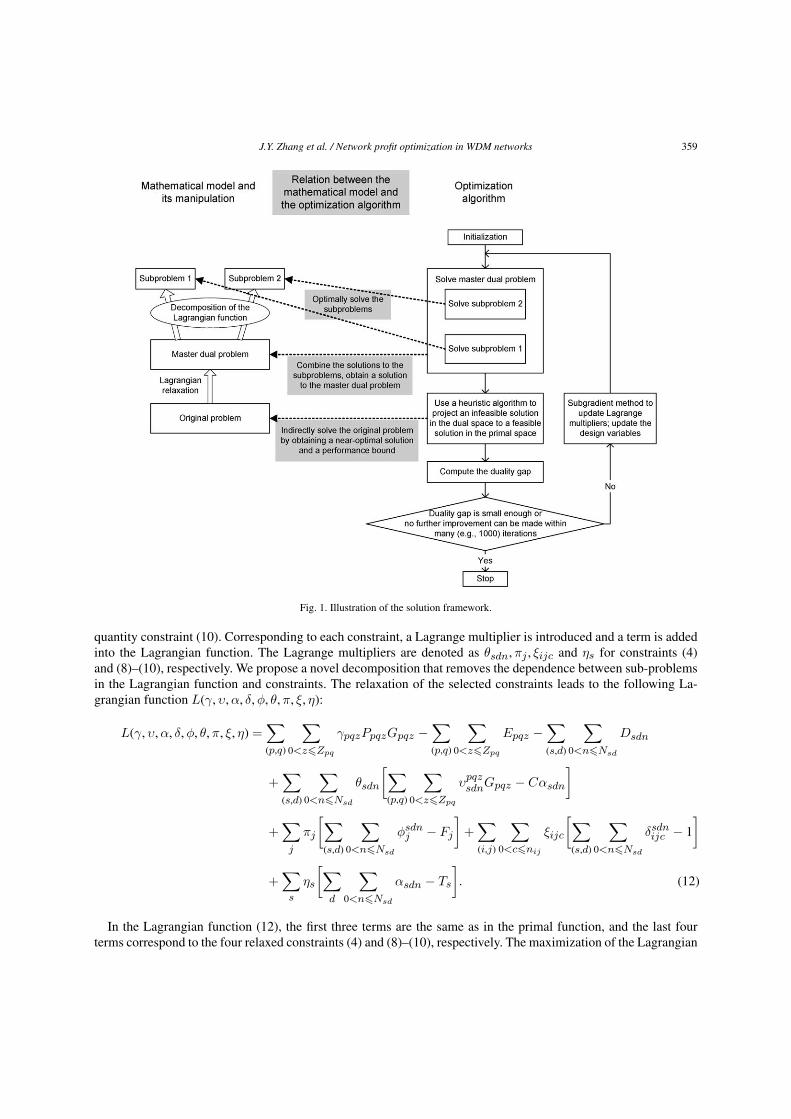
3.1. Overview of the solution framework

Our optimization method relies on the theoretical groundwork in Section 3.2 for the decomposition into lesscomplex sub-problems. By relaxing selected constraints, and transforming the relaxed constraints into soft “price”terms, we derive a Lagrangian function [20], in which Lagrange multipliers (soft “prices”) are used to reflect therelaxed hard constraints. We define a dual function as the supremum of the Lagrangian function. A dual problemis created as minimizing the dual function. During the subgradient-based iterations of solving a dual problem,the optimization process is gradually guided to respect the relaxed constraints. Such iterations have been provedto converge to the optimum (see Section 6.3.1 of [21]). The overall algorithm is an optimization procedure. Theheuristic algorithm in the optimization framework serves only as a projection from the dual space (consisting ofthe variables for the dual problem, i.e., the Lagrangian multipliers) to the primal space (consisting of the designvariables for the profit optimization problem). Strictly obeying the relaxed constraints is guaranteed in the projec-tion of an infeasible solution to a feasible solution by a heuristic algorithm. The solution framework is illustratedin Fig. 1.

Our method can solve the optimization problem for practical scale networks. CPLEX is able to obtain the optimalsolution of this problem for very small networks, but cannot solve this problem for practical networks. Existingheuristic algorithms cannot obtain a quantitative performance bound. Thus, the performance of heuristics is neverchecked for any practical network. Our method obtains a performance bound for the profit optimization problemfor practical scale networks. We prove that the minimal dual value is an upper bound for the primal function.

There is a duality gap between the minimal dual value (i.e., value for the dual function) and the maximal pri-mal value (i.e., value for the primal function). The maximal primal value represents the best achievable profit. Itcorresponds to a feasible provisioning scheme. The duality gap indicates the optimality of the solutions. A goodnear-optimal solution leads to a small duality gap.

3.2. Decomposition of the profit optimization problem

We relax selected constraints to derive a Lagrangian function, and decompose the profit optimization probleminto sub-problems. The constraints that we choose to relax are the lightpath bandwidth constraint (4), the wave-length converter quantity constraint (8), the wavelength channel exclusive usage constraint (9), and the transmitter

J.Y. Zhang et al. / Network profit optimization in WDM networks 359

Fig. 1. Illustration of the solution framework.

quantity constraint (10). Corresponding to each constraint, a Lagrange multiplier is introduced and a term is addedinto the Lagrangian function. The Lagrange multipliers are denoted as θsdn, πj , ξijc and ηs for constraints (4)and (8)–(10), respectively. We propose a novel decomposition that removes the dependence between sub-problemsin the Lagrangian function and constraints. The relaxation of the selected constraints leads to the following La-grangian function L(γ, υ, α, δ, φ, θ, π, ξ, η):

L(γ, υ, α, δ, φ, θ, π, ξ, η) =∑(p,q)

∑0<z�Zpq

γpqzPpqzGpqz −∑(p,q)

∑0<z�Zpq

Epqz −∑(s,d)

∑0<n�Nsd

Dsdn

+∑(s,d)

∑0<n�Nsd

θsdn

[∑(p,q)

∑0<z�Zpq

υpqzsdnGpqz − Cαsdn

]

+∑j

πj

[∑(s,d)

∑0<n�Nsd

φsdnj − Fj

]+

∑(i,j)

∑0<c�nij

ξijc

[∑(s,d)

∑0<n�Nsd

δsdnijc − 1

]

+∑s

ηs

[∑d

∑0<n�Nsd

αsdn − Ts

]. (12)

In the Lagrangian function (12), the first three terms are the same as in the primal function, and the last fourterms correspond to the four relaxed constraints (4) and (8)–(10), respectively. The maximization of the Lagrangian

360 J.Y. Zhang et al. / Network profit optimization in WDM networks

function is subject to the remaining constraints that are not relaxed, i.e., constraints (5)–(7) and (11).We define the dual function q(θ, π, ξ, η) as the supremum of the Lagrangian function (12). The design variables

of the dual problem are the Lagrange multipliers θ, π, ξ and η. In Appendix A, we prove the following inequality(13), and also prove that the minimum of the dual function is an upper bound of the primal function.

minθ,π,ξ,η�0

q(θ, π, ξ, η) � maxγ,υ,α,δ,φ

L(γ, υ, α, δ, φ, θ, π, ξ, η). (13)

After manipulation and re-grouping of the Lagrangian function, we create solvable and separable sub-problems.The details of the manipulation and re-grouping are given in Appendix B. The maximization of the Lagrangianfunction is transformed to:

∑(s,d)

∑0<n�Nsd

maxαsdn

{αsdn

[Hsdn − min

δ,φ(Qsdn)

]}

+∑(p,q)

∑0<z�Zpq

maxγpqz

{γpqz

[PpqzGpqz − min

υ(Rpqz)

]}− U , (14)

where

Hsdn = −Cθsdn + ηs − ts − rd, (15)

Qsdn =∑(i,j)

∑0<c�W

δsdnijc (dijc − ξijc) +

∑j

φsdnj (cj − πj), (16)

Rpqz =∑(s,d)

∑0<n�Nsd

υpqzsdn(Vpqz − θsdnGpqz), (17)

U =∑(i,j)

∑0<c�W

ξijc +∑s

ηsTs. (18)

Since the re-grouped Lagrangian function is decomposable, the maximization of the Lagrangian function can bedecomposed into sub-problems. There are three groups in (14):

• The first group of (14) represents the design of the lightpath setup status α, the lightpath routing and wave-length assignment scheme δ, and the assignment scheme of wavelength converters to lightpaths δ. We call itthe RWA sub-problem;

• The second group of (14) represents the design of the traffic flow admission status γ, and the traffic flowrouting scheme υ. We call it the traffic flow routing sub-problem;

• The last group of (14) is independent of any design variables.

3.3. Solving the sub-problems

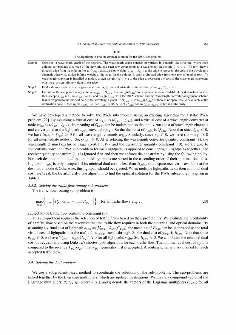
3.3.1. Solving the RWA sub-problemThe RWA sub-problem is described as:

maxαsdn

{αsdn

[Hsdn − min

δ,φ(Qsdn)

]}for all lightpaths ssdn, (19)

subject to the lightpath flow continuity constraints (6), the wavelength conversion constraint (7) and the receiverquantity constraint (11).

J.Y. Zhang et al. / Network profit optimization in WDM networks 361

Table 1

The algorithm to find the optimal solution for the RWA sub-problem

Step 1: Construct a wavelength graph of the network. The wavelength graph consists of vertices in a matrix-like structure, where eachcolumn corresponds to a node of the network, and each row corresponds to a wavelength. In the cth (0 < c � W ) row, draw adirected edge from the column i to j, if wijc exists, assign weight (dijc − ξijc) to the edge to represent the cost of the wavelengthchannel; otherwise, assign infinite weight to the edge. In the column i, draw a directed edge from one row to another row, if awavelength converter is installed at node i, assign weight (ci − πi) to the edge to represent the cost of the wavelength converter;otherwise, assign infinite weight to the edge

Step 2: Find a shortest path between a given node pair (s, d), and calculate the optimal value of minδ,φ(Qsdn)

Step 3: Determine the acceptance or rejection of ssdn. If Hsdn > minδ,φ(Qsdn) and a spare receiver is available at the destination node d,then accept ssdn (i.e., set αsdn = 1), and assign ssdn with the RWA scheme and the wavelength converter assignment schemethat correspond to the shortest path in the wavelength graph. If Hsdn < minδ,φ(Qsdn) or there is no spare receiver available at thedestination node d, then reject ssdn (i.e., set αsdn = 0). A tie of Hsdn and minδ,φ(Qsdn) is broken arbitrarily

We have developed a method to solve the RWA sub-problem using an existing algorithm for a static RWAproblem [22]. By assuming a virtual cost of wijc as (dijc − ξijc), and a virtual cost of a wavelength converter atnode wijc as (dijc − ξijc), the meaning of Qsdn can be understood as the total virtual cost of wavelength channelsand converters that the lightpath ssdn travels through. So the dual cost of ssdn is Qsdn. Note that since ξijc � 0,we have (dijc − ξijc) � 0 for all wavelength channels wijc. Similarly, since πj � 0, we have (cj − πj) � 0for all intermediate nodes j. So, Qsdn � 0. After relaxing the wavelength converter quantity constraint (8), thewavelength channel exclusive usage constraint (9), and the transmitter quantity constraint (10), we are able tosequentially solve the RWA sub-problem for each lightpath, as opposed to considering all lightpaths together. Thereceiver quantity constraint (11) is ignored first and then we enforce the constraint by using the following policy.For each destination node d, the obtained lightpaths are sorted in the ascending order of their minimal dual cost.Lightpath ssdn is only accepted, if its minimal dual cost is less than Hsdn, and a spare receiver is available at thedestination node d. Otherwise, this lightpath should be rejected. When multiple lightpaths tie on their minimal dualcost, we break the tie arbitrarily. The algorithm to find the optimal solution for the RWA sub-problem is given inTable 1.

3.3.2. Solving the traffic flow routing sub-problemThe traffic flow routing sub-problem is:

maxγpqz

{γpqz

[PpqzGpqz − min

υ(Rpqz)

]}for all traffic flows χpqz , (20)

subject to the traffic flow continuity constraint (5).This sub-problem requires the selection of traffic flows based on their profitability. We evaluate the profitability

of a traffic flow based on the resources that the traffic flow requires in both the electrical and optical domains. Byassuming a virtual cost of lightpath ssdn as (Vpqz −θsdnGpqz), the meaning of Rpqz can be understood as the totalvirtual cost of lightpaths that the traffic flow χpqz travels through. So the dual cost of χpqz is Rpqz . Note that sinceθsdn � 0, we have (Vpqz − θsdnGpqz) � 0 for all lightpaths ssdn. So, Rpqz � 0. We can obtain the minimal dualcost by sequentially using Dijkstra’s shortest path algorithm for each traffic flow. The minimal dual cost of χpqz iscompared to the revenue PpqzGpqz that χpqz generates if it is accepted. A routing scheme υ is obtained for eachaccepted traffic flow.

3.4. Solving the dual problem

We use a subgradient-based method to coordinate the solutions of the sub-problems. The sub-problems arelinked together by the Lagrange multipliers, which are updated in iterations. We create a compound vector of theLagrange multipliers (θ, π, ξ, η), where θ, π, ξ and η denote the vectors of the Lagrange multipliers (θsdn) for all

362 J.Y. Zhang et al. / Network profit optimization in WDM networks

lightpaths ssdn, (πj) for all intermediate nodes j, (ξijc) for all wavelength channels wijcand (ηs) for all sourcenodes s. We update (θ, π, ξ, η) in iterations towards the direction of its subgradient.

(θ, π, ξ, η)(h+1) = (θ, π, ξ, η)(h) + β(h)g((θ, π, ξ, η)(h)), (21)

where (θ, π, ξ, η)(h) denotes the value of vectors (θ, π, ξ, η) obtained in the hth iteration, and β(h) denotes the stepsize for the (h + 1)th iteration.

The subgradient of q in Eq. (13) is denoted as (g(θ), g(π), g(ξ), g(η)). The vectors g(θ), g(π), g(ξ) and g(η)comprise (g(θsdn)) for all lightpaths ssdn, (g(πj)) for all intermediate nodes j, (g(ξijc)) for all wavelength channelswijc and (g(ηs)) for all source nodes s, respectively. We have the subgradient components:

g(θsdn) =∑(p,q)

∑0<z�Zpq

υpqzsdnGpqz − Cαsdn for all lightpaths ssdn, (22)

g(πj) =∑(s,d)

∑0<n�Nsd

φsdnj − Fj for all intermediate nodes j, (23)

g(ξijc) =∑(s,d)

∑0<n�Nsd

δsdnijc − 1 for all wavelength channels wijc, (24)

g(ηs) =∑d

∑0<n�Nsd

αsdn − Ts for all source nodes s. (25)

The subgradient terms in Eqs (22)–(25) correspond to the relaxed constraints (4) and (8)–(10).The step size for the iterative updates is computed as

β(h) = μ × qU − q(h)

gT ((θ, π, ξ, η)(h))g((θ, π, ξ, η)(h)), (26)

where qU is an approximation to the optimal dual value. We set an initial estimation of qU to the value of theobjective function f for a feasible solution. q(h) is the value of the dual function q at the hth iteration. The rangeof the parameter μ is 0 < μ < 2, which is adjusted adaptively as the algorithm converges. Specifically, if thevalue of q(h) remains unchanged in 3 consecutive iterations, the value of μ is decreased by a factor p < 1, andif the value of q(h) increases in 5 consecutive iterations, the value of μ is increased by a factor 1/p. From oursimulation, fast convergence is achieved when p = 0.95. The vector gT((θ, π, ξ, η)(h)) is the transpose of the vectorg((θ, π, ξ, η)(h)). The value qU is also updated when a lower f value is obtained.

3.5. Constructing a feasible solution

A heuristic algorithm is developed to construct a feasible solution for the primal problem. Because some con-straints for the primal problem are relaxed and transformed into the price terms in the dual problem, the solutionto the dual problem is generally infeasible, i.e., some constraints are violated. Our heuristic algorithm repeatedlydiverts the least profitable traffic flows and the traffic flows along the least profitable lightpaths onto other existinglightpaths, until all conflicts are resolved. The description of the heuristic algorithm is given in Table 2.

3.6. Computational complexity analysis

The computational complexities to solve the traffic flow routing and RWA sub-problems are O(A(N+W )N2W )and O(ZA2N2), respectively, where A is the total number of potential lightpaths to be set up; N is the number

J.Y. Zhang et al. / Network profit optimization in WDM networks 363

Table 2

A heuristic algorithm to construct a feasible solution for the primal problem

1.0 (Rough searching stage. Transform an infeasible RWA scheme obtained in the dual solution to a feasible but not very optimized RWAscheme. At the same time, obtain a rough traffic routing scheme, which is feasible but far from being optimized.)

1.1 (Initial RWA. Deploy lightpaths one-by-one.)

1.1.1 (Choose the top priority lightpath from the lightpaths that have not been deployed or rejected. If two lightpaths tie on the firstpriority, use the second priority and then the third priority to break the tie; if still tie, break the tie randomly.)

Priority 1: Descending order of the profit of a lightpath in the dual problem, which is calculated by subtracting the dual costQsdn of the lightpath ssdn from the total revenue of the unsatisfied traffic flows between (s, d). The total revenue ofthe unsatisfied traffic flows between (s, d) is estimated as the total revenue of the traffic flows between (s, d) minusm × 0.8 × C, where m is the number of existing lightpaths between (s, d), and C is the capacity of a lightpath.Here, we assume existing lightpaths use 80% capacity to carry traffic flows;

Priority 2: Ascending order of the number of the constraints that are violated by a lightpath;Priority 3: If a lightpath is set up in the dual solution, then it has higher priority than the lightpath that is not set up in the dual

solution.

1.1.2 (Deploy the top priority lightpath. Use the first policy to deploy the lightpath, if the required resources are available so far. Iffailed, use the second policy and then the third policy. If still failed, reject the lightpath.)

Policy 1: Deploy the lightpath based on its RWA scheme obtained in the dual solution;Policy 2: Deploy the lightpath based on its routing scheme obtained in the dual solution, but choose a different wavelength

assignment scheme;Policy 3: Compute a new relatively low cost RWA scheme for the lightpath.

1.1.3 If there are lightpaths that have not been deployed or rejected, then repeat from Step 1.1.1.

1.2 (Traffic routing.)

1.2.1 (Sort traffic flows. If two traffic flows tie on the first priority, use the second priority and then the third priority to break the tie;if still tie, break the tie arbitrarily.)

Priority 1: Descending order of the profit of a traffic flow per bandwidth unit, which is calculated by subtracting the dual costRpqz of χpqz from its revenue PpqzGpqz , then dividing by its bandwidth requirement Gpqz ;

Priority 2: Ascending order of the number of the constraints that are violated by a traffic flow;Priority 3: Descending order of the bandwidth requirement Gpqz of χpqz .

1.2.2 (Deploy traffic flows one-by-one based on the sorted order. Use the first policy to deploy a traffic flow, if the required resourcesare available so far. If failed, use the second policy. If still failed, then reject the traffic flow.)

Policy 1: Deploy a traffic flow based on its traffic routing scheme obtained in the dual solution.Policy 2: Compute a new relatively low cost traffic routing scheme for traffic flow.

1.3 (RWA adjustment.)

1.3.1 Remove non-profitable lightpaths.1.3.2 Re-route the traffic flows that use the disconnected lightpaths. If not re-routed, then reject the traffic flows.

2.0 (Extensive searching stage. Optimize the traffic routing scheme based on the virtual topology obtained in the previous rough searchingstage.)

Use the Lagrangian relaxation and subgradient methods to solve the optimization problem:

maxγ,υ

(f ), where f =∑(p,q)

∑0<z�Zpq

γpqzPpqzGpqz −∑(p,q)

∑0<z�Zpq

Epqz . (27)

Subject to the lightpath capacity constraint (4), and the traffic flow continuity constraint (5). The solution method of this optimizationproblem is available in [23].

364 J.Y. Zhang et al. / Network profit optimization in WDM networks

of nodes; and Z is the number of traffic flows. Thus the computation complexity to solve the dual problem isO(A(N + W )N2W ) + O(ZA2N2). The dual problem needs to be solved for many iterations in the overall frame-work. The good convergence of the subgradient-based iterations keeps the computational complexity of the overalloptimization approach at an acceptable level. Our simulation on practical scale networks demonstrates the effi-ciency of the approach.

4. Numeric results

4.1. Verification of the proposed solution method

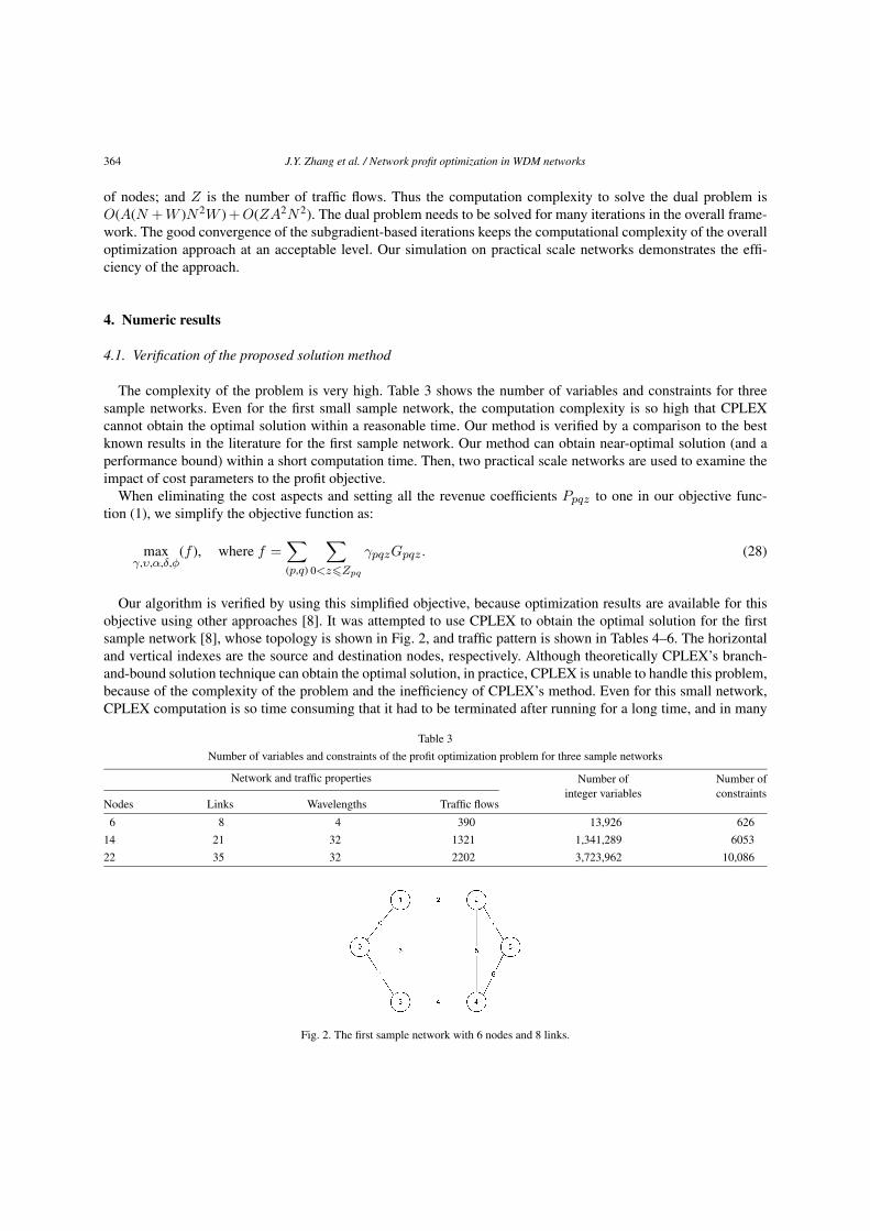
The complexity of the problem is very high. Table 3 shows the number of variables and constraints for threesample networks. Even for the first small sample network, the computation complexity is so high that CPLEXcannot obtain the optimal solution within a reasonable time. Our method is verified by a comparison to the bestknown results in the literature for the first sample network. Our method can obtain near-optimal solution (and aperformance bound) within a short computation time. Then, two practical scale networks are used to examine theimpact of cost parameters to the profit objective.

When eliminating the cost aspects and setting all the revenue coefficients Ppqz to one in our objective func-tion (1), we simplify the objective function as:

maxγ,υ,α,δ,φ

(f ), where f =∑(p,q)

∑0<z�Zpq

γpqzGpqz . (28)

Our algorithm is verified by using this simplified objective, because optimization results are available for thisobjective using other approaches [8]. It was attempted to use CPLEX to obtain the optimal solution for the firstsample network [8], whose topology is shown in Fig. 2, and traffic pattern is shown in Tables 4–6. The horizontaland vertical indexes are the source and destination nodes, respectively. Although theoretically CPLEX’s branch-and-bound solution technique can obtain the optimal solution, in practice, CPLEX is unable to handle this problem,because of the complexity of the problem and the inefficiency of CPLEX’s method. Even for this small network,CPLEX computation is so time consuming that it had to be terminated after running for a long time, and in many

Table 3

Number of variables and constraints of the profit optimization problem for three sample networks

Network and traffic properties Number ofinteger variables

Number ofconstraints

Nodes Links Wavelengths Traffic flows

6 8 4 390 13,926 626

14 21 32 1321 1,341,289 6053

22 35 32 2202 3,723,962 10,086

Fig. 2. The first sample network with 6 nodes and 8 links.

J.Y. Zhang et al. / Network profit optimization in WDM networks 365

Table 4

Traffic flows of 1 bandwidth unit for the first sample network

0 5 4 11 12 9

0 0 8 5 16 6

14 12 0 9 6 16

4 11 15 0 1 5

10 2 3 3 0 9

2 1 8 15 13 0

Table 5

Traffic flows of 3 bandwidth units for the first sample network

0 6 2 1 5 4

8 0 8 6 7 8

1 3 0 0 2 7

5 7 3 0 2 6

6 4 5 0 0 2

5 4 4 2 0 0

Table 6

Traffic flows of 12 bandwidth units for the first sample network

0 1 1 1 0 0

1 0 1 1 0 2

0 1 0 2 1 0

2 0 2 0 2 0

1 2 0 2 0 1

1 1 2 2 2 0

Table 7

A comparison between our results and the published results

Near-optimal results by Maximizing Maximizing The results The upper

terminating CPLEX single-hop resource obtained by our bound

computations after a long traffic heuristics utilization proposed obtained by

running time results heuristics results method our method

T = 2, W = 3 – – – 516 576

T = 3, W = 3 738 701 666 751 851

T = 4, W = 4 927 883 925 930 976

T = 5, W = 3 967 933 933 969 987

T = 7, W = 3 967 933 933 969 987

T = 3, W = 4 738 701 666 751 851

T = 4, W = 4 933 920 925 930 976

T = 5, W = 4 988 988 988 988 988

Note: Larger optimization results mean better throughput. The first three columns are the best known results in the literature.

cases no optimal solution was obtained in [8]. Our method uses a reasonable computational time (about 10 minutesfor this sample network) to obtain comparable results (shown in Table 7). It is assumed that all nodes have the samenumber of transmitters and receivers, i.e., Ti = Ri = T for all node i. In addition, we obtain an upper bound ofthe objective function at the same time.

366 J.Y. Zhang et al. / Network profit optimization in WDM networks

4.2. Optimization results for practical scale networks

We study the impact of cost parameters to the profit for NSFNET, whose topology is shown in Fig. 3. Therandomly generated traffic pattern is shown in Tables 8–10. We found that the uniformly distributed traffic patternis more challenging than other special patterns. Therefore, we evaluate our algorithm for the uniform traffic pattern.We fix other cost parameters and investigate the impact of a single cost parameter. Between each node pair, thereare traffic flows with three different bandwidths. Our algorithm accepts or rejects traffic flows between the samenode pair independently based on the profit objective. The accepted traffic flows are allowed to use different trafficrouting schemes.

We study the impact of the number of transmitters and receivers on the profit. It is assumed that all nodeshave the same number of transmitters and receivers, i.e., Ti = Ri = T for all node i. For now, we do notconsider the traffic grooming cost V . All revenue coefficients Ppqz are set to one, which means the revenue isproportional to the bandwidth requirement. Since the total traffic volume counts to 6148 bandwidth units, themaximal revenue is 6148, if all the traffic flows are accepted. Figure 4 illustrates the achieved profit and its upperbound with respect to the number of transmitters at a node. We can see that as the number of transmitters increases,the profit increases. The increasing rate of profit is approximately linear to the number of transmitters before thetransmitters become abundant. After that, adding more transmitters increases the cost but contributes no additionalrevenue. The profit decreases at a rate approximately linear to the transmitter cost. In this way, the optimal numberof transmitters at a node is obtained for a given traffic pattern. Figure 5 shows the percentage of the rejectedtraffic flows as the transmitter cost increases. The number of transmitters and receivers at a node is set to the

Fig. 3. 14-node NSFNET topology.

Table 8

Traffic flows of 1 bandwidth unit for NSFNET (total 541 flows)

0 6 3 12 5 1 6 0 2 0 4 2 0 3

0 0 2 2 2 11 1 1 1 2 3 0 1 3

3 2 0 3 0 1 2 3 11 3 1 2 2 0

3 1 4 0 11 1 2 3 2 2 1 2 1 3

1 3 0 2 0 4 0 2 0 3 0 1 1 3

1 2 1 3 2 0 1 3 3 11 0 6 10 9

2 2 3 1 10 3 0 0 3 1 2 0 3 7

3 10 2 3 5 4 1 0 0 3 2 0 3 0

3 0 12 3 3 3 1 0 0 2 1 7 9 0

0 0 0 1 2 0 2 0 1 0 1 0 0 4

4 0 0 10 0 3 0 6 0 3 0 3 5 3

2 3 1 1 3 2 13 2 10 2 2 0 1 3

13 0 11 2 0 1 2 0 9 0 2 1 0 3

10 14 0 15 9 3 1 3 0 12 2 1 3 0

J.Y. Zhang et al. / Network profit optimization in WDM networks 367

Table 9

Traffic flows of 3 bandwidth units for NSFNET (total 417 flows)

0 1 2 1 3 1 0 2 2 0 3 2 0 4

3 0 0 2 2 2 1 1 1 2 3 0 1 6

1 2 0 1 0 2 2 3 1 2 3 8 6 7

6 1 0 0 1 3 2 1 2 2 1 2 1 8

1 2 7 2 0 1 0 2 0 6 0 8 2 5

5 4 1 1 2 0 1 1 3 4 0 1 1 2

2 5 7 8 1 2 0 0 3 1 2 0 0 5

2 3 2 1 3 4 5 0 0 1 2 0 7 6

1 0 5 5 2 1 2 0 0 2 1 3 1 2

0 0 6 1 2 0 2 0 3 0 2 0 0 1

1 4 7 3 0 0 3 3 0 1 0 1 1 2

2 3 2 5 6 7 8 2 2 2 2 0 1 1

0 0 1 2 2 3 4 0 1 0 3 5 0 7

4 3 0 2 3 3 3 1 0 4 7 1 0 0

Table 10

Traffic flows of 12 bandwidth units for NSFNET (total 363 flows)

0 2 5 3 5 4 2 1 2 5 2 1 5 0

4 0 4 1 4 3 2 5 3 4 3 3 1 3

0 1 0 0 0 2 3 0 5 3 2 1 0 2

1 1 0 0 3 1 1 0 2 4 4 3 1 4

3 0 0 2 0 3 5 2 4 2 5 4 0 3

1 3 2 0 1 0 2 0 0 1 0 1 5 2

1 4 0 4 0 0 0 0 4 3 1 2 2 1

0 3 1 0 5 0 4 0 0 0 3 0 4 0

0 4 1 2 3 5 1 4 0 2 1 5 4 0

5 1 0 1 1 4 0 0 1 0 1 0 0 1

1 3 3 0 4 3 1 2 0 0 0 0 1 3

1 0 2 2 5 1 0 3 3 3 2 0 3 5

0 5 2 3 4 1 2 0 2 1 1 1 0 3

5 2 5 5 1 0 2 0 1 4 0 1 0 0

optimal value 9 that is obtained in Fig. 4. It is assumed that the transmitter cost and the receiver cost are thesame.

We next study the impact of the wavelength channel cost. With an increase of the wavelength channel cost, thetotal number of the established lightpaths decreases (shown in Fig. 6). When the wavelength channel cost increasesfrom 0 to 9, the total number of established lightpaths decreases by (119−88)/119 = 26%. The reason is that morelightpaths become non-profitable as the wavelength channel cost increases. The remaining profitable traffic flowstend to be packed into a smaller number of lightpaths. An increase of the wavelength channel cost dramaticallyreduces the lightpaths that use multiple fibre hops. In Fig. 7, we show that the percentage of 3-fibre hop lightpathsis reduced from 45 to 23%, as the wavelength channel cost increases from 0 to 9. This is because more lightpaths ofsingle fibre hop are established when the wavelength channel cost is high. The proportion of single-hop lightpathsincreases from 18 to 41%, as the wavelength channel cost increases from 0 to 9.

We study the impact of the traffic grooming cost. The optical layer cost is fixed. The traffic grooming costis modelled by the coefficient Vpqz . We set Vpqz to a fraction of the bandwidth requirement Gpqz of χpqz . Ta-ble 11 shows the number of the accepted traffic flows with different bandwidths. When the traffic grooming

368 J.Y. Zhang et al. / Network profit optimization in WDM networks

Fig. 4. Profit and an upper bound w.r.t. the number of transmitters at a node.

Fig. 5. Percentage of the rejected traffic flows w.r.t. the transmitter cost.

cost Vpqz increases from 0 to 0.6Gpqz , the traffic flows with different bandwidths exhibit dramatically differ-ent behaviours: (1) for large bandwidth (i.e., OC-12) traffic flows, the number of traffic flows using multiple hoplightpath decreases significantly, by (29 − 7)/29 = 76%; the number of traffic flows using single hop light-path slightly decreases, by (261 − 250)/261 = 4%. It is more efficient to carry them by single hop lightpaths;(2) for medium bandwidth (i.e., OC-3) traffic flows, the number of traffic flows using multiple hop lightpathsdecreases by (81 − 59)/81 = 27%; the number of traffic flows using single hop lightpath increases slightly, by(274 − 246)/246 = 11%. More lightpaths should be set up so that more such traffic flows can be carried oversingle hop lightpaths. However, the revenue generated by such traffic flows remains at the same level; (3) for smallbandwidth (i.e., OC-1) traffic flows, the number of traffic flows using multiple hop lightpaths increases signifi-cantly, by (139 − 45)/45 = 209%; the number of traffic flows using single hop lightpaths approximately remainsthe same. More such traffic flows are accepted by using multiple hop lightpaths (particularly two hop lightpaths).

J.Y. Zhang et al. / Network profit optimization in WDM networks 369

Fig. 6. Number of the established lightpaths of different fibre hops w.r.t. the wavelength channel cost.

Fig. 7. Percentage of single-hop and multiple-hop lightpaths in all established lightpaths w.r.t. the wavelength channel cost.

Table 11

Total number of the accepted traffic flows of different bandwidth

Traffic flow bandwidth Lightpath hop Vpqz = 0 Vpqz = 0.6 × Gpqz

OC-12 (Total 363 traffic flows) 1 261 250

2 29 7

3 0 0

4 0 0

OC-3 (Total 417 traffic flows) 1 246 274

2 81 59

3 3 1

4 0 0

OC-1 (Total 541 traffic flows) 1 350 352

2 45 139

3 9 9

4 1 0

370 J.Y. Zhang et al. / Network profit optimization in WDM networks

Fig. 8. Average lightpath hops of OC-3 traffic flows w.r.t. their traffic grooming cost.

The reason is that such traffic flows use the segregated bandwidth that cannot be used by medium and large band-width traffic flows. Since we assume that the traffic grooming cost is proportional to the bandwidth requirement,the traffic grooming cost for small bandwidth traffic flows is not a major cost compared to other costs such as theoptical layer cost.

We study the ratio of optical pass-through traffic at a node with respect to the traffic grooming cost. We fixthe traffic grooming cost Vpqz for OC-1 and OC-12 traffic flows to 0.1 and 1.2, respectively, and vary Vpqz forOC-3 traffic flows. We observe that as Vpqz increases, the average number of lightpath hops of OC-3 traffic flowsdecreases (shown in Fig. 8). When Vpqz reaches 1.5, all OC-3 traffic flows are carried over single hop lightpaths.The reason is that the revenue of an OC-3 traffic flow is 3 when Ppqz = 1. When Vpqz reaches 1.5, the trafficflows cannot afford to take two lightpath hops anymore. Since the vast majority of OC-3 traffic flows are carriedby single hop or two-hop lightpaths as shown in Table 11, we have the rough relation of the average lightpath hopnumber and the percentage of optical pass-through traffic flows:

Average lightpath hop number of a traffic flow

= 1 + (Optical passthrough traffic flows at a node)%. (29)

The results in Fig. 8 indicate that about 15–20% OC-3 traffic flows optically pass through intermediate nodes,when the Vpqz is below 1.5. The remaining 80–85% OC-3 traffic flows exit from add-drop ports of an opticalswitch. They either reach their final destination, or are re-groomed with other traffic flows and re-enter the opticaldomain again.

Our results show that when wavelength converters are used, their contribution to the profit objective is negligible.In Table 12, the influence of the number of wavelength converters at a node on the profit objective is shown.Compared to the counter cases of no wavelength converters, the profit improvement is marginal.

For most cases in the second sample network, our method can compute results within 2 hours on a PC configuredwith a 1.4 GHz Intel® CPU, 512 MB RAM and the Windows XP® operating system.

We study the network profit optimization problem for the third sample network. This network has 22 nodes,35 links and 32 wavelengths on each link. The topology is shown in Fig. 9. The uniform traffic patternis shown in Tables 13–15, counting to 2202 traffic flows in total. The trafficg grooming problem in WDM

J.Y. Zhang et al. / Network profit optimization in WDM networks 371

Table 12

Influence of the number of wavelength converters at a node on the profit objective

W Ti, Ri dijc ri, ti Vpqz Fi ci f

OC-1 OC-3 OC-12

32 9 0 7 0 0 0 0 0 1402

32 9 0 7 0 0 0 1 0.01 1413

32 9 0.2 7 0 0 0 0 0 1386

32 9 0.2 7 0 0 0 1 0.01 1388

32 9 3 7 0 0 0 0 0 690

32 9 3 7 0 0 0 1 0.01 699

32 9 3 7 0.1 0.3 1.2 0 0 127

32 9 3 7 0.1 0.3 1.2 1 0.01 127

Fig. 9. The third sample network with 22 nodes and 35 links.

networks has never been studied for such large networks before, because the limitation of the existing op-timization algorithm. Our method can compute a feasible solution and a performance bound within 5–6hours. In Fig. 10, we show that the network profit decreases as the cost of a transmitter and receiver in-creases.

5. Conclusions

In this study of static traffic grooming in WDM networks, we have modeled the profit as the surplus of therevenue generated by the accepted traffic flows over resource costs. With a profit optimization objective that incor-porates both cost minimization and throughput maximization objectives, we can identify profitable traffic flows,and provide optimized provisioning schemes for the accepted traffic flows. Using the LR and subgradient meth-ods, we can solve the optimization problem for fairly large networks. Our approach can obtain an upper boundto evaluate the optimality of the feasible solution. A comparison between our results and the published resultsdemonstrates the effectiveness of our approach. In studying a practical-size network, we have observed differentbehaviours and contributions to the profit objective by different bandwidth traffic flows, and when the relative costof electrical and optical layers changes. In addition, our study has shown that the use of wavelength converters haslittle contribution to the profit objective for static traffic patterns.

372 J.Y. Zhang et al. / Network profit optimization in WDM networks

Table 13

Traffic flows of 1 bandwidth unit for the third sample network

0 6 3 12 5 1 6 0 2 0 4 2 0 3 6 0 2 0 4 2 0 3

0 0 2 2 2 11 1 1 1 2 3 0 1 3 3 0 2 0 4 0 2 6

3 2 0 3 0 1 2 3 11 3 1 2 2 0 1 3 0 2 0 4 0 2

3 1 4 0 11 1 2 3 2 2 1 2 1 3 3 1 10 3 0 0 3 1

1 3 0 2 0 4 0 2 0 3 0 1 1 3 0 9 3 1 3 0 12 7

1 2 1 3 2 0 1 3 3 11 0 6 10 9 3 1 4 0 11 1 2 3

2 2 3 1 10 3 0 0 3 1 2 0 3 7 2 3 5 4 1 0 0 4

3 10 2 3 5 4 1 0 0 3 2 0 3 0 3 1 1 3 2 0 2 10

3 0 12 3 3 3 1 0 0 2 1 7 9 0 11 2 0 1 2 0 9 0

0 0 0 1 2 0 2 0 1 0 1 0 0 4 6 0 3 0 3 5 3 0

4 0 0 10 0 3 0 6 0 3 0 3 5 3 0 2 2 2 11 1 1 1

2 3 1 1 3 2 0 2 10 2 2 0 1 3 2 1 2 1 3 3 1 0

0 0 11 2 0 1 2 0 9 0 2 1 0 3 2 2 1 2 1 3 3 1

10 0 0 0 9 3 1 3 0 12 2 1 3 0 3 2 0 2 10 2 2 2

3 11 0 6 10 9 3 1 4 0 1 0 0 2 0 7 9 0 11 2 1 0

2 0 2 0 1 0 1 0 0 4 6 0 3 0 3 0 1 0 1 0 0 1

0 1 2 3 11 3 1 2 2 0 1 3 0 2 0 4 0 2 11 1 1 2

3 2 0 3 0 1 2 3 11 3 1 2 0 1 3 3 0 0 0 6 0 3

0 2 0 3 0 1 1 0 11 1 2 3 2 2 11 3 0 2 0 4 0 8

8 0 2 10 2 2 1 4 0 1 0 0 2 0 11 0 6 10 9 0 1 0

0 0 3 2 0 3 0 3 1 0 2 0 1 0 1 0 0 2 0 1 0 2

3 1 2 2 0 1 3 0 12 3 3 3 1 0 0 2 10 9 3 1 4 0

Table 14

Traffic flows of 3 bandwidth units for the third sample network

0 1 2 1 3 1 0 2 2 0 3 2 0 4 0 2 0 0 0 0 2 0

3 0 0 2 2 2 1 1 1 2 3 0 1 0 3 0 0 2 2 2 1 3

1 2 0 1 0 2 2 3 1 2 3 0 0 0 1 0 0 1 3 2 1 2

0 1 0 0 1 3 2 1 2 2 1 2 1 0 0 0 0 1 2 0 0 3

1 2 0 2 0 1 0 2 0 0 0 0 2 0 0 0 0 2 1 2 0 0

0 4 1 1 2 0 1 1 3 4 0 1 1 2 1 2 2 3 4 0 1 0

2 0 0 0 1 2 0 0 3 1 2 0 0 0 0 2 1 2 0 0 2 4

2 3 2 1 3 4 0 0 0 1 2 0 0 0 0 0 1 2 0 2 1 2

1 0 0 0 2 1 2 0 0 2 1 3 1 2 3 2 0 0 0 0 2 2

0 0 0 1 2 0 2 0 3 0 2 0 0 1 2 2 1 1 1 2 3 3

1 4 0 3 0 0 3 3 0 1 0 1 1 2 3 2 0 4 0 2 0 0

2 3 2 0 0 0 0 2 2 2 2 0 1 1 0 1 0 2 2 3 1 2

0 0 1 2 2 3 4 0 1 0 3 0 0 0 2 0 1 0 2 0 0 0

4 3 0 2 3 3 3 1 0 4 0 1 0 0 0 1 2 0 0 3 1 2

2 3 2 1 3 4 0 0 0 1 2 2 1 2 0 0 0 0 2 0 0 0

3 4 0 0 0 1 2 0 0 2 0 1 1 3 4 0 1 1 2 1 2 1

0 0 1 2 0 0 0 0 0 1 2 0 2 1 4 0 0 0 1 2 0 0

1 3 2 1 2 2 1 2 1 0 0 0 2 0 2 0 1 0 2 0 0 3

0 1 1 3 4 0 1 1 2 1 2 2 0 1 1 3 4 0 0 1 2 3

2 1 2 0 0 2 1 3 1 2 3 0 1 2 0 0 0 0 0 0 1 1

2 0 0 3 1 2 0 0 0 0 2 4 0 0 0 1 2 0 0 0 0 0

2 0 0 2 1 3 1 2 3 4 0 0 0 1 2 0 3 3 0 1 0 0

J.Y. Zhang et al. / Network profit optimization in WDM networks 373

Table 15

Traffic flows of 12 bandwidth units for the third sample network

0 2 0 3 0 0 2 1 2 0 2 1 0 0 0 3 0 0 2 1 2 0

0 0 0 1 0 3 2 0 3 0 3 3 1 3 3 0 1 2 0 2 1 1

0 1 0 0 0 2 3 0 0 3 2 1 0 2 1 0 0 3 1 1 0 2

1 1 0 0 3 1 1 0 2 0 0 3 1 0 0 2 1 0 0 0 3 0

3 0 0 2 0 3 0 2 0 2 0 0 0 3 0 2 0 0 1 0 2 0

1 3 2 0 1 0 2 0 0 1 0 1 0 2 3 2 0 3 0 3 3 1

1 0 0 0 0 0 0 0 0 3 1 2 2 1 3 2 0 1 0 2 0 0

0 3 1 0 0 0 0 0 0 0 3 0 0 0 0 1 0 3 2 0 3 0

0 0 1 2 3 0 1 0 0 2 1 0 0 0 1 2 0 2 1 0 0 0

0 1 0 1 1 0 0 0 1 0 1 0 0 1 0 3 0 3 3 1 3 3

1 3 3 0 0 3 1 2 0 0 0 0 1 3 0 0 0 2 3 0 0 3

1 0 2 2 0 1 0 3 3 3 2 0 3 0 0 3 2 1 0 2 1 0

0 0 2 3 0 1 2 0 2 1 1 1 0 3 1 3 2 0 1 0 2 0

0 2 0 0 1 0 2 0 1 0 0 1 0 0 2 1 0 0 0 3 0 0

0 0 2 1 0 0 0 1 2 0 0 0 2 3 0 0 3 2 0 3 0 2

0 0 1 2 0 0 3 1 0 0 2 1 0 0 0 0 3 1 2 2 1 0

0 1 0 1 0 0 1 1 0 0 2 1 0 0 0 1 0 0 0 3 0 0

0 0 0 1 3 0 0 0 2 3 0 1 2 0 0 0 2 0 3 2 0 3

0 0 1 0 3 3 3 2 0 3 0 0 3 2 1 0 3 2 0 3 0 3

0 0 0 1 0 1 0 0 1 0 3 0 3 1 2 0 0 0 2 0 0 0

3 0 1 3 0 0 0 1 2 2 1 3 2 0 1 0 0 0 3 0 0 3

3 1 0 0 2 1 0 0 0 0 0 0 0 0 0 3 0 0 0 2 1 0

Fig. 10. Profit w.r.t. the transmitter and receiver cost for the third sample network.

Although we have provided a promising framework to solve the profit optimization problem for practical-sizenetworks, the duality gap in some cases is still large. This indicates that the feasible solution is far from theoptimal solution. Different heuristics should be investigated to reduce the duality gap. Also Our optimization isso far conducted on individual parameters, more joint optimization using multiple parameters would be desir-able.

374 J.Y. Zhang et al. / Network profit optimization in WDM networks

Appendix A. Proof of the Eq. (13)

Denote the constraints (4) and (8)–(10) as hk(γ, υ, α, δ, φ) � 0 for k = 1, 2, 3, 4, respectively.Define the Lagrangian function (12) as L(γ, υ, α, δ, φ, θ, π, ξ, η):

L(γ, υ, α, δ, φ, θ, π, ξ, η) = f (γ, υ, α, δ, φ) + θ × h1(γ, υ, α, δ, φ) + π × h2(γ, υ, α, δ, φ)

+ ξ × h3(γ, υ, α, δ, φ) + η × h4(γ, υ, α, δ, φ). (30)

Define the dual function q(θ, π, ξ, η) as the supremum of L:

q(θ, π, ξ, η) = supγ,υ,α,δ,φ

L(γ, υ, α, δ, φ, θ, π, ξ, η), θ, π, ξ, η � 0. (31)

By definition,

q(θ, π, ξ, η) � L(γ, υ, α, δ, φ, θ, π, ξ, η). (32)

When the dual function reaches its minimum and the Lagrangian function reaches it maximum, the above in-equality still holds. Thus,

minθ,π,ξ,η�0

q(θ, π, ξ, η) � maxγ,υ,α,δ,φ

L(γ, υ, α, δ, φ, θ, π, ξ, η). (33)

We prove the inequality (13). Considering the non-positive conditions of θ, π, ξ, η and hk for k = 1, 2, 3, 4, wederive

L(γ, υ, α, δ, φ, θ, π, ξ, η) � f (γ, υ, α, δ, φ). (34)

Combining the inequalities (32) and (34), we get

q(θ, π, ξ, η) � f (γ, υ, α, δ, φ). (35)

So the minimal value of the dual function is an upper bound of the primal function.

minθ,π,ξ,η�0

q(θ, π, ξ, η) � maxγ,υ,α,δ,φ

f (γ, υ, α, δ, φ). (36)

Let us discuss the optimality condition of the problem. We denote g[f (γ, υ, α, δ, φ)] as the subgradient of f .Similarly, we denote g[hk(γ, υ, α, δ, φ)] for k = 1, 2, 3, 4, as the subgradient of hk. When we ignore the integerconstraints for variables γ, υ, α, δ, φ, the Lagrange multiplier theory [21, Chapter 3, Proposition 3.3.6, pp. 327]proves that for the optimal solution γ∗, υ∗, α∗, δ∗, φ∗ of the Lagrangian function (12), there always exist Lagrangemultipliers θ∗, π∗, ξ∗, η∗ that satisfy:

g[f (γ∗, υ∗, α∗, δ∗, φ∗)

]+ θ∗ × g

[h1(γ∗, υ∗, α∗, δ∗, φ∗)

]+ π∗ × g

[h3(γ∗, υ∗, α∗, δ∗, φ∗)

]+ ξ∗ × g

[h3(γ∗, υ∗, α∗, δ∗, φ∗)

]+ η∗ × g

[h4(γ∗, υ∗, α∗, δ∗, φ∗)

]= 0. (37)

J.Y. Zhang et al. / Network profit optimization in WDM networks 375

The optimal solution γ∗, υ∗, α∗, δ∗, φ∗ in the optimality condition (37) does not necessarily correspond to thecase where all Lagrange multipliers θ∗, π∗, ξ∗, η∗ are zero. If the Lagrange multipliers θ∗, π∗, ξ∗, η∗ are zero, andg[f (γ∗, υ∗, α∗, δ∗, φ∗)] is not zero, then there must exist a solution γ, υ, α, δ, φ that satisfies:

L(γ, υ, α, δ, φ, 0, 0, 0, 0) > L(γ∗, υ∗, α∗, δ∗, φ∗, 0, 0, 0, 0). (38)

This contradicts the assumption that γ∗, υ∗, α∗, δ∗, φ∗ correspond to the maximal value of the Lagrangian func-tion (12). So, when the Lagrange multipliers θ∗, π∗, ξ∗, η∗ are zero, and g[f (γ∗, υ∗, α∗, δ∗, φ∗)] is not zero, theLagrangian function (12) cannot reach its maximal value.

Appendix B. Manipulation and re-grouping of the Lagrangian function (12)

The Lagrangian function (12) can be re-grouped as:

L(γ, υ, α, δ, φ, θ, π, ξ, η)

=∑(p,q)

∑0<z�Zpq

γpqzPpqzGpqz −∑(p,q)

∑0<z�Zpq

Epqz −∑(s,d)

∑0<n�Nsd

Dsdn

+∑(s,d)

∑0<n�Nsd

θsdn

(∑(p,q)

∑0<z�Zpq

υpqzsdnGpqz − Cαsdn

)+

∑j

πj

(∑(s,d)

∑0<n�Nsd

φsdnj − Fj

)

+∑(i,j)

∑0<c�W

ξijc

(∑(s,d)

∑0<n�Nsd

δsdnijc − 1

)+

∑s

ηs

(∑d

∑0<n�Nsd

αsdn − Ts

)

= −∑(s,d)

∑0<n�Nsd

θsdnCαsdn +∑s

ηs

∑d

∑0<n�Nsd

αsdn −∑(s,d)

∑0<n�Nsd

[αsdn(ts + rd)]

−∑(s,d)

∑0<n�Nsd

∑(i,j)

∑0<c�W

δsdnijc dijc +

∑(i,j)

∑0<c�W

ξijc

∑(s,d)

∑0<n�Nsd

δsdnijc

−∑(s,d)

∑0<n�Nsd

∑j

φsdnj cj +

∑j

πj

∑(s,d)

∑0<n�Nsd

φsdnj +

∑(p,q)

∑0<z�Zpq

γpqzPpqzGpqz

−∑(p,q)

∑0<z�Zpq

∑(s,d)

∑0<n�Nsd

υpqzsdnVpqz +

∑(s,d)

∑0<n�Nsd

θsdn

∑(p,q)

∑0<z�Zpq

υpqzsdnGpqz

−∑j

πjFj −∑(i,j)

∑0<c�W

ξijc −∑s

ηsTs.

If lightpath ssdn is not set up, then ssdn does not use any wavelength channels. So, αsdn = 0 implies δsdnijc = 0

for all wavelength channels wijc. Thus,

αsdnδsdnijc = δsdn

ijc for all lightpaths ssdn and all wavelength channels wijc. (39)

Similarly, if lightpath ssdn is not set up, then ssdn does not use any wavelength converters. So, αsdn = 0 impliesφsdn

j = 0 for all intermediate nodes wijc. Thus,

αsdnφsdnj = φsdn

j for all lightpaths ssdn and all intermediate nodes j. (40)

376 J.Y. Zhang et al. / Network profit optimization in WDM networks

If traffic flow χpqz is rejected, then χpqz does not use any lightpaths. So, γpqz = 0 implies υpqzsdn = 0 for all

lightpaths ssdn. Thus,

γpqzυpqzsdn = υ

pqzsdn for all traffic flows χpqz and all lightpaths ssdn. (41)

After such manipulations, the Lagrangian function (12) can be re-written as:

L(γ, υ, α, δ, φ, θ, π, ξ, η)

=[−

∑(s,d)

∑0<n�Nsd

αsdnCθsdn +∑(s,d)

∑0<n�Nsd

αsdnηs −∑(s,d)

∑0<n�Nsd

αsdn(ts + rd)

−∑(s,d)

∑0<n�Nsd

∑(i,j)

∑0<c�W

αsdnδsdnijc dijc +

∑(s,d)

∑0<n�Nsd

∑(i,j)

∑0<c�W

αsdnδsdnijc ξijc

−∑(s,d)

∑0<n�Nsd

∑j

αsdnφsdnj cj +

∑(s,d)

∑0<n�Nsd

∑j

αsdnφsdnj πj

]

+(∑

(p,q)

∑0<z�Zpq

γpqzPpqzGpqz −∑(p,q)

∑0<z�Zpq

∑(s,d)

∑0<n�Nsd

γpqzυpqzsdnVpqz

+∑(p,q)

∑0<z�Zpq

∑(s,d)

∑0<n�Nsd

γpqzυpqzsdnθsdnGpqz

)

−∑j

πjFj −∑(i,j)

∑0<c�W

ξijc −∑s

ηsTs.

So, the maximization of the Lagrangian function (12) can be written as (14). Note that, the derived Lagrangianfunction is nonlinear, because it has multiplication of variables.

References

[1] E. Modiano and P.J. Lin, Traffic grooming in WDM networks, IEEE Communications Magazine 39(7) (2001), 124–129.

[2] R. Dutta and G.N. Rouskas, Traffic grooming in WDM networks: past and future, IEEE Network 16(6) (2002), 46–56.

[3] T. Cinkler, Traffic and λ grooming, IEEE Network 17(2) (2003), 16–21.

[4] I. Cerutti and A. Fumagalli, Traffic Grooming in static wavelength division multiplexing networks, IEEE Communications Magazine43(1) (2005), 101–107.

[5] W. Yao, G. Sahin, M. Li and B. Ramamurthy, Analysis of multi-hop traffic grooming in WDM mesh networks, in: 2nd InternationalConference on Broadband Networks (BROADNETS 2005), IEEE Press, Piscataway, NJ, 2005, pp. 165–174.

[6] R. Ul-Mustafa and A.E. Kamal, Design and provisioning of WDM networks with multicast traffic grooming, IEEE Journal on SelectedAreas in Communications 24(Suppl. 4) (2006), 37–53.

[7] J.Q. Hu and B. Leida, Traffic grooming, routing, and wavelength assignment in optical WDM mesh networks, in: 23rd Annual JointConference of the IEEE Computer and Communications Societies (INFOCOM 2004), IEEE Press, Piscataway, NJ, 2004, pp. 495–501.

[8] K. Zhu and B. Mukherjee, Traffic grooming in an optical WDM mesh network, IEEE Journal on Selected Areas in Communications 20(1)(2002), 122–133.

[9] R. Dutta and G.N. Rouskas, On optimal traffic grooming in WDM rings, IEEE Journal on Selected Areas in Communications 20(1)(2002), 110–121.

[10] C. Xin, B. Wang, X. Cao and J. Li, Logical topology design for dynamic traffic grooming in WDM optical networks, IEEE/OSA Journalof Lightwave Technology 24(6) (2006), 2267–2275.

J.Y. Zhang et al. / Network profit optimization in WDM networks 377

[11] T. Song, H. Zhang, Y. Guo and X. Zheng, Optimal design of WDM ring networks to minimize SDH ADMs, Journal of Optical Commu-nications 24(3) (2004), 144–148.

[12] A. Chiu and E.H. Modiano, Traffic grooming algorithms for reducing electronic multiplexing costs in WDM ring networks, IEEE/OSAJournal of Lightwave Technology 18(1) (2000), 2–12.

[13] V.R. Konda and T.Y. Chow, Algorithm for traffic grooming in optical networks to minimize the number of transceivers, in: 2001 IEEEWorkshop on High Performance Switching and Routing (HPSR 2001), IEEE Press, Piscataway, NJ, 2001, pp. 218–221.

[14] D. Zhemin and M. Hamdi, Traffic grooming in optical WDM mesh networks using the blocking island paradigm, Optical NetworksMagazine 4(6) (2003), 7–15.

[15] Z. Patrocinio Jr. and G.R. Mateus, A Lagrangian-based heuristic for traffic grooming in WDM optical networks, in: IEEE Global Telecom-munications Conference (GLOBECOM 2003), IEEE Press, Piscataway, NJ, 2003, pp. 2767–2771.

[16] Y. Zhang, J. Wu, O. Yang and M. Savoie, A Lagrangian-relaxation based network profit optimization for mesh SONET-over-WDMnetworks, Photonic Network Communications 10(2) (2005), 155–178.

[17] B. Chen, G.N. Rouskas and R. Dutta, Traffic grooming in WDM ring networks with the min-max objective, in: 3rd International IFIP-TC6Networking Conference (Networking 2004), Lecture Notes in Computer Science, Vol. 3042, Springer-Verlag, Berlin, 2004, pp. 174–185.

[18] M. Sridharan, A.K. Somani and M.V. Salapaka, Approaches for capacity and revenue optimization in survivable WDM networks, Journalof High Speed Networks 10(2) (2001), 109–125.

[19] P. Prathombutr, J. Stach and E.K. Park, An algorithm for traffic grooming in WDM optical mesh networks with multiple objectives,in: 12th International Conference on Computer Communications and Networks (ICCCN 2003), IEEE Press, Piscataway, NJ, 2003, pp.405–411.

[20] D. Palomar and M. Chiang, A tutorial on decomposition methods for network utility maximization, IEEE Journal on Selected Areas inCommunications 24(8) (2006), 1439–1451.

[21] D.P. Bertsekas, Nonlinear Programming, 2nd edn, Athena Scientific, Belmont, MA, 1999.

[22] I. Chlamtac, A. Farago and T. Zhang, Lightpath (wavelength) routing in large WDM networks, IEEE Journal on Selected Areas inCommunications 14(5) (1996), 909–913.

[23] Y. Zhang, O. Yang and H. Liu, A Lagrangian relaxation and subgradient framework for the routing and wavelength assignment problemin WDM networks, IEEE Journal on Selected Areas in Communications 22(9) (2004), 1752–1765.