Network Flows:Reductions and Applications

1

Admin

• Assignment 6 due tomorrow evening

• Help on slack or in office hours

• Today may give practice that will help with problem 2. (It’s not a network flow problem, but it is (another) reduction problem.)

Ford-Fulkerson Algorithm• Start with for each edge

• Find an path in the residual network

• Augment flow along path

• Repeat until you get stuck

f(e) = 0 e ∈ Es ↝ t P Gf

P

FORD–FULKERSON(G) _________________________________________________________________________________________________________________________________________________________________________________________________________________________________________________________________________________________________________________________________________________________________________________________________________________________________________________________________________________________________________________________________________________________________________________________________________________________________________________________________________________________________________________________________________________________________________________________________________________________________________________________________________________________________________________________________________________________________________________________________________________________________________________________________________________

FOREACH edge e ∈ E : f (e) ← 0.

Gf ← residual network of G with respect to flow f.WHILE (there exists an s↝t path P in Gf )

f ← AUGMENT( f, P).

Update Gf.

RETURN f.

3

Ford-Fulkerson AlgorithmRunning Time

4

Ford-Fulkerson Performance

• Does the algorithm terminate?

• Can we bound the number of iterations it does?

• Running time?

FORD–FULKERSON(G) _________________________________________________________________________________________________________________________________________________________________________________________________________________________________________________________________________________________________________________________________________________________________________________________________________________________________________________________________________________________________________________________________________________________________________________________________________________________________________________________________________________________________________________________________________________________________________________________________________________________________________________________________________________________________________________________________________________________________________________________________________________________________________________________________________________

FOREACH edge e ∈ E : f (e) ← 0.

Gf ← residual network of G with respect to flow f.WHILE (there exists an s↝t path P in Gf )

f ← AUGMENT( f, P).

Update Gf.

RETURN f.

5

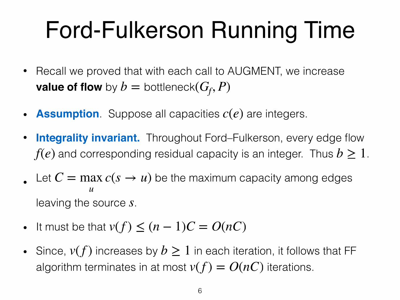
• Recall we proved that with each call to AUGMENT, we increase value of flow by

• Assumption. Suppose all capacities are integers.

• Integrality invariant. Throughout Ford–Fulkerson, every edge flow and corresponding residual capacity is an integer. Thus .

• Let be the maximum capacity among edges

leaving the source .

• It must be that

• Since, increases by in each iteration, it follows that FF algorithm terminates in at most iterations.

b = bottleneck(Gf , P)

c(e)

f(e) b ≥ 1

C = maxu

c(s → u)

s

v( f ) ≤ (n − 1)C = O(nC)

v( f ) b ≥ 1v( f ) = O(nC)

Ford-Fulkerson Running Time

6

• Claim. Ford-Fulkerson can be implemented to run in time , where and

.

• Proof. We know algorithm terminates in at most iterations. Each iteration takes time:

• We need to find an augmenting path in

• has at most edges, using BFS/DFS takes time

• Augmenting flow in takes time

• Given new flow, we can build new residual graph in time

O(nmC) m = |E | ≥ n − 1C = max

uc(s → u)

CO(m)

Gf

Gf 2mO(m + n) = O(m)

P O(n)

O(m) ∎

Ford-Fulkerson Running Time

7

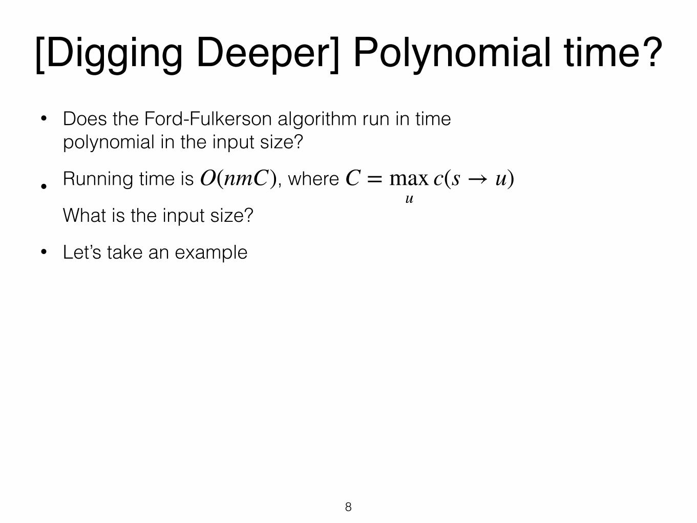
[Digging Deeper] Polynomial time?• Does the Ford-Fulkerson algorithm run in time

polynomial in the input size?

• Running time is , where

What is the input size?

• Let’s take an example

O(nmC) C = maxu

c(s → u)

8

• Question. Does the Ford-Fulkerson algorithm run in polynomial-time in the size of the input?

• Answer. No. if max capacity is , the algorithm can take iterations. Consider the following example.

C≥ C

9

1

C

C

C

C

t

s

v w

・s→v→w→t

・s→w→v→t

・s→v→w→t

・s→w→v→t

・…

・s→v→w→t

・s→w→v→t

each augmenting pathsends only 1 unit of flow

(# augmenting paths = 2C)

[Digging Deeper] Polynomial time?

~ m, n, and log C

[Digger Deeper] Pseudo-Polynomial• Input graph has nodes and edges, each

with capacity

• = , then takes bits to represent

• Input size: bits

• Running time: , exponential in the size of

• Such algorithms are called pseudo-polynomial

• If the running time is polynomial in the magnitude but not size of an input parameter.

• We saw this for knapsack as well!

n m = O(n2)ce

C maxe∈E

c(e) c(e) O(log C)

Ω(n log n + m log n + m log C)

O(nmC) = O(nm2log C)C

10

Non-Integral Capacities?

• If the capacities are rational, can just multiply to obtain a large integer (massively increases running time)

• If capacities are irrational, Ford-Fulkerson can run infinitely!

• Idea: amount of flow sent decreases by a constant factor each loop

Network Flow: Beyond Ford Fulkerson

12

Edmond and Karp’s Algorithms• Ford and Fulkerson’s algorithm does not specify which

path in the residual graph to augment

• Poor worst-case behavior of the algorithm can be blamed on bad choices on augmenting path

• Better choice of augmenting paths. In 1970s, Jack Edmonds and Richard Karp published two natural rules for choosing augmenting paths

• Fattest augmenting paths first

• Shortest (in terms of edges) augmenting paths first (Dinitz independently discovered & analyzed this rule)

• Can result in timeO(n2m)

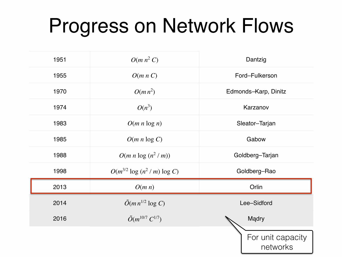
Progress on Network Flows1951 O(m n2 C) Dantzig

1955 O(m n C) Ford–Fulkerson

1970 O(m n2) Edmonds–Karp, Dinitz

1974 O(n3) Karzanov

1983 O(m n log n) Sleator–Tarjan

1985 O(m n log C) Gabow

1988 O(m n log (n2 / m)) Goldberg–Tarjan

1998 O(m3/2 log (n2 / m) log C) Goldberg–Rao

2013 O(m n) Orlin

2014 Õ(m n1/2 log C) Lee–Sidford

2016 Õ(m10/7 C1/7) Mądry

For unit capacity networks

Progress on Network Flows• Best known:

• Best lower bound?

• None known. (Needs just to look at the network, but that’s it)

• Some of these algorithms do REALLY well in “practice;” basically

• Well-known open problem

O(nm)

Ω(n + m)

O(n + m)

Applications of Network Flow: Solving Problems by

Reduction to Network Flows

16

Max-Flow Min-Cut Applications

• Data mining • Bipartite matching • Network reliability • Image segmentation • Baseball elimination • Network connectivity • Markov random fields • Distributed computing • Network intrusion detection • Many, many, more.

17

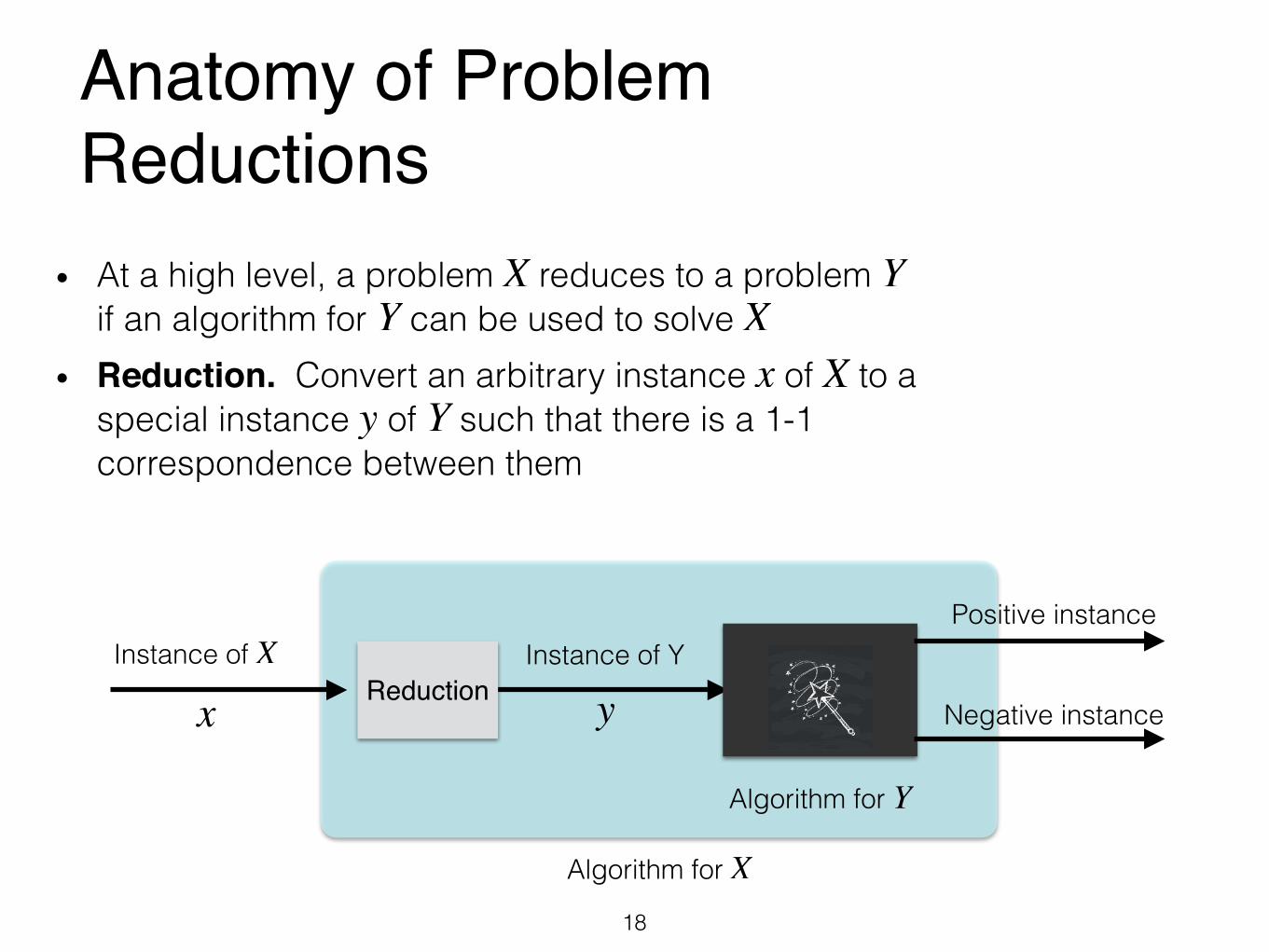
Anatomy of Problem Reductions

xInstance of X

yInstance of Y

Algorithm for Y

Positive instance

Negative instanceReduction

Algorithm for X

• At a high level, a problem reduces to a problem if an algorithm for can be used to solve

• Reduction. Convert an arbitrary instance of to a special instance of such that there is a 1-1 correspondence between them

X YY X

x Xy Y

18

Anatomy of Problem Reductions

• Claim. satisfies a property iff satisfies a corresponding property

• Proving a reduction is correct: prove both directions • has a property (e.g. has matching of size has a

corresponding property (e.g. has a flow of value • does not have a property (e.g. does not have matching of

size does not have a corresponding property (e.g. does not have a flow of value

• Or equivalently (and this is often easier to prove): • has a property (e.g. has flow of value has a

corresponding property (e.g. has a matching of value

x y

x k) ⟹ yk)

xk) ⟹ y

k)

y k) ⟹ xk)

19

Plan for Today

• I’ll show you one (classic) network flow reduction

• Then you’ll attempt one; we’ll go over the answer together

Max-Cardinality Bipartite Matching

21

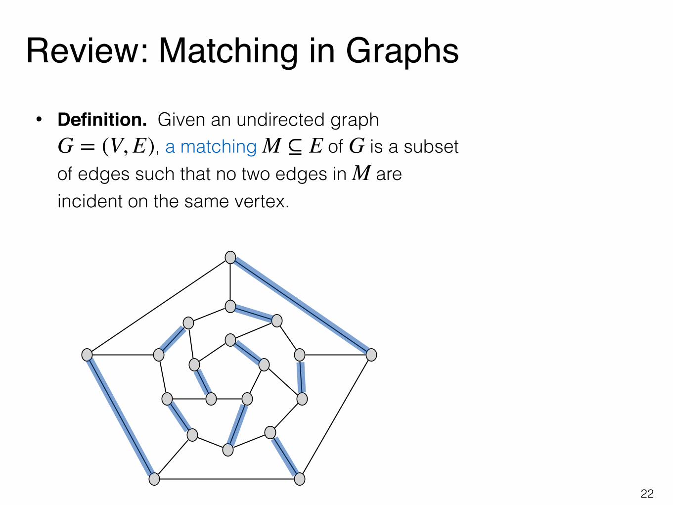
Review: Matching in Graphs• Definition. Given an undirected graph

, a matching of is a subset of edges such that no two edges in are incident on the same vertex.

G = (V, E) M ⊆ E GM

22

Review: Matching in Graphs• Definition. Given an undirected graph

, a matching of is a subset of edges such that no two edges in are incident on the same vertex.

• Max matching problem. Find a matching of maximum cardinality for a given graph, that is, a matching with maximum number of edges

G = (V, E) M ⊆ E GM

23

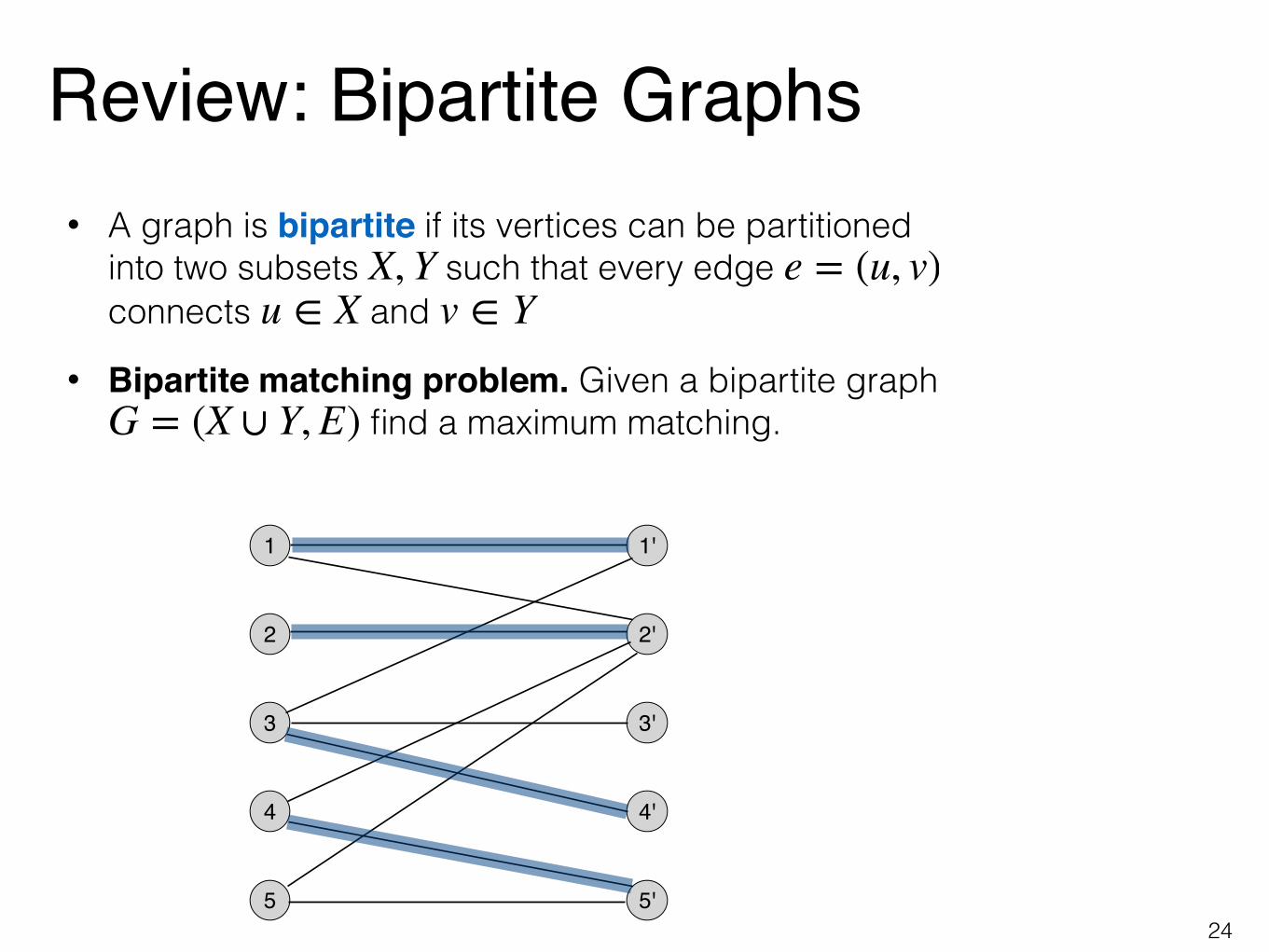
Review: Bipartite Graphs• A graph is bipartite if its vertices can be partitioned

into two subsets such that every edge connects and

• Bipartite matching problem. Given a bipartite graph find a maximum matching.

X, Y e = (u, v)u ∈ X v ∈ Y

G = (X ∪ Y, E)

1

2

3

4

5

1'

2'

3'

4'

5'24

Bipartite Matching Example• Suppose is a set of students, as a set of dorms

• Each student lists a set of dorms they’d like to live in, each dorm lists students it is willing to accommodate

• Goal. Find the largest matching (student, dorm) pairs that satisfies their requirements

• Bipartite matching instance. and if student and dorm are mutually acceptable, goal is to find maximum matching

• Note. This is a different problem than the one we studied for Gale-Shapely matching!

A B

V = (A, B) e ∈ E

25

Reduction to Max Flow

xInstance of X

yInstance of Y

Algorithm for Y

Positive instance

Negative instanceReduction

Algorithm for X

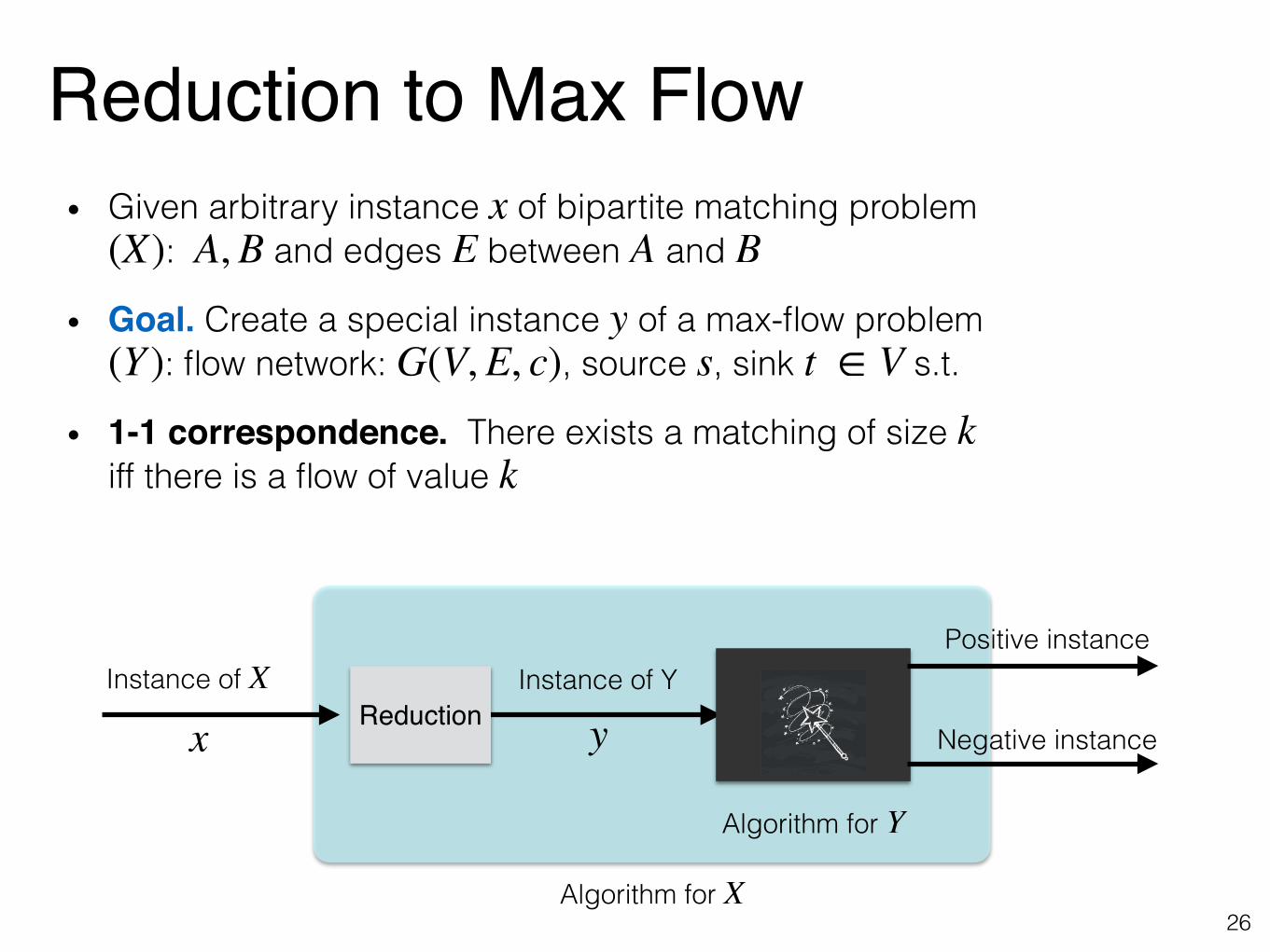
• Given arbitrary instance of bipartite matching problem : and edges between and

• Goal. Create a special instance of a max-flow problem : flow network: , source , sink s.t.

• 1-1 correspondence. There exists a matching of size iff there is a flow of value

x(X) A, B E A B

y(Y ) G(V, E, c) s t ∈ V

kk

26

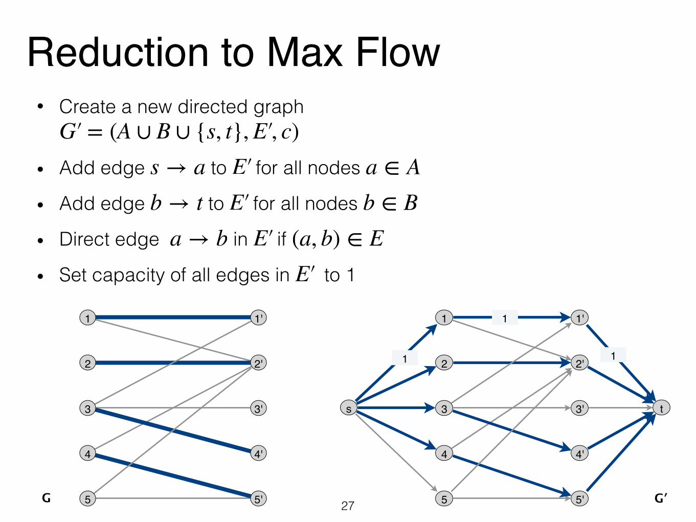
Reduction to Max Flow• Create a new directed graph

• Add edge to for all nodes

• Add edge to for all nodes

• Direct edge in if

• Set capacity of all edges in to 1

G′ = (A ∪ B ∪ {s, t}, E′ , c)s → a E′ a ∈ Ab → t E′ b ∈ B

a → b E′ (a, b) ∈ EE′

27

s

1

3

5

1'

3'

5'

t

2

4

2'

4'

1 1

G′

1

G

1

3

5

1'

3'

5'

2

4

2'

4'

Correctness of Reduction• Claim .

If the bipartite graph has matching of size then flow-network has an integral flow of value .

( ⇒ )(A, B, E) M k

G′ k

s

1

3

5

1'

3'

5'

t

2

4

2'

4'

1 1

G′

1

G

1

3

5

1'

3'

5'

2

4

2'

4'

28

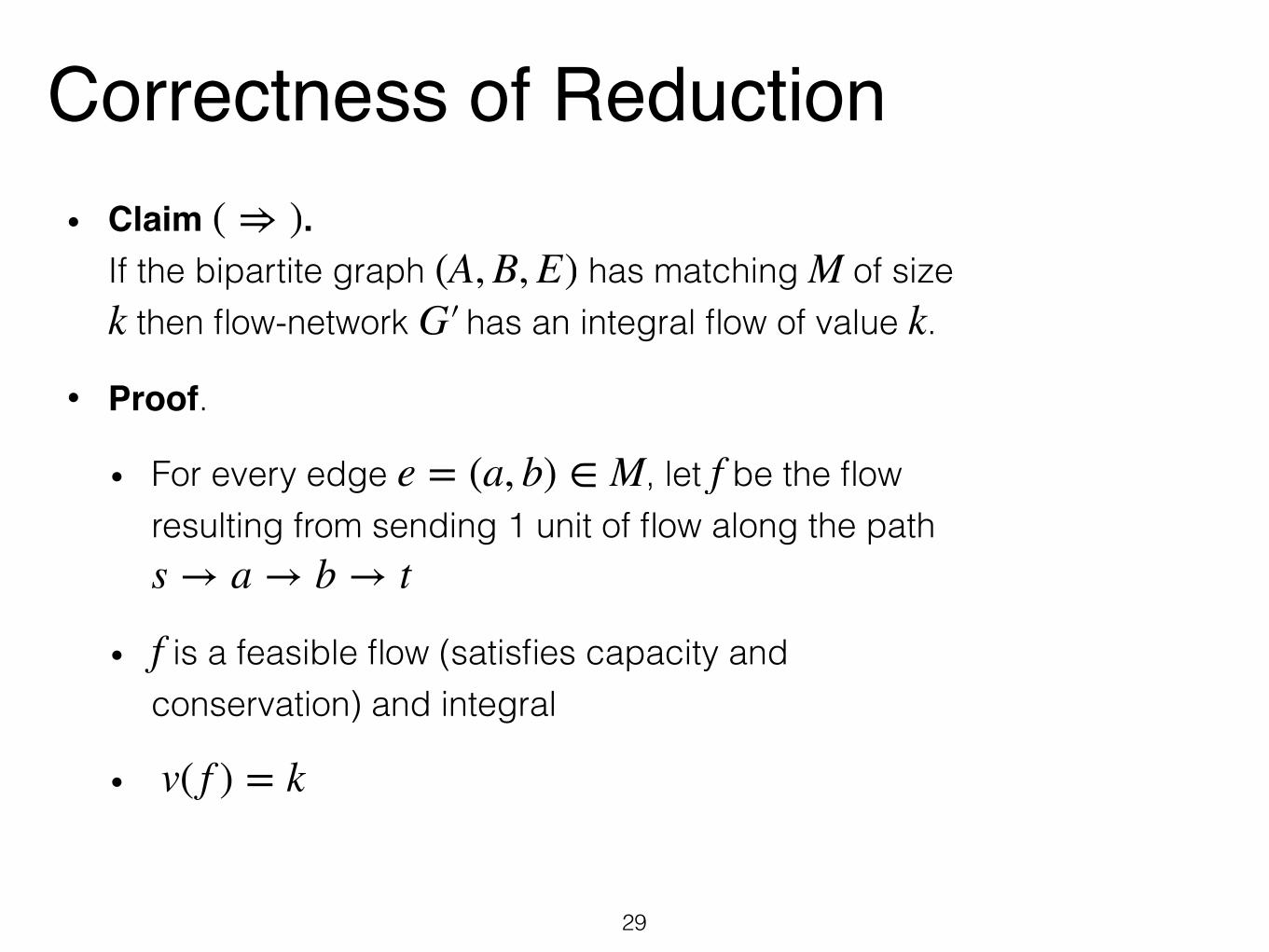
Correctness of Reduction• Claim .

If the bipartite graph has matching of size then flow-network has an integral flow of value .

• Proof.

• For every edge , let be the flow resulting from sending 1 unit of flow along the path

• is a feasible flow (satisfies capacity and conservation) and integral

•

( ⇒ )(A, B, E) M

k G′ k

e = (a, b) ∈ M f

s → a → b → t

f

v( f ) = k

29

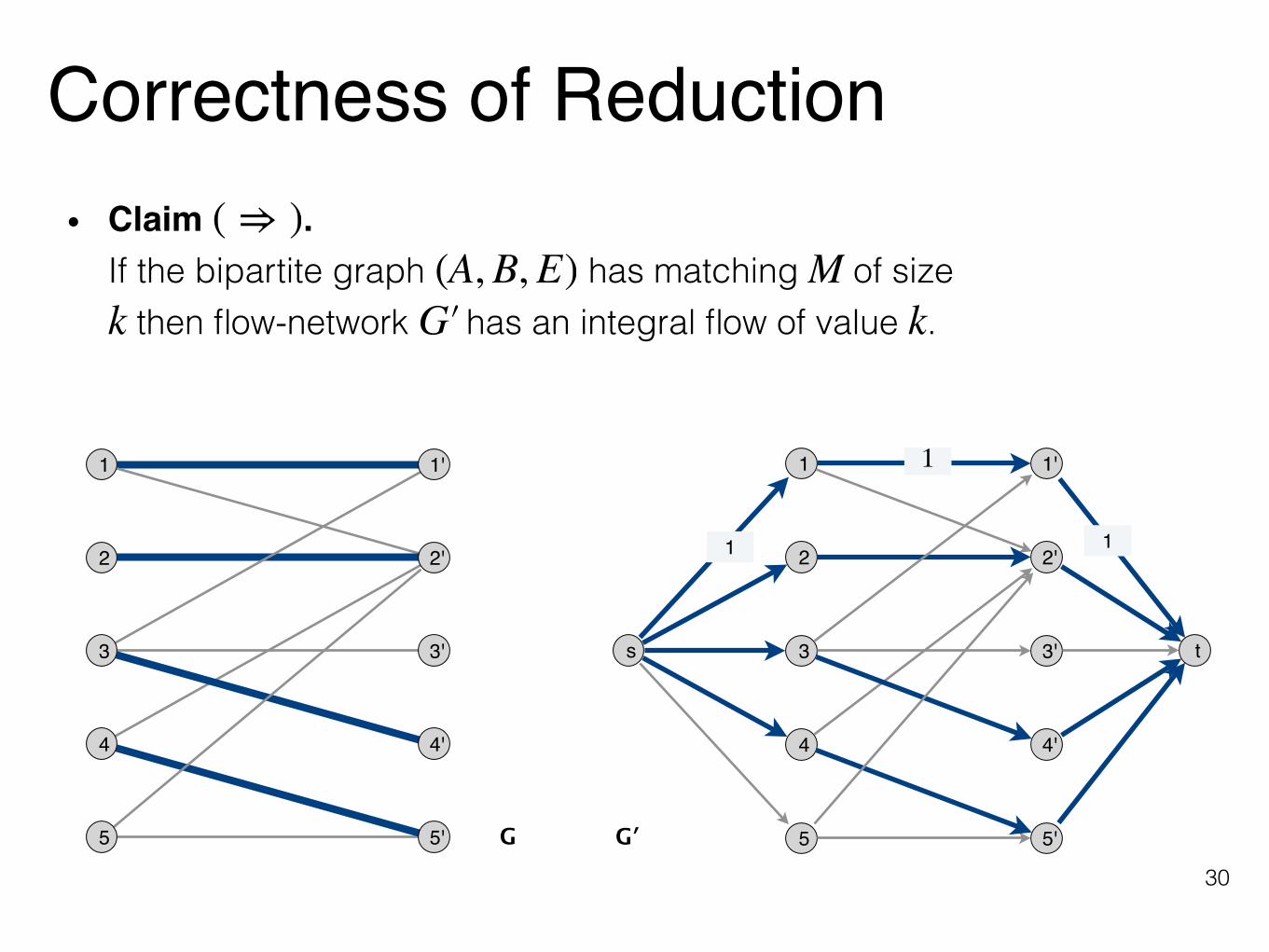
• Claim . If the bipartite graph has matching of size then flow-network has an integral flow of value .

( ⇒ )(A, B, E) M

k G′ k

s

1

3

5

1'

3'

5'

t

2

4

2'

4'

1 1

1

G′G

1

3

5

1'

3'

5'

2

4

2'

4'

Correctness of Reduction

30

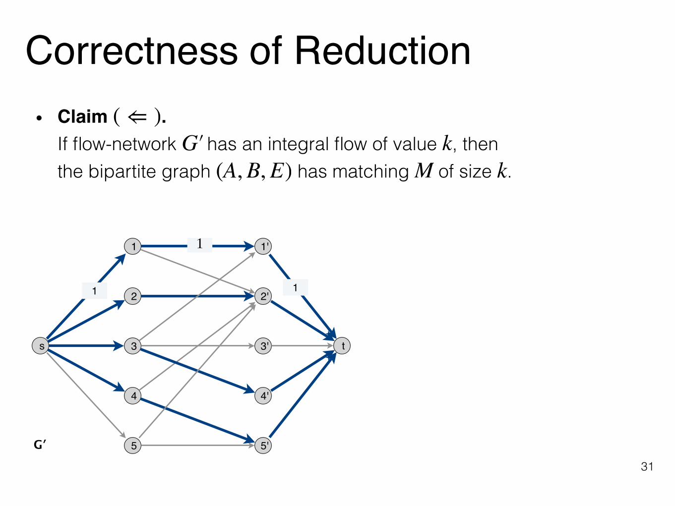
• Claim . If flow-network has an integral flow of value , then the bipartite graph has matching of size .

( ⇐ )G′ k

(A, B, E) M k

s

1

3

5

1'

3'

5'

t

2

4

2'

4'

1 1

1

G′

Correctness of Reduction

31

• Claim . If flow-network has an integral flow of value , then the bipartite graph has matching of size .

• Proof.

• Let set of edges from to with .

• No two edges in share a vertex, why?

•

• for any cut

• Let

( ⇐ )G′ k

(A, B, E) M k

M = A B f(e) = 1

M

|M | = k

v( f ) = fout(S) − fin(S) (S, V − S)

S = A ∪ {s}

Correctness of Reduction

32

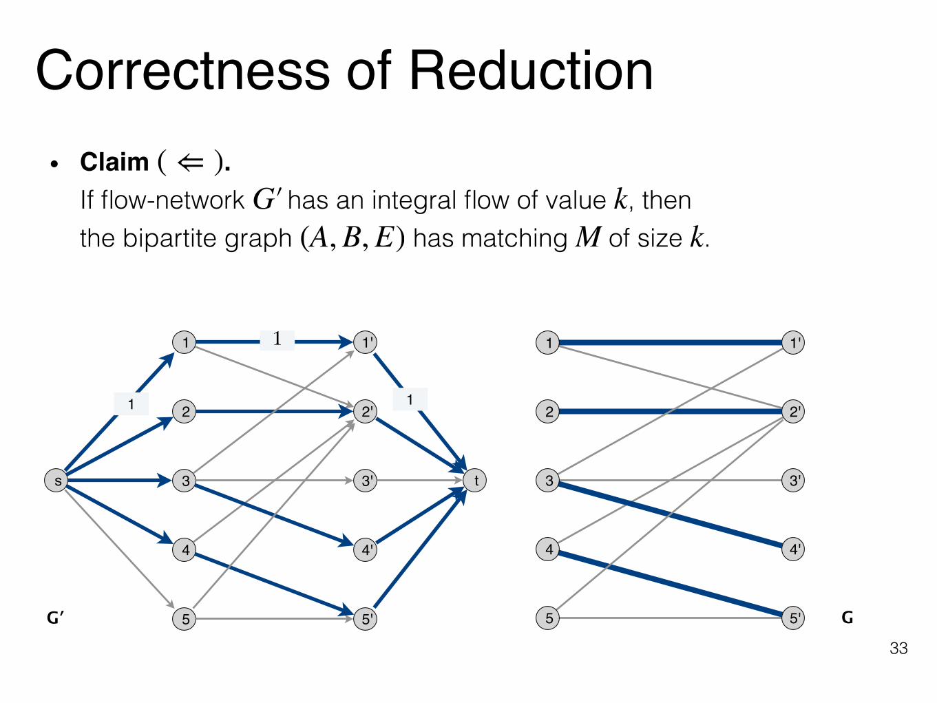
• Claim . If flow-network has an integral flow of value , then the bipartite graph has matching of size .

( ⇐ )G′ k

(A, B, E) M k

s

1

3

5

1'

3'

5'

t

2

4

2'

4'

1 1

1

G′ G

1

3

5

1'

3'

5'

2

4

2'

4'

Correctness of Reduction

33

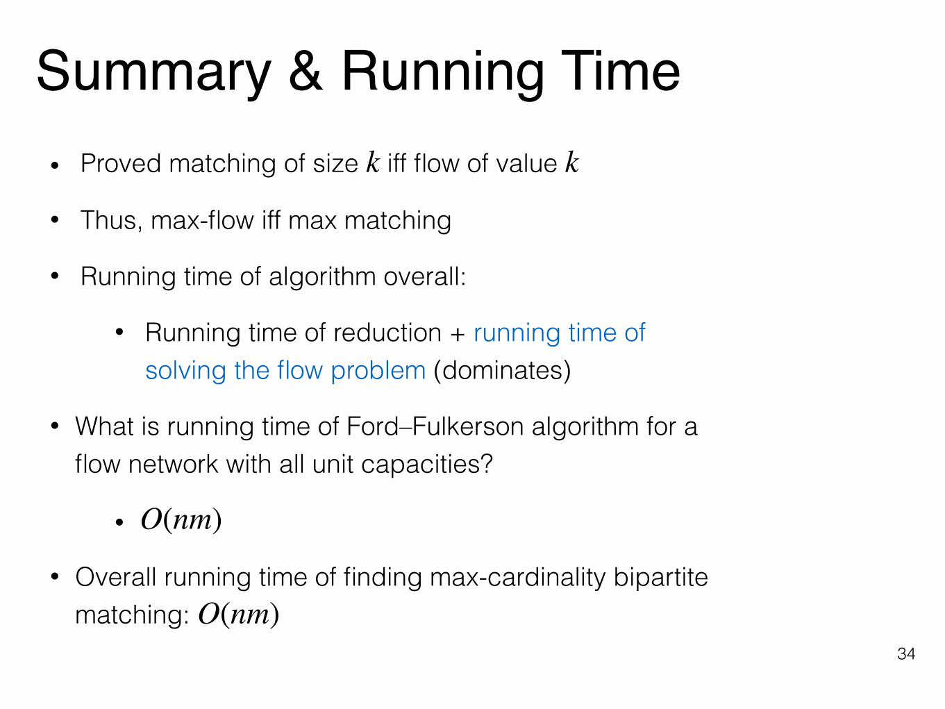
• Proved matching of size iff flow of value

• Thus, max-flow iff max matching

• Running time of algorithm overall:

• Running time of reduction + running time of solving the flow problem (dominates)

• What is running time of Ford–Fulkerson algorithm for a flow network with all unit capacities?

•

• Overall running time of finding max-cardinality bipartite matching:

k k

O(nm)

O(nm)

Summary & Running Time

34

Disjoint Paths Problem

35

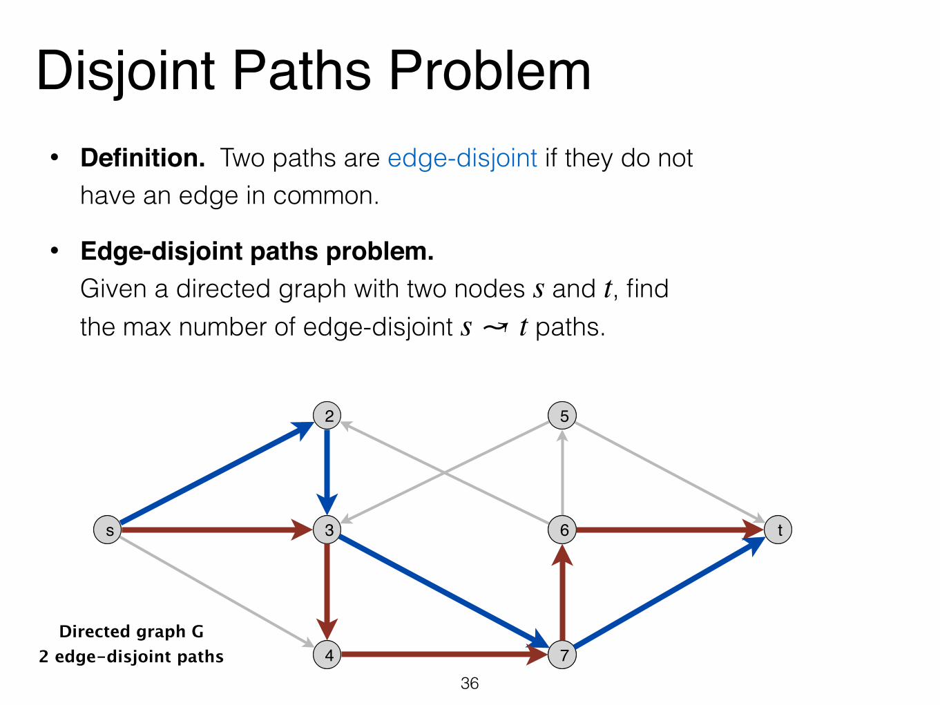
Disjoint Paths Problem• Definition. Two paths are edge-disjoint if they do not

have an edge in common.

• Edge-disjoint paths problem. Given a directed graph with two nodes and , find the max number of edge-disjoint paths.

s ts ↝ t

Directed graph G2 edge-disjoint paths

s

2

3

4

5

6

7

ts

2

3

4

5

6

7

t

36

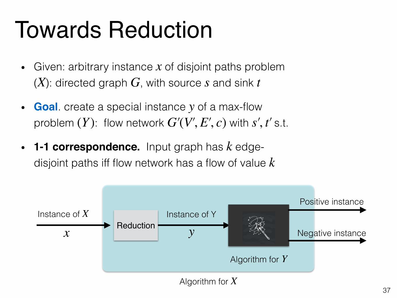
Towards Reduction• Given: arbitrary instance of disjoint paths problem

( ): directed graph , with source and sink

• Goal. create a special instance of a max-flow problem : flow network with s.t.

• 1-1 correspondence. Input graph has edge-disjoint paths iff flow network has a flow of value

xX G s t

y(Y ) G′ (V′ , E′ , c) s′ , t′

kk

xInstance of X

yInstance of Y

Algorithm for Y

Positive instance

Negative instanceReduction

Algorithm for X37

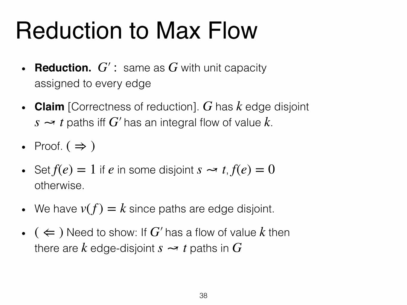
Reduction to Max Flow• Reduction. same as with unit capacity

assigned to every edge

• Claim [Correctness of reduction]. has edge disjoint paths iff has an integral flow of value .

• Proof.

• Set if in some disjoint , otherwise.

• We have since paths are edge disjoint.

• Need to show: If has a flow of value then there are edge-disjoint paths in

G′ : G

G ks ↝ t G′ k

( ⇒ )

f(e) = 1 e s ↝ t f(e) = 0

v( f ) = k

( ⇐ ) G′ kk s ↝ t G

38

Correction of Reduction• Claim. If is a 0-1 flow of value in , then the

set of edges where contains a set of edge-disjoint paths in .

• Proof [By induction on the # of edges with ]

• If , no edges carry flow, nothing to prove

• IH: Assume claim holds for all flows that use edges

• Consider an edge with

• By flow conservation, there exists an edge with , continue “tracing out the path" until

• Case (a) reach , Case (b) visit a vertex for a 2nd time

( ⇐ ) f k G′

f(e) = 1 ks ↝ t G

k′ f(e) = 1

k′ = 0

< k′

s → u f(s → u) = 1

u → vf(u → v) = 1

t v

39

Correction of Reduction• Case (a) We reach , then we found a path

• Decrease the flow on edges of by 1

•

• Number of edges that carry flow now : can apply IH and find other disjoint paths

• Case (b) visit a vertex for a 2nd time: consider cycle of edges visited btw 1st and 2nd visit to

• : decrease flow values on edges in to zero

• but # of edges in that carry flow , can now apply IH to get edge disjoint paths

t s ↝ t Pf′ : Pv( f′ ) = v( f ) − 1 = k − 1

< k′

k − 1 s ↝ tv

C vf′ Cv( f′ ) = v( f ) f′

< k′ k

∎

40

• Proved edge-disjoint paths iff flow of value

• Thus, max-flow iff max # of edge-disjoint paths

• Running time of algorithm overall:

• Running time of reduction + running time of solving the max-flow problem (dominates)

• What is running time of Ford–Fulkerson algorithm for a flow network with all unit capacities?

•

• Overall running time of finding max # of edge-disjoint paths:

k k

s ↝ t

O(nm)

s ↝ t O(nm)

Summary & Running Time

41

[Take-home Exercise] Reduction to Think About

42

Room Scheduling• Williams College is holding a big gala and has

hired you to write an algorithm to schedule rooms for all the different parties happening as part of it.

• There are parties and the th party has invitees.

• There are different rooms and the th room can fit people in it.

• Thus, party can be held in room iff .

• Describe and analyze an efficient algorithm to assign a room to each party (or report correctly that no such assignment is possible).

n i pi

r jrj

i j pi ≤ rj

43

Acknowledgments• Some of the material in these slides are taken from

• Kleinberg Tardos Slides by Kevin Wayne (https://www.cs.princeton.edu/~wayne/kleinberg-tardos/pdf/04GreedyAlgorithmsI.pdf)

• Jeff Erickson’s Algorithms Book (http://jeffe.cs.illinois.edu/teaching/algorithms/book/Algorithms-JeffE.pdf)