network by a PV generator with respect to voltage level ...

Investigations of the effects of supplying Jenin’s power distribution

network by a PV generator with respect to voltage level, power

losses, P.F and harmonics

By: Ibrahim Anwar Ibrahim

Ihsan Abd Alfattah Omareya

The supervisor: Dr. Maher Khammash

Outline:

Introduction

Problem Statement

Objectives

Scope

Methodology

Results and Analysis

Conclusion

Constraints

Recommendation

Introduction:

Due to the global trend toward the clean energy resources, it is very important to make our projects

and researches related with it. Moreover, we need to find the best solutions for improving our

power networks taking into consideration the best possible price which represented in the almost

free sources such as solar energy, especially that we are under the occupation and we don't have

control on our networks or the electricity generation.

The share of grid-connected photovoltaic (PV) power sources in power distribution systems is expected

to rise due to increasing costs of traditional fossil-fuel sources and continuous reduction of PV

generators worldwide. This project will present the schematic diagram of a complete PV generator with

control system (design with detailed specifications) to be connected safely with the electric network in

Jenin.

Problem Statement:

We will investigate what is the possibility of using PV generators in order to improve the action of

the system was selected from one part of Jenin’s power distribution network that contains 25 bus in the

same voltage level that consume 10.076 MW, 3.075 MVAR and total power losses 0.136 MW, 0.096

MVAR at Maximum load and consume 1.878 MW, 0.859 MVAR and total power losses 0.00538 MW,

0.00377 MVAR at Minimum load taking in consideration the voltage levels, power losses, P.F and

harmonics.

Objectives:

Find the optimal placement and sizing of distribution generation PV units in the network.

Study the impact of the added PV DG units by conducting a new power flow study and

harmonic distortion analysis.

Economic evaluation of the added PV DG units.

Methodology:

This study will be carried out on – Jenin's power distribution network-West Bank – Palestine. Some

information about the network and it's component specifications (like cables, transformers, loads, ...

etc) will be used. Also some specialized simulation software such as MATLAB, ETAP, and GIS are used to

analyze and study the above mentioned effects.

After analyzing the targeted network, we will review relevant research work in order to layout and

design an appropriate PV generator to be connected with the busses of Jenin network. After that we will

use simulation models to investigate the effect s of connecting PV generator with the outlined grid.

Through simulation technique, the effects of this PV on P.F, power losses, voltage level, harmonics and

reactive power flow in the network will be investigated. We expect that our work will yield an

improvement of power quality and distribution reliability of Jenin network by connecting of PV

generators.

Part 1:

From the literature reviews we found that the more suitable methodology to have optimal location and

sizing of DG in the system is one of Artificial Intelligent techniques called “Particle Swarm Optimization

(PSO)” because it is fast and accurate to find the optimum location and sizing of the photovoltaic

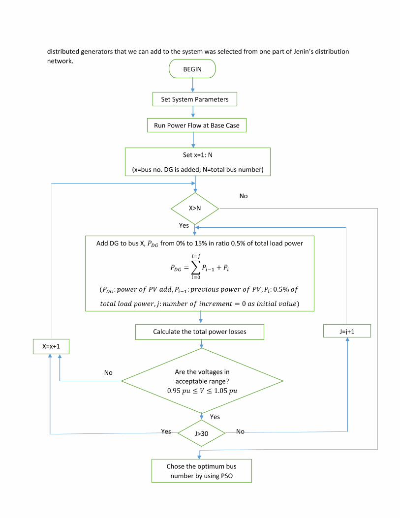
distributed generators that we can add to the system was selected from one part of Jenin’s distribution

network.

No

Yes

No

Yes

Yes No

BEGIN

Set System Parameters

Run Power Flow at Base Case

Set x=1: N

(x=bus no. DG is added; N=total bus number)

X>N

Add DG to bus X, 𝑃𝐷𝐺 from 0% to 15% in ratio 0.5% of total load power

𝑃𝐷𝐺 = ∑ 𝑃𝑖−1

𝑖=𝑗

𝑖=0

+ 𝑃𝑖

(𝑃𝐷𝐺: 𝑝𝑜𝑤𝑒𝑟 𝑜𝑓 𝑃𝑉 𝑎𝑑𝑑, 𝑃𝑖−1: 𝑝𝑟𝑒𝑣𝑖𝑜𝑢𝑠 𝑝𝑜𝑤𝑒𝑟 𝑜𝑓 𝑃𝑉, 𝑃𝑖: 0.5% 𝑜𝑓

𝑡𝑜𝑡𝑎𝑙 𝑙𝑜𝑎𝑑 𝑝𝑜𝑤𝑒𝑟, 𝑗: 𝑛𝑢𝑚𝑏𝑒𝑟 𝑜𝑓 𝑖𝑛𝑐𝑟𝑒𝑚𝑒𝑛𝑡 = 0 𝑎𝑠 𝑖𝑛𝑖𝑡𝑖𝑎𝑙 𝑣𝑎𝑙𝑢𝑒)

Calculate the total power losses

Are the voltages in

acceptable range?

0.95 𝑝𝑢 ≤ 𝑉 ≤ 1.05 𝑝𝑢

Chose the optimum bus

number by using PSO

J>30

X=x+1

J=j+1

Part 2:

After finding the optimal location and sizing of DG that will add to the system, we will study the effects

of PV DG added on the system such as; the voltage drop, total power losses, power losses between the

branches, P.F, buses voltages and harmonics.

Part 3:

This part for economic evaluation of the added DG PV on the system, it will contains the capital

cost of PV and the other equipment need, the saving money after reduce the total power losses

and power generation, total annual saving, the saving money while 20 years (PV life cycle) and

the payback period.

Results and Analysis:

Part 1:

As the first results in our methodology to investigate what is the possibility of using PV

generators in order to improve the action of the system was selected from one part of Jenin’s power

distribution network that contains 25 bus in the same voltage level taking in consideration the

voltage levels, power losses, P.F and harmonics is make run of load flow in maximum and

minimum loads for the system.

End

The system that contains 25 bus at the same Voltage levels

Load Flow by using MATLAB (Newton Raphson Method):

Month Power Factor Q Generation (MVAR) P Generation (MW) P loss (MW) Q loss (MVAR)

Jan 0.909 0.859 1.878 0.0054 0.0038

Feb 0.909 0.859 1.878 0.0054 0.0038

Mar 0.909 0.859 1.878 0.0054 0.0038

Apr 0.96 3.075 10.076 0.136 0.096

May 0.96 3.075 10.076 0.136 0.096

Jun 0.96 3.075 10.076 0.136 0.096

Jul 0.96 3.075 10.076 0.136 0.096

Aug 0.96 3.075 10.076 0.136 0.096

Sep 0.96 3.075 10.076 0.136 0.096

Oct 0.909 0.859 1.878 0.0054 0.0038

Nov 0.909 0.859 1.878 0.0054 0.0038

Dec 0.909 0.859 1.878 0.0054 0.0038

The yearly load curve for the Main Feeder

From this yearly load curve we found that the Average Power=5.977 MW, Max. Power=10.076 MW and

Load Factor= 59.32%

As we mentioned before the total DG PV added must not exceed 15% of the total load in both situation

(min. and max. load) for the main feeder. We saw that the max. load for this feeder in (April., May., Jun.,

Jul., Aug. and Sep.) months and the min. load for this feeder in (Jan., Feb., Mar., Oct., Nov. and Dec.)

months.

Solar Energy Parameters for Jenin:

The monthly average solar radiation that recorded by Energy Research Center in 2012 in Jenin

city as the following table:

Month Jan Feb Mar Apr May Jun Jul Aug Sep Oct Nov Dec

G(W/m2) 208.3 263.6 362.8 464.2 552.6 598.7 585.6 528.8 449.6 335.1 242.1 191.4 T (°C) 11.3 12.7 16.7 23.1 27.9 31.3 34.0 34.2 31.5 25.7 18.7 13.2 Tilt Angle 47 45 35 29 20 15 18 25 32.5 44 55 58.5

Table 6.1 Average monthly solar radiation for Jenin City [7].

Monthly Average Solar Radiation at Jenin City:

0

2

4

6

8

10

12

Jan Feb Mar Apr May Jun Jul Aug Sep Oct Nov Dec

P G

ener

atio

n (

MW

)

Month

P Generation (MW)

Average monthly solar radiation for Jenin City

Peak Sun Shine Hour 5.4 H.

The solar radiation and the temperature are changed during the year in Jenin City. So that mean the

energy that generated from the PV array depends on these terms, so to have the maximum efficiency

we will use tracking solar system by MPPT algorithm device to change the tilt angle 12 times per year.

The maximum demand in these months (April., May., Jun., Jul., Aug. and Sep.) is 10.076 MW and the

maximum demand in these months (Jan., Feb., Mar., Oct., Nov. and Dec.) is 1.878 MW, so if we said that

the DG PV will be 15% of the total load, we can see that the PV power needed in (April., May., Jun., Jul.,

Aug. and Sep.) is 1.5 MW from PV and the PV power needed in (Jan., Feb., Mar., Oct., Nov. and Dec.) is

0.2817 MW from PV.

However, we use PV module from SUNTECH com. Called (SuperPoly STP300 – 24/Vd) at STP (1000

(w/m²), 25 (⁰C) ) to have maximum efficiency, but the average yearly solar radiation about 400 (W/m²)

so we will use 3 MW PV when we need 1.5 MW, and 800 KW PV when we need 218.7 KW by using the

previous equations, we have the following that describe the power that generate from the DG PV field

during the year and the suitable tilt angle needed to achieve the max. efficiency for this field :

Month Jan Feb Mar Apr May Jun Jul Aug Sep Oct Nov Dec

G(W/m2) 208.3 263.6 362.8 464.2 552.6 598.7 585.6 528.8 449.6 335.1 242.1 191.4 T (°C) 11.3 12.7 16.7 23.1 27.9 31.3 34.0 34.2 31.5 25.7 18.7 13.2

208.3263.6

362.8

464.2

552.6598.7 585.6

528.8

449.6

335.1

242.1191.4

0

100

200

300

400

500

600

700


G (

W/M

²)

MONTH

Monthly Average Solar Radiation (W/m²)

Tilt Angle 47 45 35 29 20 15 18 25 32.5 44 55 58.5

P generation-

Max.(MW) 0.591 0.746 1.010 1.253 1.456 1.550 1.495 1.349 1.163 0.892 0.665 0.537

P generation-

Min. (MW) 0.158 0.199 0.269 0.334 0.388 0.413 0.399 0.360 0.310 0.238 0.177 0.143

PV Power

generation -

Used (MW)

0.158 0.199 0.269 1.253 1.456 1.550 1.495 1.349 1.163 0.238 0.177 0.143

The Real Power generated yearly from the Solar Field.

After we found the optimum sizing that will add to Ayash Feeder we will find the optimum location for

this DG PV field by using PSO algorithm. Firstly, we implement this size in the all buses in the feeder.

The PSO algorithm takes for each bus 6 values as an initial values for voltage profile, power factor, total

real power losses and total reactive power losses by using the following equations:

𝑉𝑘+1 = 𝜔 ∗ 𝑉𝑘 + 𝐶1 ∗ 𝑟2 ∗ (𝑃𝑏𝑒𝑠𝑡 − 𝑆𝑘) + 𝐶2 ∗ 𝑟1 ∗ (𝐺𝑏𝑒𝑠𝑡 − 𝑆𝑘)

𝑆𝑘+1 = 𝑉𝑘+1 + 𝑆𝑘

Where:

𝜔 is the weighting function is usually used as follows:

𝜔 = 𝜔𝑚𝑎𝑥 −𝜔𝑚𝑎𝑥 − 𝜔𝑚𝑖𝑛

𝐼𝑡𝑟𝑒𝑚𝑎𝑥𝐼𝑡𝑟𝑒

𝜔𝑚𝑎𝑥 𝑎𝑛𝑑 𝜔𝑚𝑖𝑛 ∶ Are the maximum and minimum weights, respectively.

Appropriate values for 𝜔𝑚𝑎𝑥 𝑎𝑛𝑑 𝜔𝑚𝑖𝑛 are 0.4 and 0.9 [3]. The weights for each factor as the following:

Voltage profile: 50%

Power factor: 30%

Total real power losses: 10%

Total reactive power losses: 10%

The results as the following for maximum and minimum loads as the following:

Maximum load case:

# Bus Voltages P.F Total P loss Total Q loss

12 25 3 0.09417 0.066817

16 20 2 0.094383 0.066646

18 20 2 0.0944 0.066655

13 15 3 0.09431 0.066902

15 16 2 0.094709 0.06683

11 13 4 0.094734

PSO Bus selection in max. load.

As the above table shown the optimum location in max. load is bus #12.

Minimum load case:

# Bus Voltages P.F Total P loss Total Q loss

12 24 8 0.003887656 0.002744823

13 14 7 0.00388864 0.002745419

14 13 6 0.003911429 0.0027532

15 12 5 0.00391135 0.002751781

16 18 15 0.003910106 0.002745546

18 18 7 0.003908988 0.002744918

PSO Bus selection in min. load.

As the above table shown the optimum location in min. load is bus #12.

To sum up, we can notice that bus #12 is the optimum location in the both situation.

Part 2:

Discussion:

As we mentioned in the previous chapter that the optimum sizing was 1.5 MW in max. load and 218.7 KW in min. load and the optimum location was bus #12, the effects for this adding on the main

feeder as the following:

Month

Solar

Radiation

(W/m²)

Voltage

Profile

(P.U)

Total

Power

Factor

P

Generation

(MW)

P PV

(MW)

Q Generation

(MVAR)

Total P Loss

(MW)

Total Q

Loss(MW)

Jan 208.3 0.9965 0.895 1.72 0.158 0.859 0.005 0.003

Feb 263.6 0.9966 0.89 1.678 0.199 0.859 0.004 0.003

Mar 362.8 0.9968 0.882 1.608 0.269 0.858 0.004 0.003

Apr 464.2 0.9848 0.945 10.04 1.253 3.049 0.1001 0.071

May 552.6 0.9853 0.942 10.035 1.456 3.045 0.095 0.068

Jun 598.7 0.9856 0.941 10.033 1.55 3.044 0.093 0.066

Jul 585.6 0.9854 0.942 10.034 1.495 3.045 0.094 0.067

Aug 528.8 0.985 0.944 10.038 1.349 3.047 0.098 0.069

Table 8.1 The effects of add DG PV on bus 12

The power factor at the main feeder (Ayash Feeder) after add DG PV as the following fig. 8.1:

Fig 8.1 The power factor at the main feeder after add DG PV on bus 12

The total real power feed the all over main feeder (Ayash Feeder) after add DG PV as the following fig.

8.2:

0.8950.89

0.882

0.945 0.942 0.941 0.942 0.944 0.946

0.8860.893 0.896

0.84

0.86

0.88

0.9

0.92

0.94

0.96


P.F

MONTH

Ayash Feeder Power Factor

Sep 449.6 0.9845 0.946 10.042 1.163 3.05 0.102 0.073

Oct 335.1 0.9967 0.886 1.639 0.238 0.858 0.004 0.003

Nov 242.1 0.9966 0.893 1.7 0.177 0.859 0.004 0.003

Dec 191.4 0.9965 0.896 1.734 0.143 0.859 0.005 0.003

Fig 8.2 The total real power feed the all over main feeder after add DG PV on bus 12

Average Power=6.6459 MW, Max. Power=10.042 MW, Load Factor=66.18 %

The total Reactive power feed the all over main feeder (Ayash Feeder) after add DG PV as the following

fig. 8.3:

Fig 8.3 The total reactive power feed the all over main feeder after add DG PV on bus 12

The total real power and reactive power loss for the all over main feeder (Ayash Feeder) after add DG PV

as the following fig. 8.4:


P PV (MW) 0.158 0.199 0.269 1.253 1.456 1.55 1.495 1.349 1.163 0.238 0.177 0.143

P Generation (MW) 1.72 1.678 1.608 10.04 10.035 10.033 10.034 10.038 10.042 1.639 1.7 1.734

0

2

4

6

8

10

12

14

P G

ener

atio

n (

MW

)

Total Real Power Generation (MW)

P Generation (MW) P PV (MW)

0.859 0.859 0.858

3.049 3.045 3.044 3.045 3.047 3.05

0.858 0.859 0.859

0

0.5

1

1.5

2

2.5

3

3.5


Q G

ENER

ATI

ON

(M

VA

R)

MONTH

Total Reacive Power Generation (MVAR)

Fig 8.4 The total real power and reactive power loss for all over main feeder after add DG PV on bus 12

We can notice from the previous results that:

The power factor at the main feeder sharp decrease

The voltage profile at the main feeder gradual increase

The reactive power generation constant

The real power came from connection point steady decrease

The total real and reactive power losses within the system decrease

The load factor increase to become 66.18% from 59.32%

But, the effects on bus #12 as the following figures, we can noticed that the power factor

become unity and steady at 1, on the other hand the voltage profile sharp increased during the

year:


Total P Loss (MW) 0.005 0.004 0.004 0.1001 0.095 0.093 0.094 0.098 0.102 0.004 0.004 0.005

Total Q Loss(MW) 0.003 0.003 0.003 0.071 0.068 0.066 0.067 0.069 0.073 0.003 0.003 0.003

0

0.02

0.04

0.06

0.08

0.1

0.12

Total Losses

Total P Loss (MW) Total Q Loss(MW)

The voltage profile for bus #12 after add DG PV as the following fig. 8.5:

Fig 8.5 The voltage profile for bus #12 after add DG PV

The power factor at bus #12 after add DG PV as the following fig. 8.6:

Fig 8.6 The power factor at bus #12 after add DG PV

Although, we studied the effects that appear in the all buses when we add DG PV on bus #12,

the effects was the following figures and tables:

0.99650.99660.9968

0.98480.98530.98560.9854 0.985 0.9845

0.99670.99660.9965

0.978

0.98

0.982

0.984

0.986

0.988

0.99

0.992

0.994

0.996

0.998


V (

P.U

)

MONTH

Voltage Profile (P.U)

1 1 1 1 1 1 1 1 1 1 1 1

0

0.2

0.4

0.6

0.8

1

1.2


P.F

MONTH

Power Factor bus #12

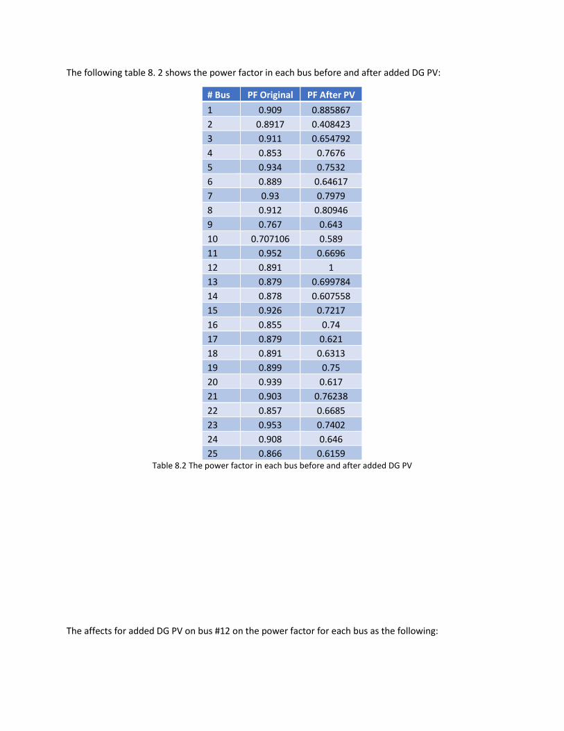
The following table 8. 2 shows the power factor in each bus before and after added DG PV:

# Bus PF Original PF After PV

1 0.909 0.885867

2 0.8917 0.408423

3 0.911 0.654792

4 0.853 0.7676

5 0.934 0.7532

6 0.889 0.64617

7 0.93 0.7979

8 0.912 0.80946

9 0.767 0.643

10 0.707106 0.589

11 0.952 0.6696

12 0.891 1

13 0.879 0.699784

14 0.878 0.607558

15 0.926 0.7217

16 0.855 0.74

17 0.879 0.621

18 0.891 0.6313

19 0.899 0.75

20 0.939 0.617

21 0.903 0.76238

22 0.857 0.6685

23 0.953 0.7402

24 0.908 0.646

25 0.866 0.6159 Table 8.2 The power factor in each bus before and after added DG PV

The affects for added DG PV on bus #12 on the power factor for each bus as the following:

Fig 8.7 The affects for added DG PV on bus #12 on the power factor for each bus

The following table shows the Voltage profile in each bus before and after added DG PV:

# Bus V original V after PV

1 1 1

2 0.98889624 0.989987

3 0.98886 0.989765

4 0.98575 0.9872

5 0.98597 0.9875

6 0.985 0.98703

7 0.9848 0.986571

8 0.9835532 0.98567

9 0.9827 0.985091

10 0.9819987 0.98459

11 0.981849 0.984533

12 0.98122843 0.984512

13 0.98099 0.984278

14 0.98093 0.984217

15 0.98177123 0.984363

16 0.98127757 0.98387

17 0.98117745 0.98377

18 0.9811353 0.983728

19 0.98093 0.983524

20 0.9887876 0.9899

21 0.9885 0.98964

22 0.988 0.98957

23 0.9883 0.989393

0

0.2

0.4

0.6

0.8

1

1.2

1 2 3 4 5 6 7 8 9 10 11 12 13 14 15 16 17 18 19 20 21 22 23 24 25

Po

wer

Fac

tor

Buses

Power Factor For Each Bus

PF Original PF After PV

24 0.9821263 0.989304

25 0.98820786 0.989299665 Table 8.3 The Voltage profile in each bus before and after added DG PV

The affects for added DG PV on bus #12 on the voltage profile for each bus as the following:

Fig 8.8 The affects for added DG PV on bus #12 on the voltage profile for each bus

The following table shows the total harmonic distortion (THD) in each bus before and after added DG PV

to bus #12:

0.97

0.975

0.98

0.985

0.99

0.995

1

1.005

1 2 3 4 5 6 7 8 9 10 11 12 13 14 15 16 17 18 19 20 21 22 23 24 25

V (

P.U

)

Bus Number

Voltage Profile For Each Bus

V original V after PV

Bus Num.

Voltage harmonic Before (%)

Voltage harmonic After (%)

Current harmonic Before (%)

Current harmonic After (%)

1 5.42 2.6 11.94 6.32

2 5.32 2.45 11.67 6.8

3 6.85 4.2 8.66 4.6

4 5.26 3.2 11.65 6.3

5 6.35 3.85 7.43 3.5

6 6.22 3.8 10.68 5.02

7 6.96 4.3 7.35 3.4

8 5.62 2.55 10.67 5.01

9 5.36 2.35 9.85 4.8

10 5.68 2.45 10.67 5.1

11 6.52 1.98 7.45 3.6

12 6.35 2.7 7.41 3.8

13 5.59 2.89 10.68 4.89

14 4.99 2.12 11.94 4.52

Table 8.4 The total harmonic distortion (THD) in each bus before and after added DG PV to bus #12

The Voltage Harmonic emission in the network after add DG PV to the bus #12 and how it effects on the

THD as the following:

Fig. 8.9 The Voltage Harmonic emission in the network after add DG PV to the bus #12

The Current Harmonic emission in the network after add DG PV to the bus #12 and how it effects on the

THD as the following:

0

1

2

3

4

5

6

7

8

1 2 3 4 5 6 7 8 9 10 11 12 13 14 15 16 17 18 19 20 21 22 23 24 25

V T

HD

(%

)

Bus Number

Voltage Harmonic

Voltage harmonic Before (%) Voltage harmonic After (%)

15 5.26 3.2 9.54 4.98

16 6.53 2 8.56 4.6

17 5.33 2.3 9.53 4.88

18 6.43 2.82 7.42 3.89

19 6.42 2.86 8.52 4.99

20 5.95 2.15 9.53 4.62

21 5.69 2.23 10.69 5.08

22 5.2 3.1 11.68 6.2

23 5.36 3.21 10.66 5.6

24 4.98 2.5 9.53 4.9

25 5.96 2.3 10.68 5.6

Fig. 8.10 The Current Harmonic emission in the network after add DG PV to the bus #12

We can notice from the previous results:

The power factor at each bus sharp decrease

The Voltage profile increase

The total losses decrease

The THD decrease for voltage and current signal

Part 3:

the one line diagram for An-Najah solar field that will feed Ayash feeder:

0

2

4

6

8

10

12

14

1 2 3 4 5 6 7 8 9 10 11 12 13 14 15 16 17 18 19 20 21 22 23 24 25

I TH

D (

%)

Bus Number

Current Harmonic

Current harmonic Before (%) Current harmonic After (%)

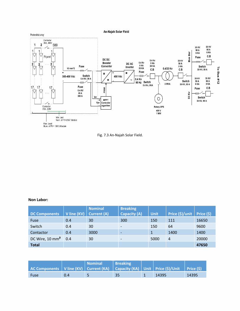
Fig. 7.3 An-Najah Solar Field.

Non Labor:

DC Components V line (KV) Nominal Current (A)

Breaking Capacity (A) Unit Price ($)/unit Price ($)

Fuse 0.4 30 300 150 111 16650

Switch 0.4 30 - 150 64 9600

Contactor 0.4 3000 - 1 1400 1400

DC Wire, 10 mm² 0.4 30 - 5000 4 20000

Total 47650

AC Components V line (KV) Nominal Current (KA)

Breaking Capacity (KA) Unit Price ($)/Unit Price ($)

Fuse 0.4 5 35 1 14395 14395

Table 7.15 DC Components, properties, units and price [12]

Table 7.16 AC Components, properties, units and price [12]

Table 7.17 other Components, properties, units and price [8,11,12,13]

Assets Area $/Year Year Price ($)

Site 20 Dunam 75000 20 1500000 Table 7.18 Assets, properties, duration and price

DC Components 47650 $

AC Components 229605 $

Other Components 2788852 $

Site 1500000 $

Switch 0.4 5 - 1 7500 7500

C.B, SF6 0.4 5 35 1 18710 18710

C.B, SF6 33 0.05 3 1 29000 29000

Fuse 33 0.05 3 2 23000 46000

Switch 33 0.05 - 2 24500 49000

C.B, SF6 33 0.05 6 2 30000 60000

Bas Bur 33 0.1 - 1 5000 5000

Total 229605

Other Components Properties Unit Price ($)/Unit Price ($)

PV Module_SUNTECH 300W/24Vd 10013 250 2503250

Transformer_Schneider 0.4/33 KV , 3MVA 1 30000 30000

DC/DC Converter_ SMA (300-400)V =400 V, 20000 W 150 500 75000

DC/AC Inverter _SMA 400 V = 400 V,50 Hz, 20000 W 150 1000 150000

Capacitor Banks_ABB 20KVAR, 400V 2 185 370



MPPT_SMA 150 100 15000

Motor 3 ph, 400 V, 10 Khp 1 10000 10000

Rotary UPS 400 V, 9 KAH 1 65000 65000

Total 2853852

Total ($) 4541107 $ Table 7.19 Total Non-labor resource Cost.

Labor:

Person Num. $/Hour Hours/ 18 Months Price ($)

Engineers 7 45 4320 194400

Technicians 20 23 4320 99360

Others 10 15 5000 75000

Total ($) 368760 $ Table 7.20 Total labor resource Cost.

Labor 368760 ($)

Non Labor 4631107 ($)

Currency Diffusion 133 ($)

Total Budget ($) 5000000 ($) Table 7.21 Total Capital Cost.

The annual saving for Ayash Feeder:

Original:

The annual max demand:

Pmax= 10.076 MW

Since the load factor (L.F) = 59.32 %

𝑃𝑎𝑣𝑔 = 𝐿. 𝐹 ∗ 𝑃𝑚𝑎𝑥

𝑃𝑎𝑣𝑔 = 0.5932 ∗ 10.076 ∗ 103 = 5977 𝐾𝑊

𝐸𝑛𝑒𝑟𝑔𝑦 (𝐸) = 𝑃𝑎𝑣𝑔 ∗ 8760 = 52359249 𝐾𝑊𝐻 𝑦𝑒𝑎𝑟𝑙𝑦

The cost per KWH is 0.62 NIS/KWH:

𝑇𝑜𝑡𝑎𝑙 𝑏𝑖𝑙𝑙 = 𝐸 ∗ 0.62 𝑁𝐼𝑆 𝐾𝑊𝐻⁄ = 32462734 𝑁𝐼𝑆 𝑝𝑒𝑟 𝑦𝑒𝑎𝑟

Since the power factor during the minimum load period less than 0.92 so the company is paying a

penalty as explained below:

𝐸𝑛𝑒𝑟𝑔𝑦/𝑚𝑜𝑛𝑡ℎ = 𝑃𝑎𝑣𝑔 ∗ 8760/12 = 4363271 𝐾𝑊𝐻 𝑚𝑜𝑛𝑡ℎ𝑙𝑦

𝑐𝑜𝑠𝑡 𝑝𝑒𝑟 𝑚𝑜𝑛𝑡ℎ = 2705228 𝑁𝐼𝑆 𝑝𝑒𝑟 𝑚𝑜𝑛𝑡ℎ

During the six month of minimum load the power factor =0.909

In Palestine the penalty for 0.8 ≤ 𝑝. 𝑓 ≤ 0.92 is 1% at total bill for each 0.1 under 0.92

0.92-0.909=0.011

𝑃𝑒𝑛𝑎𝑙𝑡𝑦 𝑝𝑒𝑟 𝑚𝑜𝑛𝑡ℎ = 0.011 ∗ 𝑇𝑜𝑡𝑎𝑙 𝑚𝑜𝑛𝑡ℎ𝑙𝑦 𝐵𝑖𝑙𝑙

𝑃𝑒𝑛𝑎𝑙𝑡𝑦 𝑝𝑒𝑟 𝑚𝑜𝑛𝑡ℎ = 0.011 ∗ 2705228

= 29758 𝑁𝐼𝑆 𝑝𝑒𝑟 𝑚𝑜𝑛𝑡ℎ

For the six months:

𝑇𝑜𝑡𝑎𝑙 𝑃𝑒𝑛𝑎𝑙𝑡𝑦 = 6 ∗ 29758 = 178548 𝑁𝐼𝑆

The total cost:

𝑇𝑜𝑡𝑎𝑙 𝑎𝑛𝑛𝑢𝑎𝑙 𝑐𝑜𝑠𝑡 = 𝐸𝑛𝑒𝑟𝑔𝑦 𝑐𝑜𝑠𝑡 + 𝑡𝑜𝑡𝑎𝑙 𝑝𝑒𝑛𝑎𝑙𝑡𝑦

= 32462734 + 178548

= 32641282 𝑁𝐼𝑆

= 𝟗𝟒𝟎𝟔𝟕𝟏𝟎 $ .

After using DG PV:

The annual max demand:

Pmax= 8.879 MW

Since the load factor (L.F) = 66.18 %

𝑃𝑎𝑣𝑔 = 𝐿. 𝐹 ∗ 𝑃𝑚𝑎𝑥

𝑃𝑎𝑣𝑔 = 0.6618 ∗ 8.879 ∗ 103 = 5070.92 𝐾𝑊

𝑃𝑎𝑣𝑔 = 5070.92 𝐾𝑊

𝐸𝑛𝑒𝑟𝑔𝑦 (𝐸) = 𝑃𝑎𝑣𝑔 ∗ 8760 = 44421259 𝐾𝑊𝐻 𝑦𝑒𝑎𝑟𝑙𝑦

The cost per KWH is 0.62 NIS/KWH

𝑇𝑜𝑡𝑎𝑙 𝑏𝑖𝑙𝑙 = 𝐸 ∗ 0.62 𝑁𝐼𝑆 𝐾𝑊𝐻⁄ = 27541181 𝑁𝐼𝑆 𝑝𝑒𝑟 𝑦𝑒𝑎𝑟

Before using PV After using PV

Total annual cost 32641282 NIS 27541181 NIS

Cost in $ (1$=3.47 NIS) 9406710 $ 7936940 $ Table 7.22 Total annual Cost before and after add DG PV.

𝑇ℎ𝑒 𝑦𝑒𝑎𝑟𝑙𝑦 𝑠𝑎𝑣𝑖𝑛𝑔 = 9406710 − 7936940

= 𝟏𝟒𝟔𝟗𝟕𝟕𝟎 $

The Payback Period:

𝑃. 𝐵. 𝑃 =𝐶𝑎𝑝𝑖𝑡𝑎𝑙 𝐶𝑜𝑠𝑡

𝑆𝑎𝑣𝑖𝑛𝑔

𝑃. 𝐵. 𝑃 =5000000 $

1469770 $

𝑃. 𝐵. 𝑃 = 3.5 𝑌𝑒𝑎𝑟

By the way the life cycle of the equipment in the solar field is about 20 Year and the payback

period is 3.5 Year, so the total saving after 3.5 years of implemented this project will be

𝑆𝑎𝑣𝑖𝑛𝑔 𝑎𝑓𝑡𝑒𝑟 3.5 𝑌𝑒𝑎𝑟 = (20 − 3.5) ∗ 𝑌𝑒𝑎𝑟𝑙𝑦 𝑆𝑎𝑣𝑖𝑛𝑔

𝑆𝑎𝑣𝑖𝑛𝑔 𝑎𝑓𝑡𝑒𝑟 3.5 𝑌𝑒𝑎𝑟 = 16.5 ∗ 1469770

𝑆𝑎𝑣𝑖𝑛𝑔 𝑎𝑓𝑡𝑒𝑟 3.5 𝑌𝑒𝑎𝑟 = 𝟐𝟒𝟐𝟓𝟏𝟐𝟎𝟓 $

To sum up, one can show that the project is feasible to implement.

Conclusions and Recommendation:

In general, we can conclude that this project will be a strong solution for this problem due to

the improvement that happened after add DG PV on this feeder in Jenin City, especially in bus

#12.

To sum up, the all effects on the system after add DG PV as the following:

The voltage profile increase within the range (1.05≤ V ≤ 0.95) that can increase the

efficiency of the supply from one hand, so the current in the system will decrease that

mean the total losses will decrease, so the total bill will decrease, from the other hand

we can use the same feeder to add new load within range that did not let the voltage be

less than 0.95 P.U, so we can make a long term control without need new transformers.

The total harmonic distortion in the system will decrease it can be seen that only the 12th, 15th, 18th, 21st and 24th harmonics exceeded the threshold limits. However, total voltage harmonics distortion for all of the studied cases is within the Australian regulatory standard limit as stated in AS 4777 [10], total Harmonic Distortion gives us the information about the harmonic content in a signal w.r.t. fundamental component, so that mean increase the power quality for the supply.

The total real and reactive power losses decrease sharply, due to increase the voltage

profile and decrease the currents in the system in the same time.

The total saving in the total bill will be about 24 Million $.

The only bad effect for this solution was decrease the power factor in the system, so

that mean the penalty will be huge, so we recommend to use capacitor banks to

increase the power factor to be equal or more than 92%.

The recommendation to improve power factor is to use capacitor banks as the following:

# Bus PF Original PF After PV Capacitor Bank (KVAR)

1 0.909 0.885867 20

2 0.8917 0.408423 30

3 0.911 0.654792 30

4 0.853 0.7676 25

5 0.934 0.7532 30

6 0.889 0.64617 25

7 0.93 0.7979 25

8 0.912 0.80946 20

9 0.767 0.643 30

10 0.707106 0.589 30

11 0.952 0.6696 25

12 0.891 1 0

13 0.879 0.699784 25

14 0.878 0.607558 30

15 0.926 0.7217 25

16 0.855 0.74 25

17 0.879 0.621 30

18 0.891 0.6313 30

19 0.899 0.75 25

20 0.939 0.617 30

21 0.903 0.76238 25

22 0.857 0.6685 30

23 0.953 0.7402 25

24 0.908 0.646 30

25 0.866 0.6159 30 Table 9.1 Improve power factor and the value of capacitor banks

By using the above values of capacitor banks that will increase the power factor to be at least

92%, on the other hand will increase the voltage at the bus but within the voltage rang.

Constraints:

As any problem in our life we will find the suitable solution for it in many terms to solve it from one side and to have the stability for this solution during a long term period, so in this case we will use SMART method to solve it. SMART method means that the solution will be specific, measurable, achievable, realistic and have time frame to have long term solution for any problem. So to satisfy this method we faced many constraints and the constraints in our project can be divided into four parts: 1. Leakage in Data base from the supplier.

2. Unrealistic solution for this problem.

3. No Palestinian Standers to assist our work

4. Suitable software that can help us. We find the suitable solution for this constraints as the following:

1. Leakage in Data base from the supplier: The leakage in data base was in the some loads data, cables used, records for some factors and the vision for solving this problem. The solution was that we took the records for some these loads by ourselves under the supervision of supplier and we calculated the parameters for the cables used in the system. 2. Unrealistic solution for this problem: The solution for the problem from the supplier is unrealistic that the solution was to increase the connection points that to feed the increasing in demand for this system.

3. No Palestinian Standers to assist our work: There is no standers for this work from Palestinian government to assist our solution, so we used the Australian standers.

4. Suitable software that can help us: Due to the huge budget needed for this solution, we can’t implement samples as a test sample in the

ground, so the software can help us to find the suitable solution, so to solve this problem we built

MATLAB codes to simulate the reality for this solution.

network by a PV generator with respect to voltage level ...

Documents

Transcript of network by a PV generator with respect to voltage level ...