Net pressure analysis of cantilever sheet pile walls · Net pressure analysis of cantilever sheet...

Net pressure analysis of cantilever sheet pile walls

R. A. DAY�

There are many methods for the analysis anddesign of embedded cantilever retaining walls.They involve various different simpli®cations ofthe net pressure distribution to allow calculationof the critical retained height. In the UK, it iscommonly assumed that net pressure consists ofthe sum of the active and passive limiting pres-sure values. In the USA, the net pressure iscommonly simpli®ed by a three-line rectilinearpressure distribution. Recently, centrifuge testshave led to a proposed semi-empirical rectilinearmethod in which an empirical constant de®nesthe point of zero net pressure. Finite elementanalyses presented in this paper examine the netpressure distribution at limiting equilibrium.The study shows that the point of zero net pres-sure for a best-®t rectilinear approximation isdependent on the ratio between the passive andactive earth pressure distributions at limitingconditions. A simple empirical equation is pro-posed which de®nes the point of zero pressure.The predictions for the critical retained heightand bending moment distribution using thisempirical equation are in excellent agreementwith the ®nite element results and centrifugedata. They are in better agreement than thepredictions of the commonly used analysis meth-ods.

KEYWORDS: earth pressure; retaining walls; sheetpiles.

Il existe plusieurs meÂthodes pour analyser etconcevoir des murs de souteÁnement en porte-aÁ-faux enfouis dans le sol. Ces meÂthodes passentpar diverses simpli®cations de la distribution depression nette pour permettre le calcul de lahauteur critique retenue. Au Royaume-Uni, onassume communeÂment que la pression nette estconstitueÂe de la somme des valeurs de pressionlimites actives et passives. Aux USA, la pressionnette est communeÂment simpli®eÂe par une dis-tribution rectiligne de la pression sur trois lig-nes. ReÂcemment, des essais centrifuges ontconduit aÁ proposer une meÂthode recitligne semiempirique dans laquelle une constante empiri-que deÂ®nit le point zeÂro de pression nette. Lesanalyses d'eÂleÂments ®nis preÂsenteÂes dans cetexposeÂ examinent la distribution de pressionnette au point d'eÂquilibre limite. Cette eÂtudemontre que le point zeÂro de pression nettepermettant d'obtenir l'approximation rectilignequi convient le mieux, deÂpend du rapport entreles distributions de pressions terrestres actives etpassives en conditions limites. Nous proposonsune eÂquation empirique simple qui deÂ®nit lepoint de pression zeÂro. Les preÂvisions pour lahauteur critique retenue et la distribution ducouple de ¯exion qui font appel aÁ cette eÂquationempirique montrent un excellent accord avec lesreÂsultats des analyses d'eÂleÂments ®nis et lesdonneÂes centrifuges. Elles sont plus coheÂrentesque les preÂdictions obtenues par les meÂthodesd'analyse couramment employeÂes.

INTRODUCTION

A cantilever sheet pile retaining wall consists of avertical structural element embedded in the groundbelow the retained material. The upper part of thewall provides a retaining force due to the wallstiffness and the embedment of the lower part. Theembedded cantilever wall obtains its ability toresist the pressure of the retained soil by develop-ing resisting earth pressures on the embedded por-tion of the wall. Embedded cantilever sheet pile

retaining walls are frequently used for temporaryand permanent support of excavations up to about4´5 m high.

The distribution of earth presure on the em-bedded part of the wall is dependent on the complexinteraction between the wall movement and theground. Many methods for analysis and design ofembedded cantilever walls have been proposed andthese have been reviewed by Bica & Clayton(1989). Each method makes various assumptionsconcerning the distribution of earth pressure on thewall and the de¯ection or wall movement. Most ofthe methods are limit equilibrium methods based onthe classical limiting earth pressure distributions.Model studies on embedded walls have been per-formed by Rowe (1951), Bransby & Milligan

Day, R. A. (1999). GeÂotechnique 49, No. 2, 231±245

231

Manuscript received 3 February 1998; revised manuscriptaccepted 9 September 1998.Discussion on this paper closes 2 July 1999; for furtherdetails see p. ii.� University of Queensland.

Downloaded by [ University of Queensland - Central Library] on [05/10/15]. Copyright © ICE Publishing, all rights reserved.

(1975) and Lyndon & Pearson (1985). Bica &Clayton (1993) have produced some empiricalcharts for the design of cantilever walls.

King (1995) suggested an analytical limit equili-brium approach for dry cohesionless soil, involvingdifferent assumptions from the previous methods.One of King's assumptions involves an empiricallydetermined parameter. King makes a recommenda-tion, based on the results of centrifuge test results,for an appropriate value of the empirical parameter.

This paper compares King's proposal with twoother cantilever wall design methods commonlyused in practice in the UK and the USA. Inparticular, this paper examines the value that Kingsuggested for the empirical parameter. A series of®nite element analyses of embedded cantileverwalls in dry cohesionless soil have been performedto add further data to allow the appropriate selec-tion of the value of this parameter. A new recom-mendation is made, based on the ®nite elementresults and other experimental data.

COMMON ANALYSIS METHODS

The basis of the limit equilibrium methods isthe prediction of the maximum height of excava-tion for which static equilibrium is maintained.This is known as the limiting equilibrium situation.It is therefore important to be able to accuratelyevaluate the earth pressure acting on each side ofthe wall in the limiting equilibrium condition.

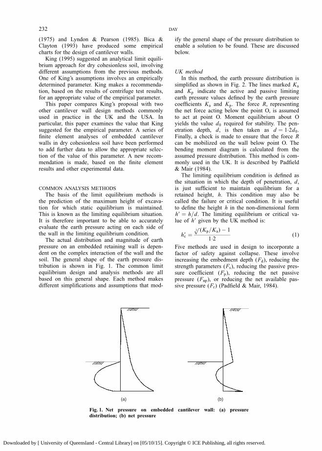
The actual distribution and magnitude of earthpressure on an embedded retaining wall is depen-dent on the complex interaction of the wall and thesoil. The general shape of the earth pressure dis-tribution is shown in Fig. 1. The common limitequilibrium design and analysis methods are allbased on this general shape. Each method makesdifferent simpli®cations and assumptions that mod-

ify the general shape of the pressure distribution toenable a solution to be found. These are discussedbelow.

UK methodIn this method, the earth pressure distribution is

simpli®ed as shown in Fig. 2. The lines marked Ka

and Kp indicate the active and passive limitingearth pressure values de®ned by the earth pressurecoef®cients Ka and Kp. The force R, representingthe net force acting below the point O, is assumedto act at point O. Moment equilibrium about Oyields the value d0 required for stability. The pen-etration depth, d, is then taken as d � 1:2d0.Finally, a check is made to ensure that the force Rcan be mobilized on the wall below point O. Thebending moment diagram is calculated from theassumed pressure distribution. This method is com-monly used in the UK. It is described by Pad®eld& Mair (1984).

The limiting equilibrium condition is de®ned asthe situation in which the depth of penetration, d,is just suf®cient to maintain equilibrium for aretained height, h. This condition may also becalled the failure or critical condition. It is usefulto de®ne the height h in the non-dimensional formh9 � h=d. The limiting equilibrium or critical va-lue of h9 given by the UK method is:

h9c ��

3p

(Kp=Ka)ÿ 1

1:2(1)

Five methods are used in design to incorporate afactor of safety against collapse. These involveincreasing the embedment depth (Fd), reducing thestrength parameters (Fs), reducing the passive pres-sure coef®cient (Fp), reducing the net passivepressure (Fnp), or reducing the net available pas-sive pressure (Fr) (Pad®eld & Mair, 1984).

(a) (b)

Fig. 1. Net pressure on embedded cantilever wall: (a) pressuredistribution; (b) net pressure

232 DAY


USA methodIn this method, the earth pressure distribution is

simpli®ed by the rectilinear distribution shown inFig. 3. The rectilinear distribution is characterizedby the parameters pa, p1, p2 and y. This is amodern version of a method initially proposed byKrey in 1932. It is described by Bowles (1988)and King (1995). This method is commonly usedin the USA.

For a given retained height, h, it is required todetermine the minimum depth of penetration andthe corresponding pressure distribution that justmaintains stability ± the limiting equilibrium solu-tion. In this situation, it is reasonable to assumethat the pressure behind the wall at the dredgelevel, pa, is equal to the active pressure limit.Hence, there are four unknown values, d, p1, p2

and y, which need to be determined.The consideration of horizontal force and mo-

ment equilibrium provides two equations. In orderto obtain a solution, two more assumptions arenecessary. In the USA method these assumptionsare as follows:

(a) The limiting passive pressure is fully mobi-lized on the wall immediately below dredgelevel. This assumption gives the gradient of therectilinear pressure distribution between pa andp1. It is equal to the passive pressure gradientminus the active pressure gradient, ã(Kpÿ Ka),where ã is the bulk unit weight of the soil.

(b) The value of p2 is equal to the passivepressure limit on the retained side minus theactive pressure on the dredged side (equation(2)). This is the maximum possible valuewhich p2 can have:

p2 � ã(h� d)Kp ÿ ãdKa (2)

The equations of equilibrium and the constraintsimposed by the two assumptions yield equation (3)(King, 1995). For a given value of h, this equationcan be solved for Y and hence the limiting equili-brium depth of penetration d, and h9c:

Y 4 � q

m

� �Y 3 ÿ 8P

m

� �Y 2 ÿ 6P

m2(2mb� q)Y

ÿ P

m2(6bq� 4P) � 0 (3)

where

q � Kpã(h� x)ÿ Kaãx; m � (Kp ÿ Ka)ã

b � (h� 2x)

3; x � Kaãh

m(4)

P � 12Kaãh(h� x)

Two methods are used in design to incorporate afactor of safety against collapse. Either the embed-ment depth is increased by 30% or a factor of safetyis used to reduce the passive pressure coef®cient.

GENERAL RECTILINEAR NET PRESSURE METHOD

This method proposed by King (1995) is similarto the USA method. The earth pressure is simpli-®ed by a similar rectilinear net pressure distribu-

(a) (b)

h

dR

Ka

O

Ka

Kp

R

Kpd 0

Ka

0.2d0

Fig. 2. Simpli®ed pressure distribution ± UK method: (a) pressure distribu-tion; (b) net pressure

h

d

Ka

pa

p2

Y

x

p1

ε

y

Fig. 3. Rectilinear pressure distribution

NET PRESSURE ANALYSIS OF CANTILEVER SHEET PILE WALLS 233


tion (Fig. 3). Force and moment equilibrium andthe ®rst of the assumptions made in the USAmethod provide three equations or conditions. Thegeneral rectilinear net pressure method differs fromthe USA method only in the second assumptionrequired to obtain a solution. The second assump-tion involves the location of the point, near thebottom of the wall, of zero net pressure. King(1995) suggested that the assumption å9 �å=d � 0:35 (Fig. 3) provided good predictions offailure height and bending moment distribution.This recommendation was based on the results ofcentrifuge tests. The advantage of this method isthat the value of p2 is not prescribed as beingequal to its maximum possible value.

Application of the general rectilinear methodForce and moment equilibrium yield the follow-

ing two equations (King, 1995):

x9 � y9[(1ÿ 2å9)ÿ y9(1ÿ å9)]

h9(1ÿ å9ÿ y9)ÿ y92 � (1ÿ 2å9)(5)

and

[(1ÿ å9)h9� (1ÿ 2å9)]y92 � [(1ÿ å9)h92

ÿ (1ÿ 3å9)]y9ÿ [(1ÿ 2å9)h92 � (1ÿ 3å9)h9] � 0

(6)

where x9 � x=d, h9 � h=d, y9 � y=d, and å9 �å=d.

Thus for a given value of h9 and an assumedvalue of å9, the values of y9 and x9 can bedetermined from equations (5) and (6). The recti-

linear pressure distribution is then fully de®ned interms of the non-dimensional parameters x9, y9 andå9. However, the depth of embedment, d, remainsunknown. It is interesting to note that equations (5)and (6) are dependent only on the geometricalparameters. They are independent of the soil den-sity and the active and passive pressure coef®cientsKa and Kp.

The ®rst assumption of the rectilinear pressuredistribution de®nes the distance x (Fig. 3) at limit-ing equilibrium:

x

pa

� 1

ã(Kp ÿ Ka)(7)

where, pa � ãhKa

The limiting equilibrium or failure criteria cantherefore be expressed in the form (King, 1995)

x

h

� �c

� x9

h9

� �c

� 1

Kp=Ka ÿ 1(8)

Using equations (5) and (6), the relationship be-tween x9=h9 and h9 can be calculated for differentvalues of å9 (Fig. 4). For a particular situation (Ka

and Kp given by soil strength and wall frictionangles), the critical value of h9 can therefore bedetermined using Fig. 4 and equation (8) with theassumed value of å9.

EXAMINATION OF THE METHODS

General rectilinear net pressure methodFrom Fig. 4 it can be seen that for the larger

values of å9 there is a maximum value of x=h. In

101

100

1022

1023

1021

0.1 1.0 10.0

h ′ 5 h/d

x′/h

′ 5 x

/h

Value of ε ′0.33

0.30

0.25

0.34

0.35 0.36

0.380.40

258

208

308

(x/h)c for :

Fig. 4. Relationship between x=h and h9

234 DAY


fact, if å9 is greater than 1=3, there exists a maxi-mum value for x=h (not shown on ®gure). If thecritical value of x=h given by equation (8) isgreater than this maximum, then a solution whichsatis®es the equations of equilibrium and the as-sumed value of å9 does not exist. Fig. 4 alsoillustrates that if the critical value of x=h is lessthan the maximum value, there are two validsolutions for h9 which satisfy the assumptions, thelarger value being of practical interest.

The critical values of x=h calculated from equa-tion (8) for the case of a frictionless wall areshown in Fig. 4 for ö9 � 208, 258 and 308. Forthese cases, Kp=Ka � 4:2, 6´1 and 9´0 respectively.The recommendation of King, that å9 is assumedconstant and equal to 0´35, does not yield a solu-tion if Kp=Ka is less than 7´90 (e.g. frictionlesswalls in low-strength soils). In practice, however, asolution is possible.

Clearly, this is a de®ciency. It would appear that,for situations with lower values of Kp=Ka, thevalue of å9 at limiting equilibrium is less than0´35.

Failure depth of excavationEquations (1) and (8) indicate that the critical

retained height h9c is dependent only on the ratioKp=Ka. The variation of h9c calculated using eachmethod is plotted in Fig. 5 for a range of values ofKp=Ka. The range of possible values of Kp=Ka isvery large. For a frictionless wall in a ö9 � 208material, Kp=Ka � 4:2, and for a rough wall in aö9 � 508 material, Kp=Ka � 477. The critical va-lues predicted by the rectilinear net pressure meth-od are plotted for a range of assumed values of å9.

Figure 5 highlights the following interestingpoints:

(a) The UK and USA methods predict values thatlie on lines nearly parallel to lines of constant å9.

(b) The UK method is very close over the wholerange of Kp=Ka to the rectilinear net pressuremethod if a value of å9 � 0:27 is assumed.

(c) The assumptions of the USA method yield avalue of å9 that varies between about 0´1 athigh values of Kp=Ka and 0´15 at low values(see also Fig. 18).

(d) King's recommendation of å9 � 0:35 is moreconservative than both the UK and the USAmethods.

FINITE ELEMENT ANALYSES

A series of two-dimensional plane strain ®niteelement analyses have been performed to deter-mine the pressure distribution on an embeddedcantilever wall at limiting equilibrium for compari-son with that assumed in the limit equilibriummethods described above. In the ®nite elementanalyses, the limiting equilibrium height of excava-tion was determined by `excavating' elements fromthe mesh in front of a 10 m deep wall untilnumerical convergence was not achieved. Detailsof the mesh and boundary conditions are shown inFig. 6. The displacement of the top of the wall isplotted against the excavation depth in Fig. 7. Thisplot is necessary to ensure that the failure toconverge was indeed due to a physical instabilityof the wall, rather than a numerical problem.Before excavation began, the initial horizontalstress in the soil was equal to half the vertical

Value of ε ′

1 10 100 1000

6

5

4

3

2

1

0

0.270.20

0.10

0.30

0.350.40

Rectilinear net pressure

UK method

USA (Bowles, 1988)

Kp/Ka

h′ c

5 h

c/d

Fig. 5. Critical height of excavation



stress (K0 � 0:5). Analyses by Fourie & Potts(1989) and Day & Potts (1993) have shown thatthe initial value of K0 does not affect the failureheight of excavation. The analyses assume fullydrained conditions with pore pressure equal to zeroand are therefore applicable to the long-term con-

dition. The Imperial College Finite Element Pro-gram was used for the analyses.

An elastic±perfectly plastic cohesionless Mohr±Coulomb model was used to describe the soilbehaviour. A range of analyses was performed withthe friction angle, ö9, of the soil equal to 208, 258,

508

10

5

000

Scale 1Scale 2

100500

2001000

458408 358

308

258

208

Exc

avat

ion

heig

ht: m

Low stifness (scale 2)

Middle stiffness (scale 1)

High stiffness (scale 1)

Deflection: mm

Fig. 7. De¯ection of top of wall

20 mWall

10 m

50 m

120 m

Fig. 6. Finite element mesh ± excavated elements cross-hatched

236 DAY


308, 358, 408, 458 and 508. In each case, the angleof dilation was taken as half the friction angle.The bulk unit weight of the soil, ã, equals20 kN=m3. The Young's modulus equals 5000 �5000z kPa, where z is the depth measured from theoriginal ground surface. The Poisson's ratio equals0´2.

The wall was assumed to be elastic with proper-ties equivalent to a reasonably stiff sheet pile:E � 2:1 3 108 kPa, I � 46:8 3 10ÿ4 m4=m width,and A � 5:26 3 10ÿ2 m2=m. The wall was as-sumed to be rough in all analyses. For the cases ofsoil strength, ö9 � 208, 358 and 508, additionalanalyses were done using walls 100 times less stiffand 100 times more stiff in bending (I � 46:8 310ÿ6 m4=m, A � 1:13 3 10ÿ2 m2=m and I � 46:83 10ÿ2 m4=m, A � 24:4 3 10ÿ2 m2=m).

ANALYSIS OF RESULTS

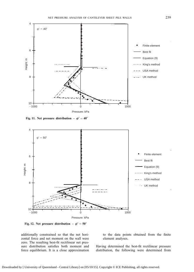
The net horizontal earth pressure on the wallobtained from the ®nite element analyses at limit-ing equilibrium at the integration points is shownin Figs 8±12 for the analyses using ö9 � 208, 258,358, 408 and 508. The upper 4 m of the wall, onwhich the pressure distribution is linear, has beenomitted for clarity. The results of the other ana-lyses are similar. For the cases of ö9 � 208, 358and 508, the results of the analyses with differentwall stiffness are similar to the results shown. Thelimiting equilibrium height of excavation is also

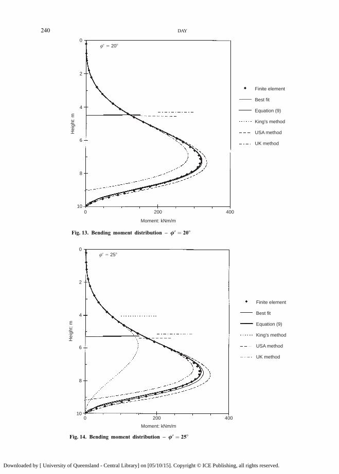
marked on these ®gures by a horizontal line. Thiswas taken as the last height at which numericalconvergence was achieved and is estimated to havean accuracy of 0´1 m. The bending moment distri-butions in the wall for these analyses are shown inFigs 13±17. The results of the other analyses aresimilar.

Net pressure distributionThe integration point stress distributions indicate

that the net pressure distribution is characterizedby a linear part above the excavation level and alinear part immediately below the excavation level,extending almost to the point of the maximumvalue. Below the maximum, to the bottom of thewall the net pressure is non-linear. The wall stiff-ness has very little effect on the limiting equili-brium excavation height and the net pressure onthe wall at failure.

The aim of the ®nite element analyses was todetermine the validity of the assumptions used inthe rectilinear net pressure method. Hence, therectilinear pressure distribution shown in Fig. 3was ®tted to the net pressure data points (integra-tion points) obtained from the ®nite element ana-lyses. The best-®t line is plotted in Figs 8±12. Therectilinear best-®t approximation was found in thefollowing way:

(a) Using a least squares ®t to the bending

Finite element

Best fit

Equation (9)

King's method

USA method

UK method

Pressure: kPa

21000 0 1000

φ′ 5 208

4

6

8

10

Hei

ght:

m

Fig. 8. Net pressure distribution ± ö9 � 208



moment data points above the excavation level,the value of pa was determined. The bendingmoment was used instead of the stressesbecause the bending moment is very sensitiveto small changes in the pressure.

(b) Using this value of pa, the values of p1, p2

and y were determined by a least squares ®t ofthe rectilinear pressure distribution to the ®niteelement net pressure data points over the fullwall length. The values of p1, p2 and y were

Finite element

Best fit

Equation (9)

King's method

USA method

UK method

Pressure: kPa

21000 0 1000

φ′ 5 358

Hei

ght:

m

4

6

8

10


Finite element

Best fit

Equation (9)

King's method

USA method

UK method

Pressure: kPa

21000 0 1000

φ′ 5 258

4

6

8

10

Hei

ght:

m


238 DAY


additionally constrained so that the net hori-zontal force and net moment on the wall werezero. The resulting best-®t rectilinear net pres-sure distribution satis®es both moment andforce equilibrium. It is a close approximation

to the data points obtained from the ®niteelement analyses.

Having determined the best-®t rectilinear pressuredistribution, the following were determined from

Finite element

Best fit

Equation (9)

King's method

USA method

UK method

Pressure: kPa

21000 0 1000

φ′ 5 508

Hei

ght:

m

4

6

8

10


Finite element

Best fit

Equation (9)

King's method

USA method

UK method

Pressure: kPa

21000 0 1000

φ′ 5 408H

eigh

t: m

4

6

8

10




Finite element

Best fit

Equation (9)

King's method

USA method

UK method

Moment: kNm/m

Hei

ght:

m

0

2

4

6

8

100 200 400

φ′ 5 258

Fig. 14. Bending moment distribution ± ö9 � 258

Finite element

Best fit

Equation (9)

King's method

USA method

UK method

Moment: kNm/m

Hei

ght:

m

0

2

4

6

8

100 200 400

φ′ 5 208


240 DAY


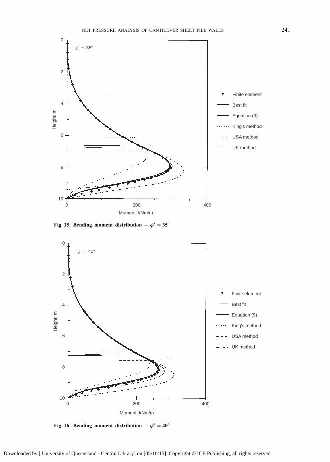
Finite element

Best fit

Equation (9)

King's method

USA method

UK method

Moment: kNm/m

0 200 400

φ′ 5 408

Hei

ght:

m

0

2

4

6

8

10


Finite element

Best fit

Equation (9)

King's method

USA method

UK method

Moment: kNm/m

Hei

ght:

m

0

2

4

6

8

100 200 400

φ′ 5 358




the values of pa, p1, p2, y and the wall geometry,h and d:

(a) The distance from the bottom of the wall ofzero net pressure, å9.

(b) The active pressure coef®cient, Ka. In allcases, Ka was within 2% of the theoreticalvalue given by Caquot & Kerisel (1948) for arough wall.

(c) The passive pressure coef®cient immediatelybelow the excavation level, Kp, that is inferredfrom the rectilinear pressure distribution be-tween pa and p1.

For comparison with the value of Kp inferred fromthe best-®t rectilinear pressure distribution (above),Kp was also determined from the ®nite elementintegration point stresses. This was calculated usinga least squares ®t to the linear part of the passivepressure distribution immediately below the exca-vation.

The values of å9 determined in this manner areplotted against Kp=Ka in Fig. 18 for Kp deter-mined in three different ways. The values of Kp

used are the theoretical values given by Caquot &Kerisel (1948) for a rough wall, and those calcu-lated by the two methods described above. It can

be seen that there is very little difference betweenthe different methods. Therefore, the theoreticalpassive pressure is fully mobilized below the ex-cavation level and the ®rst assumption used in therectilinear net pressure method is quite reasonable.Also plotted on this diagram are the values of å9that result from the assumptions used to de®ne thenet pressure distribution in the USA method.

Clearly, å9 is not constant and varies with re-spect to the limiting earth pressures (Kp=Ka). Agood approximation to the actual value is given byequation (9), which is plotted on Fig. 18:

å9 � 0:047 lnKp

Ka

� �� 0:1 (9)

The net pressure distribution and the predictedlimiting equilibrium height of excavation given bythe UK method, USA method, King's recommenda-tion (å9 � 0:35) and equation (9), in conjunctionwith theoretical pressure coef®cients Ka and Kp

given by Caquot & Kerisel (1948), are also plottedon Figs 8±12. This is akin to a design procedure.It is noted that King's assumption does not yield asolution in the case of ö9 � 208, because Kp=Ka isless than 7´9. There is good agreement between theresults based on equation (9) and the ®nite element

Finite element

Best fit

Equation (9)

King's method

USA method

UK method

Moment: kNm/m

Hei

ght:

m

0

2

4

6

8

100 200 400

φ′ 5 508


242 DAY


results. Neither the USA method nor the assump-tion that å9 � 0:35 produces good estimates of thelimiting equilibrium height and net earth pressureover the full range of soil properties and wallfriction. The USA method is reasonably good forlow values of Kp=Ka, and King's assumption isreasonable at high values. Consequently, the USAmethod and the å9 � 0:35 assumption produce er-roneous bending moment distributions comparedwith the ®nite element results.

Bending moment at limiting equilibriumIn Figs 13±17 the bending moments calculated

from the best-®t rectilinear net pressure are plotted.The best-®t rectilinear net pressure diagram pro-duces a bending moment that is surprisingly closeto the ®nite element bending moment. The bendingmoment obtained from the USA method, King'sassumption (å9 � 0:35), equation (9) and the UKmethod in conjunction with theoretical values ofKa and Kp are also shown.

Comparison of methodsThe limiting equilibrium retained height ob-

tained from the ®nite element analysis is the laststable height for which a numerical solution wasobtained. It is estimated that the actual criticalheight is up to 0´1 m greater. The consequentialrange in h9c is plotted in Fig. 19 against the ratioKp=Ka. The values of Ka and Kp used here weredetermined from the integration point stresses inthe soil immediately adjacent to the wall (as de-scribed above). Also plotted are the results of

centrifuge tests reported by King (1995). The cen-trifuge experiments were performed by excavationof 0´5 m of soil at each stage (the wall was 11 mlong). The actual limiting equilibrium height maytherefore be up to 0´5 m greater than the lastobserved stable height, which is reported by King.This range is plotted in Fig. 19. There is excellentagreement between the ®nite element results andthe centrifuge data. The limiting equilibrium heightpredicted by the rectilinear pressure distributionbased on the assumptions that passive pressure isfully mobilized immediately below excavation andå9 is given by equation (9) is also plotted in Fig.19. This method provides an excellent predictionof the ®nite element results and the centrifuge dataover the full range of Kp=Ka.

The predictions of critical retained height andbending moment distribution by the USA and UKmethods are reasonable at low values of Kp=Ka

but not at high values. The assumption ofå9 � 0:35 is in better agreement with the data and®nite element results at the upper values of Kp=Ka

but appears very conservative at lower values.

CONCLUSION

A rectilinear net pressure distribution comprisingthree lines provides a good approximation to the actualnet pressure distribution at limiting equilibrium. Thisdistribution has the following characteristics:

(a) Active pressure is fully mobilized above theexcavation level.

(b) Passive pressure is fully mobilized immedi-ately below the excavation level.

0.5

0.4

0.3

0.2

0.1

0.0

ε′

1 10 100 1000

Kp/Ka

ε ′ 5 0.047 ln(Kp/Ka) 1 0.10

USA (Bowles, 1988)

FE stresses

Best fit

Theoretical

Fig. 18. Position of zero net pressure



(c) The point of zero net pressure is dependent onthe active and passive pressure coef®cients andis de®ned by equation (9).

The limiting equilibrium retained height and thebending moment distribution predicted by this rec-tilinear net pressure are in excellent agreementwith centrifuge data and ®nite element analysesover the full range of soil strength and wall frictioncoef®cients.

The proposal by King (1995) that å9 � 0:35 isgenerally conservative. The predicted limiting equi-librium retained height and maximum bending mo-ment are generally less than is indicated by the®nite element data. This is particularly so wherethe value of Kp=Ka is low. In some cases, such aslow-strength soil and/or frictionless wall, the as-sumption that å9 � 0:35 will not yield a solutionwhere one is clearly physically possible.

Equation (9), the rectilinear net pressure distri-bution and pressure coef®cients given by Caquot &Kerisel (1948), may be used as a design method topredict the limiting equilibrium retained height andbending moment distribution. Such predictions willbe more accurate than existing design methodscommonly used in the UK and USA.

These recommendations allow accurate calcula-tion of the limiting equilibrium or limit state situa-tion. For safety and serviceability, the depth ofexcavation will, of course, be less than the limitingvalue. Further investigation is required to deter-mine whether a rectilinear pressure distribution

may be as good an approximation to the net pres-sure in the realistic situations when the retainedheight is less than the limit state value. The in situstress (K0) and wall stiffness are likely to be moresigni®cant in this situation.

REFERENCESBica, A. V. D. & Clayton, C. R. I. (1989). Limit equi-

librium design methods for free embedded cantileverwalls in granular materials. Proc. Instn Civ. EngrsPart 1 86, 879±989.

Bica, A. V. D. & Clayton, C. R. I. (1993). The prelimin-ary design of free embedded cantilever walls ingranular soil. In Retaining structures (ed. C. R. I.Clayton), pp. 731±740. London: Thomas Telford.

Bowles, J. E. (1988). Foundation analysis and design, 4thedn. New York: McGraw-Hill.

Bransby, J. E. & Milligan, G. W. E. (1975). Soil deforma-tions near cantilever retaining walls. GeÂotechnique 24,No. 2, 175±195.

Caquot, A. & Kerisel, J. (1948). Tables for the calculationof passive pressure, active pressure and bearing pres-sure of foundations. Paris: Gauthier-Villars.

Day, R. A. & Potts, D. M. (1993). Modelling sheetpile retaining walls. Computers Geotechnics 15,125±143.

Fourie, A. B. & Potts, D. M. (1989). Comparison of ®niteelement and limiting equilibrium analyses for anembedded cantilever wall. GeÂotechnique 39, No. 2,175±188.

King, G. J. W. (1995). Analysis of cantilever sheet-pilewalls in cohesionless soil. J. Geotech. Engng Div.,ASCE 121, No. 9, 629±635.

Kp/Ka

ε ′ 5 equation (9)

1 10 100 1000

6

5

4

3

2

1

0

Centrifuge (King, 1995)

Finite elementUSA

UKε ′ 5 0.35

h′ c

5 h

c/d

Fig. 19. Comparison of ®nite element results, centrifuge data and design methods

244 DAY


Lyndon, A. & Pearson, R. A. (1985). Pressure distributionon a rigid retaining wall in cohesionless material.Proceedings of international symposium on applica-tion of centrifuge modelling to geomechanics de-sign (ed. W. H. Craig), pp. 271±280. Rotterdam:Balkema.

Pad®eld, C. J. & Mair, R. J. (1984). Design of retainingwalls embedded in stiff clays, Report 104. London:Construction Industry Research and Information Asso-ciation.

Rowe, P. W. (1951). Cantilever sheet piling in cohesion-less soil. Engineering September 7, 316±319.



Net pressure analysis of cantilever sheet pile walls · Net pressure analysis of cantilever sheet...

Documents

Transcript of Net pressure analysis of cantilever sheet pile walls · Net pressure analysis of cantilever sheet...