10TH INTERNATIONAL SYMPOSIUM ON PARTICLE IMAGE VELOCIMETRY - PIV13Delft, The Netherlands, July 1-3, 2013

Nested multi-resolution PIV measurements of wall bounded turbulence athigh Reynolds numbers

C. M. de Silva1, C. Atkinson2, N. A. Buchmann2, E.P. Gnanamanickam1, N. Hutchins1, J. Soria2,3 and I.Marusic1

1Department of Mechanical Engineering, The University of Melbourne, Victoria 3010, Australia.2Laboratory for Turbulence Research in Aerospace & Combustion, Department of Mechanical and Aerospace

Engineering, Monash University, Victoria 3800, Australia.3Department of Aeronautical Engineering, King Abdulaziz University, Jeddah, Kingdom of Saudi Arabia.

ABSTRACT

Here we describe the use of a nested high magnification camera configuration within a large field of view (FOV) PIV experiment.The objective of these measurements is to obtain instantaneous velocity flow fields to resolve the wide range of scales present inturbulent boundary layers at high Reynolds numbers of up to Reτ ≈ 20000. Flow statistics are compared against previous measurementsmade using hot-wire anemometry to validate and assess the quality of the PIV velocity fields. Preliminary analysis shows that theinstantaneous wall shear stress can be computed from the experimental data, enabling us to directly compute quantities such as thefriction velocity.

1. Introduction

Particle image velocimetry (PIV) has become increasingly popular over the last decade for accurately measuring multi-component,multi-dimensional velocity fields associated with turbulent flows. More recently, due to the advancement and increase in resolution ofPIV cameras, studies have shown that PIV techniques can be effectively applied with spatial resolutions of the order of a few microns[Kahler et al., 2012]. Here we describe the application of such a technique to simultaneously obtain a large FOV while also resolvingthe small scales in the near wall region of a high Reynolds number turbulent boundary layer by using varying magnifications. Theapplication to high Reynolds number flows further emphasises the importance of having varying resolutions; a large FOV is necessaryto capture the larger structures, which scale with the boundary layer thickness (≈ 0.35m). Conversely, the smaller scales associated withthe near wall cycle scale with inner viscous units (ν/Uτ ≈ 45µm at Reτ ≈ 8000) and require high spatial resolution.

The novelty of the data-set presented is the ability to obtain well resolved instantaneous velocity fields at close proximity to the wall(approaching the viscous sublayer), within a large FOV. This enables us to quantitatively analyse large scale structures in the logarithmicand outer regions of the boundary layer and their associated modulating effect on near wall structures [Marusic et al., 2010].

Here, we use the coordinate system x, y and z to refer to the streamwise, spanwise and wall-normal directions respectively. Theinstantaneous stream-wise velocity and wall-normal velocity are represented by U and W respectively, with corresponding fluctuatingvelocity components given by u, v and w. Capitalisation and overbars indicate averaged quantities. The superscript + refers tonormalisation with the inner scales. For example, we use l+ = lUτ/ν for length and U+ = U/Uτ for velocity, where Uτ is the frictionvelocity and ν is the kinematic viscosity of the fluid.

2. Experimental setup

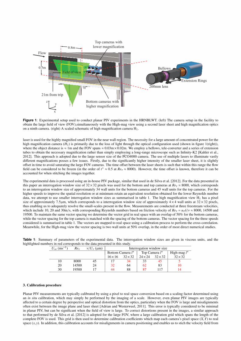
The experiments are performed in the High Reynolds Number Boundary Layer Wind Tunnel (HRNBLWT) at the University ofMelbourne. Figure 1 shows an overall view of the experimental setup which is located 21m downstream of the trip. The longdevelopment length enables us to obtain high Reynolds numbers at relatively slow freestream velocities, which results in a largerviscous length scale, and hence less acute spatial resolution issues. The imaging system used to obtain the large field of view (FOV)of approximately 0.8m×0.5m (detailed further in de Silva et al. [2012]) consists of eight PCO4000 cameras (4008×2672 pixels, 2Hz)arranged as shown in figure 1. It is desirable to capture the large scale structures that have length scales the order of the boundary layerthickness (δ) with a large FOV. Meanwhile the use of multiple cameras enables us to maintain adequate spatial resolution to resolvemost of the smaller length scales, which are the order of the Kolmogorov length scales (η). At high Reynolds numbers this task isfurther complicated since the ratio δ/η is large (≈ 103 for the flow studied here). To overcome this, a higher magnification is used in thenear-wall and log region where we expect a larger contribution of the turbulent energy to be from small scales. Meanwhile for the outerregion, a lower magnification is used that is capable of resolving the dominant larger scale structures prevalent here. The novelty of themeasurements presented here is the use of a ninth PCO4000 camera simultaneously to obtain a highly magnified (High-mag) view inthe near wall region, which is nested within the larger FOV (shown in figure 2).

The particles are illuminated by two laser sheets overlapped in the spanwise direction, and created using two Spectra Physics ‘Quanta-Ray’PIV 400 Nd:YAG double-pulse lasers that deliver 400mJ/pulse. One laser is dedicated to illuminating the large FOV, and the second

Flow

0.8m

0.5m

Field of view

Bottom cameras with

higher magnification

Top cameras with

lower magnification

z

x

y

21m from trip

Bellows

Extension Rings

200mm lens

Figure 1: Experimental setup used to conduct planar PIV experiments in the HRNBLWT. (left) The camera setup in the facility toobtain the large field of view (FOV),simultaneously with the High-mag view using a second laser sheet and high magnification opticson a ninth camera. (right) A scaled schematic of high magnification camera H1.

laser is used for the highly magnified small FOV in the near wall region. The necessity for a large amount of concentrated power for thehigh magnification camera (H1) is primarily due to the loss of light through the optical configuration used (shown in figure 1(right)),where the object distance is ≈ 1m and the FOV spans ≈ 0.03m×0.02m. We employ a bellows, tele-converter and a series of extensiontubes to obtain the necessary magnification rather than simply employing a long-range microscope such as Infinity-K2 [Kahler et al.,2012]. This approach is adopted due to the large sensor size of the PCO4000 camera. The use of multiple lasers to illuminate vastlydifferent magnifications posses a few issues. Firstly, due to the significantly higher intensity of the smaller laser sheet, it is slightlyoffset in time to avoid saturating the large FOV cameras. The time offset between the laser sheets is such that within this range the flowfield can be considered to be frozen (in the order of t+ ≈ 0.5 at Reτ ≈ 8000). However, the time offset is known, therefore it can beaccounted for when stitching the images together.

The experimental data is processed using an in-house PIV package, similar that used in de Silva et al. [2012]. For the data presented inthis paper an interrogation window size of 32× 32 pixels was used for the bottom and top cameras at Reτ ≈ 8000, which correspondsto an interrogation window size of approximately 34 wall units for the bottom cameras and 45 wall units for the top cameras. For thehigher speeds to improve the spatial resolution or at minimum retain an equivalent resolution obtained for the lower Reynolds numberdata, we attempt to use smaller interrogation window sizes as summarised in table 1. The high magnification view H1 has a pixelsize of approximately 7.5µm, which corresponds to a interrogation window size of approximately 4× 4 wall units at 32× 32 pixels,thus enabling us to adequately resolve the small-scales present in the flow. Measurements are conducted at three freestream velocities,which include 10, 20 and 30m/s, with corresponding Reynolds numbers based on friction velocity of Reτ = uτδ/ν ≈ 8000, 14500 and19500. To maintain the same vector spacing we determine the vector grid in real space with an overlap of 50% for the bottom cameras,while the vector spacing for the top camera is matched with the spacing of the bottom cameras. The vector spacing for the three speedsconsidered is summarised in table 1. The vectors are mapped to real space using a calibration process to perform the cross-correlation.Meanwhile, for the High-mag view the vector spacing is two wall units at 50% overlap, in the order of most direct numerical studies.

Table 1: Summary of parameters of the experimental data. The interrogation window sizes are given in viscous units, and thehighlighted numbers in red corresponds to the data presented in this study.

U∞ (ms−1) Reτ ν/Uτ (µm) Interrogation window sizeBottom Camera l+ Top Camera l+ High-mag l+

16×16 32×32 24×24 32×32 32×3210 8000 45 17 34 33 45 520 14500 24 32 64 62 83 1030 19500 17 44 88 87 117 14

3. Calibration procedure

Planar PIV measurements are typically calibrated by using a pixel to real space conversion based on a scaling factor determined usingan in situ calibration, which may simply be performed by the imaging of a scale. However, even planar PIV images are typicallyaffected to a certain degree by perspective and optical distortion from the optics, particulary when the FOV is large and misalignmentsoften exist between the image plane and laser sheet [Adrian and Westerweel, 2011]. This error is typically considered to be minimalin planar PIV, but can be significant when the field of view is large. To correct distortions present in the images, a similar approachto that performed by de Silva et al. [2012] is adopted for the large FOV, where a large calibration grid which spans the length of thecomplete FOV is used. This grid is then used to determine calibration coefficients which map each camera’s pixel space (X,Y) to realspace (x,y). In addition, this calibration accounts for misalignments in camera positioning and enables us to stich the velocity field from

Stream-wise x/δ

Wall-normal

z/δ

B1 B2 B3 B4

T1 T2 T3 T4

0 0.5 1 1.5 2

0

0.2

0.4

0.6

0.8

1

1.2

1.4

5

6

7

8

9

10

11

12

−0.1 0 0.1 0.2 0.3 0.4 0.5 0.6 0.7 0.8

0

0.1

0.2

0.3

0.4

0.5

x(m)

z(m

)

x(m)

z(m

)

0.19 0.21

0.005

0.01

0.015

0.02

x(m)

z+

0.19 0.21

100

200

300

400

0

1

2

3

4

5

6

7

U

U

(a)

(b) Large FOV (c) High−mag view − H1

H1

∆ x ≈ 3cm

∆ z ≈ 2cm

Figure 2: (a) shows the FOV across the eight cameras (L1−4 and T1−4), H1 indicates the location of the high magnification view nestedwithin the larger FOV in the near wall region. The location x = 0 is located 21m downstream of the trip. (b) Shows the instantaneousstreamwise velocity vectors seen by the large FOV in the region captured by H1, meanwhile (c) shows the same region as seen with thehigh magnification camera.

multiple cameras by precisely locating each camera’s position relative to the others. The calibration grid used for the large FOV hasa grid spacing of 5mm. However for the High-mag view, which only spans a few centimeters in width a smaller machined calibrationgrid with 1mm spacing was necessary.

Precisely locating the wall position is a key issue for most measurements in wall-bounded flows, and is particularly so when consideringa streamwise wall-normal plane in PIV experiments due to wall reflections caused by the laser sheet [Adrian and Westerweel, 2011].Here we use the calibration grid to assist us in locating the wall location relative to the four lower cameras, using the reflection ofthe calibration grid on the glass wall and the estimated pixel position of the wall in each camera (detailed further in de Silva et al.[2012]). It should be noted that similar to the calibration process detailed previously it is essential to first map the image to real spaceusing the calibration coefficients prior to computing the estimated wall position. This method was previously shown to work well fora similar large FOV experiment [de Silva et al., 2012]. Here we extend this technique and conclude that a similar technique providesacceptable accuracy for the highly magnified view, based on the mean streamwise velocity (shown in figure 3(a)), which is obtainedwithout applying any shift to the wall position of the velocity fields. However, we note that there can be very small errors in relation tothe positioning of the calibration target and imperfections on the glass wall, but results indicate this error to be well below 100µm (asevidenced by the collapse of the mean velocity profile to z+ < 3).

4. Results

4.1 Mean and turbulence intensity flow statisticsThe main novelty in the measurements detailed is the range of magnifications simultaneously employed to resolve the range of scalespresent in a high Reynolds number flow. Figure 2a shows the layout of all the nine cameras, with contours of instantaneous streamwise

velocity overlayed. Figure 2(a) gives a good visual indication of the range of length scales associated with such high Reynolds numberflows. Figure 2(b) shows a cut out of the large FOV which is simultaneously captured by the high magnification camera (shown infigure 2c). Comparisons between figure 2(b) and 2(c) clearly shows the loss of small scale information in the large FOV, in addition tothe lack of reliable data below a wall position of 75 wall units in z which is also evident in the flow statistics shown in the later part ofthis paper. We see that the High-mag view is resolved much better and also has reliable velocity vectors significantly closer to wall.

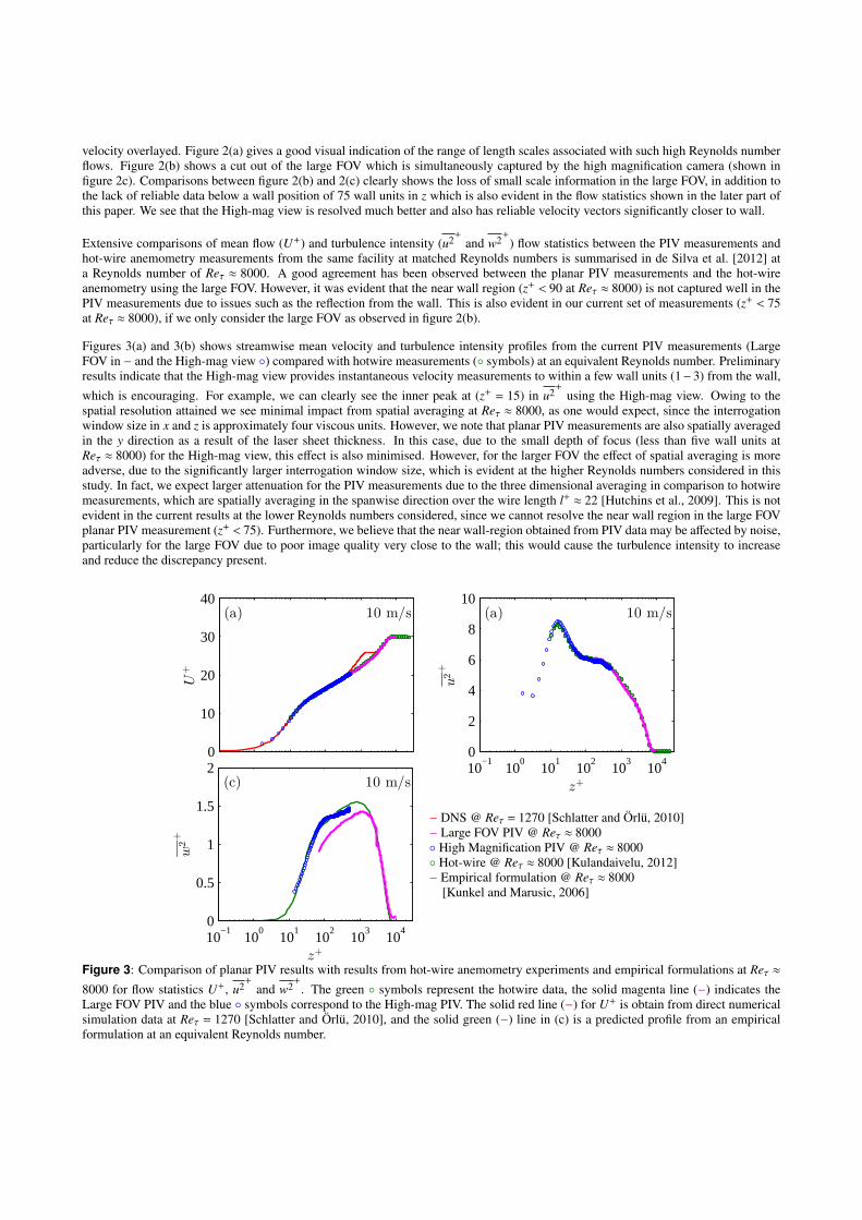
Extensive comparisons of mean flow (U+) and turbulence intensity (u2+

and w2+

) flow statistics between the PIV measurements andhot-wire anemometry measurements from the same facility at matched Reynolds numbers is summarised in de Silva et al. [2012] ata Reynolds number of Reτ ≈ 8000. A good agreement has been observed between the planar PIV measurements and the hot-wireanemometry using the large FOV. However, it was evident that the near wall region (z+ < 90 at Reτ ≈ 8000) is not captured well in thePIV measurements due to issues such as the reflection from the wall. This is also evident in our current set of measurements (z+ < 75at Reτ ≈ 8000), if we only consider the large FOV as observed in figure 2(b).

Figures 3(a) and 3(b) shows streamwise mean velocity and turbulence intensity profiles from the current PIV measurements (LargeFOV in − and the High-mag view ◦) compared with hotwire measurements (◦ symbols) at an equivalent Reynolds number. Preliminaryresults indicate that the High-mag view provides instantaneous velocity measurements to within a few wall units (1−3) from the wall,

which is encouraging. For example, we can clearly see the inner peak at (z+ = 15) in u2+

using the High-mag view. Owing to thespatial resolution attained we see minimal impact from spatial averaging at Reτ ≈ 8000, as one would expect, since the interrogationwindow size in x and z is approximately four viscous units. However, we note that planar PIV measurements are also spatially averagedin the y direction as a result of the laser sheet thickness. In this case, due to the small depth of focus (less than five wall units atReτ ≈ 8000) for the High-mag view, this effect is also minimised. However, for the larger FOV the effect of spatial averaging is moreadverse, due to the significantly larger interrogation window size, which is evident at the higher Reynolds numbers considered in thisstudy. In fact, we expect larger attenuation for the PIV measurements due to the three dimensional averaging in comparison to hotwiremeasurements, which are spatially averaging in the spanwise direction over the wire length l+ ≈ 22 [Hutchins et al., 2009]. This is notevident in the current results at the lower Reynolds numbers considered, since we cannot resolve the near wall region in the large FOVplanar PIV measurement (z+ < 75). Furthermore, we believe that the near wall-region obtained from PIV data may be affected by noise,particularly for the large FOV due to poor image quality very close to the wall; this would cause the turbulence intensity to increaseand reduce the discrepancy present.

10−1

100

101

102

103

104

0

10

20

30

40(a) 10 m/s

z+

U+

10−1

100

101

102

103

104

0

2

4

6

8

10(a) 10 m/s

z+

u2+

10−1

100

101

102

103

104

0

0.5

1

1.5

2(c) 10 m/s

z+

w2+

− DNS @ Reτ = 1270 [Schlatter and Orlu, 2010]− Large FOV PIV @ Reτ ≈ 8000◦ High Magnification PIV @ Reτ ≈ 8000◦ Hot-wire @ Reτ ≈ 8000 [Kulandaivelu, 2012]− Empirical formulation @ Reτ ≈ 8000

[Kunkel and Marusic, 2006]

Figure 3: Comparison of planar PIV results with results from hot-wire anemometry experiments and empirical formulations at Reτ ≈8000 for flow statistics U+, u2

+and w2

+. The green ◦ symbols represent the hotwire data, the solid magenta line (−) indicates the

Large FOV PIV and the blue ◦ symbols correspond to the High-mag PIV. The solid red line (−) for U+ is obtain from direct numericalsimulation data at Reτ = 1270 [Schlatter and Orlu, 2010], and the solid green (−) line in (c) is a predicted profile from an empiricalformulation at an equivalent Reynolds number.

10−1

100

101

102

103

104

0

10

20

30

40(a) 20 m/s

z+

U+

10−1

100

101

102

103

104

0

2

4

6

8

10(b) 20 m/s

z+

u2+

Figure 4: Comparison of planar PIV results with results from hot-wire anemometry experiments and empirical formulations at Reτ ≈14500 for flow statistics U+ and u2

+. Symbols are defined in figure 3.

Next we consider w2+

, shown in figure 3(c). Since there are limited experimental data at the Reynolds numbers considered in thisstudy, comparisons are drawn against empirical formulations based on experimental data spanning three decades of Reynolds numbers

[Kunkel and Marusic, 2006, Perry et al., 2002]. Results indicate greater discrepancy for w2+

compared to u2+

, which can be attributed

to the smaller scales associated with w2+

causing larger spatial attenuation in the large FOV. This can be confirmed by the fact that theHigh-mag view shows much better collapse.

4.2 Viscous sublayer - Near wall regionThe high magnification camera enables us to obtain reliable instantaneous velocity vectors in close proximity to the wall within theviscous sublayer (z+ < 5) even at the high Reynolds numbers O(104) considered in this paper. We note that prior hotwire measurementsin the same facility have not yet been able to capture this region, making the results presented here novel for a zero pressure gradientturbulent boundary at these Reynolds numbers. (with the exception of results presented by Kahler et al. [2012] at similar Reynoldsnumbers). Figure 5 shows the instantaneous streamwise velocity obtained from the high magnification camera with the ordinateshown in logarithmic space. Qualitatively it is evident that the measurement is providing a velocity field within the viscous sublayer.This enables us to compute quantities such as the instantaneous wall shear stress τw and the friction velocity Uτ directly from theinstantaneous velocity gradient ∂U/∂z. At Reτ ≈ 8000 we obtain Uτ ≈ 0.332, which is within 0.5%, of the Monkewitz et al. [2007]prediction based on oil film interferometry measurements. The friction velocities obtained at the three speeds considered can becompared to prior measurements of the same quantity in the same facility at the same streamwise location. For this we employ directskin friction measurements obtained from a drag balance [Talluru et al., 2010] and prior measurements by Hutchins et al. [2009] whereUτ is obtained using a using Clauser chart method with logarithmic law constants of κ= 0.41 and A= 5. Figure 6(a) shows good collapsebetween the three independent measurements considered for Uτ , with the PIV measurements from this study extending results up to30ms−1. Figure 6(b) shows the skin-friction coefficient cf from the PIV measurements compared against empirical relations for cfdeveloped in Nagib and Monkewitz [2007], in addition to measurements from the drag balance facility at the HRNBLWT. Figure 6(b)shows that our prediction from the PIV measurements has good collapse on the empirical formulations. In fact, we see a significantlylower variation in comparison to measurements from the drag balance facility.

x+

z+

0 200 400 600

101

102

0.1

0.3

1

3

6

z+ = 15

z+ = 5

High-mag view - H1

U

Figure 5: Colour contours of instantaneous streamwise velocity obtained from the high magnification camera with the ordinate shownin logarithmic space to emphasise the near wall region. The dashed lines indicate the start of the viscous sublayer (z+ < 5) and thelocation of the inner peak in the streamwise turbulence intensity.

5 10 15 20 25 30

0.4

0.5

0.6

0.7

0.8

0.9

1

U∞ (m/s)

Uτ(m

/s)

Drag BalanceHutchins et al(2009)High-mag PIV

(a)

0 10000 20000 30000 40000 50000 60000

2

2.4

2.8

3.2

3.6

Reθ

Cf×

103

NikuradseSchultz-GrunowPrandlt-SchlichtingSchlichting fitPrandtl-KarmanWhiteKarman-Schoenherr1/7 power law1/5 power lawColes-FernholzGC97Drag balanceHigh-mag PIV

(b)

Figure 6: (a) Comparison of Uτ with U∞ from the High-mag PIV experiment compared with prior results from a drag-balance [Talluruet al., 2010] and Clauser chart results of Hutchins et al. [2009] in the same facility at the same streamwise position. (b) Comparison ofcf values with established empirical relations for cf with Reθ [Nagib and Monkewitz, 2007].

5. Conclusion

An assessment is presented on the application of a large FOV multi-camera planar PIV measurement simultaneously with a highmagnified view. For the large FOV we also use multiple magnifications, where a higher magnification is used for the near wall andlog region to assist in resolving the small scales, and a relatively lower magnification is used in the outer region. Results indicate thatthe combination of multiple magnifications works well, enabling us to resolve a wide range of scales present in flows at high Reynoldsnumbers in comparison to using a single magnification. This is verified by comparing first and second order flow statistics from the PIVvelocity fields with hot-wire anemometry measurements from the same facility. This comparison indicates that the PIV measurementsare promising. The inclusion of the highly magnified view enables us to resolve the near wall region up to a few wall units (1− 3)from the wall. This enables us to directly determine quantities such as the friction velocity, which is typically found using empiricalfits. Results indicate that the viscous sublayer region is resolved to within acceptable accuracy. We note that the measurement can beextended to perform conditional statistics between the small scale features observed in the near-wall region and the overlying largerstructures in the outer regions, which would be in the order of δ. Furthermore, we note that in the measurements presented here we cancompute the instantaneous wall shear stress fluctuations (a quantity that has been traditionally challenging at high Reynolds numbers).

REFERENCES

R. J. Adrian and J. Westerweel. Particle Image Velcimetry. Cambridge University Press, 2011.

C. M. de Silva, K. A. Chauhan, C. H. Atkinson, N. A. Buchmann, N. Hutchins, J. Soria, and I. Marusic. Implementation of largescale piv measurements for wall bounded turbulence at high reynolds numbers. 18th Australasian Fluid Mechanics Conference,Launcheston, Australia, 3-7 December 2012, 2012.

N. Hutchins, T. B. Nickels, I. Marusic, and M. S. Chong. Hot-wire spatial resolution issues in wall-bounded turbulence. J Fluid Mech,635:103–136, 2009.

C. J. Kahler, S. Scharnowski, and C. Cierpka. High resolution velocity profile measurements in turbulent boundary layers. 16th IntSymp on Applications of Laser Techniques to Fluid Mechanics, Lisbon, Portugal, 09-12 July, 2012.

V. Kulandaivelu. Evolution of zero pressure gradient turbulent boundary layers from different initial conditions. PhD thesis, TheUniversity of Melbourne, 2012.

G.J. Kunkel and I. Marusic. Study of the near-wall-turbulent region of the high-Reynolds number boundary layer using an atmosphericflow. J. Fluid Mech., 548:375–402, 2006.

I. Marusic, B. J. McKeon, P. A. Monkewitz, H. M. Nagib, A. J. Smits, and K. R. Sreenivasan. Wall-bounded turbulent flows at highreynolds numbers: Recent advances and key issues. Physics of Fluids, 22(6):065103, 2010.

P. A. Monkewitz, K. A. Chauhan, and H. M. Nagib. Self-consistent high-reynolds-number asymptotics for zero-pressure-gradientturbulent boundary layers. Physics of Fluids, 19(11):115101, 2007.

Chauhan K. A. Nagib, H. M. and P. A. Monkewitz. Approach to an asymptotic state for zero pressure gradient turbulent boundarylayers. Phil. Trans. R. Soc. A, 365:755–770, 2007.

A. E. Perry, I. Marusic, and M. B. Jones. On the streamwise evolution of turbulent boundary layers in arbitrary pressure gradients. J.Fluid Mech., 461:61–91, 2002.

Philipp Schlatter and Ramis Orlu. Assessment of direct numerical simulation data of turbulent boundary layers. Journal of FluidMechanics, 659(1):116–126, 2010.

K. M. Talluru, C. M. desilva, and I. Marusic. New drag balance facility for skin-friction studies in turbulent boundary layer at highreynolds numbers. Proc. 17th Australasian Fluid Mech. Conference, 2010.