Neonatal Baby Monitoring - The University of · PDF fileAbstract In this thesis we investigate...
110
Neonatal Baby Monitoring Alexander Spengler T H E U N I V E R S I T Y O F E D I N B U R G H Master of Science School of Informatics University of Edinburgh 2003
Transcript of Neonatal Baby Monitoring - The University of · PDF fileAbstract In this thesis we investigate...

Neonatal Baby Monitoring
Alexander SpenglerT
HE
U N I V E RS
IT
Y
OF
ED I N B U
RG
H
Master of Science
School of Informatics
University of Edinburgh
2003


AbstractIn this thesis we investigate the use of probabilistic graphical models for neonatal baby
monitoring applications. In particular, we concentrate ondetecting artefact patterns in
physiological data using a conditional Gaussian approach.We describe a system that
learns the necessary parameters from the given data and produces marginal posterior
probabilities for the latent variables that have been used to model the artefact processes.
It should be emphasised that the current system does not include the temporal evolution
of the measured signals, but we indicate how this can be done within the presented
framework. We also discuss our approach in the context of prior work and present
ways to overcome identified problems.
iii

DeclarationI declare that this thesis was composed by myself, that the work contained herein is
my own except where explicitly stated otherwise in the text,and that this work has not
been submitted for any other degree or professional qualification except as specified.
(Alexander Spengler)
iv

AcknowledgementsI would like to thank my supervisor, Dr Chris Williams, for supporting me (not only)
throughout the time I was working on the MSc project here in Edinburgh. He spend
a lot of time and effort to organise meetings, request software updates, review my
progress and provide me with literature. His ability to keepmy interests on the right
track has helped me a lot; as well as his confidence in my work—which sometimes
seemed to be greater than my own. In addition to this I really enjoyed his inspiring
lectures.
I would like to thank Professor Neil McIntosh for answering my numerous questions
on artefact patterns in the monitoring data and for evaluating the results of my work.
He together with Chris also made my visit to the neonatal intensive care unit at the
Royal Infirmary Edinburgh possible, for which I am very grateful and which provided
me with motivation in times when things didn’t turn out to be the way they should have
been.
I furthermore would like to thank Professor Jim Hunter and Paul McCue for their
tremendously fast updates to the Time Series Workbench software, John Quinn for his
support with the machines at the Royal Infirmary and Dr David Barber for his effort,
interest and often funny lectures—even if I finally decided to do the project with Chris.
I would like to thank Dr Ralf Schoknecht for his encouragementthroughout the whole
time I was working at the Institut fur Logik, Komplexitat und Deduktionssysteme,
University of Karlsruhe and later.
Thanks also to Dr Barthelmeß and Professores Calmet, Menzel and Waibel (all Uni-
versity of Karlsruhe) for helping me letting this year in Edinburgh become reality.
I would like to thank all the new friends I made here in Edinburgh as well as the ones
who are back home in Germany.
My deepest gratitude, however, is to my family since withoutthem all of this would
only have been a dream.
v


Contents
1 Introduction 1
1.1 Monitoring in intensive care units . . . . . . . . . . . . . . . . . .. 3
1.2 Prior Work . . . . . . . . . . . . . . . . . . . . . . . . . . . . . . . . 7
1.3 Overview of the remaining chapters . . . . . . . . . . . . . . . . . .10
2 Data 11
2.1 General description . . . . . . . . . . . . . . . . . . . . . . . . . . . 11
2.2 Data formats and their conversion . . . . . . . . . . . . . . . . . . .13
2.3 Artefact processes . . . . . . . . . . . . . . . . . . . . . . . . . . . . 15
2.3.1 Drop outs . . . . . . . . . . . . . . . . . . . . . . . . . . . . 15
2.3.2 Recording device artefacts . . . . . . . . . . . . . . . . . . . 15
2.3.3 Recalibration or relocation of the gas probe . . . . . . . . .. 16
2.3.4 Recalibration of the blood pressure transducer . . . . . .. . . 18
2.3.5 Endotracheal Suctioning . . . . . . . . . . . . . . . . . . . . 18
2.3.6 Drawing blood gas . . . . . . . . . . . . . . . . . . . . . . . 20
3 Methods 23
3.1 The conditional Gaussian model . . . . . . . . . . . . . . . . . . . . 23
3.1.1 Modelling artefacts . . . . . . . . . . . . . . . . . . . . . . . 24
3.1.2 Modelling observations . . . . . . . . . . . . . . . . . . . . . 24
3.2 Construction of the belief network . . . . . . . . . . . . . . . . . . .27
3.2.1 General considerations . . . . . . . . . . . . . . . . . . . . . 27
3.2.2 Creation of latent variables . . . . . . . . . . . . . . . . . . . 31
vii

3.2.3 Creation of the CG distribution . . . . . . . . . . . . . . . . . 36
3.3 Computing marginal posterior probabilities . . . . . . . . . .. . . . 43
3.4 Experiments . . . . . . . . . . . . . . . . . . . . . . . . . . . . . . . 44
3.4.1 Experiment1340 05 Nov 2001 4 . . . . . . . . . . . . . . . 45
3.4.2 Experiment1344 12 Nov 2001 5 . . . . . . . . . . . . . . . 46
3.4.3 Experiment1369 22 Nov 2001 7 . . . . . . . . . . . . . . . 47
3.4.4 Experiment1355 14 Nov 2001 8 . . . . . . . . . . . . . . . 49
3.4.5 Experiment1369 21 Nov 2001 9 . . . . . . . . . . . . . . . 50
4 Results 53
4.1 Experiment1340 05 Nov 2001 4 . . . . . . . . . . . . . . . . . . . 53
4.2 Experiment1344 12 Nov 2001 5 . . . . . . . . . . . . . . . . . . . 58
4.3 Experiment1369 22 Nov 2001 7 . . . . . . . . . . . . . . . . . . . 63
4.4 Experiment1355 14 Nov 2001 8 . . . . . . . . . . . . . . . . . . . 69
4.5 Experiment1369 21 Nov 2001 9 . . . . . . . . . . . . . . . . . . . 73
5 Conclusions and Future Work 83
5.1 Conclusions . . . . . . . . . . . . . . . . . . . . . . . . . . . . . . . 83
5.2 Future work . . . . . . . . . . . . . . . . . . . . . . . . . . . . . . . 84
A Additional plots 87
Bibliography 99
viii

Chapter 1
Introduction
Every second of our life we humans process immense amounts ofinformation which
we receive from all our senses. And at first sight, this does not seem to be an outstand-
ing ability to us—maybe because we do so immediately and without conscious effort.
But humans are able to outperform machines in many walks of life. This is especially
true for data-rich environments or situations that are characterised by greatly varying
patterns. We can, for example, infer someone’s emotional state just by looking at the
facial expression or predict an approaching storm without having any expert know-
ledge about it, simply by adequately interpreting familiarphenomena like dark clouds,
strong wind, lightnings and thunder.
Both examples share in common some interesting features. First, the observations we
make comprise characteristic patterns which we have encountered before. Hence we
are able to identify and match them to something we already know, to something we
have learned—a tear running down someone’s cheek, say, or the lightning in the sky.
This ability is referred to as generalisation. Those patterns then are often indicative
signs or symptoms of latent/hidden causes; and the inferredknowledge about those
causes may help us to predict the future and thence influence impending decisions.
Tears, for instance, give rise to the conclusion that the person we look at is currently
sad and we might think about cheering her/him up.
1

2 Chapter 1. Introduction
It is quite obvious that the combination and timing of the observations are of great
importance and may well change our interpretation. Dark clouds alone do not make a
proper storm, and neither does thunder. Only the timely combination of both, the dark
clouds and the thunder, may increase our belief in an upcoming storm. And spotting
a tear while a person laughs may lead to its reinterpretationas being a tear of joy, of
course.
A further key point here is the probabilistic nature of both the information we seek
to process and the form in which we should express the results. Being able to handle
variations in the observed patterns as well as uncertainties about their latent causes
plays a crucial role in robustly processing the data. No two storms on this planet have
been, are or will ever be the same.
Sometimes, however, we do not seem to have sufficient knowledge to understand the
underlying causes which generated the patterns we observe—often due to their com-
plexity or to the variability of the observations. Nevertheless, there has always been
a need for an appropriate interpretation of our observations—answers to the questions
“why?” and “how?”. And humans have never been short of explanations. Actually,
we are rather creative: In ancient times we declared a storm the result of a god being
angry, which appears to be somewhat funny today. But how much do we understand
about how our own mind machine works?
In the last decades, more and more technical environments, such as power plants, op-
erating theatres, airplane cockpits or even cars, have alsobecome sources of rich and
complex information. And the monitoring and exploitation of this information is one
of the main goals of today’s science. Again it is clear that anat least partial understand-
ing of the data-generating processes is fundamental to the successful accomplishment
of these tasks.
However, this is not always as ‘trivial as interpreting a tear drop. In contrast, most tech-
nical environments are considered as providing too much information in order to be
able to evaluate it appropriately. The NASA space shuttle, for instance, produces over
one hundred different sensor signals every fraction of a second and it would be foolish
to believe a human could easily spot suspicious patterns andrelationships within these

1.1. Monitoring in intensive care units 3
time series data, especially over hours, days or even weeks.
In an intensive care unit (ICU), the situation is not all that different. Patients are usually
connected to several devices with multiple sensors which monitor vital body functions
such as blood pressure, temperature, heart rate and so forth; and the progress of in-
formation technology in recent years has added numerous other sources to learn about
a patient’s state of health. Mainly for the above mentioned reasons, it turns out to be
difficult to put together the many displayed sensor readingsto form sensible hypotheses
about a patient’s well-being.
This is where techniques from the fields of machine learning and pattern recognition
might be valuable. Automated and reliable classification ofcharacteristic, yet varying
patterns in the time series data would help to learn about a patient’s state and thus assist
the medical staff in their future treatments.
This thesis is primarily about a statistical approach to theimportant task of recognising
patterns in neonatal monitoring data by means of latent variable modelling, in particu-
lar focussing on identifying artefacts.
The next section gives a short introduction into the field of patient monitoring. In
the second section of this chapter we briefly review the key examples from previous
work that has been undertaken in the field of automated patient monitoring and artefact
detection in time series data. The last part of this introductory chapter then presents an
outline of the thesis’ structure.
1.1 Monitoring in intensive care units
McIntosh (2002, page 349) defines monitoring as
“[. . . ] the serial evaluation of time-stamped data.”
and it is clear that there is an almost innumerable amount of systems that produce
data over time that is worthy of a proper evaluation. Examples range from natural
phenomena like thunder storms and floods, to technical environments like cars, planes

4 Chapter 1. Introduction
or even modern cooking devices in the kitchen. But one of the most classic and also
hugely important areas is without doubt patient monitoring.
The most common example of monitoring a patient’s conditionis perhaps watching
the body temperature using a clinical thermometer. It is general knowledge that a body
temperature of about 37C is normal, whereas too low or too high temperatures can be
dangerous. Another example that almost everyone should have undergone is taking
the pulse by putting one’s finger on the inside of the front armnext to the wrist. After
an accident, that’s what everyone should be able to do to figure out the condition of
the injured person. Of course, with the dawn of information technology, nowadays
critical care areas of hospitals such as ICUs and operating rooms have by far more
intelligent means to monitor a patient’s state than listening to the sound of the chest
with a stethoscope.
In a modern ICU, a seriously ill patient is attached to many devices with sometimes
multiple probes in an attempt to aid watching and judging her/his condition. It goes
without saying that not all of those measured sensor signalsare easy to interpret. An-
other crucial point regarding the interpretability of the displayed sensor readings is
their corruption by various artefact processes. Even something as simple as a patient
movement can in fact lead to heavily varying measurements and thus reduce the use-
fullness of the monitors themselves as well the quality of the medical and nursing care.
On the next few lines we give some reasons why care suffers from the presence of
artefactual data in the physiological traces.
Alberdi et al. (2001) report on the outcomes of an cognitive engineering investigation
that analysed the differences between junior and senior physicians in their interpret-
ation of monitored pyhsiological data in a neonatal intensive care unit (NICU). They
show that senior doctors are not only more often in the position to detect relevant pat-
terns in the data, but they also relate a bigger percentage ofthe characteristic traces in
the displayed data to their causes. So the senior doctors identify on average 68% of the
relevant patterns, whereas the junior colleagues spotted 54%. Even clearer are the res-
ults about how often the correct underlying causes of those patterns could be inferred.
Out of 172 possible inferences, the senior physicians generated on average 56%. The

1.1. Monitoring in intensive care units 5
junior doctors however only provided 28% of correct inferences, probably partly as a
consequence of the smaller proportion of identified relevant patterns. In addition to
this senior doctors recognised artefacts seven times more often than the junior doctors.
In other words, inexperienced or less well-trained staff are less likely to detect relevant
events in the data and also find it more difficult to infer the patient’s real state of health.
And it should be noted that it is the junior doctors and the nurses who spend most of
the time at the bedside.
But the presence of artefacts in the monitoring data does not only decrease its inter-
pretability by clinical staff, it also immensely increasesthe number of false alarms
in the critical care areas. This is especially worrying in the context of rising patient
numbers and medical staff shortages, since the sounding of alarms become crucial in-
dicators of a patient’s deteriorating condition or need forassistance in the absence of
personnel.
Several studies (e.g. Tsien and Fackler (1997); Lawless (1994); Koski et al. (1990))
were carried out to accurately determine the quality and quantity of monitoring alarms
in the ICU. The results are disillusioning: The percentages of clinically significant
alarms range from 5.5% (Lawless (1994)), 8% (Tsien and Fackler (1997)) to 10.6%
(Koski et al. (1990)). This means that the false positive rate—i.e. the number of in-
appropriate alarms divided by all alarm soundings—is extraordinarily high. Tsien and
Fackler distinguish further between alarms within some treatment or diagnostic test
of a patient (so-called patient intervention alarms) or not(non-patient intervention
alarms). The false positive rates are almost equal, being 82% for alarms within an
intervention by a caregiver and 86% without it, whereas 88.9% of the true alarms dur-
ing patient interventions are reported to be clinically irrelevant, but 78.6% of the true
alarms not associated with patient interventions are clinically significant. In addition,
four out of five alarms go off while no personnel are attendingthe patient.
The most reliable alarm seems to be the mean systemic blood pressure taken from an
arterial line with a false positive rate of 46% and the most frequent cause for an false
alarm is the pulse oximeter with over 90%. In section 2.3 we discuss these results in
the light of the artefactual data we have examined.

6 Chapter 1. Introduction
False alarms, in general, pose a serious menace to the healthcare of a patient (see
Meredith and Edworthy, 1995), in particular because there are different devices that
are very likely to create different auditory warning signals and those signals are not
necessarily related to the medical urgency of the alarm. Hence, staff can easily become
annoyed, irritated and confused by the false alarms or simply get accustomed to them.
Or they silence the alarm—in the worst case by turning the alarm completely off,
thereby creating a deceiving calmness which is probably worse than having no alarms
at all.
According to Tsien and Fackler (1997) the most prevalent reasons for a nurse or doctor
silencing the alarm are drawing blood gas, suctioning, patient movements, examina-
tions, recalibrations and probes falling off the patient. Interestingly, almost all of them
fall into the category of true, but clinically irrelevant alarms. And even more will be
present in the monitored data traces—as artefacts.
There are, of course, numerous attempts to remedy this situation and reduce the number
of false alarms in an ICU. Most of them have realised the inherent relationship between
false alarm rates and the recognition of artefactual processes. Therefore the gross of
the approaches are indeed artefact detection methods and wereview some of them in
section 1.2.
Let us briefly consider some intensive care scenarios, how the ideal monitoring system
should work there and why this is in practice not as easy as onewishes. Please note
that this paragraph follos the discussion in Tsien (2000b, page 57). First, consider a
child with breathing difficulties, which is quite likely to have an increased heart rate
along with less than normal values for the respiratory rate and the arterial oxygen
saturation. In contrast, a child whose pulse oximeter probehas just fallen off may not
exhibit unusual respiratory or heart rates, but an immediate drop in the saturation of
oxygen. And another child may just have turned around in the bed so that the reading
for the arterial oxygen saturation became corrupted for this time, say generating values
below the lower threshold alarm limit, while all the other physiological parameters are
normal. Currently available monitors would sound the same alarm in all three cases,
due to the fall of the saturation of oxygen below the previously set limit.

1.2. Prior Work 7
An intelligent monitoring system however would be in the position to distinguish the
three cases by examining the available evidence in the recorced physiological signals
and issue an appropriate alarm—should it be necessary at all. In the first scenario, the
monitor could sound an urgent alarm and, if the child is artificially ventilated, adjust
the settings of the ventilator. In the second case, the system could set off a less urgent
alarm to indicate that the oximeter probe has just fallen offand it needs to be corrected.
And finally, in the last case, there would not be a need for an alarm at all; yet the system
should recognise and record the period of time when the infant was rolling over in the
bed as an motion artefact.
Again, this is not as trivial in practice as it might sound in theory and the reasons are
our uncertainty about the underlying cause of the observed data and the variations in
the observed patterns; so could the oxygen saturation possibly drop far below the lower
threshold limit in the third scenario blurring cases two andthree, or just let the child
with breathing difficulties roll over causing the probe to fall off and so forth.
1.2 Prior Work
In this section we review some of the more important approaches to condition mon-
itoring in general, and to patient monitoring, alarm and artefact detection systems in
particular. We will focus on the latter, but begin with an application of condition mon-
itoring in a different field, namely online failure detection in antenna pointing systems
(Smyth (1994a); Smyth (1994b)).
The antenna system described in this work is used to track deep space spacecrafts in
real-time. The aim of the monitoring application is to quickly identify the causes of
any problems, so that loss of telemetry data or early shut down of the track can be
avoided. The author reports on an experiment in which hardware faults are introduced
into the pointing system of a huge antenna; those faults are either a noisy tachometre,
the complete failure of a tachometre or a short-circuit in anamplifier. Furthermore,
there exists a normal state. Eight autoregressive-exogenous (ARX) coefficients and
four standard deviation measurements have been used as the observable feature vector.

8 Chapter 1. Introduction
The goal of the experiment is to determine the type of fault for each of a sequence
of 12-dimensional feature vectors. First, two static models have been used, a Gaus-
sian mixture model(GMM) and a single hidden layer neural network. Again, none
of these models is able to utilise the temporal aspects within the data. Thus, neither
model is reported to produce particularly accurate trackings of the underlying faults,
though the neural network seems to model the causes slightlybetter. Then the tem-
poral evaluation of the observations are addressed by introducing a hidden Markov
model (HMM) whose transition matrix correlated the estimates of the GMM and the
neural network, respectively. Although some improvement for the GMM plus HMM is
stated, the neural network in combination with the HMM performs significantly better
and tracks the underlying faults properly.
This paper is important since it exemplifies an approach similar to the one we take
in this thesis. More specifically, our current model is static as well as the GMM and
the neural network, but it is intended to include the temporal context soon after we
have evaluated it. The result, that the temporal context improves the accuracy in both
cases makes us wonder if this will be true for our approach as well. Nonetheless, there
is one major difference to our model: Smyth employed only onemultinomial hidden
variable—the fault state, whereas our strategy is to combine several latent processes
which generate the observation.
But let us turn to the patient monitoring setting now. Altogether, there are a quite a
lot of different approaches depending on the background of the author. We will try to
cover the most important works from several fields here, although the reader should be
aware that this is no extensive literature review, more an overview. Having said this,
let us go in medias res.
First, we will briefly describe the approach by Tsien et al. (2000) (see also Tsien
(2000b), Tsien et al. (2001) and Tsien (2000a)). The key notehere is to use de-
cision trees and logistic regression models to detect artefacts in monitoring data from a
neonatal ICU. More precisely, both models are built to detectartefacts in four physiolo-
gical channels which provide observations at a one minute granularity. The channels
used are heart rate (HR), mean blood pressure (BM) as well as partial pressures of

1.2. Prior Work 9
oxygen (OX) and carbon dioxide (CO).
From the four raw data signals, several additional featuresare constructed, including
moving mean and median as well as best fit linear regression slope, for example. It
is important to remark that artefact detection is done channel by channel, although
features derived from all channels have been used to classify an specific observation
as artefactual or not. Due to the one minute granularity of the raw data, window sizes
for those features were3, 5 and10 minutes. Then standard software packages have
been used to compute decision trees and logistic regressionmodels from the derived
features only. “Ground truth” for the labels was provided byretrospecive analysis by
a clinical expert. The results were evaluated on a separate test set using performance
metrics such as accuracy, specificity, sensitivity and areaunder the receiver operating
characteristic (ROC) curve.
The reported area under the ROC curve for four final the decision tree models range
from 89.4% for BP to99.9% for OX. The logistic regression models are said to be
worse.
In the last approach, the preprocessing step is maybe the most interesting. Unfortu-
nately, the authors do not examine the influence of the preprocessing step in detail.
Besides it is our opinion that this approach is a rather naıve application of machine
learning techniques and the results are not too impressive.
There are numerous other works that discuss abstraction as ameans of improving
monitoring applications, for example Cao and McIntosh (1998), Cao and McIntosh
(2000), Miksch et al. (1996) or Haimowitz et al. (1995).
Another interesting strategy is to use time series methods,such as ARIMA, to predict
the next data point and hence if it is artefactual or not (Hoare and Beatty (2000);Hoare
et al. (2002)).
There are also some approaches based on knowledge based systems, as for example
discussed in Becker et al. (1997).
It is our point of view, that the only principled calculus to deal with the probabilistic
nature of artefact patterns in monitoring data, is simply probability theory.

10 Chapter 1. Introduction
1.3 Overview of the remaining chapters
Chapter 2 describes the monitoring data that has been collected over several years at
the NICU at the Royal Infirmary in Edinburgh. After a short general introduction to the
structure and content of the data set, we go on to describe various artefact patterns that
can be found within the multiple traces of the physiologicalsignals. We again restrict
our discussion to the most prevalent artefacts.
Chapter 3 details the theory and practical construction of the latent variable model we
used in our approach as well as how we learned its parameters and calculated posterior
and marginal posterior probabilities of an artefact being present at a particular time.
We first introduce the conditional Gaussian model itself andthen explain in detail how
these models can be constructed given the monitoring data. We also demonstrate how
this can be accomplished with the programs we have written. Moreover, we describe
how the model parameters (means, covariances and prior probabilities) can be com-
puted.
Chapter 4 presents the results of the conditional Gaussian model to detecting artefacts.
For five different preterm neonates and various artefacts weshow marginal posterior
probabilities for periods of at least six hours. Due to the absence of “ground truth”
labels for the artefact processes the evaluation is twofold, however. As far as feasible,
we tried to measure classification accuracy automatically.For the remaining artefact
processes, an experienced medical expert evaluated our results. Together with the
annotations and remarks that have been stored in the data setwith the help of the TIME
SERIESWORKBENCHsoftware, he also served as the gold standard for the evaluation.
The final chapter discusses the results in the context of other approaches, identifies sev-
eral problems with the conditional Gaussian approach and discusses how these prob-
lems can be addressed and overcome in the future. We also provide a brief conclusion.

Chapter 2
Data
This chapter provides a description of the neonatal monitoring data with which we will
be working, and of the format we will use in our experiments. Furthermore, we will
present plots of multiple physiological sensor signals in which interesting patterns can
be spotted. As far as possible, we will explain the cause of these characteristic patterns.
2.1 General description
The source of data in this project is a database of neonatal monitoring data which has
been collected by Prof Neil McIntosh and colleagues over thelast few years. The part
of the data which is available to us includes129 recordings (over500 hours) of42
preterm born infants that have been created between September 1st, 2001 and Febru-
ary 13th, 2002 at the neonatal intensive care unit (NICU) of the RoyalInfirmary in
Edinburgh, Scotland.
From the42 different infants, are17 female and21 out of the129 data sources belong
to neonates who were born within or before the29th week of gestation. One baby was
born in the23rd week of gestation. The collection does not only include the recorded
sensor readings of multiple physiological signals such as the heart rate or saturation of
oxygen, it also provides elaborate annotations which have been gathered by a research
11

12 Chapter 2. Data
nurse who was attending the cot-side full-time. Those annotations include the actions
taken by medical personnel, observations of the nurse such as sporadic movements or
skin colour, laboratory results, and device settings for example.
The TIME SERIESWORKBENCH (TSW) software developed by Prof Jim Hunter from
the University of Aberdeen (Hunter, 2001) provides an excellent functionality in order
to display and manipulate the data sources, all of which havebeen recorded at a one
second granularity. Moreover, all annotations are easily accessible within this tool and
the physiological data can be exported to various formats such as ASCII text. Unfor-
tunately, the author did not have the time to develop his own software for use within
the TSW. Instead, the preferred approach was to implement the required routines in
MATLAB (The MathWorks, Inc., 2003), a widely-used mathematical software pack-
age. But even then the TSW was frequently used to access annotations and further
detailed information.
Although really facilitating our project, the annotationsrecorded by the cot-side nurse
were not overly helpful with regard to the automatic selection of artefactual data. This
is true because the remarks indicate only very rarely the period of time for which
a particular process can be observed. In addition to this, isthe stored information
detailed, but incomplete which renders the automatic selection of data via labels im-
possible. Therefore the author had to create machine-usable labels himself—greatly
supported by the annotations available within the TSW and bynotes from a meeting
with Prof Neil McIntosh.
Moreover, the author was in the position to use centiles of physiological sensor signals
with respect to variables such as gestation and post-natal age, which have also been
collected by Prof Neil McIntosh.
Recapitulating, we can say it is our sincere belief that the described database is a
unique resource in the field of neonatal monitoring and provides great opportunities
for improved patient care.

2.2. Data formats and their conversion 13
2.2 Data formats and their conversion
The original source data was stored in a Microsoft Access database of size385 646 kilo-
bytes, including annotations. As this format is rather inappropriate for the computa-
tions we intended to do, we had to convert the raw data with thehelp of the TSW into
a format MATLAB can process.
Fortunately, this could be achieved within hours as the TSW allows us to export the
physiological data channels to an ASCII text file and MATLAB can be programmed to
read it. Below we show an example of how the exported ASCII text file looks like:Context: Badger Source: 1340 Date: 05/11/2001 Time: 08:37:09 SampInt: 1 Second NumSamp: 37181Date Time HR TC TP OX CO BS BD BM . . .05/11/2001 08:37:09 137.00 37.40 36.30 0.00 0.00 36.00 24.00 31.00 . . .05/11/2001 08:37:10 137.00 37.40 36.30 0.00 0.00 36.00 24.00 31.00 . . .05/11/2001 08:37:11 137.00 37.40 36.30 0.00 0.00 36.00 25.00 31.00 . . .05/11/2001 08:37:12 137.00 37.40 36.30 0.00 0.00 37.00 25.00 31.00 . . .05/11/2001 08:37:13 137.00 37.40 36.30 0.00 0.00 37.00 25.00 31.00 . . .
. . . . . . . . . .
. . . . . . . . . .
. . . . . . . . . .
In order be able to easily access the physiological data as well as additional inform-
ation provided not only by the ASCII text file, but also within the original database,
such as details about the week of gestation and the birthday of the baby, we created a
class calledneonate in MATLAB . Thus we could utilise the principle of “information
hiding”. It also allows us to overload special functions likeplot. We decided to store
the following information in aneonate object:
• The fifteen physiological data channels HR, TC, TP, OX, CO, BS, BD, BM, RR,
SO, HS, FO, PH, Unused and P2, holding the heart rate (in beatsper minute),
central temperature and peripheral temperatures (in degrees Celsius), oxygen
and carbon dioxide pressures (in kilo Pascal), systolic anddiastolic blood pres-
sures as well as their mean value (in mmHg), respiratory rate(in breaths per
minute), oxygen saturation (in percent) and from SO device recorded heart rate
(in beats per minute) as well as four other channels which were always empty
until now and thus have never been used. All the above data is stored in a big
matrix calledchannels of dimensions “Number of samples”× “Number of
channels”.
• For each of the fifteen-dimensional data points we also savedthe time and the

14 Chapter 2. Data
data of its recording as separate character arrays.
• The ID of the baby and its gender (as strings).
• The week of gestation and the baby’s birthday and -time (integer and strings).
From this core information we can derive other information as the post-natal day or
the number of sampled data points and their granularity.
To be able to manipulate the data in a convenient way, we also overloaded some import-
ant operators such asdisplay andset. Furtermore, we added some of our own func-
tions. The most crucial one is without doubtplot which enables us to visualise and
extract the physiological channels. Then there is also a method calledimportFromTSW
which, when entered from the MATLAB shell, opens a dialog box asking for the TSW
generated ASCII text file, imports the contained informationand asks for the rest, such
as the week of gestation. The imported data is then returned in the form of aneonate
object:
>> n1344_12_Nov_2001 = importFromTSW
n1344_12_Nov_2001 is a neonate object with the following properties:
15 Channels, labeled
(1) HR(2) TC(3) TP(4) OX(5) CO(6) BS(7) BD(8) BM(9) FO(10) RR(11) PH(12) UNUSED(13) P2(14) SO(15) HS
36337 samples availablefrom : 12/11/2001, 8:32:54to : 12/11/2001, 18:38:30
ID : 1344Sex : maleWeek of Gestation: 26Birthday / -time : 6 November 2001, 12:36:33
(Time check off)
Altogether, we imported13 different recordings. All of them contained at least8

2.3. Artefact processes 15
channels and6 hours of data. Histograms of the individual channels can be found in
Appendix A, as well as plots of five entire recordings, all of which have been chosen
for our experiments.
2.3 Artefact processes
As indicated in the introduction of this chapter, we give a brief overview of some of
the most prevalent patterns present in the data we analysed.We certainly do not claim
this list to be complete or the descriptions to be overly precise since the author has to
admit a certain lack of medical background knowledge.
2.3.1 Drop outs
Quite frequently and often in more than one physiological channel, there are drop outs.
These drop outs usually occur completely independent of other channel’s values1 and
almost never follow a specific timing, i.e. they are occuringarbitrarily. Moreover, we
exclude drop outs whose channels do not plummet to zero. Mostoften one can observe
these patterns in the respiratory rate and oxygen saturation recordings. Figure 2.1
shows an example.
2.3.2 Recording device artefacts
Another rather usual pattern is the absence of many, sometimes even all channels.
Figure 2.2 shows a good example. Unfortunately, we do not really know which state
the recording device produces when. Nevertheless, we will refer to the pattern in which
all channels are zero as the one in which the device is supposedly off, and everytime
the temperatures are at20 Celsius we call it a recalibration, irrespective of the truth.
1As long as two different channels are not based on the same device’s recordings.

16 Chapter 2. Data
0
100
200
HR [bpm]
Baby 1369, born 21 November 2001 at 12:21
0
100
200
HS [bpm]
0
50
100
SO [%]
17:53 17:54 17:55 17:56 17:57 17:58 17:59 18:00 18:01 18:02 18:030
100
200
RR [1/min]
21/11/2001
Figure 2.1 Drop outs in the heart rate HR and HS, the oxygen saturation SO and
the respiratory rate RR. Please note that HS and SO are recorded from the same
probe, which explains the synchronous patterns.
2.3.3 Recalibration or relocation of the gas probe
The first pattern which is slighty more interesting from a modelling viewpoint, is a
recalibration of the combined O2/CO2 probe. As one can see from Figure 2.3, there are
at least three distinct stages in the pattern. First both, the oxygen and carbon dioxide
pressures fall to zero. Then there is a stage in which the O2 takes on values around
20 kPa and the CO2 is about5 kPa. Finally, the oxygen pressure returns to normal
values. And so does the carbon dioxide, but before it usuallydrops to zero. This last
stage in the CO2 channel is highly variable and the author has seen many different
patterns, ranging from smooth, somewhat exponential increases over oscillations to
spikes.
In case the first stage misses, we will usually refer to this artefact as being a relocation
rather than a recalibration. Whether this is true or not, we leave for the experts to
decide.2
2The great number of variations in the data have unsettled theauthor’s confidence in these matters.

2.3. Artefact processes 17
0
200
400
HR [bpm]
Baby 1369, born 21 November 2001 at 12:21
0
20
40
TC [°C]
0
20
40
TP [°C]
0
20
40
OX [kPa]
0
5
10
CO [kPa]
0
0.5
1
BS [mmHg]
0
0.5
1
BD [mmHg]
0
0.5
1
BM [mmHg]
0
100
200
RR [1/min]
0
50
100
SO [%]
12:44 12:46 12:48 12:50 12:52 12:54 12:56 12:58 13:00 13:02 13:04 13:060
200
400
HS [bpm]
21/11/2001
Figure 2.2 An example in which the recording device is said to be off in the first
three minutes of the shown period, whereas we call it a recalibration at 13:05.
0
20
40
OX [kPa]
Baby 1355, born 12 November 2001 at 17:17
9:40 9:42 9:44 9:46 9:48 9:50 9:52 9:54 9:56 9:58 10:000
5
10
CO [kPa]
14/11/2001
Figure 2.3 An example of a gas probe recalibration.

18 Chapter 2. Data
0
100
200
HR [bpm]
Baby 1369, born 21 November 2001 at 12:21
0
100
200
BS [mmHg]
0
100
200
BD [mmHg]
13:58:0013:58:3013:59:0013:59:3014:00:0014:00:3014:01:0014:01:3014:02:0014:02:3014:03:0014:03:3014:04:0014:04:3014:05:0014:05:3014:06:000
100
200
BM [mmHg]
22/11/2001
Figure 2.4 An example of a recalibration of the blood pressure transducer with
drop outs in heart rate (HR).
2.3.4 Recalibration of the blood pressure transducer
Another artefact with a complex set of distinct states is therecalibration of the blood
pressure transducer, as illustrated in Figure 2.4 and Figure 2.5. As this artefact influ-
ences only the HR, BS, BD and BM channels, we do not show the others.How to
model this artefact is an interesting question, but we leaveits answer to the reader for
now. It is, however, interesting to observe that the same pattern can occur with and
without synchronous drop outs in heart rate.
Patterns as those shown in Figure 2.5 from 16:22:40 to 16:23:20 are often, especially
when spotted individually, not a recalibration, but the flushing of the line of the probe.
2.3.5 Endotracheal Suctioning
The endotracheal suctioning is the second artefact which modifies the HR, BS, BD
and BM channels (Figure 2.6). The characteristsic patterns is given by a short bowl-
shaped drop in heart rate, usually lasting for about30 seconds. This is when the actual
suctioning takes place. But starting some seconds later, we can see the suctining’s
influence on the blood pressures. Their values rise fast during the event just to slowly

2.3. Artefact processes 19
160
165
170
HR [bpm]
Baby 1355, born 12 November 2001 at 17:17
0
50
100
BS [mmHg]
0
50
100
BD [mmHg]
16:21:00 16:21:20 16:21:40 16:22:00 16:22:20 16:22:40 16:23:00 16:23:20 16:23:40 16:24:000
50
100
BM [mmHg]
14/11/2001
Figure 2.5 An example of a recalibration of the blood pressure transducer
without drop outs in heart rate (HR).
0
100
200
HR [bpm]
Baby 1369, born 21 November 2001 at 12:21
40
60
80
BS [mmHg]
20
30
40
BD [mmHg]
11:15 11:16 11:17 11:18 11:19 11:20 11:21 11:22 11:23 11:24 11:25 11:26 11:27 11:28 11:29 11:3030
40
50
BM [mmHg]
22/11/2001
Figure 2.6 A characteristic example of an endotracheal suctioning.
return to normal. This normalisation can take up to30 minutes, depending on the baby
and her/his condition.
It is sometimes helpful to know that the nurses usually do twoor three suctionings
within a short period of time.

20 Chapter 2. Data
140
160
180
HR [bpm]
Baby 1340, born 4 November 2001 at 14:27
20
40
60
BS [mmHg]
0
20
40
BD [mmHg]
11:30 11:31 11:32 11:33 11:34 11:35 11:36 11:37 11:38 11:39 11:4020
30
40
BM [mmHg]
19/11/2001
Figure 2.7 An example where blood gas is being taken and there is no drop out
in heart rate.
2.3.6 Drawing blood gas
Drawing the blood gas from the radial arterial line is one of the most obvious patterns in
the data sets. It does, as well as the endotracheal suctioning and the recalibration of the
blood pressure transducer, modify HR, BS, BD and BM. Depending onthe used time
scale, the pattern can look like a sharp spike or a steady, more or less linear increase
in the blood pressures (systolic as well as diastolic). At the same time, the heart rate
usually shows drop outs to zero. Figure 2.7 and Figure 2.8 give to clear examples, one
with the drop out in HR and one without.

2.3. Artefact processes 21
0
100
200
HR [bpm]
Baby 1369, born 21 November 2001 at 12:21
20
40
60
BS [mmHg]
20
40
60
BD [mmHg]
11:50 11:51 11:52 11:53 11:54 11:55 11:56 11:57 11:58 11:59 12:0030
40
50
BM [mmHg]
22/11/2001
Figure 2.8 In this example the blood gas is being taken and there is a drop out in
heart rate.


Chapter 3
Methods
This chapter details the approach of modelling the monitoring data at hand via a spe-
cific Bayesian network (Pearl, 1988) in which the distribution of the observations given
the latent causes is conditional Gaussian (CG). First, we describe how artefacts and
observations can be expressed by discrete and continuous random variables. We also
formally introduce the CG distribution here. Then we show howthe parameters of
the belief network can be estimated (learned) from the data.We focus on procedures
rather than theory and include a description of how this can be done with the MATLAB
routines we implemented. In the final section of this chapterwe briefly talk about the
setup of the experiments carried out.
3.1 The conditional Gaussian model
The approach we are taking in this thesis is to model artefactprocesses in the neonatal
baby monitoring data as discrete latent random variables while the observed multiple
physiological data channels are determined by a continuousvariable. More precisely,
we model the artefacts as binary or multinomial variables and the observation at a
specific time as having a normal distribution. In other words, the joint state space
follows a conditional Gaussian distribution as defined below.
23

24 Chapter 3. Methods
3.1.1 Modelling artefacts
As we have seen in section 2.3, most artefact processes do notcomprise several dif-
ferent stages. A drop to zero in the saturation of oxygen channel, for instance, will
either be present or not. In this case, assuming that an artefact does not depend on any
other process, we can endow its binary latent random variable with an unconditional
distribution. Thus, if we letXSO dropout= “present” be the event that there is a zero
dropout in the oxygen saturation, we will only need to determine its prior probabil-
ity π SO dropout= PXSO dropout= “present”
, because from the definition of our
sample spaceΩ = “present”, “absent” and the fact that the artefact can either be
present or absent, it follows thatPXSO dropout= “absent”
= 1−P
XSO dropout=
“present”
.
Similar considerations hold for artefacts which comprise more than two distinct states.
The recalibration of the O2/CO2 probe is a good example. Again, we assume that
artefact processes do not depend on other hidden causes so that we can model multi-
stage processes using multinomial variables with unconditional distributions. Letting
Xgas= i (i ∈ 1, 2, . . . , Ngas) denote the event that the recalibration of the O2/CO2
probe is in stagei andXgas = 0 that there is currently no recalibration of the probe,
we need to find theNgasprior probabilitiesπigas= P
Xgas= i
.
In theory, this is clear and straight-forward, in practice,however, it is sometimes diffi-
cult to tell how many distinct states or what prior probabilities there are for an artefact.
Subsection 3.4 explains in more detail how many states and which prior probabilities
we assigned to a particular latent random variable in a particular experiments. Please
note also that binary random variables can be easily treatedas multinomial ones—and
that is exactly what we do.
3.1.2 Modelling observations
Before we carry on to illustrate the mathematical model associated with an observation
given the artefacts, let us introduce the standard notationfor CG distributions (Laur-
itzen and Wermuth (1984); Lauritzen and Wermuth (1989)).

3.1. The conditional Gaussian model 25
First, let the set of variablesV = ∆∪Γ be partitioned into discrete (∆) and continuous
(Γ) ones. Then letZ be a random vector of the joint state space indexed byU ⊆ V, so
Z = ZV . In addition, we defineY = ZΓ andX = Z∆, so that a typical element of the
discrete state space is given byx = (xδ)δ∈∆, where everyxδ takes on a finite number
of values. The set of all possible realisationsx in the discrete state space is referred to
asH, which is the Cartesian or cross product of the state spaces oftheXδ, δ ∈ ∆. The
conditional distribution of the continuous random variable Y given the discreteX is
assumed to be multivariate normal:
PY |X = x
= N|Γ|
(µ(x), Σ(x)
)wheneverπ(x) = P
X = x
> 0. (3.1)
We write |Γ| to denote the cardinality of the setΓ and the notationN|Γ|
(µ, Σ
)for the
|Γ|-dimensional Gaussian distribution with meanµ and covariance matrixΣ. Given
Σ(x) is semidefinite1, we then sayZ follows a conditional Gaussian distribution.
Now, we transfer the theory into the monitoring context. Then we could define∆ =
”zero drop of oxygen saturation”, ”recalibration of gas probe”,. . . ,”drawing blood
gas” to include all artefacts we wish to model. Similarly,Γ would contain variables
representing all physiological channels that can be observed, sayΓ = “HR”, “TP”,
“TC”, “OX”, “CO”, “BS”, “BD”, “BM”, “RR”, “SO”, . For notational reasons only,
let us use the simpler set∆ = 1, 2, . . . , K to refer to the discrete variables. Thus,
X = (X1, X2, . . . , XK) contains theK binary or multinomial random variables mod-
elling the artefact processes, such asXgas.
In order to completely determine the conditional distribution of Y givenX, we need
to find the moment characteristics of the CG distribution for every realisation inH. In
other words, we have to find|H| |Γ|-dimensional mean vectorsµ(x), |H| |Γ| × |Γ|
covariance matricesΣ(x) and|H| priorsπ(x).
1In the case ofΣ(x) being singular, the probability density of the degenerate distribution does notexist.

26 Chapter 3. Methods
π1 X1
π2 X2
......
πK XK
µ(x)
Y
Σ(x)
Figure 3.1 Graphical model of the CG distribution which we applied to the
problem of artefact detection in neonatal monitoring data.X1, X2, . . . , XK are the
discrete random variables with prior probabilitiesπ1, π2, . . . , πK which modelK
different artefacts. The conditional distribution of the multidimensional continuous
random variableY given the discrete is multivariate Gaussian with meanµ(x) and
covarianceΣ(x). As the prior probabilityπ(x) is the product of the priors of the
hidden nodes, we do not show it (see Equation 3.4). Discrete random variables are
illustrated via square nodes while round nodes indicate continuous variables. A
node with outgoing dotted arrows visualises a random variable’s parameter.
If Nδ, δ ∈ ∆ denotes the total number of distinct states in a particular artefact plus the
state in which this artefact is absent, then|H| =∏
δ∈∆ Nδ. This means we have to
compute12
(|Γ|2 + 3|Γ| + 2
) ∏δ∈∆ Nδ individual parameters, if we restrain from using
spherical or isotropic covariance matrices. Hence, the combinatorial explosion in the
number of free parameters poses a serious threat to every application of the CG model.
As an example,10 binary artefact processes and10 monitored data channels give rise to

3.2. Construction of the belief network 27
66× 210 = 67584 parameters that need to be set. Despite this theoretically prohibitive
increase in the number of free model parameters, the situation in practice is not overly
bad, because a huge number of the means and covariance matrices turn out to be equal.
This very fact is due to the kind of artefacts present in the data. More specifically, there
are processes, such as a recalibration of the recording device, which overrule all other
artefacts, leaving the same observations for all latent variable realisationsx in which it
is present. In our example of a recalibration of the recording device, all values would
therefore always be zero.
Unfortunately, the time constraints on this project did notallow us to research this
issue in more detail. Nevertheless, we briefly discuss a sensible approach to effectively
represent, learn and apply the parameters of a CG distribution of the kind mentioned
here in the last chapter. For now, let us turn to the slightly more mundane field of
determining all necessary parameters—including a discussion of how to avoid troubles
such as singular covariance matrices.
3.2 Construction of the belief network
This section is intended to demonstrate how the moment characterisationsµ, Σ, π
of the CG distribution can be estimated. But before we describethe general procedure
to do that, it is certainly a good idea to have a look at the graphical model associated
with the CG distribution. Figure 3.1 on page 26 illustrates the belief network for the
random variablesY andX1, X2, . . . , XK together with their parameters.
3.2.1 General considerations
In principle, it is very easy to estimate the parameters for asingle cross product statex
of the latent variables, once the appropriate multi-channel data for that state is avail-
able. There are merely two minor caveats here:
1. Even for a restricted number of identified artefacts, there will be an enormous
number of different state combinations of the latent variables.

28 Chapter 3. Methods
2. Not all of those combinations might be present in the data set that is available to
us.
The consequences are twofold. First, we need a reliable and at least moderately fast
method to automatically compute the parameters for all cross product states from the
data and, second, we must also be in the position to easily, but accurately create artifi-
cial data for those artefact state combinations which are not available in the provided
sources.
And indeed, the endeavour of designing and writing adequatesoftware for the above
issues took up a considerable amount of project time.
Regarding the second point, the resulting methods utilise the fact that most artefacts
do not exhibit characteristic changes in all physiologicalchannels, but only in few of
them. Hence the untouched channels can be replaced with datathat does not contain
any artefact patterns, data that is what we refer to as normal2. We are actually also ex-
ploiting the phenomenon we mentioned a little bit earlier—the observation that some
artefacts overwrite others depending on various influences, such as the devices that are
used to support and monitor the baby in the NICU and the way careis provided and
by whom. As another example, consider the two artefacts of drawing blood gas from
the radial arterial line and endotracheal suctioning. If both processes happen simultan-
eously, the usual moderate drop in heart rate which is characteristic for a suctioning
will not be shown in the channel data, as taking the blood gas causes the heart rate
channel values to be zero, irrespective of the suctioning taking place or not.
Subsection 3.2.3 details the above discussion and also addsthe remedy for situations
in which the covariance matrix has originally been estimated as being singular. For
now, let us quickly state how the parameters of the CG model canbe learned, given a
setO = o(t)t=1,...,T of multivariate data samples and a particular realisationx of the
hidden discrete random variables.
2We are careful in the usage of our language here, because noneof the babies in a NICU can be saidto be healthy and moreover because at the moment we do not model the baby’s state of health, so thatthe supposedly normal data might actually show irregularities.

3.2. Construction of the belief network 29
Then this problem can be readily solved using parametric density estimation. This is
especially trivial since the distribution we have to model is assumed to be unimodal
and Gaussian. In chapter 2 we investigated shortly to what extent this is true. Based on
the common and related assumption that the observed data samples are independently
and identically distributed (IID), we use the maximum likelihood estimators (MLEs)
to set the elements of the mean and the covariance matrix:
µ =1
T
T∑
t=1
o(t) (3.2)
and
Σ =1
T
T∑
t=1
(o(t) − µ
)(o(t) − µ
)′(3.3)
wherev′ denotes the transpose of a vectorv. For a more thorough review of the
maximum likelihood principle and the properties of its estimators we refer the reader
to one of the many good resources, including Bishop (1995, chapter 2), Tipping (1999,
chapter 5) and Jordan (2002, chapter 5).
Finally, we are left with the prior probabilitiesπ(x). Due to the (assumed) independ-
ence of the artefact processes, we have
π(x) = PX1 = x1, X2 = x2, . . . , XK = xK
=∏
δ∈∆
PXδ = xδ
=∏
δ∈∆
πxδ
δ ,
(3.4)
where everyπxδ
δ can again be determined using the maximum likelihood approach, i.e.
by the ratio of the number of samples from the entire data set in which artefactδ is
present over the total number of available samples in this data set. Should a known
artefact state not be present at all, one has to fall back on heuristically guessing the
corresponding prior probability.
So, as discussed at the beginning of this section, the main goal is to create a multivariate
data sample that is representative for a specific cross product state. The approach we
take in this work is described in detail in the next two sections, but the general outline
of the procedure is as follows.

30 Chapter 3. Methods
First, we have to determine the artefacts, how many distinctstates they comprise and
which physiological channels they alter in order to be able to recombine this informa-
tion later on when we create the numerous cross product states in order to estimate the
means and covariances.
This can in principle be done by introducing adequate labels. There is a problem with
this approach, however: how should we label data for artefact states which have been
identified but which are not present in the source we currently look at? One might
argue that we do not really need to include this state when we examine this individual
source only; but in the more realistic case where one wants tohave consistent artefact
models for all sources, this is more tricky. Also because recorded channel values from
different days, even more so from different infants, can vary greatly. Hence it might be
necessary to not only fake data for certain cross product states but actually also for data
that represents artefact states which have not been observed in the inspected source. As
an example, one state of a fictitious artefact might correspond to a spike whose shape
is precisely known and which is also clinically important, yet it is extremely rare, say
it occurs once in100 hours. In addition to this, the labelling approach might result in
problems when we estimate parameters from sparse data.
Because of these concerns we model the individual artefact states more explicitly. That
is, we select and extract the observable artefact state data, whereas we manually con-
struct data samples for the missing states using prior knowledge. The extracted samples
together with the constructed ones and their learned prior probabilities can then be
stored in a convenient structure, to ease further processing. Nevertheless, labels are
certainly useful to analyse the results of the artefact detection models.
With the data of the latent variables at hand, it is only a matter of appropriately re-
combining it for all realisations ofX to be able to estimate the elements ofµ(x) and
Σ(x).

3.2. Construction of the belief network 31
3.2.2 Creation of latent variables
In this subsection we explain how to create a random variableassociated with an arte-
fact process using the software we implemented in MATLAB 3. Details about the arte-
facts we used in the different experiments, what states theycomprise and which prior
probabilities we assigned to them are given in section 3.4.
Please note that we will not go into implementation details either. For our purposes
here it is sufficient to know that the software is object oriented and there are classes for
the source data, the multinomial latent variables and the CG distribution. Each class
possesses some useful methods, such asplot in theneonate class which visualises a
neonate object’s physiological data channels.
Identifying latent variables and their states
As we mentioned before, the first thing that needs to be done isto meticulously exam-
ine a large amount of the source data. This allows us to get a feeling for the data set and
its most prevalent patterns. The interesting part then is todevelop consistent models
for the artefacts that can be spotted within the data. Theoretically, it is clear that one
has to determine the number of distinct states and the physiological data channels that
are altered by the underlying artefact process. In practice, however, this is by no means
as trivial as one might expect.
First of all, there are problems with the data itself. Even ifwe classified a common
pattern as an artefact, there might still be large variations regarding the quality and
quantity of individual states. Examples include varying pattern onsets and durations
as well as different shapes, such as wild spikes when there should be a steady rise. An
even more concrete example is the heart rate pattern while a nurse is drawing blood
gas from the arterial line. The common and theoretical valuefor the heart rate in this
case is supposed to be zero. Sometimes, however, this is not true. There might be
several periods within the procedure where its values are actually perfectly normal or
sometimes the onset differs to the onset spotted in other channels.
3The MathWorks, Inc. (2003).
32 Chapter 3. Methods
Moreover, it is obvious that technical and medical background knowledge does help a
lot when one has to decide on the number of artefact states andthe channels affected by
them. If one knows the procedure of taking blood gas, it is easier to infer the changes
in the observed sensor signals.
Unfortunately, this classic expert knowledge was only rarely available to us. As there is
not enough medical staff to observe all infants around the clock—which in fact is one
of the reasons for having monitors in the NICU, the clinical annotations are incomplete.
In addition to this are the annotations provided by the medical personnel sometimes
everything but trivial—at least for the author with his limited medical background.
Also, they only indicate an event in time and never durations. For instance, a nurse
might make a remark saying that she took blood gas, but it should be almost impossible
for her/him to note its precise beginning and end.
Despite all those inconveniences, the decisions regardingthe number and quality of an
artefact’s states as well as the channels affected by them have a crucial impact on the
performance of the detection of this artefact.
Finally, it should be noted that we assume all states of an artefact process to alter the
same channels.
Selecting and generating artificial data
Reliable selection and extraction of the data associated with the previously identified
artefact states is straight-forward, but time-consuming.This is especially true when it
is not possible to visualise the data. Even within MATLAB , which offers some very
high level operations, the extraction of more than two artefact processes without ap-
propriate graphical support is unrealistic.
This is why we devoted a lot of our time to develop a tool calledplot that enables us
to graphically display selected physiological channels for specified periods of time in
a reasonably intuitive fashion. It is clear, however, that its design is not the declared
goal of the project.

3.2. Construction of the belief network 33
Figure 3.2 Example of how a selection of two different physiological data chan-
nels (oxygen and carbon dioxide) can be saved to a workspace variable (here
recalGas21).
Apart from being able to visualise the data, one can also create zoomed plots and—
more important in the context of this section—mark up specific regions of interest in
order to save the corresponding data to a workspace variable.
Figure 3.2 illustrates an example session in which the values of the oxygen and carbon
dioxide channels associated with the first state of the gas probe recalibration artefact
are saved to a workspace variable calledrecalGas21. The corresponding command
shell output is given below:
>> plot(n1355_14_Nov_2001, 4 5)Creating plots...Finished.New figure with...
Start Time: 15:39:31

34 Chapter 3. Methods
End Time : 17:20:37Creating plots...Finished.Selected channel data (16:10:41 to 16:42:42) written to recalGas21.
The only command the user needs to execute from the shell is the plot command
on the first line. It generates a new figure showing the oxygen and carbon dioxide
(indicated by4 and5 respectively) channels for the data stored in theneonate object
n1355 14 Nov 2001. Then a new, zoomed version of this figure is created and in it
the data from 16:10:42 to 16:42:42 is selected (shown in Figure 3.2). A new dialog
appears which asks the user to specify a name for the workspace variable to which the
marked up data will be saved. Note that we store only the data of those channels which
are modified by the latent process.
This process of selecting and saving channel values must be repeated for all identified
artefact states present in the source. Should there be two occurrences of a gas probe re-
calibration, for example, we would have to save six regions,as there are three different
non-normal states in this artefact.4
Faking state data was not really necessary for the artefactswe modelled during this
project. Yet we exploited the fact that some artefact statesdo not change irrespective
of the source given. Thus we were able to save time and effort by reusing that state’s
data. A state associated with channel values which are solely zero (as the highlighted
region in Figure 3.2) are a good example.
Even if one needs to fake data for some artefact states, it canbe easily incorporated
into the model, no matter what techniques are used to generate it.
Constructing the multinomial object
Constructing themultinomial object after all data has been saved to workspace vari-
ables is really trivial. We simply call the constructor of the multinomial class with
the correct arguments.
4For the reasons given in subsection 3.2.3, we usually do not need to include the normal state’s dataof an artefact explicitly.

3.2. Construction of the belief network 35
Suppose we previously selected and saved data associated with the three non-normal
states of the gas probe recalibration artefact to workspacevariables calledrecalGas11,
recalGas12, recalGas21, recalGas22, recalGas31 and recalGas32, where the
first number corresponds to the artefact’s state and the second to its occurrence in the
data source, so thatrecalGas21 contains the data from the first occurrence of the
second non-normal artefact state. Then we can invoke the constructor as follows:
>> nstates = 4;>> data = recalGas11 recalGas12 recalGas21 recalGas22 recalGas31 recalGas32 ;>> labels = ’OX 0/CO 0’, ’OX 20/CO 5’, ’OX high/CO low’, ’Normal’;>> priors = [1 0 0 0];>> colors = zeros(nstates,3);>> name = ’wrong priors’;>> recalGasTmp = multinomial(’NumberOfStates’, nstates, ’Priors’, priors, ’Labels’, labels,...
’Colors’, colors, ’Data’, data, ’Name’, name)Warning: 4. cell array in Data contains no neonate objects> In multinomial.m at line 138
recalGasTmp is a multinomial object called "wrong priors" and has the following properties:
Prior Number of Number ofRealisation Probability Neonate Objects Available Samples
-------------------------------------------------------------------------------
OX 0/CO 0 1 2 1003OX 20/CO 5 0 2 589
OX high/CO low 0 2 169Normal 0 0 0
It acts on the following channels: OX CO
In case we want to copy an already existingmultinomial object to modify some of
its properties later, we could use the copy constructor, as shown below:
>> recalGas = recalGasTmp;>> recalGas.priors = [1003 589 169 34311]/36072;>> recalGas.name = ’correct priors’recalGas is a multinomial object called "correct priors" and has the following properties:
Prior Number of Number ofRealisation Probability Neonate Objects Available Samples
-------------------------------------------------------------------------------
OX 0/CO 0 0.027806 2 1003OX 20/CO 5 0.016328 2 589
OX high/CO low 0.0046851 2 169Normal 0.95118 0 0
It acts on the following channels: OX CO
The above example also demonstrates how we can compute the prior probabilities for
the different artefact states. Given that the source from which we extracted the artefact

36 Chapter 3. Methods
state data comprises a total of36072 samples, and that the data associated with the
artefact states (recalGas11, recalGas12, etc.) has been extracted properly, the above
computed values are the MLEs of the states’ prior probabilities.
This method is especially handy if there are several occurrences of an artefact.
3.2.3 Creation of the CG distribution
Given that we have already builtmultinomial objects for the various artefact pro-
cesses, the creation of aconditionalGaussian object is technically accomplished by
calling the class’s constructor method. Nevertheless, there is one caveat here, which is
the order of themultinomial objects in the argument list. The specified order does—
as we discuss below—determine which artefacts possibly overwrite others. Also we
have to be sure to incorporate data representing some kind ofnormality or, in other
words, the absence of any artefacts. Finally, there are someissues that need to be
addressed in the case of a singular covariance matrixΣ(x).
Determining the order of the latent variables
Every time two or more different artefacts have in common at least one channel which
is affected by them, it is interesting to see what happens when those processes occur
simultaneously. For example, one artefact’s presence could diminish another one’s
influence or in the extreme case cause it to be absent.
This is an important issue since we have to generate the crossproduct states auto-
matically and hence need to know about the observations caused by the interaction of
various artefacts on the considered data channels in order to reproduce them.
Fortunately, there is a simple solution to the problem whichis based on the observa-
tion that the artefacts we considered in this project share in common the fact that one
completely overwrites another one’s patterns or vice versa. Therefore we did not en-
counter an artefact pair which interacted with each other sothat the caused result was
a mixture of their usual patterns or something new, i.e. neither belonging to the first

3.2. Construction of the belief network 37
ZeroHR ZeroRRZeroSO
endoSuc
abgrecalGas
recalBP
recal
off(2)
(2)
(3)
(2)
(2)
(4)(2)(2)(2)
Figure 3.3 Hasse diagram for∆ = zeroSO, zeroHR, zeroRR, recalGas,
endoSuc, abg, recalBP, recal, off , which is used in experiment
1369 21 Nov 2001 9 (see section 3.4). The number in brackets before an artefact’s
labelδ is given byNδ, the number of its distinct states.
nor to the second artefact. But we are sure that those exist andmust be taken care of
in more elaborate models. For now, let us return to how we utilise this observation to
determine the order of themultinomial objects in the argument list.
Mathematically, we can define a binary relation “is overwritten by” on the Cartesian
product∆×∆, so that∆ is actually a partially ordered set on this relation. Figure3.3
illustrates one partially ordered set for∆ = zeroSO, zeroHR, zeroRR, recalGas,
endoSuc, abg, recalBP, recal, off .
A subsetC ⊆ ∆ whose elements are artefacts altering the same channels, isa chain in
(∆, ”is overwritten by”).5 The set endoSuc, abg, recalBP is one of these chains,
for example.
As a consequence, the argument list is determined by the structure of the partially
ordered set∆, so that the process which overwrites at least some channelsof all the
other artefacts in∆ is the last in the list.6 In Figure 3.3 one such list could be (endoSuc,
zeroSO, recalGas, abg, recalBP, zeroHR, zeroRR, recal, off). Given this list, we
can then start to construct the data sample for a specific cross product state as follows:
5Please note that these subsets clearly do not represent all possible chains in(∆, ”is overwritten by”).6It has to be the last if there exists a unique maximal element of ∆ called the largest element,
otherwise the order of the maximal elements can be chosen arbitrarily.

38 Chapter 3. Methods
1. We calculate the maximal numberM of available data points of the artefact
states currently considered.
2. We randomly selectM of those points from every considered artefact state data
set and save them inSδ, δ ∈ ∆ respectively. In addition to this, we randomly
selectM points from the data set which corresponds to the normal state in which
all artefacts are absent. This set is saved toSnormal. All data points might be
multivariate, depending on how many channels an artefact changes.
3. We create the cross product state sampleSx of sizeM by assigning to it the
individual artefact state samplesSδ in the order specified in the argument list.
Moreover, we always initialiseSx with Snormal. Channels which are not affected
by an artefact’s state need not be overwritten.7
Issues about the normal state
The reason why we usually constructmultinomial objects without assigning data to
the states which represent the absence of the artefact, is given by the way we build the
cross product state sampleSnormal. We clearly do not wish an artefact which is absent
to overwrite other artefacts’ states.8 Imagine we include the normal state’s data of the
maximal element of an arbitrary chainC ⊆ ∆, then all samples of the other artefacts
in this chain will be overwritten by the normal state’s sample of the maximal element,
irrespective of the state of the rest of the artefacts inC.
Therefore only the first artefact in the argument list shouldcomprise the normal data
in its normal state, so that no absent/normal state of any other artefact overwrites im-
portant and earlier assigned samples.
Of further interest is what we regard as normal and what not. Asimple definition
would be everything which is not artefactual. The problem with this definition is that
the data is not that well-behaved, and even if we exclude all the samples we consider
7Actually, we do not even store the non-influenced channels, neither inSδ nor in the original dataset.
8Thus, a precise version of the previously given definition ofthe relation on∆ is ”is overwritten inat least one channel by the non-normal states of”.

3.2. Construction of the belief network 39
to be artefactual, there might still be difficulties. It is most likely that there are not
identified artefacts or different states of health of the baby—patterns only a medical
expert can spot and distinguish adequately.
Therefore the construction of the normal state itself mightbe tricky. And unfortunately,
we cannot give a general explanation of what data we assumed to be normal and what
not. The selection process, however, usually did not include regions with high vari-
ability. On the other hand, this also means that the channelsof the normal states we
learned have small standard deviations, which leads to the problem that some artefact
states might be wrongly rendered responsible for patterns neither declared normal nor
artefactual.
One solution—which is not implemented at the moment—is the incorporation of a
model of normality with a large variance; yet we do have our doubts to what extent
this approach could work.
Before we illustrate how theconditionalGaussian class constructor computes the
mean and covariance matrix of a specific cross product sampleSx, let us briefly show
its function call from the command line together with assigning normal data to the first
multinomial object in its argument list:
>> zeroSO.data2 = normal;>> parents = zeroSO recalGas abg recal;>> CG = conditionalGaussian(’Parents’, parents)Initialising given data...Computing means, covariances and priors for 32 cross-product states...
CG is a conditionalGaussian object named "not specified" with 4 parent nodes called:
Zero SO / HS (2 states)Recalibration or Relocation of OX/CO Probe (4 states)Taking Blood Gas (2 states)Recalibration of Badger (2 states)
Altogether there are 32 parent node state combinations (i.e. cross-product states)on the following channels: BD BM BS CO HR HS OX RR SO TC TP
Rows and columns in the covariance matrices which contain only zeros are adjusted

40 Chapter 3. Methods
Computing mean and covariance matrix
In essence, there should not be a lot to say in this subsectionas we set out the fun-
damentals in subsection 3.2.1. We simply construct the cross product sampleSx
as explained in the previous paragraphs and compute its MLEsusing Equation 3.2,
Equation 3.3 and Equation 3.4.
Problems arise in the case whereΣ(x) is not positive definite, which is, of course, the
case when complete columns or rows are equal zero.
Unfortunately, this is often true for the MLE ofΣ(x) since the cross product sample
frequently contains zero values for entire physiological channels. A recalibration of the
recording device could be responsible for this, for instance. Thus we have to sensibly
adjust the corresponding elements inΣ(x).
The procedure we use works as follows. First, we replace the zero-entry columns and
rows in the matrix with data fromSnormal. Then we recompute the MLE ofΣ(x) and
adjust the elements of the previous zero-entry columns/rows by multiplying them by a
small constant (α = 0.05). This ensures that the adjusted matrix elements are equally
small relative to the normal state. Should this not yield thedesired effects, so that there
are still complete columns or rows equal to zero—maybe becauseSnormal contains
only zero values as well, we replace the corresponding main diagonal elements with a
small constant (β = 0.0001).
Time complexity
The time complexity for the computing the parameters of the CGdistribution isO(|H|),
which is clearly not very nice, since we cannot use vast numbers of artefacts. But
this is an intrinsic problem of the CG model itself. One reasonable thing to do when
one wants to consider more artefacts while reducing the unfortunate combinatorial
explosion in the number of the cross product states|H| at the same time, is to ex-
ploit the structure of the poset∆. First of all, we could combine all artefacts of
a chainC, whose elements modify the same channels, to form one big latent vari-

3.2. Construction of the belief network 41
able, withNC = 1 +∑
δ∈C(Nδ − 1) distinct states. Substituting the original ran-
dom variables for the new one, yields another partially ordered set on the set of spe-
cific chains whose artefacts change the same channels. This method alone can re-
duce |H| considerably. For example, if we use the naıve approach for experiment
1369 21 Nov 2001 9, which uses nine different latent variables (see section 3.4), we
have to process27 × 3 × 4 = 1536 distinct cross product states, whereas the newly
constructed latent variable set of size6 consists of only23 × 3 × 4 × 5 = 480.
But we reduce the number of cross product states even more effectively. As an arte-
fact’s non-normal states overwrite all its children’s states in the newly constructed
partially ordered set, it is absolutely superfluous to represent all of their cross product
states individually. If the channels an artefact modifies are a subset of its parent’s chan-
nels, then they will be entirely overwritten every time the parent artefact is present
(non-normal). This means all data samples of the cross product states of the child
and parent processes are the same. Should the parent’s statebe normal or the child’s
modified channels are not a subset of the parent’s channels, all of the child’s states are
relevant in the cross product state sample. Algorithm 4.1 presents a formal description
of the above discussion.
Maybe an example clarifies this point. Consider therecal artefact in Figure 3.3. It
overwrites all of its children’s channels. Thus the cross product of its non-normal states
with the children’s states will exhibit only as many distinct cross product state samples
as there are non-normal states inrecal, reducing its size from23 × 4 × 5 = 160 to 1.
When therecal artefact is absent, however, we need to consider all160 distinct states.
Applying this principle to the complete set∆ in Figure 3.3 reduces the cross product
state space from an original value of1536 to 162.
Hence we can exploit this result to speed up the estimation ofthe CG parameters
as well as the computation of the posterior probabilities. In the estimation problem,
we would transform the original multinomial latent variables into the new partially
ordered set, compute the means, covariance matrices and priors and invert the trans-
formation again. Fortunately for us, these transformations are computationally inex-
pensive. Therefore the discussed method is a little bit likea Fourier transform.

42 Chapter 3. Methods
Algorithm 3.1 Recursive construction of the reduced cross product state space.
1: S = reduceCPSS(artefact)
2: if artefact.children= ∅ then
3: return artefact.states
4: else
5: Split the children in two disjoint sets; one with children whose channels are a subset of the
artefact’s channels (Ω) and one where this is not the case (Λ)
6: Ω = Λ = ∅
7: for all c ∈ artefact.childrendo
8: if c.channels⊆ artefact.channelsthen
9: Ω = Ω ∪ c
10: else
11: Λ = Λ ∪ c
12: end if
13: end for
14: Cross product of artefact and elements ofΛ
15: S1 = artefact.states× “normal”|Ω|
16: for all c ∈ Λ do
17: S1 = S1 × reduceCPSS(c)
18: end for
19: Cross product of elements ofΩ andΛ
20: S2 = “normal”
21: for all c ∈ Ω do
22: S2 = S2 × reduceCPSS(c).
23: end for
24: for all c ∈ Λ do
25: S2 = S2 × reduceCPSS(c).
26: end for
27: Return union of both sets
28: return S1 ∪ S2
29: end if

3.3. Computing marginal posterior probabilities 43
If the time savings are really as great as expected which still needs to be seen in prac-
tice, as we have not had the time to implement the transformation yet.
3.3 Computing marginal posterior probabilities
Given the estimates of the CG parametersµ, Σ and π, we use Bayes’ theorem to
compute posterior probabilities for every cross product statex and a given observation
Y = y:9
P (X = x|Y = y) =P (Y = y|X = x)P (X = x)
P (Y = y)(3.5)
where the conditional probabilityP (Y = y|X = x) is given by Equation 3.1.
With these posterior probabilities we can then calculate marginal posterior probabilit-
ies by summing over latent variable states:
P (Xν = xν |Y = y) =∑
δ∈∆
P (Xδ = xδ|Y = y), whereν ∈ ∆ (3.6)
In words,P (Xν = xν |Y = y) is the probability of a single artefactν being in statexν
given the observationy.
Then—chiefly for visualisation purposes—it is also helpfulto compute the probability
of an artefact being present, which is given by1 − P (Xν = “normal”|Y = y).
As it is often the case when multiplying small numbers, one has to ensure that un-
derflow does not occur. This can be achieved by taking logarithms, so that we sum
probabilities instead of multiplying them. In our case the critical part is the multiplic-
ation of the prior probabilities with the conditional probabilities because the priors are
calculated via Equation 3.4 and most of theπxδ
δ are tiny. Hence it is not unusual to get
division by zero warnings during the application of Equation 3.5.
9Please note that the marginally independent hidden random variables become conditionally depend-ent given an observationy, which can be easily verified using the d-separation criterion (Pearl, 1988).

44 Chapter 3. Methods
Advanced marginalisation methods as those described in Lauritzen and Jensen (1999)
are not necessary, since our model does not include continuous hidden variables.
The considerations in previous sections regarding the timecomplexity also hold for
this one and a cross product state space reduction would allow us to compute the
above probabilities with more artefacts in less time. At themoment, we calculate
the marginal probabilities for approximately35 000 multivariate observations at a time
as this is more efficient than the successive computation of individual data points—at
least in MATLAB . Nevertheless, it takes about ten minutes on a recent PC (600 MHz
AMD Athlon processor,384 MByte RAM) to produce the marginal posterior probab-
ilities for data sets of the above mentioned dimensions. On the other hand, this is not
too bad, since we could easily calculate the probabilities for a single data point in less
than a second, i.e. in real-time, provided that an observation is produced every second.
3.4 Experiments
In this last section of the Methods chapter we briefly specifythe setup of our experi-
ments, including details of how we modelled the used artefacts. Before we start, let us
remark that the names we gave the artefact processes might insome cases misdescribe
the actual underlying cause; the observations, however, looked very similar—at least
to the author with his limited medical knowledge.
From the over one hundred source data sets, we imported not a lot more than ten of
them from the TIME SERIES WORKBENCH into MATLAB neonate objects.10 All of
the selected sets were sufficiently big (over6 hours), exhibited a reasonable amount
of variability and were annotated frequently. We did not choose data sets in which for
huge periods of time the channels were just completely blankor in which they went
absolutely crazy. In other words, we tried to focus on data sets with a large number of
more or less consistent artefacts whose states were indicated rather clearly. This does
not mean, we skipped the relevant or complicated parts.
10The import of TSW generated ASCII files containing physiological data intoneonate objects canbe accomplished within seconds using a method calledimportFromTSW.

3.4. Experiments 45
The set of imported sources was further narrowed down to six sets on which we com-
puted posterior and marginal posterior probabilities as well as various data statistics.
On five of those sets, totalling in163 112 seconds or over45 hours, a clinical expert
(Neil McIntosh) evaluated our artefact detection results.These five sets are the ones
we will describe on the following lines.
3.4.1 Experiment 1340 05 Nov 2001 4
The first experiment we detail is based on source data set1340 05 Nov 2001 from
November 5th, 2001. The available physiological channels—heart rate (HR as well
as HS), central temperature (TC), peripheral temperature (TP), systolic blood pressure
(BS), diastolic blood pressure (BD), mean blood pressure (BM) and saturation of oxy-
gen (SO)—were collected from a female infant who was born oneday before in the
25th week of gestation. The set comprises37 181 samples, one every second, starting
at 8:37:09 in the morning and ending at 18:56:49 in the evening.
Artefact Realisation Prior Samples Source
Zero SO / HS Zero SO / HS 0.045668 2678 1369 22 Nov 2001
Normal 0.95433 22919 1340 05 Nov 2001
Drawing Drawing Blood Gas 0.014524 540 1340 05 Nov 2001
Blood Gas Normal 0.98548 0 —
Recalibration Recalibration 0.022754 846 1340 05 Nov 2001
of Badger Normal 0.97725 0 —
Recording Recording Device Off 0.01 1703 1344 06 Nov 2001
Device Off Normal 0.99 0 —
Table 3.1 Latent variable details for experiment1340 05 Nov 2001 4, show-
ing the artefacts, their states (Realisation) and prior probabilities (Prior) as well
as the number of data points that have been available to estimate the parameters
(Samples) and the source data set from which the samples come from.
Although there are almost certainly other artefacts present in this data set, we modelled

46 Chapter 3. Methods
the four apparent ones:
1. Drops to0 in the channels SO and HS, shortly referred to as artefactzeroSO;
2. Drawing blood gas from the radial arterial line (abg), causing the channels HR,
BS, BD and BM to steadily increase;
3. Recalibration or time test of the recording device called Badger (recal), set-
ting all available channels to zero apart from the temperatures which change to
20 Celsius;
4. Temporary failure of the recording device in which all channels (including TC
and TP) are zero (off).
Details can be found in Table 3.1, where upper artefacts are overwritten by lower ones
(this is always the case in the following tables).
Please note that the samples ofzeroSO andoff come from a different source; this
is fine since the samples contain only zeros anyway and the latter artefact does ac-
tually not occur in source1340 05 Nov 2001, but has been modelled for reasons of
consistency.
3.4.2 Experiment 1344 12 Nov 2001 5
The second experiment we carried out uses the source1344 12 Nov 2001, from Novem-
ber 12th, 2001. The male infant monitored in this data set wasborn six days earlier, in
the 26th week of gestation. The period of time for which data from the channels HR,
HS, SO, TC, TP, BS, BD, BM as well as two from further channels—oxygen (OX) and
carbon dioxide (CO), was available is 8:32:54 to 18:38:30, totalling in 36 337 samples
on a second by second basis.
Apart from the artefacts described in subsection 3.4.1, we modelled the recalibration
or relocation11 of the combined oxygen/carbon dioxide probe to which we refer to as
11Recalibration and relocation of the oxygen/carbon dioxideprobe share in common some states, sothat we were in the position to model both of them with one variable, although the order of the individualartefact states might be different.

3.4. Experiments 47
Artefact Realisation Prior Samples Source
Zero SO / HS Zero SO / HS 0.26986 2678 1369 22 Nov 2001
Normal 0.73014 16167 1344 12 Nov 2001
Recalibration or OX 0/CO0 0.03902 1151 1344 12 Nov 2001
Relocation of OX 20/CO5 0.042008 1473 1344 12 Nov 2001
OX/CO Probe OX high/CO low 0.014624 543 1344 12 Nov 2001
Normal 0.90435 0 —
Drawing Drawing Blood Gas 0.022869 831 1344 12 Nov 2001
Blood Gas Normal 0.97713 0 —
Recalibration Recalibration 0.0040426 115 1369 22 Nov 2001
of Badger Normal 0.99596 0 —
Recording Recording Device Off 0.01 1703 1344 06 Nov 2001
Device Off Normal 0.99 0 —
Table 3.2 Latent variable details for experiment1344 12 Nov 2001 5, show-
ing the artefacts, their states (Realisation) and prior probabilities (Prior) as well
as the number of data points that have been available to estimate the parameters
(Samples) and the source data set from which the samples come from.
recalGas. It exclusively modifies the OX and CO channel data. Table 3.2 shows more
information on this and the other four artefacts we used in this experiment.
Again there are some artefacts which were constructed usingdata from other sources.
This can be done as long as these data samples are accurately defined. Artefact states
whose samples are relative to the source’s normal state haveto be created from the data
set they are a part of. Ways to circumvent this restriction are very briefly discussed in
chapter 5.
3.4.3 Experiment 1369 22 Nov 2001 7
This experiment is based on source1369 22 Nov 2001 from November 22nd, 2001.
The data has been collected from a male neonate born the day ago and was monitored
on the same channels as in experiment1344 12 Nov 2001 5, from 8:39:44 to 16:33:50
which results in a total of28 447 samples. The boy was born in the 24th week of

48 Chapter 3. Methods
gestation.
Artefact Realisation Prior Samples Source
Zero SO / HS Zero SO / HS 0.09414 2678 1369 22 Nov 2001
Normal 0.90586 9357 1369 22 Nov 2001
Recalibration or OX 0/CO0 0.03902 1110 1369 22 Nov 2001
Relocation of OX 20/CO5 0.042008 1195 1369 22 Nov 2001
OX/CO Probe OX high/CO low 0.014624 416 1369 22 Nov 2001
Normal 0.90435 0 —
Endotracheal HR low/BP rising 0.0023904 68 1369 22 Nov 2001
Suction BP high 0.039582 605 1369 22 Nov 2001
Normal 0.95803 0 —
Drawing Drawing Blood Gas 0.0067142 191 1369 22 Nov 2001
Blood Gas Normal 0.99329 0 —
Recalibration of HR 0/BS low/BD high 0.0018983 54 1369 22 Nov 2001
BP transducer BP0 0.00049214 98 1369 22 Nov 2001
HR 0/BP0 0.0031989 91 1369 22 Nov 2001
HR 0/BP maximal 0.00028122 80 1369 22 Nov 2001
Normal 0.99413 0 —
Recalibration Recalibration 0.0040426 115 1369 22 Nov 2001
of Badger Normal 0.99596 0 —
Recording Recording Device Off 0.01 1703 1344 06 Nov 2001
Device Off Normal 0.99 0 —
Table 3.3 Latent variable details for experiment1369 22 Nov 2001 7, show-
ing the artefacts, their states (Realisation) and prior probabilities (Prior) as well
as the number of data points that have been available to estimate the parameters
(Samples) and the source data set from which the samples come from.
Here we introduce two further artefacts, endotracheal suctioning (endoSuc) and the
recalibration of the blood pressure transducer (recalBP). Both were modelled on HR,
BS, BD and BD channel data. Thus we use seven different artefactsin this experiment:
endoSuc, recalBP, off, recal, abg, recalGas andzeroSO. Table 3.3 summarises the
artefact model details.

3.4. Experiments 49
3.4.4 Experiment 1355 14 Nov 2001 8
As a consequence of the presence of an additional channel, the respiratory rate RR,
we introduce a new artefact below. First, let us outline the source of this experiment,
1355 14 Nov 2001. The male baby, born two days prior to when the source has been
recorded, was monitored for36 072 seconds from 8:21:52 to 18:23:03. At the of the
recording, his mother was in the 29th week of gestation.
Artefact Realisation Prior Samples Source
Zero SO / HS Zero SO / HS 0.0021346 2678 1369 22 Nov 2001
Normal 0.99787 15679 1355 14 Nov 2001
Zero RR Zero RR 0.065092 6095 1344 06 Nov 2001
Normal 0.93491 0 —
Zero HR Zero HR 0.0036871 208 1355 14 Nov 2001
Normal 0.99631 0 —
Recalibration or OX 0/CO0 0.081282 2932 1355 14 Nov 2001
Relocation of OX 20/CO5 0.024312 877 1355 14 Nov 2001
OX/CO Probe OX high/CO low 0.0072633 262 1355 14 Nov 2001
Normal 0.88714 0 —
Drawing Drawing Blood Gas 0.014859 536 1355 14 Nov 2001
Blood Gas Normal 0.98514 0 —
Recalibration of BS low/BD high 0.00080395 58 1355 14 Nov 2001
BP transducer BP0 0.0012198 55 1355 14 Nov 2001
BP maximal 0.00011089 56 1355 14 Nov 2001
Normal 0.99787 0 —
Recalibration Recalibration 0.0040426 1618 1344 06 Nov 2001
of Badger Normal 0.99596 0 —
Recording Recording Device Off 0.01 1618 1344 06 Nov 2001
Device Off Normal 0.99 0 —
Table 3.4 Latent variable details for experiment1355 14 Nov 2001 8, show-
ing the artefacts, their states (Realisation) and prior probabilities (Prior) as well
as the number of data points that have been available to estimate the parameters
(Samples) and the source data set from which the samples come from.

50 Chapter 3. Methods
As the respiratory rate showed similar drop outs as the oxygen saturation, we created
an artefact (zeroRR) to track them. Beyond it we also had to change the artefacts
recalBP12, abg andendoSuc all of which usually influence HR. In this data set, how-
ever, there was no change in HR to be found for typical patterns in the BS, BD and
BM channels. Hence, we excluded HR from those models and builda new artefact
to cover the still existing, but seemingly independent HR drop outs to zero (zeroHR).
Moreover, we changedrecal andoff to include the RR channel. For details on the
eight artefact models, see Table 3.4.
3.4.5 Experiment 1369 21 Nov 2001 9
The final experiment was based on source1369 21 Nov 2001, in which the eleven
channels HR, HS, SO, OX, CO, TC, TP, BS, BD, BM and RR were present. The
artefacts modelled differ from previous ones in the following way:
• abg andendoSucwere again modelled on HR, BS, BD and BM, whereasrecalBP
was not seen to alter HR so that we modelled it on BS, BD and BM only.We also
remark that therecalBP variable might not necessarily represent a recalibration
of the blood pressure transducer; it might well be that the pattern is caused by
the starting procedure of the recording device.
• endoSuc was modelled without the patterns of high blood pressure caused by
preceding suctions.
The nine artefact model details are illustrated by Table 3.5.
The source 1369 21 Nov 2001 is from the same baby as in experiment
1369 22 Nov 2001 7, but from the previous day—the day he was born. Altogether,
25 075 samples on a one second basis are available, starting at 12:21:54 and ending at
19:19:48.
12Please note thatrecalBP might in this experiment as well refer to flushing the line.

3.4. Experiments 51
Artefact Realisation Prior Samples Source
Zero SO / HS Zero SO / HS 0.16403 2678 1369 22 Nov 2001
Normal 0.83597 2851 1369 21 Nov 2001
Zero HR Zero HR 0.1324 208 1355 14 Nov 2001
Normal 0.8676 0 —
Zero RR Zero RR 0.16634 6095 1344 06 Nov 2001
Normal 0.83366 0 —
Recalibration or OX 0/CO0 0.03902 1110 1369 22 Nov 2001
Relocation of OX 20/CO5 0.042008 1195 1369 22 Nov 2001
OX/CO Probe OX high/CO low 0.014624 416 1369 22 Nov 2001
Normal 0.90435 0 —
Endotracheal HR low/BP rising 0.0063011 158 1369 21 Nov 2001
Suction Normal 0.9937 0 —
Drawing Drawing Blood Gas 0.030708 770 1369 21 Nov 2001
Blood Gas Normal 0.96929 0 —
Recalibration of BP maximal 0.00055833 70 1369 21 Nov 2001
BP transducer BP0 0.0010768 108 1369 21 Nov 2001
Normal 0.99836 0 —
Recalibration Recalibration 0.0015155 1618 1344 06 Nov 2001
of Badger Normal 0.99848 0 —
Recording Recording Device Off 0.054477 1618 1344 06 Nov 2001
Device Off Normal 0.94552 0 —
Table 3.5 Latent variable details for experiment1369 21 Nov 2001 9, show-
ing the artefacts, their states (Realisation) and prior probabilities (Prior) as well
as the number of data points that have been available to estimate the parameters
(Samples) and the source data set from which the samples come from.


Chapter 4
Results
In this chapter we present the results of the experiments we carried out. Due to the
vast amounts of data that had to be analysed, our strategy is twofold. On the one hand,
we pick concrete examples to discuss the quality of the returned marginal posterior
probabilities of various underlying artefact processes. Besides we show plots of these
probabilities to illustrate our examples and to give the reader a feeling for the types of
problems at hand. On the other hand, we present more quantitative—and therefore less
subjective—measures of the performance of the individual artefact models, including
accuracy and the area under the receiver operating characteristic (ROC) curve.
4.1 Experiment 1340 05 Nov 2001 4
From subsection 3.4.1 we recall that we have modelled four different artefacts in ex-
periment1340 05 Nov 2001 4, viz drop outs in the oxygen saturation (SO), drawing
blood gas from the arterial line and two further processes:recal, whose observed
channel values are zero except for the temperatures—andoff where the temperatures,
as well as the other channels, are zero.
Although we did not model some oddities in the HR, HS and SO channels in this exper-
iment, the overall quality of the data set is really good. There are only a limited number
53

54 Chapter 4. Results
0
100
200
HS [bpm]
Baby 1340, born 4 November 2001 at 14:27
0
50
100
SO [%]
8:38 8:40 8:42 8:44 8:46 8:48 8:50 8:52 8:54 8:56 8:58 9:00 9:02 9:040
0.5
1
Zero SO / HS
05/11/2001
Figure 4.1 Drop outs in the physiological channels HS and SO together with the
marginal posterior probability ofzeroSO for a selected period of time. The later
third of the example illustrates the explaining away effect as the recording device
is recalibrating at that time.
of artefacts and their patterns are surely varying, but nevertheless clearly shaped. Thus
the main focus of this first experiment is to determine how well the static CG model
can do under almost ideal conditions.
Let us begin with thezeroSO artefact. From our experience and intuition as well as
from the results below are the drop outs to zero values, no matter in which channel
they occur, amongst the artefactual patterns from which we can most reliably infer
their cause. Figure 4.1 shows approximately27 minutes of the HS and SO channels
together with the marginal posterior probability forzeroSO. All but the last zero drop
outs seem to be recognised perfectly. The reason for the low marginal posterior prob-
ability (circa0.05) between 8:55:40 and 9:05 is a consequence of the structure of the
CG model. We have already noted earlier in the last chapter that the latent variables
become conditionally dependent once we observe some physiological data. So finding
that another artefact is highly responsible for having generated the observed pattern,
renderszeroSO’s responsibility for this particular observation less credible. This phe-
nomenon is most commonly referred to as “explaining away” (Pearl (1988);Williams
(2002)).
So what is it then that makes the presence ofzeroSO less likely? It is a recalibration

4.1. Experiment 1340 05 Nov 2001 4 55
0
100
200
HR [bpm]
Baby 1340, born 4 November 2001 at 14:27
0
100
200
HS [bpm]
0
50
100
SO [%]
20
30
40
TP [°C]TC [°C]
0
50
BS [mmHg]
0
20
40
BD [mmHg]
0
50
BM [mmHg]
0
0.5
1
Recalibrationof Badger
8:40 8:45 8:50 8:55 9:00 9:05 9:10 9:15 9:200
0.5
1
RecordingDevice Off
05/11/2001
Figure 4.2 Example of a recalibration of the Badger system including the in-
ferred marginal posterior probabilities for the artefactsrecal andoff.
of the recording device named Badger (after Peter Badger).1 Figure 4.2 shows the
same incident on a slightly larger time scale for all recorded channels, together with
the marginal posterior probabilities forrecal andoff. As all channels except TC and
TP are zero from 8:56 to 9:10, it is most likely to berecal which causes SO to be
zero, of course. Please note that the temperatures are actually at 20 Celsius and not at
0, which is what the plot puts on.
For these three artefacts there were no further complications in the data set.zeroSO
seems to model drop outs in SO correctly (including the 14 minute period starting at
8:56), and so dorecal andoff in their domains. Thus, there was no pattern showing
typicaloff values.
1As we have remarked before, the recalibration event we referto might as well be a time test of thesame device; but because “ground truth” was not available for this event, our can be all but precise.

56 Chapter 4. Results
0
200
400
HR [bpm]
Baby 1340, born 4 November 2001 at 14:27
0
50
100
BS [mmHg]
0
50
100
BD [mmHg]
0
50
100
BM [mmHg]
9:00 9:30 10:00 10:30 11:00 11:30 12:00 12:30 13:00 13:30 14:00 14:30 15:00 15:30 16:00 16:30 17:00 17:30 18:00 18:300
0.5
1
Taking BloodGas
05/11/2001
Figure 4.3 Plot of the the physiological channels that exhibit the patterns iden-
tified with drawing blood gas (abg). The spikes in BS, BD and BM and the simul-
taneous HR drop outs at 9:50, 15:30 and 17:25 are clear examples of this artefact’s
pattern.
Slightly less confident are the results for the fourth latentvariable we examined in
this experiment: the drawing of blood gas (abg). From Figure 4.3 we can see that
especially after 17:30 the artefact model does incorrectlyclassify some variations in
HR, BS, BD and BM. From the magnified view in Figure 4.4 we can see more clearly
that the low HR is most likely to be the reason for this misinterpretation. Here we could
have utilised the explaining away effect by modelling another artefact that makesabg
less probable, for instance.
The real causes2 of the patterns for whichabg’s marginal posterior probabilities are
misleadingly high, are the following:
10:16:29, is an unknown artefact in channel HR.
11:02:50, the HR drop was maybe due to emptying the water fromthe ventilator trap.
16:04 – 16:18, the incubator doors were open and the doctors were preparing for ex-
2As far as those causes can be inferred a posteriori.

4.1. Experiment 1340 05 Nov 2001 4 57
0
100
200
HR [bpm]
Baby 1340, born 4 November 2001 at 14:27
0
50
100
BS [mmHg]
0
50
100
BD [mmHg]
0
50
100
BM [mmHg]
17:22 17:23 17:24 17:25 17:26 17:27 17:28 17:29 17:30 17:31 17:32 17:33 17:34 17:35 17:36 17:37 17:38 17:39 17:400
0.5
1
Taking BloodGas
05/11/2001
Figure 4.4 Detailed plot ofabg’s marginal posterior probabilities including two
incorrectly marked regions (17:33 and 17:38).
tubation.
17:30 – 18:20, the incubator doors were open again and the doctors were intubating
the baby or using a hand bag.
To quantify our qualitative findings we calculated the true and false positives, the true
and false positive rates, the accuracy as well as the area under the receiver operating
characteristic (ROC) curve (Hanley and McNeil (1982); Hand et al. (2001)) for all arte-
facts in all experiments. Furthermore, we computed those values for two thresholds,
θ = 0.1 andθ = 0.98; this means that we classify all data points for which the mar-
ginal posterior probability is greater than the threshold as the outcome of an underlying
artefact process. In other words, we are one time quite restrictive (0.98) and the other
time rather accomodating (0.1) as to what points are being considered as artefactual or
not. The necessary labels were constructed based on the annotations available within
the TSW as well as on notes the author took during the evaluation by Neil McIntosh.
The results for experiment1340 05 Nov 2001 4 are depicted in Table 4.1 and Table 4.2.
Interestingly, the explaining away effect is also present there as the true positive rate
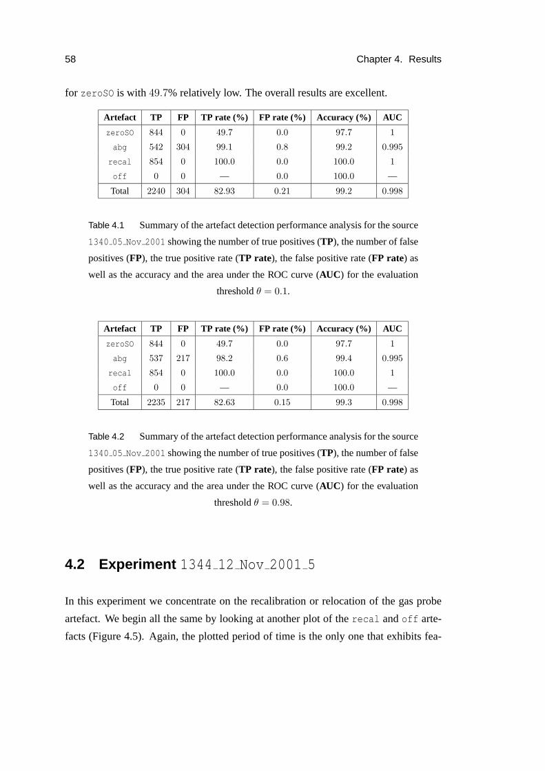
58 Chapter 4. Results
for zeroSO is with 49.7% relatively low. The overall results are excellent.
Artefact TP FP TP rate (%) FP rate (%) Accuracy (%) AUC
zeroSO 844 0 49.7 0.0 97.7 1
abg 542 304 99.1 0.8 99.2 0.995
recal 854 0 100.0 0.0 100.0 1
off 0 0 — 0.0 100.0 —
Total 2240 304 82.93 0.21 99.2 0.998
Table 4.1 Summary of the artefact detection performance analysis for the source
1340 05 Nov 2001 showing the number of true positives (TP), the number of false
positives (FP), the true positive rate (TP rate), the false positive rate (FP rate) as
well as the accuracy and the area under the ROC curve (AUC) for the evaluation
thresholdθ = 0.1.
Artefact TP FP TP rate (%) FP rate (%) Accuracy (%) AUC
zeroSO 844 0 49.7 0.0 97.7 1
abg 537 217 98.2 0.6 99.4 0.995
recal 854 0 100.0 0.0 100.0 1
off 0 0 — 0.0 100.0 —
Total 2235 217 82.63 0.15 99.3 0.998
Table 4.2 Summary of the artefact detection performance analysis for the source
1340 05 Nov 2001 showing the number of true positives (TP), the number of false
positives (FP), the true positive rate (TP rate), the false positive rate (FP rate) as
well as the accuracy and the area under the ROC curve (AUC) for the evaluation
thresholdθ = 0.98.
4.2 Experiment 1344 12 Nov 2001 5
In this experiment we concentrate on the recalibration or relocation of the gas probe
artefact. We begin all the same by looking at another plot of therecal andoff arte-
facts (Figure 4.5). Again, the plotted period of time is the only one that exhibits fea-

4.2. Experiment 1344 12 Nov 2001 5 59
0
100
200
HR [bpm]
Baby 1344, born 6 November 2001 at 12:36
0
100
200
HS [bpm]
0
50
100
SO [%]
20
30
40
TP [°C]TC [°C]
0
20
40
OX [kPa]
0
20
40
CO [kPa]
0
50
100
BS [mmHg]
0
20
40
BD [mmHg]
0
50
BM [mmHg]
0
0.5
1Recalibration
of Badger
8:57 8:58 8:59 9:00 9:01 9:02 9:03 9:04 9:05 9:06 9:07 9:08 9:09 9:10 9:11 9:12 9:130
0.5
1RecordingDevice Off
12/11/2001
Figure 4.5 This plot shows the only three interesting patterns present in source
1344 12 Nov 2001 with regard torecal andoff.
tures interesting with regard to these processes. But because off is not present at all
andrecal classifies all instances correctly, as can be seen from both,Table 4.3 and
Table 4.4, we turn to the next artefact.
So let us consider therecalGas artefact which modifies the oxygen and carbon dioxide
channels. Figure 4.6 shows its performance on the entire data set
1344 12 Nov 2001, whereas Figure 4.7 chiefly illustrates the marginal posterior prob-
abilities for the three distinct non-normal states. From the latter we can see that the
different states are modelled pretty well, party due to the fact that we constructed it
from the same source. The shown marginals also visualise what data we used to con-
struct the artefact.
Nevertheless, there was one problem withrecalGas’s marginals: At 10:28 and 10:38

60 Chapter 4. Results
0
20
40
OX [kPa]
Baby 1344, born 6 November 2001 at 12:36
0
20
40
CO [kPa]
9:00 9:30 10:00 10:30 11:00 11:30 12:00 12:30 13:00 13:30 14:00 14:30 15:00 15:30 16:00 16:30 17:00 17:30 18:00 18:300
0.5
1Recalibrationor Relocation
of OX/CO Probe
12/11/2001
Figure 4.6 Marginal posterior probabilities for the artefact process “Recalibra-
tion or relocation of the gas probe”. The high probabilities at 10:28 and 10:38 when
air is getting under the probe are the only wrong inferences made on this dataset.
0
20
40
OX [kPa]
Baby 1344, born 6 November 2001 at 12:36
0
5
10
CO [kPa]
0
0.5
1
OX 0/CO 0
0
0.5
1
OX 20/CO 5
0
0.5
1
OX high/CO low
15:16 15:18 15:20 15:22 15:24 15:26 15:28 15:30 15:32 15:34 15:36 15:38 15:400
0.5
1Recalibrationor Relocation
of OX/CO Probe
12/11/2001
Figure 4.7 Marginals for all states ofrecalGas. The inferred states visual-
ise quite exactly what data we used to construct the distinct non-normal states of
recalGas.
air is getting under the probe, which is why the probe is in fact relocated at 10:40. And
on both occasions we can observe high marginal posteriors, which is incorrect. Then
one can also spot further explaining away effects at 9:10:40and 9:12:36 due to a time

4.2. Experiment 1344 12 Nov 2001 5 61
0
100
200
HR [bpm]
Baby 1344, born 6 November 2001 at 12:36
0
200
400
BS [mmHg]
0
100
200
BD [mmHg]
0
200
400
BM [mmHg]
9:00 9:30 10:00 10:30 11:00 11:30 12:00 12:30 13:00 13:30 14:00 14:30 15:00 15:30 16:00 16:30 17:00 17:30 18:00 18:300
0.5
1
Taking BloodGas
12/11/2001
Figure 4.8 Marginal posterior probabilities of theabg artefact for the complete
source1344 12 Nov 2001. Although the number of false positives is more than
half the number of true positives (Table 4.3), the situation looks worse than itac-
tually is—especially if we recall that the CG model does not include the temporal
evolution of the signals which is fairly important in this case.
test of the recording device (compare Figure 4.5). Althoughthese effects are indeed
desirable, they negatively influences the true positive rate.
For abg the situation is worse (Figure 4.8 and Figure 4.9). Often theprocess of flush-
ing the line is characterised as drawing blood gas (10:23:20to 10:23:50 and 18:20:00
to 18:20:40 as well as 15:58 to 15:59, where the probe was additionally turned off).
Moreover, there are numerous short regions of high probability due to high blood pres-
sure values and synchronous low heart rate. The reason why the results are rather bad
is thatabg is the only modelled process that modifies HR, BS, BD and BM. There-
foreabg is quite likely to be declared responsible for any variability in those channels,
especially because the normal state is constructed in a way that results in small vari-
ances in its channel data. As we will see in the next section where we included two
further artefact processes which alter HR, BS, BD and BM,abg’s marginal posterior
probabilities become more accurate.

62 Chapter 4. Results
0
100
200
HR [bpm]
Baby 1344, born 6 November 2001 at 12:36
0
200
400
BS [mmHg]
0
100
200
BD [mmHg]
0
200
400
BM [mmHg]
10:17 10:18 10:19 10:20 10:21 10:22 10:23 10:24 10:25 10:26 10:27 10:28 10:29 10:30 10:31 10:32 10:33 10:34 10:350
0.5
1
Taking BloodGas
12/11/2001
Figure 4.9 Zoomed plot to illustrate theabg artefact, where the first region of
high probability (10:16:50 – 10:22:30) is actually corresponding to the process of
blood gas being taken, the next period starting shortly before 10:23 is caused by
flushing the line of the probe and the last spikes at 10:34 are perhaps dueto the
variability in heart rate (HR). Thus, the latter two could be misleadingly classified
as drawing blood gas.
Artefact TP FP TP rate (%) FP rate (%) Accuracy (%) AUC
zeroSO 9803 0 100.0 0.0 100.0 1
recalGas 5571 517 98.3 1.7 98.3 0.988
abg 780 530 97.9 1.5 98.5 0.989
recal 147 0 100.0 0.0 100.0 1
off 0 0 — 0.0 100.0 —
Total 16301 1047 99.03 0.64 99.4 0.994
Table 4.3 Summary of the artefact detection performance analysis for the source
1344 12 Nov 2001 showing the number of true positives (TP), the number of false
positives (FP), the true positive rate (TP rate), the false positive rate (FP rate) as
well as the accuracy and the area under the ROC curve (AUC) for the evaluation
thresholdθ = 0.1.

4.3. Experiment 1369 22 Nov 2001 7 63
Artefact TP FP TP rate (%) FP rate (%) Accuracy (%) AUC
zeroSO 9656 0 98.5 0.0 99.6 1
recalGas 5536 483 97.7 1.6 98.3 0.988
abg 770 365 96.6 1.0 98.9 0.989
recal 147 0 100.0 0.0 100.0 1
off 0 0 — 0.0 100.0 —
Total 16109 848 98.18 0.52 99.4 0.994
Table 4.4 Summary of the artefact detection performance analysis for the source
1344 12 Nov 2001 showing the number of true positives (TP), the number of false
positives (FP), the true positive rate (TP rate), the false positive rate (FP rate) as
well as the accuracy and the area under the ROC curve (AUC) for the evaluation
thresholdθ = 0.98.
The mean duration of therecalGas artefact was found to be944.8333 seconds or
15 minutes and44 seconds in this experiment. Drawing blood gas took on average
4 minutes and25 seconds, whereas the time tests of the Badger system have a mean
duration of29.4000 seconds, which is by far smaller than in our first experiment where
this procedure took exactly854 seconds. This might be an indication for two different
causes that generate the same channel values, alone with different durations; the static
CG model examined in this thesis is not able to cope with the temporal aspects of
patterns like these which is one of the limitations to be certainly addressed in the future.
4.3 Experiment 1369 22 Nov 2001 7
As we mentioned before, in this third experiment we introduce two new artefact pro-
cesses whose influence is present in the heart rate and blood pressure signals. Our
hope is that the enlarged number of artefacts whose patternsare observed on shared
physiological channels actually reduces the count of wrongly marked regions.
Before we go into more detail regarding this issue, we would briefly like to state the
major problems of the remaining artefacts. ForzeroSO, recal andoff is the situation

64 Chapter 4. Results
Artefact TP FP TP rate (%) FP rate (%) Accuracy (%) AUC
zeroSO 2565 0 95.6 0.0 99.6 1
recalGas 2797 52 99.3 0.2 99.7 1
endoSuc 86 2079 73.5 7.3 92.6 0.875
abg 180 35 87.4 0.1 99.8 0.984
recalBP 184 56 57.5 0.2 99.3 0.776
recal 117 0 99.2 0.0 100.0 0.994
off 0 0 — 0.0 100.0 —
Total 5929 2222 85.40 1.12 98.7 0.938
Table 4.5 Summary of the artefact detection performance analysis for the source
1369 22 Nov 2001 showing the number of true positives (TP), the number of false
positives (FP), the true positive rate (TP rate), the false positive rate (FP rate) as
well as the accuracy and the area under the ROC curve (AUC) for the evaluation
thresholdθ = 0.1.
still the same as in the previous experiments. That is,off is not present at all,
recal’s true positive rate is99.2% without any false positives, andzeroSO is only
suffering under explaining away issues, at least with regard to Table 4.5 and Table 4.6.
In addition to this, we would like to remark that the values inboth tables are equal for
those three artefacts, which means the marginal posterior probabilities are above0.98
for all true positives and the false negatives are all below0.1. In other words, we were
actually quite sure that the computed marginals are correct.
About the next artefact we consider,recalGas, cannot be much said either. The mar-
ginal posterior probabilities are twice very sharply peaked, before and after therecal
pattern. This is because the oxygen and carbon dioxide channels drop a little bit earlier
to zero than the remaining channels and normalise later, which results in a high prob-
ability of being in artefact state one, “OX 0/CO 0”.
Then there is also another region of high probability of the artefact being present where
it is not the case. At approximately 14:47, air is perhaps getting under the probe
leading to high oxygen pressures. These are accommodated inthe artefacts third state
which essentially models patterns of high variablilty. As arecalibration or relocation

4.3. Experiment 1369 22 Nov 2001 7 65
Artefact TP FP TP rate (%) FP rate (%) Accuracy (%) AUC
zeroSO 2565 0 95.6 0.0 99.6 1
recalGas 2772 4 98.4 0.0 99.8 1
endoSuc 79 1033 67.5 3.6 96.2 0.875
abg 98 0 47.6 0.0 99.6 0.984
recalBP 141 13 44.1 0.0 99.3 0.776
recal 117 0 99.2 0.0 100.0 0.994
off 0 0 — 0.0 100.0 —
Total 5772 1050 75.39 0.53 99.2 0.938
Table 4.6 Summary of the artefact detection performance analysis for the source
1369 22 Nov 2001 showing the number of true positives (TP), the number of false
positives (FP), the true positive rate (TP rate), the false positive rate (FP rate) as
well as the accuracy and the area under the ROC curve (AUC) for the evaluation
thresholdθ = 0.98.
of the gas probe is most likely not starting with this state, amodel which includes the
temporal evolution of the signals should be able recognise that fact.
Again, it is interesting to take a look at the tables. Now there is a difference between
the two thresholdsθ = 0.1 andθ = 0.98. In the first case, the false positive rate is
relatively high with a count of52, whereas there are only4 false positives forθ = 0.98.
Hence we were really certain that the4 false positives are predicted properly, so that
those four points might be caused by the spikes mentioned above. On the other hand,
we are not so sure about region around 14:47.
Now let us focus on the rest,endoSuc, abg andrecalBP, all of which are modelled
as modifying the same channels: HR, BS, BD and BM. From our observations in the
data, we assumed that the order of the artefacts in the previous sentence is their order in
the argument list of theconditionalGaussian class constructor, i.e.endoSuc is over-
written byabg which is itself overwritten byrecalBP.3 In addition, let us recall that
the goal of this experiment was in principle to research the interrelationship between
3The tables in this chapter do actually also indicate the order of an artefact in the poset. Upper itemsin the list are overwritten by lower ones, as in the previous chapter’s tables.

66 Chapter 4. Results
0
100
200
HR [bpm]
Baby 1369, born 21 November 2001 at 12:21
0
100
200
BS [mmHg]
0
100
200
BD [mmHg]
0
100
200
BM [mmHg]
0
0.5
1
EndotrachealSuction
0
0.5
1
Taking BloodGas
9:00 9:30 10:00 10:30 11:00 11:30 12:00 12:30 13:00 13:30 14:00 14:30 15:00 15:30 16:00 16:300
0.5
1Recalibration
of BPtransducer
22/11/2001
Figure 4.10 Marginal posterior probabilities for the artefacts endotracheal suc-
tioning, drawing blood gas and recalibrating the blood pressure transducer. Low
accuray ofendoSuc is chiefly due to a lack of specificity of the data model. See
text for details.
artefacts which alter the same channels. In particular, we hope that the introduction of
other variables thanabg might improve its accuracy, especially reducing regions where
moderately variable heart rate or blood pressure lead to wrong associations.
So let us consider one artefact and its problems after the other, starting with the drawing
of blood gas,abg. By looking at Figure 4.10, we can see that there are three blocks
with higher marginal posterior probabilities, one of which, the one in the middle, seems
to be less probable than the other two. In comparison with Figures 4.3 and 4.8 is in
this plot astonishingly few noise. This is what we were looking for.
Figure 4.11 shows the spike from 14:00 in detail. We can see that the period of time
where the marginal posterior ofabg is higher, the observed pattern does not look that
different from the typical one, as depicted in Figure 4.12. Actually, it is very likely, that

4.3. Experiment 1369 22 Nov 2001 7 67
0
100
200
HR [bpm]
Baby 1369, born 21 November 2001 at 12:21
0
100
200
BS [mmHg]
0
100
200
BD [mmHg]
0
100
200
BM [mmHg]
0
0.5
1
EndotrachealSuction
0
0.5
1
Taking BloodGas
13:59:00 13:59:30 14:00:00 14:00:30 14:01:00 14:01:30 14:02:00 14:02:30 14:03:00 14:03:30 14:04:00 14:04:300
0.5
1Recalibration
of BPtransducer
22/11/2001
Figure 4.11 Blood pressure transducer recalibration. Note the first pattern of the
marginal posteriors forabg andrecalBP in the plot. 14:04:00 to 14:04:30 might
also be flushing the line.
the observation is caused by anabg artefact. But why is pattern of the marginal pos-
terior probability now so different from the one we saw in theprevious experiments?
The answer goes as follows:
1. State “HR 0/BS low/BD high” matches the early part of theabg pattern.
2. The steadily rising pattern in BS, BD and BM which correspondsto the drawing
of blood gas, is modelled with a single state, so that this state has a mean which
lies somewhere between the top and the bottom of the pattern and the variance is
relatively large, as we estimate it from all the values, the low ones and the high
ones.
3. The explaining away effect plays a crucial part as well.

68 Chapter 4. Results
0
100
200
HR [bpm]
Baby 1369, born 21 November 2001 at 12:21
20
40
60
BS [mmHg]
20
40
60
BD [mmHg]
30
40
50
BM [mmHg]
0
0.5
1
EndotrachealSuction
0
0.5
1
Taking BloodGas
11:53:40 11:54:00 11:54:20 11:54:40 11:55:00 11:55:20 11:55:40 11:56:00 11:56:20 11:56:400
0.5
1Recalibration
of BPtransducer
22/11/2001
Figure 4.12 Typical patterns that can be observed when blood gas is being taken
from the radial arterial line and we modelled arecalBP state (“HR 0/BS low/BD
high”) similar to the beginning of pattern (11:54 – 11:55).
As a result, the early stage of drawing blood gas is actually more likely to be arecalBP
event due to the way we constructed their state data. But the more the blood pressures
rise, the more likely isabg’s responsiblilty for having generated this pattern and the
explaining away effect therefore starts to diminishrecalBP’s marginal posterior prob-
ability.
This means thatrecalBP is classified wrongly asabg approximately as often asabg
is asrecalBP. Table 4.5 and Table 4.6 reflect these findings at least partially. So is for
exampleabg’s true positive rate forθ = 0.1 87.4%, whereas it is only47.6 in the other
case, when we are cutting marginals close to their top.
Finally, let us say some words about theendoSuc artefact. First of all, it is clear
that the marginals shown in Figure 4.10 do not look very nice and neither do the error
statistics. But the main problem when modelling endotracheal suctionings is the lack of

4.4. Experiment 1355 14 Nov 2001 8 69
a temporal model, since the only clear indication is a small drop in heart rate for about
half a minute, which also renders the collection of adequatesamples more problematic.
Usually there are also some related effects on the blood pressures takeing place, on a
larger time scale though. In this experiment we modelled theendoSuc artefact with
two different non-normal states; the first as the short HR drop and the second as its
effect on BS, BD and BM, which is an increase.
Because of the lack of specificity, this artefact takes on the role of a “garbage collector”.
This becomes particularly apparent from circa 15:30 – 16:33.
The mean durations we computed for this experiment are as follows:
recalGas: 939 seconds= 15 minutes and39 seconds
endoSuc: 39 seconds (without aftereffects)4
abg: 103 seconds= 1 minute and43 seconds
recalBP: 320 seconds= 5 minutes and20 seconds
4.4 Experiment 1355 14 Nov 2001 8
In this experiment there is not really something we haven’t encountered before apart
from an additional channel, the respiratory rate RR, and therefore we will not spend
to much time on it. Since the only interesting artefact pattern we were able to identify
in conjunction with this channel are the drop outs to zero, the other artefact models
stay primarily the same.abg andrecalBP, however, had to be changed as they do not
modify the HR channel in this source data set. As a consequence, we also introduced
an artefact model for heart rate drop outs to zero, calledzeroHR. We begin by stating
that all artefacts which model drop outs on a single channel,i.e.zeroSO, zeroRR and
zeroHR, do their job extraordinarily well (Figure 4.13)—which is not really amazing
since one could also find them deterministically. Thus, whenconsidering cross product
state space reductions, the removal of those easy to preprocess artefacts should be
4We also evaluated theendoSuc artefact without including the aftereffects, which partially explainsthe bad AUC values et cetera.

70 Chapter 4. Results
0
100
200
HR [bpm]
Baby 1355, born 12 November 2001 at 17:17
100
150
200
HS [bpm]
60
80
100
SO [%]
0
100
200
RR [1/min]
0
0.5
1
Zero SO / HS
0
0.5
1
Zero RR
16:44:00 16:44:20 16:44:40 16:45:00 16:45:20 16:45:40 16:46:00 16:46:20 16:46:40 16:47:00 16:47:20 16:47:40 16:48:000
0.5
1
Zero HR
14/11/2001
Figure 4.13 Example of zero drop outs in HR and RR. The SO signal seemed to
be measured reliably in source1355 14 Nov 2001. As one can see, the marginal
posterior probabilities model the drop outs well which is not really astonishing.
preferred over other more complex ones. From Table 4.7 and Table 4.8 we see the
accuracy is at least99.7%, while the true positive rate ofzeroHR is only 42.1%, of
zeroSO even0. The latter, in combination with the accuracy, means that there are
only a few points where the SO value plummets to zero and we were certain about
their categorisation as not beingzeroSO artefacts. Similarly, less than half of the
observations with zeros in HR are regarded as being a consequence ofzeroHR being
present, which is due to the recalibration of the recording device, as can be seen from
the following simple calculation: 5656+74
≈ 43.1%.
From 11:13 on for about one hour air seem to be getting under the combined oxy-
gen/carbon dioxide probe, which is again wrongly categorised as being caused by
recalGas which is apparently not true. Figure 4.14 shows one of those misinterpreta-
tion as being modelled as the “OX high/CO low” state ofrecalGas. A model which
would take care of the temporal evolution should be able to get rid of those misinter-

4.4. Experiment 1355 14 Nov 2001 8 71
0
20
40
OX [kPa]
Baby 1355, born 12 November 2001 at 17:17
0
10
20
CO [kPa]
0
0.5
1
OX 0/CO 0
0
0.5
1
OX 20/CO 5
0
0.5
1
OX high/CO low
11:40 11:50 12:00 12:10 12:20 12:30 12:40 12:50 13:00 13:100
0.5
1
Recalibrationor Relocation
of OX/CO Probe
14/11/2001
Figure 4.14 Plot of the marginal posterior probabilities for all states of arte-
fact recalGas. The real cause of the misleadingly high probabilities of state “OX
high/CO low” at 11:50 is most probably due to air getting under the probe.
pretations as therecalGas artefact usually starts in the “OX 0/CO 0” state, as can be
seen from the second half of the previously mentioned figure.Moreover, it should be
remarked that the false positives ofrecalGas differ dramatically for the two different
thresholds without changing the true positive rate a lot.
Figure 4.15 presents an overview of the marginal posterior probabilities for theabg
andrecalBP artefacts. Apart from the periods of time where blood gas hasreally
been taken (9:05, 13:16 and 16:11), the causes of the patterns which have misleadingly
caused theabg’s marginal posteriors to be high are given below:
11:42:30 is an unknown artefact;
14:42 – 14:43 is maybe due to emptying water from ventilator trap;
16:21:55 and 16:23:15 seem to be problems with adapting to high or low blood pres-

72 Chapter 4. Results
0
100
200
HR [bpm]
Baby 1355, born 12 November 2001 at 17:17
0
50
100
BS [mmHg]
0
50
100
BD [mmHg]
0
50
100
BM [mmHg]
0
0.5
1
Taking BloodGas
8:30 9:00 9:30 10:00 10:30 11:00 11:30 12:00 12:30 13:00 13:30 14:00 14:30 15:00 15:30 16:00 16:30 17:00 17:30 18:000
0.5
1
Recalibrationof BP
transducer
14/11/2001
Figure 4.15 Overview of the marginal posteriors for the artefactsabg and
recalBP. EspeciallyrecalBP’s model seems to work rather fine here.
sures in conjunction withrecalBP (its “high/high” or “low/low” states are caught
by abg as illustrated in Figure 4.16);
17:01 – 17:06 is an unknown artefact;
17:27 – 17:39 is another unknown artefact;
18:09 – 18:23 is unknown as well.
TherecalBP artefact reveals only two very short periods of slightly higher marginal
posterior probabilities (approximately0.6), the second of which is shown more clearly
in the first quarter of Figure 4.16.
Finally, there is a one second drop at 10:24:56 where almost all channels (including the
temperatures) plummet to zero. But because the carbon dioxide (CO) value is normal,
this is correctly recognised as not being anoff artefact. Nonetheless, we certainly
could integrate drop outs as the one above in a new multinomial variable, together

4.5. Experiment 1369 21 Nov 2001 9 73
140
160
180
HR [bpm]
Baby 1355, born 12 November 2001 at 17:17
0
50
100
BS [mmHg]
0
50
100
BD [mmHg]
0
50
100
BM [mmHg]
0
0.5
1
Taking BloodGas
16:09 16:10 16:11 16:12 16:13 16:14 16:15 16:16 16:17 16:18 16:19 16:20 16:21 16:22 16:23 16:240
0.5
1
Recalibrationof BP
transducer
14/11/2001
Figure 4.16 Detail of the marginals in Figure 4.15.
with recal’s non-normal states as discussed in subsection 3.2.3.
The mean durations for experiment1355 14 Nov 2001 8 are:
recalGas: 1364.7 seconds= 22 minutes and44 seconds
abg: 181 seconds= 3 minutes and1 second
recalBP: 95 seconds= 1 minute and35 seconds
4.5 Experiment 1369 21 Nov 2001 9
The absence of theoff artefact in the last four experiments certainly leads to theques-
tion why we need to have it at all. In this experiment we demonstrate its usefulness.
Furthermore, and in fact in conjunction with theoff artefact we present a clear ex-
ample of the effects the explaining away phenomenon has on various channels, con-

74 Chapter 4. Results
Artefact TP FP TP rate (%) FP rate (%) Accuracy (%) AUC
zeroSO 0 0 0.0 0.0 99.8 0.971
zeroRR 2267 0 96.6 0.0 99.8 0.999
zeroHR 56 0 42.1 0.0 99.8 0.983
recalGas 4023 718 98.3 2.2 97.8 0.996
abg 539 1824 99.3 5.1 94.9 0.994
recalBP 92 6 96.8 0.0 100.0 0.986
recal 74 0 97.4 0.0 100.0 0.98
off 0 0 — 0.0 100.0 —
Total 7051 2548 75.77 0.92 99.0 0.987
Table 4.7 Summary of the artefact detection performance analysis for the source
1355 14 Nov 2001 showing the number of true positives (TP), the number of false
positives (FP), the true positive rate (TP rate), the false positive rate (FP rate) as
well as the accuracy and the area under the ROC curve (AUC) for the evaluation
thresholdθ = 0.1.
Artefact TP FP TP rate (%) FP rate (%) Accuracy (%) AUC
zeroSO 0 0 0.0 0.0 99.8 0.971
zeroRR 2235 0 95.2 0.0 99.7 0.999
zeroHR 56 0 42.1 0.0 99.8 0.983
recalGas 4001 39 97.7 0.1 99.6 0.996
abg 487 315 89.7 0.9 99.0 0.994
recalBP 92 2 96.8 0.0 100.0 0.986
recal 74 0 97.4 0.0 100.0 0.98
off 0 0 — 0.0 100.0 —
Total 6945 356 74.13 0.13 99.7 0.987
Table 4.8 Summary of the artefact detection performance analysis for the source
1355 14 Nov 2001 showing the number of true positives (TP), the number of false
positives (FP), the true positive rate (TP rate), the false positive rate (FP rate) as
well as the accuracy and the area under the ROC curve (AUC) for the evaluation
thresholdθ = 0.98.

4.5. Experiment 1369 21 Nov 2001 9 75
Artefact TP FP TP rate (%) FP rate (%) Accuracy (%) AUC
zeroSO 4111 0 100.0 0.0 100.0 1
zeroHR 2907 523 87.6 2.4 96.3 0.961
zeroRR 4168 2 99.9 0.0 100.0 1
recalGas 11699 1883 95.9 14.6 90.5 0.986
endoSuc 140 2497 51.7 10.1 89.5 0.791
abg 815 411 69.8 1.7 97.0 0.897
recalBP 14 3461 82.4 13.8 86.2 0.85
recal 40 3 100.0 0.0 100.0 1
off 1515 0 100.0 0.0 100.0 1
Total 25409 8780 87.46 4.74 95.5 0.943
Table 4.9 Summary of the artefact detection performance analysis for the source
1369 21 Nov 2001 showing the number of true positives (TP), the number of false
positives (FP), the true positive rate (TP rate), the false positive rate (FP rate) as
well as the accuracy and the area under the ROC curve (AUC) for the evaluation
thresholdθ = 0.1.
centrating on the drop outs to zero in HR, RR and SO. We also give further examples
for abg andrecalBP. In subsection 3.4.5 we stated thatrecalBP are modelled on BD,
BS and BM only, whereasabg andendoSuc are constructed using HR as well. What
is more is thatendoSuc has been modified to include one non-normal state only, the
one which corresponds to small bowl-shaped drops in heart rate. The second state that
was meant to take the aftereffects of this decrease in HR intoconsideration has thence
been removed. Altogether, our model comprises nine distinct artefacts.
We begin our discussion of experiment1369 21 Nov 2001 9 with off and recal.
First, and maybe most important, we note that both have been classified perfectly, even
for θ = 0.98, as can be seen from Table 4.5, Table 4.6 and also from Figure 4.17.
Second, as Figure 4.17 shows, we observe thatoff infers the zero values correctly
from 12:22 onward to circa 12:47, the time the first channel’ssignal takes on a non-
zero value. Unfortunately, the different channels do not return to normal at the same
time. This has major implications for the classification measures we provide, since
all of the zero values prior to the first normal ones have been included into the labels

76 Chapter 4. Results
Artefact TP FP TP rate (%) FP rate (%) Accuracy (%) AUC
zeroSO 2556 0 62.1 0.0 93.8 1
zeroHR 532 13 16.0 0.1 88.8 0.961
zeroRR 2601 0 62.4 0.0 93.7 1
recalGas 10923 192 89.6 1.5 94.2 0.986
endoSuc 36 331 13.3 1.3 97.7 0.791
abg 656 59 56.2 0.2 97.7 0.897
recalBP 14 3461 82.4 13.8 86.2 0.85
recal 40 3 100.0 0.0 100.0 1
off 1515 0 100.0 0.0 100.0 1
Total 18873 4059 64.66 1.88 94.7 0.943
Table 4.10 Summary of the artefact detection performance analysis for the
source1369 21 Nov 2001 showing the number of true positives (TP), the num-
ber of false positives (FP), the true positive rate (TP rate), the false positive rate
(FP rate) as well as the accuracy and the area under the ROC curve (AUC) for the
evaluation thresholdθ = 0.98.
which help to determine those measures. Take a look at Figure4.18. Here we can
clearly see the effect of howoff andrecal reduce the marginal posterior probabilities
of other artefacts, i.e. how they render them unlikely. What can hardly be seen from
Figure 4.18, is thatzeroHR is below theθ = 0.1 threshold for the periodoff is inferred
to be present. This becomes obvious when comparing Table 4.5and Table 4.6. In
the first table,zeroHR exhibits a by far larger number of false positives thanzeroSO
or zeroRR, whereas in the second table, forθ = 0.98, the false positive counts are
certainly more similar. This means that the difference in accuracy, but not in AUC, is
chiefly a consequence ofzeroHR’s marginal posterior probability being greater then
θ = 0.1 whenoff is present. There is also an immense difference between the true
positives of both,zeroHR andzeroSO/zeroRR as well as between the two thresholds
θ = 0.1 andθ = 0.98. For example, forθ = 0.1 the true positive rate is87.6%, more
than five times the rate forθ = 0.98. We believe that this is mainly a consequence
of theabg artefact explaining parts ofzeroHR’s responsibilies away. And we will see
below that the contrary is true as well. Therefore the numberof artefacts that alter the

4.5. Experiment 1369 21 Nov 2001 9 77
0200400
HR [bpm]
Baby 1369, born 21 November 2001 at 12:21
0200400
HS [bpm]
050
100
SO [%]
0100200
RR [1/min]
02040
TC [°C]TP [°C]
02040
OX [kPa]
05
10
CO [kPa]
00.5
1
BS [mmHg]
00.5
1
BD [mmHg]
00.5
1
BM [mmHg]
00.5
1Recalibration
of Badger
12:44 12:46 12:48 12:50 12:52 12:54 12:56 12:58 13:00 13:02 13:04 13:060
0.51
RecordingDevice Off
21/11/2001
Figure 4.17 This plot shows the marginal posterior probabilities for the artefacts
off andrecal. The latter differs from the first only be the fact that the temperatures
are20 Celsius and not0.
same channels in similar ways tend to interact greatly.
Next we considerrecalGas in brief. Although not illustrated, there was only one
explicit problem between 15:08 and 15:09, where the CO channel is zero and OX
values are high pressures (9 to 12 kPa). Its real cause is unknown. In addition, the
artefact pattern from 16:27 – 17:20 is probably no relocation of the gas probe, although
one might infer this from the observations; but it is known that the incubator was
open and the annotations in TSW are in favour of the peripheral venous line being
removed/inserted.
Figure 4.19 visualises the marginal posterior probabilities for the three artefactsendoSuc,
abg andrecalBP. This time we start with therecalBP, which is at least in this exper-
iment the wrong name for the patterns we modelled. A better label would be “Start up

78 Chapter 4. Results
0
200
400
HR [bpm]
Baby 1369, born 21 November 2001 at 12:21
0
200
400
HS [bpm]
0
50
100
SO [%]
0
100
200
RR [1/min]
0
0.5
1
Zero SO / HS
0
0.5
1
Zero HR
12:42 12:44 12:46 12:48 12:50 12:52 12:54 12:56 12:58 13:00 13:02 13:04 13:060
0.5
1
Zero RR
21/11/2001
Figure 4.18 This is a clear example of how one artefact’s presence (off from
12:42 – 12:47 and actuallyrecal as well around 13:05) changes another one’s
marginal posterior probability (zeroSO, zeroHR andzeroRR). This effect is com-
monly referred to as “explaining away”.
of the blood pressure transducer” or something similar. Itsstates are reduced to two,
one where the blood pressures are kind of maximal and one where they are zero. Thus
there should not be an interaction withabg and the period of zero values in whichoff
is absent, leads to the given values in Tables 4.9 and 4.10. The latter is also shown in
Figure 4.19, whereas Figure 4.20 indicates the first. Overall, the true positive rates are
rather high (82.4%) because of the specificity of the model.
Now if there is no interaction betweenrecalBP andabg, why can we observe the
typical pattern in Figure 4.20, from 17:30 to 17:31? Recalling thatzeroHR is part of
the current model, we are in the position to explain this pattern. As HR is obviously
a good indicator for bothzeroHR andabg, the only evidence on which the outcoming
marginals might be based are the blood pressure values. And this is exactly what is
depicted in Figure 4.20
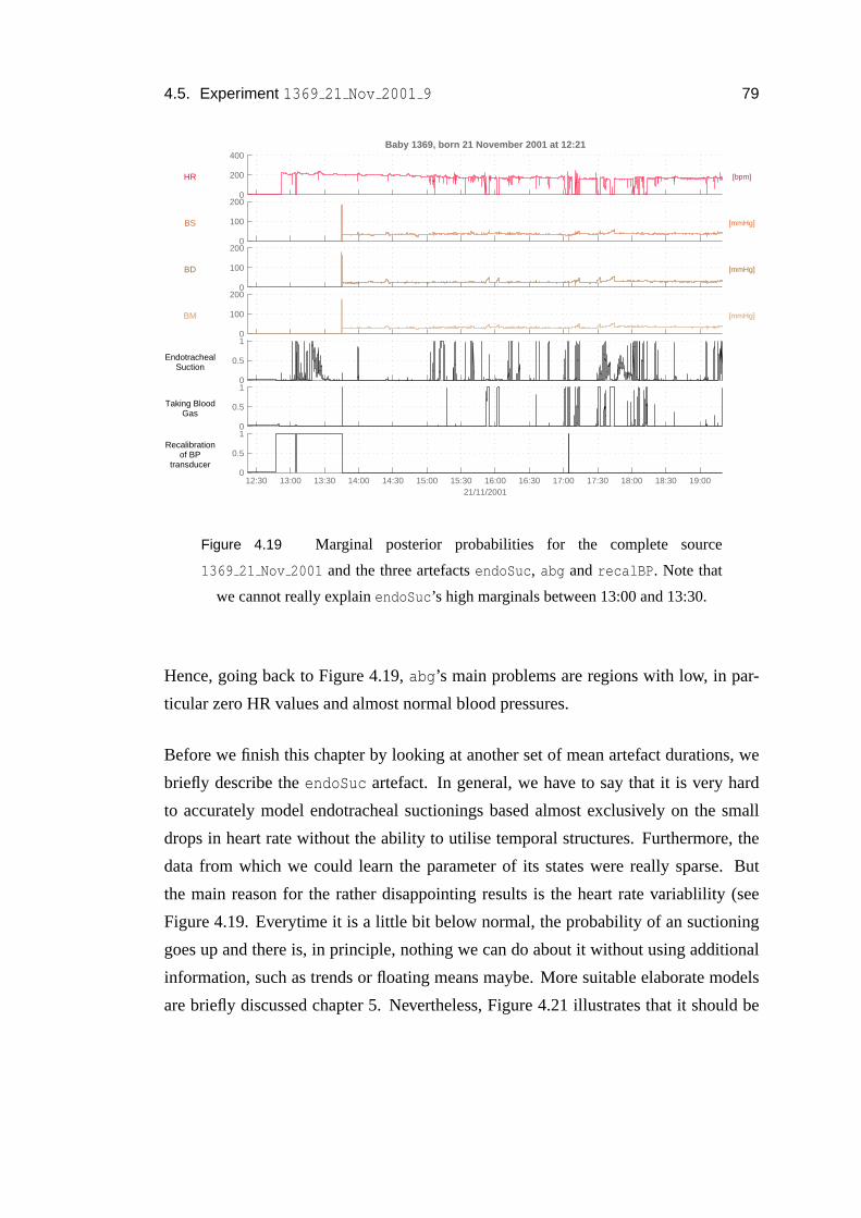
4.5. Experiment 1369 21 Nov 2001 9 79
0
200
400
HR [bpm]
Baby 1369, born 21 November 2001 at 12:21
0
100
200
BS [mmHg]
0
100
200
BD [mmHg]
0
100
200
BM [mmHg]
0
0.5
1
EndotrachealSuction
0
0.5
1
Taking BloodGas
12:30 13:00 13:30 14:00 14:30 15:00 15:30 16:00 16:30 17:00 17:30 18:00 18:30 19:000
0.5
1Recalibration
of BPtransducer
21/11/2001
Figure 4.19 Marginal posterior probabilities for the complete source
1369 21 Nov 2001 and the three artefactsendoSuc, abg andrecalBP. Note that
we cannot really explainendoSuc’s high marginals between 13:00 and 13:30.
Hence, going back to Figure 4.19,abg’s main problems are regions with low, in par-
ticular zero HR values and almost normal blood pressures.
Before we finish this chapter by looking at another set of mean artefact durations, we
briefly describe theendoSuc artefact. In general, we have to say that it is very hard
to accurately model endotracheal suctionings based almostexclusively on the small
drops in heart rate without the ability to utilise temporal structures. Furthermore, the
data from which we could learn the parameter of its states were really sparse. But
the main reason for the rather disappointing results is the heart rate variablility (see
Figure 4.19. Everytime it is a little bit below normal, the probability of an suctioning
goes up and there is, in principle, nothing we can do about it without using additional
information, such as trends or floating means maybe. More suitable elaborate models
are briefly discussed chapter 5. Nevertheless, Figure 4.21 illustrates that it should be

80 Chapter 4. Results
0
200
400
HR [bpm]
Baby 1369, born 21 November 2001 at 12:21
20
40
60
BS [mmHg]
20
40
60
BD [mmHg]
20
40
60
BM [mmHg]
0
0.5
1
EndotrachealSuction
0
0.5
1
Taking BloodGas
17:29 17:30 17:31 17:32 17:33 17:34 17:35 17:36 17:37 17:38 17:39 17:40 17:41 17:42 17:43 17:44 17:45 17:460
0.5
1Recalibration
of BPtransducer
21/11/2001
Figure 4.20 Another example of the explaining away phenomenon. The steady
rise in the first marginal posterior ofabg is this time not caused byrecalBP as can
be seen from its own marginal posterior probability, but byzeroHR which “com-
petes” withabg on HR.
possible to recognise this artefact more effectively.
And here are some mean artefact durations as calculated from1369 21 Nov 2001:
recalGas: 3048.3 seconds= 50 minutes and48 seconds
endoSuc: 38.7 seconds
abg: 233.6 seconds= 3 minutes and53 seconds
recalBP: 8.5 seconds
recal: 20 seconds

4.5. Experiment 1369 21 Nov 2001 9 81
0
100
200
HR [bpm]
Baby 1369, born 21 November 2001 at 12:21
30
40
50
BS [mmHg]
20
30
40
BD [mmHg]
20
30
40
BM [mmHg]
0
0.5
1
EndotrachealSuction
0
0.5
1
Taking BloodGas
16:10:30 16:11:00 16:11:30 16:12:00 16:12:30 16:13:00 16:13:30 16:14:00 16:14:30 16:15:00 16:15:300
0.5
1Recalibration
of BPtransducer
21/11/2001
Figure 4.21 Example of an endotracheal suctioning.


Chapter 5
Conclusions and Future Work
This chapter asks what conclusions we can draw from the material covered in the
preceding chapters and makes suggestions for future work, including enhancements to
our approach of using a conditional Gaussian model to detectartefacts in the neonatal
monitoring data.
5.1 Conclusions
In this thesis we aimed to detect artefact processes in neonatal monitoring data using a
probabilistic approach, the conditional Gaussian (CG) model. And although our results
are actually promising, this model has to be seen as the first part of the construction of
a more elaborate model—one that includes the temporal aspects of the data.
This is, to the best of our knowledge, the first approach whichtries to infer multiple
latent causes from patient monitoring data. And the resultspresented in chapter 4
underpin the fact that this goal has been accomplished. It is, of course, true that there
are still several problems that need to be addressed in future; but the recognition of
artefactual patterns in multi-channel data is feasible.
We devoted a large amount of the allotted time on solving datamining and prepro-
cessing tasks as well as on the creation of a comfortable computing environment within
83

84 Chapter 5. Conclusions and Future Work
MATLAB . Now we are in the position to build new instances of the CG models fast
and accurately.
Moreover, we gave an algorithm which dramatically reduces the cross product state
space of the latent variables by exploiting the structure ofartefacts. This is useful not
only while we are learning the parameters of the CG distribution, but also when we
compute posterior or marginal posterior probabilities. Inhow far this algorithm will
be useful in conjunction with models that acknowledge the temporal evolution of the
recorded signals, still needs to be seen.
Perhaps most significantly, we have shown that the conditional Gaussian model is a
valid approach to the detection of multiple hidden causes inthe data. The application
of this model on the other hand, helped us understand the interactions between the
various artefact processes themselves.
5.2 Future work
Simple enhancements of this work include the generalisation of the software we cre-
ated, so that, for instance, evidence can be entered into thebelief network or annota-
tions can be stored. We could also modify the current software tools to create labels
sufficient for automatic estimation of parameters, say.
More important, however, would be the implementation of theproposed algorithm to
reduce the cross product state space and thus increase the number of useable artefacts
and speed up the inference of their states.
We might also benefit from computing more detailed data statistics such as the physiolo-
gical centiles collected by Neil McIntosh. Especially in the light of modelling the
baby’s normal state of health it might be wise to know more about the distributions
of the individual channels, or subsets of them. Then we coulddecide with a lot more
confidence on how to model the observations. We might even want to have some kind
of artefact process inventory in the long run.
In every case it is necessary to have access to data with labels that can be directly

5.2. Future work 85
applied in the machine learning context. The absence of these labels made the con-
struction as well as the evaluation of the model so much more difficult.
Furthermore, it is our opinion that there is still a lot to be learned from the everyday
procedures within an ICU and a detailed knowledge about the processes at the cot-side
would certainly facilitate the construction of other artefacts.
In addition to this, we have to include preprocessing techniques as the ones discussed in
section 1.2. The pattern matching approach based on piecewise linear segmentations
(Keogh et al. (2003); Keogh and Smyth (1997)) of the channel data did not really
work, however. Maybe the usage of autoregressive hidden Markov models (Penny and
Roberts (1999); Woodland (1992)) would be a reasonable approach. But a lot simpler
could be the exploitation of the fact that systolic and diastolic blood pressure become
the same when the nurse is drawing blood gas. Simple tests showed that this method
could be a sensible extension to the current system.
Finally, and certainly most significantly, we have to include temporal aspects into our
models. That is, we have to replicate the CG model through time. The result of this
operation would be a factorial hidden Markov model (FHMM) with conditional Gaus-
sian observation model instead of a conditional linear Gaussian one as described in
Ghahramani and Jordan (1997).
Do our results regarding the cross product state space reduction carry over to FHMMs?


Appendix A
Additional plots
In this appendix we gathered some plots which might be interesting to the reader,
although they are not particularly relevant to the understanding of our approach. We
present histograms for the channels available in the data sources as well as plots of the
entire data for the five experiments carried out.
87

88 Appendix A. Additional plots
0 50 100 150 200 2500
0.5
1
1.5
2
2.5
3
3.5x 10
4 HR
[bpm]
Figure A.1 Histogram for channel HR.
0 50 100 150 200 2500
0.5
1
1.5
2
2.5
3
3.5
4
4.5x 10
4 HS
[bpm]
Figure A.2 Histogram for channel HS.

89
0 5 10 15 20 25 30 35 40 450
2
4
6
8
10
12
14x 10
4 TC
[°C]
Figure A.3 Histogram for channel TC.
0 20 400
1
2
3
4
5
6
7
8
9
10x 10
4 TP
[°C]
Figure A.4 Histogram for channel TP.

90 Appendix A. Additional plots
0 5 10 15 20 25 300
1
2
3
4
5
6
7
8x 10
4 OX
[kPa]
Figure A.5 Histogram for channel OX.
0 5 10 15 20 25 300
1
2
3
4
5
6
7
8
9x 10
4 CO
[kPa]
Figure A.6 Histogram for channel CO.

91
0 50 100 150 200 250 3000
1
2
3
4
5
6
7
8
9x 10
4 BS
[mmHg]
Figure A.7 Histogram for channel BS.
0 20 40 60 80 100 120 140 160 180 2000
1
2
3
4
5
6
7
8
9x 10
4 BD
[mmHg]
Figure A.8 Histogram for channel BD.

92 Appendix A. Additional plots
0 50 100 150 200 2500
1
2
3
4
5
6
7
8
9x 10
4 BM
[mmHg]
Figure A.9 Histogram for channel BM.
0 10 20 30 40 50 60 70 80 90 1000
0.5
1
1.5
2
2.5
3
3.5
4
4.5x 10
4 SO
[%]
Figure A.10 Histogram for channel SO.

93
−20 0 20 40 60 80 100 120 140 1600
0.5
1
1.5
2
2.5x 10
5 RR
[1/min]
Figure A.11 Histogram for channel RR.

94A
ppendixA
.A
dditionalplots
0
100
200
HR [bpm]
Baby 1340, born 4 November 2001 at 14:27
0
100
200
HS [bpm]
0
50
100
SO [%]
20
30
40
TP [°C]TC [°C]
0
50
100
BS [mmHg]
0
50
100
BD [mmHg]
9:00 9:30 10:00 10:30 11:00 11:30 12:00 12:30 13:00 13:30 14:00 14:30 15:00 15:30 16:00 16:30 17:00 17:30 18:00 18:300
50
100
BM [mmHg]
05/11/2001
Figure
A.12
Source1340
05Nov
2001.

95
0
100
200
HR [bpm]
Baby 1344, born 6 November 2001 at 12:36
0
100
200
HS [bpm]
0
50
100
SO [%]
20
30
40
TP [°C]TC [°C]
0
20
40
OX [kPa]
0
20
40
CO [kPa]
0
200
400
BS [mmHg]
0
100
200
BD [mmHg]
9:00 9:30 10:00 10:30 11:00 11:30 12:00 12:30 13:00 13:30 14:00 14:30 15:00 15:30 16:00 16:30 17:00 17:30 18:00 18:300
200
400
BM [mmHg]
12/11/2001
Figure
A.13
Source1344
12Nov
2001.

96A
ppendixA
.A
dditionalplots
0
100
200
HR [bpm]
Baby 1369, born 21 November 2001 at 12:21
0
100
200
HS [bpm]
0
50
100
SO [%]
20
30
40
TP [°C]TC [°C]
0
20
40
OX [kPa]
0
5
10
CO [kPa]
0
100
200
BS [mmHg]
0
100
200
BD [mmHg]
9:00 9:30 10:00 10:30 11:00 11:30 12:00 12:30 13:00 13:30 14:00 14:30 15:00 15:30 16:00 16:300
100
200
BM [mmHg]
22/11/2001
Figure
A.14
Source1369
22Nov
2001.

97
0
100
200
HR [bpm]
Baby 1355, born 12 November 2001 at 17:17
0
100
200
HS [bpm]
0
50
100
SO [%]
0
20
40
TP [°C]TC [°C]
0
20
40
OX [kPa]
0
10
20
CO [kPa]
0
50
100
BS [mmHg]
0
50
100
BD [mmHg]
0
50
100
BM [mmHg]
8:30 9:00 9:30 10:00 10:30 11:00 11:30 12:00 12:30 13:00 13:30 14:00 14:30 15:00 15:30 16:00 16:30 17:00 17:30 18:000
100
200
RR [1/min]
14/11/2001
Figure
A.15
Source1355
14Nov
2001.

98A
ppendixA
.A
dditionalplots
0
200
400
HR [bpm]
Baby 1369, born 21 November 2001 at 12:21
0
200
400
HS [bpm]
0
50
100
SO [%]
0
20
40
TC [°C]TP [°C]
0
20
40
OX [kPa]
0
20
40
CO [kPa]
0
100
200
BS [mmHg]
0
100
200
BD [mmHg]
0
100
200
BM [mmHg]
12:30 13:00 13:30 14:00 14:30 15:00 15:30 16:00 16:30 17:00 17:30 18:00 18:30 19:000
100
200
RR [1/min]
21/11/2001
Figure
A.16
Source1369
21Nov
2001.

Bibliography
Alberdi, E., Becher, J.-C., Gilhooly, K., Hunter, J. R. W., Logie, R., Lyon, A.,
McIntosh, N., and Reiss, J. (2001). Expertise and the interpretation of compu-
terized physiological data: Implications for the design ofcomputerized monitor-
ing in neonatal intensive care.International Journal of Human Computer Studies,
55(3):191–216.
Becker, K., Thull, B., Kasmacher-Leidinger, H., Stemmer, J., Rau, G., Kalff, G., and
Zimmermann, H.-J. (1997). Design and vaildation of an intelligent patient monitor-
ing and alarm system based on a fuzzy logic process model.Artificial Intelligence
in Medicine, 11:33–53.
Bishop, C. M. (1995).Neural Networks for Pattern Recognition. Oxford University
Press, Oxford, UK.
Cao, C. and McIntosh, N. (1998). Empirical study on artifact detection in monitoring
data. Informatics Program, Children’s Hospital, 310 Longwood Avenue, Boston,
USA.
Cao, C. and McIntosh, N. (2000). An event-based approach to identifying artifacts in
multiple channel monitoring data from preterm infants. Technical report, Depart-
ment of Child Life and Health, University of Edinburgh.
Ghahramani, Z. and Jordan, M. I. (1997). Factorial hidden Markov models.Machine
Learning, 29:245–273.
Haimowitz, I. J., Le, P. P., and Kohane, I. S. (1995). Clinicalmonitoring using
regression-based trend templates.Artificial Intelligence in Medicine, 7(6):473–496.
99

100 BIBLIOGRAPHY
Hand, D., Mannila, H., and Smyth, P. (2001).Principles of Data Mining. Adaptive
Computation and Machine Learning. The MIT Press, Cambridge, USA.
Hanley, J. A. and McNeil, B. J. (1982). The meaning and use of the area under a
Receiver Operating Characteristic (ROC) curve.Radiology, 143(1):29–36.
Hoare, S. W., Asbridge, D., and Beatty, P. C. W. (2002). On-linenovelty detection for
artefact identification in automatic anaesthesia record keeping.Medical Engineering
& Physics, 24:673–681.
Hoare, S. W. and Beatty, P. C. W. (2000). Automatic artifact identification in anaes-
thesia patient record keeping: a comparison of techniques.Medical Engineering &
Physics, 22:547–553.
Hunter, J. (2001).Time Series Workbench: User’s Manual. Department of Computing
Science, University of Aberdeen.
Jordan, M. I. (2002). An introduction to probabilistic graphical models. Unpublished
manuscript.
Keogh, E., Chu, S., Hart, D., and Pazzani, M. (2003).Data Mining in Time Series
Databases, chapter Segmenting Time Series: A Survey and Novel Approach. World
Scientific Publishing Company.
Keogh, E. and Smyth, P. (1997). A probabilistic approach to fast pattern matching
in time series databases. In Heckerman, D., Mannila, H., Pregibon, D., and Uthur-
usamy, R., editors,Third International Conference on Knowledge Discovery and
Data Mining, pages 24–30, Newport Beach, CA, USA. AAAI Press, Menlo Park,
California.
Koski, E. M. J., Makivirta, A., Sukuvaara, T., and Kari, A. (1990). Frequencyand re-
liability of alarms in the monitoring of cardiac postoperative patients.International
Journal of Clinical Monitoring and Computing, 7:129–133.
Lauritzen, S. L. and Jensen, F. (1999). Stable local computation with conditional
gaussian distributions. Technical Report R-99-2014, Department of Mathematical
Sciences, Aalborg University.

BIBLIOGRAPHY 101
Lauritzen, S. L. and Wermuth, N. (1984). Mixed interaction models. Technical Report
R-84-8, Institute for Electronic Systems, Aalborg University.
Lauritzen, S. L. and Wermuth, N. (1989). Graphical models for associations between
variables, some of which are qualitative and some quantitative. In Annals of Statist-
ics, volume 17, pages 31–57.
Lawless, S. T. (1994). Crying wolf: false alarms in the pediatric intensive care unit.
Critical Care Medicine, 22:981–985.
McIntosh, N. (2002). Intensive care monitoring: past, present and future.Clinical
Medicine, 2(4):349–355.
Meredith, C. and Edworthy, J. (1995). Are there too many alarms in the intensive care
unit? An overview of the problems.Journal of Advanced Nursing, 21:15–20.
Miksch, S., Horn, W., Popow, C., and Paky, F. (1996). Utilizing temporal data ab-
straction for data validation and therapy planning for artificially ventilated newborn
infants.Artificial Intelligence in Medicine, 8(6):543–576.
Pearl, J. (1988).Probabilistic reasoning in inteligent systems: Networks of plausible
inference. Morgan Kaufmann, San Mateo, USA.
Penny, W. and Roberts, S. (1999). Dynamic models for nonstationary signal segment-
ation. Computers and Biomedical Research, 32(6):483–502.
Smyth, P. (1994a). Hidden Markov models for fault detectionin dynamic systems.
Pattern Recognition, 27(1):149–164.
Smyth, P. (1994b). Markov monitoring with unknown states.IEEE Journal on Selected
Areas in Communications (JSAC), Special Issue on IntelligentSignal Processing for
Communications.
The MathWorks, Inc. (2003). MATLAB . Natick, USA.
http://www.mathworks.com/products/matlab/.
Tipping, M. (1999). Statistical pattern analysis. Unpublished manuscript.
Tsien, C. L. (2000a). Event discovery in medical time-seriesdata. InAMIA 2000
102 BIBLIOGRAPHY
Annual Symposium, pages 858–862. American Medical Informatics Association
(AMIA).
Tsien, C. L. (2000b).TrendFinder: Automated Detection of Alarmable Trends. PhD
thesis, Department of Electrical Engineering and Computer Science, Massachussetts
Institute of Technology, Cambridge, USA.
Tsien, C. L. and Fackler, J. C. (1997). Poor prognosis for existing monitors in the
intensive care unit.Critical Care Medicine, 25(4):614–619.
Tsien, C. L., Kohane, I. S., and McIntosh, N. (2000). Multiplesignal integration by
decision tree induction to detect artifacts in the neonatalintensive care unit.Artificial
Intelligence in Medicine, 19(3):189–202.
Tsien, C. L., Kohane, I. S., and McIntosh, N. (2001). Building ICU artifact detection
models with more data in less time. InAMIA 2001 Fall Symposium, pages 706–710.
American Medical Informatics Association (AMIA), Hanley and Belfus, Inc.
Williams, C. K. I. (2002). Probabilistic modelling and reasoning. Lecture notes, School
of Informatics, University of Edinburgh.
Woodland, P. C. (1992). Hidden Markov models using vector linear predictors and
discriminative output distributions. InProceedings of the International Conference
on Acoustics, Speech and Signal Processing, ICASSP-92, volume 1, pages 509–512.