1

Mathieu VENOT ENSTA Bretagne | MS IMANO – SD | PFE 2018

Development of Rhino / Grasshopper tools for Ship Design

Graduation project report

Nemo

Supervisors Pierre-Michel GUILCHER | Jean-Marc LAURENS

2

Acknowledgments To Pierre-Michel GUILCHER, my supervisor during this great internship, and Jean-Marc LAURENS, both from ENSTA Bretagne. They provided me precious support, all the necessary facilities for these researches, and continuous encouragement. To Paul POINET, from KADK CITA, who helped and spend times to solve programming questions. To Leïla SALOMON and Remy PINEAU, my co-workers.

3

Abstract Rhinoceros 3D is a surface modeler using NURBS geometries, allowing mesh generation, and a great exchange platform. It is present almost everywhere in naval architecture and marine engineering fields. It is also a wide open ecosystem allowing developer’s community to add themselves their own functionalities, in particular with the newly native integration of Grasshopper, his visual scripting language and development environment. This final year project is about creating Grasshopper tools applied for ship design, with the addition of several modules. The purpose is to do direct internal computations using Rhino API functions for common needs of the naval architect, but also to create bridges between external specialized software by optimizing interoperability and data exchanges. Main features are hydrostatics computation, meshing export to flow simulations, transverse section export to MARS2000, resistance prediction using HOLTROP and SAVITSKY methods, or data export to NAVCAD. Additional tools are provided for lines plan drawing, or NACA section generation. The development process was relied on a similar test-driven development sequence (TDD), by running a series of benchmarks with analytic solutions and leading software from the field (especially MAAT HYDRO, NAVCAD, or ORCA3D), before validating the computations performed. All this work has led to the release of NEMO plugin for Grasshopper.

4

Résumé Rhinoceros 3D est un modeleur surfacique utilisant les géométries NURBS, permettant la génération de maillages, ainsi qu’une formidable plateforme d’échange. Il est présent pratiquement partout dans les domaines de l’architecture navale et l’ingénierie marine. C’est aussi un gigantesque écosystème ouvert permettant à la communauté des développeurs d’ajouter eux-mêmes leurs propres fonctionnalités, en particulier avec la récente intégration native de Grasshopper, son langage de programmation visuelle et environnement de développement. Ce projet de fin d’études concerne la création d’outils Grasshopper appliqués à la conception navale, avec l’addition de plusieurs modules. L’objectif est de réaliser des calculs directs internes en utilisant les fonctions de l’API Rhino pour les tâches usuelles de l’architecte naval, mais aussi de créer des passerelles entre des logiciels externes spécialisés en optimisant l’interopérabilité et les échanges de données. Les principales fonctionnalités sont les calculs hydrostatiques, l’export de maillages vers des codes de calcul pour simulation numérique d’écoulements autour de navires, l’export de sections transverses vers MARS2000, l’estimation de résistance à l’avancement avec les méthodes HOLTROP et SAVITSKY, ou encore l’export de données vers NAVCAD. Des outils additionnels sont présents pour le dessin de plans de forme, ou la génération de sections NACA. Le processus de développement a été mené d’une manière similaire au développement piloté par tests (test-driven development, TDD), en effectuant des séries de comparaisons avec des solutions analytiques et des logiciels reconnus du domaine (notamment MAAT HYDRO, NAVCAD, ou ORCA3D), avant validation des calculs réalisés. Tout ce travail a conduit à la réalisation du plugin NEMO pour Grasshopper.

5

Nomenclature Most of the naming and terms used are based on the ITTC standards, except some specific custom terms. Please refer to the ITTC publications [16] and [17] for standard ones. The specific terms are explained in the corresponding section of this report, where they are employed.

6

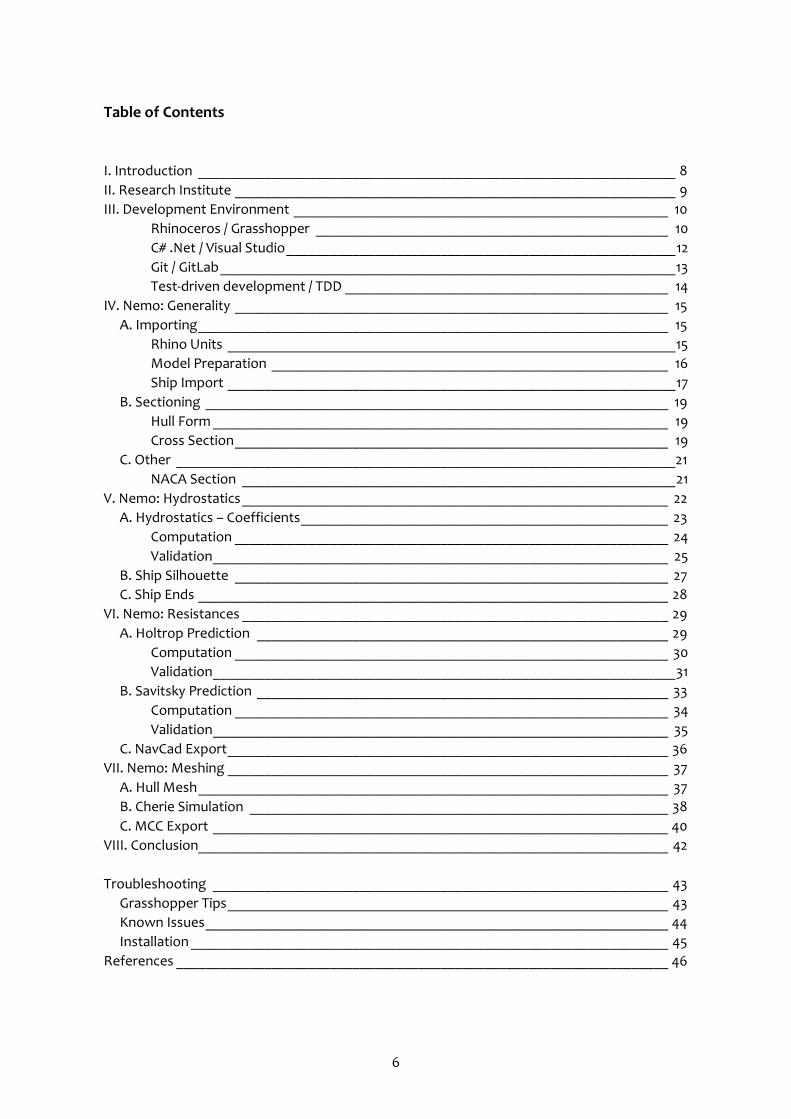
Table of Contents I. Introduction _________________________________________________________________ 8 II. Research Institute ____________________________________________________________ 9 III. Development Environment ___________________________________________________ 10

Rhinoceros / Grasshopper ________________________________________________ 10 C# .Net / Visual Studio _____________________________________________________ 12 Git / GitLab ______________________________________________________________ 13 Test-driven development / TDD ____________________________________________ 14

IV. Nemo: Generality ___________________________________________________________ 15 A. Importing ________________________________________________________________ 15

Rhino Units _____________________________________________________________ 15 Model Preparation ______________________________________________________ 16 Ship Import _____________________________________________________________ 17

B. Sectioning _______________________________________________________________ 19 Hull Form ______________________________________________________________ 19 Cross Section ___________________________________________________________ 19

C. Other ____________________________________________________________________ 21 NACA Section ___________________________________________________________ 21

V. Nemo: Hydrostatics __________________________________________________________ 22 A. Hydrostatics – Coefficients __________________________________________________ 23

Computation ___________________________________________________________ 24 Validation ______________________________________________________________ 25

B. Ship Silhouette ___________________________________________________________ 27 C. Ship Ends ________________________________________________________________ 28

VI. Nemo: Resistances __________________________________________________________ 29 A. Holtrop Prediction ________________________________________________________ 29

Computation ___________________________________________________________ 30 Validation _______________________________________________________________ 31

B. Savitsky Prediction ________________________________________________________ 33 Computation ___________________________________________________________ 34 Validation ______________________________________________________________ 35

C. NavCad Export ____________________________________________________________ 36 VII. Nemo: Meshing ____________________________________________________________ 37

A. Hull Mesh ________________________________________________________________ 37 B. Cherie Simulation _________________________________________________________ 38 C. MCC Export ______________________________________________________________ 40

VIII. Conclusion________________________________________________________________ 42 Troubleshooting ______________________________________________________________ 43

Grasshopper Tips ____________________________________________________________ 43 Known Issues _______________________________________________________________ 44 Installation _________________________________________________________________ 45

References ___________________________________________________________________ 46

7

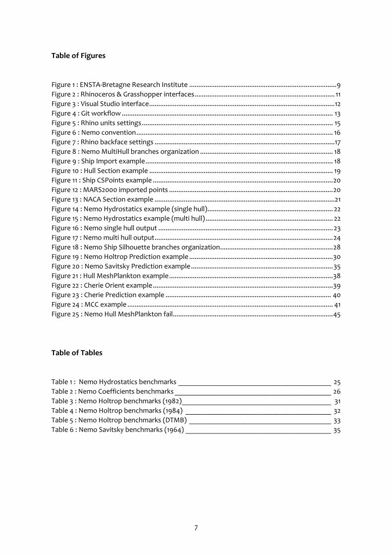
Table of Figures Figure 1 : ENSTA-Bretagne Research Institute ................................................................................. 9 Figure 2 : Rhinoceros & Grasshopper interfaces ............................................................................. 11 Figure 3 : Visual Studio interface ...................................................................................................... 12 Figure 4 : Git workflow .................................................................................................................... 13 Figure 5 : Rhino units settings ......................................................................................................... 15 Figure 6 : Nemo convention ............................................................................................................ 16 Figure 7 : Rhino backface settings ...................................................................................................17 Figure 8 : Nemo MultiHull branches organization ......................................................................... 18 Figure 9 : Ship Import example ....................................................................................................... 18 Figure 10 : Hull Section example ..................................................................................................... 19 Figure 11 : Ship CSPoints example ................................................................................................... 20 Figure 12 : MARS2000 imported points .......................................................................................... 20 Figure 13 : NACA Section example ................................................................................................... 21 Figure 14 : Nemo Hydrostatics example (single hull) ..................................................................... 22 Figure 15 : Nemo Hydrostatics example (multi hull) ...................................................................... 22 Figure 16 : Nemo single hull output ................................................................................................ 23 Figure 17 : Nemo multi hull output .................................................................................................. 24 Figure 18 : Nemo Ship Silhouette branches organization .............................................................. 28 Figure 19 : Nemo Holtrop Prediction example ............................................................................... 30 Figure 20 : Nemo Savitsky Prediction example .............................................................................. 35 Figure 21 : Hull MeshPlankton example .......................................................................................... 38 Figure 22 : Cherie Orient example ................................................................................................... 39 Figure 23 : Cherie Prediction example ........................................................................................... 40 Figure 24 : MCC example ................................................................................................................. 41 Figure 25 : Nemo Hull MeshPlankton fail ........................................................................................ 45 Table of Tables Table 1 : Nemo Hydrostatics benchmarks __________________________________________ 25 Table 2 : Nemo Coefficients benchmarks ___________________________________________ 26 Table 3 : Nemo Holtrop benchmarks (1982) _________________________________________ 31 Table 4 : Nemo Holtrop benchmarks (1984) ________________________________________ 32 Table 5 : Nemo Holtrop benchmarks (DTMB) _______________________________________ 33 Table 6 : Nemo Savitsky benchmarks (1964) ________________________________________ 35

8

I. Introduction In ship design, time saving and interoperability are two important factors for efficiency and productivity, many steps need continuous back and forth to converge the project loop. These back and forth are most of the time exchanges between individual software (modelling, stability, structure, seakeeping, resistance prediction, flow simulation, etc), and requires rigorous management and optimization of these exchanges. In such context, Rhino has a central position, either to send ship model data to external software, or to receive results from these and re-inject modifications to model. As mentioned before, the purpose is to integrate a maximum number of tools for ship design that can be performed directly inside Rhino, and otherwise to optimize the management and data exchange with external software. Another important aspect that starts showing up, is the notion of interoperability. While many industrial software wants to bring an all-in-one solution on the market, the ideology here is not to have the pretention to be better than a specialized one and not trying to replace it. As said before, Rhino is a central platform used everywhere in naval industry, and this position is extremely interesting to push forward exchanges support and try to have better seamless workflows. These researches take place in the frame of my MSc internship at Engineering School of Advanced Technologies of Brittany (ENSTA Bretagne). My supervisors are Pierre-Michel GUILCHER and Jean-Marc LAURENS, Naval and Offshore Engineering Programme Head at ENSTA Bretagne. This report is composed of several parts showing, to start, the research laboratory context, then the development working environment used. Main following parts explain Nemo functionalities and expose the passed tests. These parts are split as Nemo Generality, Hydrostatics, Resistances, and Meshing topics. Troubleshooting and References are presented in appendix. ---------- As Nemo is continuously growing up, any feedback and improvements are highly appreciated. Please feel free to contact me directly by email : nemo@mathieuvenot.com

Nemo is licensed under the Creative Commons Attribution-NonCommercial-NoDerivatives 4.0 International License (CC BY-NC-ND 4.0). You are free to share, copy and redistribute the plugin. You must give appropriate credit, provide a link to the license, and indicate if changes were made. You may not use the plugin for commercial purposes. If you remix, transform, or build upon the plugin, you may not distribute the modified plugin. You may not apply legal terms or technological measures that legally restrict others from doing anything the license permits. No warranties are given.

9

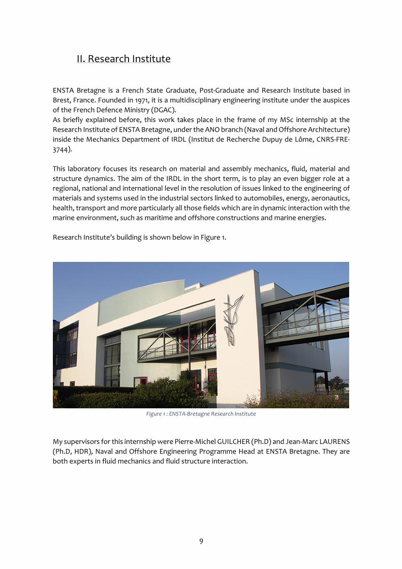
II. Research Institute ENSTA Bretagne is a French State Graduate, Post-Graduate and Research Institute based in Brest, France. Founded in 1971, it is a multidisciplinary engineering institute under the auspices of the French Defence Ministry (DGAC). As briefly explained before, this work takes place in the frame of my MSc internship at the Research Institute of ENSTA Bretagne, under the ANO branch (Naval and Offshore Architecture) inside the Mechanics Department of IRDL (Institut de Recherche Dupuy de Lôme, CNRS-FRE-3744). This laboratory focuses its research on material and assembly mechanics, fluid, material and structure dynamics. The aim of the IRDL in the short term, is to play an even bigger role at a regional, national and international level in the resolution of issues linked to the engineering of materials and systems used in the industrial sectors linked to automobiles, energy, aeronautics, health, transport and more particularly all those fields which are in dynamic interaction with the marine environment, such as maritime and offshore constructions and marine energies. Research Institute’s building is shown below in Figure 1.

Figure 1 : ENSTA-Bretagne Research Institute

My supervisors for this internship were Pierre-Michel GUILCHER (Ph.D) and Jean-Marc LAURENS (Ph.D, HDR), Naval and Offshore Engineering Programme Head at ENSTA Bretagne. They are both experts in fluid mechanics and fluid structure interaction.

10

III. Development Environment

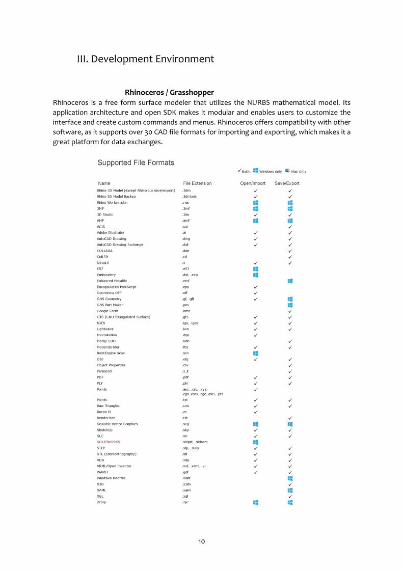
Rhinoceros / Grasshopper Rhinoceros is a free form surface modeler that utilizes the NURBS mathematical model. Its application architecture and open SDK makes it modular and enables users to customize the interface and create custom commands and menus. Rhinoceros offers compatibility with other software, as it supports over 30 CAD file formats for importing and exporting, which makes it a great platform for data exchanges.

11

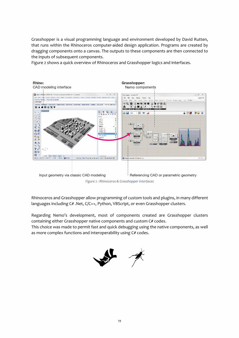
Grasshopper is a visual programming language and environment developed by David Rutten, that runs within the Rhinoceros computer-aided design application. Programs are created by dragging components onto a canvas. The outputs to these components are then connected to the inputs of subsequent components. Figure 2 shows a quick overview of Rhinoceros and Grasshopper logics and interfaces.

Figure 2 : Rhinoceros & Grasshopper interfaces

Rhinoceros and Grasshopper allow programming of custom tools and plugins, in many different languages including C# .Net, C/C++, Python, VBScript, or even Grasshopper clusters. Regarding Nemo’s development, most of components created are Grasshopper clusters containing either Grasshopper native components and custom C# codes. This choice was made to permit fast and quick debugging using the native components, as well as more complex functions and interoperability using C# codes.

12

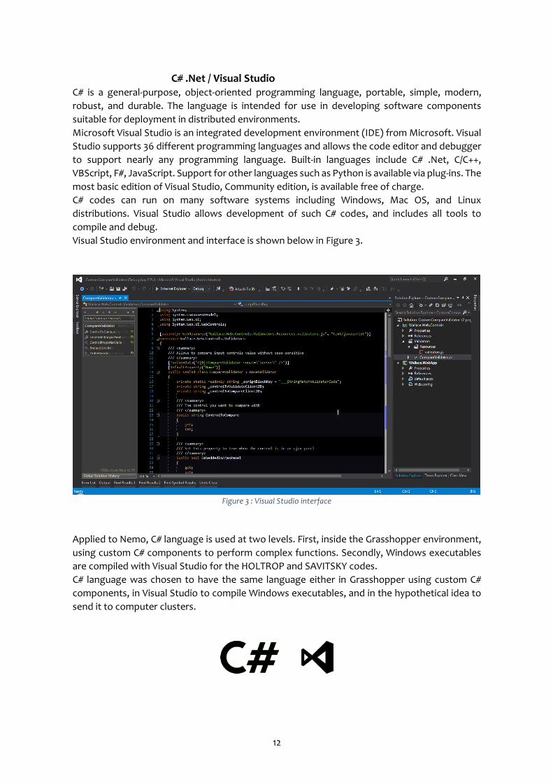
C# .Net / Visual Studio C# is a general-purpose, object-oriented programming language, portable, simple, modern, robust, and durable. The language is intended for use in developing software components suitable for deployment in distributed environments. Microsoft Visual Studio is an integrated development environment (IDE) from Microsoft. Visual Studio supports 36 different programming languages and allows the code editor and debugger to support nearly any programming language. Built-in languages include C# .Net, C/C++, VBScript, F#, JavaScript. Support for other languages such as Python is available via plug-ins. The most basic edition of Visual Studio, Community edition, is available free of charge. C# codes can run on many software systems including Windows, Mac OS, and Linux distributions. Visual Studio allows development of such C# codes, and includes all tools to compile and debug. Visual Studio environment and interface is shown below in Figure 3.

Figure 3 : Visual Studio interface

Applied to Nemo, C# language is used at two levels. First, inside the Grasshopper environment, using custom C# components to perform complex functions. Secondly, Windows executables are compiled with Visual Studio for the HOLTROP and SAVITSKY codes. C# language was chosen to have the same language either in Grasshopper using custom C# components, in Visual Studio to compile Windows executables, and in the hypothetical idea to send it to computer clusters.

13

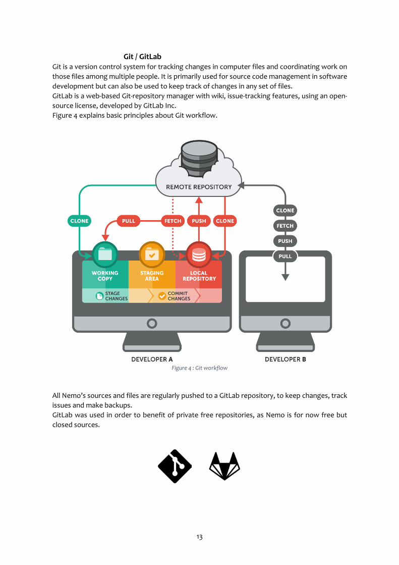
Git / GitLab Git is a version control system for tracking changes in computer files and coordinating work on those files among multiple people. It is primarily used for source code management in software development but can also be used to keep track of changes in any set of files. GitLab is a web-based Git-repository manager with wiki, issue-tracking features, using an open-source license, developed by GitLab Inc. Figure 4 explains basic principles about Git workflow.

Figure 4 : Git workflow

All Nemo’s sources and files are regularly pushed to a GitLab repository, to keep changes, track issues and make backups. GitLab was used in order to benefit of private free repositories, as Nemo is for now free but closed sources.

14

Test-driven development / TDD Test-driven development (TDD) is a software development process that relies on the repetition of a very short development cycle: requirements are turned into very specific test cases, then the software is improved to pass the new tests, only. Considering Nemo’s development, a series of benchmarks were performed comparing Nemo’s values to analytic solutions and leading software in the field (MAAT HYDRO, NAVCAD, or ORCA3D), before validating the computations performed and engaging the next development stage.

15

IV. Nemo: Generality This first part exposes important steps to proceed when starting using Nemo, in particular the model preparation operated by the user before importing his own designs. Following subsections explain additional tools provided, like drawing utilities and NACA section generator. Regarding the validation process, mainly used in the Hydrostatics and Resistances computations, value comparisons are tested over several sources. A general example case is performed using the US Navy Combatant DTMB 5415 INSEAN model, and given numerical examples in HOLTROP and SAVITSKY papers are checked. Please note important remark about computational speed. As Nemo is working on NURBS geometry directly, time consuming is important, please keep that in mind. A quick tip to explain how to enabled / disabled components is exposed in Troubleshooting section.

A. Importing

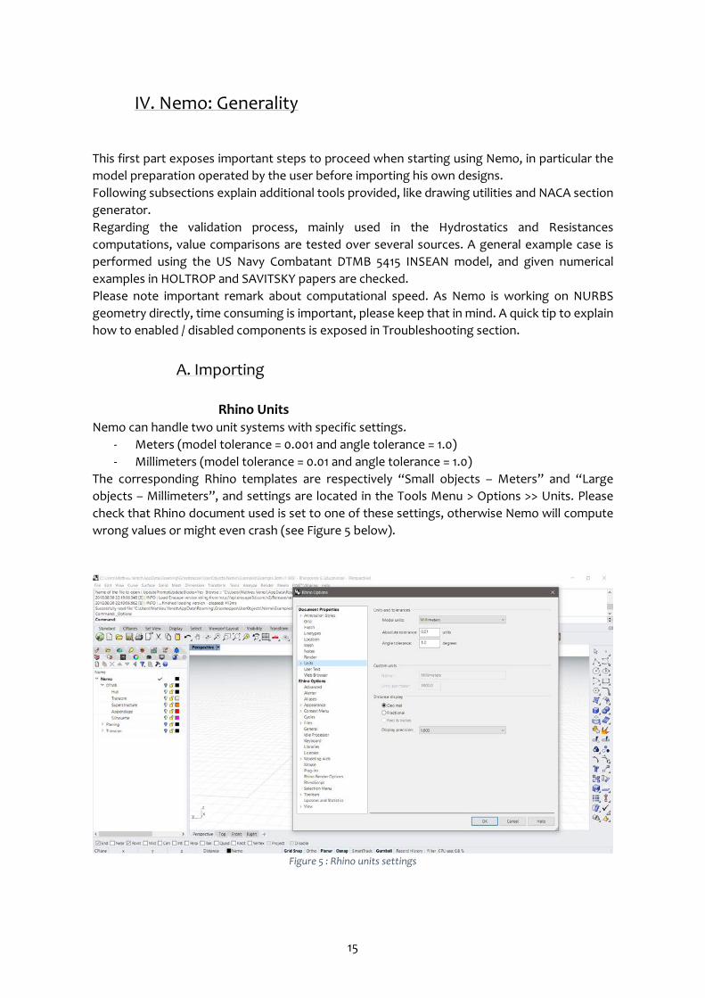
Rhino Units Nemo can handle two unit systems with specific settings.

- Meters (model tolerance = 0.001 and angle tolerance = 1.0) - Millimeters (model tolerance = 0.01 and angle tolerance = 1.0)

The corresponding Rhino templates are respectively “Small objects – Meters” and “Large objects – Millimeters”, and settings are located in the Tools Menu > Options >> Units. Please check that Rhino document used is set to one of these settings, otherwise Nemo will compute wrong values or might even crash (see Figure 5 below).

Figure 5 : Rhino units settings

16

Another important thing is about the values computed and used by Nemo, especially for component’s inputs and outputs. If Nemo need or compute a value with a specific unit, it will be explicitly shown when hovering the input or output of components with mouse cursor. Otherwise, if no unit is explicitly shown, it need or use the Rhino document. Same logic is used for geometry needs. It will be explicitly asking for complete hull (starboard + portside), half hull (portside only), and either joined as 1 polysurface or not.

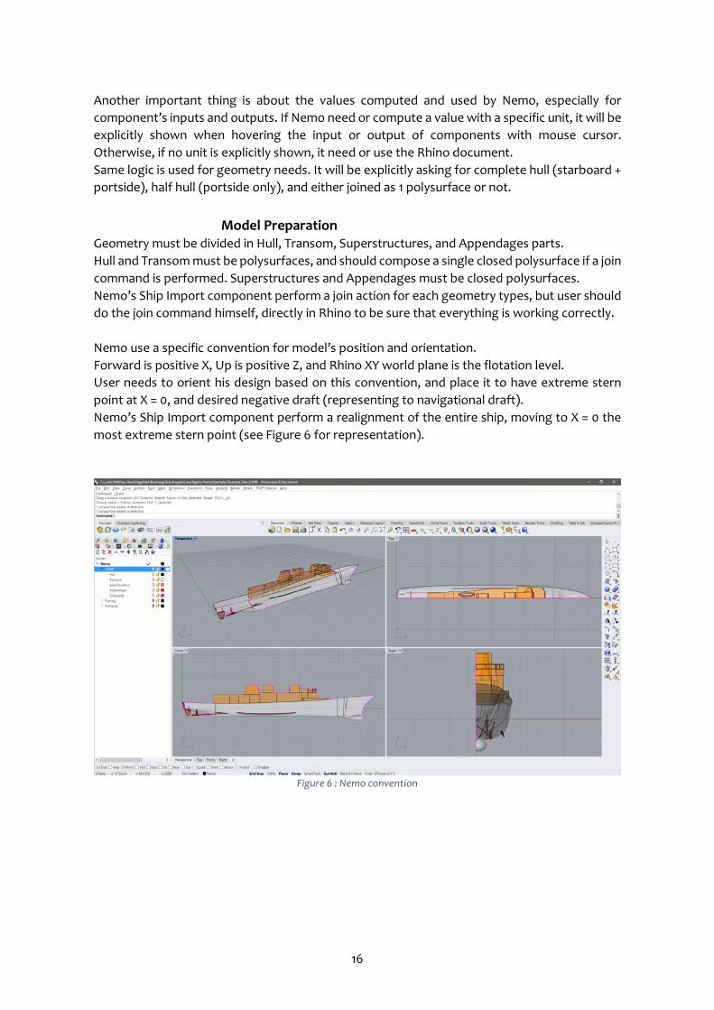
Model Preparation Geometry must be divided in Hull, Transom, Superstructures, and Appendages parts. Hull and Transom must be polysurfaces, and should compose a single closed polysurface if a join command is performed. Superstructures and Appendages must be closed polysurfaces. Nemo’s Ship Import component perform a join action for each geometry types, but user should do the join command himself, directly in Rhino to be sure that everything is working correctly. Nemo use a specific convention for model’s position and orientation. Forward is positive X, Up is positive Z, and Rhino XY world plane is the flotation level. User needs to orient his design based on this convention, and place it to have extreme stern point at X = 0, and desired negative draft (representing to navigational draft). Nemo’s Ship Import component perform a realignment of the entire ship, moving to X = 0 the most extreme stern point (see Figure 6 for representation).

Figure 6 : Nemo convention

17

Geometry’s normals need to be correctly oriented, pointing out, looking to the exterior of the hull or geometries. Nemo’s Ship Import component can display imported geometry and normals preview as shown in Figure 9, Rhino can also draw backfaces with another colour (Tools Menu > Options >> View >> Display Modes >> “Name” >>> Backface settings >>>> Single color for all backfaces, see Figure 7).

Figure 7 : Rhino backface settings

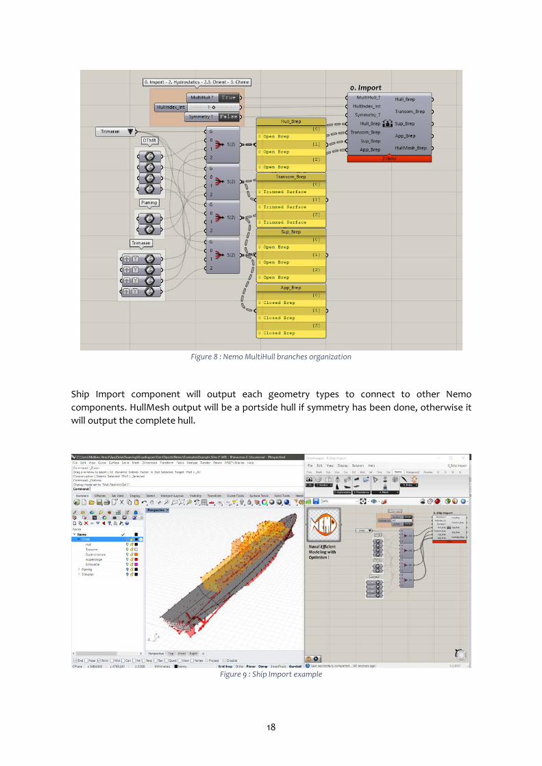
Ship Import Import ship geometry from Rhino, perform XZ symmetry if needed, and deal with multi or single hull configurations. Hull, Transom, Sup and App inputs can be set connecting Grasshopper’s Brep components (Params tab > Geometry) Right-Click on it to select Set Multiple Breps option, or use Grasshopper’s Geometry Pipeline components (Params tab > Geometry) to pick geometry directly from Rhino layers. Symmetry can be performed on XZ plane connecting a Grasshopper’s Boolean Toggle component (Params tab > Input), set it to True of symmetry is needed. MultiHull and HullIndex settings are used to deal with multiple hull import and quickly isolate a single hull. MultiHull input can be set connecting a Grasshopper’s Boolean Toggle component (Params tab > Input), and HullIndex with a Grasshopper’s Slider component (Params tab > Input). If MultiHull is set to True, Ship Import component will return all geometry used in input. If it is set to False, use the HullIndex to choose which hull to isolate. Hull isolation using HullIndex needs to have a correctly organized inputs, geometry sorted by branches. Hull(0) should match with Transom(0) + Sup(0) + App(0), then Hull(1) with Transom(1) + Sup(1) + App(1), etc. See Trimaran model in examples files provided with Nemo, Figure 8.

18

Figure 8 : Nemo MultiHull branches organization

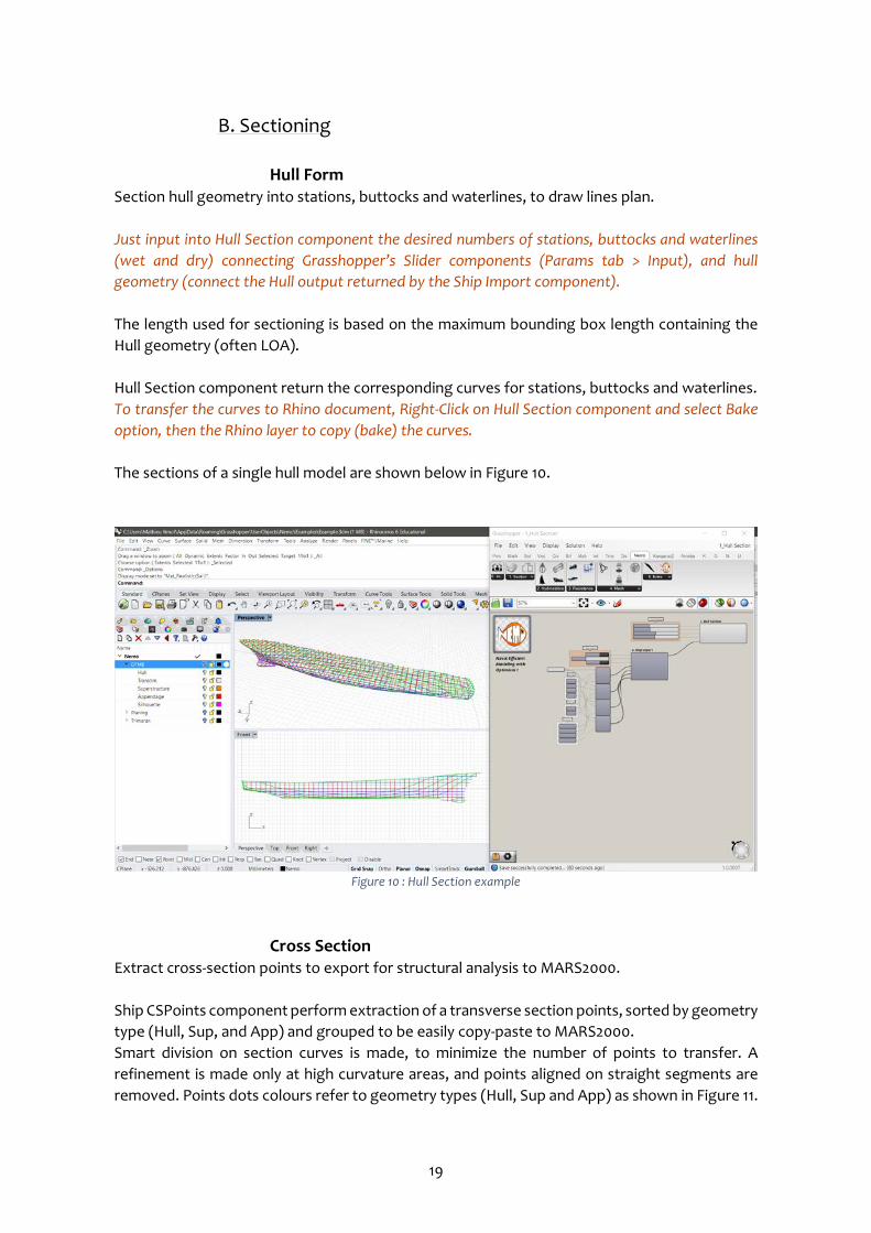
Ship Import component will output each geometry types to connect to other Nemo components. HullMesh output will be a portside hull if symmetry has been done, otherwise it will output the complete hull.

Figure 9 : Ship Import example

19

B. Sectioning

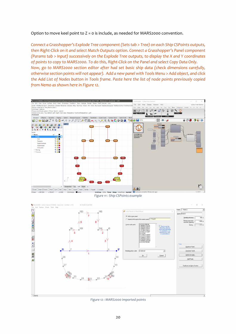
Hull Form Section hull geometry into stations, buttocks and waterlines, to draw lines plan. Just input into Hull Section component the desired numbers of stations, buttocks and waterlines (wet and dry) connecting Grasshopper’s Slider components (Params tab > Input), and hull geometry (connect the Hull output returned by the Ship Import component). The length used for sectioning is based on the maximum bounding box length containing the Hull geometry (often LOA). Hull Section component return the corresponding curves for stations, buttocks and waterlines. To transfer the curves to Rhino document, Right-Click on Hull Section component and select Bake option, then the Rhino layer to copy (bake) the curves. The sections of a single hull model are shown below in Figure 10.

Figure 10 : Hull Section example

Cross Section Extract cross-section points to export for structural analysis to MARS2000. Ship CSPoints component perform extraction of a transverse section points, sorted by geometry type (Hull, Sup, and App) and grouped to be easily copy-paste to MARS2000. Smart division on section curves is made, to minimize the number of points to transfer. A refinement is made only at high curvature areas, and points aligned on straight segments are removed. Points dots colours refer to geometry types (Hull, Sup and App) as shown in Figure 11.

20

Option to move keel point to Z = 0 is include, as needed for MARS2000 convention. Connect a Grasshopper’s Explode Tree component (Sets tab > Tree) on each Ship CSPoints outputs, then Right-Click on it and select Match Outputs option. Connect a Grasshopper’s Panel component (Params tab > Input) successively on the Explode Tree outputs, to display the X and Y coordinates of points to copy to MARS2000. To do this, Right-Click on the Panel and select Copy Data Only. Now, go to MARS2000 section editor after had set basic ship data (check dimensions carefully, otherwise section points will not appear). Add a new panel with Tools Menu > Add object, and click the Add List of Nodes button in Tools frame. Paste here the list of node points previously copied from Nemo as shown here in Figure 12.

Figure 11 : Ship CSPoints example

Figure 12 : MARS2000 imported points

21

C. Other

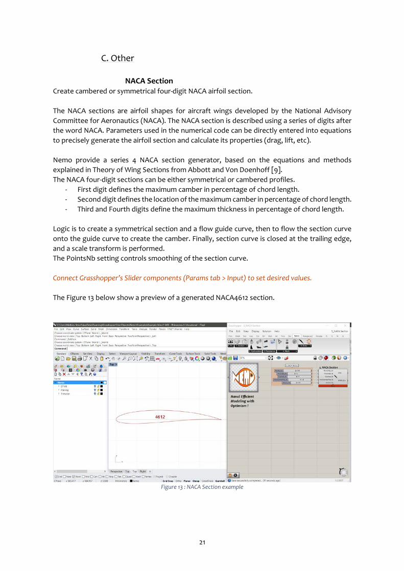
NACA Section Create cambered or symmetrical four-digit NACA airfoil section. The NACA sections are airfoil shapes for aircraft wings developed by the National Advisory Committee for Aeronautics (NACA). The NACA section is described using a series of digits after the word NACA. Parameters used in the numerical code can be directly entered into equations to precisely generate the airfoil section and calculate its properties (drag, lift, etc). Nemo provide a series 4 NACA section generator, based on the equations and methods explained in Theory of Wing Sections from Abbott and Von Doenhoff [9]. The NACA four-digit sections can be either symmetrical or cambered profiles.

- First digit defines the maximum camber in percentage of chord length. - Second digit defines the location of the maximum camber in percentage of chord length. - Third and Fourth digits define the maximum thickness in percentage of chord length.

Logic is to create a symmetrical section and a flow guide curve, then to flow the section curve onto the guide curve to create the camber. Finally, section curve is closed at the trailing edge, and a scale transform is performed. The PointsNb setting controls smoothing of the section curve. Connect Grasshopper’s Slider components (Params tab > Input) to set desired values. The Figure 13 below show a preview of a generated NACA4612 section.

Figure 13 : NACA Section example

22

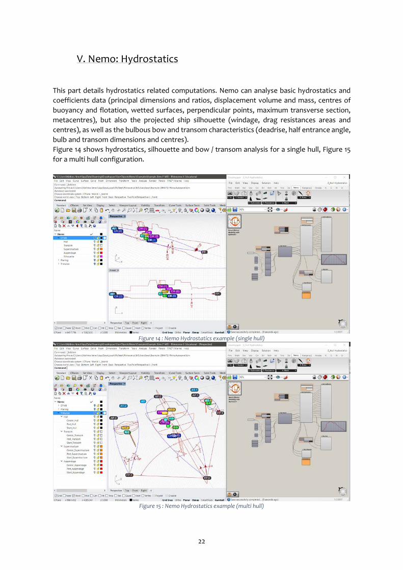
V. Nemo: Hydrostatics This part details hydrostatics related computations. Nemo can analyse basic hydrostatics and coefficients data (principal dimensions and ratios, displacement volume and mass, centres of buoyancy and flotation, wetted surfaces, perpendicular points, maximum transverse section, metacentres), but also the projected ship silhouette (windage, drag resistances areas and centres), as well as the bulbous bow and transom characteristics (deadrise, half entrance angle, bulb and transom dimensions and centres). Figure 14 shows hydrostatics, silhouette and bow / transom analysis for a single hull, Figure 15 for a multi hull configuration.

Figure 14 : Nemo Hydrostatics example (single hull)

Figure 15 : Nemo Hydrostatics example (multi hull)

23

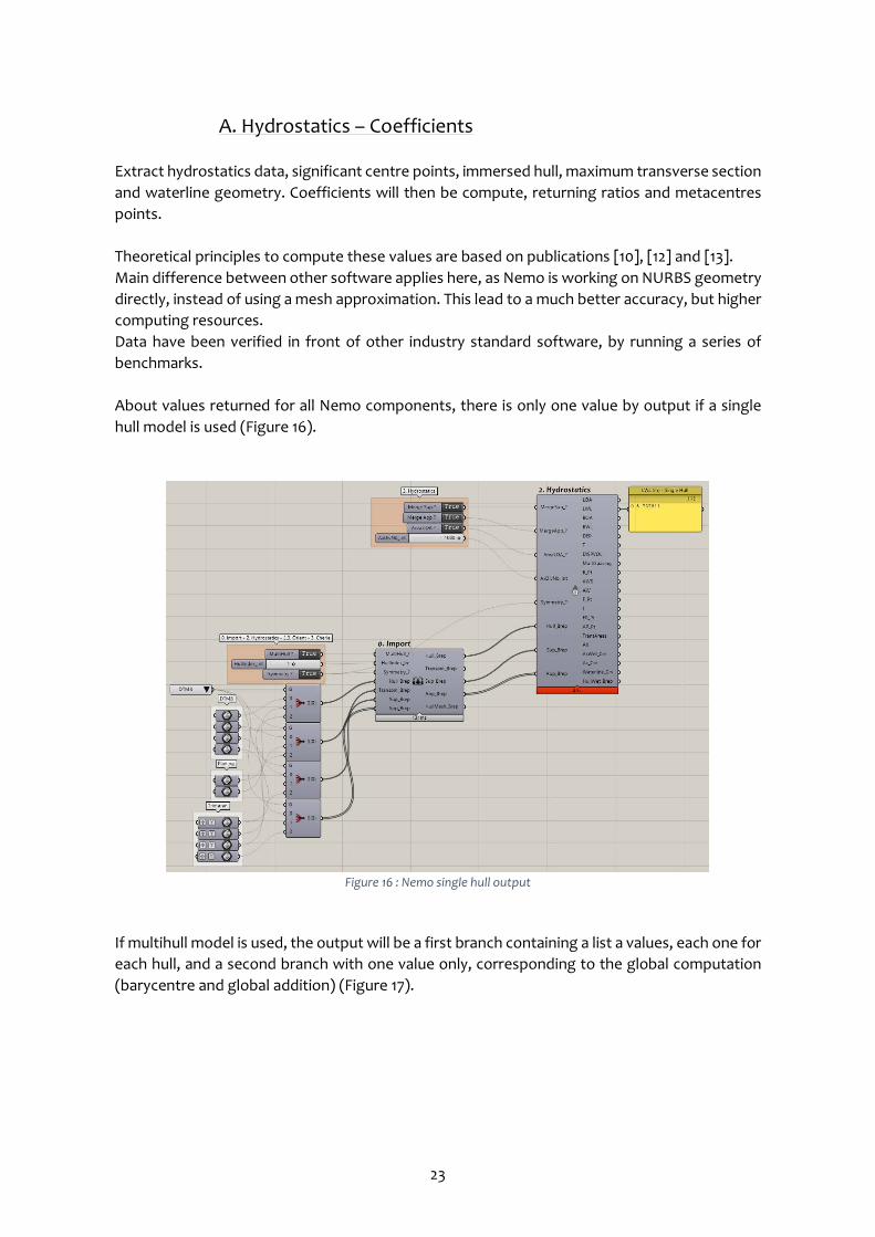
A. Hydrostatics – Coefficients Extract hydrostatics data, significant centre points, immersed hull, maximum transverse section and waterline geometry. Coefficients will then be compute, returning ratios and metacentres points. Theoretical principles to compute these values are based on publications [10], [12] and [13]. Main difference between other software applies here, as Nemo is working on NURBS geometry directly, instead of using a mesh approximation. This lead to a much better accuracy, but higher computing resources. Data have been verified in front of other industry standard software, by running a series of benchmarks. About values returned for all Nemo components, there is only one value by output if a single hull model is used (Figure 16).

Figure 16 : Nemo single hull output

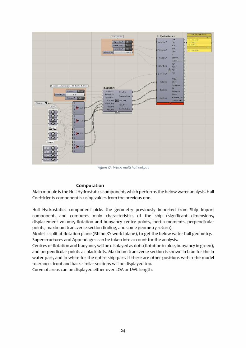
If multihull model is used, the output will be a first branch containing a list a values, each one for each hull, and a second branch with one value only, corresponding to the global computation (barycentre and global addition) (Figure 17).

24

Figure 17 : Nemo multi hull output

Computation Main module is the Hull Hydrostatics component, which performs the below water analysis. Hull Coefficients component is using values from the previous one. Hull Hydrostatics component picks the geometry previously imported from Ship Import component, and computes main characteristics of the ship (significant dimensions, displacement volume, flotation and buoyancy centre points, inertia moments, perpendicular points, maximum transverse section finding, and some geometry return). Model is split at flotation plane (Rhino XY world plane), to get the below water hull geometry. Superstructures and Appendages can be taken into account for the analysis. Centres of flotation and buoyancy will be displayed as dots (flotation in blue, buoyancy in green), and perpendicular points as black dots. Maximum transverse section is shown in blue for the in water part, and in white for the entire ship part. If there are other positions within the model tolerance, front and back similar sections will be displayed too. Curve of areas can be displayed either over LOA or LWL length.

25

Inputs are Grasshopper’s Toggle components (Params tab > Input) to define if Superstructure and Appendages will be used (True) or not (False) for hydrostatics analysis, to define if curve of areas will be plotted over LOA (True) or LWL (False), and if symmetry has been performed (True) or not (False). AxDivNb use a Grasshopper’s Slider component (Params > Tab) to define the number of transverse sections computed to find the maximum one. Start with a low number, because intersections are made over NURBS geometry again, and can take times to compute. Connect geometry inputs directly to the corresponding outputs of Ship Import component. Hull Coefficients use data extracted by the Hull Hydrostatics component to compute ship coefficients and ratios, as well as the displacement mass and metacentres. Metacentres are displayed as blue dots for longitudinal ones and as yellow dots for transverse ones. Simply connect inputs the corresponding outputs of Hull Hydrostatics component.

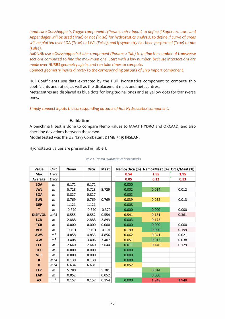
Validation A benchmark test is done to compare Nemo values to MAAT HYDRO and ORCA3D, and also checking deviations between these two. Model tested was the US Navy Combatant DTMB 5415 INSEAN. Hydrostatics values are presented in Table 1.

Table 1 : Nemo Hydrostatics benchmarks

Value Unit Nemo Orca Maat Nemo/Orca (%) Nemo/Maat (%) Orca/Maat (%)Max Error 0.54 1.95 1.95

Average Error 0.05 0.12 0.13LOA m 6.172 6.172 0.000LWL m 5.728 5.728 5.729 0.002 0.014 0.012BOA m 0.827 0.827 0.002BWL m 0.769 0.769 0.769 0.039 0.052 0.013DEP m 1.121 1.121 0.008

T m -0.370 -0.370 -0.370 0.000 0.000 0.000DISPVOL m^3 0.555 0.552 0.554 0.541 0.181 0.361

LCB m 2.888 2.888 2.893 0.003 0.173TCB m 0.000 0.000 0.000 0.000 0.000 0.000VCB m -0.101 -0.101 -0.101 0.199 0.000 0.199AWS m² 4.858 4.855 4.856 0.062 0.041 0.021AW m² 3.408 3.406 3.407 0.051 0.013 0.038LCF m 2.640 2.640 2.644 0.011 0.140 0.129TCF m 0.000 0.000 0.000VCF m 0.000 0.000 0.000

It m^4 0.130 0.130 0.000Il m^4 6.634 6.631 0.052

LFP m 5.780 5.781 0.014LAP m 0.052 0.052 0.000AX m² 0.157 0.157 0.154 0.000 1.948 1.948

26

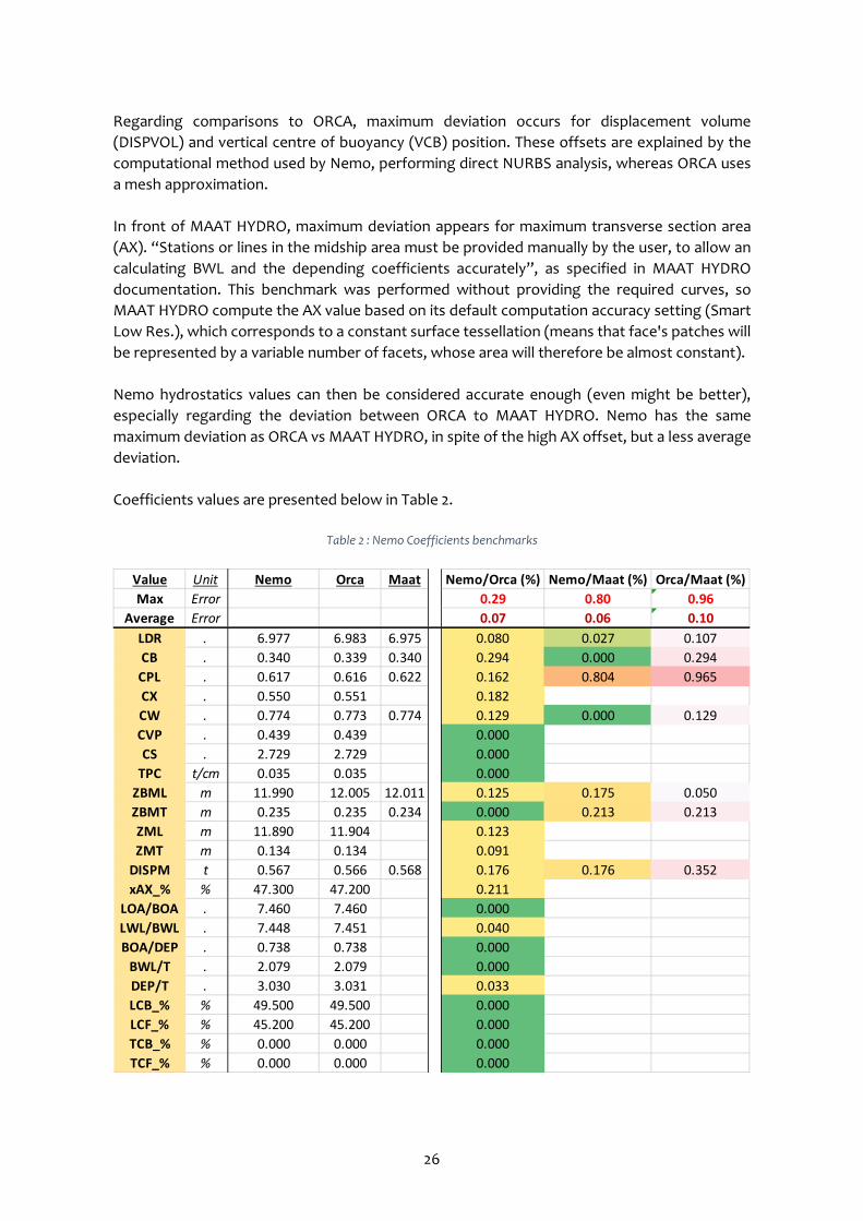
Regarding comparisons to ORCA, maximum deviation occurs for displacement volume (DISPVOL) and vertical centre of buoyancy (VCB) position. These offsets are explained by the computational method used by Nemo, performing direct NURBS analysis, whereas ORCA uses a mesh approximation. In front of MAAT HYDRO, maximum deviation appears for maximum transverse section area (AX). “Stations or lines in the midship area must be provided manually by the user, to allow an calculating BWL and the depending coefficients accurately”, as specified in MAAT HYDRO documentation. This benchmark was performed without providing the required curves, so MAAT HYDRO compute the AX value based on its default computation accuracy setting (Smart Low Res.), which corresponds to a constant surface tessellation (means that face's patches will be represented by a variable number of facets, whose area will therefore be almost constant). Nemo hydrostatics values can then be considered accurate enough (even might be better), especially regarding the deviation between ORCA to MAAT HYDRO. Nemo has the same maximum deviation as ORCA vs MAAT HYDRO, in spite of the high AX offset, but a less average deviation. Coefficients values are presented below in Table 2.

Table 2 : Nemo Coefficients benchmarks

Value Unit Nemo Orca Maat Nemo/Orca (%) Nemo/Maat (%) Orca/Maat (%)Max Error 0.29 0.80 0.96

Average Error 0.07 0.06 0.10LDR . 6.977 6.983 6.975 0.080 0.027 0.107CB . 0.340 0.339 0.340 0.294 0.000 0.294CPL . 0.617 0.616 0.622 0.162 0.804 0.965CX . 0.550 0.551 0.182CW . 0.774 0.773 0.774 0.129 0.000 0.129CVP . 0.439 0.439 0.000CS . 2.729 2.729 0.000

TPC t/cm 0.035 0.035 0.000ZBML m 11.990 12.005 12.011 0.125 0.175 0.050ZBMT m 0.235 0.235 0.234 0.000 0.213 0.213ZML m 11.890 11.904 0.123ZMT m 0.134 0.134 0.091

DISPM t 0.567 0.566 0.568 0.176 0.176 0.352xAX_% % 47.300 47.200 0.211

LOA/BOA . 7.460 7.460 0.000LWL/BWL . 7.448 7.451 0.040BOA/DEP . 0.738 0.738 0.000

BWL/T . 2.079 2.079 0.000DEP/T . 3.030 3.031 0.033LCB_% % 49.500 49.500 0.000LCF_% % 45.200 45.200 0.000TCB_% % 0.000 0.000 0.000TCF_% % 0.000 0.000 0.000

27

Same conclusion to say here, because data are based on the previous values from hydrostatics computation, maximum deviation appears to be on the prismatic coefficient (CPL) which is based on AX value.

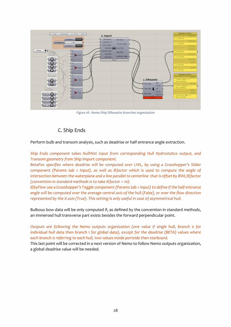
B. Ship Silhouette Extract windage and water resistance analysis, compute areas and centre points, as well as giving the silhouette profile curve. Previews are shown in the Figure 14 and Figure 15, in addition to the other hydrostatics and bow / transom computations also displayed in these pictures. Be careful, Ship Silhouette component can be very slow, depending of the complexity of geometry used. Hull, Superstructures and Appendages profiles are projected onto the XZ (longitudinal) and YZ (transverse) planes, before computing the analysis. This component returns a specific branches organization, ordered by geometry type (see Figure 18 below). An empty branch means that the geometry type corresponding to this branch has no effect on wind or water resistance. CW (purple dots) and CR (blue dots) points are sorted in branches as follow: {0;0} = Hull part {0;1} = Superstructures part {0;2} = Appendages part {1;0} = Global barycentre WA and RA areas are sorted in the same way, but return either the longitudinal and transverse projection areas: {0;0;0} = Hull longitudinal area {0;0;1} = Superstructures longitudinal area {0;0;2} = Appendages longitudinal area {0;1;0} = Hull transverse area {0;1;1} = Superstructure transverse area {0;1;2} = Appendages transverse area {1;0} = Global longitudinal area {1;1} = Global transverse area Simply connect geometry inputs directly to the corresponding outputs of Ship Import component. The silhouette profile curve can be used when exporting to MAAT HYDRO, and values computed are taken into account further by the NavCad Export component.

28

Figure 18 : Nemo Ship Silhouette branches organization

C. Ship Ends Perform bulb and transom analysis, such as deadrise or half entrance angle extraction. Ship Ends component takes HullWet input from corresponding Hull Hydrostatics output, and Transom geometry from Ship Import component. BetaPos specifies where deadrise will be computed over LWL, by using a Grasshopper’s Slider component (Params tab > Input), as well as IEfactor which is used to compute the angle of intersection between the waterplane and a line parallel to centerline that is offset by BWL/IEfactor (convention in standard methods is to take IEfactor = 10). IEbyFlow use a Grasshopper’s Toggle component (Params tab > Input) to define if the half entrance angle will be computed over the average central axis of the hull (False), or over the flow direction represented by the X axis (True). This setting is only useful in case of asymmetrical hull. Bulbous bow data will be only computed if, as defined by the convention in standard methods, an immersed hull transverse part exists besides the forward perpendicular point. Outputs are following the Nemo outputs organization (one value if single hull, branch 0 for individual hull data then branch 1 for global data), except for the deadrise (BETA) values where each branch is referring to each hull, two values inside portside then starboard. This last point will be corrected in a next version of Nemo to follow Nemo outputs organization, a global deadrise value will be needed.

29

VI. Nemo: Resistances In this section, resistance computations are detailed. Nemo provides two embed resistance prediction codes based on HOLTROP and SAVITSKY methods (statistical regressions and empirical formulas). A NAVCAD export tool from hydrostatics data is also provided. HOLTROP code includes the 1984 method, referring to the publications [1] [2] [3] [4]. Due to lack of time and not enough validation data, paper [5] of 1988 method has not been added. SAVITSKY code includes the 1964 method, referring to the publication [6]. As well, due to lack of time, paper [7] of 1976 method will be added in a next upgrade of Nemo. NAVCAD export is based on the .hcnc file format of NAVCAD projects, in use since 2013 version. A quick remark about HOLTROP and SAVITSKY executables is that both programs are located inside the Nemo folder from Grasshopper’s UserObjects location. Input and output files will be directly written in the corresponding resistance folder (HOLTROP or SAVITSKY folder). Other theoretical principles regarding resistance and hydrodynamics prediction were grabbed from the references [11], [14] and [15].

A. Holtrop Prediction Holtrop is a method based on statistical regression of model tests and results from ship trials. The method is used to estimate the resistance of displacement ships. The database covers a wide range of ships, and the method may be used to assess qualitatively the resistance of a ship design. A quick summary of the different versions of Holtrop method is recapitulated right here. - First paper from 1977 [1] takes into account only viscous resistance, wave resistance and correlation allowance. - In 1978’s paper [2], main modifications are made to include influence of a bulbous bow. - Next version in 1982 [3] adds numerous changes to take into account transom stern characteristics. Some modifications are made to the form factor and wave equations to deal with extreme shapes (depending of ship ratios characteristics). - Nemo’s implemented Holtrop version is from 1984’s paper [4], this one is the most commonly used version, and uses specific wave resistance equations depending of the Froude number. Form factor equation has also been quite corrected to integrate greater ship ratios. - Paper from 1988 [5] exposes important modifications like adding a speed dependent form factor equation, or added resistances from incoming waves and wind. Unfortunately, this method is deliberately not used in Nemo, because of few model tests and ship trials realized (enounced by the author himself). Future updates of Nemo could however receive the 1988 version and its corrections. Another word related to Nemo’s case. Appendage resistance is not considered, because preliminary design phases often doesn’t include it.

30

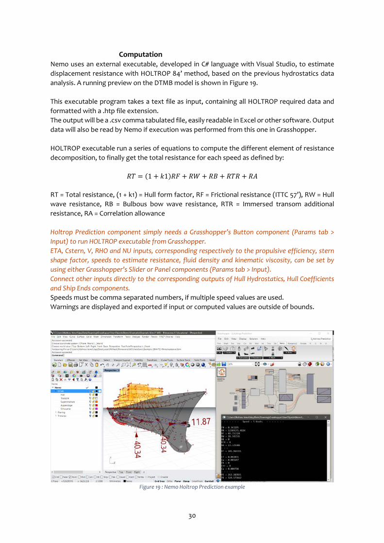
Computation Nemo uses an external executable, developed in C# language with Visual Studio, to estimate displacement resistance with HOLTROP 84’ method, based on the previous hydrostatics data analysis. A running preview on the DTMB model is shown in Figure 19. This executable program takes a text file as input, containing all HOLTROP required data and formatted with a .htp file extension. The output will be a .csv comma tabulated file, easily readable in Excel or other software. Output data will also be read by Nemo if execution was performed from this one in Grasshopper. HOLTROP executable run a series of equations to compute the different element of resistance decomposition, to finally get the total resistance for each speed as defined by:

𝑅𝑅𝑅𝑅 = (1 + 𝑘𝑘1)𝑅𝑅𝑅𝑅 + 𝑅𝑅𝑅𝑅 + 𝑅𝑅𝑅𝑅 + 𝑅𝑅𝑅𝑅𝑅𝑅 + 𝑅𝑅𝑅𝑅 RT = Total resistance, (1 + k1) = Hull form factor, RF = Frictional resistance (ITTC 57’), RW = Hull wave resistance, RB = Bulbous bow wave resistance, RTR = Immersed transom additional resistance, RA = Correlation allowance Holtrop Prediction component simply needs a Grasshopper’s Button component (Params tab > Input) to run HOLTROP executable from Grasshopper. ETA, Cstern, V, RHO and NU inputs, corresponding respectively to the propulsive efficiency, stern shape factor, speeds to estimate resistance, fluid density and kinematic viscosity, can be set by using either Grasshopper’s Slider or Panel components (Params tab > Input). Connect other inputs directly to the corresponding outputs of Hull Hydrostatics, Hull Coefficients and Ship Ends components. Speeds must be comma separated numbers, if multiple speed values are used. Warnings are displayed and exported if input or computed values are outside of bounds.

Figure 19 : Nemo Holtrop Prediction example

31

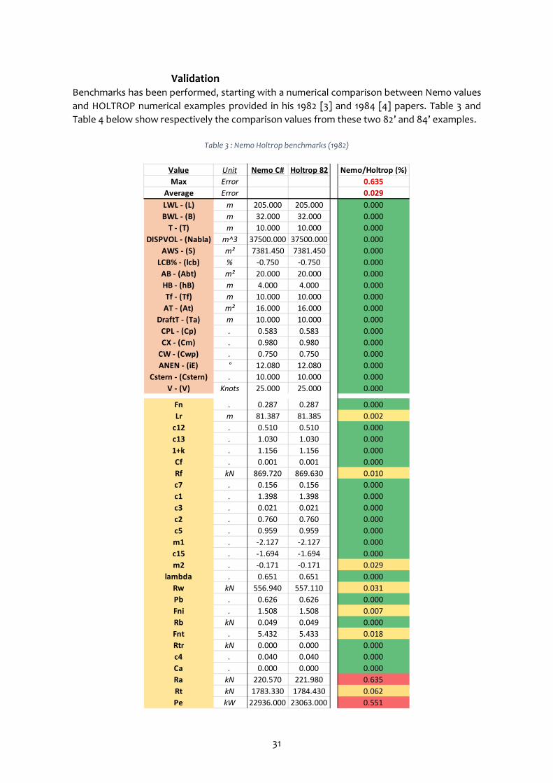
Validation Benchmarks has been performed, starting with a numerical comparison between Nemo values and HOLTROP numerical examples provided in his 1982 [3] and 1984 [4] papers. Table 3 and Table 4 below show respectively the comparison values from these two 82’ and 84’ examples.

Table 3 : Nemo Holtrop benchmarks (1982)

Value Unit Nemo C# Holtrop 82 Nemo/Holtrop (%)Max Error 0.635

Average Error 0.029LWL - (L) m 205.000 205.000 0.000BWL - (B) m 32.000 32.000 0.000

T - (T) m 10.000 10.000 0.000DISPVOL - (Nabla) m^3 37500.000 37500.000 0.000

AWS - (S) m² 7381.450 7381.450 0.000LCB% - (lcb) % -0.750 -0.750 0.000AB - (Abt) m² 20.000 20.000 0.000HB - (hB) m 4.000 4.000 0.000Tf - (Tf) m 10.000 10.000 0.000AT - (At) m² 16.000 16.000 0.000

DraftT - (Ta) m 10.000 10.000 0.000CPL - (Cp) . 0.583 0.583 0.000CX - (Cm) . 0.980 0.980 0.000

CW - (Cwp) . 0.750 0.750 0.000ANEN - (iE) ° 12.080 12.080 0.000

Cstern - (Cstern) . 10.000 10.000 0.000V - (V) Knots 25.000 25.000 0.000

Fn . 0.287 0.287 0.000Lr m 81.387 81.385 0.002

c12 . 0.510 0.510 0.000c13 . 1.030 1.030 0.0001+k . 1.156 1.156 0.000Cf . 0.001 0.001 0.000Rf kN 869.720 869.630 0.010c7 . 0.156 0.156 0.000c1 . 1.398 1.398 0.000c3 . 0.021 0.021 0.000c2 . 0.760 0.760 0.000c5 . 0.959 0.959 0.000m1 . -2.127 -2.127 0.000c15 . -1.694 -1.694 0.000m2 . -0.171 -0.171 0.029

lambda . 0.651 0.651 0.000Rw kN 556.940 557.110 0.031Pb . 0.626 0.626 0.000Fni . 1.508 1.508 0.007Rb kN 0.049 0.049 0.000Fnt . 5.432 5.433 0.018Rtr kN 0.000 0.000 0.000c4 . 0.040 0.040 0.000Ca . 0.000 0.000 0.000Ra kN 220.570 221.980 0.635Rt kN 1783.330 1784.430 0.062Pe kW 22936.000 23063.000 0.551

32

Table 4 : Nemo Holtrop benchmarks (1984)

As seen in these two tables, maximum deviation is about 0.635 % for 1982 version and 0.468 % for 1984 version. It is assumed that deviation is minimal and entirely acceptable. A second benchmark has been performed, this time by testing the HOLTROP computation over a real ship 3D model, and comparing values to NAVCAD and ORCA3D. Checking deviations between these two has also been done. Model tested was again the US Navy Combatant DTMB 5415 INSEAN. Table 5 presents this benchmark’s values.

Value Unit Nemo C# Holtrop 84 Nemo/Holtrop (%)Max Error 0.468

Average Error 0.015LWL - (L) m 50.000 50.000 0.000BWL - (B) m 12.000 12.000 0.000

T - (T) m 3.200 3.200 0.000DISPVOL - (Nabla) m^3 900.000 900.000 0.000

AWS - (S) m² 584.900 584.900 0.000LCB% - (lcb) % -4.500 -4.500 0.000AB - (Abt) m² 0.000 0.000 0.000HB - (hB) m 0.000 0.000 0.000Tf - (Tf) m 3.100 3.100 0.000AT - (At) m² 10.000 10.000 0.000

DraftT - (Ta) m 3.300 3.300 0.000CPL - (Cp) . 0.601 0.601 0.000CB - (Cb) . 0.469 0.469 0.000CX - (Cm) . 0.780 0.780 0.000

CW - (Cwp) . 0.800 0.800 0.000ANEN - (iE) ° 25.000 25.000 0.000

Cstern - (Cstern) . 0.000 0.000 0.000V - (V) Knots 25.000 25.000 0.000

Ca . 0.001 0.001 0.000lambda . 0.744 0.744 0.000Rw - kN kN 475.000 475.000 0.000Rtr - kN kN 25.000 25.000 0.000R - kN kN 638.000 641.000 0.468

33

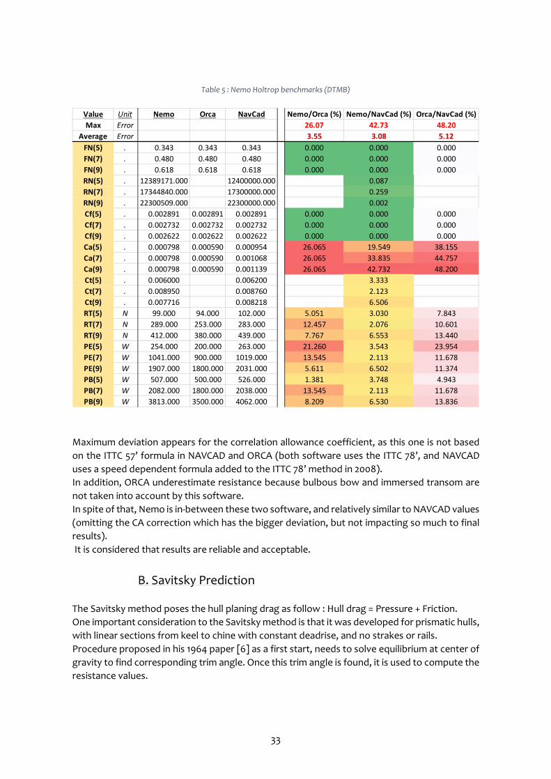
Table 5 : Nemo Holtrop benchmarks (DTMB)

Maximum deviation appears for the correlation allowance coefficient, as this one is not based on the ITTC 57’ formula in NAVCAD and ORCA (both software uses the ITTC 78’, and NAVCAD uses a speed dependent formula added to the ITTC 78’ method in 2008). In addition, ORCA underestimate resistance because bulbous bow and immersed transom are not taken into account by this software. In spite of that, Nemo is in-between these two software, and relatively similar to NAVCAD values (omitting the CA correction which has the bigger deviation, but not impacting so much to final results). It is considered that results are reliable and acceptable.

B. Savitsky Prediction The Savitsky method poses the hull planing drag as follow : Hull drag = Pressure + Friction. One important consideration to the Savitsky method is that it was developed for prismatic hulls, with linear sections from keel to chine with constant deadrise, and no strakes or rails. Procedure proposed in his 1964 paper [6] as a first start, needs to solve equilibrium at center of gravity to find corresponding trim angle. Once this trim angle is found, it is used to compute the resistance values.

Value Unit Nemo Orca NavCad Nemo/Orca (%) Nemo/NavCad (%) Orca/NavCad (%)Max Error 26.07 42.73 48.20

Average Error 3.55 3.08 5.12FN(5) . 0.343 0.343 0.343 0.000 0.000 0.000FN(7) . 0.480 0.480 0.480 0.000 0.000 0.000FN(9) . 0.618 0.618 0.618 0.000 0.000 0.000RN(5) . 12389171.000 12400000.000 0.087RN(7) . 17344840.000 17300000.000 0.259RN(9) . 22300509.000 22300000.000 0.002Cf(5) . 0.002891 0.002891 0.002891 0.000 0.000 0.000Cf(7) . 0.002732 0.002732 0.002732 0.000 0.000 0.000Cf(9) . 0.002622 0.002622 0.002622 0.000 0.000 0.000Ca(5) . 0.000798 0.000590 0.000954 26.065 19.549 38.155Ca(7) . 0.000798 0.000590 0.001068 26.065 33.835 44.757Ca(9) . 0.000798 0.000590 0.001139 26.065 42.732 48.200Ct(5) . 0.006000 0.006200 3.333Ct(7) . 0.008950 0.008760 2.123Ct(9) . 0.007716 0.008218 6.506RT(5) N 99.000 94.000 102.000 5.051 3.030 7.843RT(7) N 289.000 253.000 283.000 12.457 2.076 10.601RT(9) N 412.000 380.000 439.000 7.767 6.553 13.440PE(5) W 254.000 200.000 263.000 21.260 3.543 23.954PE(7) W 1041.000 900.000 1019.000 13.545 2.113 11.678PE(9) W 1907.000 1800.000 2031.000 5.611 6.502 11.374PB(5) W 507.000 500.000 526.000 1.381 3.748 4.943PB(7) W 2082.000 1800.000 2038.000 13.545 2.113 11.678PB(9) W 3813.000 3500.000 4062.000 8.209 6.530 13.836

34

Limitations of the 1964 version, and resolved in the 1976 paper [7], are the pre-planing running conditions. In the 1964 version, resistance values are validated only for full planing conditions at Froude number greater than 1. A future Nemo update will come to implement the 1976 version, not included right now because of time purposes. 1976 version also includes several enhancements like added resistance, bow acceleration and impact estimation. However, a porpoising stability test for is already provided by using the graphic reading method of the Savitsky 64’ paper, and also comparing to the Celano’s equation [8]. Another important word to say, it that Savitsky uses imperial units, which can lead to an additional deviation because of the metric conversion.

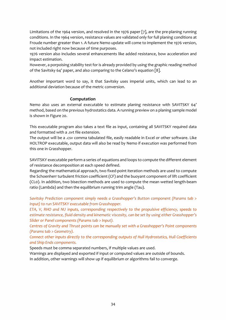
Computation Nemo also uses an external executable to estimate planing resistance with SAVITSKY 64’ method, based on the previous hydrostatics data. A running preview on a planing sample model is shown in Figure 20. This executable program also takes a text file as input, containing all SAVITSKY required data and formatted with a .svt file extension. The output will be a .csv comma tabulated file, easily readable in Excel or other software. Like HOLTROP executable, output data will also be read by Nemo if execution was performed from this one in Grasshopper. SAVITSKY executable perform a series of equations and loops to compute the different element of resistance decomposition at each speed defined. Regarding the mathematical approach, two fixed-point iteration methods are used to compute the Schoenherr turbulent friction coefficient (CF) and the buoyant component of lift coefficient (CL0). In addition, two bisection methods are used to compute the mean wetted length-beam ratio (Lambda) and then the equilibrium running trim angle (Tau). Savitsky Prediction component simply needs a Grasshopper’s Button component (Params tab > Input) to run SAVITSKY executable from Grasshopper. ETA, V, RHO and NU inputs, corresponding respectively to the propulsive efficiency, speeds to estimate resistance, fluid density and kinematic viscosity, can be set by using either Grasshopper’s Slider or Panel components (Params tab > Input). Centres of Gravity and Thrust points can be manually set with a Grasshopper’s Point components (Params tab > Geometry). Connect other inputs directly to the corresponding outputs of Hull Hydrostatics, Hull Coefficients and Ship Ends components. Speeds must be comma separated numbers, if multiple values are used. Warnings are displayed and exported if input or computed values are outside of bounds. In addition, other warnings will show up if equilibrium or algorithms fail to converge.

35

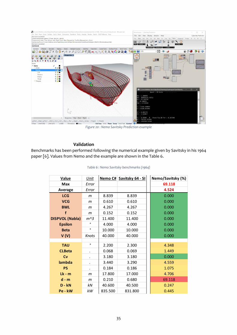
Figure 20 : Nemo Savitsky Prediction example

Validation Benchmarks has been performed following the numerical example given by Savitsky in his 1964 paper [6]. Values from Nemo and the example are shown in the Table 6.

Table 6 : Nemo Savitsky benchmarks (1964)

Value Unit Nemo C# Savitsky 64 - SI Nemo/Savitsky (%)Max Error 69.118

Average Error 4.524LCG m 8.839 8.839 0.000VCG m 0.610 0.610 0.000BWL m 4.267 4.267 0.000

f m 0.152 0.152 0.000DISPVOL (Nabla) m^3 11.400 11.400 0.000

Epsilon ° 4.000 4.000 0.000Beta ° 10.000 10.000 0.000V (V) Knots 40.000 40.000 0.000

TAU ° 2.200 2.300 4.348CLBeta . 0.068 0.069 1.449

Cv . 3.180 3.180 0.000lambda . 3.440 3.290 4.559

PS . 0.184 0.186 1.075Lk - m m 17.800 17.000 4.706d - m m 0.210 0.680 69.118D - kN kN 40.600 40.500 0.247

Pe - kW kW 835.500 831.800 0.445

36

Maximum deviation is the vertical depth of trailing edge of boat at keel below level water surface (d). Explanation of this difference comes out from the fact that equilibrium angle (TAU) found by NEMO is probably a way more accurate than the analytical and manual resolution computed by Savitsky by hand. Considering this last observation, the results appears reliable and acceptable, before a next upgrade with the 1976 version. A further test on a 3D model will be useful to do, as well as a new series when will be done.

C. NavCad Export Format hydrostatics data to export to NAVCAD (resistance prediction and power estimate analysis software). Nemo provides a NavCad Export component, to format hydrostatics data into a NAVCAD project file, readable since 2013 version (either licensed or demo version). This file is in fact a JSON format. Most of the inputs are set using the corresponding outputs of Hull Hydrostatics, Hull Coefficients, Ship Silhouette and Ship Ends components. Centres of Gravity and Thrust points can be manually set with a Grasshopper’s Point components (Params tab > Geometry). Grasshopper’s Panel components (Params tab > Input) are used to define kinematic viscosity value, and FilePath to save the NAVCAD .hcnc exported file. Two Grasshopper’s Toggle components (Params tab > Input) defines whether if model is a monohull (False) or a catamaran (True), and if hard chine is present (True) or not (False). Finally, a simple Grasshopper’s Button (Params tab > Input) is used to run the export process.

37

VII. Nemo: Meshing This final part explains the meshing capabilities provided with Nemo and Plankton library, that can then be used to run flow simulations or specific clean mesh exports. Plankton library, from Daniel Piker and Will Pearson, is a C# half-edge mesh data structure and components for using this in Grasshopper / Rhino. It allows in Nemo’s case, the generation of clean hull surface meshes by relaxing cells iteratively to get more uniform distributed triangles. Plankton also offers an option to refine locally following curvature areas, and maintain the edges position (extremely useful in case of hard chine). New Rhino quad mesher could be added in a next upgrade of Nemo, when this command will be available outside Rhino WIP. Flow simulations can be directly run using Cherie executable. Export files and settings can be directly driven from Nemo, or manually set using a simple copy-paste and file editing procedure. An additional export has also been added for MCC software.

A. Hull Mesh To generate a surface mesh for the hull, the procedure is as follows: Mesh hull geometry in more uniform triangles, keep hard edges, cut at specified height to mesh only interesting part, and refine on curvature. Hull MeshPlankton component computes advanced actions to generate mesh, extracts specific points from transom, keeps edges and repairs vertices position. Figure 21 shows a surface mesh of the portside part of DTMB model, cut at 75 mm above waterplane, and without refinement. Depending of the geometry used, simple or complex, clean or mess, the mesh generation can fail. Playing with settings combination usually resolves the issue, in particular the IterationsNb which has a big impact (start with a low iteration number, then once other desired settings are set and working, increase iterations progressively until best relaxation pattern). Connect the hull geometry to mesh, either by using a Grasshopper’s Brep component (Params tab > Geometry), or directly from the HullMesh output of Ship Import component. Transom geometry is used to extract transom id, which is then used for some external flow simulation software. These vertices are displayed as numbered dots (t.x, where x is the transom points number), and vertices id are given in output. Connect Transom input in the same way, either by using a Grasshopper’s Brep component (Params tab > Geometry), or directly from the Transom output of Ship Import component. CutHull input defines if the entire hull geometry will be meshed (False) or only the part below CutOffset height (True). Connect a Grasshopper’s Toggle component (Params tab > Input). CutOffset is a Z height from flotation level. Other inputs are set using Grasshopper’s Slider components (Params tab > Input). MeshLength is the required typical length of a triangle edge, the value is a percentage of LOA. MeshRefine allows refinement in high curvature areas, this setting is a simple percentage value (0 = no refinement, 100 = maximum refinement).

38

IterationsNb is the number of relaxation loops to smooth the mesh and converge towards a uniform repartition of triangles (greater number more regular the triangles will be). Tolerance sets the distance value for vertices remapped on X and Y axis (if vertices are within this tolerance distance, it will be move to X = 0 or Y = 0). Remapped vertices are displayed as red dots for X moves, and green dots for Y moves. HullNb is a counter used for some external flow simulation software, giving the number of hull meshed (useful if working on multihull cases).

Figure 21 : Hull MeshPlankton example

B. Cherie Simulation CHERIE software (Hydrodynamic Code for Evaluation of Flow-induced Resistance) is a potential flow simulation code that estimates the wave resistance of a ship using Dawson's model resolution, developed by the DGA. The main input file is a mesh of the hull, while the free surface around the hull is directly meshed by CHERIE. The second input file specifies simulation settings, in particular ship speeds as well as many parameters that control the positioning, free surface mesh and simulation conditions. Among the viscous effects, only the friction forces are taken into account. Nemo provides specific components to export these input files and run CHERIE simulations. After the generation of the hull mesh with Hull MeshPlankton component, a positioning transformation is required to respect CHERIE conventions. CHERIE use a specific (and unfortunately different) convention from Nemo. Backward is positive X, Up is positive Z, and Rhino XY world plane is the flotation level. Meaning the mesh used by CHERIE must be starboard side in Positive Y, X = 0 the bow of the ship.

39

Transom id also need specific order. First transom id is the Y and Z top most point, then follows the transom curve from deck edge on starboard to central axis Y = 0 (this one will be the last point). Last consideration is about mesh’s normals. Like in Ship Import component, they need to be correctly oriented, pointing out, looking to the exterior of the mesh (towards the water). Cherie Orient component will transform the existing mesh from Hull MeshPlankton to CHERIE convention. Figure 22 shows the new mesh orientation. Connect Grasshopper’s Toggle components (Params tab > Input), and same corresponding inputs to Hull MeshPlankton outputs.

ReOrient is used to flip the mesh orientation back to forth, PortSide to flip mesh over X axis, and FlipNormals, as it says, is to flip mesh’s normals. Regarding Transom id, if order is going in the wrong way, simply Right-Click on Transom Id input and select Reverse option to flip the order.

Figure 22 : Cherie Orient example

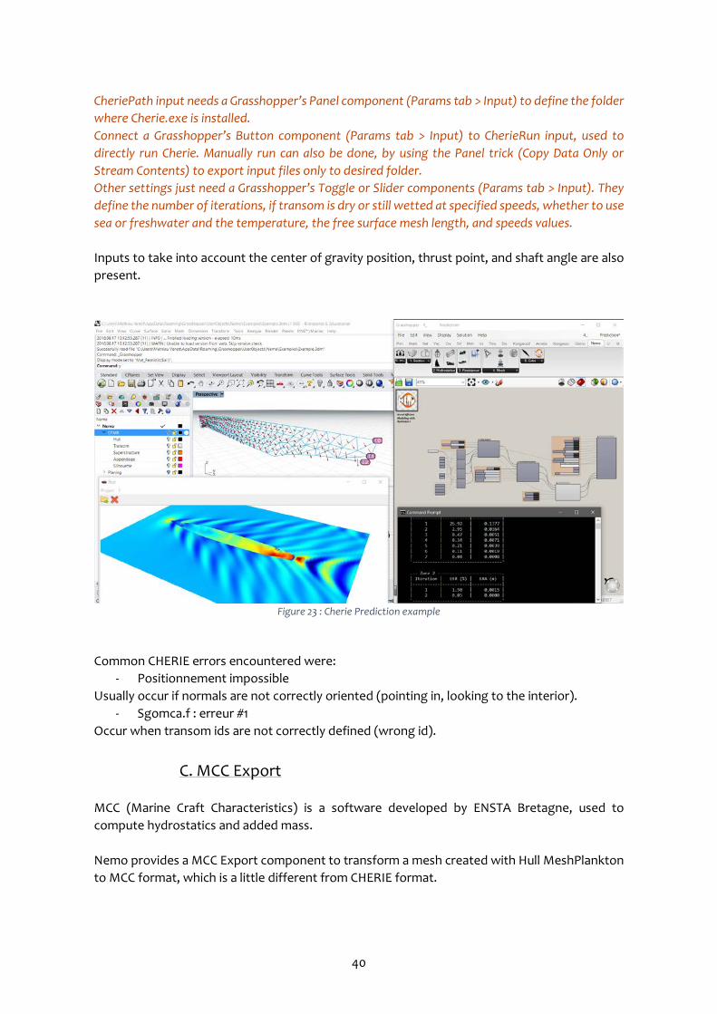
Once mesh is correctly oriented, Cherie Prediction component can be used to define basic simulation settings, export input files, and directly run CHERIE simulation from within Grasshopper. Figure 23 show an example of the workflow between Nemo, CHERIE and display.

40

CheriePath input needs a Grasshopper’s Panel component (Params tab > Input) to define the folder where Cherie.exe is installed. Connect a Grasshopper’s Button component (Params tab > Input) to CherieRun input, used to directly run Cherie. Manually run can also be done, by using the Panel trick (Copy Data Only or Stream Contents) to export input files only to desired folder. Other settings just need a Grasshopper’s Toggle or Slider components (Params tab > Input). They define the number of iterations, if transom is dry or still wetted at specified speeds, whether to use sea or freshwater and the temperature, the free surface mesh length, and speeds values. Inputs to take into account the center of gravity position, thrust point, and shaft angle are also present.

Figure 23 : Cherie Prediction example

Common CHERIE errors encountered were:

- Positionnement impossible Usually occur if normals are not correctly oriented (pointing in, looking to the interior).

- Sgomca.f : erreur #1 Occur when transom ids are not correctly defined (wrong id).

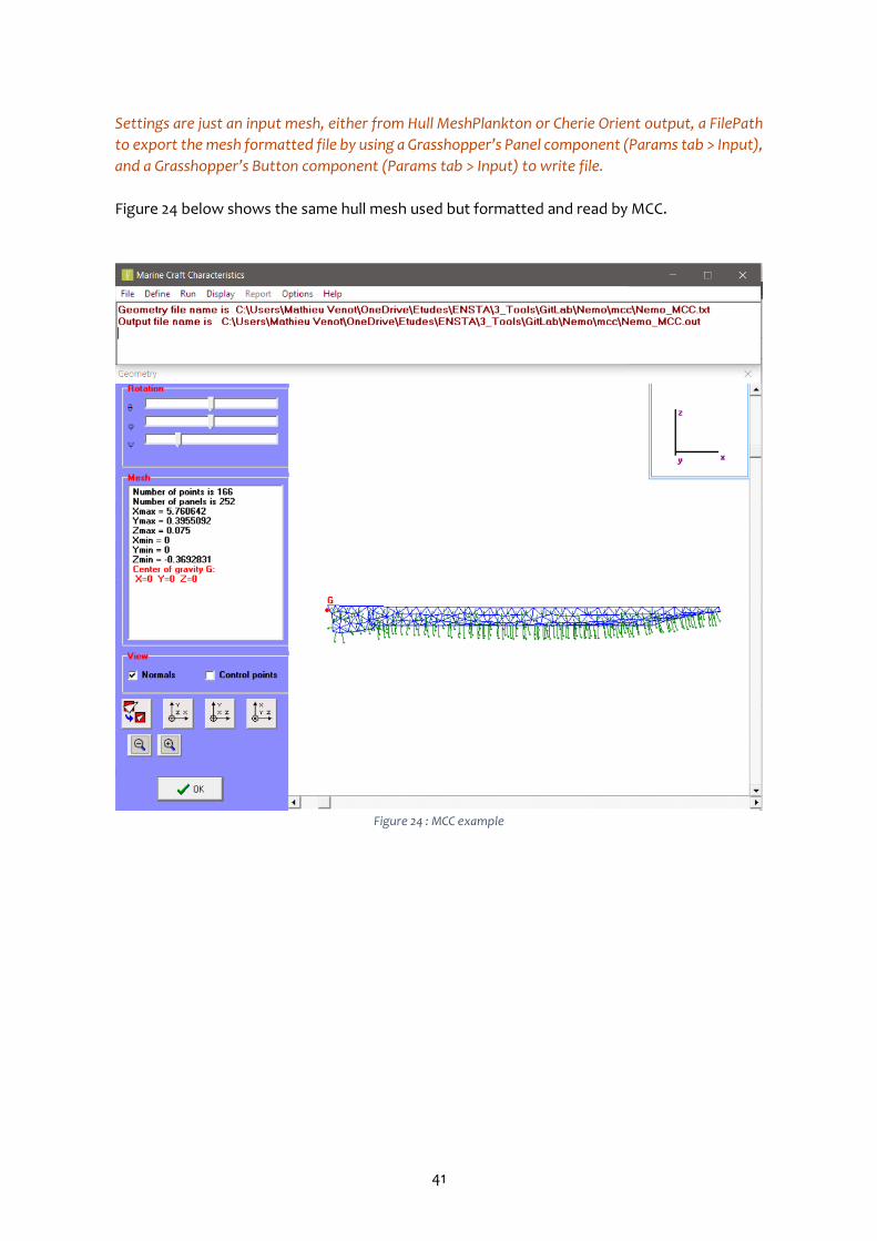
C. MCC Export MCC (Marine Craft Characteristics) is a software developed by ENSTA Bretagne, used to compute hydrostatics and added mass. Nemo provides a MCC Export component to transform a mesh created with Hull MeshPlankton to MCC format, which is a little different from CHERIE format.

41

Settings are just an input mesh, either from Hull MeshPlankton or Cherie Orient output, a FilePath to export the mesh formatted file by using a Grasshopper’s Panel component (Params tab > Input), and a Grasshopper’s Button component (Params tab > Input) to write file. Figure 24 below shows the same hull mesh used but formatted and read by MCC.

Figure 24 : MCC example

42

VIII. Conclusion Ship design and building industries are professional fields where execution times are very short. Conception by the architect and construction by the shipyard require constant exchanges that needs to be efficient to minimize impact on study and delivery times. In this context, whereas a lot of leading software brands try to impose their own all-in-one solutions, Nemo shows the opposite philosophy by reflecting the desire to link independent software. Many software are often dedicated to specialized tasks, so why trying to remake or replace an already existing good working solution ? Nemo brings a package of tools to communicate, exchange and benefit of such powerful external software. In addition, it also provides integrated functions for common uses of the architect. All these development steps, between hydrostatics – resistance – meshing – and additional tools computations, should expose how great open minded software Rhino and his environment are. Benchmarks performed confirm Nemo’s reliability according to the values computed. Even more, deviations obtained are often positive errors, considering the NURBS computation done by Nemo over other software tested who use meshed geometry. However, important limitation because of the NURBS computation, is the speed and time consuming which are quite constraining. Otherwise, SAVITSKY method still needs further work to take into account pre-planing conditions and a new run of comparisons will need to be done. In spite of that, Windows and Rhino 5 / 6 / WIP compatibility is full supported. Mac compatibility is not fully assumed but might partially work, and full support will be added later. For now, Nemo 1.0 Beta version has been released. Feedback and suggestions will be an important step in the future, to debug and optimize it before releasing new ones with enhanced and new features. Such new features already in mind, are to upgrade Nemo with stability analysis modules, parametric design assistants (for hulls, blades and appendages), integration of SAVITSKY 1976 method, better understanding of errors and warnings returned, export of summary or report file, new meshing pattern using quad cells, or even Excel interoperability for weight estimate linking. As a first series of adventures, Nemo should be used by the ENSTA Bretagne students next year, on a 2 months course about designing a patrol or passenger boat. This will be the first big swim for Nemo !

43

Troubleshooting Some tips for Grasshopper are presented here, to explain basic logic, simple actions and helpful components to use with Nemo. A known issues section is also presented, as Nemo is in continuous development, some constraints or problems can still persist. This section explains how to resolve or avoid it.

Grasshopper Tips Some quick tips and useful actions are presented here, based on Grasshopper core features able to enhance Nemo’s experience.

- Speed improvement (Right-Click and select Enabled) As Nemo calculations are made over NURBS geometry directly, time consuming could be important. By Right-Click a Nemo component, Enabled option can be used to switch between activated or deactivated states to activate or stop the component’s computation. By Right-Click on Grasshopper’s canvas, Lock Solver option can also be used to stop computations while editing Nemo’s settings.

- Input types (Typed data) Each component is data typed to know which kind of data can be used. This data type is representing as an icon in Grasshopper, corresponding to the ones present in Params tab. In most cases, Nemo has many input names followed by a _xxx where xxx is the data type abbreviation.

- Bake geometry (Right-Click and select Bake) Nemo’s geometry is compute as Grasshopper ghost geometry, meaning that this geometry is not living physically in Rhino. To transfer this ghost geometry to Rhino, the process is called Baking. By Right-Click on any component displaying geometry, Bake option should appear, then asking on which Rhino layer the component’s ghost geometry will be copied to become physical in Rhino. Another more advanced Baking process is possible using the Grasshopper’s Geometry Cache component (Params tab > Geometry), to continuously bake the geometry into the specified Rhino layer.

- Brep component (Params tab > Geometry) Always used to import geometry to Nemo. By Right-Click on it, select Set Multiple Breps and select the geometry into Rhino viewport, tape enter to validate. Beware to correctly organize branches if using multihull geometry (using Graft + Simplify options on inputs or outputs).

44

Another more advanced import process is possible using the Grasshopper’s Geometry Pipeline component (Params tab > Geometry), to continuously take the geometry from a specified Rhino layer.

- Panel component (Params tab > Input) The Panel is very useful to display and extract data, by visualizing the branches organization and data type. By Right-Click on it, Copy Data Only option can be used to simply copy-paste any type of data displayed. In Nemo’s case, it could be used for example to manually edit the Holtrop, Savitsky or Cherie files. By Right-Click on it, Stream Contents option can be used to continuously write into a file. May be used for example for seamless workflow with Holtrop, Savitsky or Cherie files and running the executables manually.

- Explode Tree component (Sets > Tree) Useful to quickly dispatch data contained in multiple branches, by Right-Click on it and select Match Outputs option. This trick is used in combination with the Panel component to copy-paste successively the list of points to MARS2000.

- Button component (Params tab > Input) The Button is used to run Windows executables, especially Holtrop, Savitsky and Cherie codes. To run it manually, simply copy-paste data into files using the Panel trick, files must be in the same directory as the executable, then run it manually from Windows Explorer or Command Prompt. For a quick start about Grasshopper, presenting a more detailed overview of the previous tips discussed, please refer to the [18] and [19] links.

Known Issues As explained before, Nemo is continuously growing up, and imperfections can be present. Here is a quick listing of identified problems that could occur, and solutions to solve the issues. Hydrostatics

- Flotation split fail: Hull splitting for below water computations can fail if hard chine is present and aligned all along with flotation level (Rhino XY world plane). >> Simply move up or down the entire model by just 1 mm. Resistances

- Running executables freeze Rhino / Grasshopper: Running Windows executables when clicking the Button components will freeze Rhino / Grasshopper until the user manually close the Command Prompt window. >> Simply close Command Prompt window.

45

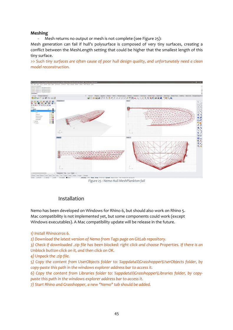
Meshing - Mesh returns no output or mesh is not complete (see Figure 25):

Mesh generation can fail if hull’s polysurface is composed of very tiny surfaces, creating a conflict between the MeshLength setting that could be higher that the smallest length of this tiny surface. >> Such tiny surfaces are often cause of poor hull design quality, and unfortunately need a clean model reconstruction.

Figure 25 : Nemo Hull MeshPlankton fail

Installation Nemo has been developed on Windows for Rhino 6, but should also work on Rhino 5. Mac compatibility is not implemented yet, but some components could work (except Windows executables). A Mac compatibility update will be release in the future. 1) Install Rhinoceros 6. 2) Download the latest version of Nemo from Tags page on GitLab repository. 3) Check if downloaded .zip file has been blocked: right click and choose Properties. If there is an Unblock button click on it, and then click on OK. 4) Unpack the .zip file. 5) Copy the content from UserObjects folder to: %appdata%\Grasshopper\UserObjects folder, by copy-paste this path in the windows explorer address bar to access it. 6) Copy the content from Libraries folder to: %appdata%\Grasshopper\Libraries folder, by copy-paste this path in the windows explorer address bar to access it. 7) Start Rhino and Grasshopper, a new "Nemo" tab should be added.

46

References 1. Holtrop, J., “A Statistical Analysis of Performance Test Results”, International Shipbuilding Progress, Vol. 24, February 1977 2. Holtrop, J. and Mennen, G.G.J., “A Statistical Power Prediction Method”, International Shipbuilding Progress, Vol. 25, October 1978 3. Holtrop, J. and Mennen, G.G.J., “An Approximate Power Prediction Method”, International Shipbuilding Progress, Vol. 29, July 1982 4. Holtrop, J., “A Statistical Re-Analysis of Resistance and Propulsion Data”, International Shipbuilding Progress, Vol. 31, November 1984 5. Holtrop, J., “A Statistical Resistance Prediction Method with a Speed Dependent Form Factor”, SMSSH ‘88, October 1988 6. Savitsky, D., “Hydrodynamic Design of Planing Hulls”, SNAME Marine Technology, October 1964 7. Savitsky, D. and Brown, P.W, “Procedures for Hydrodynamic Evaluation of Planing Hulls in Smooth and Rough Water”, Marine Technology, Vol. 13, October 1976 8. Celano, T., “The Prediction of Porpoising Inception for Modern Planing Craft”, U.S.N.A. - Trident Scholar project report, 1998 9. Abbott, I.H., Von Doenhoff, E., Theory of Wing Sections: Including a Summary of Airfoil Data, Dover Publications, June 1959 10. Paulet, D. and Presles, D., “Architecture Navale - Connaissance et Pratique”, Editions De La Villette, December 1998 11. Laurens, J-M., Doutreleau, Y. and Jodet, L., “Résistance et Propulsion du Navire : Résistance à l'Avancement, Hélice, Appareil Propulsif”, Ellipses Technosup, May 2011 12. Laurens, J-M. and Grinnaert, F., “Stabilité du Navire : Théorie, Réglementation, Méthodes de Calcul”, Ellipses Technosup, June 2013 13. Biran, A. and Lopez-Pulido, R., “Ship Hydrostatics and Stability”, Butterworth-Heinemann, October 2013 14. Bertram, V., “Practical Ship Hydrodynamics”, Elsevier, September 2011 15. Faltinsen, O.M., “Hydrodynamics of High-Speed Marine Vehicles”, Cambridge University Press, January 2006 16. ITTC, “ITTC Symbols and Terminology List”, September 2011 17. ITTC, “Dictionary of Hydromechanics”, August 2011 18. Jeffries, P., A beginner’s guide to visual scripting with Grasshopper, http://blog.ramboll.com/rcd/tutorials/a-beginners-guide-to-visual-scripting-with-grasshopper.html, October 2017 19. TU Delft, Grasshopper, http://wiki.bk.tudelft.nl/toi-pedia/Grasshopper, July 2018