Neighbor list collision-driven molecular dynamics simulation for nonspherical hard particles. I....
28
Neighbor list collision-driven molecular dynamics simulation for nonspherical hard particles. I. Algorithmic details Aleksandar Donev a,b , Salvatore Torquato a,b,c, * , Frank H. Stillinger c a Program in Applied and Computational Mathematics, Princeton University, Princeton, NJ 08544, USA b Princeton Institute for the Science and Technology of Materials, Princeton University, Princeton, NJ 08540, USA c Department of Chemistry, Princeton University, Princeton, NJ 08540, USA Received in revised form 19 May 2004; accepted 9 August 2004 Available online 11 November 2004 Abstract In this first part of a series of two papers, we present in considerable detail a collision-driven molecular dynamics algorithm for a system of non-spherical particles, within a parallelepiped simulation domain, under both periodic or hard-wall boundary conditions. The algorithm extends previous event-driven molecular dynamics algorithms for spheres, and is most efficient when applied to systems of particles with relatively small aspect ratios and with small variations in size. We present a novel partial-update near-neighbor list (NNL) algorithm that is superior to previous algorithms at high densities, without compromising the correctness of the algorithm. This efficiency of the algorithm is further increased for systems of very aspherical particles by using bounding sphere complexes (BSC). These tech- niques will be useful in any particle-based simulation, including Monte Carlo and time-driven molecular dynamics. Additionally, we allow for a non-vanishing rate of deformation of the boundary, which can be used to model macro- scopic strain and also alleviate boundary effects for small systems. In the second part of this series of papers we spe- cialize the algorithm to systems of ellipses and ellipsoids and present performance results for our implementation, demonstrating the practical utility of the algorithm. Ó 2004 Elsevier Inc. All rights reserved. 1. Introduction Classical molecular dynamics (MD) simulations have been used to study the properties of particle sys- tems for many decades. The first MD studies used the simplest multi-particle system, the hard-sphere fluid/ 0021-9991/$ - see front matter Ó 2004 Elsevier Inc. All rights reserved. doi:10.1016/j.jcp.2004.08.014 * Corresponding author. Tel.: +1 609 258 3341; fax: +1 609 258 6878. E-mail address: [email protected] (S. Torquato). Journal of Computational Physics 202 (2005) 737–764 www.elsevier.com/locate/jcp
-
Upload
aleksandar-donev -
Category
Documents
-
view
214 -
download
0
Transcript of Neighbor list collision-driven molecular dynamics simulation for nonspherical hard particles. I....

Journal of Computational Physics 202 (2005) 737–764
www.elsevier.com/locate/jcp
Neighbor list collision-driven molecular dynamics simulationfor nonspherical hard particles. I. Algorithmic details
Aleksandar Donev a,b, Salvatore Torquato a,b,c,*, Frank H. Stillinger c
a Program in Applied and Computational Mathematics, Princeton University, Princeton, NJ 08544, USAb Princeton Institute for the Science and Technology of Materials, Princeton University, Princeton, NJ 08540, USA
c Department of Chemistry, Princeton University, Princeton, NJ 08540, USA
Received in revised form 19 May 2004; accepted 9 August 2004
Available online 11 November 2004
Abstract
In this first part of a series of two papers, we present in considerable detail a collision-driven molecular dynamics
algorithm for a system of non-spherical particles, within a parallelepiped simulation domain, under both periodic or
hard-wall boundary conditions. The algorithm extends previous event-driven molecular dynamics algorithms for
spheres, and is most efficient when applied to systems of particles with relatively small aspect ratios and with small
variations in size. We present a novel partial-update near-neighbor list (NNL) algorithm that is superior to previous
algorithms at high densities, without compromising the correctness of the algorithm. This efficiency of the algorithm
is further increased for systems of very aspherical particles by using bounding sphere complexes (BSC). These tech-
niques will be useful in any particle-based simulation, including Monte Carlo and time-driven molecular dynamics.
Additionally, we allow for a non-vanishing rate of deformation of the boundary, which can be used to model macro-
scopic strain and also alleviate boundary effects for small systems. In the second part of this series of papers we spe-
cialize the algorithm to systems of ellipses and ellipsoids and present performance results for our implementation,
demonstrating the practical utility of the algorithm.
� 2004 Elsevier Inc. All rights reserved.
1. Introduction
Classical molecular dynamics (MD) simulations have been used to study the properties of particle sys-tems for many decades. The first MD studies used the simplest multi-particle system, the hard-sphere fluid/
0021-9991/$ - see front matter � 2004 Elsevier Inc. All rights reserved.
doi:10.1016/j.jcp.2004.08.014
* Corresponding author. Tel.: +1 609 258 3341; fax: +1 609 258 6878.
E-mail address: [email protected] (S. Torquato).

738 A. Donev et al. / Journal of Computational Physics 202 (2005) 737–764
solid [1], which is very rich in behavior. Subsequently, methods were developed to follow the dynamics of a
system of soft spheres, i.e., particles interacting with a spherically symmetric and continuous interparticle
potential, usually with a hard cutoff on the range of the interaction. The algorithms needed to simulate the
two types of systems are rather different, and difficult to combine [12]. For soft particles, one needs to inte-
grate a system of ordinary differential equations given by Newton�s law of motion. However, for hard par-ticles the interaction potential is singular and the task of integrating the equations of motion becomes a
problem of processing a sequence of binary collisions between the particles, 1 or collisions of the particles
with the hard walls of a container, if any. In other words, for hard particles, one needs to predict and
process a sequence of discrete events of vanishing duration.
The algorithm for hard particles therefore becomes event-driven, as opposed to the time-driven algorithm
for soft-particle MD in which time changes in small steps and the equations of motion are integrated.
Event-driven algorithms have the task of scheduling a sequence of events predicted to happen in the future.
The simulation is advanced to the time of the event with the smallest scheduled time (the impending event)and that event is processed. The schedule of events is updated if necessary and the same process is repeated.
In molecular dynamics, the primary kind of event are binary collisions, so the simulation becomes collision-
driven. This kind of collision-driven approach was used for the very first MD simulation of the hard-disk
system [1], and has since been extended and improved in a variety of ways, most importantly, to increase the
efficiency of the algorithm. All of these improvements, namely, delayed particle updates, the cell method, the
use of a heap for the event queue, etc., appear in almost any efficient hard-particle MD algorithm. Systems
of many thousands of hard disks or spheres can be studied on a modern personal computer using such algo-
rithms, and in the past decade the method has been extended to handle more complex simulations, such asparticles in a velocity field [30].
However, we are aware of only one collision-driven simulation in the literature for non-spherical parti-
cles, namely, one for very thin rods (needles) [8]. Other molecular dynamics simulations for hard non-spher-
ical particles have used a time-driven approach [2], which is simpler to implement than the event-driven
approach but inferior in both accuracy and efficiency (at high densities). Two kinds of smooth shapes
are used frequently to model aspherical particles: spherocylinders (a cylinder with two spherical caps),
and ellipsoids. Both can become spheres in a suitable limit. Spherocylinders are analytically much simpler
then ellipsoids, however, they are always axisymmetric and cannot be oblate.The primary reason event-driven algorithms have not yet been used for non-spherical particles is that a
high-accuracy collision-driven scheme for non-trivial particle shapes and sufficiently large systems is very
demanding. Computers have only recently reached the necessary speeds, and a proper implementation in-
volves a significant level of code complexity. In this paper, we present in detail a collision-driven molecular
dynamics algorithm for a system of hard non-spherical particles. The algorithm is based on previous event-
driven MD approaches for spheres, and in particular the algorithms of Lubachevsky [19] and Sigurgeirsson
et al. [2]. While in principle the algorithm is applicable to any particle shape, we have specifically tailored it
for smooth particles for which it is possible to introduce and easily evaluate continuously differentiableoverlap potentials. Additionally, it is assumed that the particles have a spherically symmetric moment of
inertia, so that in-between collisions their angular velocities are constant. Furthermore, the algorithm is
most efficient when applied to relatively dense and homogeneous systems of particles which do not differ
widely in size (i.e., the degree of polydispersity is small). We focus in this work on systems with lattice-based
boundaries, under both periodic or hard-wall boundary conditions. The main innovations and strengths of
the proposed algorithm are:
1 Multi-particle collisions have zero probability of occurring and will not be considered here.

A. Donev et al. / Journal of Computational Physics 202 (2005) 737–764 739
� It specifically allows for non-axially symmetric particles by using quaternions in the representation of
orientational degrees of freedom, unlike previous hard-particle algorithms which have been restricted
just to needles, spherocylinders or spheroids.
� The particle-shape-dependent components of the algorithm are clearly separated from general concepts,
so that it is (at least in principle) easy to adapt the algorithm to different particle shapes. In the secondpart of this series of papers we present in detail the implementation of these components for ellipses and
ellipsoids.
� It explicitly allows for time-dependent particle shapes and for time-dependent shape of the boundary
cell, which enables a range of non-equilibrium applications and also Parinello–Rahman-like [26] con-
stant-pressure molecular dynamics.
� It corrects some assumptions in traditional hard-sphere algorithms that are not correct for non-spherical
particles or when boundary deformation is included, such as the nearest image convention in periodic sys-
tems and the claim that there must be an intervening collision between successive collisions of a givenpair of particles.
� It is the first rigorous event-driven MD algorithm to incorporate near-neighbor lists, by using the concept
of bounding neighborhoods. This is a very significant improvement for very aspherical particles and/or at
high densities, and has some advantages over the traditional cell method even for hard spheres because it
allows a close monitoring of the collision history of the algorithm.
� It is the first algorithm to specifically address the problem of efficient near-neighbor search for very elon-
gated or very flat particles by introducing the concept of bounding sphere complexes. The algorithm also
clearly separates neighbor-search in a static environment (where particle positions are fixed) from its usein a dynamic environment (where particles move continuously), thus enabling one to easily incorporate
additional neighbor search techniques. We emphasize that the developed near neighbor search tech-
niques will improve all particle-based simulations, including Monte Carlo and time-driven molecular
dynamics.
� It is documented in detail with pseudo-codes which closely follow the actual Fortran 95 code used to
implement it for ellipses and ellipsoids.
One motivation for developing this algorithm has been to extend the Lubachevsky–Stillinger sphere-packing algorithm [20,21] to non-spherical particles. We have successfully used our implementation to ob-
tain many interesting results for random and ordered packings of ellipses and ellipsoids [6]. The algorithm
can also be used to study equilibrium properties of hard-ellipse and hard-ellipsoid systems, and we give sev-
eral illustrative applications in the second paper of this series. In the second paper we also numerically dem-
onstrate that our novel neighbor-search techniques can speed the simulation by as much as two orders of
magnitude or more at high densities and/or for very aspherical particles, as compared to direct adaptations
of traditional hard-sphere schemes.
We begin by presenting preliminary information and the basic ideas behind the algorithm in Section 2.We then focus on the important task of improving the efficiency of the algorithm by focusing on neighbor
search in Section 3, and present both the classical cell method and our adaptation of near-neighbor lists.
Detailed pseudo-codes for all major steps in the algorithm for general non-spherical particles are given
in Section 4, and these are continued in the second part of this series of papers for the specific case of
ellipses and ellipsoids.
2. Preliminaries
In this section, we give some background information and a preliminary description of the algorithm.
First, we discuss the impact the shape of the particles has on the algorithm. Then, we briefly describe

740 A. Donev et al. / Journal of Computational Physics 202 (2005) 737–764
the two main approaches to hard-particle molecular dynamics, time-driven and event-driven. Finally, we
discuss boundary conditions in our event-driven molecular dynamics algorithm and also the possibility
of performing event-driven MD in different ensembles. Bold symbols are reserved for vectors and matrices,
and subscripts are used to denote their components. Matrix multiplication is assumed whenever products of
matrices or a matrix and a vector appear. Subscripts or superscripts are used heavily to add specificity tovarious quantities, for example, r denotes position, while rA denotes the position of some particle A. We
denote the numerical precision with �� 1, and use subscripted ��s for various user-set (small) numerical
tolerances. We often omit explicit functional dependencies when they are clearly implied by the context
and it is not important to emphasize them, for example, f and f(t) will be used interchangeably.
2.1. Particle shape
We consider a system of N hard particles whose only interactions are given by impenetrability con-straints, although it is easy to allow for additional external fields which are independent of the particles
(such as gravity). Many of the techniques developed here are also used to deal with particles interacting
with a soft potential if there is a hard cutoff on the potential. We discuss the special case of orientation-less
particles, namely spheres, at length, and we use hard ellipsoids to illustrate the extensions to non-spherical
particles. We will use the terms sphere and ellipsoid in any dimension, but sometimes we will be more spe-
cific and distinguish between disk and ellipse in two dimensions, and sphere and ellipsoid in three
dimensions.
Spheres are a very important special case not only because of their simplicity, but also because boundingspheres are a necessary ingredient when dealing with aspherical particles. A bounding sphere for a particle is
centered at the centroid of the particle and has the minimal possible diameter Dmax = 2Omax so that it fully
encloses the particle itself. Here by centroid we mean a geometrically special point chosen so that the
bounding sphere is as small as possible (i.e., it should be chosen to be as close as possible to the midpoint
of the longest line segment joining two points of the particle). For example, for an ellipsoid, the bounding
sphere has the same center as the ellipsoid and its diameter is equal to the largest axes of the ellipsoid. The
importance of bounding spheres is that they provide a quick and analytically simple way to test for overlap
of two particles: Two particles cannot overlap if their bounding spheres do not overlap. Occasionally wemake use of contained spheres, which are also centered at the centroid of the particle and have the maximal
possible diameter Dmin = 2Omin so that they are fully within the particle itself. For ellipsoids their diameter
is the smallest axes. Note that two particles must overlap if their contained spheres overlap. The efficiency
of the EDMD algorithm described in this paper is primarily determined by the aspect ratio a = Dmax/Dmin.
The greater the deviation of a from unity, the worse the efficiency because the bounding/contained spheres
become worse approximations for the particles and because of the increasing importance of particle orien-
tations. We propose a novel near-neighbor list technique for dealing with very aspherical particles, in addi-
tion to the standard cell method.
2.2. Molecular dynamics
The goal of our algorithm is to simulate the motion of the particles in time as efficiently as possible, while
taking into account the interactions between the particles. For hard-particle systems, the only interactions
occur during binary collisions of the particles. The goal of hard-particle molecular dynamics (MD) algo-
rithms is to correctly predict the time-ordered sequence of particle collisions. Additionally, there may be
obstacles such as hard walls with which the particles can collide. Next, we briefly introduce the main ideasbehind the two main approaches to hard-particle MD, time-driven and event-driven MD. This preliminary
presentation will be helpful in understanding the rest of this section. Further details on the event-driven
algorithm are given in Section 4.
A. Donev et al. / Journal of Computational Physics 202 (2005) 737–764 741
2.2.1. Time driven MD
The time-driven molecular dynamics (TDMD) approach is inspired by MD simulations of systems of soft
particles (i.e., particles interacting with a continuous interaction potential). It has been adapted also to the
simulation of hard-particle systems, particularly non-spherical particles [2,28], mainly because of its sim-
plicity. In this approach, all of the particles are displaced synchronously in small time steps Dt and a checkfor overlap between the particles is done. If any two particles overlap, time is rolled back until the approx-
imate moment of initial overlap, i.e., the time of collision, and the collision of the particles is processed (i.e.,
the momenta of the colliding particles are updated), and the simulation continued. The main disadvantage
of this approach is that it is not rigorous, in the sense that collisions may be missed or the correct ordering
of a sequence of successive collisions may be mis-predicted (particularly in dense systems). To ensure a rea-
sonably correct prediction of the system dynamics, a very small time step must be used and this is ineffi-
cient. Nonetheless, since only checking for overlap between particles is needed, the simplicity of the
method is a very attractive feature. Additionally, such an approach is parallelizable with the sametechniques as any other MD algorithm (for example, domain decomposition).
2.2.2. Event driven MD
An alternative rigorous approach is to use event-driven molecular dynamics (EDMD), based on a rather
general model of discrete event-driven simulation. In EDMD, instead of advancing time independently of
the particles as in TDMD, time is advanced from one event to the next event, where an event is a binary
particle collision, or a collision of a particle with an obstacle (hard wall). Other types of events will be dis-
cussed shortly, however, collisions are the central type of event so we label the approach more specifically ascollision-driven molecular dynamics (CDMD). We will, however, continue to use the abbreviation EDMD
since the term event-driven is widely used in the literature.
Efficient implementations of EDMD are asynchronous: each particle is at the point in time when the last
event involving it happened. Each particle predicts what its impending event is and when it is expected to
happen. All of these events are entered into a priority event queue (typically implemented by a heap), which
allows for quick extraction of the next event to happen. The positions and momenta of the particles
involved in this event are updated, the particles� next event predicted, the event queue updated, and the sim-
ulation continued with the next event. Sometimes events may be mis-predicted. For example, a particle i
may predict a collision with particle j, but another (third party) particle m may collide with j before i
has time to. A special event called a check needs to be introduced, and it amounts to simply (re-)predicting
the impending event for a given particle. Given infinite numerical precision, this kind of approach rigor-
ously follows the dynamics of the system.
The computationally expensive step in EDMD is the prediction of the impending event of a given par-
ticle i (even though asymptotically the event-queue operations dominate). This typically involves the expen-
sive (especially for non-spherical particles) step of predicting the time of collision between the particle i and
a set of other particles j. In the simplest approach, one would predict the time of collision between i and allother particles and choose the smallest one, but a much more efficient approach is described in Section 3.
For spheres moving along straight lines, predicting the time of collision merely amounts to finding the first
positive root (if any) of a quadratic equation, and is very fast. Therefore, for spherical particles EDMD
always outperforms TDMD by orders of magnitude, and it is rigorous. For non-spherical particles, colli-
sion predictions are much more involved, but for algebraically simple smooth particle shapes it is expected
that EDMD will still outperform TDMD for a wide range of densities. Furthermore, there are systems for
which TDMD is not possible, and one must use EDMD, such as systems of hard line segments [8]. Note,
however, that the efficiency of the EDMD approach is possible only because the motion of the particlesbetween events can be predicted a priori, and because binary collisions only affect the two colliding parti-
cles. In cases when these assumptions are not true, TDMD may be the only option. Additionally, it is very
important to note that the EDMD algorithm is inherently non-parallelizable due its sequential processing

742 A. Donev et al. / Journal of Computational Physics 202 (2005) 737–764
of the events. Some attempts have been made to parallelize the method [18] by using the locality of the
interactions, and very recently actual implementations have appeared [24]. We will defer any discussion
of parallelization to future publications.
2.3. Boundary conditions
In this paper, we consider MD in a simple bounded simulation domain embedded in a Euclidean space
Ed of dimensionality d. In particular, we focus exclusively on lattice-based boundaries. This means that the
simulation domain, which the particles never leave, is a parallelepiped defined by d lattice vectors, k1,. . .,kd.The simulation domain, or unit cell, is a collection of points with d relative coordinates r in the interval [0,1],
and corresponding Cartesian coordinates
Fig. 1.
cell alo
(disk).
identifi
rðEÞ ¼Xd
k¼1rkkk ¼ Kr; ð1Þ
where K is a square invertible matrix representing the lattice, and contains the lattice vectors as columns.
The volume of the unit cell is given by the positive determinant |K|. As illustrated in Fig. 1(a), the param-
Illustration of lattice-based boundaries. The top subfigure shows a unit cell in two dimensions, along with the length of the unit
ng the x direction, L1, and the left and right ‘‘walls’’ along the x dimension. Also shown is a particle and its bounding sphere
The bottom subfigure shows a unit cell and an original particle (black), along with the first neighbor images and their image
ers v.
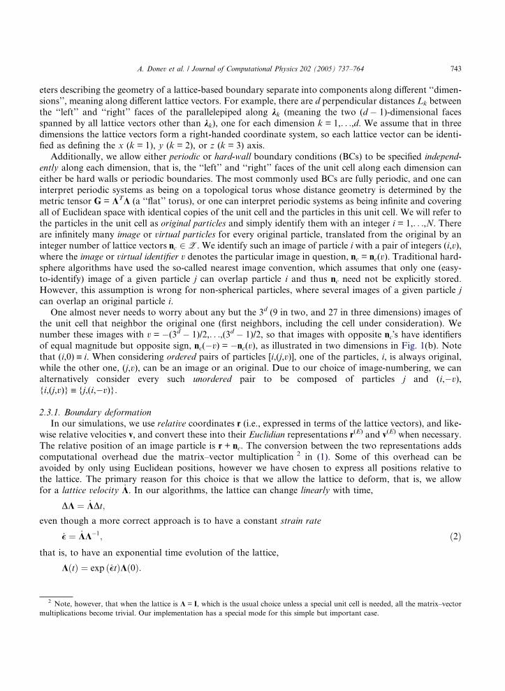
A. Donev et al. / Journal of Computational Physics 202 (2005) 737–764 743
eters describing the geometry of a lattice-based boundary separate into components along different ‘‘dimen-
sions’’, meaning along different lattice vectors. For example, there are d perpendicular distances Lk between
the ‘‘left’’ and ‘‘right’’ faces of the parallelepiped along kk (meaning the two (d � 1)-dimensional faces
spanned by all lattice vectors other than kk), one for each dimension k = 1,. . .,d. We assume that in three
dimensions the lattice vectors form a right-handed coordinate system, so each lattice vector can be identi-fied as defining the x (k = 1), y (k = 2), or z (k = 3) axis.
Additionally, we allow either periodic or hard-wall boundary conditions (BCs) to be specified independ-
ently along each dimension, that is, the ‘‘left’’ and ‘‘right’’ faces of the unit cell along each dimension can
either be hard walls or periodic boundaries. The most commonly used BCs are fully periodic, and one can
interpret periodic systems as being on a topological torus whose distance geometry is determined by the
metric tensor G = KTK (a ‘‘flat’’ torus), or one can interpret periodic systems as being infinite and covering
all of Euclidean space with identical copies of the unit cell and the particles in this unit cell. We will refer to
the particles in the unit cell as original particles and simply identify them with an integer i = 1,. . .,N. Thereare infinitely many image or virtual particles for every original particle, translated from the original by an
integer number of lattice vectors nc 2 Z. We identify such an image of particle i with a pair of integers (i,v),
where the image or virtual identifier v denotes the particular image in question, nc = nc(v). Traditional hard-
sphere algorithms have used the so-called nearest image convention, which assumes that only one (easy-
to-identify) image of a given particle j can overlap particle i and thus nc need not be explicitly stored.
However, this assumption is wrong for non-spherical particles, where several images of a given particle j
can overlap an original particle i.
One almost never needs to worry about any but the 3d (9 in two, and 27 in three dimensions) images ofthe unit cell that neighbor the original one (first neighbors, including the cell under consideration). We
number these images with v = �(3d � 1)/2,. . .,(3d � 1)/2, so that images with opposite nc�s have identifiers
of equal magnitude but opposite sign, nc(�v) = �nc(v), as illustrated in two dimensions in Fig. 1(b). Note
that (i,0) ” i. When considering ordered pairs of particles [i,(j,v)], one of the particles, i, is always original,
while the other one, (j,v), can be an image or an original. Due to our choice of image-numbering, we can
alternatively consider every such unordered pair to be composed of particles j and (i,�v),{i,(j,v)} ” {j,(i,�v)}.
2.3.1. Boundary deformation
In our simulations, we use relative coordinates r (i.e., expressed in terms of the lattice vectors), and like-
wise relative velocities v, and convert these into their Euclidian representations r(E) and v(E) when necessary.
The relative position of an image particle is r + nc. The conversion between the two representations adds
computational overhead due the matrix–vector multiplication 2 in (1). Some of this overhead can be
avoided by only using Euclidean positions, however we have chosen to express all positions relative to
the lattice. The primary reason for this choice is that we allow the lattice to deform, that is, we allow
for a lattice velocity _K. In our algorithms, the lattice can change linearly with time,
2 N
multip
DK ¼ _KDt;
even though a more correct approach is to have a constant strain rate
_� ¼ _KK�1; ð2Þ
that is, to have an exponential time evolution of the lattice,KðtÞ ¼ exp _�tð ÞKð0Þ:
ote, however, that when the lattice is K = I, which is the usual choice unless a special unit cell is needed, all the matrix–vector
lications become trivial. Our implementation has a special mode for this simple but important case.

744 A. Donev et al. / Journal of Computational Physics 202 (2005) 737–764
The identification of � = (DK)K�1 with the macroscopic strain is explained in [31], and we choose it to be
symmetric, _� ¼ _�T , to eliminate rotations of the unit cell.
In our approach, since the positions of the particles are relative to the lattice, the particles move together
with the lattice. This is necessary in order to simulate isotropic systems. Namely, had the positions of the
particles been independent of the lattice and the lattice deformed, for example, uniformly contracted, theimage particles would move with the lattice, but the originals would not, and this would lead to artificial
effects at the boundary of the unit cell. However, using relative positions is not without a cost. Consider a
particle at relative position r which moves with constant relative velocity v. Its Euclidean position is a
parabola
rðEÞðtÞ ¼ ðKþ _KtÞðrþ vtÞ ¼ Krþ ðKvþ _KrÞt þ ð2 _KvÞ t2
2; ð3Þ
rather than a straight line. We can identify the instantaneous Euclidean position and velocity as well as the
acceleration to be
rðEÞ ¼ Kr; ð4Þ
vðEÞ ¼ Kvþ _Kr; ð5Þ
aðEÞ ¼ 2 _Kv: ð6Þ
This complicates, for example, the calculation of the time of collision of two moving spherical particles.
Ordinarily a quadratic equation needs to be solved, but when the lattice deforms, a quartic equation needs
to be solved instead. To our knowledge, our algorithm is the first EDMD algorithm to include a deformingboundary.
In our algorithm, the lattice velocity is an externally imposed quantity, and our goal is to simulate the
motion of the particles as the boundary deforms, for example, in order to study shear banding in systems of
ellipsoids [10]. It is the usual case that the boundary deforms slowly compared to the motion of the parti-
cles. As the boundary deforms, the unit cell becomes less and less orthogonal, and so in long-time simula-
tions some form of orthogonalization of the unit cell might be necessary (we have not experimented with
such techniques). Previously used constant-shear MD techniques [17] do not have this problem, however
they are also not capable of simulating arbitrary shears and are plagued with boundary effects.Unlike in TDMD, in EDMD it is not possible to couple the motion of the boundary to all of the par-
ticles, as is done in Parinello–Rahman MD [26]. This is because the efficiency of the method depends crit-
ically on the fact that particles move independently between collisions and that particle collisions only affect
the colliding particles. However, a pseudo-PRMD approach is possible, in which the lattice velocity is
updated after a certain number of particle collisions, and the simulation is essentially restarted with a
new lattice velocity. We have some preliminary positive experience with such a method. Unit cell dynamics
is also needed to properly study anisotropic liquids, which is very important for non-spherical particles [15].
A deforming boundary can also be used to model macroscopic strain in multiscale simulations (for exam-ple, to simulate granular flow) in which microscale MD is used to obtain material properties needed for a
macroscopic continuum simulation.
2.4. EDMD in different ensembles
Molecular dynamics is often performed in ensembles different from the NVE one, and in particular,
constant temperature and constant pressure are often desired. For this purpose, various thermostats
have been developed. However, these are usually designed to be used with time-driven MD and systems

A. Donev et al. / Journal of Computational Physics 202 (2005) 737–764 745
of soft particles. We are in fact aware of no work that explicitly discusses thermostats for event-driven
MD.
Hard particle systems are inherently athermal due to the lack of energy scale, and the pressure and time
scaling are therefore arbitrary. Sophisticated temperature or pressure thermostats are thus not usually
needed. In particular, simple velocity rescaling can be used to keep the temperature at the desired value.The average translational kinetic energy Ek per particle can be calculated and then both the translational
and angular velocities scaled by the factor s ¼ffiffiffiffiffiffiffiffiffiffiffiffiffiffiffiffiffiffiffiffidkBT=2Ek
pand the simulation essentially restarted. 3 This
kind of temperature control is needed when, for example, the particles grow or shrink in size, since this
leads to non-conservative collision dynamics and an overall heating or cooling of the system. Although
velocity rescaling is simple and convenient, it has serious deficiencies [11], and a true canonical thermostat
may be needed in some applications. For this purpose, an Andersen thermostat [9] can be included in col-
lision-driven algorithms by considering the thermostat as a possible collision partner (with an appropriate
Poisson distribution of collision times). We do not include such a stochastic temperature thermostat in ouralgorithm explicitly, since we have not used it.
A Parinello–Rahman-like isostress (isopressure) thermostat [26] cannot be directly included in collision-
driven algorithms, since it implicitly couples the motion of all particles via the deformation of the unit cell
and thus destroys the asynchronous efficiency of collision-driven approaches. Such a thermostat is often
needed, even for hard particles, in simulations of crystal phases in order to keep the internal stress tensor
isotropic and to allow for changes of the crystal unit cell. We have used constant shear boundary deforma-
tions, as described in Section 2.3.1, to implement a partial isostress thermostat in which the shear rate is
periodically updated to reflect the asymmetry of the stress tensor. This approach has had a mixed successand additional work is required to improve it, especially for anisotropic systems of (aspherical) particles
[15].
3. Speeding up the search for neighbors
Identifying the near-neighbors of a given particle has the most important impact on efficiency in almost
all simulations of particle systems, particularly when the interparticle interactions are short-range. In bothMC and TDMD algorithms it is important to quickly identify only the particles that are within the inter-
action cutoff distance lcutoff (here distance is measured in the metric appropriate for the interaction) from a
given particle and only evaluate the force or interaction energy with these particles. Since the number of
such near neighbors is typically a small constant (of the order of 5–20, strongly increasing with increasing
dimensionality d), this ensures that the computational effort needed to evaluate the forces on the particles or
potential energy scales linearly with the number of particles N, as opposed to the quadratic complexity of
checking all pairs of particles. In EDMD algorithms, it is useless to predict collisions between all pairs of
particles since only nearby particles are actually likely to collide, and in fact N log N scaling can be obtainedin EDMD by only predicting collisions between a given particle and a bounded (small) number of near
neighbors.
In this section, we describe the traditional cell method for speeding up neighbor search, and its imple-
mentation for lattice-based boundaries. We then propose a novel method based on the familiar concept
of near-neighbor lists, which offers significant computational savings over the pure cell method for very
aspherical particles, as demonstrated numerically in the second part of this series of papers.
3 Equipartition of energy is usually maintained by the collision dynamics, and therefore we usually do not use a different scaling for
the angular velocities.

746 A. Donev et al. / Journal of Computational Physics 202 (2005) 737–764
3.1. The cell method
One traditional method for neighbor search in particle systems is the so-called cell method (see for exam-
ple [3]). It consists of partitioning the simulation domain into Nc disjoint cells and maintaining for each cell
a list of all the particles whose centroids are within it (see Fig. 2). Then, for a given particle i, only the par-ticles j in the neighboring cells (including periodic images of cells) of i�s cell are considered neighbors of
particle i. The shape of the cells can be chosen arbitrarily, so long as the union of all cells covers the whole
simulation domain, and so long as for any given cell c one can (easily) identify all neighbor cells cn that con-
tain a point within Euclidean distance lcutoff from a point in c. This enables a rigorous identification of all
particles whose centroids are within a given cutoff distance from the centroid of a given particle. The essen-
tial aspect of the cell method is that the partitioning into cells is independent of the motion of the particles,
so that even as the particles move one can continue to rely on using the cells to rigorously identify neighbors
in constant time. This is a unique and necessary strength of the cell method, and all of our simulations usethe cell method in some form, to ensure correctness while maintaining efficiency.
For maximal efficiency, it seems that it is best to choose the cells as small as possible, but ensuring that
only cells which actually share a boundary (i.e., are adjacent) need to be considered as neighbors. While this
is obvious for MC or TDMD simulations, it is not so obvious for EDMD. For event-driven algorithms, it
can be theoretically predicted and verified computationally that it is best to choose the number of cells to be
of the order of the number of particles [30], and computational experiments suggest that there should be
about one particle per cell. For moderately to very dense systems, one should therefore choose the cells
so that the maximal Euclidean distance between two points in the same cell, Lc, is as close to the largestenclosing sphere diameter Dmax as possible
Fig. 2.
Dark-
Lc ¼ ð1þ �LÞDmax:
We have verified this choice to be optimal in our extensive computational experience and consistently try to
maximize the number of cells in all our simulations.
We note that in some simulations the shape of the particles changes. For example, the Lubachevsky–Stil-
linger algorithm [20] generates dense packings of particles by performing an EDMD simulation while the
The cell method: A small disk packing and the associated grid of cells, to be used in searching for possibly overlapping particles.
shaded disks are original particles and light-shaded ones are images.

A. Donev et al. / Journal of Computational Physics 202 (2005) 737–764 747
particles expand uniformly (for example, for spheres the radius O changes linearly with time with a constant
expansion rate c, O(t) = O + ct). In such cases one must ensure that a sphere of diameter Dmax can always
enclose any of the particles in the system. A suitable value for Dmax can be found, for example, by assuming
that the final packing is the densest possible (or fills space completely if an exact result for the maximal
density is not known). It is also important to note that it is sometimes needed to find all particles whosecentroids are within a distance larger then Dmax from the centroid of a given particle. This is not a problem
for the cell method, as one can simply include as many additional cells in the search as needed to guarantee
that the search is rigorous. For example, one may need to include neighbor cells of the neighbor cells (i.e.,
second-neighbor cells).
The need to adjust the partitioning of Euclidian space into cells to the shape of the simulation domain is
the most difficult aspect of using the cell-method. Most simulations in the literature have been done with
spherical particles and in cubic simulation domains, and the partitioning of the simulation domain is a sim-
ple Cartesian grid (mesh) of cells, where each cell is a cube (this is probably an optimal shape of the cells).For other boundary shapes, one has two options:
1. Continue using a partitioning of Euclidean space that is independent of the shape of the boundary. This
would likely involve enclosing the simulation domain with a cube and then partitioning the cube into
cells (some cells would be outside the domain and thus wasted). It is even possible to use the cell method
with an infinite simulation domain if hashing techniques are employed [22].
2. Use a cell shape that conforms to the shape of the boundary in some simple way. The shape of the cells
will thus change if the boundary deforms during the simulation.
Both options have their pros and cons. It may not be possible to use the second one for very complex
boundary shapes. We have used the first approach to generate packings of ellipsoids in a spherical container
(useful in comparing with experimental results), by enclosing the spherical container in a cube and parti-
tioning that cube into cells. However, for lattice-based boundaries, we have chosen to use a partitioning
of the unit cell into a possibly non-orthogonal Cartesian grid that conforms to the shape of the unit cell.
This is illustrated in two dimensions in Fig. 3. The unit cell is partitioned into N ðcÞk slabs along each dimen-
sion k = 1,. . .,d , to obtain a total of Nc ¼Qd
k¼1NðcÞk identical and consecutively (first along dimension 1,
then along dimension 2, etc.) numbered parallelepiped cells. We typically maximize N ðcÞk along each
Fig. 3. The partitioning of a lattice-based simulation box into cells (dark lines). The Cartesian grid of cells deforms in unison with the
lattice, as illustrated by a snapshot of the box and its partitioning at a latter time. Particles also move together with the lattice, even if
they are at ‘‘rest’’, v = 0, as shown for an ellipsoid in the (1,3) cell.

748 A. Donev et al. / Journal of Computational Physics 202 (2005) 737–764
dimension such that the distance between the two parallel faces of the cells along any dimension is larger
then the extent of the largest particle, Lc = minkLk < Dmax. Operations in the cell method for lattice-based
boundaries basically remain operations on Cartesian grids, just as if the simulation domain had been cubic.
Note that each cell has 3d neighbors (including itself), which is only 9 in two, but 27 in three dimensions. As
noted earlier, sometimes more then 3 slabs may need to be checked along certain dimensions, depending onthe Euclidean cutoff distance for the neighbor search. For completely periodic boundary conditions, there
are other schemes for partitioning into cells which preserve the orthogonality and compactness of the unit
cell [4], by using alternative choices of the simulation domain. In simulations where the lattice deforms by
large amounts, one can alternatively periodically recompute a well-conditioned basis for the lattice and re-
start the simulation with a new choice of lattice vectors.
3.1.1. The cell method in EDMD
It is useful to briefly sketch the basic ideas of how the cell method is integrated in event-driven algo-rithms. The cell partitioning is used to speed up the prediction of the next event to happen. This event
may be a boundary event, which can be a collision of a particle with a hard-wall, or a particle leaving
the unit cell in a periodic system. The event may also be a binary collision, and each particle predicts col-
lisions only with the particles in the (first) neighboring cells of its current cell. It is clear that a binary col-
lision cannot occur with a particle not in a neighboring cell until the particle leaves its current cell.
Therefore, a boundary event may be a transfer, where a particle�s centroid leaves its current cell and goes
into another cell. The algorithm predicts and processes transfers in time order with the other events.
Whenever a particle undergoes a transfer, it must correct its event prediction. In particular, it must pre-dict binary collisions with all the particles in the new neighbor cells. If one maintains separately the predic-
tion for the next boundary and the next binary collision, then upon a transfer one can reuse the old binary
collision prediction and only calculate the collision time with particles in the neighbor cells which were not
checked earlier [30]. This cuts the number of neighbor cells to process from 3d to 3d� 1, which can save up to
2/3 in computational effort in three dimensions. In our algorithm we originally maintained the binary col-
lision prediction separately and reused it whenever possible, however since the neighbor-list method
described next is usually superior in practice, we no longer try to reuse previous binary collisions.
3.2. The near-neighbor list method
The cell method is the method used in all EDMD algorithms that we are aware of. An exception is the
algorithm of [14], but this algorithm is rather different from the classical EDMD algorithms (and from our
algorithm) in more than this respect. There is a preference for the cell method in EDMD because it is very
easy to incorporate it into the algorithm, while still maintaining a rigorously provable correct execution of
the event sequence, given sufficient numerical precision. For monodispersed (equal) spherical particles, par-
ticularly at moderate densities, the cell method is truly the best approach. However, for aspherical particleswhose aspect ratio is far from 1, the cell method becomes inefficient. This is because one cannot choose the
cells small enough to ensure an average of about 1 particle per cell. Instead, due to the large Dmax, there
need to be very few (large) cells which contain many particles and so little computational effort is saved
by using the cells. The same is true even for spheres when large polydispersity is present since the cells need
to be at least as large as the largest sphere in the system, and therefore there can be many small spheres
inside one cell. A more complicated hierarchical cell structure (quadtree or octree) can be used for very
polydisperse packings, but such an approach does not directly generalize to non-spherical particles.
In TDMD, a more widely used neighbor search method is the method of near-neighbor lists (NNLs) (seefor example [3]). In this method, each particle has a list of its near neighbors, i.e., particles which are in close
proximity (for example, within the cutoff for the interaction potential). As the particles move around the
lists need to be updated, and this is often done heuristically. Since the particles displace little from time step

A. Donev et al. / Journal of Computational Physics 202 (2005) 737–764 749
to time step in TDMD, the lists need to be updated only after many time steps (especially for dense sys-
tems). NNLs are not easy to use within EDMD because of the necessity to ensure correctness of the algo-
rithm rigorously. If the order of events is not predicted correctly, the algorithm will typically fail with error
conditions such as endless collision cycles between several particles. However, it is easily recognized that in
order to efficiently treat non-spherical particles it is necessary to combine neighbor lists with the cell meth-od. We now describe how this can be accomplished while maintaining a provably correct prediction of the
collision sequence.
The main drawback of the cell method is that the shape of the cells is not adjusted to the shape of the
particles, for example, elongated or squashed particles, but cubic cells. The main advantage, on the other
hand, is that the partitioning into cells is static and independent of the motion of the particles. To correct
for the drawback, we must compromise on the advantage: The partitioning into ‘‘cells’’ must be updated
from time to time to reflect the motion of the particles, if we are to have any hope of having cells which
take into account the shape of the particles. The idea is the following: Surround each particle i with a bound-ing neighborhood NðiÞ, so that the particle is completely inside its bounding neighborhood, and the shape
of the neighborhood is in some sense sensitive to the position and shape of the particle (for example, it
should be elongated approximately along the same direction as the ellipsoid). Then, consider any two par-
ticles whose neighborhoods overlap to be near neighbors, and only calculate interaction potentials or check
for collisions between such pairs. Each particle then stores a list of interactions in its near-neighbor list
NNL(i), which is equivalent to each bounding neighborhood storing a list of neighborhoods with which
it overlaps. This is illustrated for disks by using disks as the bounding neighborhoods in Fig. 4. Note that
the cell method, as described earlier, must be used when (re-)building the NNLs, since overlap betweenneighborhoods cannot be checked efficiently otherwise. Building and maintaining the NNLs is expensive
and dominates the computation for very aspherical particles. Finally, we note that the choice of the shape
of the bounding neighborhoods and the exact way one constructs the NNLs is somewhat of a design choice.
The necessary invariant is that each particle be completely contained inside its bounding neighborhood and
that there be an interaction in the NNLs for each pair of overlapping neighborhoods.
In this paper, we describe a specific conceptually simple approach which applies to hard particles of any
shape and has worked well in practice. In our algorithm, the shape of NðiÞ is the same as the shape of par-
ticle i, but scaled uniformly with some scaling factor lneigh > 1. Additionally, NðiÞ has the same centroid asi, at least at the instant in time when NNL(i) is constructed (after which the particle may displace). This is
illustrated for ellipses in Fig. 4. One wants to have the bounding neighborhood NðiÞ as large as possible sothat there is more room for the particle i to move without the need to rebuild its NNL. However, the larger
the neighborhood, the more neighbors there will be to examine. The optimal balance, as determined by the
choice of lneigh, is studied numerically in the second part of this series of papers. It is important to note that
it would most likely be better to consider NðiÞ to be the set of all points that are within a given distance
from the surface of particle i, especially for very non-spherical particles. This is because scaling a very elon-
gated particle by a given factor l produces unnecessarily long neighborhoods, which increases the cost ofusing the cell method to construct the neighbor lists. However, evaluating point-to-surface or suface-to-
surface distances is quite non-trivial even for ellipsoids, and also the geometrical reasoning is obscured.
On the other hand, using a bounding neighborhood which has the same shape as the particle is very intu-
itive and also efficient for ellipsoids, as we show in the second paper in this series.
3.2.1. The NNL method in EDMD
Once the NNLs are built, one no longer needs to use the cell method, so long as all particles are still
completely contained within their bounding neighborhoods. As time progresses, a particle may protrudeoutside its neighborhood, and in this case the NNLs need to be updated accordingly, using the fail-safe cell
method. Details of this update will be given later. Therefore, when using NNLs, instead of transfers, an-
other kind of event needs to be included: a ‘‘collision’’ with its bounding neighborhood. When using NNLs,

Fig. 4. Illustration of NNLs for a system of disks (top) and ellipses (bottom). Particles are darker, and their bounding neighborhoods
are lighter (it is easy to see which neighborhood goes with which particle). For disks the system is binary (bidisperse), and the
neighborhoods are disks and the pairs of near-neighbors are shown as dark lines. For ellipses the neighborhoods are ellipses themselves
and the interactions are shown as dark triangles whose vertices are given by the centroids of the two ellipses and the point of contact of
the ellipses.
750 A. Donev et al. / Journal of Computational Physics 202 (2005) 737–764
transfers do not need to be handled at all. Namely, instead of using the cell method for the particles them-
selves, it should be used on the bounding neighborhoods. Each cell keeps a list of the bounding neighbor-hoods whose centroids it contains. Hard-walls are handled by including hard walls as neighbors in the
NNLs of the particles whose bounding neighborhoods intersect a hard wall. At present we do not try to
reuse any previous binary collisions when rebuilding neighbor lists because dealing with such reuse is rather
complicated.
An additional complication when using NNLs arises when the boundary is deforming. Since in our
approach all positional coordinates are expressed in relation to the (possibly deforming) lattice, the neigh-
borhoods are not stationary but move together with the boundary. This may lead to originally disjoint
neighborhoods overlapping later on. In order to ensure correctness of the neighbor search in such cases,one can add a ‘‘safety cushion’’ around each bounding neighborhood NðiÞ. Specifically, two particles

A. Donev et al. / Journal of Computational Physics 202 (2005) 737–764 751
are to be considered neighbors if their bounding neighborhoods overlap when scaled by a common scaling
factor 1 + �N, where �N > 0 is the relative size of the safety cushion. The NNLs need to be rebuilt completely
whenever the boundary deformation becomes too large, because of the possibility of new neighborhood
overlap. In this context, a measure of how much the boundary has deformed is given by the relative amount
that Euclidean distances have changed due to the boundary deformation.Consider a periodic system and two points with relative displacement r, measured in lattice vectors. The
Euclidean distance between them is l2 = rTGr, where G = KTK is a metric tensor. At a later time Dt, the dis-tance changes, and the largest relative contraction in Euclidean distance between any two points is given by:
minr
ðlþ DlÞl
� �2¼ min
rE
rTE Iþ �Dtð ÞT Iþ �Dtð ÞrErTEr
TE
¼ kmin Iþ �Dtð Þ2h i
;
where rE = Kr and kmin denotes the minimal eigenvalue of a symmetric matrix. Therefore, the Euclidean
distance between the centroids of two neighborhoods would not have contracted by more then a factorof kmin [(I + �Dt)2]. In light of this observation, a reasonable heuristic approach is to periodically check
the magnitude of the smallest eigenvalue of (I + �Dt)2, and rebuild the NNLs completely whenever it devi-
ates from unity by more then a few (as determined heuristically via experimentation) multiples of �N. Sinceit is reasonable to assume that the boundary deforms slowly compared to the particles, these kinds of up-
dates will happen infrequently. This approach seems to work well in practice. In EDMD a rigorous
approach is also possible, by predicting the first instance in time when two non-overlapping bounding
neighborhoods first overlap, and including this as a special event in the event queue. When this event is
at the top of the queue, the simulation is essentially restarted from the current point in time. However, suchan approach does not work in TDMD, and we have not found the practical need for such a complicated
scheme either.
3.3. Very aspherical particles
Using the traditional cell method when rebuilding the NNLs is the computational bottleneck for very
aspherical particles, as demonstrated in the second paper of this series. To really obtain a fast yet rigorously
correct event-driven algorithm for very aspherical particles the traditional cell method needs to be eitherabandoned or modified. It is clear that any neighbor search mechanism which only uses the centroids can-
not be efficient. Although in a sense [5] studies the worst case of a!1 (needles, and similarly for platelets),
it does not mention any additional techniques to handle the fact that as many as 50 needles can be in one
cell in the reported simulations. This is probably because at that time only small systems (N = 100–500)
could be studied, for which the cell method does not offer big savings even for spheres.
The approach we have implemented is to use several spheres to bound each particle, instead of just one
large bounding sphere. We will refer to this collection of bounding spheres as the bounding sphere complex
(BSC). For the purposes of neighbor search, we still continue to use the cell method, however we use the cellmethod on the collection of bounding spheres, not on the particles themselves. That is, we bin all of the
bounding spheres in the cells, and the minimal Euclidian length of a cell is at least as large as the largest
diameter of a bounding sphere. By increasing the number of bounding spheres per particle one can make
the cells smaller. When searching for the neighbors of a given particle, one looks at all of its bounding
spheres and their neighboring bounding spheres, and then checks whether the particles themselves are
neighbors. This slightly complicates the search for neighbors, but the search can be optimized so that a gi-
ven pair of particles is only checked once, rather then being checked for every pair of bounding spheres that
they may share. It is hard to maintain the binning of the bounding spheres in cells as particles move. It istherefore essential to combine using BSCs with using NNLs. Each bounding neighborhood NðiÞ is
bounded by BSC(i), that is, NðiÞ is completely contained in the union of the bounding spheres in BSC(i).

752 A. Donev et al. / Journal of Computational Physics 202 (2005) 737–764
The binning of the bounding spheres is only updated when NNL(i) is updated, and particle i is free to move
insideNðiÞ without possibility of overlapping with a particle not in NNL(i). Using BSCs in two dimensions
is illustrated in Fig. 5.
In our implementation, we use relative positions and radii for the spheres in BSC(i), expressed in a coor-
dinate system in which particle i�s orientation is aligned with the global coordinate system and the radius ofits bounding sphere is unity. This enables us to not have to update the above quantities as the particle
moves and changes shape, and also to share them between particles of identical shapes using pointers.
When updating NðiÞ, we can easily calculate the absolute (Euclidian) positions and radii of the bounding
spheres from the relative ones.
In two dimensions, for very elongated objects, it is relatively easy to construct bounding complexes, how-
ever this is not so easy in three dimensions, even though there are general methods (taken from computa-
tional geometry) for finding a good approximation to a particle shape with a few spheres [13]. We expect
that there will be an optimal number of spheres NS to use, this number increasing as the aspect ratio in-creases, however it is not clear how to construct optimal BSCs. The approach we have implemented is
to first bound each ellipse or ellipsoid in an orthogonal parallelepiped (rectangle in two dimensions),
and then use a subset of a simple cubic lattice cover (a collection of identical spheres whose union covers
all of Euclidian space) to bound (cover) the orthogonal parallelepiped. This kind of approach is far from
optimal (for example, the lowest density sphere cover in three dimensions is given by a body-centered lattice
of spheres), but it is very simple and works relatively well for sufficiently aspherical particles. This is illus-
trated in three dimensions for prolate and oblate ellipsoids in Fig. 6. As can be seen from the figure, it seems
hard, if not impossible, to construct BSCs with few small spheres for flat (oblate) particles. Future researchis needed to find a way to speed neighbor search for very oblate particles, and a promising direction to
investigate is hierarchical bounding sphere complexes. In the second paper in this series we demonstrate
that using BSCs in conjunction with NNLs significantly improve the speed of the EDMD algorithm for
Fig. 5. A small periodic packing of ellipses of aspect ratio a = 10 illustrating the use of bounding sphere complexes. Each particle i
(darkest shade) is bounded by its neighborhood (lighter shade) NðiÞ, which is itself bounded by a collection of 10 disks BSC(i). A
bounding neighborhoodNðjÞmay overlap withNðiÞ if some of the bounding disks of particles j and i overlap. Therefore the usual cell
grid (also shown) can be used in the search for neighbors to add to NNL(i). Image particles are shown in a lighter shade.

Fig. 6. Bounding sphere complexes for spheroids of aspect ratio a = 5. The prolate particle has five bounding spheres, but the oblate
one has 25 bounding spheres.
A. Donev et al. / Journal of Computational Physics 202 (2005) 737–764 753
very elongated (prolate) particles. Note that using a large number of small bounding spheres (for very
aspherical particles) requires a significant increase in the number of cells, and to save memory hashing
may need to be used when manipulating the cell partitioning [25].
4. EDMD algorithm
In this section, we describe our EDMD algorithm in significant detail, in the hope that this will prove
very useful to other researchers implementing similar methods. Starting from a brief history of the main
ideas used in the algorithm and a description of the basic notation, we proceed to give detailed descriptions
of each step in the algorithm in the form of pseudo-codes. We first explain the top level event loop and itsmost involved step of predicting the impending event for a given particle. We then focus on binary colli-
sions and boundary events separately, and finally describe algorithms for maintaining NNLs in a dynamic
environment. Some of the steps of the algorithm, such as predicting the time of collision of two particles or
processing a binary collision, depend on the particular particle shape in question and are illustrated specif-
ically for ellipsoids in the second part of this series of papers.
4.1. History
We briefly summarize some of the previous work on EDMD algorithms. Although this has been done in
other publications, we feel indebted to many authors whose ideas we have used and combined to produce
our algorithm, and would like to acknowledge them.
The very first MD simulation used an event-driven algorithm [1], and since those early attempts the core
of an efficient EDMD algorithm for spherical particles, entailing a combination of delayed updates for the
particles, the cell method and using a priority queue for the events, has been developed [7,27]. Our approach
borrows heavily from the EDMD algorithm developed by Lubachevsky [19]. We do not use a double-
buffering technique as does Lubachevsky, following [16], and incorporate additional techniques developedby other authors.
One of the controversial questions in the history of EDMD is how many event predictions to retain for
each particle i? As [16] demonstrates, it is best to use a heap (complete binary search tree) for the priority
event queue, and we follow this approach. It seems clear that only the impending prediction for each

754 A. Donev et al. / Journal of Computational Physics 202 (2005) 737–764
particle should be put in the event queue (i.e., the size of the heap is equal to N), but this prediction may be
invalidated later (due to a third-party event, for example). In such cases, it may be possible to reuse some of
the other previously predicted binary collisions for i, for example, the one scheduled with the second-small-
est time [29,23]. This requires additional memory for storing more predictions per particle and adds com-
plexity to the algorithm. We have adapted the conclusion of [30] that this complexity is not justified from anefficiency standpoint. Ref. [23] makes the important observation that after a transfer fewer cells need to be
checked for collisions. The authors of [30] thus predict and store separately the next binary collision and the
next transfer for each particle, and only insert the one with the smaller time into the event heap. More exo-
tic EDMD algorithms, for example, aimed at increased simplicity or ease of vectorization [14], have been
developed. We build on these previous developments and combine neighbor-list techniques traditionally
used in TDMD to develop a novel EDMD algorithm specifically tailored to systems of non-spherical par-
ticles at relatively high densities.
4.2. Notation
As explained above, the EDMD algorithm consists of processing a sequence of time-ordered events.
Each particle must store some basic information needed to predict and process the events. An event (te,pe)
is specified by giving the predicted time of occurrence te and the partner pe. A special type of an event is a
binary collision [tc,(pc,vc)], determined by specifying the time of collision tc ” te and the partner in the event
(pc ” pe,vc). The primary use of the image (virtual) identifier vc is to distinguish between images of a given
particle when periodic boundary conditions are used. Note that the collision schedules must be kept sym-metric at all times, that is, if particle i has an impending event with (j,v), then particle j must have an
impending event with (i,�v). Although the cell a particle belongs to can be determined from the position
of its centroid, this is difficult to do exactly when a particle is near the boundary of a cell due to roundoff
errors (possible tricks to avoid such problems include adding a cushion around each cell and not consid-
ering a transfer until the particle is sufficiently outside the cell [16]). We have chosen to explicitly store
and maintain the cell that a particle, a bounding neighborhood of a particle, or a bounding sphere, belongs
to (as determined by the corresponding centroid).
In summary, for each particle i = 1,. . .,N, we store:
1. The predicted impending event (te,pe,vc) along with any other information which can help process the
event or collision more efficiently should it actually happen later.
2. The last update time t.
3. The state of the particle at time t, including:
(a) Its configuration, including the relative position of the centroid r and any additional configuration
(such as orientation) q, as well as the particle shape (such as radius, semiaxes, etc.) O. Note that
O may be shared among many particles using pointers (for example, all particles have the sameshape at all times in a monodisperse packing) and thus not be updated to time t but still be at time
zero. 4
(b) The particle motion, including the relative velocity of the centroid v ¼ _r and additional (such as
angular) velocity x representing _q. Also included in the motion is the rate of deformation of the par-
ticle shape C (possibly shared among different particles).
(c) The particle cell c, to which r belongs, if not using NNLs.
4 We have implemented a different approach for systems with a few types of particles (monodisperse, bidisperse, etc.), for which we
store the particle shape information separately from the particles and share it among them, and polydisperse systems in which each
particle has a (potentially) different shape, for which we store the particle shape together with the rest of the particle state.

A. Donev et al. / Journal of Computational Physics 202 (2005) 737–764 755
4. Dynamical parameters, such as particle mass or moment of inertia (possible shared with other particles).
5. If using NNLs, the configuration of the (immobile) bounding neighborhood NðiÞ, rN and qN, its shape
ON, as well as the cell c to which rN belongs.
6. If using BSCs in addition to NNLs:
(a) The relative positions rBSj and relative radii OBSj , j = 1,. . .,NBS, of itsNBS bounding spheres, along with
the largest BS radius OBSmax ¼ maxjO
BSj . These are expressed relative to the position and size of NðiÞ.
(b) The cell cBSj that rBSj belongs to, j = 1,. . .,NBS.
For each of these quantities, we will usually explicitly indicate the particle to which they pertain, for
example, t(i) will denote the time of particle i.
4.2.1. Event identifiers
Each particle must predict its impending event, and there are several different basic types of events:
binary collisions (the primary type of event), wall collisions (i.e., collisions with a boundary of the sim-ulation domain), collisions with a bounding neighborhood (i.e., a particle leaving the interior of its
bounding neighborhood), transfers (between cells), and checks (re-predicting the impending event).
Additionally, several different types of checks can be distinguished, depending on why a check was re-
quired and whether the motion of the particle changed (in which case old predictions are invalid) or
not (in which old predictions may be reused). We consider transfers and wall collisions together as
boundary events (or boundary ‘‘collisions’’), since their prediction and processing is very similar (espe-
cially for periodic BCs). The exact cell wall through which the particle exits the (unit) cell, or the wall
with which the particle collides, is identified with an integer w, which is negative if the event is with awall of the unit cell (boundary).
In our implementation, the type of a predicted event for a particle i is distinguished based on the event
partner p (possibly including an image identifier v):
0 6 p 6 N A binary collision between particles i and (p,v), where v is the virtual identifier of the partner.
p = �1 A check (update) after an event occurred that did not alter the motion of i.
p > 2N Transfer between cells, i.e., ‘‘collision’’ with wall w = p�2N, w > 0.
p < �2N Wall collision with wall w = p + 2N, w < 0, which can be a real hard wall or the boundary of theunit cell.
N < p 6 2N Check after binary collision with partner (j,�v), where j = p � N (the motion of particle i has
changed).
p = 0 Check for particle i after an event occurred which altered the motion of i.
p =1 Collision with the bounding neighborhood NðiÞ.
The range �2N 6 p < 0 is reserved for future (parallel implementation) uses. Of course, one can also
store the partner as two integers, one indicating the type of event and the other identifying the partner,however the above approach saves space.
4.3. Processing the current event
Algorithm 1 represents the main event loop in the EDMD algorithm, which processes events one after
the other in the order they occur and advances the global time t accordingly. It uses a collection of other
auxiliary steps, the algorithms of which are given in what follows. Note that when processing the collision
of particle i with particle (j,v), we also update particle j, and later, when processing the same collision but asa collision of j and (i,�v), we skip the update. Also, note that when using NNLs, there are two options:

756 A. Donev et al. / Journal of Computational Physics 202 (2005) 737–764
Completely rebuild the NNLs as soon as some particle i collides with its neighborhood, or, rebuild only the
neighbor list NNL(i). We discuss the advantages and disadvantages of each approach and compare their
practical performance in the second paper in this series.
Algorithm 1. Process the next event in the event heap.
1. Delete (pop) the top of the event queue (heap) to find the next particle i to have an event with pe(i) at te(i).
2. Perform global checks to ensure the validity of the event prediction.
For example:
(a) If the boundary is deforming, and if at time te(i) the cell length Lc is not larger then the largestenclosing sphere diameter Dmax, Lc[te(i)] 6 Dmax[te(i)], then restart the simulation:
i. Synchronize all particles (Algorithm 2).
ii. Repartition the simulation box to increase the length Lc (for example, for lattice boundaries,
increase the appropriate N ðcÞk ).
iii. Re-bin the particles into the new cells based on the positions of their centroids.
iv. Reset the event schedule (Algorithm 3).
v. Go back to step 1.
(b) If using NNLs and the NNLs are no longer valid (for example, due to boundary deformation),then:
i. Synchronize all particles.
ii. Rebuild the NNLs (Algorithm 8).
iii. Reset the event schedule.
iv. Go back to step 1.
3. If the boundary is deforming, update its shape. For example, for lattice-based boundaries, set
K Kþ _K½teðiÞ � t�.4. Advance the global simulation time t te(i).5. If the event to process is not a check after a binary collision, then update the configuration of particle i
to time t (for example, r(i) r(i) + [t�t(i)]vi), and set t(i) t.
6. If using NNLs and event is a collision with a bounding neighborhood, then:
(a) If completely rebuilding NNLs, then declare NNLs invalid and execute step 2b.
(b) Else, record a snapshot of the current shape of particle i (recall that this may be shared with other
particles) in Oi and rebuild the NNL of particle i (Algorithm 9).
7. If the event is a wall collision or cell transfer, then:
(a) If pe(i) < 0 then set w pe(i)�2N (transfer).(b) Else set w pe(i) + 2N (wall collision).
(c) Process the boundary event with ‘‘wall’’ w (Algorithm7).
8. If the event is a binary collision, then:
(a) Update the configuration of particle j = pe(i) to time t and set t(j) t and pe(j) N + i (mark j�sevent as a check).
(b) Process the binary collision between i and j (see specific algorithm for ellipsoids in second paper in
this series).
9. Predict the next collision and event for particle i (Algorithm 4).10. Insert particle i back into the event heap with key te(i).
11. Terminate the simulation or go back to step 1.
Because EDMD is asynchronous, it is often necessary to bring all the particles to the same point in
time (synchronize) and obtain a snapshot of the system at the current time t. This is done with Algorithm
2. Note that we reset the time to t = 0 after such a synchronization step. Another step which appears

A. Donev et al. / Journal of Computational Physics 202 (2005) 737–764 757
frequently is to reset all the future event predictions and start afresh, typically after a synchronization. In
particular, this needs to be done when initializing the algorithm. The steps to do this are outlined in
Algorithm 3.
Algorithm 2. Synchronize all particles to the current simulation time t.
1. If t = 0 then return.
2. For all particles i = 1,. . .,N do:
(a) Update the configuration of particle i to time t.
(b) Set te(i) te(i)�t, tc(i) tc(i)�t and t(i) 0.
3. Update the shapes of all particles to time t.4. Store the total elapsed time T T + t and set t 0.
Algorithm 3. Reset the schedule of events.
1. Reset the event heap to empty
2. For all particles i = 1,. . .,N do:
(a) Set pe(i),pc(i) 0 and te(i),tc(i) 0.(b) Insert particle i into the event heap with key te(i).
4.4. Predicting the next event
The most important and most involved step in the event loop is predicting the next event to happen to a
given particle, possibly right after another event has been processed. Algorithm 4 outlines this process. Note
that it is likely possible to further extend and improve this particular step by better separatingmotion-altering
from motion-preserving events and improving the reuse of previous event predictions.
Algorithm 4. Predict the next binary collision and event for particle i, after an event involving i happened.
1. If not using NNLs, then:(a) Initialize tw 1 and ~tw 1 and set w 0.
(b) Predict the next boundary event (wall collision or transfer) time tw and partner ‘‘wall’’ w for particle i,
if any, by looking at all of the boundaries of c(i) (Algorithm 6). If an exact prediction could not be
made (for example, if a hard wall was involved and the search was terminated prematurely), calculate
a time ~tw up to which a boundary event is guaranteed not to happen and set w 0.
(c) If w = 0, then force a check at time ~tw, pe(i) �1 and teðiÞ ~tw,(d) else predict te(i) tw and:
i. If w < 0 then set pe(i) w�2N,ii. else set pe(i) w + 2N.
(d) If a hard-wall prediction was made, store any necessary information needed to process the collision
more efficiently later (for example, store k in the case of ellipsoids, as explained in the second paper in
this series).
(f) For all particles (j,v) in the cells in the first neighborhood of c(i), execute step 4,
2. else if using NNLs, then:
(a) Predict the time tN particle i will protrude outside of (collide with) its bounding neighborhood NðiÞ,limiting the length of the search interval to te(i). If an exact prediction is not possible, calculate a time~tN before which i is completely contained in NðiÞ.
(b) If tN was calculated and tN < te(i), then record:
i. Set pe(i) 1 and te(i) tN.

758 A. Donev et al. / Journal of Computational Physics 202 (2005) 737–764
ii. Potentially store any additional information about this collision for particle i,
(c) else if~tN was calculated and~tN < teðiÞ then force a new prediction for particle i at time~tN , pe(i) �1and te(i) ~tN .
(d) For all hard walls w in NNL(i), predict the time of collision tw. If an exact prediction could not be
made, calculate a time ~twup to which the collision is guaranteed not to happen.(e) If tw was calculated and tw < te(i), then record:
i. Set te(i) tw and pe(i) w�2N.
ii. Potentially store any necessary information needed to process the wall collision more efficiently
later,
(f) else if ~tw was calculated and ~tw < teðiÞ, then force a check pe(i) �1 and teðiÞ ~tw.(g) For all particles (j,v) in NNL(i), execute step 4,
3. Skip step 4.
4. Predict the time of collision between particles i and (j,v):(a) Predict if i and (j,v) will collide during a time interval of length min[te(i),te(j)] and if yes, calculate the
time of collision tc, or calculate a time ~tc < tc before which a collision will not happen (see specific
algorithm for ellipsoids in the second paper in this series).
(b) If tc was calculated and tc < min[te(i),te(j)], then record this collision as the next predicted binary col-
lision for particle i:
i. Set pe(i) j, v(i) v and te(i) tc.
ii. Potentially store any additional information about this collision for particle i (for example, k in
the case of ellipsoids),
(c) else if ~tc was calculated and ~tc < teðiÞ then force a new prediction for particle i at time ~tc, pe(i) �1and teðiÞ ~tc.
5. If 0 < pe(i) 6 N then let j = pe(i) (a new collision partner was found), and:(a) If the involved third-party m = pe(j) is a real particle, 0 < m 6 N and m 6¼ i, then invalidate the third
party collision prediction, pe(m) �1.
(b) Ensure that the collision predictions are symmetric by setting pe(j) i, v(j) = �v(i) and te(j) te(i).
Also copy any additional information about the predicted collision to particle j as well (in the case of
ellipsoids, this involves storing (1 � k) for particle j).(c) Update the key of j in the event heap to te(j).
4.5. Binary collisions
The two main steps in dealing with binary collisions is predicting them and processing them. Processing a
collision is inherently tied to the shape of the particle. We give a generic specification of how to predict
binary collisions between particles in Algorithm 5, and a specific implementation for ellipsoids is given
in the second part of this series of papers.
Algorithm 5. Predict the (first) time of collision between particles i and (j,v), tc. If prediction cannot be
verified, return a time ~tc before which a collision will not happen. Possibly also return additional
information about the collision.
1. Convert v into a virtual displacement of particle j in terms of unit cells, Drj”nc, as discussed in
Section 2.3.
2. Calculate the current configuration of the particles i and j, for example, the positions of their centroids,
ri rðiÞ þ t � tðiÞ½ �virj rðjÞ þ t � tðjÞ½ �vj þ Drj;

A. Donev et al. / Journal of Computational Physics 202 (2005) 737–764 759
and their current orientations for non-spherical particles.
3. If the shape of the particles is changing, calculate the current shape of i and j.
4. Eliminate any further use of relative positions in the procedure by calculating the current Eucli-
dean positions, velocities and accelerations of the particles using Eqs. (4)–(6) and the above riand rj.
5. Calculate the collision time tc or ~tc of two moving and possibly deforming particles of the given
initial shapes and configurations and initial Euclidean positions, velocities and accelerations, assum-
ing a force-free motion starting at time zero. Optionally collect additional information needed to
process the collision faster if it actually happens. See the specific algorithm for ellipsoids in the sec-
ond paper in this series.
6. Correct the prediction to account for the current time, tc tc + t or ~tc tc þ t.
4.6. Boundary events
In this section, we focus on lattice-based boundaries and give a prescription for predicting and process-
ing boundary events (transfers and wall collisions).
4.6.1. Prediction
When NNLs are not used, one must check all the boundaries of the current particle cell c(i) and find the
first time the particle leaves the cell or collides with a hard wall, if any. We do not give details for predicting
or processing hard-wall collisions in this paper. For lattice based boundaries, the prediction of the next
boundary event proceeds independently along each dimension, and then the smallest of the d event times
is selected, as illustrated in Algorithm 6.
Algorithm 6. Predict the next wall event with ‘‘partner’’ w for particle i moving with relative velocity
v(i) and the time of occurrence tw, for a lattice-based boundary. The sign of w determines the type of
event: w < 0 specifies that particle i leaves its cell c(i) through one of the cell boundaries, while w < 0
specifies that the particle collides with one of the hard walls or crosses one of the boundaries of a unit
cell and leaves its bin, for a periodic system. The value of jwjdetermines the exact cell boundary orwall.
1. Convert the cell identifier 1 6 c(i) 6 Nc into a d-dimensional vector giving the positions of the cell in the
Cartesian grid of cells, 1 6 g(c) 6 n(c).
2. For all dimensions, k = 1,. . .,d, do:(a) Predict the time when the particle centroid will cross a wall of c(i) along dimension k:
i. If vk(i) = [v(i)]k > 0 (particle will exit on the ‘‘right’’ side of the bin), then
A. Set wk 2(k�1) + 2 and
tk gðcÞk � N ðcÞk rkðiÞ
h i.N ðcÞk vkðiÞh i
:
B. If boundary is periodic along dimension k and gðcÞk ¼ N ðcÞk , then set wk �wk,
ii. else if vk(i) < 0 (particle will exit on the ‘‘left’’ side of the bin), then
A. Set wk 2(k�1) + 1, and
tk ¼ N ðcÞk rkðiÞ � gðcÞk þ 1
h i.N ðcÞk vkðiÞh i
:
B. If boundary is periodic along dimension k and gðcÞk ¼ 1, then set wk �wk,
iii. else set tk 1 and wk 0.

760 A. Donev et al. / Journal of Computational Physics 202 (2005) 737–764
(b) If boundary is not periodic along dimension k, then also predict the time of collision with the hard
wall boundaries along dimension k, assuming that the particle starts from zero time:
i. If gðcÞk ¼ N ðcÞk , predict time of collision with the ‘‘right’’ hard wall along dimension k, tðhwÞk . If
tðhwÞk < tk, then set tk tðhwÞk and wk �[2(k�1) + 2].
ii. If gðcÞk ¼ 1, predict time of collision with the ‘‘left’’ hard wall along dimension k, tðhwÞk . If
tðhwÞk < tk, then set tk tðhwÞk and wk �[2(k�1) + 1].
3. Find the dimension ~k with the smallest tk and return tw = t(i) +tk and w = wk.
4.6.2. Processing
Processing the boundary events amounts to little work when the event is a transfer from one cell to an-
other. For periodic BCs, however, additional work occurs when the particle crosses the boundary of theunit cell (i.e., the simulation domain), since in this case it must be translated by a lattice vector in order
to return it back into the unit cell. Considerably more complicated is the processing of collisions with hard
walls, especially for non-spherical particles or when the lattice velocity is non-zero, however we do not give
the details of these steps in Algorithm 7.
Algorithm 7. Process the boundary event (transfer or collision with a hard-wall) of particle i with wall w,
assuming a lattice-based boundary.
1. From w, find the dimension k along which the event happens and the side ( ‘‘left’’ or ‘‘right’’).
2. If this is a boundary event, w < 0, then:
(a) If the boundary is periodic along k, then:
i. Shift the particle by a unit cell, rk(i) rk(i) + 1 if particle is exiting its cell to the right, orrk(i) rk(i) � 1 if exiting to the left.
ii. Let j = pc(i). If 0 < j 6 N, correct the virtual identifiers for the predicted collision between i and
j, v(i) and v(j), to account for the shift in step 2(a)i.
iii. Pretend that this is a simple transfer, w 2N � w,
(b) else, process the collision of the particle with the hard-wall. This will typically involve calculating the
Euclidean position and velocity of the particle, calculating the exchange of momentum between the
particle and the wall, calculating the new Euclidean velocity of the particle v(E) (and also x if nec-
essary), converting back to relative velocity, and updating the velocity v (and x).
3. If this is a transfer (note step 2(a)iii above), w > 0, then update the cell of the particle c(i) and move theparticle from the linked list of its previous cell to the list of the new cell.
4.7. Building and Updating the NNLs
In our implementation, all of the NNLs are implemented as an optimized form of linked lists. Each inter-
action [(j,v),p] in NNL(i) stores the partner (j,v) and a priority p. We usually prescribe a fixed upper bound
on the number of neighbors (interactions) Ni that a particle can have (this allows us to preallocate all stor-
age and guarantee that additional memory will not be used unless really necessary), which can vary between
particles if necessary. Only the Ni interactions with highest priority are retained in NNL(i). This kind of
NNL can be used for a variety of tasks, including finding the first few nearest neighbors of any particle.We allow the NNLs to asymmetric, i.e., just because particle i interacts with particle (j,k), it is not implied
that particle j interacts with (i,�k), but rather, the reverse interaction must be stored in NNL(j) if needed. In
the particular use of NNLs for neighbor search, the priorities are the negative of the ‘‘distances’’ between
the particles, so that only the closest Ni particles are retained as neighbors.
There are two main ways of updating the NNLs after a particle collides with its bounding neighborhood.
One is to completely update the NNLs of all particles and start afresh, and the other one is to only update

A. Donev et al. / Journal of Computational Physics 202 (2005) 737–764 761
the NNL of the particle in question. We next discuss these two forms of NNL updates, complete and partial,
and compare them practically in the second paper in this series to conclude that it is in general preferable to
use partial updates (however, there are situations when it is best to use complete updates). As explained
earlier, we focus on the case when the bounding neighborhoods are scaled versions of the particles. In addi-
tion to limiting the number of near-neighbors of any particle to Ni, we limit the maximum scaling of theneighborhood with respect to the particle itself to lcutoff P lneigh > 1, and count as overlapping any neigh-
borhoods which overlap when scaled by an additional factor (1 + �l), where �l P 0 is a safety cushion used
when the boundary deforms. Henceforth, denote lmax = (1 + �l)lcutoff.
4.7.1. Complete updates
A simpler form of update is after a complete resetting of the NNLs, i.e., building the NNLs from scratch.
Algorithm 8 gives a recipe for this. The aim of the algorithm is to try to make the bounding neighborhoods
have a scale factor of lmax and add all overlapping neighborhoods in the NNLs. This will always be pos-sible if Ni is large enough. However, we allow one to limit the number of near neighbors. This is useful when
there is not a good estimate of what a good lcutoff is.
The algorithm is significantly more complicated when BSCs are used since the search for possibly over-
lapping bounding neighborhoods needs to be done over pairs of bounding spheres. To avoid checking a
given pair of bounding neighborhoods for overlap multiple times, we use an integer mask M(i) for each
particle, which we assume is persistent, i.e., stored for each particle between updates. In our algorithm,
a hard wall can be a neighbor in NNL(i) if NðiÞ is intersected by a hard-wall boundary. For simplicity,
we do not present pseudo-code for adding these hard-wall neighbors, however it is a straightforward exer-cise to add these steps to the algorithms below.
Algorithm 8. Completely update the near-neighbor lists (NNLs) by rebuilding them from scratch. Assume
all particles have been synchronized to the same point in time.
1. For all particles, i = 1,. . .,N, reset NNL(i) to an empty list.
2. For all particles, i = 1,. . .,N, reduce r(i) to the first unit cell, and if r(i) is no longer inside c(i), then
remove i from the linked list of c(i), update c(i), and insert i in the list of the new c(i).
3. If using BSCs, then initialize the largest (absolute) radius of a bounding sphere ðOEmaxÞ 0, and for all
particles, i = 1,. . .,N, do:
(a) Set the bounding neighborhood of i to have the same centroid, orientation and shape as i but be
scaled by a factor lmax, rN(i) r(i), qN(i) q(i) and ON(i) lmaxO(i).
(b) For all bounding spheres of i, k = 1,. . .,NBS(i), do:
i. Remove the sphere from the linked list of cell cBSk ðiÞ.ii. Calculate the new absolute position of its center and the cell it is in, update cBSk ðiÞ accordingly,and insert the sphere into the linked list of cBSk ðiÞ.iii. Calculate the absolute radius OðEÞk of the bounding sphere and set OðEÞmax maxfOðEÞmax;O
ðEÞk g.
(c) Initialize the mask M(i) 0.
4. else let OðEÞmax lmaxfmaxi½OmaxðiÞ�g be the largest possible radius of an enclosing sphere of a bounding
neighborhood.
5. For all particles, i = 1,. . .,N, do:(a) If using BSCs, then for all bounding spheres of i, k = 1,. . .,NBS(i), do:
i. For all cells ci in the neighborhood of cBSk ðiÞ of Euclidean extent 2Omax(E), and for all bounding
spheres in ci belonging to some particle (j,v), do:
A. If jP i and M(j) 6¼ sign(v)(jvjN + i), then execute step 7,
B. else mark this pair of particles as already checked, M(j) sign(v)(jvjN + i).

762 A. Donev et al. / Journal of Computational Physics 202 (2005) 737–764
(b) else, for all cells ci in the neighborhood of c(i) of Euclidean extent 2Omax(E) (note that his may
involve higher-order neighbors of c(i)), do:
i. For all particles (j,v)2ci such that jP i, execute step 7.
6. Skip step 7.7. If the largest common scaling factor which leaves i and (j,v) disjoint, lij 6 lmax, then:
(a) Calculate lij exactly (ellipsoids are treated in the second paper in this series).
i. Insert the interaction [(j,v),�lij] in NNL(i). Note this may remove some previous entries in
NNL(i) if it is already full.
ii. Insert the interaction [(i,�v),�lij] in NNL(j).
8. For all particles, i = 1,. . .,N, do:
(a) Initialize the minimal scaling of i which makes it overlap with the bounding neighborhood of a non-neighbor particle, lnon-neigh
min lmax.
(b) If NNL(i) is not full, then initialize the maximal scaling of i which leaves it disjoint from at least one
of the bounding neighborhoods of a neighbor particle, lneighmax lmax, otherwise initialize lneigh
max 0.
(c) For all interactions [(j,v),p] in NNL(i), ensure that they are bi-directional:
i. If �p > lneighmax , then set lneigh
max �p.ii. If there is no interaction with particle (i,�v) in NNL(j), then:
A. If �p > lneighmax , then set lneigh
max �p.B. Delete the interaction [(j,v),p] from NNL(i).
iii. If �p < lneigh then set lneigh �p.
(d) Set lneigh minðlnon-neighmin ; lneighmax Þ. Note that if NNL(i) never filled up then lneigh = lmax.
(e) If lneigh < lmax, then setON(i) lmaxO(i).
(f) If using BSCs and lneigh < lmax, then for all bounding spheres of i, k = 1,. . .,NBS(i), do:
i. Remove the sphere from the linked list of cell cBSk ðiÞ.ii. Calculate the new absolute position of its center and the cell it is in, update cBSk ðiÞ accordingly,
and insert the sphere into the linked list of cBSk ðiÞ.
9. If the boundary is deforming, record the current shape of the boundary to be used later to verify thevalidity of the NNLs (see Section 3.2.1).
4.7.2. Partial updates
A considerably more complex task is updating NNL(i) while trying to leave the lists of other particles
intact, other than possibly adding or deleting an interaction involving i. We give a prescription for this
in Algorithm 9, but do not give many details, as understanding each step is not necessary to get an idea
of the overall approach. For simplicity, we do not present the case when BSCs are used, as the modifica-
tions to allow for bounding complexes closely parallel those in Algorithm 8 and it is a straightforward exer-
cise for the reader to modify the algorithm below accordingly.
Algorithm 9. Update the near-neighbor list of particle i, NNL(i). Assume that the current shape of i is
passed in Oi.
1. For all interactions with (j,v) in NNL(i), delete the reverse interaction with (i,�v) in NNL(j).
2. Initialize the minimal scaling of i which makes it overlap with the bounding neighborhood of a non-
neighbor particle, lnon-neighmin lmax, as well as the maximal scaling of i which leaves it disjoint from
at least one of the bounding neighborhoods of a neighbor particle, lneighmax lmax.
3. For all cells ci in the neighborhood of c(i) of Euclidean extent Oneighmax þ lmaxOi, where Oi is the radius of
the bounding sphere of i and Oneighmax is the radius of the largest enclosing sphere of a particle neighbor-
hood, do:

A. Donev et al. / Journal of Computational Physics 202 (2005) 737–764 763
(a) For all bounding neighborhoods Nj in the list of ci, c(j) = ci, do:
i. If the largest scaling factor which leaves i disjoint from the neighborhood of (j,v), lneighij < lmax,
then calculate lneighij exactly, else continue with next particle (j,v).
ii. If there is room in NNL(j), then insert the interaction ½ðj; vÞ;�lneighij � in NNL(i),
iii. else if lneighij < lnon-neigh
min then set lnon�neighmin lneigh
ij .iv. If lneigh
ij < lneighmax then set lneigh
max lneighij .
4. For all interactions [(j,v),p] in NNL(i), do:
(a) Insert the interaction [(i,�v),�p] in NNL(j).
(b) If �p > lneighmax then set lneigh
max �p.
5. If NNL(i) is full, then set lneigh lnon-neighmin ,
6. else setlneigh minðlnon-neighmin ; lneigh
max Þ.7. Set rN(i) r(i), qN(i) q(i) and ON(i) lneighO(i), and also update Oneigh
max max½Oneighmax ; lneighOi�.
5. Conclusion
In this first paper in a series of two papers, we presented a serial collision-driven molecular dynamics
algorithm for non-spherical particles, with a specific focus on improving the efficiency by developing novel
techniques for neighbor search. In particular, we developed a rigorous scheme that incorporates near-neigh-
bor lists into event-driven algorithms, and further improved the handling of very elongated objects via the
use of (non-hierarchical) bounding sphere complexes. We gave detailed pseudo-codes to illustrate the major
steps of the algorithm. All necessary details to implement the algorithm for ellipses and ellipsoids are givenin the second paper in this series, along with a discussion of the practical performance of the algorithm.
Acknowledgments are given in the second paper in this series.
References
[1] B.J. Alder, T.E. Wainwright, Studies in molecular dynamics. I. General method, J. Chem. Phys. 31 (1959) 459.
[2] M.P. Allen, D. Frenkel, J. Talbot, Molecular dynamics simulation using hard particles, Comput. Phys. Rep. 9 (1989) 301–353.
[3] M.P. Allen, D.J. Tildesley, Computer Simulations of Liquids, Oxford Science Publications, 1987.
[4] H. Bekker, Unification of box shapes in molecular simulations, J. Comput. Chem. 18 (15) (1997) 1930–1942.
[5] L.G. Casado, I. Garcia, Ya.D. Sergeyev, Interval algorithms for finding the minimal root in a set of multiextremal one-
dimensional nondiferentiable funtions, SIAM J. Sci. Comput. 24 (2) (2002) 359–376.
[6] A. Donev, I. Cisse, D. Sachs, E.A. Variano, F.H. Stillinger, R. Connelly, S. Torquato, P.M. Chaikin, Improving the density of
jammed disordered packings using ellipsoids, Science 303 (2004) 990–993.
[7] J.J. Erpenbeck, W.W. Wood, Statistical mechanics B: Modern theoretical chemistry, in: B.J. Berne (Ed.), Molecular Dynamics
Techniques for Hard Core Systems, vol. 6, Institute of Physics Publishing, London, 1977, pp. 1–40.
[8] D. Frenkel, J.F. Maguire, Molecular dynamics study of the dynamical properties of an assembly of infinitely thin hard rods, Mol.
Phys. 49 (3) (1983) 503–541.
[9] D. Frenkel, B. Smit, Understanding Molecular Simulation, Academic Press, New York, 2002.
[10] G. Germano, F. Schmid, Simulation of nematic-isotropic phase coexistence in liquid crystals under shear, in: H. Rollnik, D. Wolf
(Eds.), NIC Symposium 2004, NIC Series, vol. 20, Forschungszentrum Julich, 2004, p. 311.
[11] S.C. Harvey, R.K.-Z. Tan, T.E. Cheatham III, The flying ice cube: Velocity rescaling in molecular dynamics leads to violation of
energy equipartition, J. Comput. Chem. 19 (1998) 726–740.
[12] Y.A. Houndonougbo, B.B. Laird, B.J. Leimkuhler, Molecular dynamics algorithms for mixed hard-core/continuous potentials,
Mol. Phys. 98 (1999) 309–316.
[13] P.M. Hubbard, Approximating polyhedra with spheres for time-critical collision detection, ACM Trans. Graph. 15 (3) (1996) 179–
210.
[14] M. Isobe, Simple and efficient algorithm for large scale molecular dynamics simulation in hard disk systems, Int. J. Mod. Phys. C
10 (7) (1999) 1281–1293.
[15] M. Yoneya, K.M. Aoki, H. Yokoyama, Molecular dynamic simulation methods for anisotropic liquids, J. Chem. Phys. 120 (12)
(2004) 5576–5582.

764 A. Donev et al. / Journal of Computational Physics 202 (2005) 737–764
[16] A.T. Krantz, Analysis of an efficient algorithm for the hard-sphere problem, TOMACS 6 (3) (1996) 185–209.
[17] A.W. Lees, S.F. Edwards, The computer study of transport processes under extreme conditions, J. Phys. C 5 (1972) 1921–1929.
[18] B.D. Lubachevsky, Simulating colliding rigid disks in parallel using bounded lag without time warp, Distributed Simulation, SCS
Simulation Series, vol. 22(1), 1990, pp. 194–202.
[19] B.D. Lubachevsky, How to simulate billiards and similar systems, J. Comput. Phys. 94 (1991) 255–283.
[20] B.D. Lubachevsky, F.H. Stillinger, Geometric properties of random disk packings, J. Stat. Phys. 60 (1990) 561–583, See also Ref.
[21].
[21] B.D. Lubachevsky, F.H. Stillinger, E.N. Pinson, Disks vs. spheres: Contrasting properties of random packings, J. Stat. Phys. 64
(1991) 501–525, Second part of Ref. [20].
[22] M. Marin, P. Cordero, Hashing-cell combination for boundless space event-driven molecular dynamics, in: P. Borcherds, M.
Bubak (Eds.), 8th Joint EPS-APS International Conference on Physics Computing, World Scientific, Singapore, 1996, pp. 315–
318.
[23] M. Marin, D. Risso, P. Cordero, Efficient algorithms for many-body hard particle molecular dynamics, J. Comput. Phys. 109
(1993) 306–317.
[24] S. Miller, S. Luding, Event-driven molecular dynamics in parallel, J. Comput. Phys. 193 (1) (2004) 306–316.
[25] M.H. Overmars, A.F. van der Stappen, Range searching and point location among fat objects, J. Algorithms 21 (3) (1996) 629–
656.
[26] M. Parinello, A. Rahman, Polymorphic transitions in single crystals: A new molecular dynamics method, J. Appl. Phys. 52 (12)
(1981) 7182–7190.
[27] D.C. Rapaport, The event scheduling problem in molecular dynamics simulation, J. Comput. Phys. 34 (1980) 184.
[28] D.W. Rebertus, K.M. Sando, Molecular dynamics simulation of a fluid of hard sphero-cylinders, J. Chem. Phys. 67 (6) (1977)
2585–2590.
[29] K. Shida, Y. Anzai, Reduction of the event list for molecular dynamic simulation, Comput. Phys. Commun. 69 (1992) 317–329.
[30] H. Sigurgeirsson, A. Stuart, W.-L. Wan, Algorithms for particle-field simulations with collisions, J. Comput. Phys. 172 (2001)
766–807.
[31] S. Torquato, A. Donev, F.H. Stillinger, Breakdown of elasticity theory for jammed hard-particle packings: Conical nonlinear
constitutive theory, Int. J. Solids Struct. 40 (25) (2003) 7143–7153.