1

Negative emissions and ambitious climate policies in a second best world:

A general equilibrium assessment of technology options in the electricity sector

Ruben Bibas1, Aurélie Méjean

1

Abstract

This paper examines the role of electricity production from biomass with and without carbon capture and

storage in sustaining low CO2 emission pathways to 2100. It quantifies the effect of the availability of biomass

resources and technologies within a general equilibrium framework. Biomass-fed integrated gasification

combined cycle technology is introduced into the electricity module of IMACLIM-R, a hybrid general

equilibrium model. We assess the robustness of this technology, with and without carbon capture and storage,

as a way of reaching the 550 ppm stabilization target. The impact of a uniform CO2 tax on energy prices and

world GDP is examined, together with the structure of the electricity mix. The influence of additional climate

mitigation policies, such as alternative recycling of tax revenues and infrastructure policies is also discussed.

Keywords: general equilibrium model; macro-economic cost; low emission objective; electricity from biomass;

carbon capture and storage; negative emissions.

Outline

Abstract ................................................................................................................................................... 1

1 Context ............................................................................................................................................ 2

2 The challenges of energy-economy modeling ................................................................................ 3

2.1 Modeling the electricity sector within a general equilibrium framework .............................. 3

2.2 The case for hybrid modeling: reconciling bottom-up and top-down approaches in

IMACLIM-R ........................................................................................................................................... 4

2.2.1 IMACLIM-R: an innovative macroeconomic framework ................................................. 4

2.2.2 The electricity module ..................................................................................................... 5

3 Results: assessing the economic impact of climate policies ........................................................... 6

3.1 The impact of climate policies on the electricity sector .......................................................... 7

3.1.1 The electricity mix ........................................................................................................... 7

3.1.2 CO2 tax and energy prices ............................................................................................... 8

1 CIRED – International Research Center on Environment and Development, 45 bis av de la Belle-Gabrielle,

94736 Nogent-sur-Marne, France Corresponding author: ruben.bibas@centre-cired.fr

2

3.1.3 Limitations: the wider impact of biomass production .................................................. 12

3.2 The macroeconomic effect of climate policies...................................................................... 12

3.2.1 The profile of GDP losses ............................................................................................... 12

3.2.2 The determinants of GDP losses ................................................................................... 13

4 Discussion: what climate policy architecture in a second-best world? ........................................ 15

5 Conclusion ..................................................................................................................................... 16

6 References ..................................................................................................................................... 17

1 Context

Reaching low climate stabilization objectives may require negative net emissions towards the end of the

century (Fisher et al., 2007). Negative CO2 emissions can be achieved through direct or indirect CO2 removal

methods, for instance by enhancing land carbon sinks through land use management, natural weathering

processes or the oceanic uptake of CO2, by the direct engineered capture of CO2 from ambient air or by using

biomass for carbon sequestration (The Royal Society, 2009). CO2 is removed from the atmosphere through

photosynthesis as vegetation grows. Stored carbon eventually returns to the atmosphere when biomass

decomposes, and this carbon can be sequestered in the very long term either by cutting and burying the grown

biomass (Metzger and Benford, 2001) or by combining energy production from biomass and carbon capture

and storage (BECCS)2. BECCS has been identified as a very promising option. In fact, many modeling exercises

have shown that negative emissions produced through the deployment of CCS in combination with energy

production from biomass could significantly reduce the cost of climate mitigation (Azar et al., 2006), (Wise et

al., 2009), (Edenhofer et al., 2010), (Luckow et al., 2010). BECCS could be applied to a wide range of biomass‐

related technologies (IEA, 2011), (Global CCS Institute, 2010). However, several controversies are still

associated with BECCS technologies. The large-scale deployment of carbon capture and storage technologies

has yet to be proved technically and economically feasible and large uncertainties remain on the size of

geological storage capacity and possible leakage from those reservoirs (IPCC, 2005). Also, the use of biomass

for energy production purposes raises the question of land-use competition, its effect on agriculture prices and

the associated CO2 emissions from land-use change. This study aims at exploring the impact of the availability

of biomass resources and CCS technology on the macroeconomic cost of reaching ambitious climate objectives.

This modeling exercise will be carried out with IMACLIM-R, a hybrid general equilibrium model which accounts

for second-best economy mechanisms and which allows for testing various climate policy architectures. The

study is conducted as part of the EMF24 global modeling exercise (EMF, 2011). Section 2 lists some of the

issues identified in the literature and yet to be resolved in energy-economy modeling, with particular attention

to the case of electricity. It describes the answer given to these challenges by the general equilibrium model

IMACLIM-R. Section 3 presents the results of the modeling exercise and quantifies the economic cost of

reaching ambitious climate objectives under various technology scenarios. Section 4 discusses the impact of

the architecture of climate policies on the results and section 5 concludes.

2BECCS stands for Bio-Energy with Carbon Capture and Storage. This term was first introduced in (Azar et al.,

2006) and (Fisher et al., 2007).

3

2 The challenges of energy-economy modeling

2.1 Modeling the electricity sector within a general equilibrium

framework

Long-run studies of the interaction between the electricity sector, the economy and climate policies have been

traditionally performed using bottom-up approaches, often in partial equilibrium, or using top-down general

equilibrium energy-economy models which conventionally represent the electricity sector in an aggregate

manner.

Energy-economy modeling usually relies on the use of production functions (Solow, 1956). Conventional

production functions mimic the set of available techniques and the technical constraints impinging on an

economy (Berndt and Wood, 1975), (Jorgenson and Fraumeni, 1981) and often use constant elasticity of

substitution (CES). However, the aggregate representation of a continuous space of technologies via production

functions is only theoretically justified near the equilibrium, and the use of constant elasticities of substitution

may lead to incorrectly exceed feasible technical limits in the case of large departures from the reference

equilibrium (McFarland et al., 2004), (Ghersi and Hourcade, 2006). The difficulty of transposing micro-economic

mechanisms at the aggregate level can be overcome using bottom-up engineering information as a way to

enhance the technological realism of production functions (McFarland et al., 2004). Moreover, short-term

econometric analyses have shown that modeling exercises can better reproduce the observed magnitude of

the economic effect of energy price variations if they include (i) mark-up pricing to capture market

imperfections (Rotemberg and Woodford, 1996) ; (ii) a putty-clay description of technologies translating the

inertia in the renewal of capital stock (Atkeson and Kehoe, 1999) ; (iii) the possibility for a partial rate of

utilization of installed production capacities due to the limited substitution between capital and energy (Finn,

2000) ; (iv) imperfect expectations (Fisher et al., 2007), (Downing et al., 2005).

The representation of the electricity sector thus requires the explicit and detailed description of technologies

(Bhattacharyya, 1996). This high level of details requires the description of load demand curves (especially peak

and non-peak) and short and long term demand, using for instance short-term marginal cost pricing as well as

differentiated prices for different users (Taylor 1975). Moreover, the representation of inertia in the sector is

indispensable, whether it be in the end-use sectors (Silk and Joutz, 1997) or in capital stock, leading to short-

run utilization rates (Taylor, 1975). The combination of inertia and imperfect foresight causes excess and

shortage of supply, creating market disequilibria in the long-run (Sterman, 2000), (Rostow, 1993). This, along

with the trend towards power sector liberalization, calls for abandoning perfect foresight and using adaptive

simulation models, as illustrated in (Olsina et al., 2006). Market disequilibria create business cycles in the

electricity sector, as modeled by (Bunn and Larsen, 1992) and (Ford, 1999) and econometrically estimated by

(Arango and Larsen, 2011). Also, electricity must be considered as a “derived demand”, that is to say not

providing utility in itself, but allowing for the use of other goods or services which directly provide utility

(Taylor, 1975).

- -

-

- -

4

2.2 The case for hybrid modeling: reconciling bottom-up and top-down

approaches in IMACLIM-R

2.2.1 IMACLIM-R: an innovative macroeconomic framework

IMACLIM-R is a recursive, dynamic, multi-region and multi-sector hybrid Computable General Equilibrium (CGE)

model of the world economy (Sassi et al. 2010), (Waisman et al., 2010)3. It is calibrated for the 2001 base year

by modifying the set of balanced input-output tables provided by the GTAP-6 dataset (Dimaranan, 2006) to

make them fully compatible with 2001 IEA energy balances (in Mtoe) and data on passengers’ mobility (in

passenger-km) from (Schafer and Victor, 2000). The model was tested against historic data up to 2006

(Guivarch et al., 2009) and covers the period 2001-2100 in yearly steps through the recursive succession of

static equilibria and dynamic modules. It describes growth patterns in second best worlds (market

imperfections, partial uses of production factors and imperfect expectations). In particular, it reveals the

economic and technical transitory adjustments induced by the interplay between choices under imperfect

foresight and the inertia of technical systems.

“Hybrid matrices” (Hourcade et al., 2006) ensure a description of the economy in consistent money values and

physical quantities (Sands et al., 2005). The dual description represents the material and technical content of

production processes and allows for abandoning standard aggregate production functions, which have intrinsic

limitations in case of large departures from the reference equilibrium (Frondel et al., 2002). IMACLIM-R is

based on the recognition that it is almost impossible to find functions with mathematical properties suited to

cover large departures from a reference equilibrium over one century and flexible enough to encompass

different scenarios of structural change resulting from the interplay between consumption styles, technologies

and localization patterns (Hourcade, 1993). The absence of a formal production function is compensated for by

a recursive structure that allows a systematic exchange of information between an annual macroeconomic

equilibrium module and technology-rich dynamic modules.

The static equilibrium represents short-term macroeconomic interactions at each date t under technology and

capacity constraints. It is calculated assuming Leontief production functions with fixed intermediate

consumption and labor inputs, decreasing static returns caused by higher labor costs at high utilization rate of

production capacities (Corrado and Mattey, 1997) and fixed mark-up in non-energy sectors. Households

maximize their utility through a tradeoff between consumption goods, mobility services and residential energy

uses considering fixed end-use equipment. Market clearing conditions can lead to a partial utilization of

production capacities given the fixed mark-up pricing and the stickiness of labor markets. Solving this

equilibrium at t provides a snapshot of the economy at this date, a set of information about relative prices,

levels of output, physical flows and profitability rates for each sector and allocation of investments among

sectors.

The dynamic modules, including demography, capital dynamics and sector-specific reduced forms of models

take into account the economic values of the previous static equilibrium, assess the reaction of technical

systems and send back this information to the static module in the form of new input-output coefficients for

calculating the equilibrium at t + 1. Each year, technical choices are flexible but they modify only at the margin

the input-output coefficients and labor productivity embodied in the existing equipment that result from past

technical choices. This general putty-clay assumption is essential to represent the inertia in technical systems

and the role of volatility in economic signals. Among the dynamic modules, most energy sectors are

represented via stylized bottom-up models, as is the case with the power generation sector.

3 The 12 regions are USA, Canada, Europe, OECD Pacific, Former Soviet Union, China, India, Brazil, Middle-East, Africa, rest

of Asia, Rest of Latin America. The 12 sectors are divided as follows: three primary energy sectors (Coal, Oil, Gas), two transformed energy sectors (Liquid fuels, Electricity), three transport sectors (Air, Water, Terrestrial Transport) and four productive sectors (Construction, Agriculture, Industry, Services).

5

In this multisectoral framework with partial use of production factors, effective growth patterns depart from

the natural rate (Phelps, 1961) given by exogenous assumptions on active population (derived from UN

medium scenarios) and labor productivity (satisfying a convergence hypothesis (Barro and Sala-i-Martin, 1992)

informed by historic trajectories (Maddison, 1995) and ‘best guess’ assumptions (Oliveira-Martins et al., 2005)).

The structure and rate of effective growth at each point in time are endogenously determined by (i) the

allocation of the labor force across sectors, which is governed by the final demand addressed to these sectors

(ii) the sectoral productivities which result from past investment decisions governing learning by doing

processes (ii) the shortage or excess of productive capacities which result from past investment decisions under

adaptive expectations. As underlined in the RECIPE study, “imperfect foresight becomes crucial when non-

optimal choices cannot be corrected frictionless because of inertias on capital stocks and behavioral routines”

(Waisman et al., 2010), that is why IMACLIM features imperfect foresight to answer for path-dependencies,

technological lock-ins and behavioral slow-paced alterations.

2.2.2 The electricity module

Power generation planning was one of the first public energy policies. For that reason, the electricity sector

was historically the focus of important modeling efforts, leading to wide developments of bottom-up models

for optimal energy planning. With 40% of the global CO2 emissions in 2002 and a forecast of roughly 5000 GW

to be built in the next 30 years (IEA, 2004), the electricity sector is a main stake of mitigation policies. It is a

very capital-intensive industry, which raises short-term as well as long-term macroeconomic issues, especially

when ambitious climate policies could increase capital costs (e.g. uncertainties on CCS, shifts to renewables).

The very nature of the electric good calls for a specific representation. Indeed, it is a non-storable good, with

some characteristics of public goods. In the electricity grid, a constant balance between power available over

the grid and the power demanded by the sum of final uses (the load) must be met at all times. Production must

therefore adapt to major daily and seasonal fluctuations of demand. The load curve thus should be modeled, as

it plays a central role in investment decision-making.

The electricity supply module in IMACLIM-R tracks electric generating capacities over time, thus incorporating

the inertia and path-dependency of the system. When deciding annual investments, the modeled electricity

sector forms expectations ten years forward for demand, fuel costs, and the value of the CO2 tax. The module

then deduces an optimal mix of electricity productive capacities to face future demand at the lowest possible

cost, given expected future fuel prices – meaning the marginal cost pricing of electricity supply. In this process,

the profitability of production technologies depends on annual operating time covering the heterogeneity of

fixed and variable costs for each technology as well as on operational technical constraints. Indeed, both long

term investment choices and choices concerning putting existing capacities into operation depend on the grid

load curve. The minimization of the discrepancy between current capacities and the expectedly optimal mix

triggers investments for the current year to reach this optimal mix under the constraint of the amount of

capital allocated to the electricity sector. This process of optimal planning with imperfect foresight takes place

every year and expectations are adapted to changes in prices and demand.

The optimization process chooses among 26 different power plant technologies (15 conventional including

coal, gas – and oil-fired, nuclear and hydro and 11 renewables including biomass-fired thermal plants, with or

without CCS) whose characteristics are calibrated on the POLES energy sectorial model. The share of each

technology in the optimal mix of producing capacities results from a competition among available technologies

depending on their mean production costs for a given yearly production duration. That is, competition is

differentiated to account for the fact that the capacity is expected to meet peak or base load demand. In

addition, taking other constraints into account (e.g. social acceptability, investment risk, size of production

units, market structure) is addressed via the representation of “intangible” costs, which translate in economic

terms a given constraint when making the investment decision, however not inducing any money transfer

further along when producing.

6

Representing this sectorial technology specification contrasts with aggregated macroeconomic functions.

However, the choice of power technologies cannot simply be resolved with a simple aggregated merit-order,

the representation of investment choices and operational startup of existing capacities is essential.

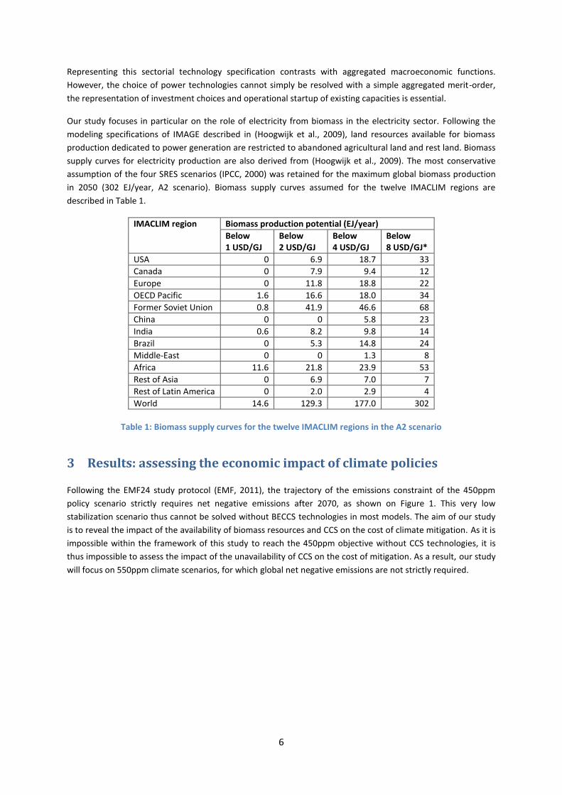
Our study focuses in particular on the role of electricity from biomass in the electricity sector. Following the

modeling specifications of IMAGE described in (Hoogwijk et al., 2009), land resources available for biomass

production dedicated to power generation are restricted to abandoned agricultural land and rest land. Biomass

supply curves for electricity production are also derived from (Hoogwijk et al., 2009). The most conservative

assumption of the four SRES scenarios (IPCC, 2000) was retained for the maximum global biomass production

in 2050 (302 EJ/year, A2 scenario). Biomass supply curves assumed for the twelve IMACLIM regions are

described in Table 1.

IMACLIM region Biomass production potential (EJ/year)

Below 1 USD/GJ

Below 2 USD/GJ

Below 4 USD/GJ

Below 8 USD/GJ*

USA 0 6.9 18.7 33

Canada 0 7.9 9.4 12

Europe 0 11.8 18.8 22

OECD Pacific 1.6 16.6 18.0 34

Former Soviet Union 0.8 41.9 46.6 68

China 0 0 5.8 23

India 0.6 8.2 9.8 14

Brazil 0 5.3 14.8 24

Middle-East 0 0 1.3 8

Africa 11.6 21.8 23.9 53

Rest of Asia 0 6.9 7.0 7

Rest of Latin America 0 2.0 2.9 4

World 14.6 129.3 177.0 302

Table 1: Biomass supply curves for the twelve IMACLIM regions in the A2 scenario

3 Results: assessing the economic impact of climate policies

Following the EMF24 study protocol (EMF, 2011), the trajectory of the emissions constraint of the 450ppm

policy scenario strictly requires net negative emissions after 2070, as shown on Figure 1. This very low

stabilization scenario thus cannot be solved without BECCS technologies in most models. The aim of our study

is to reveal the impact of the availability of biomass resources and CCS on the cost of climate mitigation. As it is

impossible within the framework of this study to reach the 450ppm objective without CCS technologies, it is

thus impossible to assess the impact of the unavailability of CCS on the cost of mitigation. As a result, our study

will focus on 550ppm climate scenarios, for which global net negative emissions are not strictly required.

7

Figure 1: Emission trajectories (450 and 550ppm scenarios)

Four technology scenarios are considered, according to the availability of the CCS technology (on or off) and

the availability of biomass resources (300 or 110 EJ/year). The scenarios are summarized in table 2.

CCS availability Biomass availability

High (300EJ/year) Low (110 EJ/year)

On (1) (2)

Off (3) (4)

Table 2 : Technology and resource scenarios

3.1 The impact of climate policies on the electricity sector

3.1.1 The electricity mix

Figures 2 and 3 show the electricity mix from 2010 to 2100 under a 550ppm climate constraint for the four

technology and resource scenarios considered.

(1)

(2)

Figure 2: Global electricity mix under two biomass resource constraints (550ppm – with CCS)

8

(3)

(4)

Figure 3: Global electricity mix under two biomass resource constraints (550ppm – no CCS)

When CCS is available, the size of biomass resources does not significantly alter the volume of electricity

production or the nature of the mix (scenarios 1 and 2 on Figure 2). Electricity production from coal and gas

without CCS is phased out by 2050 in both scenarios. The availability of biomass resources does not influence

the date of entry of the BECCS technology (2050 in the case without CCS and 2070 in the case with CCS). This

observation contrasts with optimization results under perfect foresight, for instance in (Magné et al., 2010),

where an earlier date of entry of BECCS is required in the low resource case as a way to achieve sufficient

abatement over the whole period. Our result is explained by the fact that IMACLIM is not inter-temporally

optimizing, associated with the assumption of imperfect foresight.

The availability of CCS greatly influences the nature of the electricity mix, as it locks the electricity system into a

path dominated by the use of fossil fuels (scenarios 1 and 2). The unavailability of CCS induces a wider

deployment of renewable and nuclear energy (e.g. scenario 3 compared to scenario 1). Electricity from biomass

penetrates the electricity mix earlier if CCS is unavailable (i.e. in 2050 compared to 2070 if CCS is available). This

result contrasts with those of (Luckow et al., 2010) where the absence of CCS reduces the overall biomass use.

Before 2070, the electricity mix is identical in both scenarios without CCS, but one striking result is the near

collapse of electricity production after that date in the constrained case (scenario 4).

3.1.2 CO2 tax and energy prices

This collapse of electricity production in this case can be explained by looking at the evolution of electricity

prices. Constraints are imposed on the deployment of electricity technologies. First, the renewal of production

capacities is affected by inertia. Also, the electricity module ensures that a single technology does not

dominate the supply mix. This constraint is particularly relevant in the case of nuclear power, which has raised

concerns on safety issues, and in the case of some renewable energy technologies which may fail to deploy

beyond a certain share of the electricity mix due to intermittency issues. The electricity price is thus driven by

the availability of production technologies.

9

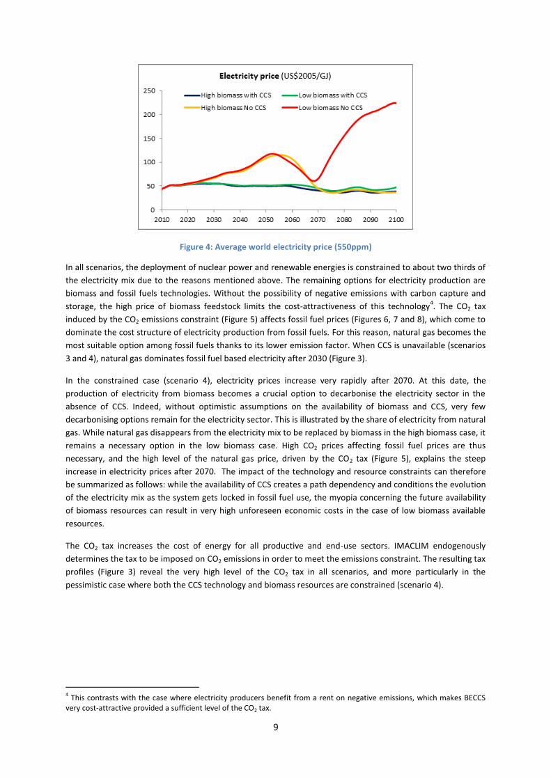
Figure 4: Average world electricity price (550ppm)

In all scenarios, the deployment of nuclear power and renewable energies is constrained to about two thirds of

the electricity mix due to the reasons mentioned above. The remaining options for electricity production are

biomass and fossil fuels technologies. Without the possibility of negative emissions with carbon capture and

storage, the high price of biomass feedstock limits the cost-attractiveness of this technology4. The CO2 tax

induced by the CO2 emissions constraint (Figure 5) affects fossil fuel prices (Figures 6, 7 and 8), which come to

dominate the cost structure of electricity production from fossil fuels. For this reason, natural gas becomes the

most suitable option among fossil fuels thanks to its lower emission factor. When CCS is unavailable (scenarios

3 and 4), natural gas dominates fossil fuel based electricity after 2030 (Figure 3).

In the constrained case (scenario 4), electricity prices increase very rapidly after 2070. At this date, the

production of electricity from biomass becomes a crucial option to decarbonise the electricity sector in the

absence of CCS. Indeed, without optimistic assumptions on the availability of biomass and CCS, very few

decarbonising options remain for the electricity sector. This is illustrated by the share of electricity from natural

gas. While natural gas disappears from the electricity mix to be replaced by biomass in the high biomass case, it

remains a necessary option in the low biomass case. High CO2 prices affecting fossil fuel prices are thus

necessary, and the high level of the natural gas price, driven by the CO2 tax (Figure 5), explains the steep

increase in electricity prices after 2070. The impact of the technology and resource constraints can therefore

be summarized as follows: while the availability of CCS creates a path dependency and conditions the evolution

of the electricity mix as the system gets locked in fossil fuel use, the myopia concerning the future availability

of biomass resources can result in very high unforeseen economic costs in the case of low biomass available

resources.

The CO2 tax increases the cost of energy for all productive and end-use sectors. IMACLIM endogenously

determines the tax to be imposed on CO2 emissions in order to meet the emissions constraint. The resulting tax

profiles (Figure 3) reveal the very high level of the CO2 tax in all scenarios, and more particularly in the

pessimistic case where both the CCS technology and biomass resources are constrained (scenario 4).

4 This contrasts with the case where electricity producers benefit from a rent on negative emissions, which makes BECCS

very cost-attractive provided a sufficient level of the CO2 tax.

10

Figure 5 : World CO2 tax to reach the 550ppm target in each technology and resource scenario

The temporary switch of the tax profiles in the high and low biomass scenarios when CCS is unavailable

(scenarios 3 and 4) between 2055 and 2070 can be explained by the profile of fossil fuel prices.

a

b

Figure 6: World oil price (550ppm)

In the case without CCS (scenarios 3 in yellow and scenario 4 in red), the oil price is higher (excl. tax, Figure 6a)

in the low biomass scenario than in the high biomass scenario until 2070. After that date, the trend is reversed.

This result may seem surprising at first, but in fact illustrates the role of fossil fuel prices in driving structural

change. The low availability of biomass imposes a constraint on the supply of biofuel, which is a substitute to

petrol. This constraint thus triggers tensions in oil markets, which are revealed by higher oil prices in scenario 4.

Higher oil prices in the short and medium term (both excluding and including the CO2 tax, cf. Figures 6a and 6b)

allow the economy to decarbonize sooner. As a result, in 2060, the structure of the economy is better suited to

achieve ambitious emission reductions in the low biomass case. In this case, the emissions constraint thus

commands a lower CO2 tax compared to the high biomass case (Figure 5, scenarios 3 and 4). However, the

situation is reversed in 2070, when electricity from biomass becomes a crucial decarbonizing option if CCS

technologies are not available. Few low-carbon options remain to fuel the expanding demand for electric

transportation, and a high CO2 tax is needed to decarbonize the transportation sector in that scenario. This

shift is also visible for tax-inclusive oil prices (Figure 6b): while the CO2 tax more than compensates the low

11

level of fossil fuel prices (excl. tax) over most of the period, this situation is briefly reversed in 2060 when the

red and yellow curves cross.

a

b

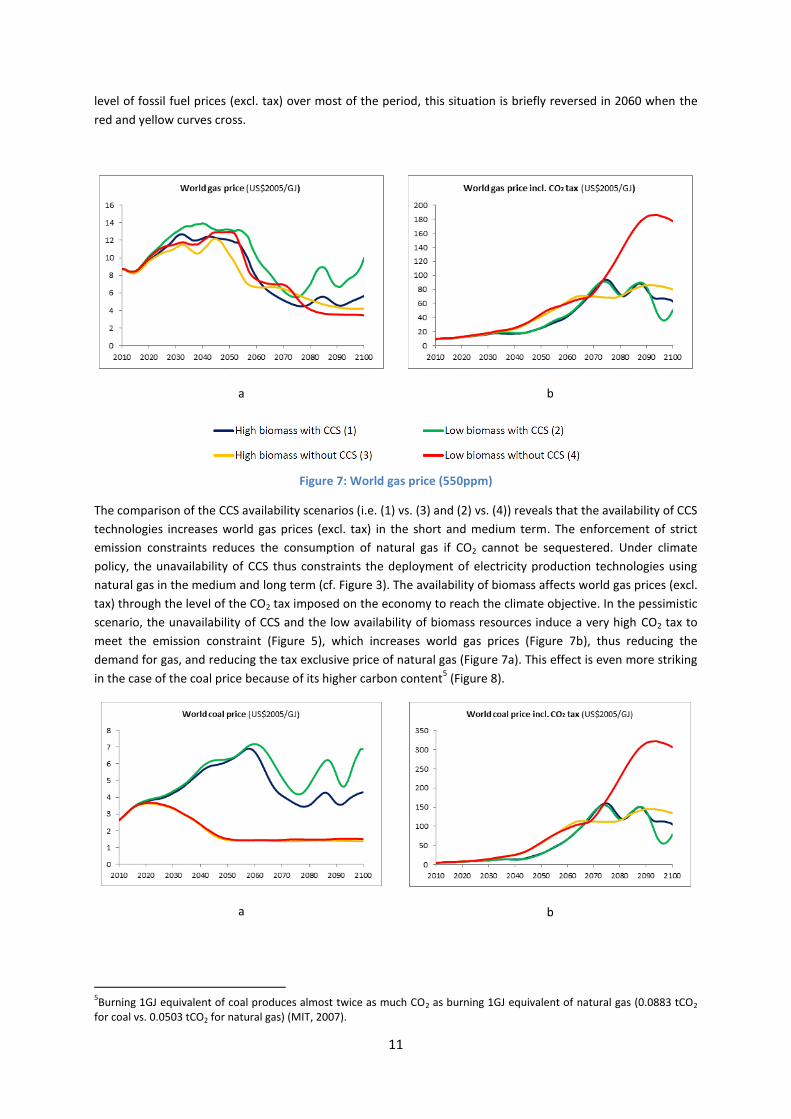
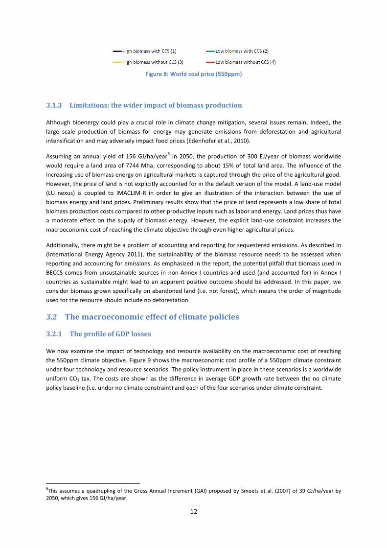
Figure 7: World gas price (550ppm)

The comparison of the CCS availability scenarios (i.e. (1) vs. (3) and (2) vs. (4)) reveals that the availability of CCS

technologies increases world gas prices (excl. tax) in the short and medium term. The enforcement of strict

emission constraints reduces the consumption of natural gas if CO2 cannot be sequestered. Under climate

policy, the unavailability of CCS thus constraints the deployment of electricity production technologies using

natural gas in the medium and long term (cf. Figure 3). The availability of biomass affects world gas prices (excl.

tax) through the level of the CO2 tax imposed on the economy to reach the climate objective. In the pessimistic

scenario, the unavailability of CCS and the low availability of biomass resources induce a very high CO2 tax to

meet the emission constraint (Figure 5), which increases world gas prices (Figure 7b), thus reducing the

demand for gas, and reducing the tax exclusive price of natural gas (Figure 7a). This effect is even more striking

in the case of the coal price because of its higher carbon content5 (Figure 8).

a

b

5Burning 1GJ equivalent of coal produces almost twice as much CO2 as burning 1GJ equivalent of natural gas (0.0883 tCO2

for coal vs. 0.0503 tCO2 for natural gas) (MIT, 2007).

12

Figure 8: World coal price (550ppm)

3.1.3 Limitations: the wider impact of biomass production

Although bioenergy could play a crucial role in climate change mitigation, several issues remain. Indeed, the

large scale production of biomass for energy may generate emissions from deforestation and agricultural

intensification and may adversely impact food prices (Edenhofer et al., 2010).

Assuming an annual yield of 156 GJ/ha/year6 in 2050, the production of 300 EJ/year of biomass worldwide

would require a land area of 7744 Mha, corresponding to about 15% of total land area. The influence of the

increasing use of biomass energy on agricultural markets is captured through the price of the agricultural good.

However, the price of land is not explicitly accounted for in the default version of the model. A land-use model

(LU nexus) is coupled to IMACLIM-R in order to give an illustration of the interaction between the use of

biomass energy and land prices. Preliminary results show that the price of land represents a low share of total

biomass production costs compared to other productive inputs such as labor and energy. Land prices thus have

a moderate effect on the supply of biomass energy. However, the explicit land-use constraint increases the

macroeconomic cost of reaching the climate objective through even higher agricultural prices.

Additionally, there might be a problem of accounting and reporting for sequestered emissions. As described in

(International Energy Agency 2011), the sustainability of the biomass resource needs to be assessed when

reporting and accounting for emissions. As emphasized in the report, the potential pitfall that biomass used in

BECCS comes from unsustainable sources in non-Annex I countries and used (and accounted for) in Annex I

countries as sustainable might lead to an apparent positive outcome should be addressed. In this paper, we

consider biomass grown specifically on abandoned land (i.e. not forest), which means the order of magnitude

used for the resource should include no deforestation.

3.2 The macroeconomic effect of climate policies

3.2.1 The profile of GDP losses

We now examine the impact of technology and resource availability on the macroeconomic cost of reaching

the 550ppm climate objective. Figure 9 shows the macroeconomic cost profile of a 550ppm climate constraint

under four technology and resource scenarios. The policy instrument in place in these scenarios is a worldwide

uniform CO2 tax. The costs are shown as the difference in average GDP growth rate between the no climate

policy baseline (i.e. under no climate constraint) and each of the four scenarios under climate constraint.

6This assumes a quadrupling of the Gross Annual Increment (GAI) proposed by Smeets et al. (2007) of 39 GJ/ha/year by

2050, which gives 156 GJ/ha/year.

13

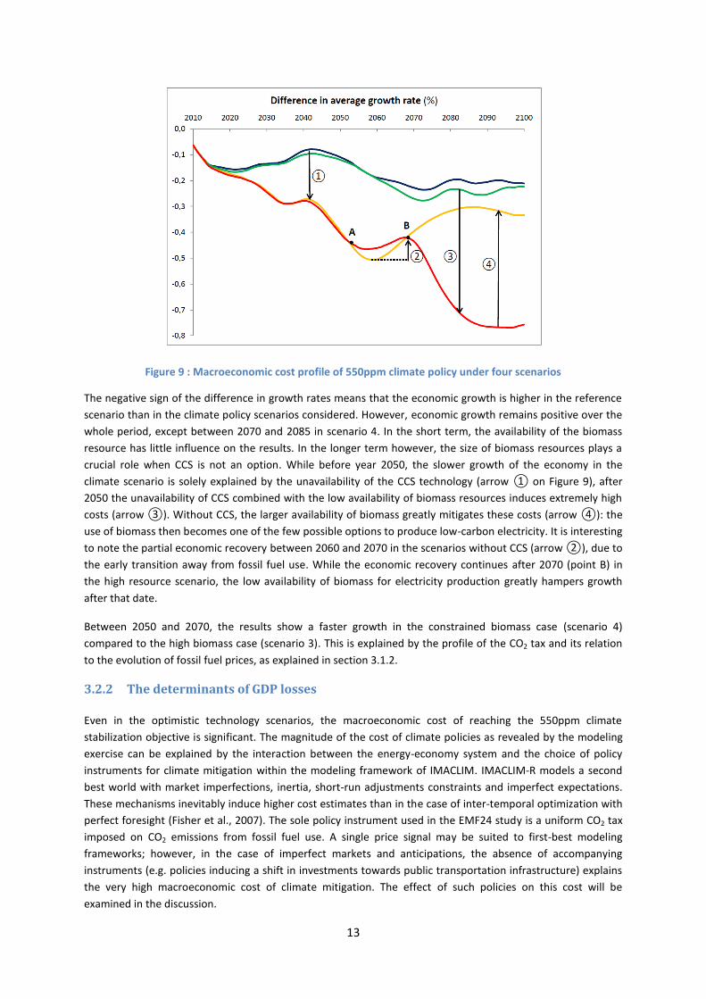
Figure 9 : Macroeconomic cost profile of 550ppm climate policy under four scenarios

The negative sign of the difference in growth rates means that the economic growth is higher in the reference

scenario than in the climate policy scenarios considered. However, economic growth remains positive over the

whole period, except between 2070 and 2085 in scenario 4. In the short term, the availability of the biomass

resource has little influence on the results. In the longer term however, the size of biomass resources plays a

crucial role when CCS is not an option. While before year 2050, the slower growth of the economy in the

climate scenario is solely explained by the unavailability of the CCS technology (arrow ① on Figure 9), after

2050 the unavailability of CCS combined with the low availability of biomass resources induces extremely high

costs (arrow ③). Without CCS, the larger availability of biomass greatly mitigates these costs (arrow ④): the

use of biomass then becomes one of the few possible options to produce low-carbon electricity. It is interesting

to note the partial economic recovery between 2060 and 2070 in the scenarios without CCS (arrow ②), due to

the early transition away from fossil fuel use. While the economic recovery continues after 2070 (point B) in

the high resource scenario, the low availability of biomass for electricity production greatly hampers growth

after that date.

Between 2050 and 2070, the results show a faster growth in the constrained biomass case (scenario 4)

compared to the high biomass case (scenario 3). This is explained by the profile of the CO2 tax and its relation

to the evolution of fossil fuel prices, as explained in section 3.1.2.

3.2.2 The determinants of GDP losses

Even in the optimistic technology scenarios, the macroeconomic cost of reaching the 550ppm climate

stabilization objective is significant. The magnitude of the cost of climate policies as revealed by the modeling

exercise can be explained by the interaction between the energy-economy system and the choice of policy

instruments for climate mitigation within the modeling framework of IMACLIM. IMACLIM-R models a second

best world with market imperfections, inertia, short-run adjustments constraints and imperfect expectations.

These mechanisms inevitably induce higher cost estimates than in the case of inter-temporal optimization with

perfect foresight (Fisher et al., 2007). The sole policy instrument used in the EMF24 study is a uniform CO2 tax

imposed on CO2 emissions from fossil fuel use. A single price signal may be suited to first-best modeling

frameworks; however, in the case of imperfect markets and anticipations, the absence of accompanying

instruments (e.g. policies inducing a shift in investments towards public transportation infrastructure) explains

the very high macroeconomic cost of climate mitigation. The effect of such policies on this cost will be

examined in the discussion.

14

Here, we have a closer look at the influence of two major indicators of economic activity on economic growth:

industrial production costs and consumer prices. The level of the CO2 tax has a direct economic effect on all

sectors. We propose here to focus on its impact on the industrial sector and on households in the optimistic

technology case (scenario 1).

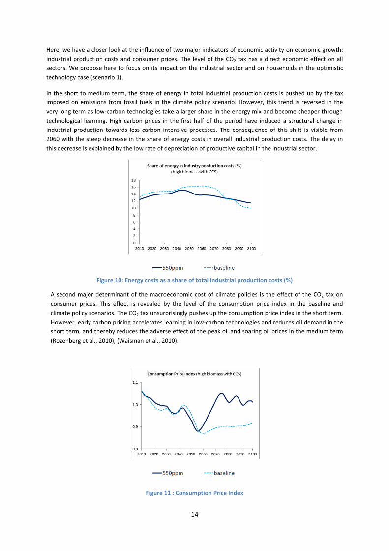
In the short to medium term, the share of energy in total industrial production costs is pushed up by the tax

imposed on emissions from fossil fuels in the climate policy scenario. However, this trend is reversed in the

very long term as low-carbon technologies take a larger share in the energy mix and become cheaper through

technological learning. High carbon prices in the first half of the period have induced a structural change in

industrial production towards less carbon intensive processes. The consequence of this shift is visible from

2060 with the steep decrease in the share of energy costs in overall industrial production costs. The delay in

this decrease is explained by the low rate of depreciation of productive capital in the industrial sector.

Figure 10: Energy costs as a share of total industrial production costs (%)

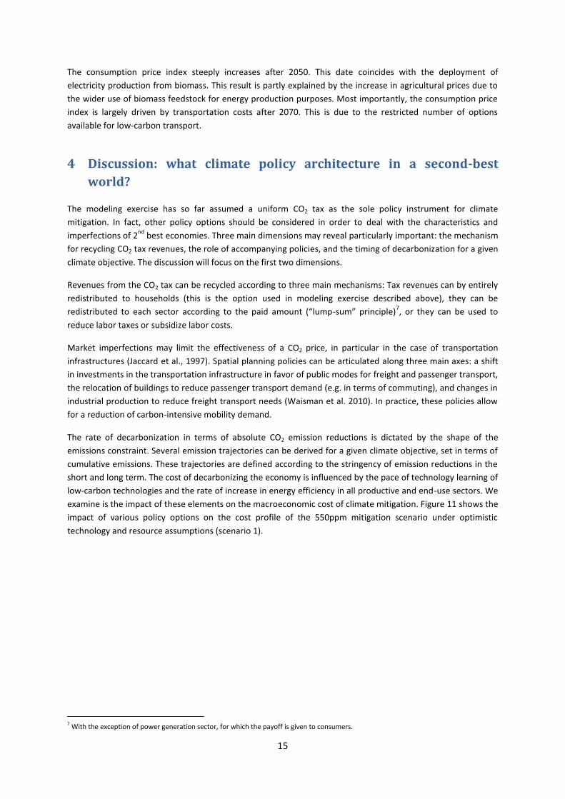
A second major determinant of the macroeconomic cost of climate policies is the effect of the CO2 tax on

consumer prices. This effect is revealed by the level of the consumption price index in the baseline and

climate policy scenarios. The CO2 tax unsurprisingly pushes up the consumption price index in the short term.

However, early carbon pricing accelerates learning in low-carbon technologies and reduces oil demand in the

short term, and thereby reduces the adverse effect of the peak oil and soaring oil prices in the medium term

(Rozenberg et al., 2010), (Waisman et al., 2010).

Figure 11 : Consumption Price Index

15

The consumption price index steeply increases after 2050. This date coincides with the deployment of

electricity production from biomass. This result is partly explained by the increase in agricultural prices due to

the wider use of biomass feedstock for energy production purposes. Most importantly, the consumption price

index is largely driven by transportation costs after 2070. This is due to the restricted number of options

available for low-carbon transport.

4 Discussion: what climate policy architecture in a second-best

world?

The modeling exercise has so far assumed a uniform CO2 tax as the sole policy instrument for climate

mitigation. In fact, other policy options should be considered in order to deal with the characteristics and

imperfections of 2nd

best economies. Three main dimensions may reveal particularly important: the mechanism

for recycling CO2 tax revenues, the role of accompanying policies, and the timing of decarbonization for a given

climate objective. The discussion will focus on the first two dimensions.

Revenues from the CO2 tax can be recycled according to three main mechanisms: Tax revenues can by entirely

redistributed to households (this is the option used in modeling exercise described above), they can be

redistributed to each sector according to the paid amount (“lump-sum” principle)7, or they can be used to

reduce labor taxes or subsidize labor costs.

Market imperfections may limit the effectiveness of a CO2 price, in particular in the case of transportation

infrastructures (Jaccard et al., 1997). Spatial planning policies can be articulated along three main axes: a shift

in investments in the transportation infrastructure in favor of public modes for freight and passenger transport,

the relocation of buildings to reduce passenger transport demand (e.g. in terms of commuting), and changes in

industrial production to reduce freight transport needs (Waisman et al. 2010). In practice, these policies allow

for a reduction of carbon-intensive mobility demand.

The rate of decarbonization in terms of absolute CO2 emission reductions is dictated by the shape of the

emissions constraint. Several emission trajectories can be derived for a given climate objective, set in terms of

cumulative emissions. These trajectories are defined according to the stringency of emission reductions in the

short and long term. The cost of decarbonizing the economy is influenced by the pace of technology learning of

low-carbon technologies and the rate of increase in energy efficiency in all productive and end-use sectors. We

examine is the impact of these elements on the macroeconomic cost of climate mitigation. Figure 11 shows the

impact of various policy options on the cost profile of the 550ppm mitigation scenario under optimistic

technology and resource assumptions (scenario 1).

7 With the exception of power generation sector, for which the payoff is given to consumers.

16

Figure 11: Cost with and without accompanying policies - (550ppm, optimistic technology case)

Carbon tax revenues are used to decrease labor taxes. This tax recycling option reduces the short and medium

term costs of reaching the climate objective, as demonstrated by the comparison in Figure 11 between the

“reference” climate scenario (blue) and the “efficient tax recycling” scenario (pink). As was seen earlier, short

term economic losses with a single CO2 tax are mainly explained by the increase in production costs, for

instance in the industrial sector. The decrease in labor taxes reduces labor costs and overall production costs in

all sectors, thus reducing economic losses compared to the reference scenario,

Accompanying infrastructure policies (labeled “Infrastructure policies” in Figure 11) aimed at reducing mobility

demand significantly reduce the overall macroeconomic costs of reaching the climate objective. Their effect is

particularly visible in the medium and long term. In the medium term (2030-2050), new infrastructures start

reducing oil demand, thus delaying the peak oil. The associated increase in oil prices and its adverse effect on

growth is partly avoided, and infrastructure policies even induce some net benefits compared to the baseline

scenario without any CO2 constraint. In the long term (after 2070), the high level of the CO2 tax in the reference

scenario follows the need to decarbonize the transportation sector. Some low carbon options are available,

namely biofuels and electric vehicles, but the cost of their deployment highly depends on the pace of technical

change in this sector (Waisman et al., 2010). The role of infrastructure policies in reducing mobility demand is

thus crucial at that time horizon, as shown by the comparison of the trends in the difference in the average

growth rate between the reference and “infrastructure policies” scenarios: infrastructure policies allow for a

partial catch-up with the no constraint baseline scenario after 2070. The combination of these policies and the

use of CO2 tax revenues to reduce labor taxes allows for net economic benefits of climate policies in the

medium term.

5 Conclusion

The modeling exercise has revealed the sometimes complex dynamics of the links between electricity

production and prices, fossil fuel markets and demand for energy at various time horizons. The availability of

carbon capture and storage creates a path dependency and conditions the evolution of the electricity mix and

the low availability of biomass resources can result in very high unforeseen economic costs. CCS technologies

are beneficial to the economy in the short to medium term, when fossil fuel resources remain available and

relatively cheap. However, in the longer term, economies are locked in an electricity mix that is greatly

17

dependent on the use of fossil fuels. The unavailability of CCS combined with the low availability of biomass

resources induces extremely high costs in the long term. Without CCS, the use of biomass then becomes one of

the few remaining options to produce low-carbon electricity, making biomass a robust technology option.

The macroeconomic cost of climate mitigation is in part driven by the increase in production costs in all sectors

and the increase in consumer prices, due to higher fossil fuel prices. The study revealed that additional policy

options should be implemented to achieve ambitious climate objectives. In particular, the combination of

recycling tax revenues to reduce labor taxes and the implementation of infrastructure policies may induce net

economic benefits.

6 References

Arango, S., Larsen, E., 2011. Cycles in deregulated electricity markets: Empirical evidence from two decades. Energy Policy 39 (5) 2457-2466. Atkeson, A., Kehoe, P.J., 1999. Models of Energy Use: Putty-Putty versus Putty-Clay. The American Economic Review 89 (4) 1028-1043. Azar, C., Lindgren, K., Larson, E., Möllersten, K., 2006. Carbon Capture and Storage from fossil fuels and

biomass – Costs and potential role in stabilizing the atmosphere. Climatic Change 74 47-79.

Berndt E.R., Wood, D.O., 1975. Technology, prices, and the derived demand for energy. The Review of

Economics and Statistics 57 (3) 259-268.

Bhattacharyya, S. C., 1996. Applied general equilibrium models for energy studies: a survey. Energy Economics

18 (3) 145-164.

Bunn, D.W., Larsen, E.R.,. 1992. Sensitivity of reserve margin to factors influencing investment behaviour in the

electricity market of England and Wales. Energy Policy 20 (5) 420-429.

Crassous, R., Hourcade, J.-C., Sassi, O., 2006. Endogenous structural change and climate targets: modeling

experiments with Imaclim-R. The Energy Journal, Special Issue on the Innovation Modeling Comparison Project.

Downing, T.E., Anthoff, D., Butterfield, R., Ceronsky, M., Grubb,M., Guo, J., Hepburn, C., Hope, C., Hunt, A., Li,

A., Markandya, A., Moss, S., Nyong, A., Tol, R.S.J., Watkiss, P., 2005. Social Cost of Carbon: A Closer Look at

Uncertainty. Final project report. Available at: http://www.decc.gov.uk

Edenhofer, O., Knopf, B., Barker, T., Baumstark, L., Bellevrat, E., Château, B., Criqui, P., Isaac, M., Kitous, A.,

Kypreos, S., Leimbach, M., Lessmann, K., Magné, B., Scrieciu, S., Turton, H., van Vuuren, D.P., 2010. The

Economics of Low Stabilization: Model Comparison of Mitigation Strategies and Costs. The Energy Journal 31

(Special Issue 1) 11-48.

Energy Modeling Forum (EMF), 2011. EMF 24: Technology Strategies for Achieving Climate Policy Objectives.

Available at: http://emf.stanford.edu/research/emf24/

Finn, M. G., 2000. Perfect competition and the effects of energy price increases on economic activity. Journal of

Money, Credit and Banking: 400-416.

Fisher, B.S., Nakicenovic, N., Alfsen, K., Corfee Morlot, J., de la Chesnaye, F., Hourcade, J.-C., Jiang,, K., Kainuma,

M., La Rovere, E., Matysek, A., Rana, A., Riahi, K., Richels, R., Rose, S., van Vuuren, D., Warren, R., 2007. Issues

related to mitigation in the long term context, In Climate Change 2007: Mitigation. Contribution of Working

18

Group III to the Fourth Assessment Report of the Inter-governmental Panel on Climate Change, B. Metz, O.R.

Davidson, P.R. Bosch, R. Dave, L.A. Meyer (eds), Cambridge University Press, Cambridge, UK.

Ford, A., 1999. Cycles in competitive electricity markets: a simulation study of the western United States.

Energy Policy 27 (11) 637-658.

Frondel, M., Schmidt, C., 2002. The Capital-Energy Controversy: an artifact of cost shares? The Energy Journal

23 (3) 53-80.

Ghersi, F., Hourcade, J.-C., 2006. Macroeconomic Consistency Issues in E3 Modeling: The Continued Fable of

the Elephant and the Rabbit. The Energy Journal Special issue on Hybrid Modeling of Energy Environment

Policies: reconciling Bottom-up and Top-down 39-62.

Hoogwijk, M., Faaij, A., de Vries, B., Turkenburg, W., 2009. Exploration of regional and global cost-supply curves

of biomass energy from short-rotation crops at abandoned cropland and rest land under four IPCC SRES land-

use scenarios. Biomass and Bioenergy 33: 26-43.

Hourcade J.-C., 1993. Modelling long-run scenarios: Methodology lessons from a prospective study on a low

CO2 intensive country. Energy Policy 21 (3) 309-326.

Intergovernmental Panel on Climate Change (IPCC), 2005. Special Report on Carbon Dioxide Capture and

Storage. Prepared by Working Group III of the Intergovernmental Panel on Climate Change. Metz, B., O.

Davidson, H. C. de Coninck, M. Loos, and L. A. Meyer (eds.). Cambridge University Press, Cambridge, United

Kingdom and New York, NY, USA.

Intergovernmental Panel on Climate Change (IPCC), 2000. Special Report on Emissions Scenarios. Cambridge

University Press, Cambridge, UK.

International Energy Agency, 2011. Combining Bioenergy with CCS - Reporting and Accounting for Negative Emissions under UNFCCC and the Kyoto Protocol, International Energy Agency. Available at: http://www.iea.org/publications/free_new_Desc.asp?PUBS_ID=2487 Jaccard, M., Failing, L., Berry, T., 1997. From equipment to infrastructure: community energy management and greenhouse gas emission reduction. Energy Policy. 25 (13) 1065-1074. Jorgenson, D.W., Fraumeni, B.M., 1981. Relative prices and technical change. Modeling and Measuring Natural Resource Substitution 17-47. Luckow, P., Dooley, J.J., Wise, M.A., Kim, S.H., 2010. Large-scale utilization of biomass energy and carbon

dioxide capture and storage in the transport and electricity sectors under stringent CO2 concentration limit

scenarios. International Journal of Greenhouse Gas Control 4 (5) 865-877

Magné, B., Kypreos, S., Turton, H., 2010, Technology Options for Low Stabilization Pathways with MERGE. The

Energy Journal 31 (Special Issue 1) 83-108.

McFarland, J.R., Reilly, J.M., Herzog, H.J., 2004. Representing energy technologies in top-down economic

models using bottom-up information. Energy Economics 26 (4) 685-707.

MIT, 2007. Units and Conversions Fact Sheet. Produced by Derek Supple, MIT Energy Club. Available at

http://web.mit.edu/mit_energy

Olsina, F., Garcés, F., Haubrich, H.-J., 2006. Modeling long-term dynamics of electricity markets. Energy Policy

34 1411–1433.

19

Rostow, W., 1993. Nonlinear Dynamics and Economics: A Historian’s Perspective. In: Nonlinear Dynamics and

Evolutionary Economics. Eds. Richard H. Day, Ping Chen. Oxford: Oxford: 14-17.

Rotemberg, J., Woodford, M., 1996. Imperfect Competition and the Effects of Energy Price Increases on

Economic Activity. Journal of Money, Credit and Banking 28 (4) 549-577.

Rozenberg, J., Hallegatte, S., Vogt-Schilb, A., Sassi, O., Guivarch, C., Waisman, H., Hourcade, J.-C., 2010. Climate

policies as a hedge against the uncertainty on future oil supply, Climatic Change Letters

Sassi O., Crassous R., Hourcade J.-C., Gitz V., Waisman H., Guivarch C., 2010. Imaclim-R: a modelling framework

to simulate sustainable development pathways. International Journal of Global Environmental Issues 10: 5-24.

Silk, J.I., Joutz, F.L., 1997. Short and long-run elasticities in US residential electricity demand: a co-integration

approach. Energy Economics 19 (4) 493-513.

Smeets, E., Faaij, A., Lewandowski, I., Turkenburg, W., 2007. A bottom-up assessment and review of global bio-

energy potentials to 2050. Progress in Energy and Combustion Science 33 (1) 56-106

Solow, R.M., 1956. A Contribution to the Theory of Economic Growth. The Quarterly Journal of Economics 70

(1) 65-94.

Sterman, J.D., 2000. Business Dynamics: Systems Thinking and Modeling for a Complex World. Irwin/McGraw-

Hill.

Taylor, L.D., 1975. The demand for electricity: a survey. The Bell Journal of Economics 74-110.

The Royal Society, 2009. Geoengineering the Climate: science, governance and uncertainty. Report 10/09.

van Vuuren, D.P., Bellevrat, E., Kitous, A., Isaac, M., 2010. Bio-energy use and low stabilization scenarios. The

Energy Journal 31 (Special Issue 1) 192-222.

Waisman, H., Guivarch, C., Grazi, F., Hourcade, J.-C., 2010. The IMACLIM-R Model: Infrastructures, Technical

Inertia and the Costs of Low Carbon Futures under Imperfect Foresight . Climatic Change, in press.

Wise, M., Calvin, K., Thomson, A., Clarke, L., Bond-Lamberty, B., Sands, R., Smith, S.J., Janetos, A., Edmonds, J.,

2009. Implications of limiting CO2 concentrations for land use and energy. Science 324 (5931) 1183-1186.