Needs For Alternatives To GAC/MH I
320
Needs For and Alternatives To GAC/MH I‐001a November 2013 Page 1 of 1 REFERENCE: Appendix 7.4 Capacity Value of Wind Resources; 1 2 PREAMBLE: Appendix 7.2 states "For the purpose of high‐level screening, levelized 3 costs for new generation were obtained from the U.S. Energy Information 4 Administration (EIA) 2013 Annual Energy Outlook Early Release." and 5 Table 7.2.2 specifies a Levelized Cost without Transmission for 100 MW On‐Shore Wind 6 Project Low Capital Cost Case of $62/MW.h and High Capital Cost Case of $99/MW.h. 7 8 QUESTION: 9 Please provide a copy of the U.S. Energy Information Administration 2013 Annual Energy 10 Outlook Early Release and cite where these levelized cost estimates are provided in this report. 11 12 RESPONSE: 13 The portion of EIA 2013 Early Release that contains levelized cost information is available at 14 http://www.eia.gov/forecasts/aeo/er/electricity_generation.cfm. As stated in Appendix 7.2, 15 page 5, Figure Appendix 7.2‐1 provides the levelized cost ranges for resource technologies as 16 provided in the EIA Annual Energy Outlook 2013. 17 18 Levelized cost information for generic on‐shore wind resource options contained in Table 7.2‐2 19 from Appendix 7.2 reflect levelized costs based on potential development of resource 20 technologies in Manitoba and were not derived from the EIA 2013 Early Release information. 21 The levelized cost estimates provided in Table 7.2‐2 for a 100 MW on‐shore wind project built 22 in Manitoba, are cited in Appendix 7.2, page 326. 23 24 Please also refer to Manitoba Hydro’s responses to GAC/MH I‐001b and GAC/MH I‐001c. 25
Transcript of Needs For Alternatives To GAC/MH I

Needs For and Alternatives To GAC/MH I‐001a
November 2013 Page 1 of 1
REFERENCE: Appendix 7.4 Capacity Value of Wind Resources; 1
2
PREAMBLE: Appendix 7.2 states "For the purpose of high‐level screening, levelized 3
costs for new generation were obtained from the U.S. Energy Information 4
Administration (EIA) 2013 Annual Energy Outlook Early Release." and 5
Table 7.2.2 specifies a Levelized Cost without Transmission for 100 MW On‐Shore Wind 6
Project Low Capital Cost Case of $62/MW.h and High Capital Cost Case of $99/MW.h. 7
8
QUESTION: 9
Please provide a copy of the U.S. Energy Information Administration 2013 Annual Energy 10
Outlook Early Release and cite where these levelized cost estimates are provided in this report. 11
12
RESPONSE: 13
The portion of EIA 2013 Early Release that contains levelized cost information is available at 14
http://www.eia.gov/forecasts/aeo/er/electricity_generation.cfm. As stated in Appendix 7.2, 15
page 5, Figure Appendix 7.2‐1 provides the levelized cost ranges for resource technologies as 16
provided in the EIA Annual Energy Outlook 2013. 17
18
Levelized cost information for generic on‐shore wind resource options contained in Table 7.2‐2 19
from Appendix 7.2 reflect levelized costs based on potential development of resource 20
technologies in Manitoba and were not derived from the EIA 2013 Early Release information. 21
The levelized cost estimates provided in Table 7.2‐2 for a 100 MW on‐shore wind project built 22
in Manitoba, are cited in Appendix 7.2, page 326. 23
24
Please also refer to Manitoba Hydro’s responses to GAC/MH I‐001b and GAC/MH I‐001c.25

Needs For and Alternatives To GAC/MH I‐001b
November 2013 Page 1 of 1
REFERENCE: Appendix 7.4 Capacity Value of Wind Resources 1
2
QUESTION: 3
If these levelized cost estimates are not specified in this report, please provide the workpapers 4
that were used to derive these estimates. 5
6
RESPONSE: 7
The source documents and papers used to derive the levelized cost estimates for a wind project 8
built in Manitoba are considered confidential information. 9
10
For additional information regarding levelized costs of wind projects built in Manitoba please 11
see Manitoba Hydro’s response to GAC/MH I‐001c. 12

Needs For and Alternatives To GAC/MH I‐001c
November 2013 Page 1 of 1
REFERENCE: Appendix 7.4 Capacity Value of Wind Resources 1
2
QUESTION: 3
What would be the Levelized Cost for the Reference Capital Cost Case for 100 MW On‐Shore 4
Wind Project? 5
6
RESPONSE: 7
The levelized cost for a 100 MW on‐shore wind project at the reference capital cost of 8
$2100/kW without transmission is $75/MWh. 9
10
As identified in Manitoba Hydro’s letter to the Public Utilities Board on September 13, 2013 and 11
posted on Manitoba Hydro’s external website, after the submission of the NFAT filing it was 12
identified that the capital cost for the wind resource option used throughout the filing was 13
approximately 5% higher than it should have been. The restated capital costs of wind 14
generation normalized per kW and reported as Overnight Capital Costs ($/kW) in Appendix 7.2 15
are as follows: 16
High Case ‐ $2800/kW 17
Reference Case ‐ $2100/kW 18
Low Case ‐ $1500/kW19

Needs For and Alternatives To GAC/MH I‐002
November 2013 Page 1 of 1
REFERENCE: Appendix 7.2 Range of Resource Options; Section: 1.2; Page No.: 9 of 42 1
2
PREAMBLE: Table 7.2.2 specifies a Levelized Cost without Transmission for 65 MW On‐3
Shore Wind Project of $78/MW.h relative to the Low and High Capital Cost Case 4
Levelized Cost Estimates of $62/MW.h and $99/MW.h. For 100 MW On‐Shore Wind 5
Project 6
7
QUESTION: 8
Do the Levelized Cost estimates consider the economies of scale associated with building a 65 9
MW wind project rather than a 100 MW wind project? Please explain the basis for any 10
assumptions and provide all work papers used to derive any economies of scale adjustment. 11
12
RESPONSE: 13
As stated on page 33 of Chapter 7 of the NFAT Business Case, a generic 65 MW wind project 14
was used for future assessments and evaluations In the NFAT Business Case, the generic cost 15
for a wind project was based on a range of costs experienced for recent wind projects with 16
varying capacities (50 WM to 200 MW) aggregated to represent a 100 MW project. The cost for 17
the 65 MW wind project was scaled from the 100 MW project and therefore the benefit from 18
any economics of scale of the larger project are embedded in the cost for the 65MW wind 19
project. 20
21

Needs For and Alternatives To GAC/MH I‐003a
November 2013 Page 1 of 2
REFERENCE: Appendix 9.3 Economic Evaluation Documentation; Section: 2.1.3; Page 1
No.: p. 37 2
3
PREAMBLE: "Table 2.5 Contrasts the Percentage Difference of Low and High Capital 4
Costs Relative to Reference Capital Costs for the Resource Alternatives. The low end 5
percentage for hydro projects is ‐8.8% (Conawapa) versus ‐26.2% for wind and high end 6
13.2% (Keeyask) for hydro versus 7
8
QUESTION: 9
How do these percentage differences account for the fact that a considerably greater 10
percentage of the total project costs for the gas‐fired and wind technologies are for what are 11
effectively modular components which can be assembled in a factory and for which costs are 12
more readily known? 13
14
RESPONSE: 15
The range of capital costs for wind and natural gas‐fired projects included in the analysis is 16
primarily related to the level of estimate as defined by the AACE Cost Classification System. 17
Under AACE, the level of capital cost estimate for wind and natural gas‐fired projects used in 18
the NFAT Business Case is a Class 5 estimate which has a higher uncertainty due to the lesser 19
amount of overall engineering completion at this time when compared to that of the Keeyask 20
and Conawapa generating stations. Conawapa is a Class 3 estimate and Keeyask is between a 21
Class 2 and Class 3 estimate, as stated in Appendix 2.4. 22
23
The modular characteristics of gas‐fired and wind generation technologies have been taken into 24
consideration in establishing the range for the capital cost estimate. As shown in Appendix 9.3, 25
Table 2.3 AACE Cost Estimate Classification Table the expected accuracy range for Class 5 26
estimates can vary from ‐20% to ‐50% for the low end of the range and from +30% to +100% 27
for the high end of the range. The cost estimate ranges for wind and natural gas‐fired resources 28
fall within a narrower expected accuracy range than the outer bounds of the Class 5 estimate, 29

Needs For and Alternatives To GAC/MH I‐003a
November 2013 Page 2 of 2
primarily due to the modular characteristics of these technologies, the low level of complexity 1
in completing the project, and the maturity of the technologies. These ranges were based on 2
systemic risks as calculated by a third party risk and contingency consultant and are consistent 3
with and developed using AACE Recommended Practice 18r‐97. 4

Needs For and Alternatives To GAC/MH I‐003b
November 2013 Page 1 of 1
REFERENCE: Appendix 9.3 Economic Evaluation Documentation; Section: 2.1.3; Page 1
No.: p. 37 2
3
PREAMBLE: "Table 2.5 Contrasts the Percentage Difference of Low and High Capital 4
Costs Relative to Reference Capital Costs for the Resource Alternatives. The low end 5
percentage for hydro projects is ‐8.8% (Conawapa) versus ‐26.2% for wind and high end 6
13.2% (Keeyask) 7
8
QUESTION: 9
Please confirm that Manitoba Hydro believes that there are greater capital cost escalation risks 10
when expressed in terms of the percentage difference relative to the reference capital costs for 11
a wind and a gas turbine project (SCGT or CCGT) than for the two proposed hydro projects. 12
13
RESPONSE: 14
Not confirmed. 15
16
The range in the estimates is based on a number of factors such as extent of project planning, 17
extent of detailed engineering design available to define project scope, estimate inclusiveness, 18
estimating data quality, percent fixed price, maturity of technology, facility complexity and 19
project complexity. 20
21
Please see Manitoba Hydro’s response to GAC/MH I‐003a, which provides a description of the 22
AACE Cost Classification System applied in the preparation of the capital cost estimates for the 23
NFAT Business Cases. 24

Needs For and Alternatives To GAC/MH I‐004a
November 2013 Page 1 of 2
REFERENCE: Chapter 7: Screening of Manitoba Resource Options; Section: 7.2.4; Page 1
No.: p. 32 2
3
PREAMBLE: Chapter 7 of NFAT Business Case Summary notes that "industry forecasts 4
to 2030 anticipate a 45% increase in energy output from wind turbines, assuming that 5
material costs decrease by 10% in real terms from current levels." 6
7
QUESTION: 8
Please indicate how the capital cost expressed in $/kW or wind project output assumptions 9
(e.g., capacity factor) used in the NFAT analysis consider such increases in output or decreases 10
in material costs. 11
12
RESPONSE: 13
In the NFAT Business Case, reference capital costs were based on current costs for wind 14
generation with no escalation going forward. Energy output for wind generation resources was 15
based on a 40% capacity factor. 16
17
The 40% capacity factor assumed in the analysis is consistent with recent experience for wind 18
generation resources in Manitoba having 80 metre hub heights. Forecasted increases in energy 19
output from wind turbines are to a large degree dependent on having larger turbines and/or 20
having higher hub heights (higher towers) accessing higher wind speeds. However, there is 21
uncertainty as to whether such improvements will materialize. Should such benefits materialize 22
any resulting increase in energy output would have to offset higher costs associated with larger 23
turbines and tower construction. 24
25
Key factors driving Manitoba Hydro’s assumption to use current wind generation costs for the 26
reference capital cost and a 40% capacity factor include uncertainty in infrastructure costs 27

Needs For and Alternatives To GAC/MH I‐004a
November 2013 Page 2 of 2
related to higher towers, technical challenges with erecting higher towers, and uncertainty in 1
commodity prices. 2
Needs For and Alternatives To GAC/MH I‐004b
November 2013 Page 1 of 1
REFERENCE: Chapter 7: Screening of Manitoba Resource Options; Section: 7.2.4; Page 1
No.: p. 32 2
3
PREAMBLE: Chapter 7 of NFAT Business Case Summary notes that "industry forecasts 4
to 2030 anticipate a 45% increase in energy output from wind turbines, assuming that 5
material costs decrease by 10% in real terms from current levels." 6
7
QUESTION: 8
What assumptions were made regarding how the capital costs of wind projects expressed in 9
$/kW would change over time, indicating the percentage change or the $/kW cost and the year 10
for which such costs apply. 11
12
RESPONSE: 13
Please see Manitoba Hydro’s response to GAC/MH I‐004a. 14

Needs For and Alternatives To GAC/MH I‐004c
November 2013 Page 1 of 1
REFERENCE: Chapter 7: Screening of Manitoba Resource Options; Section: 7.2.4; Page 1
No.: p. 32 2
3
PREAMBLE: Chapter 7 of NFAT Business Case Summary notes that "industry forecasts 4
to 2030 anticipate a 45% increase in energy output from wind turbines, assuming that 5
material costs decrease by 10% in real terms from current levels." 6
7
QUESTION: 8
What assumptions were made regarding how the energy output and resulting capacity factors 9
of wind projects would change over time? 10
11
RESPONSE: 12
Please Manitoba Hydro’s response to GAC/MH I‐004a. 13

Needs For and Alternatives To GAC/MH I‐004d
November 2013 Page 1 of 1
REFERENCE: Chapter 7: Screening of Manitoba Resource Options; Section: 7.2.4; Page 1
No.: p. 32 2
3
PREAMBLE: Chapter 7 of NFAT Business Case Summary notes that "industry forecasts 4
to 2030 anticipate a 45% increase in energy output from wind turbines, assuming that 5
material costs decrease by 10% in real terms from current levels." 6
7
QUESTION: 8
What assumptions were made regarding how the energy output and resulting capacity factors 9
of wind projects would change over time? 10
11
RESPONSE: 12
Please see Manitoba Hydro’s response to GAC/MH I‐004a. 13

Needs For and Alternatives To GAC/MH I‐005
November2013 Page 1 of 1
REFERENCE: Appendix 7.1 Emerging Energy Technology Review; Section: 4.1.2; Page 1
No.: 20 2
3
PREAMBLE: An International Energy Agency (IEA) analysis projects a cost reduction in 4
LCOE of about 20 to 30% by 2030 (based on $2011). 5
6
QUESTION: 7
Please indicate how the LCOE for wind used in the analysis considers such cost reductions. 8
9
RESPONSE: 10
Please see Manitoba Hydro’s response to GAC/MH I‐004a. 11

Needs For and Alternatives To GAC/MH I‐006
November 2013 Page 1 of 1
REFERENCE: Appendix 7.2 Range of Resource Options; Section: 1.2; Page No.: 9 1
2
PREAMBLE: Table 7.2.2 specifies a 40% lifetime capacity factor for on‐shore wind. 3
4
QUESTION: 5
Please provide the work papers and assumptions that were used to derive this 40% capacity 6
factor value. 7
8
RESPONSE: 9
The 40% lifetime capacity factor assumption for on‐shore wind in Manitoba was derived from 10
actual experience from the two wind farms in Manitoba. Manitoba Hydro’s 2012/13 Annual 11
Report at page 101 states wind purchases of 0.9 billion kWh. Based on installed capacities of St. 12
Leon at 120.5 MW and St. Joseph at 138 MW, the calculation results in a capacity factor (CF) of 13
39.72% (40% rounded up) for purchased wind energy. 14
15
Capacity Factor = (900,000,000 kW.h/year/ (258,500 kW x 24 hours/day x 365.25 days/year)) x 16
100% = 39.72% 17

Needs For and Alternatives To GAC/MH I‐007
November 2013 Page 1 of 1
REFERENCE: Appendix 7.2 Range of Resource Options; Section: 2.4; Page No.: 18 1
2
PREAMBLE: Appendix 7.2 notes "If tower heights continue to rise and turbine 3
efficiencies continue to improve additional sites could also achieve capacity factors 4
above 40% in southern Manitoba." 5
6
QUESTION: 7
To what degree did Manitoba Hydro's analysis reflect higher capacity factors than the 40% 8
indicated? If capacity factors were assumed to remain constant at 40% please explain why no 9
consideration was given to increasing turbine efficiencies and higher tower heights. 10
11
RESPONSE: 12
Please also refer to Manitoba Hydro’s response to GAC/MH I‐004a. 13

Needs For and Alternatives To GAC/MH I‐008
November 2013 Page 1 of 1
REFERENCE: Appendix 9.3 Economic Evaluation Documentation; Section: 2.1.3; Page 1
No.: p. 36 2
3
PREAMBLE: Appendix 9.3 indicates the Range of Real Escalation Applied to Hydro‐4
Electric and Natural Gas‐Fired Generation Options and indicates that natural gas‐fired 5
generation is expected to experience real escalation in capital costs of .5% per year in 6
the reference case 7
8
QUESTION: 9
Please indicate the basis and the sources relied upon for the real escalation rates assumed for 10
natural gas‐fired generation options. 11
12
RESPONSE: 13
The real escalation rate of 0.5% was determined by deflating the nominal composite escalation 14
rate using Manitoba Hydro’s corporate approved forecast of long‐term inflation of 1.9%. The 15
nominal escalation rate for natural‐gas fired generation is based upon cost drivers associated 16
with a natural‐gas fired generation plant from the period 2012/13‐21/22 as obtained from IHS 17
Global Insight. The categories of cost drivers associated with natural gas‐fired generation are 18
turbines, equipment, infrastructure construction and operation, and permitting, engineering 19
and administration. 20

Needs For and Alternatives To GAC/MH I‐009
November 2013 Page 1 of 1
REFERENCE: Appendix 7.2 Range of Resource Options; Page No.: 333 1
2
PREAMBLE: Appendix 7.2 indicates that the Base Estimate (Capital Cost for 65 MW 3
Wind Project) is $156 million CAD (2012$) 4
5
QUESTION: 6
Please identify the source of these capital cost estimates and indicate any adjustments that 7
were made to consider Manitoba specific costs. 8
9
RESPONSE: 10
Capital cost estimates for a 65 MW generic wind project built in Manitoba are derived from a 11
combination of Manitoba Hydro’s participation with industry associations, discussions with 12
consultants, and the published reports referenced in Appendix 7.2 Range of Resource Options 13
on pages 338 and 339. The base estimate of $156 million CAD (2012$) includes generation 14
outlet transmission costs specific to Manitoba. 15

Needs For and Alternatives To GAC/MH I‐010a
November 2013 Page 1 of 1
REFERENCE: Appendix 7.2 Range of Resource Options; Page No.: 326 1
2
PREAMBLE: Appendix 7.2 indicates that the Typical Asset Life for a Wind Project is 20 3
Years 4
5
QUESTION: 6
What is the basis for the assumed typical asset life for a wind project of 20 Years? 7
8
RESPONSE: 9
Asset or design life of 20 years is currently accepted within the industry for evaluation of wind 10
projects. This is based in part on historic experience with existing wind installations recognizing 11
there is uncertainty in the expected life of the various components of larger multi‐megawatt 12
wind turbines which are currently being installed. 13

Needs For and Alternatives To GAC/MH I‐010b
November 2013 Page 1 of 1
REFERENCE: Appendix 7.2 Range of Resource Options; 1
2
PREAMBLE: Appendix 7.2 indicates that the Typical Asset Life for a Wind Project is 20 3
Years 4
5
QUESTION: 6
Please reconcile this assumption of a 20 year typical asset life for a wind project with the term 7
of the power purchase agreement with the St. Joseph Wind Project which is reported to be 28 8
years. 9
10
RESPONSE: 11
The agreement for the St. Joseph Wind Project has a term of 27 years which is an extension of 7 12
years beyond what is considered normal in the industry. Although the agreement details are 13
confidential, Manitoba Hydro and the wind developer were able to agree to contract language 14
that addressed the specific obligations, costs and risks associated with the extended term.15

Needs For and Alternatives To GAC/MH I‐011a
November 2013 Page 1 of 1
REFERENCE: Appendix 7.2 Range of Resource Options; Page No.: 326 1
2
PREAMBLE: Appendix 7.2 indicates that the Typical Asset Life for a Wind Project is 20 3
Years, yet the analysis timeframe is over 70 years 4
5
QUESTION: 6
What assumptions did Manitoba Hydro make with respect to the cost of wind resources that 7
would replace the wind project at the end of the 20 year useful project life that Manitoba 8
Hydro assumed? 9
10
RESPONSE: 11
Manitoba Hydro assumed that wind generation would be replaced at current costs with no 12
escalation going forward. 13

Needs For and Alternatives To GAC/MH I‐011b
November 2013 Page 1 of 1
REFERENCE: Appendix 7.2 Range of Resource Options; Page No.: 326 1
2
PREAMBLE: Appendix 7.2 indicates that the Typical Asset Life for a Wind Project is 20 3
Years, yet the analysis timeframe is over 70 years 4
5
QUESTION: 6
Did the assumed capital costs of the wind projects that were assumed to be put in service in 7
year 21 after the initial 20 year project life reflect that existing infrastructure would be able to 8
be used and result in a lower effective capital cost? Please explain and support the basis for the 9
assumptions used. 10
11
12 RESPONSE:
13 The real replacement capital cost of wind at the end of useful life is assumed to be the same as
14 the original real capital outlay for the generating assets. Transmission assets have different
15 useful life assumptions as follows:
16 • Transmission station, 35 years
17 • Transmission line, 50 years
18
Manitoba Hydro assumes that any benefit of assets that still retain value at the end of the 20 19
year period is balanced by the liability of assets that have reached end of life and need to be 20
removed and disposed of. 21

Needs For and Alternatives To GAC/MH I‐012
November 2013 Page 1 of 1
REFERENCE: Appendix 7.3 Life Cycle Greenhouse Gas Assessment Overview; Page No.: 1
333 2
3
PREAMBLE: Appendix 7.2 presents a levelized cost With Transmission ‐ $83 CAD 4
(2012$)/MW.h @ 5.05% and Without Transmission ‐ $78 CAD (2012$)/MW.h @ 5.05% 5
6
QUESTION: 7
Please show how the $5/MWh levelized cost for transmission was derived, indicating all 8
assumptions and providing the workpapers. 9
10
RESPONSE: 11
The levelized costs referred to in the preamble are for a generic 65 MW on‐shore wind project. 12
The increased levelized cost of $83 CAD (2012$)/MW.h compared to $78 CAD (2012$)/MW.h at 13
5.05% discount rate is strictly the result of the addition of transmission assets included in the 14
estimate. 15
16
The estimate for the transmission capital costs associated with a generic 65 MW on‐shore wind 17
project in Manitoba used in the analysis was $21 Million (2012 dollars). When the $21 Million 18
capital cost is included in the levelized cost calculation it results in a $5/MWh increase in the 19
overall levelized cost. 20

Needs For and Alternatives To GAC/MH I‐013
November 2013 Page 1 of 1
REFERENCE: Appendix 7.2 Range of Resource Options; Section: 2.4; Page No.: p.18 1
2
PREAMBLE: Appendix 7.2 notes "Utilizing hydro reservoirs to store wind generation or 3
to time shift wind generation towards peak demand, comes with a cost against other 4
possible revenue options available to hydro generation. Measures such as improved 5
wind forecasting, wind ramp‐up predictability, and sub‐hourly scheduling can reduce 6
associated integration costs for additional wind capacity." 7
8
QUESTION: 9
Please discuss whether the wind integration cost estimates that were derived in 2005 were 10
modified to reflect any of the referenced refinements such as improved wind forecasting, wind 11
ramp‐up predictability, and sub‐hourly scheduling. 12
13
RESPONSE: 14
Specific adjustments to the 2005 wind integration cost estimates have not been made for the 15
referenced refinements such as improved wind forecasting, wind ramp‐up predictability, and 16
sub‐hourly scheduling. Manitoba Hydro’s initial experience with wind integration was that the 17
2005 wind integration studies may have under estimated the required generation hold back/ 18
reserves required for wind integration and hence wind integration costs may have been slightly 19
higher than the 2005 study result. Manitoba Hydro has adopted forecasting and scheduling 20
improvements as they became available, and today Manitoba Hydro’s wind integration 21
experience is generally consistent with the 2005 study results. 22

Needs For and Alternatives To GAC/MH I‐014
November 2013 Page 1 of 1
REFERENCE: Appendix 9.3 Economic Evaluation Documentation; Section: 1.7; Page 1
No.: p. 24‐25 2
3
PREAMBLE: Two studies are referenced in which wind integration costs for Manitoba 4
Hydro were assessed: (1) EPRI Solutions, Manitoba Hydro Wind Integration Sub‐Hourly 5
Operational Impacts Assessment, March 1, 2005; and (2) Synexus Global, A Study to 6
Evaluate the Short‐Term Operational Impacts of Wind Integration into the Manitoba 7
Hydro System, December 2005. 8
9
QUESTION: 10
Please provide copies of these two studies. 11
12
RESPONSE: 13
The report by EPRI Solutions titled “Manitoba Hydro Wind Integration Sub‐Hourly Operational 14
Impacts Assessment” and dated March 1, 2005 is attached. 15
16
The request for a copy of report by Synexus Global titled “A Study to Evaluate the Short‐Term 17
Operational Impacts of Wind Integration into the Manitoba Hydro System” dated December 18
2005 would require the disclosure of Commercially Sensitive Information and as such Manitoba 19
Hydro declines to provide this information. 20

Manitoba Hydro Wind Integration Sub-Hourly Operational Impacts Assessment
on
Manitoba Hydro
Wind Integration Sub-Hourly Operational Impacts Assessment
Prepared For Manitoba Hydro Winnipeg, MB
Project Number ETK-3038/ESI 1071
Prepared by EPRI Solutions, Inc. 492 Corridor Park Boulevard Knoxville, TN 37932 (865) 218-8040
For: Electrotek Concepts, Inc. 408 North Cedar Bluff Road, Suite 500 Knoxville, Tennessee 37923
Page 1 3/1/2005
Attachment GAC/MH I-014
November 2013
Manitoba Hydro Wind Integration Sub-Hourly Operational Impacts Assessment
Contents 1. Executive Summary .................................................................................................... 4
1.1 Wind Generation Time Series Synthesis ............................................................ 5 1.2 High-Frequency Regulation Impact.................................................................... 6 1.3 Total Regulating Reserve Requirement Impact.................................................. 6 1.4 Analysis of 10-Minute Changes in Net Load ..................................................... 7 1.5 TRM Impact........................................................................................................ 8
2. Introduction............................................................................................................... 10 2.1 Study Background............................................................................................. 10 2.2 General Analytical Approach Characteristics................................................... 10 2.3 Study Scope ...................................................................................................... 13
2.3.1. Potential Impacts....................................................................................... 13 2.3.2. Impacts Specifically Assessed in this Study............................................. 13
3. Manitoba Hydro System Background....................................................................... 15 3.1 Generation Mix ................................................................................................. 15 3.2 System Load...................................................................................................... 15 3.3 Energy Transactions.......................................................................................... 15 3.4 Reserve Requirements ...................................................................................... 15
4. Wind Plant Modeling and Interaction with System Load......................................... 17 4.1 Scheduling Time Frame (1-hour resolution)..................................................... 17
4.1.1. Wind Model Data Source.......................................................................... 17 4.1.2. Wind Generation Synthesis Model ........................................................... 22 4.1.3. Base Case Penetration Scenarios .............................................................. 28 4.1.4. Additional Diversity Penetration Scenarios.............................................. 29 4.1.5. Spatial Diversity Affect for 500 MW Scenarios....................................... 33
4.2 Interaction with System Load ........................................................................... 37 4.3 Regulation Time Frame (1-minute resolution) ................................................. 37
4.3.1. System Load Data Source......................................................................... 38 4.3.2. Wind Model Data Source.......................................................................... 40
5. Evaluation of the Impacts of Integrating Bulk Wind into the Power Grid ............... 44 5.1 High-Frequency Regulation Impact Assessment.............................................. 44
5.1.1. General Approach ..................................................................................... 44 5.1.2. Specific MH Assessment Method............................................................. 46 5.1.3. Results and Analysis ................................................................................. 51
5.2 Intra-Hour Load Following (Total Regulation) Impact Analysis ..................... 62 5.2.1. Generic Concept........................................................................................ 62 5.2.2. Specific Manitoba Hydro Assessment Method......................................... 63 5.2.3. Results and Analysis ................................................................................. 67
5.3 Impact on Net Load 10-Minute Fluctuations.................................................... 81 5.3.1. General Concept........................................................................................ 81 5.3.2. Manitoba Hydro Specific Approach ......................................................... 81 5.3.3. Results and Analysis ................................................................................. 81
5.4 Transmission Reliability Margin (TRM).......................................................... 97 5.4.1. General Approach ..................................................................................... 97 5.4.2. Specific Manitoba Hydro Assessment Method......................................... 97
Page 2 3/1/2005
Attachment GAC/MH I-014
November 2013

Manitoba Hydro Wind Integration Sub-Hourly Operational Impacts Assessment
5.4.3. Results and Analysis ............................................................................... 100 6. Conclusions............................................................................................................. 106
6.1 Wind Generation Time Series Synthesis ........................................................ 106 6.2 High-Frequency Regulation Impact................................................................ 107 6.3 Total Regulating Reserve Requirement Impact.............................................. 108 6.4 Analysis of 10-Minute Changes in Net Load ................................................. 109 6.5 TRM Impact.................................................................................................... 110
Appendix 1. Manitoba Hydro Wind Integration Study Glossary of Terms ................ 111 Appendix 2. Detailed Description of Y2009/2010 1-Minute Load and Wind Generation Time Series Synthesis Method........................................................................................ 114
A2.1 Load Series Synthesis ..................................................................................... 114 A2.2 Wind Generation Series Synthesis.................................................................. 115
Appendix 3. Additional Total Regulating Reserve Values for Wind Capacity Scenarios Not Presented in Section 5.2.3........................................................................................ 118 Appendix 4. Comparison of Wind Generation Time Series Synthesized from Original and Adjusted Y2003/2004 Meteorological Data ............................................................ 127
A4.1 Introduction..................................................................................................... 127 A4.2 Synthesis of Adjusted Wind Generation Time Series..................................... 128 A4.3 Comparison of Original and Adjusted Wind Generation Time Series ........... 128
A4.3.1. Net Capacity Factor ................................................................................ 128 A4.3.2. 10-Minute and 1-Hour Real Power Output Fluctuations........................ 129 A4.3.3. Time Trend Comparison ......................................................................... 129 A4.3.4. Power Output Change Distribution Comparison .................................... 132
Page 3 3/1/2005
Attachment GAC/MH I-014
November 2013
Manitoba Hydro Wind Integration Sub-Hourly Operational Impacts Assessment
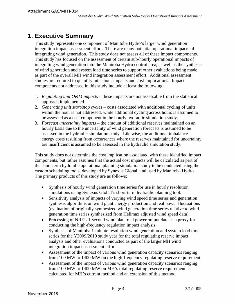
1. Executive SummaryThis study represents one component of Manitoba Hydro’s larger wind generationintegration impact assessment effort. There are many potential operational impacts ofintegrating wind generation. This study does not assess all of these impact components.This study has focused on the assessment of certain sub-hourly operational impacts ofintegrating wind generation into the Manitoba Hydro control area, as well as the synthesisof wind generation and system load time series to support other evaluations being madeas part of the overall MH wind integration assessment effort. Additional assessmentstudies are required to quantify inter-hour impacts and cost implications. Impactcomponents not addressed in this study include at least the following:
1. Regulating unit O&M impacts – these impacts are not assessable from the statisticalapproach implemented.
2. Generating unit start/stop cycles – costs associated with additional cycling of unitswithin the hour is not addressed, while additional cycling across hours is assumed tobe assessed as a cost component in the hourly hydraulic simulation study.
3. Forecast uncertainty impacts – the amount of additional reserves maintained on anhourly basis due to the uncertainty of wind generation forecasts is assumed to beassessed in the hydraulic simulation study. Likewise, the additional imbalanceenergy costs resulting from occurrences where the reserves maintained for uncertaintyare insufficient is assumed to be assessed in the hydraulic simulation study.
This study does not determine the cost implication associated with these identified impact components, but rather assumes that the actual cost impacts will be calculated as part of the short-term hydraulic operational planning simulation study to be conducted using the custom scheduling tools, developed by Synexus Global, and used by Manitoba Hydro. The primary products of this study are as follows:
• Synthesis of hourly wind generation time series for use in hourly resolutionsimulations using Synexus Global’s short-term hydraulic planning tool.
• Sensitivity analysis of impacts of varying wind speed time series and generationsynthesis algorithms on wind plant energy production and real power fluctuations(evaluation of originally synthesized wind generation time series relative to windgeneration time series synthesized from Helimax adjusted wind speed data).
• Processing of NREL 1-second wind plant real power output data as a proxy forconducting the high-frequency regulation impact analysis.
• Synthesis of Manitoba 1-minute resolution wind generation and system load timeseries for the Y2009/2010 study year for the total regulating reserve impactanalysis and other evaluations conducted as part of the larger MH windintegration impact assessment effort.
• Assessment of the impact of various wind generation capacity scenarios rangingfrom 100 MW to 1400 MW on the high-frequency regulating reserve requirement.
• Assessment of the impact of various wind generation capacity scenarios rangingfrom 100 MW to 1400 MW on MH’s total regulating reserve requirement ascalculated for MH’s current method and an extension of this method.
Page 4 3/1/2005
Attachment GAC/MH I-014
November 2013

Manitoba Hydro Wind Integration Sub-Hourly Operational Impacts Assessment
• Analysis of the impact on 10-minute changes in system net load for various wind capacity scenarios ranging from 250 MW to 1400 MW.
• Assessment of the potential TRM impact to accommodate the fluctuations in net system load that might result in additional tie-line flows.
1.1 Wind Generation Time Series Synthesis Hourly resolution wind generation time series were synthesized for 3 projected Manitoba wind plants based on metrological data collected at the 3 Manitoba sites. The approach utilized to synthesize the projected wind plant real power output time series is based on using a steady-state wind turbine generator power curve with the single mast metrological time series data. Adjustments are made for height differentials, air density, and various losses. The algorithm utilized is simple relative to meso-scale numeric weather prediction based approaches, but yields reasonable results that include the full range of variability of wind plant output needed to assess potential impacts. In general, the approach utilized yields power fluctuations that are more severe than seen in an actual wind plant, primarily because the model does not represent the full extent of intra-plant diversity that exists in actual wind plants. This results in steeper ramp rates and increased fluctuations, which provided a slightly conservative result when assessing the impacts of wind generation on net load variability. Due to differences in the wind generation estimation approach, the hourly time series synthesis performed for this study yielded slightly higher (42.3% vs. 38.9% for St. Leon) capacity factors than were calculated in a parallel study performed by Helimax. Comparison of the two separate approaches shows that there are several factors that result in this difference in calculated energy yield, with the primary factor being the lack of direct treatment of wake losses in the approach utilized in this study. In further analysis and comparison of the outputs of the two approaches, it was verified that inclusion of a treatment of wake losses provided capacity factor results that were within 1%. It was also shown that the impacts of relatively slight variations in the source meteorological data to produce a more representative “wind year” did not significantly impact the real power fluctuations obtained from the wind plants. With the confidence provided by these validation analyses, the hourly resolution wind plant time series were approved as inputs to the subsequent MH short-term hydraulic operations planning simulation study. In addition to the hourly resolution wind generation time series, 4-second and 1-minute resolution time series were required for integration impact assessment activities. These higher resolution time series were obtained by utilizing proxy data of actual wind plant output measurements obtained from NREL. The higher-resolution fluctuations inherent in this proxy data were isolated and scaled appropriately to represent the fluctuations of wind plants of the desired rated capacities utilized in the study scenarios. These scaled high-resolution fluctuations were then superimposed onto other appropriately scaled smoother variation components of the synthesized hourly resolution data from the projected Manitoba sites. This process yielded 1-minute and 4-second resolution wind generation time series for various wind capacity scenarios needed to analyze various potential wind integration impacts, including the high-frequency regulating reserve impacts and total regulating reserve impact analyses conducted as part of this study.
Page 5 3/1/2005
Attachment GAC/MH I-014
November 2013

Manitoba Hydro Wind Integration Sub-Hourly Operational Impacts Assessment
Similar processes were utilized to obtain 1-minute resolution load time series for the future study year based on load growth estimate provided by Manitoba Hydro.
1.2 High-Frequency Regulation Impact The 1-minute resolution wind generation and system load time series data for the projected wind plant capacities and future study year were utilized to assess the impact of wind generation on the high-frequency regulating reserve requirement for tracking the minute-to-minute variations in net load and maintaining the desired NERC compliance. The approach utilized for the assessment is based on the decomposition of system net load into a high-frequency fluctuation component and a slower varying ramping component. The intent of the decomposition is to allow quantification of the reserve required for system regulation. A fundamental assumption underlying this approach is that on-line units are re-dispatched every 5-10 minutes to follow longer-term ramping of system net load. As such, the regulating reserve requirement would be associated with the high-frequency variations. Manitoba Hydro does not operate their predominantly hydro system in this manner, but rather they attempt to bring additional hydro units on-line at optimal generating points to most efficiently utilize available water. As such, MH maintains total regulating reserves, comprising both spinning and non-spinning capacity, for tracking high-frequency fluctuations and longer-term ramping of system net load. As such, the high-frequency regulating reserve impact assessment does not represent the total impact to MH’s regulating reserve burden, but rather represents only the impact to the portion of Manitoba Hydro’s total regulating reserve requirement that is utilized to track the minute-to-minute, random variations in system net load.
The analysis conducted shows that the integration of wind generation ranging in capacity from 100 MW to 1400 MW would increase the high-frequency regulating reserve requirement 1.5% - 11% above that for system load alone. A key assumption of the analytical approach was that the high-frequency fluctuation in output of wind turbines within the same wind plant is statistically uncorrelated. This assumption is not completely accurate as there is a small, positive correlation between the output of turbines within close proximity. Sensitivity analysis of the high-frequency impact results to the within-plant correlation assumptions show that the impacts calculated for the 0% correlation assumption may double if an exaggerated intra-plant correlation level is assumed. Even with these unrealistic correlation levels, the impact on high-frequency regulation requirements for the highest penetration scenario of 1400 MW at a single site is an increase of approximately 10 MW above that required for load alone, or approximately a 20% increase.
1.3 Total Regulating Reserve Requirement Impact Manitoba Hydro is currently ahead of most North American utilities in the sense that Manitoba currently calculates the amount of total regulating reserve carried for different load periods -- hour of the day and month of the year -- rather than simply carrying a fixed reserve amount for all hours irrespective of expected total load magnitude or variability. The 1-minute resolution wind generation and system load time series data for the projected wind plant capacities and future study year were also utilized to assess the impact of wind generation on Manitoba Hydro’s total regulating reserve requirement.
Page 6 3/1/2005
Attachment GAC/MH I-014
November 2013

Manitoba Hydro Wind Integration Sub-Hourly Operational Impacts Assessment
This total regulating reserve requirement comprises both spinning and non-spinning capacity and is maintained for tracking high-frequency fluctuations and longer-term ramping of system net load. The approach implemented to quantify this impact is based on Manitoba Hydro’s internal total regulating reserve requirement calculation. The currently utilized method is referred to as the Hourly Total Regulating Reserve Method –CP85 (HTRRM – CP85). This method allocates reserves to cover 85% of the maximum variations of 4-second load from the corresponding hourly average for each clock hour of the day in each calendar month. This approach results in a 12 x 24 matrix of total regulating reserve requirement values calculated from at least one year of historical data. The first quantification of the impact of wind generation on total regulating reserve requirement utilized this HTRRM-CP85 method to calculate the reserve matrix for load alone and for system net load for each of the 23 wind capacity scenarios, with the impact determined as the increase in the total regulating reserve requirement. The average impact on any given hour was found to range from 9 MW – 69 MW for wind generation capacities of 250 MW – 1000 MW at a single site.
In reviewing the adequacy of the current HTRRM – CP85 method under increasing wind penetration levels, it was recognized that the probability of relatively large changes in net load increase rapidly as wind penetration levels increase as a percentage of system peak load. The HTRRM – CP85 method does not capture the impact of the larger reserve deficits associated with these more extreme net load changes or the potential for associated degradation of NERC performance criteria. Furthermore, Manitoba Hydro noted that it might have to alter its current operating procedures so as to ensure that the magnitudes of inadvertent interchanges with its tie-line neighbors do not significantly increase and to maintain NERC control performance criteria at existing levels. Consequently, an extension of the current HTRRM method was utilized to assess the additional reserve required to maintain a specified MW magnitude differential between the reserve value and the largest anticipated fluctuation magnitude (HTRRM-Equivalent Residual) as compared to the current criteria of expected percent of the time for which the magnitude of fluctuations exceeds reserves. Consequently, the impact on total regulating reserve requirement was also assessed as the additional reserves as calculated from the extended HTRRM -Equivalent Residual method to provide a range of potential impacts. This method yielded an average impact on even given hour in the range of 21 MW – 180 MW for wind generation capacities of 250 MW – 1000 MW at a single site. The higher calculated values using the HTRRM – Equivalent Residual method result from the fact that extreme deviations in wind plant output are more probable on a per unit basis than load deviations. The HTRRM – Equivalent Residual method focuses on the extremities of the net load deviation probability distributions where the integration of wind generation pushes these extremities out farther than it does the more central portions of the distributions such as the CP85 point.
1.4 Analysis of 10-Minute Changes in Net Load The probability distributions of the change in Manitoba Hydro (MH) load, wind generation, and MH system net load (load –wind generation) that occur over a 10-minute period were created. These distributions are constructed from the 1-minute resolution Y2009/2010 MH system load and projected wind plant real power output time series.
Page 7 3/1/2005
Attachment GAC/MH I-014
November 2013

Manitoba Hydro Wind Integration Sub-Hourly Operational Impacts Assessment
The “10-minute change” of the various quantities was determined according to two methods:
• Change in 10-min average value. The 1-minute resolution data is aggregated toyield a 10-minute average time series from which the 10-minute change isdetermined as the difference of one 10-minute average value and the previous 10-minute average value.
• Change in 1-min average value over 10-minute period. The source 1-minuteresolution time series described above are utilized to calculate the 10-minutechange as the difference in a specific 1-minute average value and the 1-minuteaverage value occurring 10 minutes prior.
It was found that the addition of wind increases the probability of occurrence of the most significant net load changes. For example, the magnitude of the 10-minute net load change that is expected 99% of the time increases by a factor of 2 for 1000 MW of wind and by a factor of 2.5 for 1400 MW of wind.
The change in the system net load over a 10-minute period has several potential implications for system operators. As noted previously, the 10-minute change in system load impacts the total regulating reserves to be held by MH. Although discussed in more detail in Section 5.4, the 10-minute change in net load can contribute to increasing ACE values and possibly impact the tie line capacity that is reserved to maintain reliability margins. Additionally, the 10-minute change in system net load can have implications on contingency reserves, emergency calls to reserve sharing pools, and NERC disturbance control performance.
1.5 TRM Impact Manitoba Hydro does not currently reserve additional TRM to accommodate the fluctuations of system net load. The impacts of wind generation on the magnitude of the sub-minute and multi-minute fluctuations of net load (load minus wind generation) were analyzed to determine whether the change in the magnitude and frequency of fluctuations that might impact tie line flows is significant enough to warrant holding additional TRM to accommodate net load fluctuations.
It was found that the impact of even high penetration wind generation scenarios on the sub-minute fluctuations is quite small with the worst case scenario showing a 3.35% increase in the standard deviation of the net load sub-minute fluctuation distribution. Thus, it is unlikely that additional TRM would be required on the basis of the impact on sub-minute fluctuations that might flow on the tie lines.
Analysis of a small subset of MH interchange data values indicates that some portion of the longer trending (10-minute) of MH load changes are coupled into the tie line interchange. As such, the previous analysis of impacts of wind generation on MH TRM based on the increased intra-minute fluctuation of the net system load likely does not completely represent the impacts that wind generation might have on TRM. Comparison of the changes in load relative to net load with the 500 MW/1-site wind plant for both
Page 8 3/1/2005
Attachment GAC/MH I-014
November 2013

Manitoba Hydro Wind Integration Sub-Hourly Operational Impacts Assessment
methods shows that the 10-minute fluctuations in wind plant real power output will increase the standard deviation and middle quartiles of the 10-minute net load fluctuations on the order of 25%-33%. The 500 MW of wind generation will increase the extreme (CP01 and CP99) 10-minute net load fluctuations on the order of 30%-50%. Furthermore, it was found that for higher penetration levels the extremities of the net load 10-minute change distribution spread even further with the CP01 and CP99 values increasing by a factor of 2-3 and the CP0.1 and CP99.9 values increasing by a factor of 2-4. The extent to which any of these fluctuations actually flow on the tie lines isdependent on the quality of total regulating reserves maintained and on the tuning of the AGC algorithm. If AGC is tuned to perfectly control generation to track net load changes on the order of several minutes, none of the 10-minute fluctuations will show on the ties. If, however, AGC is tuned to control more loosely, some portion of the fluctuations may show on the ties. It was found that for the absolute worst case scenario of no control of 10-minute fluctuations, the flows on the ties resulting from these flows would increase on the order of 1.5-3 times. Based on discussions with MH personnel and internal analysis of a small set of tie line flow data, it is expected that given the current AGC tuning, a relatively small portion of the total 10-minute changes will actually flow on the ties. MH system operators will have to make a decision as to whether the increased tie line flows on might warrant reserving tie line capacity.
Page 9 3/1/2005
Attachment GAC/MH I-014
November 2013

Manitoba Hydro Wind Integration Sub-Hourly Operational Impacts Assessment
2. IntroductionNote that Manitoba Hydro has developed a wind integration studies glossary to helppromote consistent terminology across the various wind integration assessment activitiesbeing conducted. This glossary is included in Appendix 1. An attempt has been made toconform the terminology of this report to the glossary in Appendix 1.
2.1 Study Background Manitoba Hydro first contacted Electrotek regarding potentially conducting a wind integration operational impacts study in May 2003. These initial discussions focused on obtaining a preliminary estimate of wind impacts utilizing limited data available at the time, realizing that a more rigorous investigation might be necessary at a later time. Subsequent to these preliminary discussions, Manitoba Hydro released a competitive request of proposal (RFP) in October 2003 to conduct a wind integration operational impacts study. The RFP called for an analytical approach that included time domain simulations on various operational time frames including 1-hour resolution (scheduling/uncertainty), 5-minute resolution (intra-hour load following), and 4-second-resolution (regulation) simulations. As a trade-off between the rigor of the analytical method and perceived cost expectations, Electrotek responded to this RFP proposing a simplified analysis approach that combined a statistical evaluation of certain intra-hour impacts and time domain simulation of other longer-term impacts.
After reviewing Electrotek’s response to the RFP, MH personnel determined that in order to determine the impacts on its short term hydraulic operations, the time-domain hourly operations simulation portion of the study could most effectively be conducted using Synexus Global’s short-term hydraulic operational planning tool in a joint effort between MH and the developer of the planning tool. As such, this portion of the integration effort was removed from the proposed Electrotek work scope and a contract to conduct the remaining analyses was executed at the end of January 2004.
2.2 General Analytical Approach Characteristics The analytical framework adopted for this study attempts to disaggregate the integrated process of operating and controlling control area resources into various time frames in which various control actions are taken. Figure 1 provides a graphical representation of this decomposition of the impact component time frames and the control actions implemented to maintain an acceptable balance between control area generation and control area supply requirements. In actuality, the operational and control process is integrated with manual actions of system operators interspersed with automatic control actions such as the Load Frequency Control and Economic Dispatch algorithms that may be implemented as part of the AGC. Accurately modeling this integrated process would require tools specific to MH operations and an intimate knowledge of MH operational practice. The simplified disaggregated approach is taken in an attempt to quantify the technical and economic impacts of the incremental control actions that must be undertaken to maintain a comparable level of system performance with the integration of large capacities of wind generation.
Page 10 3/1/2005
Attachment GAC/MH I-014
November 2013

Manitoba Hydro Wind Integration Sub-Hourly Operational Impacts Assessment
tens of minutes to hours
LoadFollowing
seconds to minutes
Regulationdays
Daily/Hourly Scheduling
LFCUnit
GovenorResponse
EconomicDispatch
Real-TimeOperatorActions
UnitCommitment
TimeResolution of
Service/Control
Figure 1. Illustration of impact component time frames and associated control actions implemented to maintain acceptable balance of supply and demand.
The operational time frames of Figure 1 are further defined as follows:
• Regulation Component (also referred to as high-frequency regulation) deployingfast responding units on AGC to compensate for the uncorrelated, high-frequency(minute-to-minute) variations of net load.
• Load Following Component commitment and dispatch of generation to followslower, correlated variations in net load through daily load cycle.
o Intra-hour – dispatch of on-line units within hourly pre-scheduleo Inter-hour – cycling of units in (half-) hourly unit schedule to meet generation
requirements for current-day schedule horizon• Scheduling/Unit Commitment short-term planning horizon (1-day to 1-week for
thermal systems and potentially longer for hydro systems) upon which thermal unitsare committed or water is scheduled and upon which transactions made to meet loadforecasts and other requirements
It should be noted that the actual delineation between the regulation component and load following component can be arbitrary. Much of the literature on deregulated electricity markets defines the differentiation as we have above, where the regulation component includes the fast, uncorrelated variations of net load and the load following component includes the slower, correlated variations of net load. This delineation is based in the operation of deregulated electricity markets where the system operator procures sufficient regulating capacity to track the variations around estimated load over the next 5-10 minute interval. At the end of each of these regulating period intervals, it is assumed that
Page 11 3/1/2005
Attachment GAC/MH I-014
November 2013

Manitoba Hydro Wind Integration Sub-Hourly Operational Impacts Assessment
system operators will perform a dispatch of the on-line economic resources to follow the sub-hourly movements of the correlated load variations. As such, the reserve carried by participants in a deregulated market to track the regulation component by does not need to include a component for sub-hourly load following. As will be noted in subsequent sections, Manitoba Hydro operates its own control area and does not directly participate in a deregulated electricity market, where all the generation within the market is controlled by the market operator. Manitoba Hydro is an external participant in these deregulated electricity markets, and this status as an external participant essentially limits Manitoba Hydro to hour ahead transactions in the real time or the day ahead markets. Variation within the hour must be absorbed within the Manitoba Hydro system in order to maintain the constant exports schedules with the markets. Therefore, Manitoba Hydro maintains a total regulating reserve requirement for the one hour period that includes additional capacity (both online and off-line) for load following that is not necessarily required for participants within a deregulated market who only need to cover variations within the next 5-10 minutes with their reserve. With the impact component time frames defined as stated, various analytical methods are utilized to quantify the impacts of wind generation on operation and control in each time frame. The underlying assumption is that additional high-frequency regulating reserves are held in order to maintain system performance at a comparable level as before the additional variations from wind generation is integrated. Once this basic performance criterion is met on the regulation component time frame, longer time frame impacts are assessed such as the additional total regulating reserve requirement. The increase in total regulating reserve is then passed on to the short-term hydraulic operational planning tool for a cost analysis study by the tool developer. The short-term hydraulic operational planning tool study can quantify the costs of the additional total regulation reserve, as well any costs resulting from any sub-optimization of the hydro resources resulting from the wind intermittency. The methods utilized in this study for determining additional reserve capacities for regulation, load following, and TRM are statistical methods. These methods require the development of probability distributions of fluctuations on the defined time frames from time series data. Additional reserves to accommodate the integration of wind generation are then quantified by determining the capacity required to maintain a comparable percentage of fluctuations or range of fluctuation not covered. Such statistical approaches are simplifications of the actual integrated time-domain control processes described previously. Another approach to quantifying reserves is through time domain simulations of actual system operations utilizing the underlying time series data sets rather than statistically comparing distributions developed from the time series data. The time-domain simulation approach requires a much more representative model of the specific operational procedures of the control area. When modeled appropriately, however, time-domain simulations are a more rigorous and representative approach to determining system impacts.
Page 12 3/1/2005
Attachment GAC/MH I-014
November 2013

Manitoba Hydro Wind Integration Sub-Hourly Operational Impacts Assessment
2.3 Study Scope
2.3.1. Potential Impacts There are many potential technical and economic impacts of adding additional variability and uncertainty to system operations such as occurs with the integration of wind generation. Short-term operations and control impacts that might be quantified include:
• Transmission Reliability Margin additional tie-line capacity that must be withheldin order to accommodate the fluctuation in net system load that is not completelycontrolled by AGC. The cost of MH maintaining additional TRM reserve would berealized as the opportunity costs of potential lost energy transactions.
• Regulation Component additional spinning capacity on online units that are underAGC.
o Reserve costs – maintaining additional regulating reserve to maintainacceptable NERC system performance increases operating costs or reducesrevenues from energy transactions.
o O&M costs – additional high-resolution fluctuations will likely increase theduty on regulating units as magnitude of deviations and frequency of changein direction of fluctuations increases.
• Load Following Component because it is possible that wind generation canincrease the ramping requirements to follow longer-term trends in net system load,the costs associated with committing and dispatching generating units to follow thedaily net load cycle can also increase. These costs may include additional operatingcosts due to less optimal dispatch of online units (or operating hydro units off bestgate) or increasing the number of unit start/stop cycles. These costs are oftendecomposed into intra-hour and inter-hour components as noted previously.
o Intra-hour LF – additional operating costs associated with less optimaldispatch of online units (economic dispatch in thermal system) or operatinghydro units off best gate, starting/stopping un-scheduled units within hour tofollow sub-hourly load trends, or additional capacity that must be reserved tofollow sub-hourly ramping of net load
o Inter-hour LF – additional operating costs associated with less optimalscheduling or additional cycling of units to meet hourly trending of net load
• Forecast Uncertainty additional reserve and imbalance energy costs resulting fromday-ahead and/or hour-ahead wind generation forecast error in scheduling
2.3.2. Impacts Specifically Assessed in this Study This study does not assess all of these impact components. Some components are assumed to be quantified in other studies. For example, all of the impacts incurred on an hourly or longer time frame are assumed to be assessed in the short-term hydraulic operational planning simulation study to be conducted using the custom scheduling tools, developed by Synexus Global, and used by Manitoba Hydro, as noted in the Study Background (section 2.1). Other impact components, such as the increased duty on regulating units, are omitted entirely in this study. To ensure clarity as to the scope of impact components assessed in the study, they are listed as follows:
Page 13 3/1/2005
Attachment GAC/MH I-014
November 2013

Manitoba Hydro Wind Integration Sub-Hourly Operational Impacts Assessment
1. High-frequency regulating reserves – the impact on the high-frequency regulating reserve component of MH’s total regulating reserve that must be maintained as capacity on spinning units under AGC to cover the high-resolution fluctuation in net system load is assessed. (It should be noted that MH maintains additional sub-hourly spinning reserves on AGC for intra-hour load following. )
2. Total regulating reserves – the impact on total regulating reserve (high-frequency regulation component reserves+ load following component reserves for ramping of load within the hour, which includes the sub-hourly LF and some portion of the inter-hour load following) that is withheld from potential market transactions for the hour.
3. TRM reserves – impact on sub-minute and 10-minute fluctuations of net system load that might influence Manitoba’s existing Transmission Reliability Margin calculations.
This study does not determine the cost implication associated with these identified impact components, but rather assumes that the actual cost impacts will be calculated as part of the short-term hydraulic operational planning simulation study to be conducted using the custom scheduling tools, developed by Synexus Global, and used by Manitoba Hydro. Impact components not addressed in this study include at least the following: 1. Regulating unit O&M impacts – these impacts are not assessable from the statistical
approach implemented and are difficult to quantify. 2. Load Following unit start/stop cycles – costs associated with additional cycling of
units within the hour is not addressed, while additional cycling across hours is an hourly resolution assessment not within the defined scope of this study.
3. Forecast uncertainty impacts – the amount of additional reserves maintained on an hourly basis due to the uncertainty of wind generation forecasts was not within the defined scope of this study. Likewise, the additional imbalance energy costs resulting from occurrences where the reserves maintained for uncertainty are insufficient was not within the defined scope of this study.
It should be noted that in addition to conducting the impact calculations and reporting the results, a significant deliverable of this study is provision of the required wind generation time series, system load times series, and total regulating reserve requirement matrices in electronic form for use in the hydraulic simulations to be conducted subsequently to determine cost implications.
Page 14 3/1/2005
Attachment GAC/MH I-014
November 2013
Manitoba Hydro Wind Integration Sub-Hourly Operational Impacts Assessment
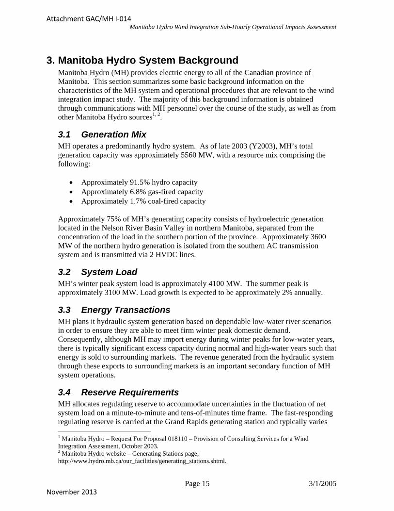
3. Manitoba Hydro System BackgroundManitoba Hydro (MH) provides electric energy to all of the Canadian province ofManitoba. This section summarizes some basic background information on thecharacteristics of the MH system and operational procedures that are relevant to the windintegration impact study. The majority of this background information is obtainedthrough communications with MH personnel over the course of the study, as well as fromother Manitoba Hydro sources1, 2.
3.1 Generation MixMH operates a predominantly hydro system. As of late 2003 (Y2003), MH’s totalgeneration capacity was approximately 5560 MW, with a resource mix comprising thefollowing:
• Approximately 91.5% hydro capacity• Approximately 6.8% gas-fired capacity• Approximately 1.7% coal-fired capacity
Approximately 75% of MH’s generating capacity consists of hydroelectric generation located in the Nelson River Basin Valley in northern Manitoba, separated from the concentration of the load in the southern portion of the province. Approximately 3600 MW of the northern hydro generation is isolated from the southern AC transmission system and is transmitted via 2 HVDC lines.
3.2 System Load MH’s winter peak system load is approximately 4100 MW. The summer peak is approximately 3100 MW. Load growth is expected to be approximately 2% annually.
3.3 Energy Transactions MH plans it hydraulic system generation based on dependable low-water river scenarios in order to ensure they are able to meet firm winter peak domestic demand. Consequently, although MH may import energy during winter peaks for low-water years, there is typically significant excess capacity during normal and high-water years such that energy is sold to surrounding markets. The revenue generated from the hydraulic system through these exports to surrounding markets is an important secondary function of MH system operations.
3.4 Reserve Requirements MH allocates regulating reserve to accommodate uncertainties in the fluctuation of net system load on a minute-to-minute and tens-of-minutes time frame. The fast-responding regulating reserve is carried at the Grand Rapids generating station and typically varies
1 Manitoba Hydro – Request For Proposal 018110 – Provision of Consulting Services for a Wind Integration Assessment, October 2003. 2 Manitoba Hydro website – Generating Stations page; http://www.hydro.mb.ca/our_facilities/generating_stations.shtml.
Page 15 3/1/2005
Attachment GAC/MH I-014
November 2013

Manitoba Hydro Wind Integration Sub-Hourly Operational Impacts Assessment
between 40- 50 MW. The longer-term load-following component of the regulating reserve requirement is determined for each hour of the day on a monthly basis from a statistical calculation of historical fluctuations of system load. This calculation process is described in detail in section 5.2. Although some portion of the load-following component of regulating reserve may be carried at Grand Rapids, the balance of this reserve is carried on the HVDC system from the northern hydroelectric generating stations.
Page 16 3/1/2005
Attachment GAC/MH I-014
November 2013

Manitoba Hydro Wind Integration Sub-Hourly Operational Impacts Assessment
4. Wind Plant Modeling and Interaction with System LoadThe Manitoba Hydro wind generation impact assessment project requires windgeneration and system load data on three different time resolutions:
1. regulation time frame – high-frequency data on the order of several seconds up to1-minute for assessment of the high-frequency regulating reserve impact
2. load-following time frame – 1-10 minute resolution data for assessment ofimpacts on following sub-hourly trends in load
3. scheduling time frame – hourly resolution data to be utilized in schedulingsimulations conducted by another contractor utilizing the custom scheduling tools,developed by Synexus Global, and used by Manitoba Hydro.
Given that this assessment is being made for wind plants that do not yet exist and for the Manitoba Hydro Y2009/2010 system load, measured data is unavailable for these quantities. The models and methods used to obtain the wind generation and load data utilized for the various aspects of this study are described in the following subsections. The impact assessments are made for varying wind penetration levels in the MH Y2009/2010 load year. For the analyses conducted, multiple wind generation time series for varying total wind generation capacities are utilized, but a single MH system load series for the study year is utilized.
4.1 Scheduling Time Frame (1-hour resolution) The hydraulic simulations to be conducted for the scheduling impact analysis by the other contractor requires concurrent hourly resolution wind generation and system load chronological time series data. This subsection describes the models utilized for obtaining these data sets.
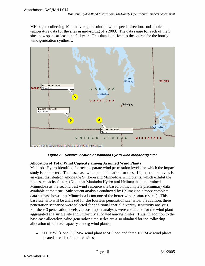
4.1.1. Wind Model Data Source Since the proposed wind generation does not yet exist, MH does not have a historical record of wind plant production for the various sites that might be developed for wind generation. MH does, however, have a database of meteorological data for at least three potential development sites in the region. These three wind sites are
• St. Leon (also referred to as Lizard Lake)• Boissevain• Minnedosa
The relative location of these sites is shown in Figure 2. These sites are almost equidistant with the distances between sites as follows:
St. Leon – Boissevain --> 76 miles (122 km) Boissevain – Minnedosa --> 62 miles (100 km) Minnedosa – St. Leon --> 89 miles (143 km)
Page 17 3/1/2005
Attachment GAC/MH I-014
November 2013
Manitoba Hydro Wind Integration Sub-Hourly Operational Impacts Assessment
MH began collecting 10-min average resolution wind speed, direction, and ambient temperature data for the sites in mid-spring of Y2003. The data range for each of the 3 sites now spans at least one full year. This data is utilized as the source for the hourly wind generation synthesis.
Figure 2 – Relative location of Manitoba Hydro wind monitoring sites
Allocation of Total Wind Capacity among Assumed Wind Plants Manitoba Hydro identified fourteen separate wind penetration levels for which the impact
data
e
t
• 500 MW one 500 MW wind plant at St. Leon and three 166 MW wind plants located at each of the three sites
study is conducted. The base case wind plant allocation for these 14 penetration levels is an equal distribution among the St. Leon and Minnedosa wind plants, which exhibit the highest capacity factors (Note that Manitoba Hydro and Helimax had determined Minnedosa as the second best wind resource site based on incomplete preliminary available at the time. Subsequent analysis conducted by Helimax on a more complete data set has shown that Minnedosa is not one of the better wind resource sites.). This base scenario will be analyzed for the fourteen penetration scenarios. In addition, threpenetration scenarios were selected for additional spatial diversity sensitivity analysis. For these 3 penetration levels various impact analyses were conducted for the wind planaggregated at a single site and uniformly allocated among 3 sites. Thus, in addition to thebase case allocation, wind generation time series are also obtained for the following allocation of relative capacity among wind plants:
Page 18 3/1/2005
Attachment GAC/MH I-014
November 2013

Manitoba Hydro Wind Integration Sub-Hourly Operational Impacts Assessment
• 1000 MW one 1000 MW wind plant at St. Leon and three 333 MW windplants located at each of the three sites
Note th lit between various anitoba Hydro data sites may not completely represent the potential spatial diversity
vide
nts)Base Case Allocation Diversity Allocation
• 1400 MW one 1400 MW wind plant at St. Leon and three 466 MW windplants located at each of the three sites
at this assumed diversity obtained from the proposed spMeffect that would exist for Manitoba Hydro total wind plant production, but will prosome representation of the spatial diversity achieved from multiple project sites. The wind plant allocation for all of the scenarios to be studied is summarized in Table 1.
Table 1. Summary of wind plant allocation for studied penetration levels
Total WindPlant Capacity St. Leon Minn. Boiss. St. Leon Minn. Boiss. St. Leon Minn. Boiss.
100 50.0 50.0 0.0 -- -- -- -- -- --200 100.0 100.0 0.0 -- -- -- -- -- --250 125.0 125.0 0.0 -- -- -- -- -- --400 200.0 200.0 0.0 -- -- -- -- -- --500 250.0 250.0 0.0 500.0 0.0 0.0 166.7 166.7 166.7600 300.0 300.0 0.0 -- -- -- -- -- --750 375.0 375.0 0.0 -- -- -- -- -- --800 400.0 400.0 0.0 -- -- -- -- -- --900 450.0 450.0 0.0 -- -- -- -- -- --1000 500.0 500.0 0.0 1000.0 0.0 0.0 333.3 333.3 333.31100 550.0 550.0 0.0 -- -- -- -- -- --1200 600.0 600.0 0.0 -- -- -- -- -- --1300 650.0 650.0 0.0 -- -- -- -- -- --1400 700.0 700.0 0.0 1400.0 0.0 0.0 466.7 466.7 466.7
Diversity Allocation(Three Wind Pla(Two Wind Plants) (One Wind Plant)
Data Augmentation (Filling Data Gaps) he archived 10-minute data for the three sites was obtained from the contractor that
data consists of wind speed and direction at as
The
s of the
caled based on average wind shear coefficient calculated for the site from measurements.
TManitoba uses for collecting the data. Thisthree anemometer heights (10m, 40m, and 60m) and ambient temperature. This data wreceived in 3 separate data sets via FTP. The contractor stated that the data sets had already undergone quality control as part of the larger collection program. Thus, the quality of the data (i.e., absence of unreasonable values) is assumed to be sufficient. data was analyzed, however, to determine the extent of data coverage (i.e., gaps withinthe data). The 60-meter tower measurements were utilized as the base data quantities since these measurements are nearest in height to that of typical hub heights for commercially available turbines. The coverage of the 60m data was found to vary per site with multiple data gaps ranging from a few hours to several days. The resultdata coverage analysis for each site are provided in Table 2, Table 3, and Table 4, respectively. These tables also state the method used to fill the data gaps. The preferred methods of filling the gaps in descending order of priority were as follows:
1. Replace 60m data with concurrent 40m-anemometer measurement, s
2. Replace 60m data with concurrent 10m-anemometer measurement, scaled basedon average wind shear coefficient calculated for the site from measurements.
Page 19 3/1/2005
Attachment GAC/MH I-014
November 2013

Manitoba Hydro Wind Integration Sub-Hourly Operational Impacts Assessment
3. If neither the 40m or 10m concurrent measurements were available, 60m datapoints corresponding to the same values for the time period just prior to the data
4. ts.
issing Data
12/27/03 10:00 1/11/04 12:00 2173 Same time period from previous data1/14/04 0:00 1/14/04 17:50 108 Same time period from previous data
1/14/04 21:20 1/21/04 14:30 Scale 10m Anemometer1/21/04 14:40 1/31/04 23:50 Scale 40m Anemometer
2/1/04 0:10 2/1/04 20:10 121 Scale 40m Anemometer2/17/04 13:40 2/17/04 22:30 54 Scale 10m Anemometer3/3/04 14:40 3/3/04 14:40 1 Scale 40m Anemometer3/3/04 15:00 3/3/04 15:10 2 Scale 40m Anemometer3/4/04 6:10 3/4/04 7:10 Scale 40m Anemometer3/4/04 7:20 3/4/04 13:30 Scale 10m Anemometer
3/18/04 13:40 3/18/04 13:40 1 Scale 40m Anemometer3/18/04 14:00 3/18/04 14:10 2 Scale 40m Anemometer
3/27/04 3:20 3/27/04 3:20 1Interpolate between surrounding 10-min points (scaling 40m value not consistent w/surrounding values)
3/27/04 3:40 3/27/04 3:40 1Interpolate between surrounding 10-min points (scaling 40m value not consistent w/surrounding values)
3/27/04 4:40 3/27/04 4:40 1Interpolate between surrounding 10-min points (scaling 40m value not consistent w/surrounding values)
3/27/04 5:00 3/27/04 5:00 1Interpolate between surrounding 10-min points (scaling 40m value not consistent w/surrounding values)
5/11/04 22:30 5/11/04 23:30 10m Anemometer (alpha=0.035 based on avg of previous 8 hrs)5/11/04 23:40 5/11/04 23:50 Same time period from previous data5/11/04 23:40 5/11/04 23:50 2 Same time period from previous data
2464
45
9
gap. For example, data from 1/14/04 00:00 to 11/14/04 17:50 is replaced withdata from 1/13/04 00:00 to 11/13/04 17:50 if original data exists without gaps.If data gap consists of only 1 or 2 points and context of data indicates that otheroptions do not provide good match, data replaced by interpolating between poin
Table 2. Data Coverage analysis for St. Leon site # Missing
Begin Data Gap End Data Gap Data Pts. Method for Replacing M
Table 3. Data Coverage analysis for Minnedosa site
Missing Data11/17/2003 9:40 11/18/2003 4:00 Same time period from previous data11/18/2003 5:00 11/21/2003 18:00 Scale 10m Anemometer12/26/2003 3:50 12/26/2003 3:50 1 Same time period from previous data
12/28/2003 19:00 12/28/2003 23:50 30 Same time period from previous data2/24/2004 0:10 2/24/2004 23:50 143 Scale 10m Anemometer
2/26/2004 2/26/2004 13:00 79 Scale 10m Anemometer3/2/2004 11:50 3/2/2004 12:30 5 Scale 10m Anemometer3/27/2004 2:00 3/27/2004 14:30 76 Same time period from previous data
627
# Missing Begin Data Gap End Data Gap Data Pts. Method for Replacing
Page 20 3/1/2005
Attachment GAC/MH I-014
November 2013

Manitoba Hydro Wind Integration Sub-Hourly Operational Impacts Assessment
Table 4. Data Coverage analysis for Boissevain site # Missing
Begin Data Gap End Data Gap Data Pts. Method for Replacing Missing Data
7/3/03 2:00 7/3/03 2:40 5 Same time period from previous data8/27/03 18:40 8/27/03 23:50 32 Same time period from previous data10/16/03 9:50 10/16/03 14:00 26 Scale 10m Anemometer
11/14/03 14:40 11/15/03 10:10 118 Scale 40m Anemometer1/15/04 12:40 1/15/04 23:50 68 Scale 10m Anemometer (alpha=-0.17)
3/2/04 9:20 3/2/04 9:20 1 Scale 10m Anemometer3/2/04 14:30 3/2/04 14:30 1 Scale 10m Anemometer3/2/04 15:10 3/2/04 15:10 1 Scale 40m Anemometer3/3/04 11:10 3/3/04 11:20 2 Scale 40m Anemometer3/3/04 11:50 3/3/04 11:50 1 Scale 10m Anemometer3/3/04 23:30 3/3/04 23:30 1 Scale 40m Anemometer3/5/04 0:10 3/5/04 0:10 1 Scale 40m Anemometer
3/14/04 18:50 3/14/04 19:00 2 Scale 40m Anemometer3/18/04 12:40 3/18/04 12:40 1 Scale 40m Anemometer
For the data filled by scaling the lower anemometer measurements, the scaling is performed according to Equation 1.
α
⎟⎟⎠
⎞⎜⎜⎝
⎛=
0HH
SS
o
(Equation 1)
where S is the hub height wind speed, S0 is the original measured wind speed, H is the new height, H0 is the original height, and α is the wind shear coefficient3. For each 10-minute data point for which data was available from multiple anemometer heights, a wind shear coefficient was calculated for that specific 10-minute measurement. The annual mean wind shear coefficients were then calculated for each site. These annual mean coefficients that were utilized for scaling the original raw 10-minute data points for each site and are shown in Table 5. Note that instances where the calculated mean coefficients did not appear correct for small data gaps, coefficients were calculated for smaller data subsets just prior to the data gap and used for filling the subsequent data gap. Such instances are noted in the data gap summary tables (Table 2, Table 3, and Table 4)
Table 5. Calculated mean wind shear coefficients per site for 1-year of data. Wind Data Site Mean Wind Shear Coeff. Std. Deviation
Boissevain 0.19436 0.12449 Minnedosa 0.18653 0.11767 St. Leon 0.20525 0.12451
Temporal Data Normalization The actual year for which the impact study is performed is the MH load year of 2009/2010, which spans 4/1/2009 through 3/31/2010. It is assumed that the wind regime
3 Minnesota Department of Commerce, 14th Wind Resource Analysis Program Report, October 2002.
Page 21 3/1/2005
Attachment GAC/MH I-014
November 2013
Manitoba Hydro Wind Integration Sub-Hourly Operational Impacts Assessment
for the source data period of spring 2003 through spring 2004 is unchanged for the study year. Note, however, that the MH system load obviously does change from the base year to the study year. MH personnel calculated a projected load series for the study year based on a process conducted internally by MH personnel. This process entails averaging of various potential load situations and provides a “typical” load year for the forecast years beyond 2 years in the future, which applies to our study year of Y2009/2010. This “typical” forecast series consists of an 8760 time series spanning 4/1/09 –4/1/10 and does not include “atypical” occurrences such as the additional day associated with leap years. The hourly scheduling simulations to be conducted by MH’s other contractor requires concurrent hourly resolution wind generation and load time series. This requirement necessitates two additional adjustments to the source wind resource data:
• Date range of source data varies for each of the three sites, with the starting dateranging from 4/10/2003 8:30:00 AM to 5/12/2003. The source wind resourcedata sets are therefore temporally synchronized with the load series by filling the“gap” at the beginning of each of the data sets with the data from the same timeperiod one year in the future. For example, the data range for the Minnedosa sitedata is #4/10/03 8:30# #5/2/04 18:50#. The Minnedosa data from the timeperiod #4/1/04 00:00# --> #4/10/04 8:20# is copied to the corresponding periodfor Y2003/2004 in order to have a time series that synchs with start time of theLoad Year, #4/1/03 00:00#. Since the load time series synthesis process destroysany correlations between specific meteorological events and resulting loadperturbations in the source data, the above process is believed to provide areasonable synchronization of the load and wind generation data. It should benoted that the process does inject an arbitrary discontinuity in the wind series atthe boundary between the original start time point and the preceding point. Thisdiscontinuity may manifest itself as an unusually large change in wind generationoutput from one time step to the next, but this single arbitrary delta should notimpact the overall analysis, as the changes in output will be analyzed statistically.
• The wind resource source data sets each span a leap year in February. Thus, thewind resource data must be synchronized such that the resulting wind generationtime series with the load series such that it does not contain data for one day morethan the study year load series. Consequently, the wind generation time series isadjusted by incrementing each day of the time series beginning at 2/29/04 by oneday, in affect removing the additional day. This approach provides datacontinuity while also synchronizing the wind generation time series with the loadseries.
4.1.2. Wind Generation Synthesis Model Utilizing the original wind resource data provided by Helimax for the three potential development sites and the data filling methods outlined in the previous section, a contiguous year of 10-min resolution wind speed, wind direction, and temperature data was obtained for each of the three sites. These meteorological data were used in conjunction with assumed wind plant project parameters to calculate projected wind
Page 22 3/1/2005
Attachment GAC/MH I-014
November 2013

Manitoba Hydro Wind Integration Sub-Hourly Operational Impacts Assessment
generation on a 10-minute resolution at each of the identified sites using the following general steps:
1. Adjust wind speed measurement based on relation of anemometer height to assumed turbine hub height
2. Calculate wind turbine output for single turbine based on assumed turbine power curve adjusting energy capture based on air density (temperature) and specified cold temperature cut-out for the turbine (see section “Analysis of Cold Weather Cut-Out Impact” for more information).
3. Calculate total wind plant output based on assumed number of turbines and an assumed scaling factor to represent collection system losses, various turbine losses, turbine availability, etc. Although there are many different sources of losses, the algorithm utilized for synthesizing wind generation for this effort aggregates all of these loss sources into a single scaling factor. There are certainly more accurate models for synthesizing wind generation that utilize physical models based on detailed climatology databases. Even these more sophisticated models do not explicitly address all of the loss sources separately, if at all. For instances were the wind plant already is in production, the models can be calibrated against historical data to provide better estimates of the total losses.
This general process is summarized in the flow chart shown in Figure 3.
Helimax 10-min
Met Data
FillData Gaps
CalculateAnnual MeanWind Shear
Coeffs.
Wind SpeedHeight
Adjustment
TurbinePower Curve
Calc w/AirDensity Adj.
Apply Loss Factorand Scale toWind Plant
Figure 3. Flow chart of hourly wind generation synthesis algorithm.
Based on the accuracy level required for this study and the resources available for the wind modeling task, the simplified approach utilized yields sufficient results. It should be noted that the model used typically estimates wind generation levels higher than those realized once the wind plant is operational primarily due to the lack of treatment of individual loss factors such as wake losses that are plant layout specific. Comparison of wind generation time series synthesized from an on-site anemometer measurement data using this method with actual wind generation real power output from an existing plant has shown that this method yields results that are 4-5% higher than actual measurements. Because many of the impacts to be assessed are associated with the magnitude of fluctuation of the wind generation, utilizing a wind generation synthesis model that errs on the high side yields conservative wind impact results (more significant).
Page 23 3/1/2005
Attachment GAC/MH I-014
November 2013

Manitoba Hydro Wind Integration Sub-Hourly Operational Impacts Assessment
Analysis of Cold Weather Cut-Out Impact The low temperature operating limit specified by turbine vendors is treated like the high-speed cutout of the turbine in that once the low temperature limit is reached the turbine output becomes zero. Turbine vendors likely can provide additional heating capability to lower this limit, but the analysis contained herein utilized the stated limit specified in response to an RFP from another Canadian utility. For the 10-min source data utilized, the cold weather operating limit affects approximately as many as 597 10-minute periods during the year for any one site. Both of the turbines simulated for the three sites in this study have cold temperature operating limits of –30 degrees Celsius. Table 6 lists the number of 10-minute periods affected for the source data year for each site. As expected, all of the occurrences occur during winter months, specifically in either January or February. The total number of periods affected represents approximately 1% of the year. The vast majority of the occurrences of any given site occur in groups when the temperature remains below the threshold temperature for many hours (sometimes days) at a time.
Table 6. Number of 10-minute periods during year affected by cold temperature limit. Site Jan Feb TotalSt. Leon 545 52 597 Minnedosa 487 16 503 Boissevain 378 69 447
Analysis of High Wind Cut-Out Impact When the high wind speed operating limit specified by turbine vendors is reached the turbine output becomes zero to avoid damage to the machine as it overspeeds. For the turbines identified for the Manitoba sites studied, the high-speed cut-out values are 44.7 mph (NM82 turbine at St. Leon and Boissevain) and 56.1 mph (GE15s at Minnedosa). For the 10-min source data utilized, the high speed operating limit affects very few 10-minute periods during the year for any one site. Table 7 lists the number of 10-minute periods affected for the source data year for each site. The total number of periods affected represents less than 0.01% of the year. Although many of the occurrences of high speed cutout for any given site occur in groups when the wind speed remains above the threshold for several hours at a time, there is a higher percentage of isolated occurrences of high speed cut-out as compared to the low temperature cut-out. The total number of occurrences is much less, however.
Table 7. Number of 10-minute periods during year affected by high speed cut-out. Site Mar May July Oct Nov Total St. Leon 25 1 0 2 1 29Minnedosa 0 0 0 0 0 0Boissevain 28 0 1 12 0 41
The above analysis should be considered in light of the following qualification. In selecting a turbine, the wind plant developers will consider the turbine cut-out speed relative to the wind regime at the site with the intent of maximizing availability. Also, for a given turbine, the actual steady-state power curve can vary somewhat based on
Page 24 3/1/2005
Attachment GAC/MH I-014
November 2013

Manitoba Hydro Wind Integration Sub-Hourly Operational Impacts Assessment
blade length selected and other factors. The wind developers and vendors will tweak the turbine specs, to the extent possible, to yield a power curve with a cut-out speed that doesn’t lie dead center of common wind speed range. The WTG specified for the St. Leon site was the NEG Micon NM82, which has a relatively low cut-out wind speed value of 47 mph (21 m/s). A power curve with a slightly higher cut-out speed would lessen the number of occurrences. For example, had we used the GE 1.5s turbine (used for Minnedosa) power curve (cut-out of 56.1 mph or 25.1 m/s) at St. Leon, there would be no high-speed cut-out occurrences for the 4/1/03 – 4/1/04 10-minute time series.
Data Adjustment to Hub Height The meteorological measurements in the source wind resource database from Helimax are all collected at a height of 60 meters above ground. The assumed hub heights of the wind turbines at the various locations are 65 m and 70 m, however. Because wind speed varies as a function of height, each measurement must be scaled appropriately to the assumed height of the wind turbines. All measurement data is scaled to the expected hub height of the wind turbines using Equation 1, repeated below, where S is the hub height wind speed, S0 is the original measured wind speed, H is the new height, H0 is the original height, and a is wind shear). Wind shear is a measure of the friction encountered by the wind as it moves across the ground, and is thus dependent upon surface roughness. The wind shear coefficient values utilized for the scaling are those mean values calculated and shown in Table 5.
α
⎟⎟⎠
⎞⎜⎜⎝
⎛=
0HH
SS
o
Equation 1
Power Output of Wind Turbine Based upon investigation of various modeling issues it can be shown that for resolutions greater than several seconds, a quasi steady-state model incorporating the wind turbine power curve is sufficient for developing wind turbine output data. MH personnel indicated that the NEG Micon NM82 turbine should be used in the study for the St. Leon site. MH indicated that they had no further preference as to which turbine should be assumed for the other two sites, but indicated that the turbines should have cold temperature operating limits as low as possible. Accordingly, the GE 1.5s turbine was assumed for the Minnedosa site and the NM82 for the Boissevain site. The power curves for the NM82 and the GE15s are shown in Figure 4 and Figure 5, respectively.
Page 25 3/1/2005
Attachment GAC/MH I-014
November 2013

Manitoba Hydro Wind Integration Sub-Hourly Operational Impacts Assessment
NEG Micon NM82 Power Curve
0
200
400
600
800
1000
1200
1400
1600
1800
6.7
8.9
11.2
13.4
15.7
17.9
20.1
22.4
24.6
26.8
29.1
31.3
33.6
35.8
38.0
40.3
42.5
44.7
Wind Speed (mph)
Tu
rbin
e O
utp
ut
(kW
)
Figure 4. NM82 Turbine Power Curve
GEWE 1.5s Turbine Power Curve
0
200
400
600
800
1000
1200
1400
1600
6.71
11.2
15.7
20.1
24.6
29.1
33.5 38
42.5 47
51.4
55.9
Wind Speed (mph)
Tu
rbin
e O
utp
ut
(kW
)
Figure 5. GEWE GE1.5s Turbine Power Curve
Capacity Factor A capacitor factor of a power generation system provides a measure of the energy productivity or performance of the generation system. It is defined as the ratio of the actual or estimated energy production to the energy production at the full-rated power for a given period of time. The capacitor factor can be evaluated on monthly or annual bases. The annual capacity factor is shown in Equation 2 below.
nobservatio of period in the Hours power rated-Full
nobservatio of period in the producedEnergy
×=PRCF Equation 2
Page 26 3/1/2005
Attachment GAC/MH I-014
November 2013

Manitoba Hydro Wind Integration Sub-Hourly Operational Impacts Assessment
Based on Equation 2, the capacity factor ranges from 0 to 1, where indicates the generation system produce no energy, while a unity CF suggests that the generation system produces energy continuously at the full-rated power during the period of observation. Typical capacity factors for developed wind plants range from 0.25 – 0.45.
0=CF
Validation of Developed Time Series Due to concerns that the source year of meteorological data might not be representative of a typical wind year, a detailed analysis was conducted to show that the impacts of relatively slight variations in the source meteorological data did not significantly impact the real power fluctuations obtained from the wind plants. This validation process was also used to reconcile differences in the capacity factors calculated from the hourly time series synthesis performed for this study and those calculated in a parallel study performed by Helimax. Comparison of the two separate approaches shows that there are several factors that result in this difference in calculated energy yield, with the primary factor being the lack of direct treatment of wake losses in the approach utilized in this study. In further analysis and comparison of the outputs of the two approaches, it was verified that inclusion of a treatment of wake losses provided capacity factor results that were within 1%. The full report of this validation effort is provided in Appendix 4.
Page 27 3/1/2005
Attachment GAC/MH I-014
November 2013

Manitoba Hydro Wind Integration Sub-Hourly Operational Impacts Assessment
4.1.3. Base Case Penetration Scenarios As noted in Table 1, hourly wind generation time series are synthesized for multiple penetration scenarios. The base case allocation of the total wind plant capacity for these scenarios is a even split between two sites, St. Leon and Minnedosa. In addition to the 14 base case scenarios, two additional allocation scenarios are conducted for two of the penetration levels to determine the sensitivity of results to the potential benefits of spatial diversity within the total wind plant. This section provides the results of the hourly data synthesis for base case scenarios. Note that since the same underlying source data and allocation among wind plants are utilized for all penetration levels (with the total capacity scaled by altering the number of turbines within each plant), analysis of the results obtained from the synthesis process are presented for only one of the penetration levels. The net capacity factor and average production values are the same for all of the base case scenarios, with only the total production values changing according to the scaling of the total wind plant capacity.
Table 8 defines the assumed wind plant characteristics for the 500 MW, 2 wind sites scenario. This table also provides a summary of the wind production data obtained from the wind model using these assumed wind plant characteristics for both the individual wind plants and for the aggregate system wind plant.
Table 8. Assumed Wind Plant Characteristics for 500 MW Allocated Between 2 Plants St. Leon Minnedosa Total
Turbine Type NM82 GE15s -- Turbine Hub Height 70 m 65 m
Turbine Cold-Temp Limit -30° C -30° CNum Turbines 151 167 -- Turbine Capacity (MW) 1.65 1.50 -- Plant Capacity (MW) 249.2 250.5 499.7 Scaling Factor 0.90 0.90 -- Avg Hourly Power (MW) 105.45 69.23 174.67 Max Hourly Power (MW) 224.2 225.5 449.7 Total Energy (GWh) 923.7 606.4 1530.1 Net Capacity Factor 0.423 0.276 0.350
Note from Table 8 that for this 500 MW total capacity case, the total system capacity is equally distributed between the two locations. As shown in the summary tables, this distribution was achieved by calculating the number of turbines required at each wind plant (assuming the rated capacity of the turbine specified for each site) to yield the desired capacities. Based on the 10-minute wind resource data for each of the two sites, the wind production model discussed above, and the assumed wind plant characteristics listed in Table 8, the hourly wind generation for each plant was calculated. As shown in Table 8, these hourly wind production results yield individual plant net capacity factors of 0.423 and 0.276 for the St. Leon and Minnedosa sites, respectively.
Page 28 3/1/2005
Attachment GAC/MH I-014
November 2013

Manitoba Hydro Wind Integration Sub-Hourly Operational Impacts Assessment
4.1.4. Additional Diversity Penetration Scenarios 500 MW Total Wind Capacity Allocated Equally among 3 Sites As noted in Table 1, hourly wind generation time series are synthesized for multiple penetration scenarios. Table 9 defines the assumed wind plant characteristics for the 500 MW, 3 wind sites scenario. This table also provides a summary of the wind production data obtained from the wind model using these assumed wind plant characteristics for both the individual wind plants and for the aggregate system wind plant.
Table 9. Assumed Wind Plant Characteristics for 500 MW Allocated Among 3 Plants Boissevain St. Leon Minnedosa Total
Turbine Type NM82 NM82 GE15s -- Num Turbines 101 101 111 -- Turbine Capacity (MW) 1.65 1.65 1.50 -- Plant Capacity (MW) 166.65 166.65 166.5 499.8Scaling Factor 0.9 0.9 0.90 -- Avg Hourly Power (MW) 62.39 70.53 46.01 178.93Max Hourly Power (MW) 150.0 150.0 150.0 449.8Total Energy (GWh) 546.5 617.8 403.1 1567.5Net Capacity Factor 0.374 0.423 0.276 0.358
Note from Table 9 that for this 500 MW total capacity case, the total system capacity is equally distributed among the three locations. As shown in the summary tables, this distribution was achieved by calculating the number of turbines required at each wind plant (assuming the rated capacity of the turbine specified for each site) to yield the desired capacities. Based on the 10-minute wind resource data for each of the three sites, the wind production model discussed above, and the assumed wind plant characteristics listed in Table 9, the hourly wind generation for each plant was calculated. As shown in the Table 9, these hourly wind production results yield individual plant net capacity factors of 0.423, 0.374, and 0.276 for the St. Leon, Boissevain, and Minnedosa sites, respectively.
Figure 6 shows an example time series resulting from the wind generation synthesis process. The time series shown in Figure 6 is the aggregate wind generation output for the 500 MW wind plant allocated equally among the three sites.
Page 29 3/1/2005
Attachment GAC/MH I-014
November 2013

Manitoba Hydro Wind Integration Sub-Hourly Operational Impacts Assessment
Apr 2003 Hourly Total Wind Generation (500 MW)
0.00
50.00
100.00
150.00
200.00
250.00
300.00
350.00
400.00
450.00
500.00
4/1/
2003
4/1/
03 2
3:00
4/2/
03 2
2:00
4/3/
03 2
1:00
4/4/
03 2
0:00
4/5/
03 1
9:00
4/6/
03 1
8:00
4/7/
03 1
7:00
4/8/
03 1
6:00
4/9/
03 1
5:00
4/10
/03
14:0
0
4/11
/03
13:0
0
4/12
/03
12:0
0
4/13
/03
11:0
0
4/14
/03
10:0
0
4/15
/03
9:00
4/16
/03
8:00
4/17
/03
7:00
4/18
/03
6:00
4/19
/03
5:00
4/20
/03
4:00
4/21
/03
3:00
4/22
/03
2:00
4/23
/03
1:00
4/24
/03
0:00
4/24
/03
23:0
0
4/25
/03
22:0
0
4/26
/03
21:0
0
4/27
/03
20:0
0
4/28
/03
19:0
0
4/29
/03
18:0
0
4/30
/03
17:0
0
Date
Win
d G
en (
MW
)
Avg Wind Gen
Figure 6. Hourly Total Wind Generation Time series for 500 MW, 3 Site Scenario
The average hourly wind production for each of the three sites and for the aggregate of the three sites is shown in Figure 7. Note that this graphic indicates a seasonal output pattern where the wind production is lowest in the summer months of June-August and highest in the winter and spring months. Note that the output for the month of January is significantly lower than the surrounding high output months of December and February. This is due in part to the cold weather operating limit of the turbines.
Monthly Variation of Average Hourly Wind Production
0
50
100
150
200
250
Apr-03
May-03
Jun-03
Jul-03
Aug-03
Sep-03
Oct-03
Nov-03
Dec-03
Jan-04
Feb-04
Mar-04
Win
d G
ener
atio
n (
MW
)
Boiss_Wg
StLeon_Wg
Minn_Wg
Tot_Wg
Figure 7. 500 MW/3 Site Scenario -- Average Hourly Power Output per Month
It is clear that wind power generation systems are intermittent due to the nature of the wind energy source. Geographic diversity between sites, however, provides diversity in
Page 30 3/1/2005
Attachment GAC/MH I-014
November 2013
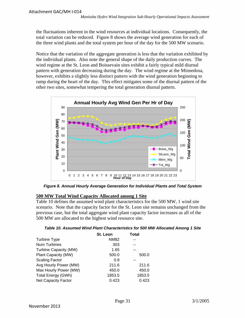
Manitoba Hydro Wind Integration Sub-Hourly Operational Impacts Assessment
the fluctuations inherent in the wind resources at individual locations. Consequently, the total variation can be reduced. Figure 8 shows the average wind generation for each of the three wind plants and the total system per hour of the day for the 500 MW scenario.
Notice that the variation of the aggregate generation is less that the variation exhibited by the individual plants. Also note the general shape of the daily production curves. The wind regime at the St. Leon and Boissevain sites exhibit a fairly typical mild diurnal pattern with generation decreasing during the day. The wind regime at the Minnedosa, however, exhibits a slightly less distinct pattern with the wind generation beginning to ramp during the heart of the day. This effect mitigates some of the diurnal pattern of the other two sites, somewhat tempering the total generation diurnal pattern.
Annual Hourly Avg Wind Gen Per Hr of Day
0
10
20
30
40
50
60
70
80
90
0 1 2 3 4 5 6 7 8 9 10 11 12 13 14 15 16 17 18 19 20 21 22 23Hour of Day
Pla
nt
Win
d G
en (
MW
)
0
50
100
150
200
250
To
tal W
ind
Gen
(M
W)
Boiss_Wg
StLeon_Wg
Minn_Wg
Tot_Wg
Figure 8. Annual Hourly Average Generation for Individual Plants and Total System
500 MW Total Wind Capacity Allocated among 1 Site Table 10 defines the assumed wind plant characteristics for the 500 MW, 1 wind site scenario. Note that the capacity factor for the St. Leon site remains unchanged from the previous case, but the total aggregate wind plant capacity factor increases as all of the 500 MW are allocated to the highest wind resource site.
Table 10. Assumed Wind Plant Characteristics for 500 MW Allocated Among 1 Site St. Leon Total
Turbine Type NM82 -- Num Turbines 303 -- Turbine Capacity (MW) 1.65 -- Plant Capacity (MW) 500.0 500.0Scaling Factor 0.9 -- Avg Hourly Power (MW) 211.6 211.6Max Hourly Power (MW) 450.0 450.0Total Energy (GWh) 1853.5 1853.5Net Capacity Factor 0.423 0.423
Page 31 3/1/2005
Attachment GAC/MH I-014
November 2013

Manitoba Hydro Wind Integration Sub-Hourly Operational Impacts Assessment
Figure 9 shows the April 2003 time series resulting from the wind generation synthesis process for the 500 MW wind plant allocated at a single site.
Apr 2003 Hourly Total Wind Generation (500 MW)
0.00
50.00
100.00
150.00
200.00
250.00
300.00
350.00
400.00
450.00
500.00
4/1/
2003
0:0
0
4/1/
03 2
3:00
4/2/
03 2
2:00
4/3/
03 2
1:00
4/4/
03 2
0:00
4/5/
03 1
9:00
4/6/
03 1
8:00
4/7/
03 1
7:00
4/8/
03 1
6:00
4/9/
03 1
5:00
4/10
/03
14:0
0
4/11
/03
13:0
0
4/12
/03
12:0
0
4/13
/03
11:0
0
4/14
/03
10:0
0
4/15
/03
9:00
4/16
/03
8:00
4/17
/03
7:00
4/18
/03
6:00
4/19
/03
5:00
4/20
/03
4:00
4/21
/03
3:00
4/22
/03
2:00
4/23
/03
1:00
4/24
/03
0:00
4/24
/03
23:0
0
4/25
/03
22:0
0
4/26
/03
21:0
0
4/27
/03
20:0
0
4/28
/03
19:0
0
4/29
/03
18:0
0
4/30
/03
17:0
0
Date
Win
d G
en (
MW
)
Figure 9. Hourly Total Wind Generation Time series for 500 MW, 1 Site Scenario
The average hourly wind production for the 500 MW one site scenario is shown in Figure 10. Note that this graphic indicates a seasonal output pattern where the wind productionis lowest in the summer months of June-August and highest in the winter and spring months. Note that the output for the month of January is significantly lower than the surrounding high output months of December and February. This is due in part to the cold weather operating limit of the turbines.
Monthly Variation of Average Hourly Wind Production
0
50
100
150
200
250
300
Apr-03
May-03
Jun-03
Jul-03 Aug-03
Sep-03
Oct-03
Nov-03
Dec-03
Jan-04
Feb-04
Mar-04
Win
d G
ener
atio
n (
MW
)
StLeon_Wg
Figure 10. 500 MW/3 Site Scenario -- Average Hourly Power Output per Month
Page 32 3/1/2005
Attachment GAC/MH I-014
November 2013

Manitoba Hydro Wind Integration Sub-Hourly Operational Impacts Assessment
4.1.5. Spatial Diversity Affect for 500 MW Scenarios It has already been shown from Figure 8 that allocation of the total wind plant among geographically diverse provides diversity in the fluctuations inherent in the wind resources at individual locations. Consequently, the total variation can be reduced. Figure 11 shows the hourly wind generation output for the month of April for the three allocation scenarios for the 500 MW wind capacity level and further emphasizes the beneficial affects of diversity. Note that the hourly output for the 1-site scenarios exhibits more extreme swings, with more occasions at both the peak output and zero output. It should be noted that the 3-site scenario shows less drastic changes in output and is often somewhere between the output curves for the 1- and 2-site scenarios. Also note that the “flat-lining” that occurs at the maximum plant output level of the single site allocation scenario is a result of the wind speed remaining above rated speed for several consecutive hours. Because the simplified synthesis model utilized assumes that all turbines with the plant see exactly the same wind speed for the entire hour, the output waveform exhibits this “flat-line” characteristic during periods of sustained high wind. In reality, there would likely be some variation in wind speed within the plant during the hour such that not all turbines would have exactly identical maximum output for the hour.
Apr 2003 Hourly Total Wind Generation (500 MW)
0.00
50.00
100.00
150.00
200.00
250.00
300.00
350.00
400.00
450.00
500.00
4/1/
2003
4/1/
03 2
3:00
4/2/
03 2
2:00
4/3/
03 2
1:00
4/4/
03 2
0:00
4/5/
03 1
9:00
4/6/
03 1
8:00
4/7/
03 1
7:00
4/8/
03 1
6:00
4/9/
03 1
5:00
4/10
/03
14:0
0
4/11
/03
13:0
0
4/12
/03
12:0
0
4/13
/03
11:0
0
4/14
/03
10:0
0
4/15
/03
9:00
4/16
/03
8:00
4/17
/03
7:00
4/18
/03
6:00
4/19
/03
5:00
4/20
/03
4:00
4/21
/03
3:00
4/22
/03
2:00
4/23
/03
1:00
4/24
/03
0:00
4/24
/03
23:0
0
4/25
/03
22:0
0
4/26
/03
21:0
0
4/27
/03
20:0
0
4/28
/03
19:0
0
4/29
/03
18:0
0
4/30
/03
17:0
0
Date
Win
d G
en (
MW
)
500MW_3Sites
500MW_2Sites
500MW_1Site
Figure 11. Comparison of hourly time series for 500 MW allocated among 1, 2, and 3 sites.
Figure 12 shows a comparison of the monthly average hourly output for each of the three allocation scenarios for the 500 MW total capacity level. Although it is more difficult to discern the spatial diversity affect when analyzing the monthly hourly average values, one can see that the change in output from month to month is less for the 2- and 3- site scenarios than for the single site scenario.
Page 33 3/1/2005
Attachment GAC/MH I-014
November 2013

Manitoba Hydro Wind Integration Sub-Hourly Operational Impacts Assessment
Monthly Variation of Average Hourly Wind Production
0
50
100
150
200
250
300
Apr-03
May-03
Jun-03
Jul-03 Aug-03
Sep-03
Oct-03
Nov-03
Dec-03
Jan-04
Feb-04
Mar-04
Win
d G
ener
atio
n (
MW
)500MW_3Sites
500MW_2Sites
500MW_1Site
Figure 12. Comparison of monthly average hourly output for 500 MW allocated among 1, 2, and 3 sites.
A more rigorous approach to analyzing the affect of spatial diversity involves constructing probability distributions for the changes in wind generation output for the various allocation scenarios. Figure 13, Figure 14, and Figure 15 show the relative and cumulative probability distributions of the hourly change in real power output for the 3 allocation scenarios for the 500 MW capacity level. The distributions definitely show that as the total wind plant is spread among an increasing number of spatially diverse sites, the degree of fluctuation decreases. This spatial diversity benefit is evident from both spread of the distribution and the extremities of the distributions as summarized in Table 11. Notice that the standard deviation of the distribution decreases from 56 MW for St. Leon in isolation to 36.5 MW when the 500 MW is allocated evenly among the 3 sites. Furthermore, the 5% and 95% cumulative probabilities and minimum and maximum distribution values, show similar spatial diversity benefits. For example, the data indicates that for a single site, the wind generation may drop as much as 370 MW from one hour to the next and more than 5% of the hourly changes will be decreases in output of more than 91 MW. When the 500 MW total capacity is spread among the 3 sites, the maximum hourly drop decreases to 223 MW (150 MW improvement) and the CP05 value to 60 MW (30 MW improvement). The other statistical values presented can be compared to obtain a similar trend. This analysis will be conducted for the higher resolution data when performing the regulation impact analysis.
Page 34 3/1/2005
Attachment GAC/MH I-014
November 2013

Manitoba Hydro Wind Integration Sub-Hourly Operational Impacts Assessment
Table 11. Summary of hourly real power fluctuations as total wind plant is spread among increasing number of spatially separated locations.
Allocation Scenario
Std Dev (MW)
CP05 (MW)
Max Neg. Change
(MW) CP95 (MW)
Max Pos. Change
(MW)
500 MW – 1 Site 55.97 -91.1 -370.0 92.3 373.4
500 MW – 2 Sites 39.92 -64.5 -272.3 67.0 231.9
500 MW – 3 Sites 36.52 -59.6 -222.9 62.2 224.4
0%
2%
4%
6%
8%
10%
12%
14%
16%
0%
10%
20%
30%
40%
50%
60%
70%
80%
90%
100%
-200 -100 0 100 200
Hourly Delta P - 500 MW for 3 SitesData for 4/1/03 - 4/1/04
Electrotek/EPRI PQView®
Count: 8759Min: -222.9Avg: -0.01973Max: 224.4Range: 447.2St Dev: 36.52CP 01: -94.61CP 05: -59.61CP 25: -19.73CP 50: 0CP 75: 18.15CP 95: 62.20CP 99: 98.89SI Range: 18.94
Re
lativ
e F
req
ue
ncy
Cu
mu
lative
Fre
qu
en
cy
Delta P All (MW)
Relative Frequency Cumulative Frequency
Figure 13. Relative and cumulative probability distribution of hourly changes in real power output for the 500 MW capacity allocated among 3 wind plants.
Page 35 3/1/2005
Attachment GAC/MH I-014
November 2013
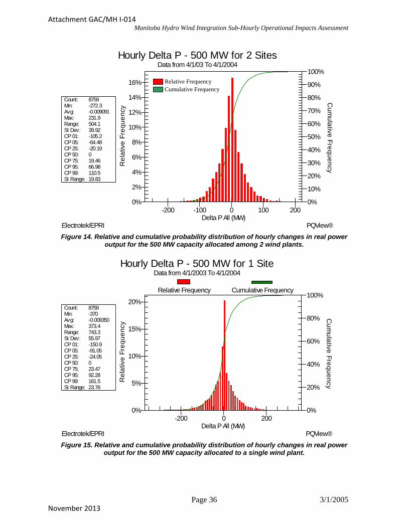
Manitoba Hydro Wind Integration Sub-Hourly Operational Impacts Assessment
0%
2%
4%
6%
8%
10%
12%
14%
16%
0%
10%
20%
30%
40%
50%
60%
70%
80%
90%
100%
-200 -100 0 100 200
Hourly Delta P - 500 MW for 2 SitesData from 4/1/03 To 4/1/2004
Electrotek/EPRI PQView®
Count: 8759Min: -272.3Avg: -0.009091Max: 231.9Range: 504.1St Dev: 39.92CP 01: -105.2CP 05: -64.48CP 25: -20.19CP 50: 0CP 75: 19.46CP 95: 66.98CP 99: 110.5SI Range: 19.83
Re
lativ
e F
req
ue
ncy
Cu
mu
lative
Fre
qu
en
cy
Delta P All (MW)
Relative Frequency Cumulative Frequency
Figure 14. Relative and cumulative probability distribution of hourly changes in real power output for the 500 MW capacity allocated among 2 wind plants.
0%
5%
10%
15%
20%
0%
20%
40%
60%
80%
100%
-200 0 200
Hourly Delta P - 500 MW for 1 SiteData from 4/1/2003 To 4/1/2004
Electrotek/EPRI PQView®
Count: 8759Min: -370Avg: -0.009350Max: 373.4Range: 743.3St Dev: 55.97CP 01: -150.9CP 05: -91.05CP 25: -24.05CP 50: 0CP 75: 23.47CP 95: 92.28CP 99: 161.5SI Range: 23.76
Re
lativ
e F
req
ue
ncy
Cu
mu
lative
Fre
qu
en
cy
Delta P All (MW)
Relative Frequency Cumulative Frequency
Figure 15. Relative and cumulative probability distribution of hourly changes in real power
output for the 500 MW capacity allocated to a single wind plant.
Page 36 3/1/2005
Attachment GAC/MH I-014
November 2013

Manitoba Hydro Wind Integration Sub-Hourly Operational Impacts Assessment
4.2 Interaction with System Load For the hourly scheduling simulations to be conducted by the other contractor, the wind generation time series will likely be subtracted from the year 2010 system load time series to yield a net load series as generation requirement to be met by the hydraulic generating resources and energy transactions. As noted previously, the projected Y2010 hourly system load series was calculated by MH personnel. The Y2010 average load per hour of the day is shown in Figure 16, along with the average hourly wind generation for the 500 MW, 3 site wind capacity scenario. Notice that the daily load shape exhibits a typical “day-peaking” characteristic with a ramp-up in early morning hours and ramp-down in the late evening hours. The average morning ramp occurs from approximately 4 a.m. to 8 a.m. with the average hourly ramping on the order of 100 – 150 MW per hour. The slight diurnal pattern of the wind generation, however, ramps in an almost inverted pattern to the load ramp. The values shown in Figure 16 are averages, and the actual ramping on any given hour varies depending on the season of the year. Figure 16 provides a general sense of this relationship by comparing the 500 MW scenario daily wind generation shape to the load shape. Note that the scale of the wind generation series is much smaller to allow for a sense of the shape of the curves.
Y2010 Avg. Hourly Load and Wind Gen
1500
1700
1900
2100
2300
2500
2700
2900
3100
0 2 4 6 8 10 12 14 16 18 20 22
Hr of Day
Lo
ad M
W
100
120
140
160
180
200
220
Win
d G
en M
WY2010_Ld
Tot_Wg
Figure 16. Y2010 Average Hourly Load Compared with 500 MW Scenario Wind Generation
4.3 Regulation Time Frame (1-minute resolution) The statistical analysis of the impacts of high-frequency wind generation fluctuations requires high-resolution system load and wind generation data. The regulation impact analysis is performed at a resolution of 1 minute to correlate with the highest resolution addressed by the NERC system performance standards CPS1 and CPS24. This subsection describes the models utilized for obtaining these data sets.
4 NERC Operating Manual Policy 1 – Generation Control and Performance, Version 1a, October 8, 2002, (available at ftp://www.nerc.com/pub/sys/all_updl/oc/opman/policy1_BOTApproved_1002.doc).
Page 37 3/1/2005
Attachment GAC/MH I-014
November 2013

Manitoba Hydro Wind Integration Sub-Hourly Operational Impacts Assessment
4.3.1. System Load Data Source As noted, the wind impact study is conducted for the expected MH Y2009/Y2010 system for which actual measured high-resolution load data does not exist. The regulation analysis approach, which is described in detail in a subsequent section, requires that the high-frequency fluctuation component of the load series be synthesized for the study year rather than the actual load series itself. This required data is synthesized from the following data sources:
MH 4-sec resolution load data from EMS archive for 1-year period of 4/1/03through 4/1/04 (Y2003/2004 load series)MH hourly resolution load series for study year ranging from 4/1/09 through4/1/04. Manitoba Hydro load forecasting personnel synthesized 100 possible loadseries for the study year. This process involved averaging various potential loadsituations in order to provide a “typical” load year for the forecast years beyond 2years in the future, which applies to our study year of Y2009/2010. From these100 load series, one 8760 series was selected by MH personnel as the Y2010 loadseries to be utilized for the study.
Data Quality Assurance and Augmentation (Filling Data Gaps) A 1-minute resolution system load series was calculated from the 4-second resolution Y2003/2004 load series by averaging based on clock minute intervals. This 1-minute Y2003/2004 series was then analyzed to determine the extent of data coverage (i.e., gaps within the data) with the results shown in Table 12. The coverage of the 1-minute data was found to be relatively high with only one significant gap in the data -- a gap of 7 days in late April 2003. There was one other data gap of approximately 30 minutes, with the remainder of the gaps being 1-3 minutes in duration as shown in the “Original Data” columns of Table 12. In analyzing the data gaps, it was found that the load value changed significantly across several of the identified data gaps (“Original Data – Load ∆” column of Table 12). MH personnel confirmed that these periods correlated to EMS data collection errors. As a result, “bad data points” immediately following the data gaps were deleted from the underlying 4-second resolution EMS data. This in effect increased the size of some of the gaps by a few minutes, with the resulting base data coverage analysis as shown in the “After Deletion” columns of Table 12.
It should be noted that after most of the analyses conducted in this study were completed, it was determined that at least 3 large probably load data errors still remained in the load data set – May 19, October 21, and January 21. The suspect data from these dates were not associated with a data gap or any MH EMS error known of at the time. As a result, these likely erroneous load data values were included in the subsequent impact analyses conducted. Due to the number of data points in the minute-to-minute load and net load change probability distributions, as well as the fact that these significant load changes impact both the base case load series and the with wind generation net load series, these three additional bad data events do not significantly impact the impact findings presented in this report.
Page 38 3/1/2005
Attachment GAC/MH I-014
November 2013

Manitoba Hydro Wind Integration Sub-Hourly Operational Impacts Assessment
Notice that Table 12 also states the method used to fill the data gaps. The preferred methods of filling the gaps in descending order of priority were as follows:
1. If data gap consists of 60 points or less (<=1hour), the data is replaced by astraight-line interpolation between the surrounding known points.
2. If data gap consists of more than 60 points (>1 hour), the gap is filled withcontiguous data points corresponding to the same clock period for days just priorto or just after the data gap. For example, data from 1/14/04 00:00 to 11/14/0417:50 is replaced with data from 1/13/04 00:00 to 11/13/04 17:50 if original dataexists without gaps.
Table 12. Data coverage analysis for MH high resolution load data from Y2003/2004.
# Miss. Load ∆ # Miss. Load ∆ Method for Replacing Begin Data Gap End Data Gap Pts. (MW) Pts. (MW) Missing Data
4/9/2003 2:24:00 PM 4/9/2003 2:24:00 PM 1 1520.9 4 4.3 Interpolation 4/20/2003 11:00:00 PM 4/27/2003 10:59:00 PM 10080 86.0 10080 86.0 Same time period from previous data
5/1/2003 2:15:00 PM 5/1/2003 2:16:00 PM 2 1284.0 9 74.1 Interpolation 5/8/2003 1:49:00 PM 5/8/2003 1:49:00 PM 1 -211.1 1 -211.1 Interpolation
5/15/2003 9:16:00 AM 5/15/2003 9:17:00 AM 2 2.7 2 2.7 Interpolation 5/29/2003 2:24:00 PM 5/29/2003 2:25:00 PM 2 616.3 3 12.3 Interpolation 6/23/2003 1:27:00 PM 6/23/2003 1:28:00 PM 2 -1.2 2 -1.2 Interpolation 6/23/2003 3:28:00 PM 6/23/2003 3:30:00 PM 3 0.8 3 0.8 Interpolation 7/3/2003 10:53:00 AM 7/3/2003 10:53:00 AM 1 784.0 2 -45.1 Interpolation 7/9/2003 10:47:00 AM 7/9/2003 10:47:00 AM 1 -15.2 1 -15.2 Interpolation 7/9/2003 12:21:00 PM 7/9/2003 12:21:00 PM 1 4.7 1 4.7 Interpolation 7/24/2003 1:20:00 PM 7/24/2003 1:22:00 PM 3 625.9 6 9.6 Interpolation 8/6/2003 2:13:00 PM 8/6/2003 2:13:00 PM 1 -26.8 1 -26.8 Interpolation 9/3/2003 1:43:00 PM 9/3/2003 1:43:00 PM 1 1194.8 2 -12.3 Interpolation 9/8/2003 3:43:00 PM 9/8/2003 3:43:00 PM 1 -1068.7 2 -55.6 Interpolation 9/9/2003 1:43:00 PM 9/9/2003 1:43:00 PM 1 0.8 1 0.8 Interpolation
9/16/2003 2:46:00 PM 9/16/2003 2:46:00 PM 1 256.1 1 256.1 Interpolation 10/2/2003 1:44:00 PM 10/2/2003 1:44:00 PM 1 1981.0 2 19.7 Interpolation
10/24/2003 10:02:00 AM 10/24/2003 10:02:00 AM 1 0.2 1 0.2 Interpolation 10/27/2003 9:47:00 AM 10/27/2003 10:15:00 AM 29 550.8 31 -2.1 Interpolation 11/4/2003 11:16:00 AM 11/4/2003 11:16:00 AM 1 -10.2 1 -10.2 Interpolation 11/6/2003 2:24:00 PM 11/6/2003 2:24:00 PM 1 1749.0 3 12.4 Interpolation
11/19/2003 11:25:00 AM 11/19/2003 11:25:00 AM 1 41.1 1 41.1 Interpolation 11/27/2003 1:21:00 PM 11/27/2003 1:21:00 PM 1 1283.8 2 -2.5 Interpolation 1/15/2004 2:37:00 PM 1/15/2004 2:37:00 PM 1 1587.6 34 42.7 Interpolation 2/5/2004 12:50:00 PM 2/5/2004 12:50:00 PM 1 361.5 2 13.4 Interpolation 2/12/2004 1:31:00 PM 2/12/2004 1:31:00 PM 1 5.9 1 5.9 Interpolation 2/18/2004 1:48:00 PM 2/18/2004 1:48:00 PM 1 -42.0 1 -42.0 Interpolation 3/11/2004 1:29:00 PM 3/11/2004 1:30:00 PM 2 -14.3 2 -14.3 Interpolation
3/22/2004 10:48:00 AM 3/22/2004 10:48:00 AM 1 -6.4 1.0 -6.4 Interpolation
Original Data After Deletion
Temporal Data Normalization The actual year for which the impact study is performed is the MH load year of 2009/2010, which spans 4/1/2009 through 3/31/2010. MH personnel calculated a projected load series for the study year based on a process conducted internally by MH personnel. This process entails averaging of various potential load situations and provides a “typical” load year for the forecast years beyond 2 years in the future, which applies to our study year of Y2009/2010. This “typical” forecast series consists of an
Page 39 3/1/2005
Attachment GAC/MH I-014
November 2013
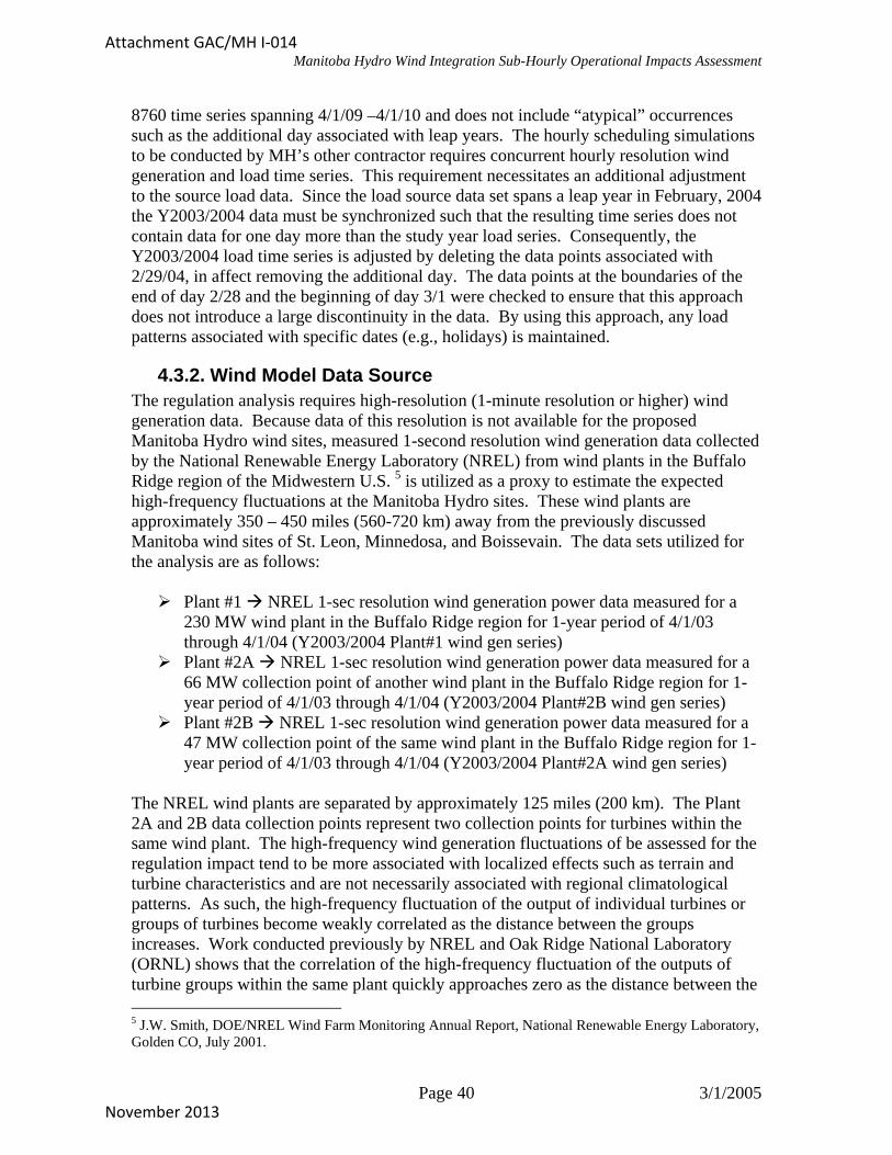
Manitoba Hydro Wind Integration Sub-Hourly Operational Impacts Assessment
8760 time series spanning 4/1/09 –4/1/10 and does not include “atypical” occurrences such as the additional day associated with leap years. The hourly scheduling simulations to be conducted by MH’s other contractor requires concurrent hourly resolution wind generation and load time series. This requirement necessitates an additional adjustment to the source load data. Since the load source data set spans a leap year in February, 2004 the Y2003/2004 data must be synchronized such that the resulting time series does not contain data for one day more than the study year load series. Consequently, the Y2003/2004 load time series is adjusted by deleting the data points associated with 2/29/04, in affect removing the additional day. The data points at the boundaries of the end of day 2/28 and the beginning of day 3/1 were checked to ensure that this approach does not introduce a large discontinuity in the data. By using this approach, any load patterns associated with specific dates (e.g., holidays) is maintained.
4.3.2. Wind Model Data Source The regulation analysis requires high-resolution (1-minute resolution or higher) wind generation data. Because data of this resolution is not available for the proposed Manitoba Hydro wind sites, measured 1-second resolution wind generation data collected by the National Renewable Energy Laboratory (NREL) from wind plants in the Buffalo Ridge region of the Midwestern U.S. 5 is utilized as a proxy to estimate the expected high-frequency fluctuations at the Manitoba Hydro sites. These wind plants are approximately 350 – 450 miles (560-720 km) away from the previously discussed Manitoba wind sites of St. Leon, Minnedosa, and Boissevain. The data sets utilized for the analysis are as follows:
Plant #1 NREL 1-sec resolution wind generation power data measured for a230 MW wind plant in the Buffalo Ridge region for 1-year period of 4/1/03through 4/1/04 (Y2003/2004 Plant#1 wind gen series)Plant #2A NREL 1-sec resolution wind generation power data measured for a66 MW collection point of another wind plant in the Buffalo Ridge region for 1-year period of 4/1/03 through 4/1/04 (Y2003/2004 Plant#2B wind gen series)Plant #2B NREL 1-sec resolution wind generation power data measured for a47 MW collection point of the same wind plant in the Buffalo Ridge region for 1-year period of 4/1/03 through 4/1/04 (Y2003/2004 Plant#2A wind gen series)
The NREL wind plants are separated by approximately 125 miles (200 km). The Plant 2A and 2B data collection points represent two collection points for turbines within the same wind plant. The high-frequency wind generation fluctuations of be assessed for the regulation impact tend to be more associated with localized effects such as terrain and turbine characteristics and are not necessarily associated with regional climatological patterns. As such, the high-frequency fluctuation of the output of individual turbines or groups of turbines become weakly correlated as the distance between the groups increases. Work conducted previously by NREL and Oak Ridge National Laboratory (ORNL) shows that the correlation of the high-frequency fluctuation of the outputs of turbine groups within the same plant quickly approaches zero as the distance between the
5 J.W. Smith, DOE/NREL Wind Farm Monitoring Annual Report, National Renewable Energy Laboratory, Golden CO, July 2001.
Page 40 3/1/2005
Attachment GAC/MH I-014
November 2013

Manitoba Hydro Wind Integration Sub-Hourly Operational Impacts Assessment
turbine groups increases6. Thus, the two separate collection points are utilized to represent two separate plants for the regulation impact assessment.
It would obviously be preferable to have actual high frequency data for the Manitoba sites such that the specific terrain effects, turbine characteristics, etc. would be reflected in the analysis. In the absence of site-specific, high-resolution data, however, utilizing the available NREL data is considered a reasonable approximation given the fact that the fluctuations of an entire wind plant are also strongly related to the plant capacity due to the spatial diversity benefits mentioned.
The three NREL data locations are mapped to the three Manitoba sites as follows:
St. Leon Plant #1 Minnedosa Plant #2B Boissevain Plant #2A
This mapping is based solely on the size of the existing wind plants and the allocations of projected wind capacity scenarios for the Manitoba sites. For example, because St. Leon is utilized as one of the two sites for the base case allocations and the only site for the spatial diversity 1-site scenarios, the NREL data for the largest wind plant is utilized.
Data Quality Assurance and Augmentation (Filling Data Gaps) A 1-minute resolution average wind generation time series were calculated from the 1-second resolution Y2003/2004 series for each of the three sites. These 1-minute Y2003/2004 series were then analyzed to determine the extent of data coverage (i.e., gaps within the data) with the results shown in Table 13, Table 14, and Table 15. The coverage of the 1-minute data was found to be relatively high with the Plant #1 data containing only one significant gap of 13 days in mid-February 2004 and the Plant #2 data sets containing two significant gaps of 14 and 18 days in early May 2003 and early February 2004, respectively. There were other data gaps of less than 30 minutes for each of the sites.
Notice that Table 13, Table 14, and Table 15 also state the method used to fill the data gaps. The preferred methods of filling the gaps in descending order of priority were as follows:
1. If data gap consists of 60 points or less (<=1hour), the data is replaced by astraight-line interpolation between the surrounding known points.
2. If data gap consists of more than 60 points (>1 hour), the gap is filled withcontiguous data points corresponding to the same clock period for days just priorto or just after the data gap. For example, data from 1/14/04 00:00 to 11/14/0417:50 is replaced with data from 1/13/04 00:00 to 11/13/04 17:50 if original dataexists without gaps.
6 Randy Hudson, Brendan Kirby, Yih-Huei Wan, “The Impact of Wind Generation on System Regulation Requirements,” AWEA WindPower 2001,Washington D.C., June, 2001.
Page 41 3/1/2005
Attachment GAC/MH I-014
November 2013

Manitoba Hydro Wind Integration Sub-Hourly Operational Impacts Assessment
Table 13. Data coverage analysis for Plant #1 (representing St. Leon) high-resolution wind generation data from Y2003/2004.
# Miss. Gen ∆ Method for Replacing Begin Data Gap End Data Gap Pts. (MW) Missing Data
4/1/2003 11:04:00 PM 4/1/2003 11:09:00 PM 6 2.5 Interpolation 5/2/2003 9:04:00 PM 5/2/2003 9:09:00 PM 6 0.1 Interpolation
11/24/2003 2:17:00 AM 11/24/2003 2:19:00 AM 3 -2.1 Interpolation
2/5/2004 12:10:00 AM 2/18/2004 12:09:00 AM 18720 -35.4Data from 1/5/04 to 1/18/04 with smoothing at boundaries
2/20/2004 6:08:00 AM 2/20/2004 6:15:00 AM 8 0.9 Interpolation 3/26/2004 10:59:00 PM 3/26/2004 10:59:00 PM 1 -0.5 Interpolation
Table 14. Data coverage analysis for Plant #2B (representing Minnedosa) high-resolution wind generation data from Y2003/2004.
# Miss. Gen ∆ Method for Replacing Begin Data Gap End Data Gap Pts. (MW) Missing Data
4/4/2003 9:04:00 AM 4/4/2003 9:09:00 AM 6 -1.4 Interpolation 4/4/2003 9:18:00 AM 4/4/2003 9:19:00 AM 2 -4.9 Interpolation
4/4/2003 10:07:00 AM 4/4/2003 10:09:00 AM 3 -2.3 Interpolation 4/4/2003 10:59:00 AM 4/4/2003 10:59:00 AM 1 1.4 Interpolation 4/4/2003 11:37:00 AM 4/4/2003 11:39:00 AM 3 -0.2 Interpolation 4/4/2003 12:27:00 PM 4/4/2003 12:29:00 PM 3 4.7 Interpolation 4/4/2003 12:34:00 PM 4/4/2003 12:39:00 PM 6 -1.6 Interpolation 4/4/2003 12:44:00 PM 4/4/2003 12:49:00 PM 6 1.7 Interpolation 4/4/2003 12:53:00 PM 4/4/2003 12:59:00 PM 7 -25.7 Interpolation 4/6/2003 9:49:00 AM 4/6/2003 9:49:00 AM 1 0.2 Interpolation
4/6/2003 10:19:00 AM 4/6/2003 10:19:00 AM 1 5.2 Interpolation 4/6/2003 11:27:00 AM 4/6/2003 11:29:00 AM 3 -0.3 Interpolation 4/9/2003 8:47:00 AM 4/9/2003 8:49:00 AM 3 0.1 Interpolation 4/9/2003 9:49:00 AM 4/9/2003 9:49:00 AM 1 0.3 Interpolation 4/9/2003 9:58:00 AM 4/9/2003 9:59:00 AM 2 0.8 Interpolation
4/20/2003 8:40:00 PM 4/20/2003 8:50:00 PM 11 0.2 Interpolation
4/30/2003 12:10:00 AM 5/14/2003 12:09:00 AM 20160 -18.9Data from 3/29/03 to 4/12/03 with smoothing at boundaries
6/14/2003 12:37:00 AM 6/14/2003 12:39:00 AM 3 -0.3 Interpolation 6/14/2003 5:07:00 AM 6/14/2003 5:09:00 AM 3 0.3 Interpolation 6/27/2003 8:23:00 PM 6/27/2003 8:29:00 PM 7 -2.8 Interpolation 7/15/2003 5:50:00 AM 7/15/2003 6:08:00 AM 19 0.3 Interpolation 7/17/2003 2:25:00 AM 7/17/2003 2:29:00 AM 5 -0.6 Interpolation 8/9/2003 3:08:00 PM 8/9/2003 3:09:00 PM 2 0.0 Interpolation
8/11/2003 6:50:00 PM 8/11/2003 6:53:00 PM 4 0.6 Interpolation 9/13/2003 3:27:00 AM 9/13/2003 3:29:00 AM 3 0.9 Interpolation
10/2/2003 11:20:00 AM 10/2/2003 11:38:00 AM 19 -2.7 Interpolation 11/8/2003 12:38:00 AM 11/8/2003 12:38:00 AM 1 0.1 Interpolation 12/6/2003 5:30:00 AM 12/6/2003 5:48:00 AM 19 0.4 Interpolation
12/10/2003 11:10:00 AM 12/10/2003 11:14:00 AM 5 -0.2 Interpolation 1/7/2004 9:30:00 PM 1/7/2004 9:41:00 PM 12 6.6 Interpolation
1/31/2004 8:53:00 AM 2/18/2004 12:09:00 AM 25397 14.5Data from 1/26/04 to 1/8/04 with smoothing at boundaries
3/5/2004 8:29:00 PM 3/5/2004 8:29:00 PM 1 0.4 Interpolation 3/5/2004 8:36:00 PM 3/5/2004 8:39:00 PM 4 -1.7 Interpolation 3/5/2004 9:29:00 PM 3/5/2004 9:29:00 PM 1 -0.1 Interpolation
Page 42 3/1/2005
Attachment GAC/MH I-014
November 2013

Manitoba Hydro Wind Integration Sub-Hourly Operational Impacts Assessment
Table 15. Data coverage analysis for Plant #2A (representing Boissevain) high-resolution wind generation data from Y2003/2004.
# Miss. Gen ∆ Method for Replacing Begin Data Gap End Data Gap Pts. (MW) Missing Data
4/4/2003 10:37:00 AM 4/4/2003 10:39:00 AM 3 0.3 Interpolation 4/7/2003 5:50:00 AM 4/7/2003 5:51:00 AM 2 0.7 Interpolation
4/26/2003 1:54:00 PM 4/26/2003 1:54:00 PM 1 0.1 Interpolation
4/30/2003 12:10:00 AM 5/14/2003 12:09:00 AM 20160 -15.4Data from 3/29/03 to 4/12/03 with smoothing at boundaries
6/14/2003 1:08:00 AM 6/14/2003 1:09:00 AM 2 -0.4 Interpolation 6/14/2003 7:34:00 AM 6/14/2003 7:39:00 AM 6 0.8 Interpolation
6/14/2003 10:24:00 AM 6/14/2003 10:29:00 AM 6 -0.3 Interpolation 6/23/2003 8:54:00 AM 6/23/2003 8:59:00 AM 6 -0.7 Interpolation 7/5/2003 8:20:00 AM 7/5/2003 8:28:00 AM 9 1.5 Interpolation 7/8/2003 8:40:00 AM 7/8/2003 8:49:00 AM 10 1.2 Interpolation
8/5/2003 11:39:00 AM 8/5/2003 11:39:00 AM 1 0.1 Interpolation 8/19/2003 1:59:00 AM 8/19/2003 1:59:00 AM 1 0.4 Interpolation
8/22/2003 10:13:00 PM 8/22/2003 10:19:00 PM 7 -0.6 Interpolation 9/3/2003 11:00:00 PM 9/3/2003 11:18:00 PM 19 0.7 Interpolation
9/11/2003 11:20:00 AM 9/11/2003 11:28:00 AM 9 0.0 Interpolation 10/1/2003 5:40:00 AM 10/1/2003 5:58:00 AM 19 1.3 Interpolation
10/21/2003 11:00:00 AM 10/21/2003 11:10:00 AM 11 0.5 Interpolation 11/23/2003 6:40:00 AM 11/23/2003 6:58:00 AM 19 6.2 Interpolation 12/7/2003 5:00:00 AM 12/7/2003 5:18:00 AM 19 2.4 Interpolation
12/12/2003 3:00:00 PM 12/12/2003 3:10:00 PM 11 0.8 Interpolation 12/23/2003 3:25:00 PM 12/23/2003 3:25:00 PM 1 0.0 Interpolation
12/24/2003 10:45:00 PM 12/24/2003 10:46:00 PM 2 0.0 Interpolation 12/25/2003 11:00:00 PM 12/25/2003 11:11:00 PM 12 0.1 Interpolation 12/31/2003 6:53:00 AM 12/31/2003 6:59:00 AM 7 -1.1 Interpolation
1/1/2004 5:00:00 AM 1/1/2004 5:02:00 AM 3 -0.5 Interpolation 1/28/2004 11:45:00 PM 1/28/2004 11:49:00 PM 5 -0.8 Interpolation
1/31/2004 8:53:00 AM 2/18/2004 12:09:00 AM 25397 17.3Data from 1/25/04 to 1/7/04 with smoothing at boundaries
3/13/2004 2:50:00 PM 3/13/2004 3:08:00 PM 19 -0.1 Interpolation
Page 43 3/1/2005
Attachment GAC/MH I-014
November 2013

Manitoba Hydro Wind Integration Sub-Hourly Operational Impacts Assessment
5. Evaluation of the Impacts of Integrating Bulk Wind intothe Power Grid
5.1 High-Frequency Regulation Impact Assessment
5.1.1. General Approach Regulation is the process of deploying the control area’s fast-responding generating units to maintain the balance between demand (i.e., system load plus scheduled interchange) and supply (i.e., generation). In measuring how a particular control area balances the supply and demand, the North American Electric Reliability Council (NERC), through extensive research, has formulated two control performance standards (CPS) referred to as CPS1 and CPS27. Control areas within NERC’s jurisdiction are required to comply with the performance standards. Both CPS1 and CPS2 are defined based on the area control error (ACE), which is a metric of the difference between the area generation requirement and actual area generation for the control area. CPS1 and CPS2 measure the extent to which ACE is regulated within the associated control area. CPS1 is calculated using the 1-minute average ACE over a 12-month period. CPS2 is calculated using 10-minute average ACE over an entire calendar month. The minute-level resolution of the ACE values that are the basis of the NERC performance standard calculations implies that required time scale of deployment of control area generation to meet generation requirements is only at the minute level and not the sub-minute level. This is consistent with the response rates of fast responding thermal units.
High-frequency regulating reserve allocated to the fast responding units is deployed by automatic generation control (AGC) to compensate for the minute-to-minute variations of load through the regulation of ACE. Manitoba Hydro utilizes its hydro units at the Grand Rapids Hydro Station along the Saskatchewan River on AGC control for providing system regulation. Manitoba typically carries 40 - 50 MW of spinning regulating reserve in the up and down directions at Grand Rapids. Variability of system load governs the required amount of regulating reserve to meet the control performance standards. It is our experience that most North American utilities have developed regulating reserve requirements based on experiential analysis of CPS compliance. Researchers at the Oak Ridge National Lab (ORNL) developed a mathematical approach for determining the appropriate amount for regulating reserve8 based on the decomposition of the high-resolution time series into the summation of two components of different time scales:
• High frequency fluctuation time series, consistent with the total rampingcapabilities of generating units under AGC
• Slow and smooth variation time series, which is a moving average of the originaltime series with moving window size on the order of 30 to 60 minutes. Note thatthe width of moving average window is selected to appropriated allocated thefluctuations between regulation and load following components. As the length of
7 NERC Operating Manual Policy 1 – Generation Control and Performance, Version 1a, October 8, 2002. 8 Hudson, Kirby, and Wan, June, 2001.
Page 44 3/1/2005
Attachment GAC/MH I-014
November 2013

Manitoba Hydro Wind Integration Sub-Hourly Operational Impacts Assessment
the moving average window increases, more of the total fluctuation is attributed to regulation and less to load following, and vice versa.
A graphical example of these decomposed components is shown in Figure 17 for a single day of Manitoba Hydro load data. In Figure 17, the blue curve exhibiting a high degree of fluctuation around the daily load cycle is the actual high-resolution system load time series. The smooth green curve that follows the daily load cycle is the moving average of the original time series and is sometimes referred to as the “load-following” component of the system load. This component results from the slower varying portions of different individual loads, which are highly correlated. The highly volatile red curve is the high-frequency fluctuation component of the decomposition and is often referred to as the “regulation” component of the system load. The regulation component represents the uncorrelated, high frequency fluctuation of different individual loads within the system. This component is determined as the difference between the original high-resolution time series and the moving average. Because these high-frequency fluctuations are by definition statistically uncorrelated, the magnitude of this component grows proportional to the square root of the magnitude of the system load. The distribution of the regulation component is zero mean with a relatively small magnitude.
As noted in section 2.2, Manitoba Hydro is an indirect participant in deregulated electricity markets, and operates in a manner such that they carry spinning reserve for both the high-frequency “regulation” component and some portion of the “load-following” component, as those components are identified as resulting from the decomposition described here. MH actually allocates a total regulating reserve quantity, which comprises the spinning reserve to track the high-frequency variations (“regulation” as defined here), additional spinning reserve to follow sub-hourly load trends (a component of the “load following” as defined here), and non-spinning reserve that is withheld from market transactions for following the slower ramping of system load through the daily load cycle (the remainder of the “load following” as defined here).
The amount of high-frequency regulating reserve that must be carried to maintain system performance is related to being able to cover the high frequency fluctuation of the system load as described above. The ORNL method utilizes the standard deviation of the distribution comprising the high frequency fluctuation time series as a measure of the degree of fluctuation for determining regulating reserve requirement. The ORNL method hypothesizes that the appropriate amount of high-frequency regulating reserve that should be carried to maintain acceptable CPS performance is 3 times the high-frequency fluctuation standard deviation. This 3 standard deviation value was selected simply based on the fact that allocating reserve to cover 3 standard deviations of a normally distributed fluctuation distribution equates to a 99.73% confidence level of covering the these fluctuations. It should be noted that this allocation method is not necessarily utilized by utilities in determining regulating reserve requirements. As noted previously, the methods often used by utilities for this process are much more experiential than analytical. Nonetheless, the 3 standard deviation estimate provides a useful metric for benchmarking regulation requirements.
Page 45 3/1/2005
Attachment GAC/MH I-014
November 2013

Manitoba Hydro Wind Integration Sub-Hourly Operational Impacts Assessment
Decomposition of High-Freq Load Fluctuation
1900
2000
2100
2200
2300
2400
2500
2600
2700
-400
-300
-200
-100
0
100
200
300
400
Y2004_1-Min_LoadAvg
Y2004_30-Min_LoadMovAvg
Y2004_1-Min_LoadFluct
Figure 17. Decomposition into high-frequency and low frequency components for determination of regulation requirement.
5.1.2. Specific MH Assessment Method The historical high-resolution data available for the regulation impact analysis was processed as detailed in section 4.3.1 and 4.3.2. This data then had to be altered to represent the future study year and specific wind capacity scenarios. Note that the high-frequency fluctuation series is obtained via the ORNL decomposition method discussed previously with a moving average window of 30 minutes. The 30-minute value has been found to yield a high-frequency fluctuation series that is zero energy series corresponding to the regulation service in many de-regulated markets. The method utilized to scale the high-frequency fluctuation component of system load for the future study year is based on the assumption that fluctuations between individual loads are uncorrelated. Thus, the standard deviation of the future year fluctuation distribution is obtained by scaling the base case year fluctuation series by the square root of ratio of the future year hourly average load and reference year hourly average load. In actuality, there may be some slight positive correlation of the high frequency component, but the correlation is small.9 The result of assuming zero correlation is that the impact of wind generation on the high-frequency regulating reserve requirement will be slightly higher than if some small amount of positive correlation of system load were included. The slightly conservative impact of this assumption is considered minimal, however.
9 B. Kirby and E. Hirst, Customer-Specific Metrics for the Regulation and Load-Following Ancillary Services, ORNL/CON-474, Oak Ridge National Laboratory, January 2000.
Page 46 3/1/2005
Attachment GAC/MH I-014
November 2013
Manitoba Hydro Wind Integration Sub-Hourly Operational Impacts Assessment
The following steps describe the procedure of processing the 1-minute resolution system load data of year 2003/2004 (data resulting from processing described in section 4.3.1).
1. Calculate the 30-minute moving average time series for the base 1-minute resolution time series. The resulting moving average time series is also a 1-minute resolution series with the value of a given time point, t, calculated as the average of values of the base 1-minute resolution time series that fall within the window of t-15 minutes to t+15 minutes.
2. Calculate the high-frequency fluctuation time series by subtracting the original 1-minute resolution time series by the moving average time series.
3. It is assumed that the regulation component of system load is statistically uncorrelated. As such, this high-frequency component of the total system load scales according to the square root of the ratio of total system load for the new and base case scenarios. Thus, for the regulation analysis, each data point of the Y2003/Y2004 load high-frequency fluctuation series is scaled by the square root of the ratio of the corresponding hourly average load values for Y2009/2010 and Y2003//2004 as shown in Equation 3.
i
i
HR
HRii L
LLfLf
04/2003
10/200904/200310/2009 ×= Equation 3
where,
Lfi ≡ load fluctuation for 1-min resolution point i LHRi ≡ hourly average load corresponding to clock hour of 1-min resolution
fluctuation point i Figure 18 shows a trend of the resulting load multipliers (square root term of above equation) calculated from the specified approach. Note that although the majority of multipliers represent load growth from the base year to the study year, almost 20% of the hourly ratios indicate a reduction in load. Figure 19 shows the average value of the multipliers per hour of the day for all weekdays and weekend days. Notice that the multipliers are higher for the weekend days. It’s not clear if this is an expected result from the hourly load forecasting method used by MH personnel to produce the Y2009/2010 hourly load series. Nonetheless, the fact is noted here for later reference when analyzing the high-frequency regulation impact results.
Page 47 3/1/2005
Attachment GAC/MH I-014
November 2013

Manitoba Hydro Wind Integration Sub-Hourly Operational Impacts Assessment
Y2009/2010 High-Res Load Fluctuation Series Multiplier
0
0.2
0.4
0.6
0.8
1
1.2
1.4
Figure 18. Plot of load fluctuation series multipliers used to obtain Y2009/2010 high-resolution fluctuation series.
Hi-Res Load Fluctuation Avg Multiplier per Hour of Day
0.9
0.95
1
1.05
1.1
1.15
0 3 6 9 12 15 18 21 24
Hr of Day
Weekday
Weekend
Figure 19. Comparison of average load fluctuation series multipliers for weekdays and weekend days per hour of day.
Page 48 3/1/2005
Attachment GAC/MH I-014
November 2013

Manitoba Hydro Wind Integration Sub-Hourly Operational Impacts Assessment
The addition of wind generation into the Manitoba Hydro system changes the variability of net load (the system load net of the wind generation) relative to the variability of the load alone. Since the fluctuation of the system net load is the quantity that must be regulated to maintain the required system performance standard levels, the regulating reserve requirement changes when wind generation is added. The purpose of the regulation impact assessment is to determine the magnitude of this change in regulating reserve required.
As noted in section 4.3.2, there is no historical high-resolution wind generation or wind speed measurement data for the proposed Manitoba wind sites. As such, actual wind power data collected by NREL from wind power plants in the Buffalo Ridge region is used as a surrogate. As with the load data, this data was checked for quality and altered to obtain a full year of 1-minute resolution data for three wind plants. This base data set is then used to extract the minute-by-minute high-frequency fluctuation of wind generation from the original based high-resolution data set using a procedure similar to that described for the load. The distribution of these fluctuation series and associated standard deviation are then determined. As with the high-resolution load data, this source wind generation fluctuation distribution must be altered to reflect the desired study year scenarios. Unlike the load data, however, we do not assume any growth pattern for the wind resource. Rather, the study year scenarios to be analyzed require that we obtain high-resolution fluctuation series for each of the Manitoba sites for several different wind plant capacity levels that differ from the capacity levels represented by the source data measurements. Thus, for each of the wind plant capacity scenarios, the source data fluctuation series must be scaled to represent the desired scenario capacity allocations. Other studies have shown that the correlation of high-resolution fluctuations of the real power output of spatially separated wind turbine generators decreases as the distance between the turbines increases10,11. As a result, when scaling high-resolution fluctuations in wind plant output for an existing wind plant to represent the fluctuations for a non-existing plant of a different rated capacity, many studies have utilized the assumption that the high-frequency fluctuations for additional turbines within the same plant are statistically uncorrelated12,13. As such, the model utilized to obtain the wind generation fluctuation series for the various capacity allocations is as follows:
It is assumed that the regulation component of wind generation output is statistically uncorrelated. As such, this high-frequency component of the total wind generation output for a given capacity level scales according to the square root of the ratio of total capacity for the new and base case scenarios. Thus, for the regulation analysis, each data point of the Y2003/Y2004 wind generation high-frequency fluctuation series for any one of the 3 sites is scaled by the square
10 Hudson, Kirby, Wan, 2001. 11 Bernhard Ernst, Short-Term Power Fluctuations of Wind Turbines from the Ancillary Services Viewpoint, NREL/ISET, July 1999. 12 E. Hirst, Integrating Wind Energy with the BPA Power System: Preliminary Study, September 2002. 13 Daniel L. Brooks and Edward O. Lo, “Quantifying System Operation Impacts of Integrating Bulk Wind Generation at We Energies.” Proceedings of POWER-GEN Renewable Energy 2004, March 2004, Las Vegas, Nevada.
Page 49 3/1/2005
Attachment GAC/MH I-014
November 2013
Manitoba Hydro Wind Integration Sub-Hourly Operational Impacts Assessment
root of the ratio of the desired wind plant capacity and the source data capacity value as shown in Equation 4.
base
newii Wcap
WcapbaseWfnewWf ×−=− Equation 4
where,
Wfi ≡ wind generation fluctuation for 1-min resolution point i Wcap ≡ total wind plant capacity for scenario or measurement series
The assumption of zero correlation of the high-frequency fluctuations between turbines within the same plant is not exactly correct, as there is some non-zero, positive correlation between turbines separated by shorter distances within the plant. As such, scaling the high-frequency fluctuation standard deviation by the square root of the capacity ratio can slightly underestimate the magnitude of high-frequency fluctuations of the projected wind plant. In order to assess the potential underestimation resulting from this assumption, sensitivity analysis was conducted to determine the affect on total impacts of varying the scaling factor utilized. These results are summarized in the following Results and Analysis section.
Once the standard deviations of the system load and wind generation for a given study year capacity scenario are obtained from the procedures above, the standard deviation of the net system load is obtained by further assuming that high-frequency fluctuations of load and wind generation are uncorrelated. Under this assumption, the standard deviation of the aggregate fluctuation of wind and load is calculated as the square root of the sum of the squares of standard deviations of load and wind generation as shown in Equation 5.
22WindLoadNetLoad σσσ += Equation 5
where,
σNetLoad ≡ standard deviation of aggregate load and wind fluctuation σLoad ≡ standard deviation of load fluctuation σWind ≡ standard deviation of wind fluctuation
The standard deviation of the aggregate fluctuation is then used to determine the relative increase in high-frequency fluctuation resulting from integrating the various wind scenarios. This impact is calculated as the percent increase of the aggregate standard deviation over the standard deviation for the load alone (no wind generation scenario). Note that the percent increase in the standard deviation is the same as the percent increase in the ORNL regulation requirement (3 standard deviations). For the Manitoba study, we will use the percent increase in the high-frequency regulating reserve required to estimate the additional fast-responding reserve that must be provided by the Grand Rapid Station
Page 50 3/1/2005
Attachment GAC/MH I-014
November 2013

Manitoba Hydro Wind Integration Sub-Hourly Operational Impacts Assessment
for supporting wind generation integration. Note that this assessment does not consider additional reserve that might be carried at Grand Rapids for load following.
5.1.3. Results and Analysis Prior to analyzing the study year high-frequency regulation requirements, the high-frequency regulation burden for the existing system as indicated by the base year load data (4/1/03 – 4/1/04) is quantified in terms of the approach detailed above for comparison to Manitoba’s current operational practices. Figure 20 shows the relative and cumulative probability distributions for the Manitoba Y2003/2004 1-minute load changes. Note that this distribution is not the high-frequency fluctuation distribution, but simply the distribution of the changes in average system load from one minute to the next. This distribution provides a sense of the probability of regulation rates or ramping speeds required to meet the load changes from minute to minute. Note that the standard deviation of the 1-minute changes is approximately 10 MW, with the 5th and 95th cumulative probability values of –18.4 MW and 16.7 MW, respectively. This would indicate that a regulation down ramping rate of 18.4 MW/minute would cover all but 5% of one-minute load drops. Likewise, a regulation up ramping rate of 16.7 MW/minute would cover all but 5% of the 1-minute load increases. The large maximum and minimum values shown in the data block are additional bad data points that were identified after the analyses were completed. Three additional large load changes that were not associated with data gaps or the known MH EMS failures that were discussed in section 4.3.1 were recently verified as likely bad data. Due to the number of data points in the minute-to-minute load and net load change probability distributions, as well as the fact that these significant load changes impact both the base case load series and the with wind generation net load series, these three additional bad data events do not impact the analysis presented in this report. The maximum and minimum values shown in Figure 20, as well as Figure 21 and Figure 22, are likely an artifact of bad load data.
Page 51 3/1/2005
Attachment GAC/MH I-014
November 2013

Manitoba Hydro Wind Integration Sub-Hourly Operational Impacts Assessment
0%
5%
10%
15%
20%
25%
30%
35%
40%
0%
20%
40%
60%
80%
100%
-200 -100 0 100 200
Load Y2003/2004 1-Min Delta DistributionFrom 4/1/2003 To 4/1/2004
Electrotek/EPRI PQView®
Count: 527039Min: -479Avg: -0.0001484Max: 431.5Range: 910.4St Dev: 10.18CP 01: -31.25CP 05: -18.43CP 25: -3.753CP 50: 0.1999CP 75: 4.207CP 95: 16.71CP 99: 27.94SI Range:3.980
Rel
ativ
e F
requ
ency
Cum
ulative Frequency
Delta P All (MW)
Relative Frequency Cumulative Frequency
Figure 20. Distribution of Y2003/2004 minute-to-minute changes in Manitoba system load.
Figure 21 shows the relative and cumulative probability distributions of the Y2003/2004 high-frequency load fluctuations as determined by the ORNL decomposition method. This distribution shows that the standard deviation of the 1-minute fluctuations around the slower moving (30-min moving average), correlated component of the load is 15.19 MW. This is an interesting result in that the ORNL method for determining the high-frequency regulating reserve requirement to cover these fluctuations is three times the standard deviation or approximately 45.6 MW for the Y2003/2004 Manitoba system load. According to Manitoba personnel, approximately 40-50 MW of regulating reserve is typically carried at Grand Rapids for tracking these high-frequency fluctuations, as well as for providing some intra-hour load following. Thus, the 3 standard deviation approach appears to provide a reasonable approximation of Manitoba’s current operating practice. The statistical characteristics of the distribution are summarized in Table 16 along with the characteristics of the other relevant distributions analyzed as part of the high-frequency regulation impact assessment.
Although not the primary focus of the current project, the total Manitoba 1-minute load fluctuation distribution was analyzed further to gain additional insight into the potential for more efficient scheduling of the high-frequency regulating reserve. The distribution of 1-minute load fluctuations shown in Figure 21 was segregated into separate distributions for weekdays and weekend days. As expected, the magnitude of fluctuations on the weekend is less than on weekdays as the magnitude of the load itself is higher. The difference in the standard deviations is approximately 1.3 MW (see Table 16), which based on the 3 standard deviation approach suggests that Manitoba should carry on average 4 MW less high-frequency regulating reserve on weekends than on
Page 52 3/1/2005
Attachment GAC/MH I-014
November 2013

Manitoba Hydro Wind Integration Sub-Hourly Operational Impacts Assessment
weekdays. This difference would obviously decrease or increase for varying seasons as well.
0%
5%
10%
15%
20%
25%
30%
0%
20%
40%
60%
80%
100%
-200 -100 0 100 200
Load Y2003/2004 1-Min Fluctuation DistributionFrom 4/1/2003 To 4/1/2004
Electrotek/EPRI PQView®
Count: 527040Min: -818.7Avg: 0.00006116Max: 775.7Range: 1594St Dev: 15.19CP 01: -36.34CP 05: -26.93CP 25: -8.080CP 50: 1.963CP 75: 9.857CP 95: 20.48CP 99: 29.22SI Range:8.968
Rel
ativ
e F
requ
ency
Cum
ulative Frequency
P All (MW)
Relative Frequency Cumulative Frequency
Figure 21. Distribution of Y2003/2004 high-frequency load fluctuations as determined by ORNL decomposition method.
Table 16. Summary of probability distribution characteristics for various load and wind generation quantities. (Note all values are in units of MW.)
Distribution Quantity Min Max CP05 CP95 Std DevY03/04 1Min Load Delta -479 431.5 -18.43 16.71 10.18Fluctuation around 30-Min Moving Avg. Y03/04 1Min Load Fluct -818.7 775.7 -26.93 20.48 15.19 Weekdays -818.7 775.7 -26.99 20.92 15.56 Weekends -148 88.29 -26.78 19.45 14.24 Y09/10 1Min Load Fluct -658.7 624 -28.18 21.37 15.63 Weekdays -658.7 624 -27.88 21.30 15.67 Weekends -176.1 85.62 -28.87 21.54 15.55Fluctuation around 30-Min Moving Avg. Y03/04 1Min Plant #1 Wg Fluct -84.2 78.2 -3.55 3.70 3.04 Y03/04 1Min Plant #2A Wg Fluct -30.3 28.6 -1.18 1.20 0.93 Y03/04 1Min Plant #2B Wg Fluct -43.1 39.2 -1.80 1.85 1.40
Although the analysis of the Y2003/2004 load fluctuation series provides useful insights and confidence in the approach, the Y2009/2010 load fluctuation series is actually required for the study assessment. The Y2009/2010 1-minute load fluctuation series was developed as detailed previously from the Y2003/2004 series and the Y2009/2010 Manitoba estimate of hourly average load. The relative and cumulative probability distributions of the resulting Y2009/2010 fluctuation series are shown in Figure 22. The
Page 53 3/1/2005
Attachment GAC/MH I-014
November 2013
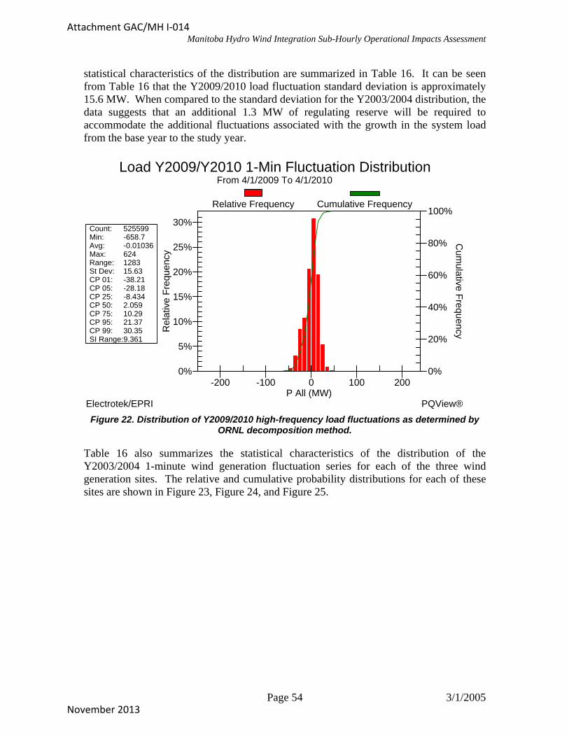
Manitoba Hydro Wind Integration Sub-Hourly Operational Impacts Assessment
statistical characteristics of the distribution are summarized in Table 16. It can be seen from Table 16 that the Y2009/2010 load fluctuation standard deviation is approximately 15.6 MW. When compared to the standard deviation for the Y2003/2004 distribution, the data suggests that an additional 1.3 MW of regulating reserve will be required to accommodate the additional fluctuations associated with the growth in the system load from the base year to the study year.
0%
5%
10%
15%
20%
25%
30%
0%
20%
40%
60%
80%
100%
-200 -100 0 100 200
Load Y2009/Y2010 1-Min Fluctuation DistributionFrom 4/1/2009 To 4/1/2010
Electrotek/EPRI PQView®
Count: 525599Min: -658.7Avg: -0.01036Max: 624Range: 1283St Dev: 15.63CP 01: -38.21CP 05: -28.18CP 25: -8.434CP 50: 2.059CP 75: 10.29CP 95: 21.37CP 99: 30.35SI Range:9.361
Rel
ativ
e F
requ
ency
Cum
ulative Frequency
P All (MW)
Relative Frequency Cumulative Frequency
Figure 22. Distribution of Y2009/2010 high-frequency load fluctuations as determined by ORNL decomposition method.
Table 16 also summarizes the statistical characteristics of the distribution of the Y2003/2004 1-minute wind generation fluctuation series for each of the three wind generation sites. The relative and cumulative probability distributions for each of these sites are shown in Figure 23, Figure 24, and Figure 25.
Page 54 3/1/2005
Attachment GAC/MH I-014
November 2013
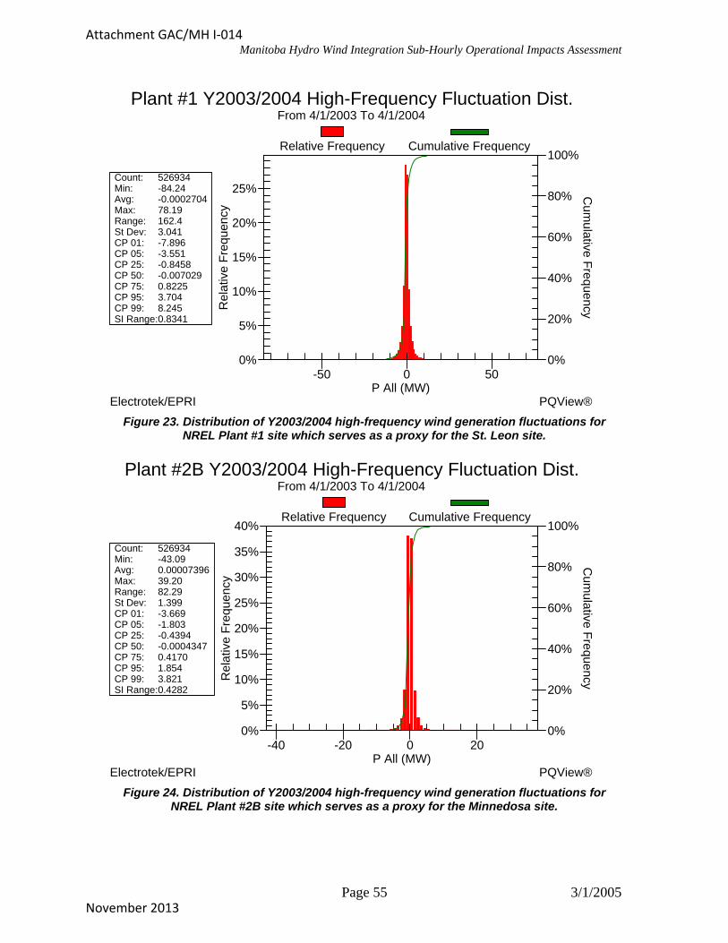
Manitoba Hydro Wind Integration Sub-Hourly Operational Impacts Assessment
0%
5%
10%
15%
20%
25%
0%
20%
40%
60%
80%
100%
-50 0 50
Plant #1 Y2003/2004 High-Frequency Fluctuation Dist.From 4/1/2003 To 4/1/2004
Electrotek/EPRI PQView®
Count: 526934Min: -84.24Avg: -0.0002704Max: 78.19Range: 162.4St Dev: 3.041CP 01: -7.896CP 05: -3.551CP 25: -0.8458CP 50: -0.007029CP 75: 0.8225CP 95: 3.704CP 99: 8.245SI Range:0.8341
Rel
ativ
e F
requ
ency
Cum
ulative Frequency
P All (MW)
Relative Frequency Cumulative Frequency
Figure 23. Distribution of Y2003/2004 high-frequency wind generation fluctuations for NREL Plant #1 site which serves as a proxy for the St. Leon site.
0%
5%
10%
15%
20%
25%
30%
35%
40%
0%
20%
40%
60%
80%
100%
-40 -20 0 20
Plant #2B Y2003/2004 High-Frequency Fluctuation Dist.From 4/1/2003 To 4/1/2004
Electrotek/EPRI PQView®
Count: 526934Min: -43.09Avg: 0.00007396Max: 39.20Range: 82.29St Dev: 1.399CP 01: -3.669CP 05: -1.803CP 25: -0.4394CP 50: -0.0004347CP 75: 0.4170CP 95: 1.854CP 99: 3.821SI Range:0.4282
Rel
ativ
e F
requ
ency
Cum
ulative Frequency
P All (MW)
Relative Frequency Cumulative Frequency
Figure 24. Distribution of Y2003/2004 high-frequency wind generation fluctuations for NREL Plant #2B site which serves as a proxy for the Minnedosa site.
Page 55 3/1/2005
Attachment GAC/MH I-014
November 2013
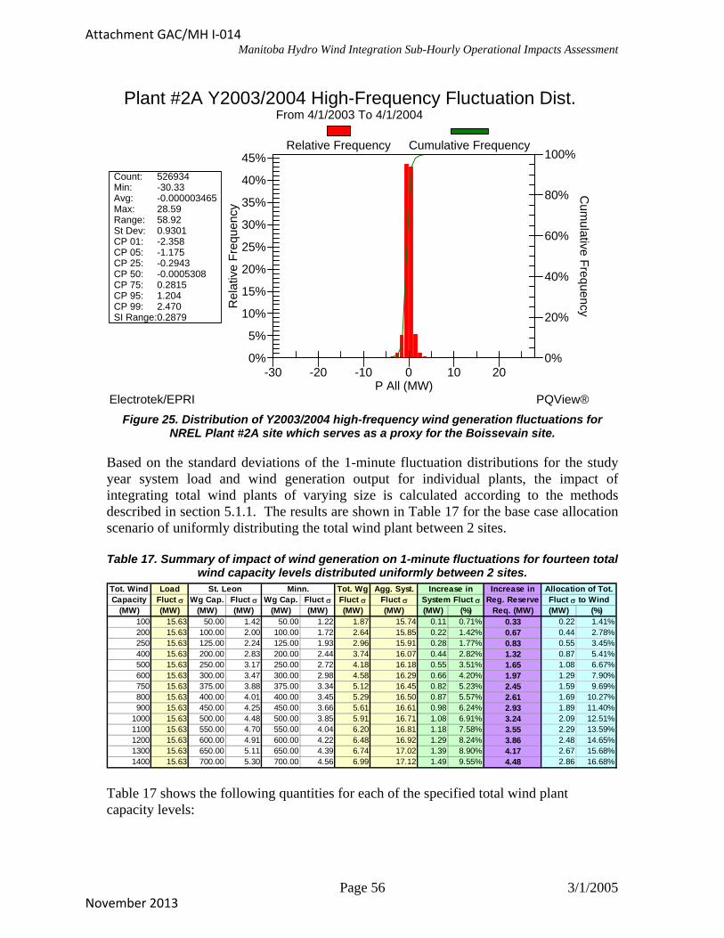
Manitoba Hydro Wind Integration Sub-Hourly Operational Impacts Assessment
0%
5%
10%
15%
20%
25%
30%
35%
40%
45%
0%
20%
40%
60%
80%
100%
-30 -20 -10 0 10 20
Plant #2A Y2003/2004 High-Frequency Fluctuation Dist.From 4/1/2003 To 4/1/2004
Electrotek/EPRI PQView®
Count: 526934Min: -30.33Avg: -0.000003465Max: 28.59Range: 58.92St Dev: 0.9301CP 01: -2.358CP 05: -1.175CP 25: -0.2943CP 50: -0.0005308CP 75: 0.2815CP 95: 1.204CP 99: 2.470SI Range:0.2879
Rel
ativ
e F
requ
ency
Cum
ulative Frequency
P All (MW)
Relative Frequency Cumulative Frequency
Figure 25. Distribution of Y2003/2004 high-frequency wind generation fluctuations for NREL Plant #2A site which serves as a proxy for the Boissevain site.
Based on the standard deviations of the 1-minute fluctuation distributions for the study year system load and wind generation output for individual plants, the impact of integrating total wind plants of varying size is calculated according to the methods described in section 5.1.1. The results are shown in Table 17 for the base case allocation scenario of uniformly distributing the total wind plant between 2 sites.
Table 17. Summary of impact of wind generation on 1-minute fluctuations for fourteen total wind capacity levels distributed uniformly between 2 sites.
Tot. Wind Load Tot. Wg Agg. Syst. Increase inCapacity Fluct σ Wg Cap. Fluct σ Wg Cap. Fluct σ Fluct σ Fluct σ Reg. Reserve
(MW) (MW) (MW) (MW) (MW) (MW) (MW) (MW) (MW) (%) Req. (MW) (MW) (%)100 15.63 50.00 1.42 50.00 1.22 1.87 15.74 0.11 0.71% 0.33 0.22 1.41%200 15.63 100.00 2.00 100.00 1.72 2.64 15.85 0.22 1.42% 0.67 0.44 2.78%250 15.63 125.00 2.24 125.00 1.93 2.96 15.91 0.28 1.77% 0.83 0.55 3.45%400 15.63 200.00 2.83 200.00 2.44 3.74 16.07 0.44 2.82% 1.32 0.87 5.41%500 15.63 250.00 3.17 250.00 2.72 4.18 16.18 0.55 3.51% 1.65 1.08 6.67%600 15.63 300.00 3.47 300.00 2.98 4.58 16.29 0.66 4.20% 1.97 1.29 7.90%750 15.63 375.00 3.88 375.00 3.34 5.12 16.45 0.82 5.23% 2.45 1.59 9.69%800 15.63 400.00 4.01 400.00 3.45 5.29 16.50 0.87 5.57% 2.61 1.69 10.27%900 15.63 450.00 4.25 450.00 3.66 5.61 16.61 0.98 6.24% 2.93 1.89 11.40%
1000 15.63 500.00 4.48 500.00 3.85 5.91 16.71 1.08 6.91% 3.24 2.09 12.51%1100 15.63 550.00 4.70 550.00 4.04 6.20 16.81 1.18 7.58% 3.55 2.29 13.59%1200 15.63 600.00 4.91 600.00 4.22 6.48 16.92 1.29 8.24% 3.86 2.48 14.65%1300 15.63 650.00 5.11 650.00 4.39 6.74 17.02 1.39 8.90% 4.17 2.67 15.68%1400 15.63 700.00 5.30 700.00 4.56 6.99 17.12 1.49 9.55% 4.48 2.86 16.68%
Allocation of Tot.Fluct σ to Wind
St. Leon Minn. Increase inSystem Fluct σ
Table 17 shows the following quantities for each of the specified total wind plant capacity levels:
Page 56 3/1/2005
Attachment GAC/MH I-014
November 2013

Manitoba Hydro Wind Integration Sub-Hourly Operational Impacts Assessment
MH system load 1-minute fluctuation standard deviation (first beige column) –Y2009/2010 value which remains unchanged as wind capacity variesIndividual wind plant generation 1-minute fluctuation standard deviation (whitecolumns) – value scaled for corresponding rated capacity of each wind plantTotal system wind generation 1-minute fluctuation standard deviation (middlebeige column) – calculated from the standard deviations of the individual windplants assuming fluctuations of individual plants are 100% uncorrelatedTotal system aggregate 1-minute fluctuation (load –wind) standard deviation (lastbeige column) – calculated from the standard deviations of the individual windplants assuming fluctuations of individual plants are 100% uncorrelatedIncrease in system 1-minute fluctuation standard deviation (green columns) –difference in the aggregate system fluctuation after wind is integrated and theoriginal fluctuation associated only with system load (presented in the bothabsolute MW difference and as a percentage of the fluctuation of load alone)Increase in system high-frequency regulating reserve requirement (purplecolumn) – 3 times the increase in the aggregate system fluctuation standarddeviation after wind is integratedAllocation of portion of total system 1-minute fluctuation standard deviationattributable to wind generation (blue columns) – mapping of the portion of thetotal fluctuation for which wind generation should be considered responsible(presented in both absolute MW and as a percentage of the total systemfluctuation)
The results presented in Table 17 show that the fluctuations of the wind generation increase as the total wind capacity increases as expected. Because it is assumed that the high-frequency fluctuations of load and wind generation are uncorrelated, however, the impact of the wind fluctuations on the magnitude of the total system fluctuation is much less than the magnitude of the wind fluctuation alone. This benefit of diversity between system load and wind generation has been well documented. The result is that as the total wind capacity increases from 100 MW to 1400 MW, the increase in the standard deviation of the system fluctuation increases from 0.11 MW (0.71%) to 1.49 MW (9.55%). The impact of these increases on the high-frequency regulating reserve requirement is estimated by multiplying the increase in the fluctuation standard deviation by a factor of 3 (purple column in Table 17). The increased high-frequency regulating reserve that is estimated as being required to maintain the same level of system performance as a function of the installed wind capacity is shown graphically in Figure 26.
Note that the results summarized in Table 17 and Figure 26 apply only to the high frequency regulation component impacts and does not include any load following component impact. As previously stated in sections 2.2 and 5.1.1, the delineation of the high-frequency regulation component by itself is most useful for operations within a control area where the online economic units are dispatched every 5-15 minutes to follow longer term trends in load such that regulating reserves need only be maintained to track fluctuations over the next 5 to 15 minutes. In practice, Manitoba Hydro maintains a total regulation reserve for each one-hour period. Consequently, MH’s total regulating reserve
Page 57 3/1/2005
Attachment GAC/MH I-014
November 2013

Manitoba Hydro Wind Integration Sub-Hourly Operational Impacts Assessment
comprises the spinning reserve to track the high-frequency variations (“regulation” as defined here), additional spinning reserve to follow sub-hourly load trends (a component of the “load following” as defined here), and non-spinning reserve that is withheld from market transactions for following the slower ramping of system load through the daily load cycle (the remainder of the “load following” as defined here).
Regulating Reserve vs. Wind Capacity
0
1
2
3
4
5
6
7
8
9
100 200 300 400 500 600 700 800 900 1000 1100 1200 1300 1400
Total Wind Gen Capacity (MW)
Reg
ula
tin
g R
eser
ve (
MW
)
Increased HF Reg. Res.
Allocation of Reg Res Attributableto Wind (Gemetric)
Figure 26. Regulating reserve increase and portion of total regulating reserve allocated to
wind as a function of installed wind capacity.
Figure 26 also shows the portion of the high-frequency regulating reserve allocated to wind as a function of installed wind capacity. The actual data points can be obtained by multiplying the values in the “Allocation of Total Fluct σ to Wind (MW)” column of Table 17 by a value of 3. The increase in high-frequency regulating reserve values presented are a measure of the impact to the Manitoba Hydro system for integrating above the regulating reserve maintained to accommodate the fluctuations of system load. Hirst and Kirby14 have noted that the portion of the regulating reserve allocated to any fluctuating load (or wind generator) should be irrespective of the order in which the fluctuating sources are added to the system and specified a geometric allocation method that accomplishes this requirement. Using this allocation method, the portion of the high-frequency regulating reserve requirement attributable to wind is found by projecting the high-frequency regulating reserve requirement for wind alone onto the high-frequency regulating reserve requirement for the total net load according to Equation 6.
14 Kirby and Hirst, January 2000.
Page 58 3/1/2005
Attachment GAC/MH I-014
November 2013

Manitoba Hydro Wind Integration Sub-Hourly Operational Impacts Assessment
( ) totonlyloadonlywindtotwind RRRRR ×−+= −− 2222 Equation 6
where,
Rwind ≡ portion of total regulating reserve allocated to wind generation Rtot ≡ total regulating reserve requirement to accommodate aggregate system fluctuation Rwind-only ≡ regulating reserve requirement to accommodate fluctuation of wind generation in isolation Rload-only ≡ regulating reserve requirement to accommodate fluctuation of load in isolation
The values shown in the “Allocation of Tot. Fluct σ to wind (MW)” column of Table 17 are calculated using this geometric allocation method for each of the wind capacity scenarios. The plot in Figure 26 represents the calculated allocation values multiplied by a factor of 3 to yield the allocation of the total regulating reserve.
In addition to the base case wind plant allocation scenarios where the total wind capacity is distributed uniformly between two sites, the regulating reserve impact was also calculated for 6 other total wind plant allocation scenarios to investigate the impacts of spatial diversity on total regulation impact. Table 18 shows the increase in regulating reserve requirement for three allocation scenarios – total wind plant distributed uniformly among 1, 2, and 3 sites – for three total wind plant capacities. The high-frequency regulating reserve requirement increase values shown are determined as 3 times the increase in the total system 1-minute fluctuation standard deviation.
Table 18. Increase in high-frequency regulating reserve as a function of spatial diversity existing within the total wind plant.
# Sites (MW) (%) (MW) (%) (MW) (%)1 1.89 4.03% 3.71 7.91% 5.12 10.92%2 1.65 3.51% 3.24 6.91% 4.48 9.55%3 1.39 2.97% 2.74 5.85% 3.80 8.10%
Increase inRegulation Res. Req.
500 MW Tot. Cap.Increase in
Regulation Res. Req.Increase in
Regulation Res. Req.
1400 MW Tot. Cap.1000 MW Tot. Cap.
In order to ascertain the sensitivity of the high-frequency regulating reserve requirement impacts to the assumption of zero correlation between the high-frequency fluctuations of turbines within the same plant, the scaling factor used to scale the standard deviation of the high-frequency fluctuation distribution of the proxy site was varied. The zero correlation assumption leads to scaling factor calculated as the square root of the ratio of projected plant capacity to base plant capacity (or the ratio raised to an exponent of 0.5). If the fluctuations were 100%, positively correlated, the scaling factor would be calculated simply as the ratio of projected plant capacity to base plant capacity (or the ratio raised to an exponent of 1.0).
Page 59 3/1/2005
Attachment GAC/MH I-014
November 2013

Manitoba Hydro Wind Integration Sub-Hourly Operational Impacts Assessment
Several days of high-resolution wind plant power output data that included separate measurements of individual turbine strings and groups of turbine strings within the same wind plant was obtained from NREL. This data was analyzed to determine the scaling factors required to yield the standard deviation of high-frequency fluctuation for a larger portion of the wind plant (multiple strings) from scaling the standard deviation of portion of the wind plant comprised by the larger portion. This analysis confirmed the following:
1. There is in fact some level of positive correlation between the 1-minutefluctuations of distinct sections of the wind plant. This correlation decreasesquickly with distance.
2. The exponent required to scale the ratio of the projected and based capacities istypically higher than the 0.5 value that results from the 0% correlationassumption. The actual value of the exponent tends to be closer to 0.5 as ratio ofthe capacities increases (i.e., scaling the fluctuations from a small wind capacitymeasurement set to represent the fluctuations of a relatively larger wind plantcapacity). For example, the exponent required to accurately scale the highfrequency fluctuations of a 25 MW portion of the plant to represent a 50 MWportion (capacity ratio = 2) is approximately 0.7. The exponent required to scalethe fluctuations of the same 25 MW set drops to approximately 0.63 for a capacityratio = 4 and to approximately 0.58 for a capacity ratio >8.
3. Additionally, the value of the exponent also approaches 0.5 as the absolutemagnitude of the projected wind plant increases. For example, an exponent ofapproximately 0.7 is required to accurately scale the high frequency fluctuationsof a base plant that is half the size of the projected plant (capacity ratio = 2) whenthe projected capacity is 50 MW. The exponent required to scale the fluctuationsbetween plants of a similar capacity ratio of 2 drops to approximately 0.57 for aprojected capacity magnitude of 100 MW and to approximately 0.5 for aprojected capacity magnitude of 230 MW.
The results of this limited analysis do not provide a rigorous basis for conclusions, but they do indicate that (1) there is some non-zero positive correlation between the high-frequency fluctuations of various components of a given wind plant, and (2) the level of correlation drops as the distances between turbines increases. In order to understand the sensitivity of the high-frequency regulation impact results of Table 17 to the scaling of the base data high-frequency fluctuation standard deviation, the results were recalculated using scaling factors with the capacity ratio increased by exponents of 0.6 and 0.7. Table 19 shows the results. Increasing the assumed level of correlation when scaling the base fluctuation data increases the high-frequency regulating burden an additional 5-10% at the highest penetration levels for exponents of 0.6 – 0.7, which are likely significantly high for these penetration levels and capacity ratios. Nonetheless, the total impacts are still relatively small, on the order of 10 MW for the 1400 MW, single site case. One of the reasons that the impact is relatively small for such a high penetration level is that the high-frequency fluctuation of the MH load is relatively high (standard deviation of more than 15 MW) for a 4300 MW peak load system. Consequently, the diversity benefits of the aggregation with the system load fluctuations are greater for the wind plant in the MH control area.
Page 60 3/1/2005
Attachment GAC/MH I-014
November 2013
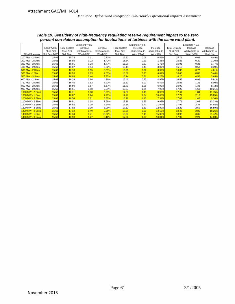
Manitoba Hydro Wind Integration Sub-Hourly Operational Impacts Assessment
Table 19. Sensitivity of high-frequency regulating reserve requirement impact to the zero percent correlation assumption for fluctuations of turbines with the same wind plant.
Exponent = 0.5 Exponent = 0.6 Exponent = 0.7Load Y2009 Total System Increase Increase Total System Increase Increase Total System Increase Increase
Fluct Dist Fluct Dist attributable to attributable to Fluct Dist attributable to attributable to Fluct Dist attributable to attributable toWind Scenario Std Dev (MW) Std. Dev. Wind (MW) Wind (%) Std. Dev. Wind (MW) Wind (%) Std. Dev. Wind (MW) Wind (%)
100 MW - 2 Sites 15.63 15.74 0.11 0.71% 15.72 0.09 0.59% 15.71 0.08 0.49%200 MW - 2 Sites 15.63 15.85 0.22 1.42% 15.84 0.21 1.35% 15.83 0.20 1.30%250 MW - 2 Sites 15.63 15.91 0.28 1.77% 15.90 0.27 1.76% 15.91 0.28 1.77%400 MW - 2 Sites 15.63 16.07 0.44 2.82% 16.11 0.48 3.07% 16.16 0.53 3.39%500 MW - 2 Sites 15.63 16.18 0.55 3.51% 16.25 0.62 3.99% 16.35 0.72 4.61%500 MW - 1 Site 15.63 16.26 0.63 4.03% 16.36 0.73 4.69% 16.48 0.85 5.46%500 MW - 3 Sites 15.63 16.09 0.46 2.97% 16.14 0.51 3.26% 16.20 0.57 3.65%600 MW - 2 Sites 15.63 16.29 0.66 4.20% 16.40 0.77 4.95% 16.55 0.92 5.91%750 MW - 2 Sites 15.63 16.45 0.82 5.23% 16.63 1.00 6.42% 16.88 1.25 8.00%800 MW - 2 Sites 15.63 16.50 0.87 5.57% 16.71 1.08 6.92% 16.99 1.36 8.72%900 MW - 2 Sites 15.63 16.61 0.98 6.24% 16.87 1.24 7.93% 17.23 1.60 10.21%1000 MW - 2 Sites 15.63 16.71 1.08 6.91% 17.03 1.40 8.96% 17.47 1.84 11.75%1000 MW - 1 Site 15.63 16.87 1.24 7.91% 17.27 1.64 10.48% 17.79 2.16 13.85%1000 MW - 3 Sites 15.63 16.54 0.91 5.85% 16.78 1.15 7.34% 17.09 1.46 9.36%1100 MW - 2 Sites 15.63 16.81 1.18 7.58% 17.19 1.56 9.99% 17.71 2.08 13.33%1200 MW - 2 Sites 15.63 16.92 1.29 8.24% 17.36 1.73 11.04% 17.97 2.34 14.94%1300 MW - 2 Sites 15.63 17.02 1.39 8.90% 17.52 1.89 12.09% 18.22 2.59 16.59%1400 MW - 2 Sites 15.63 17.12 1.49 9.55% 17.69 2.06 13.15% 18.48 2.85 18.26%1400 MW - 1 Site 15.63 17.34 1.71 10.92% 18.03 2.40 15.35% 18.98 3.35 21.42%1400 MW - 3 Sites 15.63 16.90 1.27 8.10% 17.32 1.69 10.81% 17.92 2.29 14.63%
Page 61 3/1/2005
Attachment GAC/MH I-014
November 2013

Manitoba Hydro Wind Integration Sub-Hourly Operational Impacts Assessment
5.2 Intra-Hour Load Following (Total Regulation) Impact Analysis
5.2.1. Generic Concept Load following (LF) is the service provided to follow the slower variations in system load as demand cycles throughout its daily pattern. As previously noted in section 2.2, the general analytical approach upon which this study is based differentiates load following from the regulation component in that LF describes the slower-varying, more correlated component of system load. It is further noted in section 2.2 and section 5.1.1, however, that many utilities operating in regulated market environments consider the portion of load following that occurs between pre-schedule periods as a component of system regulation. MH for example refers to the combination of their high-resolution response reserve and load following reserve as the “total regulating reserve.” MH’s total regulating reserve requirement comprises spinning reserve for tracking higher-frequency fluctuations in net load, spinning reserve for following within-hour load trends, and non-spinning reserve for following the slower ramping of net load throughout its daily cycle. The intra-hour load following impact analysis for this study actually assesses the impact of wind generation on this “total regulating reserve quantity.
It should be noted that load following impacts can comprise several components including increased production costs due to less optimal dispatch of units associated with ramping constraints, increased cycling of units to follow load, and increased opportunity costs associated with maintaining reserves to follow load between pre-schedule periods. This study analyzes only the latter of these impacts. Although the opportunity cost associated with this additional reserve must be determined from the custom scheduling tools, developed by Synexus Global, and used by Manitoba Hydro, the impact on the amount of reserves to be carried can certainly be quantified. The load following impact assessment methodology utilized for this study quantifies the extent to which the fluctuations of wind generation increase the amount of reserves MH holds to accommodate the total system intra-hour fluctuation. As noted in section 2.2, it is assumed that the inter-hour load following impacts are quantified as part of the subsequent short-term hydraulic planning simulation study.
MH is currently ahead of most North American utilities in the sense that MH currently calculates the amount of total regulating reserve carried for different load periods -- hour of the day and month of the year -- rather than simply carrying a fixed reserve amount for all hours irrespective of expected total load magnitude or variability. The total regulating reserve requirement specification method that MH currently utilizes15 is called the Hourly Total Regulation Requirement Methodology (HTRRM). The reserve values determined from the HTRRM are based on the statistical characteristics of the distribution of the variation of the 4-sec system load from the hourly average system load value as developed from historical load data. The result of this analytical approach is a specified reserve requirement for each hour of the day for each month of the year. The current
15 Tyler Black, Manitoba Hydro Internal Document, “Manitoba Hydro’s Regulation Reserves”.
Page 62 3/1/2005
Attachment GAC/MH I-014
November 2013

Manitoba Hydro Wind Integration Sub-Hourly Operational Impacts Assessment
HTRRM method, which is used by MH's system operators to determine the regulating reserve held for each hour, is based on reserving sufficient capacity to cover the fluctuations expected for a percent of time (HTRRM-CP85). In reviewing the adequacy of the current HTRRM – CP85 method under increasing wind penetration levels, it was recognized that the probability of large changes in net load increase rapidly as wind penetration levels increase as a percentage of system peak load. This fact is discussed in more detail in the analysis of 10-minute net load fluctuations in section 5.3. The HTRRM – CP85 does not capture the impact of the larger reserve deficits associated with these more extreme net load changes. Consequently, an extension of the current HTRRM method was utilized to assess the additional reserve required to maintain a specified MW magnitude differential between the reserve value and the largest anticipated fluctuation magnitude (HTRRM-Equivalent Residual) as compared to the current criteria of expected percent of the time for which the magnitude of fluctuations exceeds reserves. The HTRRM-Equivalent Residual approach provides an assessment of the impacts on the additional total regulating reserves required to maintain the magnitude of inadvertent tie-line interchanges at levels currently resulting from load only. Manitoba Hydro noted that it may have to alter its current operating procedures so as to ensure that that the magnitude of inadvertent interchanges with its tie-line neighbors do not significantly increase and to ensure that current NERC performance levels are maintained . Because it is not clear whether Manitoba will continue to schedule reserves according to the CP85 method or move to the Equivalent Residual methdod, the impact of wind generation on total regulating reserve is calculated using both methods to provide a range of possible total regulating reserve impacts.
5.2.2. Specific Manitoba Hydro Assessment Method Load and Wind Generation Time Series Synthesis Descriptions Before describing the reserve requirement calculation utilized for the load following impact assessment, we need to explain how the future study year load and wind generation time series data utilized for the analysis is obtained. One-minute resolution wind generation and system load time series for the future Y2009/2010 load year are required for the load following impact assessment. Section 4.1 describes the process of obtaining 10-minute average wind generation data and hourly average system load data for the study year. Section 4.3 describes how 1-minute average wind generation data (use of Midwest U.S. data as proxy) and 1-minute average system load data (integration of actual measured EMS data) is obtained for Y2003/2004. Section 5.1.2 describes how this Y2003/2004 base year data is used to obtain the high-frequency fluctuation component of the load and wind generation time series, which is then appropriately scaled to represent the Y2009/2010 high-frequency fluctuation time series for load and the various wind capacity scenarios. The load following assessment algorithm, however, requires the complete study year time series, not just the high-frequency fluctuation component. Obtaining the full load time series for a future year based on a historical time series or the full wind generation series for a specified wind capacity from a generation time series of a different capacity level is more complicated because the statistical correlation between the various time resolution components that constitute the series differ.
Page 63 3/1/2005
Attachment GAC/MH I-014
November 2013

Manitoba Hydro Wind Integration Sub-Hourly Operational Impacts Assessment
For example, as discussed in Section 5.1.2, the high-frequency fluctuation component of the wind generation time series for one installed capacity level is scaled to represent the time series of another capacity level using a multiplier of the square root of the ratio of the two capacity levels. This multiplier applies because it is assumed that the high-frequency fluctuation from the output of additional wind turbines is statistically uncorrelated. The slower fluctuations of output on the order of 5-15 minutes that will affect the intra-hour load following reserve component cannot be reasonably assumed to be uncorrelated, however. Thus, the same multiplier that is used to convert the high-frequency component cannot be used for the load following component16. As a result, a more detailed process is utilized to obtain the complete 1-minute time series for the future study year. The approach utilized is based on the decomposition of the 1-minute resolution time series into 3 components, each being a 1-minute resolution time series:
1. High frequency minute-by-minute fluctuation2. Intra-hour slow varying fluctuation with respect to the smooth inter-hour ramping3. Smooth inter-hour ramping
Using the measured Y2003/2004 1-minute resolution system load data provided, the first two load components identified above are extracted for the historical data period. The two corresponding components for the Y2009/2010 time series are synthesized from these historical period components by applying appropriate scaling factors. The Y2009/2010 hourly resolution load forecast provided by Manitoba Hydro is converted to a smooth, 1-minute resolution inter-hour ramping component through a process that conserves the hourly energy. The complete Y2009/2010 1-minute resolution system load time series is obtained by summing these three individual components. The detailed process utilized is presented in Appendix 2 section A2.1.
The approach for synthesizing the various Y2009/2010 capacity level wind generation time series is similar to the process used to synthesize the system load time series. Again, we consider the decomposition of wind generation into 3 components. Each component is constructed for the projected wind capacity for the study. Then the wind generation time series is obtained by the superimposing of the three individual components. The difference in this process and the process utilized for the load involves input data series utilized to obtain the individual component series. The detailed process utilized is presented in Appendix 2section A2.2.
Load Following Impact Assessment Calculation -- HTRRM – CP85 Impact Approach
As noted in Section 5.2.1, MH currently utilizes the HTRRM approach to determining the total regulating reserve (where the term “total regulating reserve” encompasses both the minute-to-minute fluctuations and slower varying sub-hourly load following) to be maintained for each hour of each month. The first portion of the LF impact assessment determines the additional total regulating reserve requirement that is calculated for
16 Eric Hirst and Jeffrey Hild, “Integrating Large Amounts of Wind Energy with a Small Electric Power System,” April, 2004.
Page 64 3/1/2005
Attachment GAC/MH I-014
November 2013

Manitoba Hydro Wind Integration Sub-Hourly Operational Impacts Assessment
various wind scenarios utilizing the current HTRRM calculation method (CP85). The approach utilized is as follows:
1. Determine load-only total regulating reserve requirement. Each 1-minute pointof the Y2009/2010 1-minute load time series is subtracted by the correspondinghourly average load value to obtain a time series of Y2009/2010 load 1-mindeviations. For each calendar month, a separate distribution for each clock hourof the day is formed. Each of these clock hour distributions comprises thecollection of maximum positive 1-minute deviations occurring within that clockhour for each of the days within the respective calendar month. The regulatingreserve to be maintained for a given clock hour for a given month is designated asthe 85th percent cumulative probability of the corresponding distribution ofmaximum positive 1-minute deviations (thus the “CP85” designation). Thisprocess is performed for each month of the Y2009/2010 study year to obtain theregulating reserve to be maintained for accommodating the fluctuations of theload alone.
2. Determine net load total regulating reserve requirement for wind scenarios. Fora given wind capacity scenario, each 1-minute point of the associated 1-minutewind generation time series is subtracted from the corresponding Y2009/2010 1-minute load time series to obtain a Y2009/2010 net system load time series for thespecific wind capacity scenario. Each 1-minute point of this 1-minute net loadtime series is then subtracted by the corresponding hourly average net load valueto obtain a time series of Y2009/2010 net system load 1-min deviations for thewind capacity scenario. The same process identified in #1 for the system load isthen followed for the net load time series to obtain the regulating reserve to bemaintained for accommodating the aggregate fluctuations of the load and thewind generation output for the associated wind capacity scenario.
3. Determine total regulating reserve impact for wind scenarios. For each windgeneration capacity scenario, the difference in the regulating reserve requirementis determined by subtracting the reserve values calculated for the load alone fromthe reserve values calculated for the aggregate load and wind fluctuation. Thiscalculation is made for all 288 hourly regulating reserve values that represent thehourly values (24) for each of the 12 months.
It should be noted that this process differs from MH’s actual regulating reserve requirement procedure in two respects.
1. MH procedure actually looks at the deviation of 4-second EMS load data pointfrom the hourly average rather than the deviation of the 1-minute data point usedfor this analysis. MH allocates regulating reserve to follow the fast minute-to-minute fluctuations of system load and the slower intra-hour fluctuations aroundthe trend of load from hour to hour to maintain NERC system performanceindices within appropriate ranges. By definition, NERC CPS1 and CPS2 measurethe utility’s ability to follow load fluctuations down to only a resolution of 1minute. Assuming that MH does not try to control generation to match these sub-minute fluctuations, the sub-minute fluctuations of load manifest themselves as
Page 65 3/1/2005
Attachment GAC/MH I-014
November 2013
Manitoba Hydro Wind Integration Sub-Hourly Operational Impacts Assessment
fluctuations on MH’s tie flow. The extent of these fluctuations should not impact regulating reserve, but rather might have some impact on MH’s allocation of TRM. Thus, utilizing the deviation of the 1-minute average rather than the 4-second average provides a better metric of the impact of wind generation on the ability to maintain NERC control performance standards. It should be noted, however, that the matrix of Total Regulation Reserve used by Manitoba Hydro, which has proven to result in acceptable NERC CPS performance, is based on the deviation of 4-second values from the hourly average. Furthermore, historical data indicates that the distribution of this reserve matrix is approximately 20 MW higher than the CP85 matrix calculated using the deviation of 1-minute average values from the hourly average value.
2. MH actually adds an additional 30 MW buffer to the calculated regulating reservevalue for each hour of each month to accommodate the uncertainty in loadforecasts. Since it was decided that the forecast uncertainty assessment task of theoriginal proposal was shifted to the subsequent hydraulic simulation study andsince our analysis is focused on the incremental requirement for wind generation,we did not include the additional 30 MW in the calculations.
Load Following Impact Assessment Calculation -- HTRRM – Equivalent Residual Impact Approach
As noted above, the HTRRM – CP85 does not capture the impact of the larger reserve deficits associated with the more extreme net load changes that occasionally occur with high levels of wind generation relative to system load levels. Consequently, the LF impact assessment also includes a determination of the additional total regulating reserve requirement calculated utilizing the extended HTRRM calculation method (Equivalent Residual). The HTRRM – Equivalent Residual approach is utilized in the LF impact analysis as follows:
1. Determine load-only MW residual. The exact process described in Step #1 of theHTRRM-CP85 approach is performed to obtain the 85th percent cumulativeprobability of the distribution of maximum positive 1-minute deviations for eachhour of the day for each month of the year. This process is performed for eachmonth of the Y2009/2010 study year. The result is 12 x 24 matrix of CP85 valuesof MW deviations of 1-minute average load from the corresponding hourlyaverage load value. A similar 12 X 24 matrix of the largest (CP100) deviation of1-minute positive deviation from hourly average is then determined for the sameY2009/2010 data set. The “uncovered” MW differential between the CP100 andthe CP85 values is calculated for each of hour of each month, resulting in 12 x 24matrix of MW residual values. Rather than use each of these 288 values, the newapproach identifies a single target residual value. This value is taken as the 90th
percent cumulative probability value of the matrix of 288 values. The CP90 valueis selected to ensure that the impacts of the load data errors discussed in section4.3.1 do not unduly affect the results.
2. Determine net load CP value that yields equivalent residual. The general processdescribed in Step #2 of the HTRRM-CP85 approach is performed to obtain a
Page 66 3/1/2005
Attachment GAC/MH I-014
November 2013

Manitoba Hydro Wind Integration Sub-Hourly Operational Impacts Assessment
specified cumulative probability of the distribution of maximum positive 1-minute deviations for each hour of the day for each month of the year. The specified cumulative probability percentage utilized (“equivalent residual CP”) for each wind scenario is selected to yield the same target residual value as obtained for the load only scenario when the CP90 value of the 288 matrix values is calculated.
3. Determine additional total regulating reserve to accommodate wind generation.For each wind capacity scenario, the 12 x 24 matrix of equivalent residual CPvalue of the distributions of maximum positive 1-minute deviations for each hourof the day for each month of the year is taken from Step #2 above. Each value inthe load-only CP85 matrix of maximum positive 1-minute deviations is thensubtracted from the corresponding value in the net load equivalent residual CPmatrix. The resulting matrix of values is the additional total regulating reserverequirement for each hour of each month that must be held to accommodate windgeneration.
5.2.3. Results and Analysis HTRRM – CP85 Impact Approach The procedure described in the previous subsection was first performed for the Y2003/2004 load data to obtain the total regulating reserve requirement values for comparison with the existing values utilized by Manitoba Hydro. Table 20 presents the raw total regulating reserve requirement calculated for each hour of each month based on the MH Y2003/2004 load data. The relative magnitudes of the calculated regulating reserve values shown in Table 20 correlate to the general ramping trends that exist within the Y2003/2004 load data. Figure 27 shows the average hourly load calculated for all hours occurring during the Y2003/2004 load time series. Note that the most significant ramping of load occurs during the following periods:
Morning ramp-up – on average, the steepest load ramp occurs during the morningramp from 5 a.m. to 8 a.m., during which time the average ramp approaches 180MW/hrNightly ramp-down – on average, the second steepest load ramp occurs betweenhours 9 p.m. to 1 a.m., during which time the average ramp approaches 160MW/hrEvening ramp-up – on average, the third steepest load ramp occurs during theearly evening ramp from 5 p.m. to 7 p.m., during which time the average rampapproaches 60 MW/hr
The steepest ramping periods that can be seen in Figure 27 correspond to the largest total regulating reserve values shown in Table 20. This is expected, as the largest deviations of intra-hour data points from the hourly average should occur during the steepest ramping periods.
Page 67 3/1/2005
Attachment GAC/MH I-014
November 2013

Manitoba Hydro Wind Integration Sub-Hourly Operational Impacts Assessment
Table 20. Raw total regulating reserve requirement values calculated for MH Y2003/2004 load data.
Hr Jan Feb Mar Apr May Jun Jul Aug Sep Oct Nov Dec Sum1 65.5 56.6 55.6 45.8 50.2 50.9 51.7 58.3 48.2 45.1 63.6 70.7 662.02 36.6 41.8 34.8 37.6 38.6 38.8 38.5 46.5 34.7 33.1 43.2 45.1 469.23 31.0 34.7 30.8 33.3 26.7 31.0 28.6 38.8 32.6 33.7 37.9 31.7 390.64 32.3 32.5 32.4 44.0 36.3 30.1 22.0 28.6 39.6 38.9 39.0 38.1 413.75 42.7 44.4 47.7 85.7 74.9 48.8 33.4 55.1 67.4 83.0 48.6 40.9 672.66 83.1 78.0 104.4 141.2 149.6 143.1 92.9 90.3 147.5 143.9 91.7 76.6 1342.27 132.0 141.2 126.9 110.3 122.1 132.8 131.6 122.8 104.5 113.3 149.4 146.7 1533.58 109.0 76.0 85.5 68.5 66.0 81.7 93.8 95.8 71.1 65.3 91.9 109.8 1014.29 56.2 41.6 49.6 53.3 50.9 57.5 86.0 80.4 50.9 48.5 56.3 53.2 684.2
10 53.0 47.6 52.4 35.5 50.6 55.6 59.3 74.3 45.5 39.9 57.9 49.0 620.411 38.5 54.9 45.0 36.9 34.8 49.9 43.8 73.0 39.7 39.6 42.6 53.8 552.312 42.4 44.3 43.2 46.8 42.7 37.2 41.4 42.8 43.1 51.0 38.9 44.2 517.713 64.1 62.3 66.7 60.2 35.8 37.8 31.9 35.0 42.7 44.3 54.4 60.0 595.114 42.9 41.5 40.3 59.5 38.7 46.4 32.0 34.9 38.4 43.1 34.1 43.6 495.515 37.6 34.6 32.4 38.7 34.9 44.4 39.0 35.7 38.9 34.5 41.5 43.1 455.316 59.3 58.9 37.7 39.5 36.6 42.3 36.0 40.7 54.8 50.2 67.1 85.0 607.917 129.8 85.6 63.9 38.1 38.1 35.7 31.9 31.8 34.6 69.9 142.5 151.7 853.418 70.6 83.7 54.8 45.2 71.8 81.4 64.4 67.3 61.4 70.5 52.5 42.1 765.619 44.9 41.0 87.5 39.8 58.8 51.2 65.1 65.7 62.6 54.6 60.3 51.2 682.620 45.4 43.9 36.4 71.0 42.5 46.6 46.4 50.4 41.1 47.6 44.1 43.1 558.521 46.5 47.7 42.7 42.4 46.0 43.2 38.4 49.1 72.0 66.8 51.2 40.8 586.622 61.8 69.5 70.1 94.5 114.6 67.0 65.5 86.8 96.4 82.4 71.7 66.3 946.323 82.9 83.4 87.2 109.7 117.3 124.3 141.9 128.6 110.8 97.1 82.6 91.8 1257.424 101.9 90.9 93.7 82.0 79.6 96.1 95.4 100.3 72.9 86.1 108.3 108.3 1115.2
Sum 1509.8 1436.6 1421.7 1459.1 1458.0 1473.1 1410.8 1532.7 1450.8 1482.3 1570.5 1586.7 17791.9
MH Y2003/2004 Hourly Average Load
2000
2100
2200
2300
2400
2500
2600
2700
2800
1 2 3 4 5 6 7 8 9 10 11 12 13 14 15 16 17 18 19 20 21 22 23 24
Hour of Day
Figure 27. Manitoba Hydro Y2003/2004 hourly average load per hour of the day.
Page 68 3/1/2005
Attachment GAC/MH I-014
November 2013
Manitoba Hydro Wind Integration Sub-Hourly Operational Impacts Assessment
In addition to reviewing the calculated Y2003/2004 total regulating reserve values relative to the shape of the average load curve, we also want to compare the calculated values with those calculated by Manitoba Hydro for other years of data. MH personnel supplied two spreadsheets related to the HTRRM-CP85 total regulating reserve calculations made for the Manitoba Hydro Y1999/2000 load year:
spreadsheet titled "4 second monthly percents final.xls" -- contains total regulating reserve values calculated based on deviation of 4-second load data points from hourly average with the additional 30 MW buffer added spreadsheet titled "monthly regulation percentage.xls" – contains the raw total
regulating reserve values calculated based on deviation of 1-minute average load data points from hourly average.
The values in the second spreadsheet represent the same quantities calculated from the HTRRM – CP85 load following impact assessment for this study. Table 21 shows the difference in the raw total regulating reserve values that we calculated for the Y2003/2004 load data and the values contained in the "monthly regulation percentage.xls" spreadsheet, which were calculated by MH personnel for the Y1999/2000 load data. The red values in parentheses represent instances where the Y2003/2004 raw total regulating reserve values are less than the value supplied in the spreadsheet. Note that significant differences exist with the total regulating reserve values calculated for Y2003/2004 being smaller for the majority of hours. Although it is difficult to discern any definable trends other than the generally smaller values for Y2003/2004, Table 21 does appear to show the following sub trends:
Large negative deviations from the supplied Y1999/2000 values (presenting a lower regulating reserve requirement) tend to consistently occur during the late night/early morning hours of 11 p.m. – 2 a.m. and during the morning hours of 6 a.m. – 8 a.m. These are generally the periods of steepest ramping for the Y2003/2004 load data. Large positive deviations from the supplied Y1999/2000 values (presenting a
higher regulating reserve requirement) tend to consistently occur during the during the morning hours of 4 a.m. – 6 a.m. and during evening hours of 6 p.m. – 9 p.m. and. These are periods of milder ramping for the Y2003/2004 load data. Deviations are relatively small during the low ramping period of the day.
Without examining the actual data from which the Y1999/2000 total regulating reserve values were calculated, it is impossible to assess the exact reason for some of the significant differences in the calculated values. It is within reason that the nature of the fluctuation existing in the underlying data might differ significantly as the number of samples constituting each monthly/hourly distribution is relatively small for one calendar year of data, ranging from 28-31 samples. Regardless, the calculations for the Y2003/2004 data do seem reasonable relative to the underlying ramping in the data, and the calculations associated with the specified method were verified to ensure accuracy of results.
Page 69 3/1/2005
Attachment GAC/MH I-014
November 2013

Manitoba Hydro Wind Integration Sub-Hourly Operational Impacts Assessment
Table 21. Difference in raw total regulating reserve requirement values calculated for Y2003/2004 load data and values contained in MH supplied spreadsheet calculated for
Y1999/2000. Hr Jan Feb Mar Apr May Jun Jul Aug Sep Oct Nov Dec Sum
1 (16.1) (16.8) (20.5) (38.3) (29.1) (35.3) (59.2) (32.6) (21.8) (32.9) (22.6) (20.9) (345.9)(7.7) (3.3) (8.7) (7.8) (18.1) (23.2) (41.2) (9.8) (7.9) (15.3) (4.7) (5.8) (153.4)(4.4) (0.9) (13.6) (8.9) (36.0) (0.4) (2.3) (1.6) (60.8)(2.5) (3.4) (1.8) (4.5) (20.9) (6.2) (5.9)(5.2) (10.5) (12.0) (2.4) (10.0)
(14.0) (15.5) (9.7) (17.0)(29.5) (16.0) (6.5) (28.9) (25.6) (7.7) (58.0) (71.0) (11.6) (206.9)
(19.6) (8.2) (35.6) (66.2) (50.6) (39.9) (31.7) (50.4) (55.1) (10.2) (5.9) (369.0)(7.5) (2.4) (20.5) (24.8) (21.2) (19.9) (20.6) (3.7) (7.0) (114.9)(6.5) (1.6) (11.8) (17.1) (3.7) (10.9)
(5.9) (4.8) (12.8) (5.1) (17.5) (0.8) (19.3)(1.2) (6.3) (54.5) (14.9) (7.7) (32.8)
(9.9) (15.4) (18.6) (2.6) (9.0) (10.1) (0.7) (10.1) (46.6)(10.5) (29.9) (4.7) (6.0) (10.2) (1.3) (13.0) (11.7) (64.6)(6.5) (17.7) (16.8) (3.1) (76.3) (6.3) (11.1) (125.2)(0.2) (12.5) (51.0) (0.5) (9.9) (3.4) (40.3)(2.6) (5.1) (4.2) (4.1) (8.5) (17.7) (6.0) (6.9) (11.6)
(4.8) (2.1)(2.7) (7.6) (19.6) (0.4) (23.9)
(3.8) (1.2) (3.8) (9.3) (1.6) (13.6) (6.8) (1.6) (0.8) (5.1)(2.3) (33.1) (12.1) (12.6) (6.4) (3.3) (8.4) (12.9)
(1.8) (1.6) (4.1) (9.9) (1.5)(3.4) (24.1) (12.7) (35.0) (22.1) (26.9) (21.9) (67.6)
(28.1) (26.1) (20.4) (32.8) (46.4) (25.5) (52.6) (27.4) (55.5) (28.7) (12.7) (34.0) (390.3)
(118.1) (196.6) (81.3) (140.5) (136.3) (195.9) (61.7) (45.6) (76.7) (89.8) (114.1) (1238.5)
23 1.3 4.9 0.1 1.04 10.3 0.3 4.9 8.9 6.3 2.65 32.9 35.6 13.3 6.4 19.9 25.2 45.7 138.96 0.9 35.9 74.7 82.0 49.2 18.7 50.1 49.6 304.97 20.5 21.8 5.48 4.69 7.3 1.5 3.8
10 1.6 5.8 1.5 1.7 0.1 16.3 2.811 8.1 0.8 6.1 2.1 1.2 9.312 4.5 13.3 4.8 7.3 16.6 1.9 3.513 5.6 6.3 11.9 5.914 12.7 1.1 8.3 0.715 0.7 0.7 1.9 6.5 2.816 2.3 1.3 18.5 7.4 1.5 6.217 12.9 2.4 19.9 8.218 1.6 13.8 1.3 33.8 40.0 26.8 31.6 26.6 34.1 2.0 204.719 1.0 9.7 6.7 8.1 19.5 11.2 2.2 4.320 29.8 5.2 2.321 0.5 7.1 4.2 31.0 22.622 1.3 50.2 68.7 19.7 17.9 34.5 19.6 192.823 2.1 1.7 9.2 34.4 31.224
Sum 18.1
The HTRRM – CP85 total regulating reserve requirement calculations were next completed for the net system load series determined from the synthesized 1-minute resolution MH Y2009/2010 system load and wind generation output series for each of the identified wind generation capacity scenarios. This process yielded 23 total regulating reserve requirement tables (1 for MH system load and 22 for the net load profiles resulting from the identified wind scenarios). Table 22 shows the total regulating reserve values calculated for the Y2009/2010 load alone. The relative magnitudes of the values for specific hours are very similar to the values calculated for the Y2003/2004 load, but in general, the total regulating reserve for any given hour is slightly higher for Y2009/2010 relative to Y2003/2004. This can be quickly assessed by looking at the “Sum” value for any month or hour. This value is used only as a summary metric for comparing the relative amounts of total regulating reserve represented by the matrix of hourly values determined for the multiple cases considered.
Page 70 3/1/2005
Attachment GAC/MH I-014
November 2013

Manitoba Hydro Wind Integration Sub-Hourly Operational Impacts Assessment
Table 22. Raw total regulating reserve requirement values calculated for synthesized MH Y2009/2010 1-minute load time series.
Hr Jan Feb Mar Apr May Jun Jul Aug Sep Oct Nov Dec Sum1 64.8 53.9 55.4 49.2 64.5 54.3 65.8 69.9 54.2 44.9 70.5 74.1 721.42 37.5 41.8 39.9 45.1 44.0 49.9 58.1 54.8 37.2 40.7 39.3 46.3 534.83 33.7 36.5 35.9 36.4 38.7 43.0 42.5 47.8 32.1 39.5 40.0 32.9 459.14 46.7 36.8 36.9 47.6 51.2 42.6 41.4 37.4 39.1 50.2 40.2 35.4 505.55 52.2 52.2 53.6 115.2 94.8 72.0 46.0 68.2 92.2 111.1 49.2 53.2 859.86 119.8 96.0 105.2 132.5 137.7 141.7 133.0 117.2 150.4 153.2 92.0 102.7 1481.57 153.6 159.3 114.3 101.3 98.8 144.8 136.7 131.6 124.1 119.8 159.8 151.8 1595.98 113.4 89.0 87.7 62.5 94.4 82.7 112.4 94.6 69.8 69.6 105.5 125.7 1107.39 53.0 40.1 51.4 48.8 60.4 53.2 72.4 77.3 54.9 44.0 47.6 55.3 658.3
10 61.3 56.4 59.3 56.7 52.5 57.8 56.6 62.5 44.7 46.6 70.1 49.9 674.511 52.3 60.0 62.9 48.6 43.4 47.8 52.1 71.8 41.4 47.1 44.6 48.3 620.112 52.3 46.0 45.3 52.4 49.2 42.2 32.1 48.6 44.3 56.7 37.5 49.6 556.413 65.5 67.8 70.5 48.0 47.2 44.2 33.7 36.6 40.4 51.3 57.7 63.0 625.814 50.4 53.4 41.6 54.9 48.3 47.7 36.7 41.7 43.1 55.2 34.8 43.4 551.215 46.6 41.8 36.4 47.2 38.0 47.3 36.4 45.5 48.3 44.6 41.3 44.2 517.416 73.5 56.5 39.5 42.8 44.3 43.5 45.2 44.9 56.5 55.1 82.7 85.5 670.017 123.1 81.9 58.1 40.4 42.1 41.6 37.2 35.7 41.4 49.7 123.1 169.1 843.318 74.1 95.3 43.7 59.6 67.4 62.7 48.4 59.8 56.8 55.0 73.4 66.1 762.419 47.8 45.4 78.4 50.5 58.9 53.5 48.8 65.6 72.9 55.6 58.0 51.4 686.820 48.7 47.2 48.2 77.8 61.7 54.9 52.6 67.1 50.8 50.4 51.2 41.7 652.521 51.1 54.2 48.5 47.5 60.3 52.6 47.0 70.9 87.0 70.6 50.3 46.9 686.822 63.5 69.0 56.6 93.7 100.7 91.7 80.5 137.2 118.9 112.9 78.3 67.0 1070.123 101.3 94.7 88.0 111.9 130.7 115.6 164.3 138.5 121.3 115.6 105.8 123.8 1411.524 122.0 102.7 92.4 66.8 79.1 99.5 114.3 103.8 71.1 72.8 112.3 127.7 1164.4
Sum 1708.5 1577.9 1449.6 1537.3 1608.5 1586.7 1594.1 1729.3 1593.2 1612.0 1665.1 1754.8 19416.8 Table 23 shows the MW differentials of the total regulating reserve calculated for the Y2009/2010 load alone and the reserve values calculated for the net system load resulting from the integration of 250 MW of total wind capacity at a single site. Note that the values shown in Table 23 are the DIFFERENTIAL values between the cases. As noted previously, the red values in parentheses indicate a negative change or reduction in total regulating reserve requirement from the base case of the load alone. Table 23 shows that there are both hours for which the wind generation fluctuations increase and decrease the total regulating reserve requirement. In general, however, the reserve values increase as indicated by the positive 1466 MW sum value shown in the summary table. Unlike the trends in the load alone case, it is difficult to discern a reasonable correlation between the relative magnitudes of the reserve differentials and the relative ramping of the load and wind plant output. Figure 28 shows the hourly average load and wind plant values for the 24 hours of the study year. Note that the scales are selected to emphasize the average trending. Comparison of Table 23 and Figure 28 reveals that larger reserve increases occur during periods where either the total regulating reserve for the load alone is relatively small due to the load being relatively flat during the period or during periods where the load and wind ramp in opposite directions. Examples include:
Hours 24-4 – relatively large reserve increases as high as 25 MW as the reserve maintained for load alone is relatively small. Although wind generation is relatively flat during this period also, the standard deviation of fluctuation of wind is much larger than for load of similar magnitude.
Page 71 3/1/2005
Attachment GAC/MH I-014
November 2013

Manitoba Hydro Wind Integration Sub-Hourly Operational Impacts Assessment
Hours 12-17 – relatively large reserve increases as high as 40 MW as the load is either relatively flat or the wind and load are ramping in opposite directions.
The patterns aren’t completely obvious for all periods as the reserve values calculated are statistical metrics that may not always exactly correlate with the average values that are plotted for visual reference.
Table 23. Difference in raw total regulating reserve requirement values calculated for Y2009/2010 load data alone and values calculated for net load resulting from 250 MW of
wind generation capacity at a single site.
Hr Jan Feb Mar Apr May Jun Jul Aug Sep Oct Nov Dec Sum1 0.58 16.38 16.72 4.82 16.51 4.17 13.57 3.62 8.07 13.43 3.54 2.90 104.312 10.47 4.93 8.73 8.63 15.03 6.81 8.74 5.56 9.48 7.55 10.57 4.16 100.673 11.48 8.74 11.91 19.66 9.48 8.63 10.55 14.58 16.74 9.47 16.57 24.55 162.344 (1.00)
(5.85) (1.46) (11.78)(0.60)
(2.56) (0.90)(3.66) (0.53)
(0.05) (3.85) (4.33)(2.27) (1.52) (0.44)
(3.01)
(2.49)
(1.65) (2.44)(2.16) (6.82) (1.42)
(1.54)
(0.21)
(1.96) (11.33)
9.85 25.28 12.76 9.66 5.28 10.95 3.90 20.72 11.58 4.01 12.30 125.295 5.28 5.70 7.76 4.03 12.12 10.20 2.44 9.64 2.33 40.416 7.38 2.12 13.20 7.31 14.29 0.63 4.82 4.88 7.41 6.92 4.83 73.207 1.87 9.72 8.96 14.66 5.55 21.56 11.21 8.90 4.11 6.31 89.398 4.39 6.67 16.28 4.76 3.81 8.37 21.74 4.90 3.79 1.16 71.689 8.55 17.88 18.24 13.26 4.08 5.44 15.92 10.90 7.06 93.10
10 11.76 0.64 3.04 9.47 2.00 5.29 7.06 10.84 6.65 52.5211 1.97 23.74 4.77 7.91 3.07 9.40 5.78 11.56 3.28 9.97 5.03 83.4812 8.49 14.99 4.63 4.94 15.14 10.95 22.00 9.68 6.84 1.90 9.44 4.16 113.1413 6.03 15.56 11.55 10.36 10.78 3.13 11.88 17.13 13.46 8.44 12.02 117.8414 7.37 8.41 2.95 12.32 13.68 13.28 6.86 9.21 9.66 12.43 11.20 11.78 119.1415 1.16 11.36 10.58 6.45 16.82 5.20 12.62 10.89 5.14 7.76 10.23 6.43 104.6416 5.40 11.28 12.90 34.12 16.25 20.28 6.69 10.36 15.91 10.36 0.01 9.47 153.0317 6.93 2.47 15.15 8.84 12.27 39.23 14.54 19.58 5.62 0.14 120.6818 0.92 14.00 2.50 10.84 10.87 5.67 6.09 10.91 1.22 52.6219 9.85 4.40 9.74 12.64 8.69 8.55 9.10 3.16 9.62 5.92 8.77 88.9020 7.31 1.69 6.28 7.40 20.94 6.68 7.38 6.37 10.76 4.57 4.34 14.74 98.4721 6.62 14.95 5.78 6.14 6.53 11.62 10.86 13.39 5.63 18.00 19.56 118.8922 8.39 4.85 16.82 5.21 6.91 5.11 13.93 1.58 17.35 9.47 4.98 3.70 98.3023 1.73 6.21 15.64 9.64 2.02 9.29 9.35 7.98 5.43 9.50 63.4924 8.90 6.43 10.61 9.38 13.76 15.05 8.04 3.44 7.34 2.26 10.56 5.76 101.52
Sum 85.32 91.29 176.82 151.44 142.44 96.02 157.97 128.42 138.93 111.84 108.09 78.01 1,466.59
Page 72 3/1/2005
Attachment GAC/MH I-014
November 2013

Manitoba Hydro Wind Integration Sub-Hourly Operational Impacts Assessment
Relative Ramping of Load and 250 MW Wind
2000
2100
2200
2300
2400
2500
2600
2700
2800
2900
3000
1 2 3 4 5 6 7 8 9 10 11 12 13 14 15 16 17 18 19 20 21 22 23 24
Hour of Day
Avg
. L
oad
(M
W)
75.00
80.00
85.00
90.00
95.00
100.00
Avg
. W
ind
Gen
(M
W)
AvgLoad
AvgWind
Figure 28. Relative ramping of average Y2009/2010 load and 100 MW wind plant generation production.
As stated previously, the standard deviation of fluctuation of wind generation output is much higher than system load on a per unit basis. Thus, as the capacity of the total wind plant being integrated approaches the same order of magnitude as the system load, the fluctuations in wind generation begin to dominate the net load fluctuations, significantly increasing the total regulating reserve values. Table 24 shows the differential in regulating reserve for the net load resulting from integrating a 500 MW wind plant at a single site. Note that there are many fewer hours for which the total regulating reserve decreases and higher magnitude increases in total regulating reserve when compared to the total regulating reserve impacts for the 250 MW wind plant case of Table 23. Similar progressions can be seen for the total regulating reserve requirement increases for the 750 MW and 1000 MW single site wind generation capacity scenarios shown in Table 25 and Table 26, respectively.
Page 73 3/1/2005
Attachment GAC/MH I-014
November 2013

Manitoba Hydro Wind Integration Sub-Hourly Operational Impacts Assessment
Table 24. Difference in raw total regulating reserve requirement values calculated for Y2009/2010 load data alone and values calculated for net load resulting from 500 MW of
wind generation capacity at a single site. MW Reg Reserve Requirement Differential for Load Alone and 500 MW Wind w/1Site
Hr Jan Feb Mar Apr May Jun Jul Aug Sep Oct Nov Dec Sum1 4.41 38.39 34.86 26.10 31.24 15.07 22.68 21.05 16.73 34.42 15.77 4.68 265.402 36.36 28.98 21.84 29.18 56.20 27.09 23.84 21.70 17.78 22.53 29.33 43.21 358.033 36.24 26.61 16.81 41.79 37.74 24.48 23.23 29.27 46.78 31.84 48.12 46.31 409.234 8.93 22.11 54.61 33.09 39.21 17.77 27.25 20.36 36.53 39.13 37.41 20.97 357.385 9.55 17.09 27.25 13.69 5.63 9.56 37.22 23.75 4.41 6.99 25.59 20.66 201.406 10.87 10.15 15.86 27.24 15.30 6.86 12.46 18.20 21.95 13.77 12.54 (0.86)
(8.91)(0.02)
(2.52) (0.24)(0.98)
(7.47)
164.347 7.01 30.86 16.01 37.07 26.93 48.76 37.28 19.93 8.99 13.76 11.78 249.478 2.90 24.85 27.28 7.44 9.25 10.77 26.03 49.45 23.21 24.09 25.12 230.389 17.76 32.01 49.86 38.00 18.44 2.60 5.04 15.48 41.13 37.85 30.16 14.14 302.48
10 16.56 11.67 14.15 24.45 23.97 9.74 21.74 18.36 30.09 28.55 7.39 26.35 233.0111 6.99 21.02 45.07 23.34 27.23 10.97 29.12 22.33 41.52 25.17 31.77 18.41 302.9412 18.37 41.57 18.37 21.27 31.91 24.45 55.58 30.39 17.31 14.60 28.45 21.74 324.0013 27.11 20.50 20.65 26.93 28.76 22.69 54.38 50.65 37.38 31.91 16.49 42.09 379.5414 15.37 27.48 16.94 41.73 36.39 40.33 29.54 34.14 40.36 46.13 33.20 23.84 385.4515 16.65 18.32 30.70 22.56 31.17 19.73 34.23 35.15 27.50 24.24 27.59 32.00 319.8416 6.25 21.96 38.89 65.69 33.42 39.50 28.48 30.75 46.65 29.10 1.51 4.47 346.6817 22.41 21.65 39.39 27.74 25.45 90.07 31.52 45.08 29.95 8.05 338.5618 16.43 45.24 28.87 22.21 2.75 30.35 27.32 44.12 28.15 7.65 17.75 269.8619 21.77 23.43 12.01 26.29 18.46 24.85 24.76 14.15 14.70 23.85 14.83 38.55 257.6620 21.57 25.52 18.32 23.86 44.11 27.03 24.26 17.52 25.37 22.16 25.82 51.03 326.5721 16.10 36.12 28.59 25.20 36.34 31.60 25.67 17.43 17.16 35.48 45.09 18.37 333.1522 13.88 13.10 36.76 13.75 20.25 15.89 26.23 17.65 26.28 21.06 26.05 20.53 251.4423 3.30 10.42 31.19 24.36 6.68 19.18 18.65 18.62 9.05 9.98 34.92 178.8824 12.53 15.05 21.26 25.18 29.44 22.87 11.73 25.72 21.44 22.96 17.30 12.45 237.94
Sum 344.40 474.00 676.63 685.25 666.33 476.64 716.05 604.82 698.69 612.04 554.59 514.17 7,023.62
Page 74 3/1/2005
Attachment GAC/MH I-014
November 2013
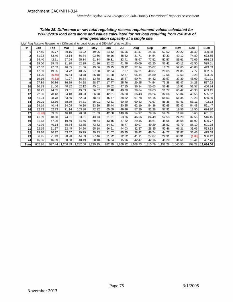
Manitoba Hydro Wind Integration Sub-Hourly Operational Impacts Assessment
Table 25. Difference in raw total regulating reserve requirement values calculated for Y2009/2010 load data alone and values calculated for net load resulting from 750 MW of
wind generation capacity at a single site. MW Reg Reserve Requirement Differential for Load Alone and 750 MW Wind w/1Site
Hr Jan Feb Mar Apr May Jun Jul Aug Sep Oct Nov Dec Sum1 17.45 65.77 59.15 54.22 49.95 24.42 36.06 41.47 24.16 57.52 29.22 31.49 490.882 61.73 63.49 43.14 56.74 93.56 49.16 58.32 31.71 44.54 47.33 49.12 74.80 673.653 64.40 42.51 27.94 65.34 61.84 49.31 33.41 48.67 77.52 52.57 85.61 77.09 686.234 19.00 39.45 91.20 52.98 61.10 32.02 41.48 40.09 62.25 56.42 60.12 43.50 599.615 27.07 47.03 46.05 31.06 19.56 29.15 60.12 37.14 35.07 18.79 52.65 45.88 449.596 17.59 19.35 34.72 48.25 27.58 12.84 7.67 34.21 40.87 29.65 21.85 7.77 302.357 14.25 (6.46)
(0.62)
(1.43)
(1.83)
46.54 33.78 56.18 51.28 82.77 65.44 34.80 17.58 17.63 9.28 423.068 19.16 41.27 56.54 13.78 18.11 15.87 50.74 84.42 39.57 37.39 45.09 421.319 27.89 60.86 86.79 64.58 28.67 17.77 25.76 29.25 74.54 73.38 53.47 34.25 577.22
10 16.83 31.06 40.32 52.12 45.51 20.62 47.85 36.34 50.63 56.48 16.91 51.57 466.2411 18.25 44.35 93.31 49.03 56.07 27.48 49.30 39.64 59.63 51.27 66.42 48.38 603.1512 22.96 70.43 34.18 40.93 56.78 42.81 86.60 66.43 36.24 32.66 55.04 40.56 585.6213 51.24 28.78 33.66 52.03 48.34 45.77 88.52 91.78 64.15 58.53 51.35 72.23 686.3614 30.01 52.86 38.69 64.61 55.01 72.81 60.40 60.83 71.67 85.35 57.41 53.11 702.7315 34.19 40.44 54.08 46.50 53.39 35.44 50.35 62.19 54.36 52.65 53.43 54.45 591.4716 22.73 52.73 71.14 103.80 72.22 65.59 46.46 57.29 91.28 57.91 19.56 13.50 674.2017 39.05 46.18 70.80 51.53 42.68 140.76 54.97 79.16 59.79 11.69 6.60 601.8118 41.09 18.50 74.61 53.81 43.73 21.01 53.26 46.66 84.49 52.53 24.20 32.56 546.4519 31.13 47.26 19.69 44.66 60.54 43.45 37.32 29.45 48.61 48.06 34.68 81.92 526.7720 41.79 40.14 30.64 63.65 73.82 54.81 46.77 30.07 49.29 38.92 43.79 88.10 601.7821 22.15 61.87 52.45 54.20 65.18 66.61 44.03 32.37 28.35 52.46 66.21 38.06 583.9322 29.76 30.77 63.57 29.79 39.23 31.07 45.25 38.42 49.74 44.77 37.87 35.45 475.6923 6.45 21.43 38.98 44.09 27.46 31.72 32.62 41.11 27.87 22.91 63.31 356.1224 16.56 16.39 38.58 48.49 58.10 36.84 15.96 42.47 42.16 45.20 31.61 15.41 407.76
Sum 652.26 927.44 1,206.89 1,282.00 1,219.15 922.79 1,206.92 1,108.73 1,315.79 1,152.28 1,040.55 999.22 13,034.00
Page 75 3/1/2005
Attachment GAC/MH I-014
November 2013

Manitoba Hydro Wind Integration Sub-Hourly Operational Impacts Assessment
Table 26. Difference in raw total regulating reserve requirement values calculated for Y2009/2010 load data alone and values calculated for net load resulting from 1000 MW of
wind generation capacity at a single site. MW Reg Reserve Requirement Differential for Load Alone and 1000 MW Wind w/1Site
Hr Jan Feb Mar Apr May Jun Jul Aug Sep Oct Nov Dec Sum1 27.94 104.86 90.58 71.38 69.14 43.43 55.98 61.88 33.80 79.34 55.74 64.08 758.162 85.79 98.74 65.10 86.14 132.23 73.12 79.92 57.71 65.54 73.66 69.88 99.72 987.543 92.08 65.07 42.77 91.53 92.46 70.69 52.77 71.00 107.28 82.98 121.81 117.62 1,008.064 32.19 56.74 127.07 81.61 90.00 54.79 60.75 61.62 96.17 77.18 79.64 68.85 886.615 44.48 68.25 73.11 52.12 33.91 45.80 87.80 49.73 81.55 36.49 82.49 70.25 725.986 34.50 27.99 58.92 75.42 53.20 21.04 25.58 50.85 55.68 48.75 44.41 18.03 514.377 19.60 5.63 69.04 58.92 76.37 84.56 117.66 94.36 53.52 43.08 26.52 17.87 667.118 27.98 7.07 54.77 68.78 41.98 26.19 32.36 71.09 121.01 66.45 52.67 75.27 645.629 37.99 93.76 126.48 94.21 55.47 36.52 57.41 43.39 111.20 110.34 75.09 59.08 900.92
10 26.82 58.46 68.63 78.94 76.27 32.73 75.70 54.67 71.32 82.21 35.30 70.63 731.6811 35.27 65.75 141.86 80.29 84.15 43.58 71.51 55.94 78.95 80.61 96.95 83.73 918.5812 32.20 100.38 54.30 66.58 89.47 64.26 125.13 99.82 59.92 48.96 82.49 63.52 887.0313 71.56 43.99 56.48 81.00 68.28 69.03 122.53 120.85 88.14 82.86 86.11 103.13 993.9514 48.32 75.36 58.85 93.07 79.12 105.57 90.60 90.22 102.86 119.03 83.13 83.59 1,029.7315 51.96 61.86 77.83 71.76 77.93 58.19 72.97 89.30 80.82 76.56 81.41 68.02 868.6016 47.32 85.71 94.71 129.58 108.42 99.68 71.98 87.91 135.72 85.64 40.40 30.82 1,017.8917 10.41 64.35 66.70 102.16 73.28 63.09 193.01 80.49 114.07 89.22 26.34 22.77 905.8818 60.85 56.33 106.50 79.54 75.80 30.11 74.75 71.47 128.97 79.08 46.90 55.09 865.3719 55.20 74.23 37.68 62.92 104.05 58.20 57.89 47.57 71.72 70.36 55.92 120.96 816.6920 67.05 59.80 43.81 105.29 111.53 87.70 69.18 42.90 85.32 66.95 66.15 124.32 930.0121 28.21 91.38 79.56 85.12 99.02 101.56 69.48 51.11 57.52 69.40 83.66 63.89 879.9222 48.25 48.00 89.10 46.15 67.05 32.21 66.58 59.45 71.68 59.09 52.75 55.33 695.6523 12.45 30.94 50.00 78.30 50.31 44.19 44.17 57.73 47.82 48.09 83.41 3.21 550.6324 16.67 20.36 57.20 86.25 77.97 52.69 24.60 58.81 61.56 68.45 51.46 27.78 603.82
Sum 1,015.09 1,465.00 1,791.04 1,927.06 1,887.41 1,398.95 1,800.29 1,629.87 1,982.12 1,744.78 1,580.64 1,567.55 19,789.81 Differential tables such as shown for 250 MW, 500 MW, 750 MW, and 1000 MW in Table 23, Table 24, Table 25, and Table 26 were developed for the other 18 wind plant capacity scenarios. Although we can identify general trends within these matrices of impact values for varying wind capacity scenarios, the matrices do not easily lend themselves to discerning the relative total regulating reserve impacts. As such, rather than including the matrix summaries for the additional 18 scenarios here in the main body of the report, they are included in Appendix 3. Because there are no obvious diurnal or seasonal patterns in the additional regulating reserve matrices, the average reserve increase was calculated for each of the scenarios and is shown in Table 27.
Table 27. Average total regulating reserve increase determined by the HTRRM – CP85 method for single-site wind capacity scenarios.
Wind Capacity Avg. Additional Total Regulating Reserve
250 8.1 MW 500 24.4 MW 750 45.3 MW 1000 68.7 MW 1400 109.5 MW
The most succinct and meaningful measure of the impact on system operations is the impact on energy sales (in $/MWh of wind production) for maintaining the additional
Page 76 3/1/2005
Attachment GAC/MH I-014
November 2013
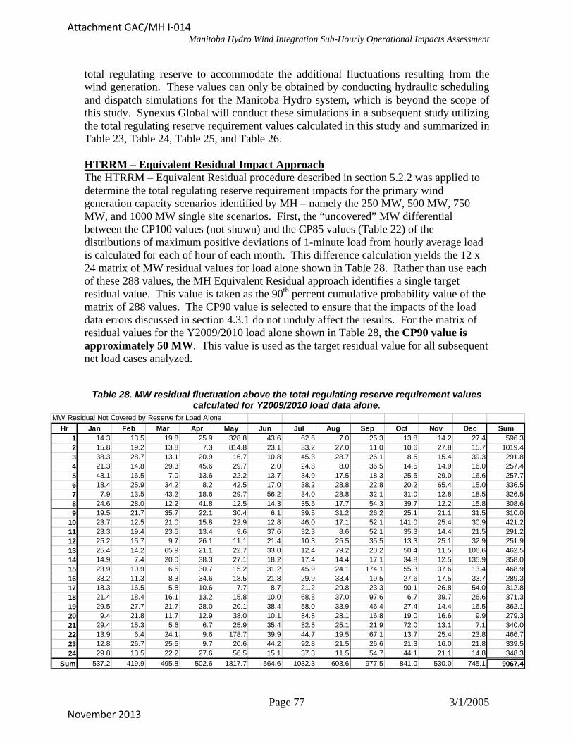
Manitoba Hydro Wind Integration Sub-Hourly Operational Impacts Assessment
total regulating reserve to accommodate the additional fluctuations resulting from the wind generation. These values can only be obtained by conducting hydraulic scheduling and dispatch simulations for the Manitoba Hydro system, which is beyond the scope of this study. Synexus Global will conduct these simulations in a subsequent study utilizing the total regulating reserve requirement values calculated in this study and summarized in Table 23, Table 24, Table 25, and Table 26.
HTRRM – Equivalent Residual Impact Approach The HTRRM – Equivalent Residual procedure described in section 5.2.2 was applied to determine the total regulating reserve requirement impacts for the primary wind generation capacity scenarios identified by MH – namely the 250 MW, 500 MW, 750 MW, and 1000 MW single site scenarios. First, the “uncovered” MW differential between the CP100 values (not shown) and the CP85 values (Table 22) of the distributions of maximum positive deviations of 1-minute load from hourly average load is calculated for each of hour of each month. This difference calculation yields the 12 x 24 matrix of MW residual values for load alone shown in Table 28. Rather than use each of these 288 values, the MH Equivalent Residual approach identifies a single target residual value. This value is taken as the 90th percent cumulative probability value of the matrix of 288 values. The CP90 value is selected to ensure that the impacts of the load data errors discussed in section 4.3.1 do not unduly affect the results. For the matrix of residual values for the Y2009/2010 load alone shown in Table 28, the CP90 value is approximately 50 MW. This value is used as the target residual value for all subsequent net load cases analyzed.
Table 28. MW residual fluctuation above the total regulating reserve requirement values calculated for Y2009/2010 load data alone.
MW Residual Not Covered by Reserve for Load Alone
Hr Jan Feb Mar Apr May Jun Jul Aug Sep Oct Nov Dec Sum1 14.3 13.5 19.8 25.9 328.8 43.6 62.6 7.0 25.3 13.8 14.2 27.4 596.32 15.8 19.2 13.8 7.3 814.8 23.1 33.2 27.0 11.0 10.6 27.8 15.7 1019.43 38.3 28.7 13.1 20.9 16.7 10.8 45.3 28.7 26.1 8.5 15.4 39.3 291.84 21.3 14.8 29.3 45.6 29.7 2.0 24.8 8.0 36.5 14.5 14.9 16.0 257.45 43.1 16.5 7.0 13.6 22.2 13.7 34.9 17.5 18.3 25.5 29.0 16.6 257.76 18.4 25.9 34.2 8.2 42.5 17.0 38.2 28.8 22.8 20.2 65.4 15.0 336.57 7.9 13.5 43.2 18.6 29.7 56.2 34.0 28.8 32.1 31.0 12.8 18.5 3268 24.6 28.0 12.2 41.8 12.5 14.3 35.5 17.7 54.3 39.7 12.2 15.8 308.69 19.5 21.7 35.7 22.1 30.4 6.1 39.5 31.2 26.2 25.1 21.1 31.5 310.0
10 23.7 12.5 21.0 15.8 22.9 12.8 46.0 17.1 52.1 141.0 25.4 30.9 421.211 23.3 19.4 23.5 13.4 9.6 37.6 32.3 8.6 52.1 35.3 14.4 21.5 291.212 25.2 15.7 9.7 26.1 11.1 21.4 10.3 25.5 35.5 13.3 25.1 32.9 251.913 25.4 14.2 65.9 21.1 22.7 33.0 12.4 79.2 20.2 50.4 11.5 106.6 462.514 14.9 7.4 20.0 38.3 27.1 18.2 17.4 14.4 17.1 34.8 12.5 135.9 35815 23.9 10.9 6.5 30.7 15.2 31.2 45.9 24.1 174.1 55.3 37.6 13.4 468.916 33.2 11.3 8.3 34.6 18.5 21.8 29.9 33.4 19.5 27.6 17.5 33.7 289.317 18.3 16.5 5.8 10.6 7.7 8.7 21.2 29.8 23.3 90.1 26.8 54.0 312.818 21.4 18.4 16.1 13.2 15.8 10.0 68.8 37.0 97.6 6.7 39.7 26.6 371.319 29.5 27.7 21.7 28.0 20.1 38.4 58.0 33.9 46.4 27.4 14.4 16.5 362.120 9.4 21.8 11.7 12.9 38.0 10.1 84.8 28.1 16.8 19.0 16.6 9.9 27921 29.4 15.3 5.6 6.7 25.9 35.4 82.5 25.1 21.9 72.0 13.1 7.1 340.022 13.9 6.4 24.1 9.6 178.7 39.9 44.7 19.5 67.1 13.7 25.4 23.8 466.723 12.8 26.7 25.5 9.7 20.6 44.2 92.8 21.5 26.6 21.3 16.0 21.8 339.524 29.8 13.5 22.2 27.6 56.5 15.1 37.3 11.5 54.7 44.1 21.1 14.8 348.3
Sum 537.2 419.9 495.8 502.6 1817.7 564.6 1032.3 603.6 977.5 841.0 530.0 745.1 9067.4
.5
.0
.3
Page 77 3/1/2005
Attachment GAC/MH I-014
November 2013

Manitoba Hydro Wind Integration Sub-Hourly Operational Impacts Assessment
With 50 MW set at the target residual value not covered by total regulating reserves, the cumulative probability percentage of maximum positive deviations of 1-minute net load from hourly average that yields a similar target residual was determined iteratively for each of the 4 wind capacity scenarios. For example, for the 250 MW single site wind generation scenario, it was determined that the 94th percent cumulative probability values of the distributions of maximum positive deviations of 1-minute net load from hourly average would yield a similar CP90 residual value of 50 MW. Table 29 shows the table of CP100 – CP94 values for the 250 MW single site case from which the CP90 of 50 MW is calculated.
Table 29. MW residual fluctuation above the total regulating reserve requirement values calculated for Y2009/2010 net load for 250 MW single site wind generation scenario.
MW Residual Not Covered by Reserve for Net Load w/ 250 MW at single site
Hr Jan Feb Mar Apr May Jun Jul Aug Sep Oct Nov Dec Sum1 23.69 6.47 19.10 24.15 270.53 11.95 33.40 19.36 12.05 23.67 31.48 6.04 481.902 55.29 5.28 19.68 40.69 771.51 39.71 22.89 23.85 20.32 3.85 15.28 27.15 1,045.513 9.86 10.45 14.38 0.81 22.93 23.18 2.17 3.75 13.02 5.53 29.83 3.99 139.924 13.55 8.69 15.66 26.62 8.48 6.76 22.02 7.95 15.70 3.70 5.40 19.17 153.705 73.48 3.28 8.08 9.26 21.15 9.78 27.28 29.07 39.65 24.08 7.89 27.92 280.916 92.67 24.41 38.25 2.41 25.37 33.31 14.19 14.52 26.84 27.34 49.96 7.32 356.587 3.81 10.80 17.61 40.21 26.42 28.16 12.31 17.99 22.08 5.65 27.25 18.50 230.808 21.74 52.78 8.59 72.90 4.63 7.96 20.54 21.25 39.41 10.85 8.46 13.75 282.879 2.05 8.49 27.53 0.99 34.54 32.99 22.37 31.05 34.77 32.87 14.47 15.53 257.65
10 34.11 8.85 27.73 12.68 7.15 12.52 19.75 42.93 37.52 112.42 26.32 35.36 377.3311 12.19 16.21 19.74 23.01 10.06 13.10 11.52 33.24 32.15 16.92 27.36 51.95 267.4512 43.33 8.32 61.55 7.94 39.62 7.11 0.97 2.99 21.77 23.27 16.79 32.60 266.2513 16.70 13.65 52.88 37.54 17.33 28.44 67.18 20.39 24.29 15.61 18.17 121.18 433.3614 16.53 11.32 10.76 23.52 12.30 7.17 34.90 21.69 7.06 30.43 14.15 116.59 306.4215 10.78 17.30 4.77 28.92 48.27 17.57 28.43 20.47 155.87 52.49 15.54 2.07 402.4916 12.92 10.31 12.05 15.00 182.42 15.63 14.61 42.50 38.82 19.80 25.38 3.25 392.7017 24.12 18.99 6.46 5.11 27.10 21.47 8.04 7.11 24.98 64.57 4.37 36.39 248.7218 18.72 24.41 21.46 17.72 7.04 10.03 60.53 6.20 69.38 7.69 28.14 8.54 279.8719 5.72 6.72 5.99 5.12 0.77 28.61 32.57 13.70 19.27 17.44 3.86 21.51 161.2820 47.52 64.45 113.20 38.21 47.19 21.74 70.47 21.15 21.40 17.61 13.77 36.49 513.2021 22.14 14.05 17.07 37.25 10.73 21.02 71.70 2.37 20.39 98.01 9.44 4.96 329.1222 12.42 8.07 144.22 25.15 169.12 9.32 7.42 31.09 13.81 20.50 8.23 10.59 459.9323 7.30 13.61 8.37 2.60 22.88 9.36 69.69 2.14 24.07 7.14 2.60 19.43 189.1824 6.73 38.54 12.92 43.60 28.74 5.70 39.43 5.98 33.84 26.55 97.31 43.03 382.35
Sum 587.4 405.5 688.1 541.4 1816.3 422.6 714.4 442.7 768.5 668.0 501.4 683.3 8239.5 A similar iterative process was followed to determine the CP percentage that yields the CP90 target residual of 50 MW for the 500 MW, 750 MW, and 1000 MW wind generation single site cases. These values are shown in Table 30.
Table 30. Cumulative probability percentages of maximum 1-minute deviations from hourly average net load that yield CP90 target residual value of 50 MW.
Wind Capacity CP Percent Yielding Target Residual
250 94% 500 98% 750 98.5% 1000 99%
Page 78 3/1/2005
Attachment GAC/MH I-014
November 2013

Manitoba Hydro Wind Integration Sub-Hourly Operational Impacts Assessment
The total regulating reserve requirement matrix for each wind generation net load capacity scenario is then calculated as the appropriate cumulative probability percentage (Table 30) of the distributions of deviations of 1-minute average net load from the corresponding hourly average value. For example, the total regulating reserve requirement values calculated for the 250 MW wind generation at 1 site case is shown in Table 31. The total regulating reserve values in Table 31 are then compared with those calculated for load alone (Table 22) to determine the incremental total regulating reserve requirement for accommodating the wind plant. Table 32 shows the additional total regulating reserve for the 250 MW single site wind capacity scenario.
Table 31. Raw total regulating reserve requirement values calculated for net load resulting from 250 MW of wind generation capacity at a single site.
Raw Total Regulating Reserve Requirement (CP94) for Net Load w/ 250 MW Wind w/1Site
Hr Jan Feb Mar Apr May Jun Jul Aug Sep Oct Nov Dec Sum1 81.94 80.92 73.98 63.88 98.12 74.89 87.58 84.85 67.39 66.65 79.26 86.89 946.352 58.49 61.08 53.26 77.83 80.97 73.02 85.69 80.29 48.11 54.77 65.93 62.17 801.603 59.74 58.59 51.57 64.85 59.82 59.37 71.83 76.41 70.88 59.88 63.15 72.92 769.014 62.41 53.23 69.96 77.40 79.02 50.12 70.95 43.90 66.13 77.35 72.58 60.08 783.125 74.27 68.99 67.27 126.32 106.57 85.63 75.40 85.44 106.40 121.77 69.96 71.44 1,059.466 140.59 118.33 141.66 162.09 165.36 152.99 148.53 133.67 169.07 181.75 107.46 114.09 1,735.577 161.78 166.82 139.01 124.60 131.34 171.26 181.92 176.50 161.15 134.11 179.01 171.48 1,898.998 116.30 96.28 105.64 89.94 130.54 89.76 128.58 116.24 123.23 97.71 127.05 137.55 1,358.829 72.92 67.47 78.41 66.79 84.16 57.42 93.38 94.51 87.90 72.16 65.02 62.18 902.32
10 82.52 69.75 67.23 73.35 65.62 68.98 91.16 81.92 64.35 71.48 97.15 57.07 890.5811 57.75 69.81 99.88 64.39 55.69 69.94 72.26 85.73 63.90 71.60 59.74 64.22 834.9112 77.50 64.06 64.93 72.81 74.96 59.09 58.83 63.67 61.26 61.14 55.58 74.98 788.8113 83.92 93.03 83.99 69.36 65.06 50.85 64.20 99.41 66.49 91.70 64.70 84.78 917.5114 74.76 66.35 48.16 81.45 75.15 83.93 47.31 55.29 60.91 80.63 50.61 69.02 793.5715 62.00 64.56 53.30 63.64 58.30 61.78 56.88 59.13 67.30 56.22 60.64 70.68 734.4316 94.31 75.62 79.90 88.33 67.84 75.26 75.24 70.20 82.93 81.20 96.37 101.89 989.0917 129.01 105.39 76.74 69.19 59.63 62.74 83.37 59.83 75.46 64.88 138.07 187.99 1,112.3018 80.79 104.85 68.59 68.74 81.71 68.44 63.93 81.36 76.53 70.56 86.95 83.80 936.2619 71.40 76.42 99.04 66.95 75.26 78.22 69.60 73.25 103.24 70.13 71.74 69.46 924.7020 65.46 64.98 60.97 94.67 98.75 69.02 70.51 81.58 67.30 59.34 68.40 68.56 869.5321 76.13 85.66 66.71 61.55 84.94 92.78 60.83 95.94 102.69 95.62 80.88 52.80 956.5122 81.89 83.51 84.37 108.47 132.23 122.40 122.42 152.68 154.35 127.59 104.19 86.33 1,360.4223 111.36 107.10 121.34 132.06 148.51 145.88 179.06 154.35 133.26 127.01 135.17 128.95 1,624.0624 149.53 116.58 118.83 105.23 106.45 124.96 131.57 123.90 96.53 94.53 131.19 145.26 1,444.56
Sum 2126.8 2019.4 1974.8 2073.9 2186.0 2048.7 2191.0 2230.0 2176.7 2089.8 2130.8 2184.6 25432.5
Page 79 3/1/2005
Attachment GAC/MH I-014
November 2013
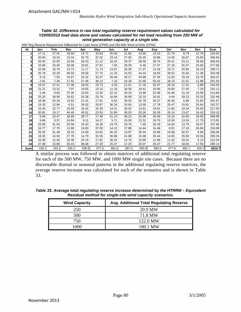
Manitoba Hydro Wind Integration Sub-Hourly Operational Impacts Assessment
Table 32. Difference in raw total regulating reserve requirement values calculated for Y2009/2010 load data alone and values calculated for net load resulting from 250 MW of
wind generation capacity at a single site. MW Reg Reserve Requirement Differential for Load Alone (CP85) and 250 MW Wind w/1Site (CP94)
Hr Jan Feb Mar Apr May Jun Jul Aug Sep Oct Nov Dec Sum1 17.11 27.01 18.59 14.71 33.63 20.56 21.82 14.95 13.15 21.79 8.79 12.79 224.912 20.94 19.24 13.34 32.70 37.02 23.14 27.55 25.45 10.86 14.09 26.67 15.83 266.843 26.00 22.05 15.69 28.43 21.12 16.42 29.37 28.58 38.75 20.41 23.12 39.99 309.934 15.69 16.40 33.08 29.81 27.81 7.56 29.59 6.46 27.07 27.18 32.37 24.65 277.665 22.06 16.79 13.72 11.17 11.73 13.67 29.39 17.27 14.18 10.71 20.80 18.23 199.716 20.78 22.29 36.50 29.58 27.70 11.25 15.52 16.44 18.63 28.52 15.50 11.36 254.087 8.15 7.55 24.67 23.32 32.57 26.46 45.27 44.88 37.04 14.29 19.19 19.70 303.078 2.91 7.26 17.91 27.45 36.12 7.10 16.18 21.68 53.42 28.13 21.51 11.88 251.549 19.97 27.41 27.06 18.03 23.73 4.20 21.01 17.18 32.97 28.19 17.42 6.89 244.05
10 21.21 13.31 7.97 16.65 13.15 11.18 34.56 19.41 19.66 24.84 27.00 7.18 216.1211 5.46 9.83 37.00 15.83 12.30 22.15 20.20 13.98 22.48 24.46 15.19 15.96 214.8412 25.20 18.06 19.62 20.38 25.76 16.84 26.68 15.10 16.91 4.44 18.13 25.33 232.4613 18.38 25.26 13.53 21.41 17.81 6.62 30.53 62.78 26.07 40.45 6.99 21.82 291.6714 24.33 12.94 6.51 26.52 26.87 36.26 10.65 13.58 17.78 25.47 15.81 25.64 242.3715 15.43 22.77 16.93 16.42 20.29 14.51 20.52 13.61 19.01 11.65 19.34 26.50 217.0016 20.81 19.17 40.40 45.51 23.50 31.80 30.03 25.26 26.39 26.14 13.67 16.43 319.1017 5.94 23.47 18.69 28.77 17.49 21.13 46.22 24.08 34.09 15.16 15.00 18.92 268.9618 6.66 9.57 24.84 9.11 14.27 5.71 15.50 21.52 19.76 15.59 13.53 17.75 173.8119 23.59 31.04 20.59 16.43 16.36 24.75 20.76 7.65 30.29 14.54 13.79 18.07 237.8620 16.77 17.75 12.80 16.83 37.00 14.12 17.88 14.44 16.46 8.91 17.19 26.83 216.9821 25.02 31.48 18.19 14.09 24.62 40.20 13.87 25.04 15.68 24.98 30.57 5.94 269.6822 18.35 14.50 27.76 14.79 31.55 30.68 41.88 15.48 35.44 14.65 25.90 19.36 290.3423 10.08 12.42 33.35 20.15 17.81 30.24 14.75 15.89 11.99 11.42 29.32 5.12 212.5424 27.48 13.89 26.43 38.48 27.33 25.47 17.25 20.07 25.47 21.77 18.94 17.55 280.13
Sum 418.3 441.5 525.2 536.6 577.5 462.0 597.0 500.8 583.6 477.8 465.7 429.7 6015.7 A similar process was followed to obtain matrices of additional total regulating reserve for each of the 500 MW, 750 MW, and 1000 MW single site cases. Because there are no discernable diurnal or seasonal patterns in the additional regulating reserve matrices, the average reserve increase was calculated for each of the scenarios and is shown in Table 33.
Table 33. Average total regulating reserve increase determined by the HTRRM – Equivalent Residual method for single-site wind capacity scenarios.
Wind Capacity Avg. Additional Total Regulating Reserve
250 20.9 MW 500 71.8 MW 750 122.0 MW 1000 180.1 MW
Page 80 3/1/2005
Attachment GAC/MH I-014
November 2013

Manitoba Hydro Wind Integration Sub-Hourly Operational Impacts Assessment
5.3 Impact on Net Load 10-Minute Fluctuations
5.3.1. General Concept The change in the system net load over a 10-minute period has several potential implications for system operators. As noted previously, the 10-minute change in system load impacts the total regulating reserves to be held by MH. Although discussed in more detail in Section 5.4, the 10-minute change in net load can contribute to increasing ACE values and possibly impact the tie line capacity that is reserved to maintain reliability margins. Additionally, the 10-minute change in system net load can have implications on contingency reserves, emergency calls to reserve sharing pools, and NERC disturbance control performance.
Without addressing these various possible implications directly, the impact of wind generation on the 10-minute change in net system load is analyzed in this section. These results may then be utilized for other impact assessment analyses such as is the case for the TRM impact analysis presented in Section 5.4.
5.3.2. Manitoba Hydro Specific Approach The probability distributions of the change in Manitoba Hydro (MH) load, wind generation, and MH system net load (load –wind generation) that occur over a 10-minute period are created. These distributions are constructed from the following data sets:
• 1-minute resolution Y2009/2010 MH system load time series synthesizedaccording to the method described in Section 5.2.2 and further described inAppendix 2.
• 1-minute resolution Y2009/2010 MH wind generation real power output timeseries for the 500 MW/1-Site scenario synthesized according to the methoddescribed in Section 5.2.2 and further described in Appendix 2.
Note that the “10-minute change” of the various quantities is determined according to two methods:
• Change in 10-min average value. The 1-minute resolution data is aggregated toyield a 10-minute average time series from which the 10-minute change isdetermined as the difference of one 10-minute average value and the previous 10-minute average value.
• Change in 1-min average value over 10-minute period. The source 1-minuteresolution time series described above are utilized to calculate the 10-minutechange as the difference in a specific 1-minute average value and the 1-minuteaverage value occurring 10 minutes prior.
5.3.3. Results and Analysis 10-Minute Change in Load Values Figure 29 shows the probability distribution of the change in MH Y2009/2010 10-minute average load. Note that the x-axis scaling is skewed to include the maximum values of –858 MW and +358 MW, which are associated with a suspicious load excursion event that occurred in the original MH load data on 5/20/03 and is represented in the synthesized
Page 81 3/1/2005
Attachment GAC/MH I-014
November 2013
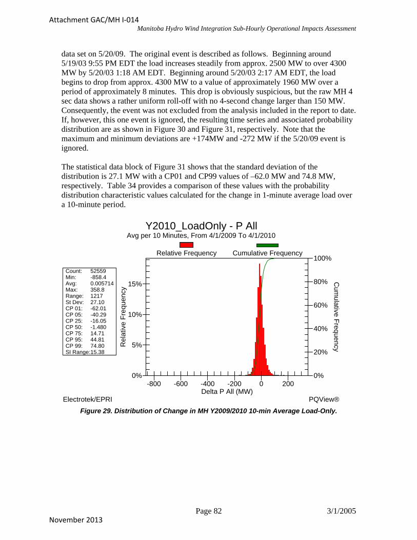
Manitoba Hydro Wind Integration Sub-Hourly Operational Impacts Assessment
data set on 5/20/09. The original event is described as follows. Beginning around 5/19/03 9:55 PM EDT the load increases steadily from approx. 2500 MW to over 4300 MW by 5/20/03 1:18 AM EDT. Beginning around 5/20/03 2:17 AM EDT, the load begins to drop from approx. 4300 MW to a value of approximately 1960 MW over a period of approximately 8 minutes. This drop is obviously suspicious, but the raw MH 4 sec data shows a rather uniform roll-off with no 4-second change larger than 150 MW. Consequently, the event was not excluded from the analysis included in the report to date. If, however, this one event is ignored, the resulting time series and associated probability distribution are as shown in Figure 30 and Figure 31, respectively. Note that the maximum and minimum deviations are +174MW and -272 MW if the 5/20/09 event is ignored. The statistical data block of Figure 31 shows that the standard deviation of the distribution is 27.1 MW with a CP01 and CP99 values of –62.0 MW and 74.8 MW, respectively. Table 34 provides a comparison of these values with the probability distribution characteristic values calculated for the change in 1-minute average load over a 10-minute period.
0%
5%
10%
15%
0%
20%
40%
60%
80%
100%
-800 -600 -400 -200 0 200
Y2010_LoadOnly - P AllAvg per 10 Minutes, From 4/1/2009 To 4/1/2010
Electrotek/EPRI PQView®
Count: 52559Min: -858.4Avg: 0.005714Max: 358.8Range: 1217St Dev: 27.10CP 01: -62.01CP 05: -40.29CP 25: -16.05CP 50: -1.480CP 75: 14.71CP 95: 44.81CP 99: 74.80SI Range:15.38
Rel
ativ
e F
requ
ency
Cum
ulative Frequency
Delta P All (MW)
Relative Frequency Cumulative Frequency
Figure 29. Distribution of Change in MH Y2009/2010 10-min Average Load-Only.
Page 82 3/1/2005
Attachment GAC/MH I-014
November 2013

Manitoba Hydro Wind Integration Sub-Hourly Operational Impacts Assessment
-300
-200
-100
0
100
200
300
May2009
Jun Jul Aug Sep Oct Nov DecJan 2010Feb Mar Apr
Y2010_LoadOnly - P AllAvg per 10 Minutes, From 4/1/2009 To 4/1/2010
Electrotek/EPRI PQView®
Del
ta P
All
(MW
)
Time
Figure 30. Time series trend of change in MH Y2009/2010 10-minute average load with
maximum excursions limited to +/- 300 MW.
0%
5%
10%
15%
0%
20%
40%
60%
80%
100%
-300 -200 -100 0 100 200
Y2010_LoadOnly - P AllAvg per 10 Minutes, From 4/1/2009 To 4/1/2010
Electrotek/EPRI PQView®
Count: 52559Min: -858.4Avg: 0.005714Max: 358.8Range: 1217St Dev: 27.10CP 01: -62.01CP 05: -40.29CP 25: -16.05CP 50: -1.480CP 75: 14.71CP 95: 44.81CP 99: 74.80SI Range:15.38
Rel
ativ
e F
requ
ency
Cum
ulative Frequency
Delta P All (MW)
Relative Frequency Cumulative Frequency
Figure 31. Probability distribution of change in MH Y2009/2010 10-minute average load with the 5/20/03 event excluded (note that data block max and min still reflect 5/20/03
event).
Page 83 3/1/2005
Attachment GAC/MH I-014
November 2013

Manitoba Hydro Wind Integration Sub-Hourly Operational Impacts Assessment
Figure 32 shows the time series trend of the change in 1-minute average load value over the previous 10-minute period. For example, the data point for 5/1/09 01:00 represents the difference in the average load values of 5/1/09 01:00 and 5/1/09 00:50. The following data point would represent the difference in the average load values of 5/1/09 01:01 and 5/1/09 00:51. Note from the time series trend of load changes in Figure 32, that the load excursion of 5/20/04 discussed previously is larger in magnitude (-1405 MW) than represented in the distribution of 10-min average load changes (-858 MW). One would expect that the change in 1-minute average values over a 10-minute period would be larger than the change in subsequent 10-minute average values as the latter introduces some degree of smoothing as part of the 10-minute average. Note also that Figure 32 also accentuates other questionable load excursion that occur on 7/28/2009, 10/21/2009, and 1/21/2010 Figure 33 and Figure 34 show the same time series trend and associated probability distribution with the maximum deviation limited to +/-300 MW. These plots allow us to better see the typical range of fluctuations on a more appropriate scale (possible data error fluctuations excluded). The statistical data block of Figure 34 shows that the standard deviation of the distribution is 33.7 MW with a CP01 and CP99 values of –77.0 MW and 86.4 MW, respectively. Table 34 provides a comparison of these values with the probability distribution characteristic values calculated for the change in 10-minute average load.
Figure 32. Time series trend of the 10-minute change in MH Y2009/2010 1-minute average
load.
Page 84 3/1/2005
Attachment GAC/MH I-014
November 2013

Manitoba Hydro Wind Integration Sub-Hourly Operational Impacts Assessment
Figure 33. Time series trend of the 10-minute change in MH Y2009/2010 1-minute average
load with maximum excursions limited to +/- 300 MW.
0%
2%
4%
6%
8%
10%
12%
14%
0%
20%
40%
60%
80%
100%
-300 -200 -100 0 100 200
Y2010_LoadOnly_10minDelta - P AllFrom 4/1/2009 To 4/1/2010
Electrotek/EPRI PQView®
Count: 525590Min: -1405Avg: 0.005714Max: 493.6Range: 1898St Dev: 33.72CP 01: -76.96CP 05: -52.18CP 25: -20.16CP 50: -1.053CP 75: 19.49CP 95: 54.78CP 99: 86.36SI Range:19.83
Rel
ativ
e F
requ
ency
Cum
ulative Frequency
P All (MW)
Relative Frequency Cumulative Frequency
Figure 34. Probability distribution of 10-minute change in MH Y2009/2010 1-minute average load with the maximum 10-minute change restricted to no more than +/-300 MW (note that
data block max and min still reflect 5/20/03 event).
Page 85 3/1/2005
Attachment GAC/MH I-014
November 2013

Manitoba Hydro Wind Integration Sub-Hourly Operational Impacts Assessment
Table 34. Comparison of probability distribution values.
Data Quantity Std. Dev. (MW)
CP01 (MW)
CP05 (MW)
CP25 (MW)
CP75 (MW)
CP95 (MW)
CP99 (MW)
Load_ ∆10minAvg 27.1 -62.0 -40.3 -16.1 14.7 44.8 74.8
Load_ 10min∆1minAvg 33.72 -77.0 -52.2 -20.2 19.5 54.8 86.4
10-Minute Change in Wind Generation Real Power Output Values Figure 35 shows the time series trend of the change in 500MW-1Site total wind plant 10-minute average real power output. The probability distribution associated with the samples comprising this time series trend is shown in Figure 36. The statistical data block of Figure 36 shows that the standard deviation of the distribution is 24.4 MW with a CP01 and CP99 values of –72.5 MW and 72.9 MW, respectively. Table 34 provides a comparison of these values with the probability distribution characteristic values calculated for the change in 1-minute average real power output over a 10-minute period.
-300
-200
-100
0
100
200
300
May2009
Jun Jul Aug Sep Oct Nov DecJan 2010Feb Mar Apr
500MW-1site - P AllAvg per 10 Minutes, From 4/1/2009 To 4/1/2010
Electrotek/EPRI PQView®
Del
ta P
All
(MW
)
Time
Figure 35. Time series trend of change in 500MW-1Site total wind plant 10-minute average
real power output.
Page 86 3/1/2005
Attachment GAC/MH I-014
November 2013

Manitoba Hydro Wind Integration Sub-Hourly Operational Impacts Assessment
0%
5%
10%
15%
20%
25%
0%
20%
40%
60%
80%
100%
-200 0 200
500MW-1site - P AllAvg per 10 Minutes, From 4/1/2009 To 4/1/2010
Electrotek/EPRI PQView®
Count: 52559Min: -362.3Avg: -0.0007605Max: 355.1Range: 717.4St Dev: 26.41CP 01: -72.48CP 05: -40CP 25: -9.587CP 50: -0.009264CP 75: 9.569CP 95: 39.69CP 99: 72.92SI Range:9.578
Rel
ativ
e F
requ
ency
Cum
ulative Frequency
Delta P All (MW)
Relative Frequency Cumulative Frequency
Figure 36. Probability distribution of change in 10-minute average real power output for a 500 MW wind plant at single site. (Note this is wind plant output only and NOT net load.)
Figure 37 shows the time series trend of the change in the 500MW-1Site total wind plant 1-minute average real power output over the previous 10-minute period. The probability distribution associated with the samples comprising this time series trend is shown in Figure 38. The statistical data block of Figure 38 shows that the standard deviation of the distribution is 28.2 MW with a CP01 and CP99 values of –79.1 MW and 79.3 MW, respectively. Table 35 provides a comparison of these values with the probability distribution characteristic values calculated for the change in 10-minute average real power output.
Page 87 3/1/2005
Attachment GAC/MH I-014
November 2013

Manitoba Hydro Wind Integration Sub-Hourly Operational Impacts Assessment
Figure 37. Time series trend of the 10-minute change in 500MW-1site 1-minute average real
power output.
0%
5%
10%
15%
20%
25%
0%
20%
40%
60%
80%
100%
-400 -200 0 200 400
500MW-1site_10minDelta - P AllFrom 4/1/2009 To 4/1/2010
Electrotek/EPRI PQView®
Count: 525590Min: -598.1Avg: -0.0007605Max: 541.4Range: 1139St Dev: 28.23CP 01: -79.08CP 05: -42.05CP 25: -10.07CP 50: -0.01069CP 75: 9.972CP 95: 42.03CP 99: 79.34SI Range:10.02
Rel
ativ
e F
requ
ency
Cum
ulative Frequency
P All (MW)
Relative Frequency Cumulative Frequency
Figure 38. Probability distribution of the 10-minute change in 500MW-1site 1-minute
average real power output.
Page 88 3/1/2005
Attachment GAC/MH I-014
November 2013

Manitoba Hydro Wind Integration Sub-Hourly Operational Impacts Assessment
Table 35. Comparison of 500MW/1Site real power output change probability distribution values.
Data Quantity Std. Dev. (MW)
CP01 (MW)
CP05 (MW)
CP25 (MW)
CP75 (MW)
CP95 (MW)
CP99 (MW)
Wg_ ∆10minAvg 26.4 -72.5 -40.0 -9.6 9.6 39.7 72.9
Wg_ 10min∆1minAvg 28.2 -79.1 -42.05 -10.1 10.0 42.0 79.3
10-Minute Change in Net Load Values Figure 39 shows the time series trend of the change in MH Y2009/2010 10-minute average net load where the 500 MW – 1 site total wind plant real power output is considered a negative load. Note that the suspicious 5/20/09 load excursion event is apparent in the net load change trend just as with the system load change trend. If this one event is ignored, the resulting time series and associated probability distribution are as shown in Figure 40 and Figure 41, respectively. Note that the maximum and minimum deviations are +407 MW and -269 MW if the 5/20/09 event is ignored.
The statistical data block of Figure 41 shows that the standard deviation of the distribution is 38.0 MW with a CP01 and CP99 values of –93.0 MW and 98.1 MW, respectively. Table 36 provides a comparison of these values with the probability distribution characteristic values calculated for the change in 1-minute average net load over a 10-minute period.
-800
-600
-400
-200
0
200
400
May2009
Jun Jul Aug Sep Oct Nov DecJan 2010Feb Mar Apr
NetLoad_Y2010-500MW_1Site - P AllAvg per 10 Minutes, From 4/1/2009 To 4/1/2010
Electrotek/EPRI PQView®
Del
ta P
All
(MW
)
Time
Figure 39. Time series trend in change in 10-minute average system net load for a 500 MW
wind plant at single site.
Page 89 3/1/2005
Attachment GAC/MH I-014
November 2013
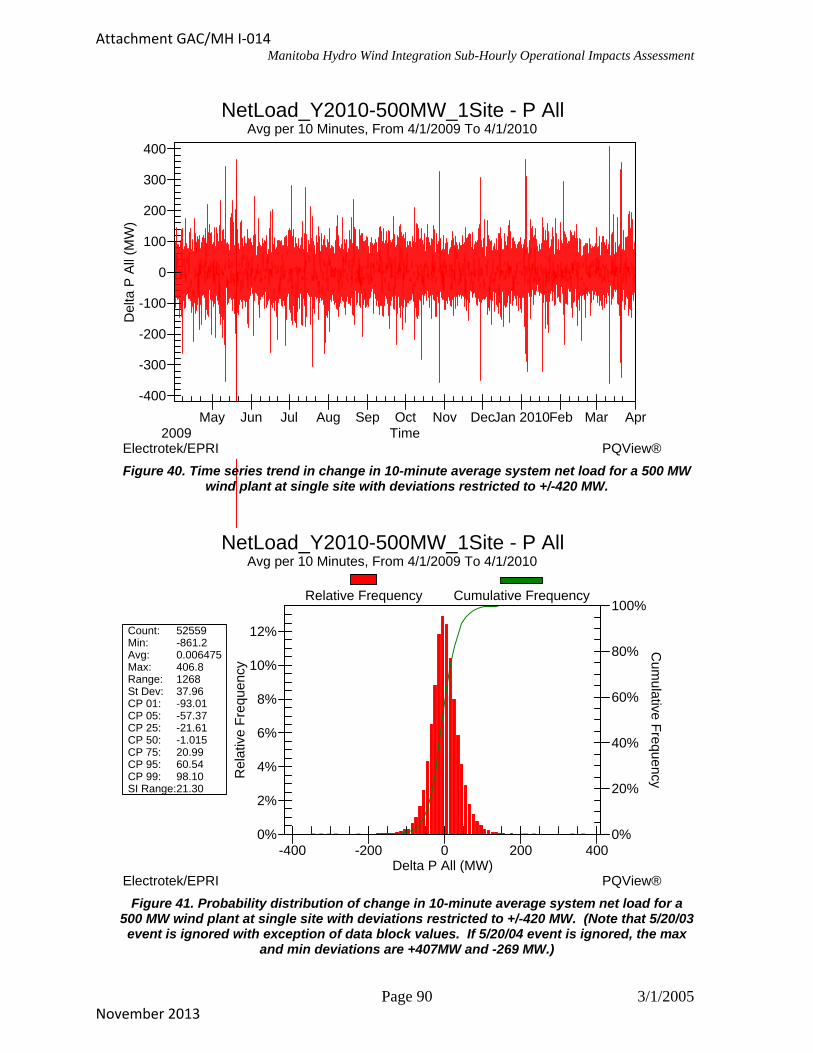
Manitoba Hydro Wind Integration Sub-Hourly Operational Impacts Assessment
-400
-300
-200
-100
0
100
200
300
400
May2009
Jun Jul Aug Sep Oct Nov DecJan 2010Feb Mar Apr
NetLoad_Y2010-500MW_1Site - P AllAvg per 10 Minutes, From 4/1/2009 To 4/1/2010
Electrotek/EPRI PQView®
Del
ta P
All
(MW
)
Time
Figure 40. Time series trend in change in 10-minute average system net load for a 500 MW
wind plant at single site with deviations restricted to +/-420 MW.
0%
2%
4%
6%
8%
10%
12%
0%
20%
40%
60%
80%
100%
-400 -200 0 200 400
NetLoad_Y2010-500MW_1Site - P AllAvg per 10 Minutes, From 4/1/2009 To 4/1/2010
Electrotek/EPRI PQView®
Count: 52559Min: -861.2Avg: 0.006475Max: 406.8Range: 1268St Dev: 37.96CP 01: -93.01CP 05: -57.37CP 25: -21.61CP 50: -1.015CP 75: 20.99CP 95: 60.54CP 99: 98.10SI Range:21.30
Rel
ativ
e F
requ
ency
Cum
ulative Frequency
Delta P All (MW)
Relative Frequency Cumulative Frequency
Figure 41. Probability distribution of change in 10-minute average system net load for a
500 MW wind plant at single site with deviations restricted to +/-420 MW. (Note that 5/20/03 event is ignored with exception of data block values. If 5/20/04 event is ignored, the max
and min deviations are +407MW and -269 MW.)
Page 90 3/1/2005
Attachment GAC/MH I-014
November 2013

Manitoba Hydro Wind Integration Sub-Hourly Operational Impacts Assessment
Figure 42 shows the time series trend of the change in 1-minute average load value over the previous 10-minute period. For example, the data point for 5/1/09 01:00 represents the difference in the average net load values of 5/1/09 01:00 and 5/1/09 00:50. The following data point would represent the difference in the average load values of 5/1/09 01:01 and 5/1/09 00:51. Note that the suspicious 5/20/09 load excursion event is apparent in the net load change trend just as with the other trends/distributions that include a component of the load change. If this one event is ignored, the resulting time series and associated probability distribution are as shown in Figure 43 and Figure 44, respectively. The statistical data block of Figure 44 shows that the standard deviation of the distribution is 44.1 MW with a CP01 and CP99 values of –106.8 MW and 111.7 MW, respectively. Table 36 provides a comparison of these values with the probability distribution characteristic values calculated for the change in 10-minute average load.
Page 91 3/1/2005
Attachment GAC/MH I-014
November 2013

Manitoba Hydro Wind Integration Sub-Hourly Operational Impacts Assessment
Figure 42. Time series trend in change in 1-minute average system net load (500 MW wind plant at single site) occurring over a 10-minuter period.
Figure 43. Time series trend in change in 1-minute average system net load (500 MW wind plant at single site) occurring over a 10-minuter period with deviations limited to +/- 600
MW.
Page 92 3/1/2005
Attachment GAC/MH I-014
November 2013

Manitoba Hydro Wind Integration Sub-Hourly Operational Impacts Assessment
0%
2%
4%
6%
8%
10%
0%
20%
40%
60%
80%
100%
-600 -400 -200 0 200 400
NetLoad_10minDelta_Y2010_500MW_1Site - P AllFrom 4/1/2009 To 4/1/2010
Electrotek/EPRI PQView®
Count: 525590Min: -1414Avg: 0.006475Max: 607Range: 2021St Dev: 44.12CP 01: -106.8CP 05: -67.44CP 25: -25.82CP 50: -0.7714CP 75: 25.42CP 95: 70.07CP 99: 111.7SI Range:25.62
Rel
ativ
e F
requ
ency
Cum
ulative Frequency
P All (MW)
Relative Frequency Cumulative Frequency
Figure 44. Probability distribution of change in 1-minute average system net load (500 MW wind plant at single site) occurring over a 10-minuter period with deviations limited to +/-
600 MW.
Table 36. Comparison of net load (500MW/1Site) change probability distribution values.
Data Quantity Std. Dev. (MW)
CP01 (MW)
CP05 (MW)
CP25 (MW)
CP75 (MW)
CP95 (MW)
CP99 (MW)
NetLoad_ ∆10minAvg 38.0 -93.0 -57.4 -21.6 21.0 60.5 98.1
NetLoad_ 10min∆1minAvg 44.1 -106.8 -67.4 -25.8 25.42 70.1 111.7
Analysis of 10-Minute Change in Net Load Values Table 37 provides a comparison of the probability distribution characteristics for the 10-minute changes in load, wind generation, and net load calculated for each of the two 10-minute change methods.
Table 37. Comparison of statistical distributions for 10-minute changes in load, wind generation, and net load for the 500 MW – 1-Site scenario.
Data Quantity Std. Dev. (MW)
CP01 (MW)
CP05 (MW)
CP25 (MW)
CP75 (MW)
CP95 (MW)
CP99 (MW)
Load_ ∆10minAvg 27.1 -62.0 -40.3 -16.1 14.7 44.8 74.8
Wg_ ∆10minAvg 26.4 -72.5 -40.0 -9.6 9.6 39.7 72.9
NetLoad_ ∆10minAvg 38.0 -93.0 -57.4 -21.6 21.0 60.5 98.1
Load_ 10min∆1minAvg 33.7 -77.0 -52.2 -20.2 19.5 54.8 86.4 Wg_ 10min∆1minAvg 28.2 -79.1 -42.1 -10.1 10.0 42.0 79.3 NetLoad_ 10min∆1minAvg 44.1 -106.8 -67.4 -25.8 25.42 70.1 111.7
Page 93 3/1/2005
Attachment GAC/MH I-014
November 2013

Manitoba Hydro Wind Integration Sub-Hourly Operational Impacts Assessment
First, note from Table 37 that the standard deviation of the net load change distribution increases approximately 10-11 MW relative to the distribution of change in load alone for both the distributions of 10-min average change (38.0 MW to 27.1 MW) and change in 1-min average over 10-minute period (44.1 MW to 33.7 MW). These increases are almost exactly predicted by assuming that the correlation between the load and wind generation changes is totally uncorrelated. This assumption was confirmed by calculating the correlation coefficient between a subset of the two time series (approximately 1 month of data) yielding a correlation coefficient of approximately 0.02.
Secondly, note that the CP01 and CP99 values also increase by a similar percentage with the CP01 increasing from –62.0 MW to –93.0 MW and the CP99 increasing from 74.8 MW to 98.1 MW for the 10-minute average. Similarly, the CP01 increases from –77.0 MW to –106.8 MW and the CP99 increases from 86.4 MW to 111.7 MW for the change in 1-minute average over a 10-minute period.
Figure 45 and Figure 46 provide further insights as to how the tails of the 10-minute net load fluctuation distributions are impacted with increasing wind generation levels. Figure 45 shows the trend in the 99%, 99.5%, and 99.9% cumulative probability values of the distribution of 10-minute change in the 1-minute average net load for various wind generation capacity scenarios ranging from no wind to 1400 MW of wind at a single site. These trends provide an idea as to the magnitude of the most extreme positive net load changes (where extremity refers to those changes occurring 1% of the time or less) that can be expected. Notice that as the wind generation capacity increases, the increase in a given CP value accelerates. This is because the fluctuations in wind generation output are more volatile than the fluctuations in system load when considered on a per unit basis. Because the relative magnitude of system load is large relative to the smaller wind generation capacities, the impacts on net load fluctuations are relatively small as the fluctuations of the wind generation output are swamped by the fluctuations of the large system load quantity. For example, although the CP99 value for the 250 MW wind plant 10-minute fluctuations is approximately 14% of the maximum wind plant output and the comparable system load value is only 2%, the impact of the 250 MW wind plant on the net system load CP99 value is small, with the net load CP99 value increasing 8.5% from 86.35 MW to 93.75 MW. As the wind penetration level increases to a level comparable to the magnitude of system peak load, the wind generation fluctuations contribute more to total net load fluctuations, eventually dominating the total fluctuations. This can be seen in Figure 45 where the CP99 value for the 1400MW net load scenario is approximately 2.5 times greater than for system load alone.
Figure 45 also shows that the acceleration of the increase of the CP value is more pronounced for more extreme CP values. Note that the 99.9% CP curve accelerates much more quickly than the CP99 curve. This is because the wind plant is increasingly more volatile at the extremes of the distribution than the system load on a per unit basis. Thus, the wind generation fluctuations more significantly influence net system load fluctuation CP values more quickly.
Page 94 3/1/2005
Attachment GAC/MH I-014
November 2013

Manitoba Hydro Wind Integration Sub-Hourly Operational Impacts Assessment
0.00
50.00
100.00
150.00
200.00
250.00
300.00
350.00
400.00
450.00
500.00
Load Only NetLd-250MW
NetLd-500MW
NetLd-750MW
NetLd-1000MW
NetLd-1400MW
Wind Cap. Scenario
MW
Ch
ang
e
CP-99.9%
CP-99.5%
CP-99.0%
Figure 45. Comparison of the extreme positive values of the cumulative probability
function for the 10-minute change in 1-minute average net load for various wind capacity scenarios.
Figure 46 shows the trend in the 0.1%, 0.5%, and 1.0% cumulative probability values of the distribution of 10-minute change in the 1-minute average net load for various wind generation capacity scenarios ranging from no wind to 1400 MW of wind at a single site. These trends provide an idea as to the magnitude of the most extreme negative net load changes (where extremity refers to those changes occurring 1% of the time or less) that can be expected. Figure 46 shows very similar trends in the extremities of the negative fluctuations as seen in the positive fluctuations from Figure 45:
1. Increase in a given CP value accelerates with wind penetration level 2. Acceleration rate in CP value is higher for more extreme CP values
Table 38 shows the percentage increase in the extreme 10-minute net load fluctuation cumulative probability function values for various wind capacity levels.
Page 95 3/1/2005
Attachment GAC/MH I-014
November 2013

Manitoba Hydro Wind Integration Sub-Hourly Operational Impacts Assessment
-500.00
-450.00
-400.00
-350.00
-300.00
-250.00
-200.00
-150.00
-100.00
-50.00
0.00
Load Only NetLd-250MW
NetLd-500MW
NetLd-750MW
NetLd-1000MW
NetLd-1400MW
Wind Cap. Scenario
MW
Ch
ang
e
CP-1.0%
CP-0.5%
CP-0.1%
Figure 46. Comparison of the extreme negative values of the cumulative probability function for the 10-minute change in 1-minute average net load for various wind capacity
scenarios.
Table 38. Percent increase in net load 10-minute fluctuation cumulative probability values for various single site wind capacity levels.
NetLd-250MW NetLd-500MW NetLd-750MW NetLd-1000MWNetLd-1400MWCP-99.9% 8.03% 36.43% 80.41% 130.12% 212.75%CP-99.5% 8.69% 31.04% 64.04% 103.51% 171.37%CP-99.0% 8.57% 29.40% 59.76% 95.96% 159.21%CP-1.0% 11.51% 38.71% 75.88% 118.79% 192.61%CP-0.5% 12.25% 42.97% 86.27% 134.68% 215.65%CP-0.1% 15.53% 60.58% 121.98% 184.73% 291.71%
Page 96 3/1/2005
Attachment GAC/MH I-014
November 2013

Manitoba Hydro Wind Integration Sub-Hourly Operational Impacts Assessment
5.4 Transmission Reliability Margin (TRM)
5.4.1. General Approach Transmission reliability margin (TRM) is the portion of the transmission transfer capability that is reserved to provide a safety margin to accommodate uncertainties in the transmission system. Such uncertainties potentially include facility outages and load uncertainties17, 18. Integrating significant wind generation into a given control area introduces additional uncertainty, and therefore, may impact TRM.
AGC is intended to regulate load variations on a minute-by-minute time scale. The additional total regulating reserve required to accommodate the fluctuations of wind generation on a minute to several minute time frame is addressed in the high-frequency regulation impact assessment (section 5.1) and load following impact assessment (section 5.2). Depending on the quality of the total regulating reserves allocated and the tuning of the AGC parameters, some portion of the 1-10 minute fluctuations in system net load will still impact ACE. Furthermore, sub-minute fluctuations may not be controlled by AGC at all. Consequently, system operators may have to hold back some MW amount of the tie line capability for conducting transactions. This holdback would represent a component of TRM to support the uncontrolled 1-10 minute and sub-minute fluctuations of the tie-line flows that occur in response to instantaneous variations of the load for different control areas of the interconnection. As wind generation is added to a control area, the 1-10 minute and sub-minute fluctuations of wind generation will increase the overall fluctuation of the system such that additional transmission reliability margin may be required.
Manitoba Hydro does not currently reserve additional TRM to accommodate the fluctuations of system net load. Thus the primary question to be answered is whether wind generation significantly impacts the magnitude of the sub-minute and multi-minute fluctuations of net load (load minus wind generation). To this end, a simple two-fold approach is taken. First, the standard deviation of the distribution of sub-minute fluctuations calculated and is utilized as an assessment metric to determine the relative magnitude impact on sub-minute fluctuations. Secondly, the distribution of 10-minute changes in load, wind generation, and net load presented in Section 5.3 are considered to assess the relative magnitude increase in these longer term changes, a portion of which might show up on the ties. These approaches are not intended to yield the exact value of TRM to be withheld, but rather to assess whether the change in the magnitude and frequency of fluctuations that might impact tie line flows is significant enough to warrant holding additional TRM to accommodate net load fluctuations.
5.4.2. Specific Manitoba Hydro Assessment Method The sub-minute fluctuation of system load is calculated from the historical 4-second EMS data as the deviation of the 4-second resolution time series data with respect to the
17 MAPP Regional Transmission Reliability Margin Methodology, January 11, 2001. 18 Manitoba Hydro Internal Document – “Manitoba U.S. Interface Operating Guidelines.”
Page 97 3/1/2005
Attachment GAC/MH I-014
November 2013

Manitoba Hydro Wind Integration Sub-Hourly Operational Impacts Assessment
corresponding 1-minute average values. As for the regulation assessment, the method utilized to scale the sub-minute fluctuation component of system load for the future study year is based on the assumption that fluctuations between individual loads are uncorrelated. As such, the standard deviation of the future year sub-minute fluctuation distribution is obtained by scaling the base case year fluctuation series by the square root of ratio of the future year hourly average load and reference year hourly average load. The following steps describe the exact procedure of processing the 4-second resolution system load data of year 2003/2004.
1. Calculate the 1-minute moving average time series for the base 4-secondresolution EMS archive data. The resulting moving average time series is also a4-second resolution series with the value of a given time point, t, calculated as theaverage of values of the base 4-second resolution time series that fall within thewindow of t-30 seconds to t+30 seconds.
2. Calculate the sub-minute fluctuation time series by subtracting the original 4-second resolution time series by the 1-minute moving average time series.
3. It is assumed that the fluctuations of system load at a 4-second resolution arestatistically uncorrelated. As such, this component of the total system load scalesaccording to the square root of the ratio of total system load for the new and basecase scenarios. Thus, for the TRM analysis, each data point of the Y2003/Y2004load sub-minute fluctuation series is scaled by the square root of the ratio of thecorresponding hourly average load values for Y2009/2010 and Y2003//2004 asshown in Equation 7.
i
i
HR
HRii L
LLfLf
04/2003
10/200904/200310/2009 ×= Equation 7
where,
Lfi ≡ load fluctuation for 4-sec resolution point i LHRi ≡ hourly average load corresponding to clock hour of 4-sec resolution
fluctuation point i
The 4-second wind generation fluctuation series is also obtained in a very similar manner as for the regulation assessment. As noted in section 4.3.2, there is no historical high-resolution wind generation or wind speed measurement data for the proposed Manitoba wind sites. As such, 1-second resolution wind generation data from wind plant at Buffalo Ridge area of Minnesota is used as a surrogate to obtain a 4-second resolution data for three wind plants. This base data set is then used to extract the sub-minute fluctuation of wind generation from the total high-resolution data set using a procedure similar to that described for the load. As with the high-resolution load data, this source wind generation fluctuation distribution must be altered to reflect the desired study year scenarios. Unlike the load data, however, we do not assume any growth pattern for the wind resource. Rather, the study year scenarios to be analyzed require that we obtain high-resolution fluctuation series for each of the Manitoba sites for several different wind plant capacity
Page 98 3/1/2005
Attachment GAC/MH I-014
November 2013

Manitoba Hydro Wind Integration Sub-Hourly Operational Impacts Assessment
levels that differ from the capacity levels represented by the source data measurements. Thus, for each of the different wind plant capacity allocations, the source data fluctuation series must be scaled to represent the desired scenario capacity allocations. As noted previously, it is assumed that the high-frequency fluctuations for turbines within the same plant are statistically uncorrelated. As such, the model utilized to obtain the wind generation fluctuation series for the various capacity allocations is as follows:
Assuming that the fluctuation of wind generation output at a 4-second resolution is statistically uncorrelated, this sub-minute fluctuation series of the total wind generation output for a given capacity level scales according to the square root of the ratio of total capacity for the new and base case scenarios. Thus, each data point of the Y2003/Y2004 wind generation sub-minute fluctuation series for any one of the 3 sites is scaled by the square root of the ratio of the desired wind plant capacity and the source date capacity value as shown in Equation 8.
base
newii Wcap
WcapbaseWfnewWf ×−=− Equation 8
where,
Wfi ≡ wind generation fluctuation for 4-second resolution point i Wcap ≡ total wind plant capacity for scenario or measurement series
Due to the volume of 4-second data points comprised by a full year of data and the higher number of samples contained within a smaller assessment period, the TRM assessment is conducted utilizing the fluctuation series for high and low wind generation and system load weeks. Because the fluctuations of load and wind generation are assumed to be statistically uncorrelated, the one-week time series selected for load and the various wind plants do not have to be coincident in time. As such, the peak load and minimum load weeks were selected, as well as a high- and low-wind week for each of the three wind plants. The actual time periods selected for each quantity and the average hourly value of the quantity over the period are shown in Table 39.
Table 39. Summary of load and wind generation periods selected for TRM assessment. High Period Low Period
Quantity Date Range Hr Avg (MW) Date Range Hr Avg (MW)) MH Load 1/22/2004 -
1/29/2004 3390 7/8/2003 -
7/15/2003 2023
St. Leon (Plant #1)
3/8/2004 - 3/15/2004
124.0 (230 MW rated)
8/8/2003 - 8/15/2003
31.1 (230 MW rated)
Minnedosa (Plant #2B)
3/8/2004 - 3/15/2004
37.7 (66 MW rated)
6/8/2003 - 6/15/2003
10.9 (66 MW rated)
Boissevain (Plant #2A)
3/8/2004 - 3/15/2004
26.6 (47 MW rated)
6/8/2003 - 6/15/2003
6.9 (47 MW rated)
Page 99 3/1/2005
Attachment GAC/MH I-014
November 2013

Manitoba Hydro Wind Integration Sub-Hourly Operational Impacts Assessment
The standard deviations of the system load and wind generation sub-minute fluctuation series for the selected period are converted to the same period for the various study year capacity scenarios according to the procedures stated above. For each study year capacity scenario, the standard deviation of the net system load is then obtained by further assuming that high-frequency fluctuations of load and wind generation are uncorrelated. Under this assumption, the standard deviation of the aggregate fluctuation of wind and load is calculated as the square root of the sum of the squares of standard deviations of load and wind generation as shown in Equation 9.
22WindLoadNetLoad σσσ += Equation 9
where,
σNetLoad ≡ standard deviation of aggregate load and wind fluctuation σLoad ≡ standard deviation of load fluctuation σWind ≡ standard deviation of wind fluctuation
The standard deviation of the aggregate fluctuation is then used to determine the relative increase in the sub-minute fluctuation resulting from integrating the various wind scenarios. This impact is calculated as the percent increase of the aggregate standard deviation over the standard deviation for the load alone (no wind generation scenario).
5.4.3. Results and Analysis The procedure described in the previous section was performed for all of the study year wind capacity scenarios for the four combinations of high/low load and wind generation samples. Figure 47 shows the study year load sub-minute fluctuation probability distribution. This distribution shows that during the peak load week, 98% of the sub-minute fluctuations of the load alone are contained within a band of –19.0 MW to +18.2 MW, with the most extreme fluctuations ranging from –49.2 MW to 57.5 MW. The standard deviation of the distribution is 7.34 MW. The distribution characteristics for the low-load period are very similar with the variations slightly smaller as expected – 98% of variations within a band of –14.2 MW and 13.9 MW and a standard deviation of 5.67 MW.
Page 100 3/1/2005
Attachment GAC/MH I-014
November 2013

Manitoba Hydro Wind Integration Sub-Hourly Operational Impacts Assessment
0%
5%
10%
15%
20%
25%
0%
20%
40%
60%
80%
100%
-40 -20 0 20 40
Y2009/2010 Load Sub-Minute FluctuationHigh-Load Period (1/22/2010 - 1/29/2010)
Electrotek/EPRI PQView®
Count: 151198Min: -49.19Avg: 0.00004672Max: 57.52Range: 106.7St Dev: 7.340CP 01: -19.04CP 05: -12.01CP 25: -4.414CP 50: 0.05048CP 75: 4.503CP 95: 11.78CP 99: 18.19SI Range:4.459
Rel
ativ
e F
requ
ency
Cum
ulative Frequency
P All (MW)
Relative Frequency Cumulative Frequency
Figure 47. Sub-minute load fluctuation probability distribution for Y2003/2004 high-load period.
Figure 48 shows the total wind generation sub-minute fluctuation probability distribution for the high-wind period for the 500 MW capacity uniformly distributed between 2 sites. This distribution is oddly shaped because of the relative small fluctuation magnitude of most samples compared to the large magnitude of 2 samples. As a result, the bin size required to span all of the sample magnitudes is so large that all but a couple sample fall within 2 bins. It should be noted that the 2 large magnitude deviation samples are the result of a significant drop in wind generation output in the source Plant #1 data. These drops appear to be the result of 1 or more collection strings within the wind plant dropping out due to some protection action. Despite these two large non-wind related events, the distribution shows that the during the high-wind period, 98% of the sub-minute fluctuations of the load alone are contained within a band of –1.9 MW to +1.9 MW. The standard deviation of the distribution is 0.88 MW.
Page 101 3/1/2005
Attachment GAC/MH I-014
November 2013
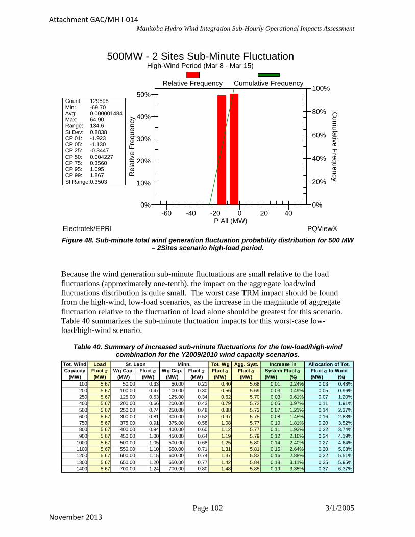
Manitoba Hydro Wind Integration Sub-Hourly Operational Impacts Assessment
0%
10%
20%
30%
40%
50%
0%
20%
40%
60%
80%
100%
-60 -40 -20 0 20 40
500MW - 2 Sites Sub-Minute FluctuationHigh-Wind Period (Mar 8 - Mar 15)
Electrotek/EPRI PQView®
Count: 129598Min: -69.70Avg: 0.000001484Max: 64.90Range: 134.6St Dev: 0.8838CP 01: -1.923CP 05: -1.130CP 25: -0.3447CP 50: 0.004227CP 75: 0.3560CP 95: 1.095CP 99: 1.867SI Range:0.3503
Rel
ativ
e F
requ
ency
Cum
ulative Frequency
P All (MW)
Relative Frequency Cumulative Frequency
Figure 48. Sub-minute total wind generation fluctuation probability distribution for 500 MW
– 2Sites scenario high-load period.
Because the wind generation sub-minute fluctuations are small relative to the load fluctuations (approximately one-tenth), the impact on the aggregate load/wind fluctuations distribution is quite small. The worst case TRM impact should be found from the high-wind, low-load scenarios, as the increase in the magnitude of aggregate fluctuation relative to the fluctuation of load alone should be greatest for this scenario. Table 40 summarizes the sub-minute fluctuation impacts for this worst-case low-load/high-wind scenario.
Table 40. Summary of increased sub-minute fluctuations for the low-load/high-wind combination for the Y2009/2010 wind capacity scenarios.
Tot. Wind Load Tot. Wg Agg. Syst.Capacity Fluct σ Wg Cap. Fluct σ Wg Cap. Fluct σ Fluct σ Fluct σ
(MW) (MW) (MW) (MW) (MW) (MW) (MW) (MW) (MW) (%) (MW) (%)100 5.67 50.00 0.33 50.00 0.21 0.40 5.68 0.01 0.24% 0.03 0.48%200 5.67 100.00 0.47 100.00 0.30 0.56 5.69 0.03 0.49% 0.05 0.96%250 5.67 125.00 0.53 125.00 0.34 0.62 5.70 0.03 0.61% 0.07 1.20%400 5.67 200.00 0.66 200.00 0.43 0.79 5.72 0.05 0.97% 0.11 1.91%500 5.67 250.00 0.74 250.00 0.48 0.88 5.73 0.07 1.21% 0.14 2.37%600 5.67 300.00 0.81 300.00 0.52 0.97 5.75 0.08 1.45% 0.16 2.83%750 5.67 375.00 0.91 375.00 0.58 1.08 5.77 0.10 1.81% 0.20 3.52%800 5.67 400.00 0.94 400.00 0.60 1.12 5.77 0.11 1.93% 0.22 3.74%900 5.67 450.00 1.00 450.00 0.64 1.19 5.79 0.12 2.16% 0.24 4.19%
1000 5.67 500.00 1.05 500.00 0.68 1.25 5.80 0.14 2.40% 0.27 4.64%1100 5.67 550.00 1.10 550.00 0.71 1.31 5.81 0.15 2.64% 0.30 5.08%1200 5.67 600.00 1.15 600.00 0.74 1.37 5.83 0.16 2.88% 0.32 5.51%1300 5.67 650.00 1.20 650.00 0.77 1.42 5.84 0.18 3.11% 0.35 5.95%1400 5.67 700.00 1.24 700.00 0.80 1.48 5.85 0.19 3.35% 0.37 6.37%
Allocation of Tot.Fluct σ to Wind
St. Leon Minn. Increase inSystem Fluct σ
Page 102 3/1/2005
Attachment GAC/MH I-014
November 2013
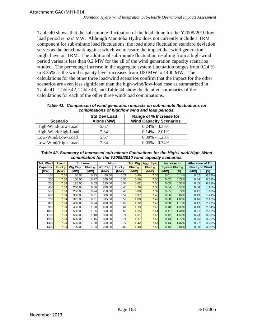
Manitoba Hydro Wind Integration Sub-Hourly Operational Impacts Assessment
Table 40 shows that the sub-minute fluctuation of the load alone for the Y2009/2010 low-load period is 5.67 MW. Although Manitoba Hydro does not currently include a TRM component for sub-minute load fluctuations, the load alone fluctuation standard deviation serves as the benchmark against which we measure the impact that wind generation might have on TRM. The additional sub-minute fluctuation resulting from a high-wind period varies is less than 0.2 MW for the all of the wind generation capacity scenarios studied. The percentage increase in the aggregate system fluctuation ranges from 0.24 % to 3.35% as the wind capacity level increases from 100 MW to 1400 MW. The calculations for the other three load/wind scenarios confirm that the impact for the other scenarios are even less significant than the high-wind/low-load case as summarized in Table 41. Table 42, Table 43, and Table 44 show the detailed summaries of the calculations for each of the other three wind/load combinations.
Table 41. Comparison of wind generation impacts on sub-minute fluctuations for combinations of high/low wind and load periods.
Scenario Std Dev Load Alone (MW)
Range of % Increase for Wind Capacity Scenarios
High-Wind/Low-Load 5.67 0.24% - 3.35% High-Wind/High-Load 7.34 0.14% - 2.01% Low-Wind/Low-Load 5.67 0.09% - 1.23% Low-Wind/High-Load 7.34 0.05% - 0.74%
Table 42. Summary of increased sub-minute fluctuations for the High-Load/ High -Wind combination for the Y2009/2010 wind capacity scenarios.
Tot. Wind Load Tot. Wg Agg. Syst.Capacity Fluct σ Wg Cap. Fluct σ Wg Cap. Fluct σ Fluct σ Fluct σ
(MW) (MW) (MW) (MW) (MW) (MW) (MW) (MW) (MW) (%) (MW) (%)100 7.34 50.00 0.33 50.00 0.21 0.40 7.35 0.01 0.14% 0.02 0.29%200 7.34 100.00 0.47 100.00 0.30 0.56 7.36 0.02 0.29% 0.04 0.58%250 7.34 125.00 0.53 125.00 0.34 0.62 7.36 0.03 0.36% 0.05 0.72%400 7.34 200.00 0.66 200.00 0.43 0.79 7.38 0.04 0.58% 0.08 1.15%500 7.34 250.00 0.74 250.00 0.48 0.88 7.39 0.05 0.72% 0.11 1.43%600 7.34 300.00 0.81 300.00 0.52 0.97 7.40 0.06 0.87% 0.13 1.71%750 7.34 375.00 0.91 375.00 0.58 1.08 7.42 0.08 1.08% 0.16 2.13%800 7.34 400.00 0.94 400.00 0.60 1.12 7.42 0.08 1.15% 0.17 2.27%900 7.34 450.00 1.00 450.00 0.64 1.19 7.43 0.10 1.30% 0.19 2.54%
1000 7.34 500.00 1.05 500.00 0.68 1.25 7.44 0.11 1.44% 0.21 2.82%1100 7.34 550.00 1.10 550.00 0.71 1.31 7.45 0.12 1.58% 0.23 3.09%1200 7.34 600.00 1.15 600.00 0.74 1.37 7.46 0.13 1.72% 0.25 3.36%1300 7.34 650.00 1.20 650.00 0.77 1.42 7.47 0.14 1.87% 0.27 3.63%1400 7.34 700.00 1.24 700.00 0.80 1.48 7.48 0.15 2.01% 0.29 3.90%
Allocation of Tot.Fluct σ to Wind
St. Leon Minn. Increase inSystem Fluct σ
Page 103 3/1/2005
Attachment GAC/MH I-014
November 2013

Manitoba Hydro Wind Integration Sub-Hourly Operational Impacts Assessment
Table 43. Summary of increased sub-minute fluctuations for the Low-Load/Low-Wind combination for the Y2009/2010 wind capacity scenarios.
Tot. Wind Load Tot. Wg Agg. Syst.Capacity Fluct σ Wg Cap. Fluct σ Wg Cap. Fluct σ Fluct σ Fluct σ
(MW) (MW) (MW) (MW) (MW) (MW) (MW) (MW) (MW) (%) (MW) (%)100 5.67 50.00 0.10 50.00 0.21 0.24 5.67 0.01 0.09% 0.01 0.18%200 5.67 100.00 0.15 100.00 0.30 0.34 5.68 0.01 0.18% 0.02 0.35%250 5.67 125.00 0.17 125.00 0.34 0.38 5.68 0.01 0.22% 0.03 0.44%400 5.67 200.00 0.21 200.00 0.43 0.48 5.69 0.02 0.35% 0.04 0.70%500 5.67 250.00 0.23 250.00 0.48 0.53 5.69 0.03 0.44% 0.05 0.88%600 5.67 300.00 0.26 300.00 0.53 0.58 5.70 0.03 0.53% 0.06 1.05%750 5.67 375.00 0.29 375.00 0.59 0.65 5.70 0.04 0.66% 0.07 1.31%800 5.67 400.00 0.30 400.00 0.61 0.67 5.71 0.04 0.71% 0.08 1.40%900 5.67 450.00 0.31 450.00 0.64 0.72 5.71 0.05 0.80% 0.09 1.57%
1000 5.67 500.00 0.33 500.00 0.68 0.75 5.72 0.05 0.88% 0.10 1.74%1100 5.67 550.00 0.35 550.00 0.71 0.79 5.72 0.06 0.97% 0.11 1.91%1200 5.67 600.00 0.36 600.00 0.74 0.83 5.72 0.06 1.06% 0.12 2.08%1300 5.67 650.00 0.38 650.00 0.77 0.86 5.73 0.06 1.15% 0.13 2.25%1400 5.67 700.00 0.39 700.00 0.80 0.89 5.73 0.07 1.23% 0.14 2.42%
Allocation of Tot.Fluct σ to Wind
St. Leon Minn. Increase inSystem Fluct σ
Table 44. Summary of increased sub-minute fluctuations for the High-Load/Low-Wind combination for the Y2009/2010 wind capacity scenarios.
Tot. Wind Load Tot. Wg Agg. Syst.Capacity Fluct σ Wg Cap. Fluct σ Wg Cap. Fluct σ Fluct σ Fluct σ
(MW) (MW) (MW) (MW) (MW) (MW) (MW) (MW) (MW) (%) (MW) (%)100 7.34 50.00 0.10 50.00 0.21 0.24 7.34 0.00 0.05% 0.01 0.11%200 7.34 100.00 0.15 100.00 0.30 0.34 7.34 0.01 0.11% 0.02 0.21%250 7.34 125.00 0.17 125.00 0.34 0.38 7.35 0.01 0.13% 0.02 0.26%400 7.34 200.00 0.21 200.00 0.43 0.48 7.35 0.02 0.21% 0.03 0.42%500 7.34 250.00 0.23 250.00 0.48 0.53 7.36 0.02 0.26% 0.04 0.53%600 7.34 300.00 0.26 300.00 0.53 0.58 7.36 0.02 0.32% 0.05 0.63%750 7.34 375.00 0.29 375.00 0.59 0.65 7.37 0.03 0.40% 0.06 0.79%800 7.34 400.00 0.30 400.00 0.61 0.67 7.37 0.03 0.42% 0.06 0.84%900 7.34 450.00 0.31 450.00 0.64 0.72 7.37 0.03 0.47% 0.07 0.94%
1000 7.34 500.00 0.33 500.00 0.68 0.75 7.37 0.04 0.53% 0.08 1.05%1100 7.34 550.00 0.35 550.00 0.71 0.79 7.38 0.04 0.58% 0.08 1.15%1200 7.34 600.00 0.36 600.00 0.74 0.83 7.38 0.05 0.63% 0.09 1.25%1300 7.34 650.00 0.38 650.00 0.77 0.86 7.39 0.05 0.69% 0.10 1.36%1400 7.34 700.00 0.39 700.00 0.80 0.89 7.39 0.05 0.74% 0.11 1.46%
Allocation of Tot.Fluct σ to Wind
St. Leon Minn. Increase inSystem Fluct σ
As Table 41 shows, the impact of even high penetration wind generation scenarios on the sub-minute fluctuations is quite small with the worst case scenario showing a 3.35% increase in the standard deviation of the net load sub-minute fluctuation distribution. Thus, it is unlikely that additional TRM would be required only on the basis of the impact on sub-minute fluctuations that might flow on the tie lines.
Analysis of a small subset of MH interchange data values indicates that some portion of the longer trending (10-minute) of MH load changes are coupled into the tie line interchange. As such, the previous analysis of impacts of wind generation on MH TRM based on the increased intra-minute fluctuation of the net system load likely does not completely represent the impacts that wind generation might have on TRM. Comparison of the changes in load relative to net load with the 500 MW/1-site wind plant for both methods from Table 37 indicates that the 10-minute fluctuations in wind plant real power output will increase the standard deviation and middle quartiles of the 10-minute net load fluctuations on the order of 25%-33%. The 500 MW of wind generation will increase the extreme (CP01 and CP99) 10-minute net load fluctuations on the order of 30%-50%. Furthermore, Table 38 shows that for higher penetration levels, the extremities of the net
Page 104 3/1/2005
Attachment GAC/MH I-014
November 2013

Manitoba Hydro Wind Integration Sub-Hourly Operational Impacts Assessment
load 10-minute change distribution spread even further with the CP01 and CP99 values increasing by a factor of 2-3 and the CP0.1 and CP99.9 values increasing by a factor of 2-4. The extent to which any of these fluctuations actually flow on the tie lines isdependent on the quality of total regulating reserves maintained and on the tuning of the AGC algorithm. If AGC is tuned to perfectly control generation to track net load changes on the order of several minutes, none of the 10-minute fluctuations will show on the ties. If, however, AGC is tuned to control more loosely, some portion of the fluctuations may show on the ties. Table 38 shows that the absolute worst case scenario of no control of 10-minute fluctuations, the flows on the ties resulting from these flows would increase on the order of 1.5-3 times. Based on discussions with MH personnel and internal analysis of a small set of tie line flow data, it is expected that given the current AGC tuning, a relatively small portion of the total 10-minute changes will actually flow on the ties. MH system operators will have to make a decision as to whether the increased tie line flows on might warrant reserving tie line capacity.
Page 105 3/1/2005
Attachment GAC/MH I-014
November 2013

Manitoba Hydro Wind Integration Sub-Hourly Operational Impacts Assessment
6. ConclusionsThis study has focused on the assessment of certain sub-hourly operational impacts ofintegrating wind generation into the Manitoba Hydro control area, as well as the synthesisof wind generation and system load time series to support other evaluations being madeas part of the overall MH wind integration assessment effort. The primary products ofthis study are as follows:
• Synthesis of hourly wind generation time series for use in hourly resolutionsimulations using MH’s short-term hydraulic planning tool.
• Sensitivity analysis of impacts of varying wind speed time series and generationsynthesis algorithms on wind plant energy production and real power fluctuations(evaluation of originally synthesized wind generation time series relative to windgeneration time series synthesized from Helimax adjusted wind speed data).
• Processing of NREL 1-second wind plant real power output data as a proxy forconducting the high-frequency regulation impact analysis.
• Synthesis of Manitoba 1-minute resolution wind generation and system load timeseries for the Y2009/2010 study year for the total regulating reserve impactanalysis and other evaluations conducted as part of the larger MH windintegration impact assessment effort.
• Assessment of the impact of various wind generation capacity scenarios rangingfrom 100 MW to 1400 MW on the high-frequency regulating reserve requirement.
• Assessment of the impact of various wind generation capacity scenarios rangingfrom 100 MW to 1400 MW on MH’s total regulating reserve requirement ascalculated for MH’s current method and an extension of this method.
• Analysis of the impact on 10-minute changes in system net load for various windcapacity scenarios ranging from 250 MW to 1400 MW.
• Assessment of the potential TRM impact to accommodate the fluctuations in netsystem load that might result in additional tie-line flows.
6.1 Wind Generation Time Series Synthesis Hourly resolution wind generation time series were synthesized for 3 projected Manitoba wind plants based on metrological data collected at the 3 Manitoba sites. The approach utilized to synthesize the projected wind plant real power output time series is based on using a steady-state wind turbine generator power curve with the single mast metrological time series data. Adjustments are made for height differentials, air density, and various losses. The algorithm utilized is simple relative to meso-scale numeric weather prediction based approaches, but yields reasonable results that include the full range of variability of wind plant output needed to assess potential impacts. In general, the approach utilized yields power fluctuations that are more severe than seen in an actual wind plant, primarily because the model does not represent the full extent of intra-plant diversity that exists in actual wind plants. This results in steeper ramp rates and increased fluctuations, which provided a slightly conservative result when assessing the impacts of wind generation on net load variability.
Page 106 3/1/2005
Attachment GAC/MH I-014
November 2013

Manitoba Hydro Wind Integration Sub-Hourly Operational Impacts Assessment
Due to differences in the wind generation estimation approach, the hourly time series synthesis performed for this study yielded slightly higher (42.3% vs. 38.9% for St. Leon) net capacity factors than were calculated in a parallel study performed by Helimax. Comparison of the two separate approaches shows that there are several factors that result in this difference in calculated energy yield, with the primary factor being the lack of direct treatment of wake losses in the approach utilized in this study. In further analysis and comparison of the outputs of the two approaches, it was verified that inclusion of a treatment of wake losses provided net capacity factor results that were within 1%. It was also shown that the impacts of relatively slight variations in the source meteorological data to produce a more representative “wind year” did not significantly impact the real power fluctuations obtained from the wind plants. With the confidence provided by these validation analyses, the hourly resolution wind plant time series were approved as inputs to the subsequent Synexus Global short-term hydraulic operations planning simulation study.
In addition to the hourly resolution wind generation time series, 4-second and 1-minute resolution time series were required for integration impact assessment activities. These higher resolution time series were obtained by utilizing proxy data of actual wind plant output measurements obtained from NREL. The higher-resolution fluctuations inherent in this proxy data were isolated and scaled appropriately to represent the fluctuations of wind plants of the desired rated capacities utilized in the study scenarios. These scaled high-resolution fluctuations were then superimposed onto other appropriately scaled smoother variation components of the synthesized hourly resolution data from the projected Manitoba sites. This process yielded 1-minute and 4-second resolution wind generation time series for various wind capacity scenarios needed to analyze various potential wind integration impacts, including the high-frequency regulating reserve impacts and total regulating reserve impact analyses conducted as part of this study. Similar processes were utilized to obtain 1-minute resolution load time series for the future study year based on load growth estimate provided by Manitoba Hydro.
6.2 High-Frequency Regulation Impact The 1-minute resolution wind generation and system load time series data for the projected wind plant capacities and future study year were utilized to assess the impact of wind generation on the high-frequency regulating reserve requirement for tracking the minute-to-minute variations in net load and maintaining the desired NERC compliance. The approach utilized for the assessment is based on the decomposition of system net load into a high-frequency fluctuation component and a slower varying ramping component. The intent of the decomposition is to allow quantification of the reserve required for system regulation. A fundamental assumption underlying this approach is that on-line units are re-dispatched every 5-10 minutes to follow longer-term ramping of system net load. As such, the regulating reserve requirement would be associated with the high-frequency variations. Manitoba Hydro does not operate their predominantly hydro system in this manner, but rather they attempt to bring additional hydro units on-line at optimal generating points to most efficiently utilize available water. As such, MH maintains total regulating reserves, comprising both spinning and non-spinning capacity, for tracking high-frequency fluctuations and longer-term ramping of system net load. As
Page 107 3/1/2005
Attachment GAC/MH I-014
November 2013

Manitoba Hydro Wind Integration Sub-Hourly Operational Impacts Assessment
such, the high-frequency regulating reserve impact assessment does not represent the total impact to MH’s regulating reserve burden, but rather represents only the impact to the portion of Manitoba Hydro’s total regulating reserve requirement that is utilized to track the minute-to-minute, random variations in system net load.
The analysis conducted shows that the integration of wind generation ranging in capacity from 100 MW to 1400 MW would increase the high-frequency regulating reserve requirement 1.5% - 11% above that for system load alone (see Table 17). A key assumption of the analytical approach was that the high-frequency fluctuation in output of wind turbines within the same wind plant is statistically uncorrelated. This is assumption is not completely accurate as there is a small, positive correlation between the output of turbines within close proximity. Sensitivity analysis of the high-frequency impact results to the within-plant correlation assumptions show that the impacts calculated for the 0% correlation assumption may double if an exaggerated intra-plant correlation level is assumed. Even with these unrealistic correlation levels, the impact on high-frequency regulation requirements for the highest penetration scenario of 1400 MW at a single site is an increase of approximately 10 MW above that required for load alone, or approximately a 20% increase (see Table 19).
6.3 Total Regulating Reserve Requirement Impact The 1-minute resolution wind generation and system load time series data for the projected wind plant capacities and future study year were also utilized to assess the impact of wind generation on Manitoba Hydro’s total regulating reserve requirement. This total regulating reserve requirement comprises both spinning and non-spinning capacity and is maintained for tracking high-frequency fluctuations and longer-term ramping of system net load. The approach implemented to quantify this impact is based on Manitoba Hydro’s internal total regulating reserve requirement calculation. The currently utilized method is referred to as the Hourly Total Regulating Reserve Method –CP85 (HTRRM – CP85). This method allocates reserves to cover 85% of the maximum variations of 4-second load from the corresponding hourly average for each clock hour of the day in each calendar month. This approach results in a 12 x 24 matrix of total regulating reserve requirement values calculated from at least one year of historical data. The first quantification of the impact of wind generation on total regulating reserve requirement utilized this HTRRM-CP85 method to calculate the reserve matrix for load alone and for system net load for each of the 23 wind capacity scenarios, with the impact determined as the increase in the total regulating reserve requirement. The average impact on any given hour was found to range from 9 MW – 69 MW for wind generation capacities of 250 MW – 1000 MW at a single site.
In reviewing the adequacy of the current HTRRM – CP85 method under increasing wind penetration levels, it was recognized that the probability of relatively large changes in net load increase rapidly as wind penetration levels increase as a percentage of system peak load. The HTRRM – CP85 method does not capture the impact of the larger reserve deficits associated with these more extreme net load changes or the potential for associated degradation of NERC performance criteria. Furthermore, Manitoba Hydro noted that it might have to alter its current operating procedures so as to ensure that the
Page 108 3/1/2005
Attachment GAC/MH I-014
November 2013

Manitoba Hydro Wind Integration Sub-Hourly Operational Impacts Assessment
magnitudes of inadvertent interchanges with its tie-line neighbors do not significantly increase and to maintain NERC control performance criteria at existing levels. Consequently, an extension of the current HTRRM method was utilized to assess the additional reserve required to maintain a specified MW magnitude differential between the reserve value and the largest anticipated fluctuation magnitude (HTRRM-Equivalent Residual) as compared to the current criteria of expected percent of the time for which the magnitude of fluctuations exceeds reserves. Consequently, the impact on total regulating reserve requirement was also assessed as the additional reserves as calculated from the extended HTRRM -Equivalent Residual method to provide a range of potential impacts. This method yielded an average impact on even given hour in the range of 21 MW – 180 MW for wind generation capacities of 250 MW – 1000 MW at a single site. The higher calculated values using the HTRRM – Equivalent Residual method result from the fact that extreme deviations in wind plant output are more probable on a per unit basis than load deviations. The HTRRM – Equivalent Residual method focuses on the extremities of the net load deviation probability distributions where the integration of wind generation pushes these extremities out farther than it does the more central portions of the distributions such as the CP85 point.
6.4 Analysis of 10-Minute Changes in Net Load The probability distributions of the change in Manitoba Hydro (MH) load, wind generation, and MH system net load (load –wind generation) that occur over a 10-minute period were created. These distributions are constructed from the 1-minute resolution Y2009/2010 MH system load and projected wind plant real power output time series. The “10-minute change” of the various quantities was determined according to two methods:
• Change in 10-min average value. The 1-minute resolution data is aggregated toyield a 10-minute average time series from which the 10-minute change isdetermined as the difference of one 10-minute average value and the previous 10-minute average value.
• Change in 1-min average value over 10-minute period. The source 1-minuteresolution time series described above are utilized to calculate the 10-minutechange as the difference in a specific 1-minute average value and the 1-minuteaverage value occurring 10 minutes prior.
It was found that the addition of wind increases the probability of occurrence of the most significant net load changes. For example, the magnitude of the 10-minute net load change that is expected 99% of the time increases by a factor of 2 for 1000 MW of wind and by a factor of 2.5 for 1400 MW of wind. All of these results are summarized in Table 37 and Table 38.
The change in the system net load over a 10-minute period has several potential implications for system operators. As noted previously, the 10-minute change in system load impacts the total regulating reserves to be held by MH. Although discussed in more detail in Section 5.4, the 10-minute change in net load can contribute to increasing ACE values and possibly impact the tie line capacity that is reserved to maintain reliability
Page 109 3/1/2005
Attachment GAC/MH I-014
November 2013
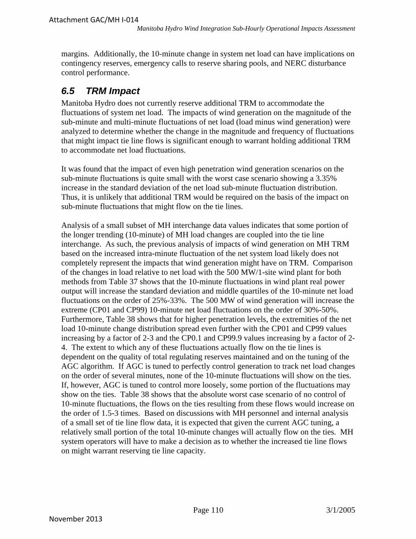
Manitoba Hydro Wind Integration Sub-Hourly Operational Impacts Assessment
margins. Additionally, the 10-minute change in system net load can have implications on contingency reserves, emergency calls to reserve sharing pools, and NERC disturbance control performance.
6.5 TRM Impact Manitoba Hydro does not currently reserve additional TRM to accommodate the fluctuations of system net load. The impacts of wind generation on the magnitude of the sub-minute and multi-minute fluctuations of net load (load minus wind generation) were analyzed to determine whether the change in the magnitude and frequency of fluctuations that might impact tie line flows is significant enough to warrant holding additional TRM to accommodate net load fluctuations.
It was found that the impact of even high penetration wind generation scenarios on the sub-minute fluctuations is quite small with the worst case scenario showing a 3.35% increase in the standard deviation of the net load sub-minute fluctuation distribution. Thus, it is unlikely that additional TRM would be required on the basis of the impact on sub-minute fluctuations that might flow on the tie lines.
Analysis of a small subset of MH interchange data values indicates that some portion of the longer trending (10-minute) of MH load changes are coupled into the tie line interchange. As such, the previous analysis of impacts of wind generation on MH TRM based on the increased intra-minute fluctuation of the net system load likely does not completely represent the impacts that wind generation might have on TRM. Comparison of the changes in load relative to net load with the 500 MW/1-site wind plant for both methods from Table 37 shows that the 10-minute fluctuations in wind plant real power output will increase the standard deviation and middle quartiles of the 10-minute net load fluctuations on the order of 25%-33%. The 500 MW of wind generation will increase the extreme (CP01 and CP99) 10-minute net load fluctuations on the order of 30%-50%. Furthermore, Table 38 shows that for higher penetration levels, the extremities of the net load 10-minute change distribution spread even further with the CP01 and CP99 values increasing by a factor of 2-3 and the CP0.1 and CP99.9 values increasing by a factor of 2-4. The extent to which any of these fluctuations actually flow on the tie lines isdependent on the quality of total regulating reserves maintained and on the tuning of the AGC algorithm. If AGC is tuned to perfectly control generation to track net load changes on the order of several minutes, none of the 10-minute fluctuations will show on the ties. If, however, AGC is tuned to control more loosely, some portion of the fluctuations may show on the ties. Table 38 shows that the absolute worst case scenario of no control of 10-minute fluctuations, the flows on the ties resulting from these flows would increase on the order of 1.5-3 times. Based on discussions with MH personnel and internal analysis of a small set of tie line flow data, it is expected that given the current AGC tuning, a relatively small portion of the total 10-minute changes will actually flow on the ties. MH system operators will have to make a decision as to whether the increased tie line flows on might warrant reserving tie line capacity.
Page 110 3/1/2005
Attachment GAC/MH I-014
November 2013
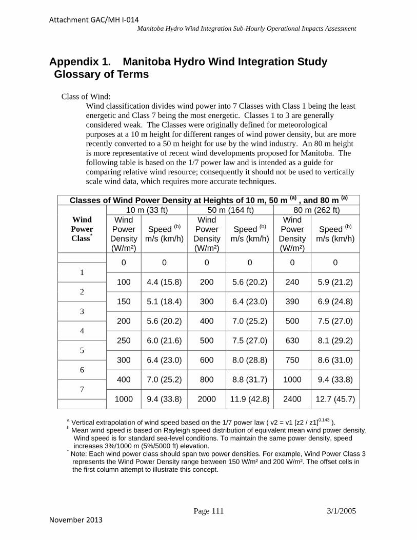
Manitoba Hydro Wind Integration Sub-Hourly Operational Impacts Assessment
Appendix 1. Manitoba Hydro Wind Integration Study Glossary of Terms
Class of Wind: Wind classification divides wind power into 7 Classes with Class 1 being the least energetic and Class 7 being the most energetic. Classes 1 to 3 are generally considered weak. The Classes were originally defined for meteorological purposes at a 10 m height for different ranges of wind power density, but are more recently converted to a 50 m height for use by the wind industry. An 80 m height is more representative of recent wind developments proposed for Manitoba. The following table is based on the 1/7 power law and is intended as a guide for comparing relative wind resource; consequently it should not be used to vertically scale wind data, which requires more accurate techniques.
Classes of Wind Power Density at Heights of 10 m, 50 m (a) , and 80 m (a) 10 m (33 ft) 50 m (164 ft) 80 m (262 ft)
Wind Power Class*
Wind Power Density (W/m²)
Speed (b) m/s (km/h)
Wind Power Density (W/m²)
Speed (b) m/s (km/h)
Wind Power Density (W/m²)
Speed (b) m/s (km/h)
0 0 0 0 0 01
100 4.4 (15.8) 200 5.6 (20.2) 240 5.9 (21.2) 2
150 5.1 (18.4) 300 6.4 (23.0) 390 6.9 (24.8) 3
200 5.6 (20.2) 400 7.0 (25.2) 500 7.5 (27.0) 4
250 6.0 (21.6) 500 7.5 (27.0) 630 8.1 (29.2) 5
300 6.4 (23.0) 600 8.0 (28.8) 750 8.6 (31.0) 6
400 7.0 (25.2) 800 8.8 (31.7) 1000 9.4 (33.8) 7
1000 9.4 (33.8) 2000 11.9 (42.8) 2400 12.7 (45.7)
a Vertical extrapolation of wind speed based on the 1/7 power law ( v2 = v1 [z2 / z1]0.143 ). b Mean wind speed is based on Rayleigh speed distribution of equivalent mean wind power density.
Wind speed is for standard sea-level conditions. To maintain the same power density, speed increases 3%/1000 m (5%/5000 ft) elevation.
* Note: Each wind power class should span two power densities. For example, Wind Power Class 3represents the Wind Power Density range between 150 W/m² and 200 W/m². The offset cells inthe first column attempt to illustrate this concept.
Page 111 3/1/2005
Attachment GAC/MH I-014
November 2013

Manitoba Hydro Wind Integration Sub-Hourly Operational Impacts Assessment
Control Area: An electrical system bounded by interconnection (tie-line) metering and telemetry. A control area controls the generation within its geographic boundaries directly to maintain its interchange schedules with other control areas and contributes to the frequency control of the region. Manitoba Hydro, Saskpower and Ontario are each separate control areas.
Contingency Reserve: Generation capacity set aside to cover contingencies on the bulk electric system, such as the loss of generation units or transmission lines. The amount of contingency reserve is determined by reliability organizations in accordance with NERC criteria. Contingency Reserves are generally specified as a mix of spinning and non-spinning (also called supplemental) generation.
CPS 1 and 2: Control Performance Standards 1 and 2 as specified NERC Policy 1 – Generation Control and Performance. Each control area must monitor its control area performance against these two standards. These Control Performance Standards establish the statistical boundaries for variations which ensure that the steady-state system frequency variations are acceptable. They are a measure of how well a control area balances load and generation within its boundaries.
Dispatchable A resource is dispatchable if it the generation level can be changed in response to changes in loading conditions.
Load Following Component: Involves the deployment of generation resources to track the demand pattern over the course of the day. It covers the adjustments required to compensate for changes in the control area demand as the load transitions through the daily load pattern. The load following component may be provided by spinning or non-spinning generation.
NERC: NORTH AMERICAN ELECTRIC RELIABILITY COUNCIL
Regulation Component: Occurs on a very short time scale (minute to minute) and involves automatic control of a sufficient amount of generating capacity to support frequency control and maintain scheduled transactions with other control areas. May also be called the high frequency regulation component. These fast changes can be thought of as the temporary ups and downs around a longer term (hourly) load following pattern. The regulation component is generally provided by spinning reserve generation placed on AGC (Automatic Generation Control).
Page 112 3/1/2005
Attachment GAC/MH I-014
November 2013

Manitoba Hydro Wind Integration Sub-Hourly Operational Impacts Assessment
Schedule: The planned interchange of power between two adjacent control areas. Each transaction is scheduled, typically on an hourly basis, and the control areas operators maintain the supply and demand balance within their control areas considering any scheduled flows between them. For example a 100 MW export from Manitoba to Saskatchewan is a 100 MW schedule, that results in the Manitoba Hydro control area over generating by 100 MW and the Saskatchewan control area under generating by 100 MW.
Spinning Reserve: A type of operating reserve that is provided by a generator synchronized to the electrical system and is capable and is available to serve load within a few minutes. All of the regulation component, plus a portion of the load following component and contingency reserves are provided by spinning reserve.
Total Regulation Reserve: Equals Regulation Component plus the Load Following Component
Total Operating Reserve: Equals the Total Regulation Reserve plus the Contingency Reserve. In general, operating reserve represents the capability above firm system demand required to provide regulation, load forecasting error, equipment forced and scheduled outages, and other capacity requirements.
TRM: Transmission Reliability Margin – The amount of transmission transfer capability necessary to ensure that the interconnected transmission network is secure under a reasonable range of uncertainties in system conditions.
Unit Commitment and Scheduling: Operations planning activities aimed at developing the lowest cost plan for meeting the forecast control area demand for the next day or days. For predominately thermal systems, this involves the starting up or “commitment” of sufficient thermal units up to 36 hours before the operating hour to ensure the units is available to meet the peak load. Such early start up of thermal units is required due to the slow ramping capability of thermal units (particularly coal units), and results in additional fuel costs. Predominately thermal systems with significant amounts of wind may require the commitment of thermal units to provide standby thermal generation capacity to cover against the loss of wind generation.
For predominately thermal systems, such unit commitment decisions are analyzed at the planning level by operation and market simulation software such as Henwood’s Prosym or New Energies ProModIV. For a predominately hydro system, the equivalent analysis is done using hydraulic operations planning and analysis tools. The MOST software developed by Synexus Global of Niagara Falls is one such hydraulic operations planning and analysis tool.
Page 113 3/1/2005
Attachment GAC/MH I-014
November 2013

Manitoba Hydro Wind Integration Sub-Hourly Operational Impacts Assessment
Appendix 2. Detailed Description of Y2009/2010 1-Minute Load and Wind Generation Time Series Synthesis Method
A2.1 Load Series Synthesis First, we consider the synthesis of the Y2009/2010 1-minute resolution system load time series. The objective is to synthesize the 1-minute resolution system load time series from April 1, 2009 through March 31, 2010. In the following detailed description, this period is called the target period. The period from April 1, 2003 to March 31, 2004 for which the base measured data was obtained is called the historical data period.
Source input data include:
• Hourly load time series for the historical data period (Ld_2004_hr).• Hourly load time series for the target period (Ld_2010_hr).• Minute-resolution system load time series for the historical data period
(Ld_2004_1min).
Detailed Synthesis Procedure:
1. First, using the Oak Ridge approach discussed in section 5.1.1, the 30-minutemoving average of the Y2003/2004 system load time series (Ld_2004_1min) iscalculated yielding a 1-minute resolution slow varying component(Ld_2004_1min_30Mov).
2. Taking the difference between Ld_2004_1min and Ld_2004_1min_30Mov, theY2003/3004 1-minute resolution minute-by-minute system load high frequencyfluctuation time series is obtained (Ld_2004_1min_Fluct).
3. An hourly load ratio time series (Ld_Ratio_hr) is obtained by dividing theY2009/2010 hourly load (Ld_2010_hr) by the corresponding hourly values of theY2003/2004 hourly load (Ld_2004_hr).
4. The Y2009/2010 1-minute resolution minute-by-minute system load highfrequency fluctuation time series (Ld_2010_1min_Fluct) is obtained by scalingLd_2004_1min_Fluct by the square root of the corresponding hourly system loadratio from Ld_Ratio_Hr. Using the square root of the ratio is based on theassumption that high frequency fluctuations between individual loads arestatistically uncorrelated.
5. The Y2003/2004 1-minute resolution time series for smooth ramping betweenhourly average loads of successive hours (Ld_2004_1min_InterHrRamp) isobtained from a process whereby the slopes of two linear segments aredetermined to preserve the hourly energy between Ld_2004_1min_30Mov andLd_2004_1min_InterHrRamp. Methodology is developed for this process wherethe trajectory of Ld_2004_1min_InterHrRamp consists of linear segments. Thetrajectory is continuous between hours and within hour. Each hour consists ofexactly 2 linear segments.
Page 114 3/1/2005
Attachment GAC/MH I-014
November 2013

Manitoba Hydro Wind Integration Sub-Hourly Operational Impacts Assessment
6. The Y2003/2004 intra-hour slow varying fluctuation of load with respect to theinter-hour smooth ramping (Ld_2004_1min_InterHrRamp) is obtained bysubtracting Ld_2004_1min_30Mov by Ld_2004_1min_InterHrRamp. Theresulting time series is denoted as Ld_2004_1min_IntraHrFluct.
7. The Y2009/2010 1-minute resolution time series for smooth ramping betweenhourly average loads of successive hours (Ld_2010_1min_InterHrRamp) isobtained from a process whereby the hourly energy is preserved betweenLd_2010_hr and Ld_2010_1min_InterHrRamp. The 1-minute-resolution timeseries Ld_2010_1min_InterHrRamp has the same characteristic asLd_2004_1min_InterHrRamp described in step 5 as the same methodologydeveloped in step 5 is used for this calculation.
8. The Y2009/2010 1-minute resolution time series of intra-hour slow varyingfluctuation of system load with respect to the inter-hour smooth ramping(Ld_2010_1min_IntraHrFluct) is obtained by scaling
Ld_2004_1min_IntraHrFluct by the scaling factor, ( )( ) 5.021 xx ⋅+⋅− ρρ , whereρ is the correlation coefficient of intra-hour fluctuations between two differentindividual loads and x is the corresponding hourly system load ratio fromLd_Ratio_Hr. It is assumed that the correlation coefficient is the same for anypair of individual loads. A correlation coefficient value of 0.5 is assumed as theintra-hour fluctuation is of a time resolution that is known to exhibit a correlationvalue between 0 and 1. Thus, the mid-point is assumed as an approximation.
9. The desired Y2009/2010 1-minute resolution system load (Ld_2010_1min) isobtained by summing the three synthesized individual component seriesLd_2010_1min_InterHrRamp, Ld_2010_1min_IntraHrFluct andLd_2010_1min_Fluct.
A2.2 Wind Generation Series Synthesis We next consider the synthesis of 1-minute resolution wind generation time series of wind capacity.
In Manitoba Hydro study project, 3 wind sites with different project levels of wind plant capacity for each site are considered. However, without loss of any generality, the description which follows considers the synthesis of wind generation for a wind sites of a given wind plant capacity. Extension to multi wind sites and multi levels of wind capacities for each wind site is trivial.
The objective is to synthesis the 1-minute resolution wind generation time series for a given site with a given projected wind plant capacity. The time period for which wind generation synthesis is performed is from April 1, 2003 to March 31, 2004. We call this time period the synthesis period. Wind speed measurement on 10-minute average for this period was collected for the site.
Input data for the synthesis process include:
Page 115 3/1/2005
Attachment GAC/MH I-014
November 2013
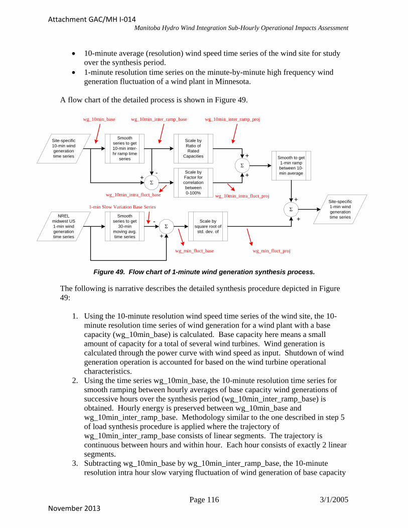
Manitoba Hydro Wind Integration Sub-Hourly Operational Impacts Assessment
• 10-minute average (resolution) wind speed time series of the wind site for studyover the synthesis period.
• 1-minute resolution time series on the minute-by-minute high frequency windgeneration fluctuation of a wind plant in Minnesota.
A flow chart of the detailed process is shown in Figure 49.
Site-specific10-min windgenerationtime series
Smoothseries to get10-min inter-hr ramp time
series
Scale byRatio ofRated
Capacities
Σ+
- Scale byFactor forcorrelationbetween0-100%
Σ
+
+ Smooth to get1-min rampbetween 10-min average
NRELmidwest US1-min windgenerationtime series
Smoothseries to get
30-minmoving avg.time series
Σ
+
- Scale bysquare root of
std. dev. of
Σ
+
+
Site-specific1-min windgenerationtime series
wg_10min_base wg_10min_inter_ramp_base wg_10min_inter_ramp_proj
wg_10min_intra_fluct_base wg_10min_intra_fluct_proj
1-min Slow Variation Base Series
wg_min_fluct_base wg_min_fluct_proj
Figure 49. Flow chart of 1-minute wind generation synthesis process.
The following is narrative describes the detailed synthesis procedure depicted in Figure 49:
1. Using the 10-minute resolution wind speed time series of the wind site, the 10-minute resolution time series of wind generation for a wind plant with a basecapacity (wg_10min_base) is calculated. Base capacity here means a smallamount of capacity for a total of several wind turbines. Wind generation iscalculated through the power curve with wind speed as input. Shutdown of windgeneration operation is accounted for based on the wind turbine operationalcharacteristics.
2. Using the time series wg_10min_base, the 10-minute resolution time series forsmooth ramping between hourly averages of base capacity wind generations ofsuccessive hours over the synthesis period (wg_10min_inter_ramp_base) isobtained. Hourly energy is preserved between wg_10min_base andwg_10min_inter_ramp_base. Methodology similar to the one described in step 5of load synthesis procedure is applied where the trajectory ofwg_10min_inter_ramp_base consists of linear segments. The trajectory iscontinuous between hours and within hour. Each hour consists of exactly 2 linearsegments.
3. Subtracting wg_10min_base by wg_10min_inter_ramp_base, the 10-minuteresolution intra hour slow varying fluctuation of wind generation of base capacity
Page 116 3/1/2005
Attachment GAC/MH I-014
November 2013

Manitoba Hydro Wind Integration Sub-Hourly Operational Impacts Assessment
with respect to the inter-hour smooth ramping, i.e. wg_10min_inter_ramp_base is obtained. The resulting time series is denoted as wg_10min_intra_fluct_base.
4. Scaling wg_10min_intra_fluct_base by appropriate scaling factors, the 10-minuteresolution time series of intra-hour slow varying fluctuation of the projectedcapacity wind generation with respect to its inter-hour smooth ramping over thesynthesis period (wg_10min_intra_fluct_proj) is obtained. The scaling factor isthe same for all time points over the synthesis period. The scaling factor is
calculated as where ( )( 5.021 xx ⋅+⋅− ρρ ) ρ is the correlation coefficient of intra-hour fluctuations between two different wind turbines and x is the ratio betweenthe projected capacity and the base capacity of the wind plant. It is assumed thatthe correlation coefficient is the same for any pair of wind turbines. A correlationcoefficient value of 0.5 is assumed as the intra-hour fluctuation is of a timeresolution that is known to exhibit a correlation value between 0 and 1. Thus, themid-point is assumed as an approximation.
5. Scaling wg_10min_inter_ramp_base by appropriate scaling factors, the 10-minuteresolution time series of inter-hour smooth ramping of the projected capacitywind generation over the synthesis period (wg_10min_inter_ramp_proj) isobtained. The scaling factor is the same for all time points over the synthesisperiod. The scaling factor is the ratio between the projected capacity and the basecapacity of the wind plant.
6. Summing wg_10min_inter_ramp_proj and wg_10min_intra_fluct_proj, the 10-minute resolution wind generation time series for the projected capacity includingthe first 2 components is obtained. We denote the time series aswg_10min_inter_intra_proj.
7. Using the 10-minute resolution time series wg_10min_inter_intra_proj, the 1-minute resolution time series for smooth ramping between 10-minute averages ofprojected capacity wind generations of successive 10-minute periods(wg_min_inter_intra_proj) is obtained. Ten-minute energy is preserved betweenwg_10min_inter_intra_proj and wg_min_inter_intra_proj. Methodology similarto the one described in step 5 of load synthesis procedure is applied where thetrajectory of wg_min_inter_intra_proj consists of linear segments. The trajectoryis continuous between 10-minute intervals and within the interval. Each 10-minute interval consists of exactly 2 linear segments.
8. The 1-minute resolution time series of the minute-by-minute high frequency windgeneration fluctuation of a wind plant in Minnesota is used as a surrogate for thehigh-resolution fluctuation of wind generation data for the Manitoba Hydroprojected wind plant. Scaling this time series by the square root of the ratiobetween the projected wind capacity and the wind plant capacity of the Minnesotasurrogate wind plant, the minute-by-minute high frequency wind generationfluctuation of the project wind plant is obtained. We denote the scaled time seriesas wg_min_fluct_proj.
9. Adding wg_min_inter_intra_proj and wg_min_fluct_proj, the 1-minute resolutiontime series of wind generation of the projected wind capacity wg_min_proj issynthesized.
Page 117 3/1/2005
Attachment GAC/MH I-014
November 2013

Manitoba Hydro Wind Integration Sub-Hourly Operational Impacts Assessment
Appendix 3. Additional Total Regulating Reserve Values for Wind Capacity Scenarios Not Presented in Section 5.2.3
MW Reg Reserve Requirement Differential for Load Alone and 100 MW Wind w/2Sites
Hr Jan Feb Mar Apr May Jun Jul Aug Sep Oct Nov Dec Sum1 1.74 3.46 1.87 0.03 (5.38) (2.03) (2.49) (0.29)
(0.11)(2.85) (0.07)
(2.46) (1.23) (0.03) (0.62)(0.13) (3.87) (0.06) (3.68) (0.32) (5.12) (3.76) (0.05)
(1.35) (0.46) (1.32)(2.13) (1.30)
(2.63) (1.00) (2.23) (1.83)(0.71) (2.37) (1.70) (3.48) (0.23) (1.57) (0.20) (1.16)(3.25) (0.27) (0.99) (1.11) (0.58) (4.70) (0.76)
(0.68) (0.40) (1.24) (0.13) (1.04)(1.46) (0.36) (0.29)
(2.96) (0.73) (1.92) (0.49)(1.28) (0.85)
(1.54) (0.70) (0.09) (0.09) (2.52)(2.26) (3.63) (0.90)(0.38) (0.17) (6.01) (0.21) (3.70) (1.67) (1.40)
(1.71) (1.59) (0.40)(1.56) (1.33) (0.93) (0.08) (0.03) (2.45)
(0.13) (1.06) (3.63) (1.43) (2.80)
(0.35) (0.73) (8.36) (1.91)(0.19) (3.55) (0.73) (3.07) (1.91) (1.40) (3.19) (8.92)
0.24 1.03 2.58 3.59 4.342 1.23 5.53 0.43 4.22 2.00 2.73 2.24 1.84 3.41 2.29 0.19 26.003 1.82 0.21 6.02 4.99 2.20 2.11 6.14 3.74 2.28 7.51 34.094 1.49 5.35 1.22 2.54 0.34 5.39 4.06 5.31 21.355 4.36 0.46 0.97 8.06 3.046 1.39 4.05 2.58 5.30 7.34 1.30 1.60 0.76 0.16 21.357 0.07 3.90 0.16 10.34 1.48 1.00 7.36 1.84 1.27 1.67 25.668 6.36 6.32 2.98 6.25 1.96 3.03 0.62 2.53 22.339 1.51 1.64 1.35 8.65 1.74
10 1.53 0.73 4.46 3.77 3.49 2.3211 0.64 0.44 6.11 2.51 0.99 0.11 2.13 9.4412 1.85 3.31 5.94 2.01 2.42 3.74 0.81 2.01 2.85 22.8313 4.62 0.01 4.69 1.01 0.47 6.84 2.50 0.17 14.2014 1.40 1.18 0.42 0.19 1.77 1.51 2.68 0.78 3.82 1.48 13.1115 3.35 0.62 2.70 4.79 4.78 1.87 2.56 1.47 0.96 0.94 2.80 3.92 30.7616 0.82 6.63 7.52 4.93 3.64 2.04 2.80 23.4517 5.68 1.54 3.87 6.58 4.43 5.44 2.26 1.67 5.18 29.8618 2.37 1.04 1.12 0.91 3.38 1.9219 2.63 0.43 5.12 3.00 0.25 1.93 1.49 4.42 3.56 19.1420 0.95 3.67 0.09 4.14 0.66 0.61 3.7321 1.76 1.34 2.33 1.72 2.50 2.27 3.60 6.4822 0.38 1.21 7.50 3.29 0.79 1.36 4.04 4.33 4.93 4.23 2.83 1.05 35.9523 2.87 4.18 3.61 1.35 3.11 1.23 0.30 2.00 7.2824 0.31 2.80 1.00 0.17 0.84
Sum 7.46 25.73 63.63 35.27 38.01 23.28 33.59 16.71 42.69 29.64 31.00 18.06 365.07
MW Reg Reserve Requirement Differential for Load Alone and 200 MW Wind w/2Sites
Hr Jan Feb Mar Apr May Jun Jul Aug Sep Oct Nov Dec Sum1 3.55 5.63 4.17 (0.65) (2.45) (4.96) (1.09)
(0.15) (0.65)
(0.31) (1.35)(2.43) (4.78) (2.58) (0.93)(1.26) (1.26) (0.27)
(0.57) (4.75) (1.42) (0.09)(1.93) (0.45) (1.46) (3.11)
(0.92) (6.10) (1.02) (0.87)(0.00) (6.39) (1.69) (1.08) (8.88)
(0.15)(1.21) (0.15)
(0.12)
(1.62)(0.71)
(6.00) (1.65)(0.80) (1.18) (1.80)
(0.84) (0.62) (2.54)(3.52) (0.06)
(10.11) (4.64)(1.40) (1.65) (2.63) (3.70)
1.47 2.36 4.06 8.11 5.01 25.222 1.92 9.25 4.00 4.36 3.84 4.79 4.36 4.82 7.95 3.78 48.253 4.37 4.02 7.29 12.01 1.89 4.48 10.09 2.68 7.81 1.92 7.97 17.69 82.244 3.75 12.04 6.13 0.44 4.43 2.31 12.04 7.25 2.09 7.68 56.495 3.52 6.46 2.23 0.80 1.54 2.96 5.25 2.40 14.446 0.59 6.37 3.42 9.81 2.22 3.86 5.70 4.64 2.45 36.257 7.84 1.92 12.85 2.77 12.14 17.50 2.15 4.09 54.438 11.83 9.33 5.64 7.25 2.53 4.84 1.11 6.19 41.779 2.60 5.40 6.48 1.80 5.99 11.30 4.33 4.47 33.46
10 3.16 10.11 3.33 9.47 0.60 2.50 1.83 12.9611 0.21 1.08 4.21 3.79 3.40 4.17 3.00 6.40 2.64 2.46 6.97 2.94 41.2612 3.89 3.60 2.86 6.43 7.81 9.17 7.85 7.95 1.57 4.44 3.01 58.4213 3.25 7.74 3.78 9.41 4.07 1.24 11.63 4.39 12.29 2.98 59.4214 4.18 1.79 1.66 7.31 6.77 2.02 2.50 5.21 4.07 5.23 6.93 47.5415 5.25 3.10 6.13 8.27 10.45 5.37 9.92 3.80 3.64 0.62 7.68 7.65 71.8916 1.27 5.92 9.95 13.15 5.98 4.23 0.94 7.64 8.25 3.56 0.19 59.4517 0.03 9.54 0.29 5.02 7.46 17.15 6.99 8.73 3.41 1.53 3.78 63.2318 0.03 1.07 4.93 1.05 3.32 3.26 2.28 6.30 2.14 0.40 17.1319 5.80 1.05 11.11 6.23 3.43 3.11 6.23 3.27 0.87 37.3120 4.50 5.03 0.20 2.24 5.69 1.36 5.06 3.29 5.42 28.7921 1.45 7.09 5.03 2.13 1.15 2.83 8.34 3.66 5.96 1.31 35.3522 2.72 1.89 15.16 4.27 5.18 1.46 6.82 4.91 7.57 6.24 8.29 4.28 68.7823 0.29 5.08 10.81 0.44 6.75 4.58 3.89 0.87 2.10 7.05 27.1124 6.34 1.60 5.49 1.43 5.86 1.81 1.43 2.89 17.46
Sum 53.21 67.11 144.25 104.97 98.12 68.92 108.01 82.21 100.20 83.38 77.83 50.44 1,038.65
Page 118 3/1/2005
Attachment GAC/MH I-014
November 2013

Manitoba Hydro Wind Integration Sub-Hourly Operational Impacts Assessment
MW Reg Reserve Requirement Differential for Load Alone and 250 MW Wind w/2Sites
Hr Jan Feb Mar Apr May Jun Jul Aug Sep Oct Nov Dec Sum1 4.47 5.50 5.87 (2.16) (2.69) (4.74)
(0.01)
(1.00) (0.17)(5.45) (3.83) (2.53)
(0.77) (1.10) (1.49)(0.51) (5.24)(1.64) (0.19) (0.02) (3.60)
(0.38) (7.40) (1.19)(7.93) (1.16) (0.01) (10.84)
(0.24)
(2.87)(0.48) (2.01) (6.91)
(1.03)(0.51) (0.03) (0.49)
(2.01)
(10.09) (6.98)(2.10) (3.42)
3.29 3.32 4.91 8.87 5.73 0.27 32.632 5.12 0.27 10.13 6.64 7.99 4.92 7.22 5.55 7.47 10.32 5.33 70.953 5.83 4.91 9.50 15.84 7.39 5.97 11.82 5.47 10.61 4.50 8.93 22.18 112.944 3.32 14.35 7.96 0.72 6.35 3.81 15.09 9.01 4.17 11.42 75.035 6.36 0.01 6.19 2.94 0.61 1.37 6.95 6.77 3.36 22.756 1.93 3.98 5.61 11.99 3.35 2.03 6.16 7.17 2.79 41.667 6.32 3.35 14.07 3.40 21.48 22.90 2.25 4.24 0.66 2.18 75.098 11.30 10.84 9.69 7.76 5.19 6.56 2.67 6.91 55.479 3.80 8.35 8.11 4.57 6.56 1.41 10.29 7.31 6.25 47.68
10 4.74 3.43 11.40 5.69 11.15 2.38 3.83 2.98 25.6611 0.48 2.10 9.39 8.42 4.92 7.81 4.36 7.14 4.76 3.55 9.02 4.35 66.2912 4.92 7.26 4.39 7.44 9.49 11.05 9.60 8.40 1.46 2.25 6.12 2.84 75.2113 6.69 8.16 4.89 10.71 4.57 3.57 12.66 7.44 14.24 4.59 0.82 78.0814 5.55 2.72 3.85 7.28 8.43 4.38 1.57 3.48 7.20 4.03 7.05 10.23 65.7615 4.19 8.99 6.57 8.77 14.89 7.33 12.55 6.67 8.34 2.46 10.62 8.86 100.2416 0.65 1.65 7.49 13.75 15.20 7.06 7.40 3.05 10.44 7.52 3.91 2.60 80.7017 1.57 11.29 1.55 5.86 6.51 10.11 23.65 10.37 13.01 3.79 0.59 85.4218 10.77 2.39 5.65 5.83 3.66 1.93 7.79 2.06 2.21 32.8819 8.34 1.48 11.18 8.32 4.39 3.89 1.68 0.98 6.17 4.67 3.32 53.4020 6.96 4.50 3.18 6.24 0.46 3.25 5.15 4.55 9.33 42.5921 3.46 10.21 7.43 4.77 3.99 3.16 10.07 4.37 7.08 3.04 1.80 57.3622 4.29 2.23 18.34 8.24 9.09 1.51 11.75 4.79 9.55 7.45 13.48 5.37 96.0823 1.22 4.95 11.45 1.81 7.71 6.47 6.14 1.17 3.37 9.39 36.6124 8.40 1.71 7.66 3.10 8.56 3.09 3.13 4.65 0.73 0.59 36.10
Sum 85.32 91.29 176.82 151.44 142.44 96.02 157.97 128.42 138.93 111.84 108.09 78.01 1,466.59
MW Reg Reserve Requirement Differential for Load Alone and 400 MW Wind w/2Sites
Hr Jan Feb Mar Apr May Jun Jul Aug Sep Oct Nov Dec Sum1 8.10 9.74 10.21 2.96 7.44 6.96 6.33 (3.34) (2.00)
(11.05) (1.17) (3.79) (0.79)(0.37) (0.31)
(7.17)(0.50)
(4.26) (1.50)(3.18) (0.70) (16.42)
(5.82)(8.88)
(5.14)(0.19) (2.61)
2.13 11.71 9.83 70.082 8.77 5.28 13.43 10.74 18.07 6.90 15.01 11.41 12.24 14.53 10.71 7.55 134.633 13.59 8.32 14.34 23.93 16.53 11.45 22.38 13.64 20.57 14.31 11.17 34.62 204.844 1.60 9.77 30.36 11.83 3.01 5.85 9.43 8.25 25.35 12.33 18.70 19.18 155.665 10.05 7.29 8.71 3.67 11.33 10.15 11.09 11.98 57.476 5.70 1.17 13.12 18.47 7.10 3.24 7.05 14.80 5.08 3.76 78.797 2.31 7.58 5.57 19.39 5.28 25.30 32.72 6.68 7.80 8.31 5.41 119.188 0.01 9.09 15.04 13.48 9.31 0.94 2.64 11.19 12.90 11.39 9.66 95.149 8.33 16.01 12.08 8.33 12.08 4.20 3.38 14.07 17.23 11.55 101.50
10 5.19 7.43 15.15 9.34 16.63 7.10 12.13 14.50 8.49 75.6511 1.08 5.23 19.74 19.23 13.79 18.68 11.20 8.37 10.71 8.25 18.11 6.94 141.3212 12.74 19.53 8.90 11.34 15.99 15.57 14.14 9.47 7.83 4.86 16.97 4.02 141.3613 14.30 13.98 8.02 16.92 11.59 9.80 25.43 17.23 25.56 8.69 2.71 4.89 159.1314 10.48 7.25 10.36 11.20 15.64 19.24 12.91 12.69 15.87 6.51 15.47 19.41 157.0215 3.78 10.33 17.45 14.23 20.99 11.96 19.37 11.53 17.62 6.18 23.24 13.62 170.3016 7.43 9.27 12.07 30.05 20.28 16.55 10.68 12.87 19.69 14.30 9.84 6.68 169.7117 2.35 19.75 7.07 22.10 12.36 19.55 41.94 18.57 25.20 13.84 5.27 182.1818 3.21 13.66 2.24 9.54 1.85 12.58 14.36 11.26 15.14 4.77 5.93 85.6619 11.39 4.36 12.02 10.75 8.98 9.25 7.82 6.66 3.63 9.72 8.00 10.36 102.9520 15.49 2.25 8.34 6.89 11.89 9.24 4.27 7.48 7.62 5.31 7.52 18.74 105.0421 8.74 11.77 15.82 11.64 8.27 5.21 5.73 11.06 11.82 13.06 16.36 12.80 132.2722 9.19 2.94 23.32 16.22 14.33 8.53 22.88 5.66 16.70 10.43 24.37 11.23 165.8223 7.53 8.47 15.13 7.03 2.42 17.23 10.18 8.79 3.45 6.80 15.84 97.7324 14.68 0.56 10.96 1.35 6.72 18.03 9.48 7.02 9.19 12.44 87.65
Sum 186.04 173.76 291.06 289.97 275.38 227.50 313.09 249.49 295.46 253.31 236.90 199.14 2,991.10
Page 119 3/1/2005
Attachment GAC/MH I-014
November 2013
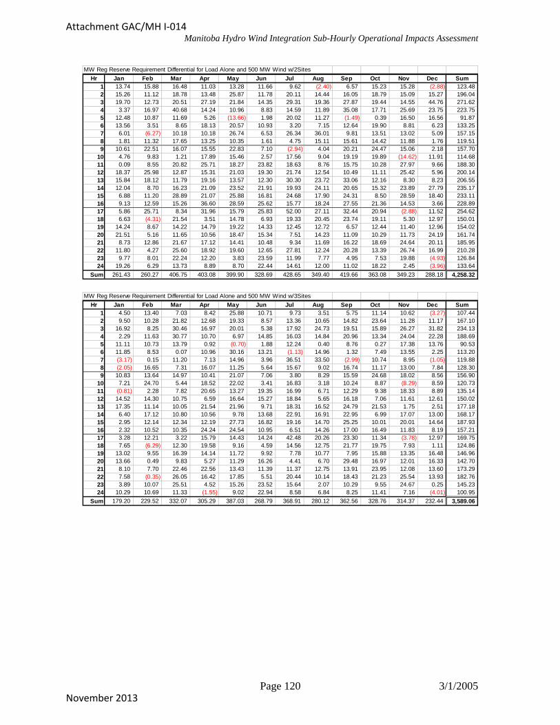
Manitoba Hydro Wind Integration Sub-Hourly Operational Impacts Assessment
MW Reg Reserve Requirement Differential for Load Alone and 500 MW Wind w/2Sites
Hr Jan Feb Mar Apr May Jun Jul Aug Sep Oct Nov Dec Sum1 13.74 15.88 16.48 11.03 13.28 11.66 9.62 (2.40) (2.88)
(13.66) (1.49)
(6.27)
(2.94)(14.62)
(2.88)(4.31)
(4.93)(3.96)
6.57 15.23 15.28 123.482 15.26 11.12 18.78 13.48 25.87 11.78 20.11 14.44 16.05 18.79 15.09 15.27 196.043 19.70 12.73 20.51 27.19 21.84 14.35 29.31 19.36 27.87 19.44 14.55 44.76 271.624 3.37 16.97 40.68 14.24 10.96 8.83 14.59 11.89 35.08 17.71 25.69 23.75 223.755 12.48 10.87 11.69 5.26 1.98 20.02 11.27 0.39 16.50 16.56 91.876 13.56 3.51 8.65 18.13 20.57 10.93 3.20 7.15 12.64 19.90 8.81 6.23 133.257 6.01 10.18 10.18 26.74 6.53 26.34 36.01 9.81 13.51 13.02 5.09 157.158 1.81 11.32 17.65 13.25 10.35 1.61 4.75 15.11 15.61 14.42 11.88 1.76 119.519 10.61 22.51 16.07 15.55 22.83 7.10 4.04 20.21 24.47 15.06 2.18 157.70
10 4.76 9.83 1.21 17.89 15.46 2.57 17.56 9.04 19.19 19.89 11.91 114.6811 0.09 8.55 20.82 25.71 18.27 23.82 18.63 8.76 15.75 10.28 27.97 9.66 188.3012 18.37 25.98 12.87 15.31 21.03 19.30 21.74 12.54 10.49 11.11 25.42 5.96 200.1413 15.84 18.12 11.79 19.16 13.57 12.30 30.30 23.72 33.06 12.16 8.30 8.23 206.5514 12.04 8.70 16.23 21.09 23.52 21.91 19.93 24.11 20.65 15.32 23.89 27.79 235.1715 6.88 11.20 28.89 21.07 25.88 16.81 24.68 17.90 24.31 8.50 28.59 18.40 233.1116 9.13 12.59 15.26 36.60 28.59 25.62 15.77 18.24 27.55 21.36 14.53 3.66 228.8917 5.86 25.71 8.34 31.96 15.79 25.83 52.00 27.11 32.44 20.94 11.52 254.6218 6.63 21.54 3.51 14.78 6.93 19.33 20.45 23.74 19.11 5.30 12.97 150.0119 14.24 8.67 14.22 14.79 19.22 14.33 12.45 12.72 6.57 12.44 11.40 12.96 154.0220 21.51 5.16 11.65 10.56 18.47 15.34 7.51 14.23 11.09 10.29 11.73 24.19 161.7421 8.73 12.86 21.67 17.12 14.41 10.48 9.34 11.69 16.22 18.69 24.64 20.11 185.9522 11.80 4.27 25.60 18.92 19.60 12.65 27.81 12.24 20.28 13.39 26.74 16.99 210.2823 9.77 8.01 22.24 12.20 3.83 23.59 11.99 7.77 4.95 7.53 19.88 126.8424 19.26 6.29 13.73 8.89 8.70 22.44 14.61 12.00 11.02 18.22 2.45 133.64
Sum 261.43 260.27 406.75 403.08 399.90 328.69 428.65 349.40 419.66 363.08 349.23 288.18 4,258.32
MW Reg Reserve Requirement Differential for Load Alone and 500 MW Wind w/3Sites
Hr Jan Feb Mar Apr May Jun Jul Aug Sep Oct Nov Dec Sum1 4.50 13.40 7.03 8.42 25.88 10.71 9.73 3.51 5.75 11.14 10.62 (3.27)
(0.70)(1.13)
(3.17) (2.99) (1.05)(2.05)
(8.29)(0.81)
(3.78)(6.29)
(0.35)
(1.55) (4.01)
107.442 9.50 10.28 21.82 12.68 19.33 8.57 13.36 10.65 14.82 23.64 11.28 11.17 167.103 16.92 8.25 30.46 16.97 20.01 5.38 17.92 24.73 19.51 15.89 26.27 31.82 234.134 2.29 11.63 30.77 10.70 6.97 14.85 16.03 14.84 20.96 13.34 24.04 22.28 188.695 11.11 10.73 13.79 0.92 1.88 12.24 0.40 8.76 0.27 17.38 13.76 90.536 11.85 8.53 0.07 10.96 30.16 13.21 14.96 1.32 7.49 13.55 2.25 113.207 0.15 11.20 7.13 14.96 3.96 36.51 33.50 10.74 8.95 119.888 16.65 7.31 16.07 11.25 5.64 15.67 9.02 16.74 11.17 13.00 7.84 128.309 10.83 13.64 14.97 10.41 21.07 7.06 3.80 8.29 15.59 24.68 18.02 8.56 156.90
10 7.21 24.70 5.44 18.52 22.02 3.41 16.83 3.18 10.24 8.87 8.59 120.7311 2.28 7.82 20.65 13.27 19.35 16.99 6.71 12.29 9.38 18.33 8.89 135.1412 14.52 14.30 10.75 6.59 16.64 15.27 18.84 5.65 16.18 7.06 11.61 12.61 150.0213 17.35 11.14 10.05 21.54 21.96 9.71 18.31 16.52 24.79 21.53 1.75 2.51 177.1814 6.40 17.12 10.80 10.56 9.78 13.68 22.91 16.91 22.95 6.99 17.07 13.00 168.1715 2.95 12.14 12.34 12.19 27.73 16.82 19.16 14.70 25.25 10.01 20.01 14.64 187.9316 2.32 10.52 10.35 24.24 24.54 10.95 6.51 14.26 17.00 16.49 11.83 8.19 157.2117 3.28 12.21 3.22 15.79 14.43 14.24 42.48 20.26 23.30 11.34 12.97 169.7518 7.65 12.30 19.58 9.16 4.59 14.56 12.75 21.77 19.75 7.93 1.11 124.8619 13.02 9.55 16.39 14.14 11.72 9.92 7.78 10.77 7.95 15.88 13.35 16.48 146.9620 13.66 0.49 9.83 5.27 11.29 16.26 4.41 6.70 29.48 16.97 12.01 16.33 142.7021 8.10 7.70 22.46 22.56 13.43 11.39 11.37 12.75 13.91 23.95 12.08 13.60 173.2922 7.58 26.05 16.42 17.85 5.51 20.44 10.14 18.43 21.23 25.54 13.93 182.7623 3.89 10.07 25.51 4.52 15.26 23.52 15.64 2.07 10.29 9.55 24.67 0.25 145.2324 10.29 10.69 11.33 9.02 22.94 8.58 6.84 8.25 11.41 7.16 100.95
Sum 179.20 229.52 332.07 305.29 387.03 268.79 368.91 280.12 362.56 328.76 314.37 232.44 3,589.06
Page 120 3/1/2005
Attachment GAC/MH I-014
November 2013
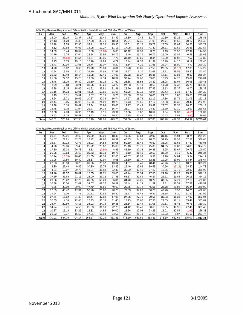
Manitoba Hydro Wind Integration Sub-Hourly Operational Impacts Assessment
MW Reg Reserve Requirement Differential for Load Alone and 600 MW Wind w/2Sites
Hr Jan Feb Mar Apr May Jun Jul Aug Sep Oct Nov Dec Sum1 16.00 22.10 22.37 14.67 21.40 13.42 14.30 0.45 11.77 20.39 20.26 1.67 178.812 22.13 14.20 25.35 17.28 33.71 18.61 25.21 17.46 21.09 23.71 19.50 20.17 258.433 25.78 18.55 27.90 32.11 28.32 15.35 37.01 25.15 35.78 25.55 22.03 54.25 347.794 4.12 22.58 46.98 18.08 19.27 11.15 17.98 16.85 41.49 24.51 33.65 26.88 283.545 14.89 15.44 18.67 6.80 (11.69)
(4.84)
(11.17)
(4.10)(3.92)
5.03 30.12 12.39 3.26 1.13 25.56 22.92 144.526 20.79 6.75 17.64 23.14 22.96 14.75 5.46 13.26 16.76 25.00 12.55 6.58 185.637 8.21 14.54 13.54 33.95 7.77 33.19 38.65 8.34 15.00 16.98 7.57 192.898 3.73 13.75 19.10 15.26 17.93 4.79 7.44 19.38 21.97 16.70 14.16 8.19 162.409 15.41 29.04 23.95 22.74 23.07 8.22 5.54 4.29 31.66 32.94 18.80 4.72 220.39
10 4.90 16.82 3.66 21.70 20.83 6.84 16.28 10.66 27.53 28.35 17.88 164.2911 0.64 13.58 22.20 32.19 22.68 27.48 25.57 9.10 22.68 12.81 38.56 15.30 242.8012 21.83 32.49 18.14 15.28 27.41 24.93 30.78 18.27 16.36 17.11 33.86 9.83 266.2713 21.66 24.37 15.25 19.60 17.14 18.34 37.44 29.67 39.80 16.93 14.76 15.89 270.8414 15.48 16.20 16.80 29.60 31.23 27.60 26.58 36.56 28.39 23.98 31.04 36.95 320.4115 9.79 18.68 38.21 30.26 33.21 24.22 27.88 23.11 30.59 11.28 32.42 25.70 305.3516 6.88 18.15 18.46 41.91 35.81 31.81 22.76 18.55 37.85 28.13 23.37 4.70 288.3817 10.16 34.32 12.01 42.95 19.55 31.67 61.28 30.12 42.94 30.43 1.38 17.49 334.2918 9.49 3.11 35.61 9.37 20.15 9.79 25.88 29.31 36.00 24.87 5.80 15.63 225.0119 18.54 13.71 19.69 20.27 30.33 16.74 19.27 18.78 12.12 17.86 13.76 21.05 222.1220 28.44 8.05 15.95 15.03 24.01 19.20 10.73 20.66 17.17 17.88 16.35 29.46 222.9221 13.38 15.18 29.41 22.34 21.96 15.66 13.77 15.44 23.82 27.57 33.37 28.25 260.1422 13.45 6.10 31.94 21.37 24.79 16.74 33.97 20.55 24.83 16.89 32.10 23.93 266.6623 10.68 7.78 26.95 17.19 9.11 29.94 13.56 8.82 10.52 9.34 22.30 162.0924 23.63 9.15 16.51 14.43 10.68 29.20 17.35 20.48 15.12 20.43 5.98 179.06
Sum 340.01 375.26 537.30 517.10 537.80 429.26 559.36 457.97 577.83 488.78 477.38 406.99 5,705.03 MW Reg Reserve Requirement Differential for Load Alone and 750 MW Wind w/2Sites
Hr Jan Feb Mar Apr May Jun Jul Aug Sep Oct Nov Dec Sum1 21.64 29.91 29.60 25.39 32.01 18.48 19.55 10.84 22.02 31.15 24.94 8.74 274.282 31.67 21.21 32.78 18.72 49.97 28.39 40.83 24.51 28.25 34.29 26.53 32.51 369.653 32.87 22.23 42.78 38.03 34.53 18.05 50.19 31.48 46.50 33.96 31.63 67.82 450.064 4.96 29.86 59.43 25.22 28.67 15.00 25.10 23.76 45.00 34.05 38.88 34.88 364.795 17.80 22.28 26.73 5.33 (7.80)
(10.79)
(0.19)
(1.63)
8.46 42.59 17.35 10.35 2.95 33.67 29.79 209.506 25.06 13.63 26.13 30.73 31.14 19.75 8.10 21.43 22.53 33.29 9.15 5.42 246.347 10.74 20.40 21.05 41.35 12.60 43.67 41.93 9.98 19.20 24.04 9.94 244.118 11.98 17.85 30.40 23.37 30.94 8.68 15.50 23.77 32.25 19.05 19.99 14.84 248.649 22.83 38.59 38.28 31.96 25.37 13.04 14.67 8.48 48.41 46.26 27.10 10.29 325.27
10 4.20 27.44 0.86 30.30 27.75 13.85 26.46 15.68 39.53 30.56 28.30 244.7311 4.21 19.07 30.78 41.04 31.80 32.48 35.50 12.40 37.22 19.35 52.75 22.32 338.9312 24.76 39.57 18.01 15.05 32.71 33.00 43.44 26.34 27.56 24.16 46.22 15.36 346.1713 37.59 35.58 21.16 24.00 26.32 27.31 54.87 37.86 46.27 25.51 21.53 26.18 384.1614 20.86 23.22 17.29 35.55 50.20 36.84 34.70 52.25 40.72 33.35 37.79 47.10 429.8615 16.88 35.00 52.67 33.07 42.27 36.57 35.44 34.19 41.59 18.81 36.52 37.58 420.5916 9.86 30.99 20.09 47.49 46.65 40.60 30.85 22.78 45.56 38.78 29.92 16.34 379.9017 12.85 43.42 17.34 57.26 26.92 40.76 77.03 39.20 56.76 43.26 3.53 14.26 432.6018 17.94 1.05 47.75 20.62 30.52 15.40 32.77 45.45 49.82 36.55 8.20 11.92 317.9919 27.61 16.52 21.49 32.47 47.59 17.95 27.56 27.70 29.56 30.33 16.33 27.82 322.9420 37.65 14.10 22.65 17.93 33.18 31.40 15.23 23.67 27.36 29.05 16.11 35.47 303.8121 24.74 29.69 43.13 28.92 24.76 19.38 22.54 19.44 31.06 39.51 45.46 40.76 369.3922 14.74 9.71 34.55 25.33 31.90 22.75 44.42 30.43 30.68 18.55 40.96 27.46 331.4823 10.27 15.18 33.25 22.32 14.85 36.00 16.26 12.03 23.25 12.01 32.54 226.3324 26.33 9.37 16.62 17.01 16.68 34.56 20.91 28.71 21.58 19.33 9.07 11.61 231.77
Sum 470.01 534.70 704.17 668.17 750.25 581.33 778.19 631.66 813.81 673.30 632.66 575.07 7,813.31
Page 121 3/1/2005
Attachment GAC/MH I-014
November 2013

Manitoba Hydro Wind Integration Sub-Hourly Operational Impacts Assessment
MW Reg Reserve Requirement Differential for Load Alone and 800 MW Wind w/2Sites
Hr Jan Feb Mar Apr May Jun Jul Aug Sep Oct Nov Dec Sum1 25.44 34.61 34.96 30.37 36.15 21.16 21.13 14.85 24.88 34.05 30.48 12.55 320.622 35.26 25.84 41.60 24.89 52.97 32.23 48.33 27.31 30.38 39.03 28.34 37.32 423.503 37.84 23.21 47.65 42.81 39.41 17.47 54.64 33.54 51.92 37.49 36.27 73.82 496.074 7.13 33.41 65.27 28.98 31.51 17.04 26.94 26.66 48.78 35.99 44.34 39.32 405.365 19.68 30.02 30.00 7.84 (8.99)
(3.70)
(2.48)
10.43 48.42 19.01 12.99 3.52 37.17 37.05 247.156 27.46 15.43 26.98 32.92 36.43 22.16 10.85 22.97 26.53 35.23 6.68 6.98 270.647 9.66 28.75 23.35 44.96 17.52 47.00 43.93 12.41 20.58 26.04 12.75 283.258 16.72 19.93 33.41 26.48 32.75 10.55 14.98 26.96 36.16 21.63 23.84 18.62 282.049 24.89 40.90 45.98 37.07 27.74 14.75 20.91 9.93 53.93 52.18 26.63 13.63 368.55
10 4.15 33.35 12.50 31.67 30.57 16.00 28.65 18.51 44.20 39.29 3.32 32.12 294.3311 7.21 22.67 33.33 44.36 36.55 34.85 42.07 15.15 41.96 23.67 57.58 25.75 385.1512 26.07 43.34 21.06 18.00 45.04 36.82 47.48 31.83 32.35 29.66 51.02 17.95 400.6113 42.04 38.87 23.16 29.94 27.56 35.58 61.38 41.78 51.03 27.36 25.45 30.29 434.4414 23.71 28.17 18.29 45.20 53.67 40.64 40.31 56.46 46.32 40.64 43.74 53.88 491.0315 20.49 37.16 56.78 43.41 45.89 38.76 42.62 37.96 46.70 22.40 43.16 40.50 475.8416 11.36 36.38 28.30 58.09 56.73 42.62 33.27 26.98 54.02 43.99 31.94 19.13 442.7917 15.87 50.22 21.31 64.82 33.64 42.42 81.82 43.00 61.12 53.20 5.77 23.02 496.2218 19.84 3.89 52.59 25.04 32.47 17.29 36.56 50.17 54.42 40.53 9.57 17.73 360.1219 30.01 22.85 22.11 36.70 52.65 18.58 28.93 30.88 36.02 35.43 20.15 33.66 367.9720 42.48 17.06 25.77 29.43 40.41 35.05 18.36 25.36 32.69 33.39 25.44 41.33 366.7521 29.54 37.97 45.69 33.97 34.13 24.91 23.50 24.21 41.71 45.66 44.16 45.82 431.2622 14.78 11.44 39.18 29.68 36.47 24.92 47.23 33.33 34.90 20.79 45.60 29.20 367.5223 11.29 16.22 32.44 25.16 24.64 38.23 16.14 13.90 27.17 14.81 35.53 253.0524 28.09 9.99 20.93 16.79 20.87 36.09 21.58 34.43 25.53 23.82 12.94 9.47 260.55
Sum 531.03 629.21 808.03 786.96 864.21 646.09 863.11 709.11 928.11 774.36 715.18 669.42 8,924.81
MW Reg Reserve Requirement Differential for Load Alone and 900 MW Wind w/2Sites
Hr Jan Feb Mar Apr May Jun Jul Aug Sep Oct Nov Dec Sum1 31.01 40.55 41.12 38.49 43.61 26.73 24.81 19.32 29.64 40.69 37.58 17.78 391.342 42.74 33.96 47.40 28.86 62.79 39.03 57.87 31.20 36.07 47.13 34.44 45.72 507.233 44.52 29.35 57.52 48.83 47.44 20.23 60.82 38.13 62.24 43.51 43.14 83.58 579.304 11.97 39.84 74.90 34.37 38.04 21.11 31.42 32.32 52.58 42.56 50.49 45.57 475.195 22.07 34.89 38.47 10.51 (6.42)
(3.40)
(1.07)
12.20 57.24 22.99 18.27 7.82 41.96 44.95 304.966 33.97 17.71 30.79 36.62 43.97 27.14 13.44 28.33 32.97 40.36 7.99 8.33 321.627 10.42 37.09 26.08 49.12 23.80 56.24 48.16 19.00 24.69 31.05 19.30 341.558 19.29 23.15 42.55 31.56 38.52 16.53 19.04 33.72 45.61 24.19 31.45 25.06 350.669 27.63 46.84 59.48 44.21 32.16 19.12 26.16 15.08 61.88 62.10 32.18 17.83 444.67
10 7.12 41.79 18.35 37.06 37.00 17.99 33.71 25.15 52.52 43.49 12.08 39.34 365.6111 10.34 28.57 39.18 49.06 42.84 39.22 49.32 21.26 49.88 32.03 66.61 31.57 459.8712 30.37 49.50 23.52 23.63 53.96 41.83 55.35 40.26 41.33 33.87 60.81 22.42 476.8513 51.85 46.49 27.93 38.93 34.93 44.19 74.02 50.38 56.61 34.68 33.92 40.83 534.7614 29.59 32.60 24.89 55.19 59.14 47.14 49.10 68.91 55.94 43.99 53.23 61.75 581.4615 24.96 47.82 66.07 55.03 53.09 45.51 52.29 46.39 57.07 29.18 49.24 45.71 572.3516 16.23 45.29 34.47 67.62 71.11 49.02 42.19 34.29 63.27 51.91 36.23 21.00 532.6217 17.75 59.79 28.16 75.73 40.10 49.96 91.05 50.11 70.72 65.72 10.63 24.89 584.6118 23.51 6.48 60.40 32.44 43.51 21.90 42.26 59.38 63.15 49.05 11.82 26.05 439.9419 36.12 27.36 22.83 44.98 64.57 23.83 33.20 36.89 42.23 44.15 24.00 43.25 443.4120 49.01 19.28 31.31 37.07 47.34 44.04 22.14 26.59 43.20 41.16 30.60 48.37 440.1221 36.76 51.19 52.97 42.08 40.47 32.68 28.38 29.81 49.50 54.70 50.66 52.64 521.8422 15.34 15.79 42.07 34.34 41.86 29.01 53.37 41.96 42.79 25.40 57.41 30.98 430.3323 16.05 18.16 36.71 30.83 28.99 38.52 17.46 16.04 35.37 23.09 44.34 304.4824 30.31 11.01 22.61 19.00 26.05 39.32 23.44 38.43 33.97 30.12 16.39 14.21 304.87
Sum 638.94 764.01 960.80 942.50 1,034.19 770.05 1,014.31 855.11 1,115.78 935.61 868.26 810.08 10,709.63
Page 122 3/1/2005
Attachment GAC/MH I-014
November 2013
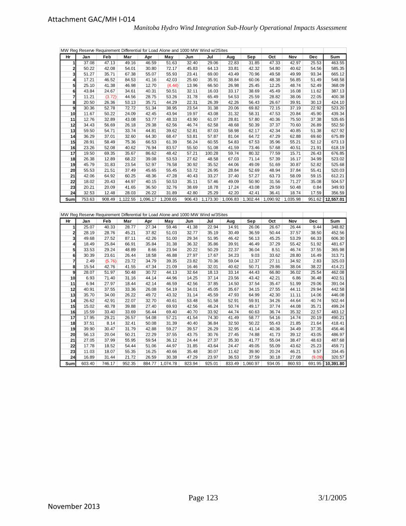
Manitoba Hydro Wind Integration Sub-Hourly Operational Impacts Assessment
MW Reg Reserve Requirement Differential for Load Alone and 1000 MW Wind w/2Sites
Hr Jan Feb Mar Apr May Jun Jul Aug Sep Oct Nov Dec Sum1 37.08 47.13 49.16 46.59 51.63 32.40 29.06 22.83 31.85 47.33 42.97 25.53 463.552 50.22 42.08 54.01 30.80 72.17 45.83 64.13 33.81 42.32 54.80 40.62 54.56 585.353 51.27 35.71 67.38 55.07 55.93 23.41 69.00 43.49 70.96 49.58 49.99 93.34 665.124 17.21 46.52 84.53 41.16 42.03 25.60 35.91 38.84 60.06 48.38 56.85 51.49 548.585 25.10 41.38 46.98 12.70 (4.44)
(3.72)
13.96 66.50 26.98 25.45 12.25 48.74 52.49 368.096 43.84 24.67 34.61 40.31 50.51 32.11 16.03 33.17 38.69 45.49 16.08 11.62 387.137 11.21 44.56 28.75 53.26 31.78 65.49 54.53 25.59 28.82 38.06 22.05 400.388 20.50 26.36 53.13 35.71 44.29 22.31 26.39 42.26 56.43 26.67 39.91 30.13 424.109 30.36 52.78 72.72 51.34 38.95 23.54 31.38 20.06 69.82 72.15 37.19 22.92 523.20
10 11.67 50.22 24.09 42.45 43.94 19.97 43.08 31.32 58.31 47.53 20.84 45.90 439.3411 12.76 32.89 43.08 53.77 48.33 43.90 61.07 28.81 57.80 40.36 75.50 37.38 535.6512 34.43 56.69 26.18 29.38 62.56 46.74 62.58 48.68 50.39 37.37 70.60 26.89 552.5013 59.50 54.71 33.74 44.81 39.62 52.81 87.03 58.98 62.17 42.34 40.85 51.38 627.9214 36.29 37.01 32.60 64.30 68.47 53.81 57.87 81.04 64.72 47.29 62.88 69.60 675.8915 28.91 58.49 75.36 66.53 61.39 56.24 60.55 54.83 67.53 35.96 55.21 52.12 673.1316 23.26 52.08 40.62 76.94 83.57 55.50 51.08 41.59 73.46 57.68 40.51 21.91 618.1917 19.50 69.35 35.67 86.62 48.42 57.21 100.28 59.74 80.32 77.59 15.71 26.43 676.8518 26.38 12.89 68.22 39.08 53.53 27.62 48.58 67.03 71.14 57.39 16.17 34.99 523.0219 45.79 31.83 23.54 52.97 76.58 30.92 35.52 44.06 49.09 51.69 30.87 52.82 525.6820 55.53 21.51 37.49 45.65 55.45 53.72 26.95 28.84 52.69 48.94 37.84 55.41 520.0321 42.06 64.92 60.25 48.36 47.28 40.43 33.27 37.40 57.27 63.73 58.09 59.15 612.2122 18.02 20.43 44.97 40.15 50.53 35.11 57.46 49.09 50.90 31.56 71.27 35.08 504.5723 20.21 20.09 41.65 36.50 32.76 38.69 18.78 17.24 43.08 29.59 50.48 0.84 349.9324 32.53 12.48 28.03 26.22 31.89 42.80 25.29 42.20 42.41 36.41 18.74 17.59 356.59
Sum 753.63 908.49 1,122.55 1,096.17 1,208.65 906.43 1,173.30 1,006.83 1,302.44 1,090.92 1,035.98 951.62 12,557.01 MW Reg Reserve Requirement Differential for Load Alone and 1000 MW Wind w/3Sites
Hr Jan Feb Mar Apr May Jun Jul Aug Sep Oct Nov Dec Sum1 25.07 40.33 28.77 27.34 59.46 41.38 22.94 14.91 26.06 26.67 26.44 9.44 348.822 28.19 28.76 45.21 37.82 51.03 32.77 35.19 30.49 36.59 50.44 37.57 38.50 452.563 49.68 27.52 87.11 42.26 51.00 29.34 51.95 46.42 56.13 45.25 53.29 66.33 606.304 18.49 25.84 66.91 35.84 31.38 36.32 35.86 39.91 46.49 37.29 55.42 51.92 481.675 33.53 29.24 48.89 8.66 23.94 20.22 50.29 22.37 36.04 8.51 46.74 37.55 365.986 30.39 23.61 26.44 18.58 46.88 27.97 17.67 34.23 9.03 33.62 28.80 16.49 313.717 2.49 (5.76)
(9.09)
23.72 34.79 39.35 23.82 70.36 59.04 12.37 27.11 34.92 2.83 325.038 15.54 42.76 41.55 47.34 21.09 16.46 32.01 40.62 50.71 29.86 38.04 38.22 414.219 28.07 51.97 50.48 30.72 44.13 32.64 18.13 33.14 44.43 66.80 36.02 25.54 462.08
10 6.93 71.40 31.16 44.14 44.96 14.25 37.14 23.56 43.42 42.21 6.86 36.48 402.5111 6.94 27.97 18.44 42.14 46.59 42.56 37.85 14.50 37.54 35.47 51.99 29.06 391.0412 40.91 37.55 33.36 26.08 54.19 34.01 45.05 35.67 34.15 27.55 44.11 29.94 442.5813 35.70 34.00 26.22 49.72 43.32 31.14 45.59 47.93 64.99 42.30 11.11 14.06 446.0814 26.62 42.91 22.07 32.70 40.61 53.48 51.58 52.91 59.91 34.26 44.64 40.74 502.4415 15.02 40.78 39.88 27.40 69.93 42.56 46.24 50.74 49.17 37.74 44.08 35.71 499.2416 15.59 33.40 33.69 56.44 69.40 40.70 33.92 44.74 60.63 36.74 35.32 22.57 483.1217 17.95 29.21 26.57 54.08 57.21 41.54 74.30 41.49 58.77 54.16 14.74 20.19 490.2118 37.51 8.14 32.41 50.08 31.39 40.40 36.84 32.50 50.22 55.43 21.85 21.64 418.4119 39.90 30.47 31.79 42.88 59.27 39.57 26.29 32.95 41.14 40.36 34.49 37.35 456.4620 56.13 20.04 50.21 22.29 37.55 43.75 30.76 27.45 74.88 41.73 39.12 43.05 486.9721 27.05 37.99 55.95 59.54 36.12 24.44 27.37 35.30 41.77 55.04 38.47 48.63 487.6822 17.78 18.52 54.44 51.06 44.97 31.85 43.64 24.47 49.05 55.09 43.62 25.23 459.7123 11.03 18.07 55.35 16.25 40.66 35.48 30.07 11.62 39.90 20.24 46.21 9.57 334.4524 16.89 31.44 21.72 26.59 30.38 47.29 23.97 36.53 37.59 30.18 27.08 320.57
Sum 603.40 746.17 952.35 884.77 1,074.78 823.94 925.01 833.49 1,060.97 934.05 860.93 691.95 10,391.80
Page 123 3/1/2005
Attachment GAC/MH I-014
November 2013
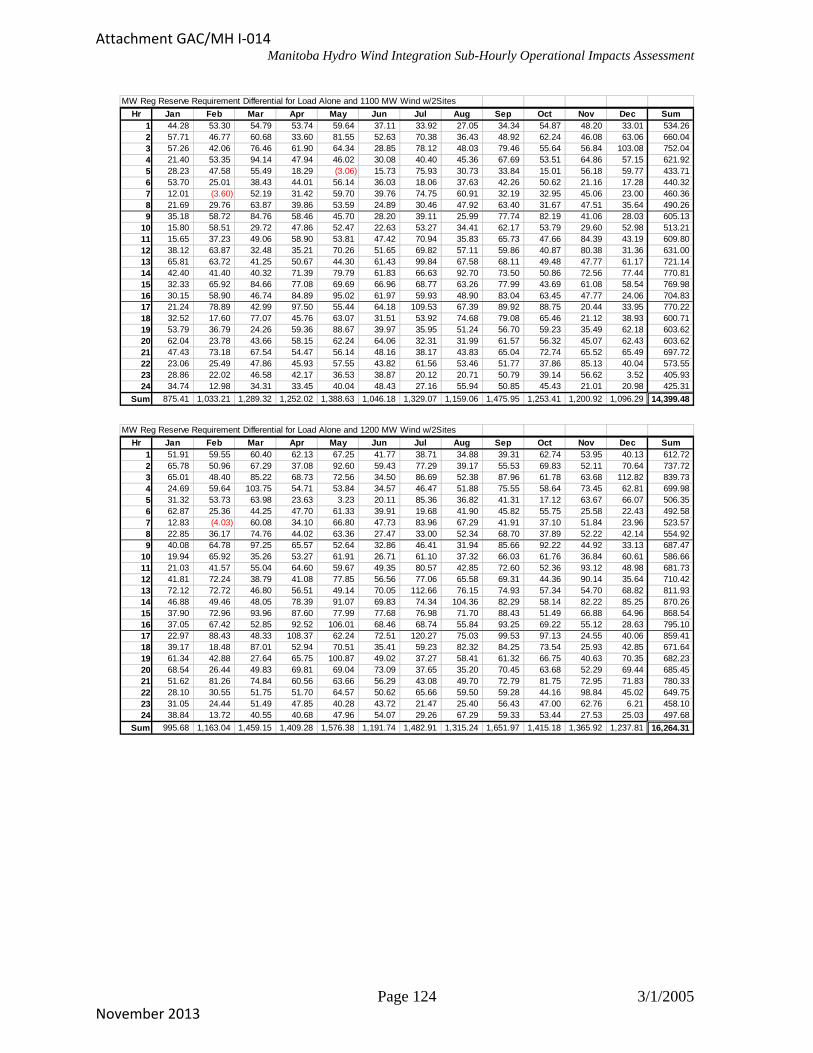
Manitoba Hydro Wind Integration Sub-Hourly Operational Impacts Assessment
MW Reg Reserve Requirement Differential for Load Alone and 1100 MW Wind w/2Sites
Hr Jan Feb Mar Apr May Jun Jul Aug Sep Oct Nov Dec Sum1 44.28 53.30 54.79 53.74 59.64 37.11 33.92 27.05 34.34 54.87 48.20 33.01 534.262 57.71 46.77 60.68 33.60 81.55 52.63 70.38 36.43 48.92 62.24 46.08 63.06 660.043 57.26 42.06 76.46 61.90 64.34 28.85 78.12 48.03 79.46 55.64 56.84 103.08 752.044 21.40 53.35 94.14 47.94 46.02 30.08 40.40 45.36 67.69 53.51 64.86 57.15 621.925 28.23 47.58 55.49 18.29 (3.06)
(3.60)
15.73 75.93 30.73 33.84 15.01 56.18 59.77 433.716 53.70 25.01 38.43 44.01 56.14 36.03 18.06 37.63 42.26 50.62 21.16 17.28 440.327 12.01 52.19 31.42 59.70 39.76 74.75 60.91 32.19 32.95 45.06 23.00 460.368 21.69 29.76 63.87 39.86 53.59 24.89 30.46 47.92 63.40 31.67 47.51 35.64 490.269 35.18 58.72 84.76 58.46 45.70 28.20 39.11 25.99 77.74 82.19 41.06 28.03 605.13
10 15.80 58.51 29.72 47.86 52.47 22.63 53.27 34.41 62.17 53.79 29.60 52.98 513.2111 15.65 37.23 49.06 58.90 53.81 47.42 70.94 35.83 65.73 47.66 84.39 43.19 609.8012 38.12 63.87 32.48 35.21 70.26 51.65 69.82 57.11 59.86 40.87 80.38 31.36 631.0013 65.81 63.72 41.25 50.67 44.30 61.43 99.84 67.58 68.11 49.48 47.77 61.17 721.1414 42.40 41.40 40.32 71.39 79.79 61.83 66.63 92.70 73.50 50.86 72.56 77.44 770.8115 32.33 65.92 84.66 77.08 69.69 66.96 68.77 63.26 77.99 43.69 61.08 58.54 769.9816 30.15 58.90 46.74 84.89 95.02 61.97 59.93 48.90 83.04 63.45 47.77 24.06 704.8317 21.24 78.89 42.99 97.50 55.44 64.18 109.53 67.39 89.92 88.75 20.44 33.95 770.2218 32.52 17.60 77.07 45.76 63.07 31.51 53.92 74.68 79.08 65.46 21.12 38.93 600.7119 53.79 36.79 24.26 59.36 88.67 39.97 35.95 51.24 56.70 59.23 35.49 62.18 603.6220 62.04 23.78 43.66 58.15 62.24 64.06 32.31 31.99 61.57 56.32 45.07 62.43 603.6221 47.43 73.18 67.54 54.47 56.14 48.16 38.17 43.83 65.04 72.74 65.52 65.49 697.7222 23.06 25.49 47.86 45.93 57.55 43.82 61.56 53.46 51.77 37.86 85.13 40.04 573.5523 28.86 22.02 46.58 42.17 36.53 38.87 20.12 20.71 50.79 39.14 56.62 3.52 405.9324 34.74 12.98 34.31 33.45 40.04 48.43 27.16 55.94 50.85 45.43 21.01 20.98 425.31
Sum 875.41 1,033.21 1,289.32 1,252.02 1,388.63 1,046.18 1,329.07 1,159.06 1,475.95 1,253.41 1,200.92 1,096.29 14,399.48 MW Reg Reserve Requirement Differential for Load Alone and 1200 MW Wind w/2Sites
Hr Jan Feb Mar Apr May Jun Jul Aug Sep Oct Nov Dec Sum1 51.91 59.55 60.40 62.13 67.25 41.77 38.71 34.88 39.31 62.74 53.95 40.13 612.722 65.78 50.96 67.29 37.08 92.60 59.43 77.29 39.17 55.53 69.83 52.11 70.64 737.723 65.01 48.40 85.22 68.73 72.56 34.50 86.69 52.38 87.96 61.78 63.68 112.82 839.734 24.69 59.64 103.75 54.71 53.84 34.57 46.47 51.88 75.55 58.64 73.45 62.81 699.985 31.32 53.73 63.98 23.63 3.23 20.11 85.36 36.82 41.31 17.12 63.67 66.07 506.356 62.87 25.36 44.25 47.70 61.33 39.91 19.68 41.90 45.82 55.75 25.58 22.43 492.587 12.83 (4.03) 60.08 34.10 66.80 47.73 83.96 67.29 41.91 37.10 51.84 23.96 523.578 22.85 36.17 74.76 44.02 63.36 27.47 33.00 52.34 68.70 37.89 52.22 42.14 554.929 40.08 64.78 97.25 65.57 52.64 32.86 46.41 31.94 85.66 92.22 44.92 33.13 687.47
10 19.94 65.92 35.26 53.27 61.91 26.71 61.10 37.32 66.03 61.76 36.84 60.61 586.6611 21.03 41.57 55.04 64.60 59.67 49.35 80.57 42.85 72.60 52.36 93.12 48.98 681.7312 41.81 72.24 38.79 41.08 77.85 56.56 77.06 65.58 69.31 44.36 90.14 35.64 710.4213 72.12 72.72 46.80 56.51 49.14 70.05 112.66 76.15 74.93 57.34 54.70 68.82 811.9314 46.88 49.46 48.05 78.39 91.07 69.83 74.34 104.36 82.29 58.14 82.22 85.25 870.2615 37.90 72.96 93.96 87.60 77.99 77.68 76.98 71.70 88.43 51.49 66.88 64.96 868.5416 37.05 67.42 52.85 92.52 106.01 68.46 68.74 55.84 93.25 69.22 55.12 28.63 795.1017 22.97 88.43 48.33 108.37 62.24 72.51 120.27 75.03 99.53 97.13 24.55 40.06 859.4118 39.17 18.48 87.01 52.94 70.51 35.41 59.23 82.32 84.25 73.54 25.93 42.85 671.6419 61.34 42.88 27.64 65.75 100.87 49.02 37.27 58.41 61.32 66.75 40.63 70.35 682.2320 68.54 26.44 49.83 69.81 69.04 73.09 37.65 35.20 70.45 63.68 52.29 69.44 685.4521 51.62 81.26 74.84 60.56 63.66 56.29 43.08 49.70 72.79 81.75 72.95 71.83 780.3322 28.10 30.55 51.75 51.70 64.57 50.62 65.66 59.50 59.28 44.16 98.84 45.02 649.7523 31.05 24.44 51.49 47.85 40.28 43.72 21.47 25.40 56.43 47.00 62.76 6.21 458.1024 38.84 13.72 40.55 40.68 47.96 54.07 29.26 67.29 59.33 53.44 27.53 25.03 497.68
Sum 995.68 1,163.04 1,459.15 1,409.28 1,576.38 1,191.74 1,482.91 1,315.24 1,651.97 1,415.18 1,365.92 1,237.81 16,264.31
Page 124 3/1/2005
Attachment GAC/MH I-014
November 2013
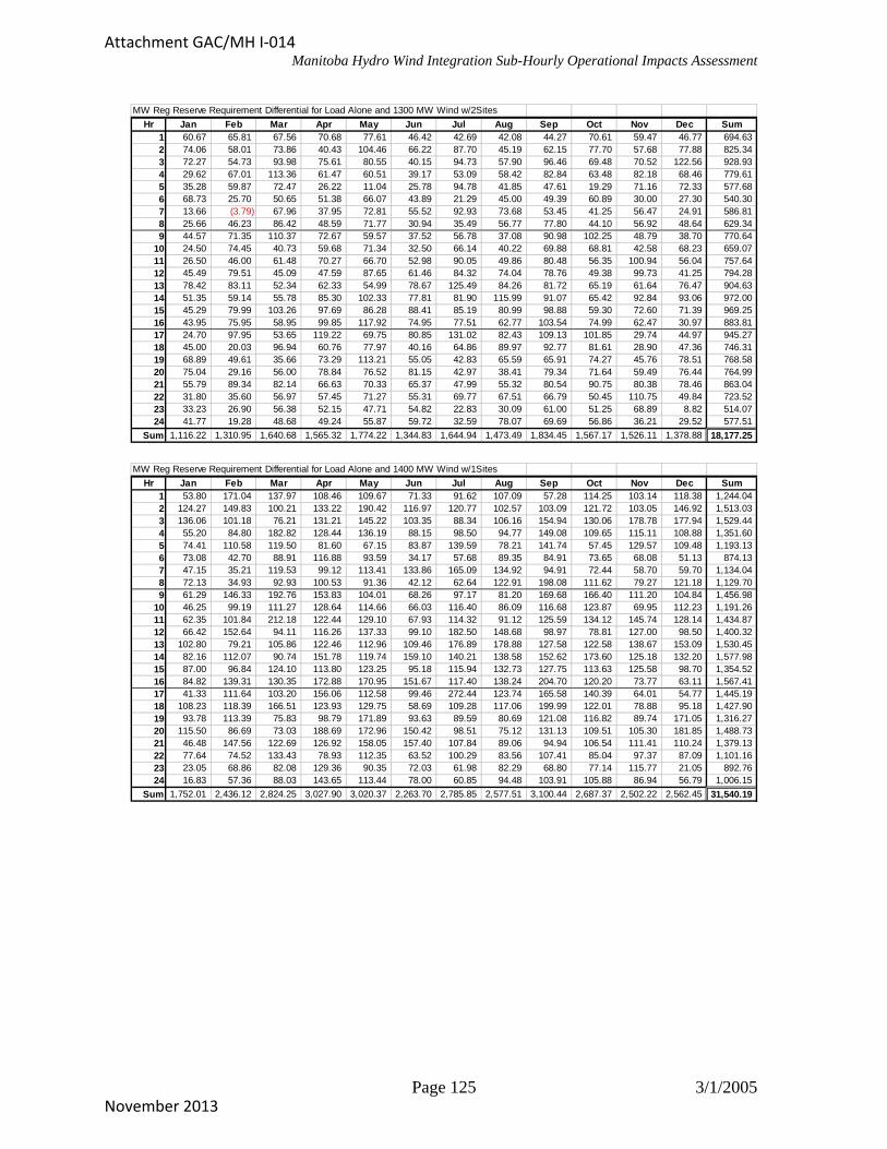
Manitoba Hydro Wind Integration Sub-Hourly Operational Impacts Assessment
MW Reg Reserve Requirement Differential for Load Alone and 1300 MW Wind w/2Sites
Hr Jan Feb Mar Apr May Jun Jul Aug Sep Oct Nov Dec Sum1 60.67 65.81 67.56 70.68 77.61 46.42 42.69 42.08 44.27 70.61 59.47 46.77 694.632 74.06 58.01 73.86 40.43 104.46 66.22 87.70 45.19 62.15 77.70 57.68 77.88 825.343 72.27 54.73 93.98 75.61 80.55 40.15 94.73 57.90 96.46 69.48 70.52 122.56 928.934 29.62 67.01 113.36 61.47 60.51 39.17 53.09 58.42 82.84 63.48 82.18 68.46 779.615 35.28 59.87 72.47 26.22 11.04 25.78 94.78 41.85 47.61 19.29 71.16 72.33 577.686 68.73 25.70 50.65 51.38 66.07 43.89 21.29 45.00 49.39 60.89 30.00 27.30 540.307 13.66 (3.79) 67.96 37.95 72.81 55.52 92.93 73.68 53.45 41.25 56.47 24.91 586.818 25.66 46.23 86.42 48.59 71.77 30.94 35.49 56.77 77.80 44.10 56.92 48.64 629.349 44.57 71.35 110.37 72.67 59.57 37.52 56.78 37.08 90.98 102.25 48.79 38.70 770.64
10 24.50 74.45 40.73 59.68 71.34 32.50 66.14 40.22 69.88 68.81 42.58 68.23 659.0711 26.50 46.00 61.48 70.27 66.70 52.98 90.05 49.86 80.48 56.35 100.94 56.04 757.6412 45.49 79.51 45.09 47.59 87.65 61.46 84.32 74.04 78.76 49.38 99.73 41.25 794.2813 78.42 83.11 52.34 62.33 54.99 78.67 125.49 84.26 81.72 65.19 61.64 76.47 904.6314 51.35 59.14 55.78 85.30 102.33 77.81 81.90 115.99 91.07 65.42 92.84 93.06 972.0015 45.29 79.99 103.26 97.69 86.28 88.41 85.19 80.99 98.88 59.30 72.60 71.39 969.2516 43.95 75.95 58.95 99.85 117.92 74.95 77.51 62.77 103.54 74.99 62.47 30.97 883.8117 24.70 97.95 53.65 119.22 69.75 80.85 131.02 82.43 109.13 101.85 29.74 44.97 945.2718 45.00 20.03 96.94 60.76 77.97 40.16 64.86 89.97 92.77 81.61 28.90 47.36 746.3119 68.89 49.61 35.66 73.29 113.21 55.05 42.83 65.59 65.91 74.27 45.76 78.51 768.5820 75.04 29.16 56.00 78.84 76.52 81.15 42.97 38.41 79.34 71.64 59.49 76.44 764.9921 55.79 89.34 82.14 66.63 70.33 65.37 47.99 55.32 80.54 90.75 80.38 78.46 863.0422 31.80 35.60 56.97 57.45 71.27 55.31 69.77 67.51 66.79 50.45 110.75 49.84 723.5223 33.23 26.90 56.38 52.15 47.71 54.82 22.83 30.09 61.00 51.25 68.89 8.82 514.0724 41.77 19.28 48.68 49.24 55.87 59.72 32.59 78.07 69.69 56.86 36.21 29.52 577.51
Sum 1,116.22 1,310.95 1,640.68 1,565.32 1,774.22 1,344.83 1,644.94 1,473.49 1,834.45 1,567.17 1,526.11 1,378.88 18,177.25
MW Reg Reserve Requirement Differential for Load Alone and 1400 MW Wind w/1Sites
Hr Jan Feb Mar Apr May Jun Jul Aug Sep Oct Nov Dec Sum1 53.80 171.04 137.97 108.46 109.67 71.33 91.62 107.09 57.28 114.25 103.14 118.38 1,244.042 124.27 149.83 100.21 133.22 190.42 116.97 120.77 102.57 103.09 121.72 103.05 146.92 1,513.033 136.06 101.18 76.21 131.21 145.22 103.35 88.34 106.16 154.94 130.06 178.78 177.94 1,529.444 55.20 84.80 182.82 128.44 136.19 88.15 98.50 94.77 149.08 109.65 115.11 108.88 1,351.605 74.41 110.58 119.50 81.60 67.15 83.87 139.59 78.21 141.74 57.45 129.57 109.48 1,193.136 73.08 42.70 88.91 116.88 93.59 34.17 57.68 89.35 84.91 73.65 68.08 51.13 874.137 47.15 35.21 119.53 99.12 113.41 133.86 165.09 134.92 94.91 72.44 58.70 59.70 1,134.048 72.13 34.93 92.93 100.53 91.36 42.12 62.64 122.91 198.08 111.62 79.27 121.18 1,129.709 61.29 146.33 192.76 153.83 104.01 68.26 97.17 81.20 169.68 166.40 111.20 104.84 1,456.98
10 46.25 99.19 111.27 128.64 114.66 66.03 116.40 86.09 116.68 123.87 69.95 112.23 1,191.2611 62.35 101.84 212.18 122.44 129.10 67.93 114.32 91.12 125.59 134.12 145.74 128.14 1,434.8712 66.42 152.64 94.11 116.26 137.33 99.10 182.50 148.68 98.97 78.81 127.00 98.50 1,400.3213 102.80 79.21 105.86 122.46 112.96 109.46 176.89 178.88 127.58 122.58 138.67 153.09 1,530.4514 82.16 112.07 90.74 151.78 119.74 159.10 140.21 138.58 152.62 173.60 125.18 132.20 1,577.9815 87.00 96.84 124.10 113.80 123.25 95.18 115.94 132.73 127.75 113.63 125.58 98.70 1,354.5216 84.82 139.31 130.35 172.88 170.95 151.67 117.40 138.24 204.70 120.20 73.77 63.11 1,567.4117 41.33 111.64 103.20 156.06 112.58 99.46 272.44 123.74 165.58 140.39 64.01 54.77 1,445.1918 108.23 118.39 166.51 123.93 129.75 58.69 109.28 117.06 199.99 122.01 78.88 95.18 1,427.9019 93.78 113.39 75.83 98.79 171.89 93.63 89.59 80.69 121.08 116.82 89.74 171.05 1,316.2720 115.50 86.69 73.03 188.69 172.96 150.42 98.51 75.12 131.13 109.51 105.30 181.85 1,488.7321 46.48 147.56 122.69 126.92 158.05 157.40 107.84 89.06 94.94 106.54 111.41 110.24 1,379.1322 77.64 74.52 133.43 78.93 112.35 63.52 100.29 83.56 107.41 85.04 97.37 87.09 1,101.1623 23.05 68.86 82.08 129.36 90.35 72.03 61.98 82.29 68.80 77.14 115.77 21.05 892.7624 16.83 57.36 88.03 143.65 113.44 78.00 60.85 94.48 103.91 105.88 86.94 56.79 1,006.15
Sum 1,752.01 2,436.12 2,824.25 3,027.90 3,020.37 2,263.70 2,785.85 2,577.51 3,100.44 2,687.37 2,502.22 2,562.45 31,540.19
Page 125 3/1/2005
Attachment GAC/MH I-014
November 2013

Manitoba Hydro Wind Integration Sub-Hourly Operational Impacts Assessment
MW Reg Reserve Requirement Differential for Load Alone and 1400 MW Wind w/2Sites
Hr Jan Feb Mar Apr May Jun Jul Aug Sep Oct Nov Dec Sum1 70.94 72.30 76.13 78.83 87.96 51.13 43.36 46.50 49.22 78.47 64.67 53.41 772.922 82.34 65.81 79.15 45.03 116.32 73.01 97.68 51.22 68.77 85.57 62.62 84.98 912.493 79.30 61.06 102.74 82.92 89.61 45.92 102.79 64.24 104.99 77.26 77.35 132.29 1,020.474 32.89 74.25 122.96 68.23 67.19 44.25 59.77 65.01 91.25 67.95 90.91 74.67 859.315 38.42 65.99 80.96 28.43 17.02 31.45 104.19 45.84 53.91 21.47 78.39 78.55 644.616 74.58 30.28 57.05 55.07 70.81 47.87 25.85 47.48 52.96 66.03 34.42 30.63 593.037 14.93 3.39 75.83 42.96 77.44 59.38 101.91 80.25 64.16 45.41 61.10 25.86 652.618 29.89 56.28 102.84 54.82 79.78 34.87 37.21 61.19 87.43 50.31 61.64 55.15 711.429 48.23 77.92 123.50 80.07 66.48 42.18 66.72 41.87 97.57 112.27 52.65 45.71 855.19
10 29.82 81.69 46.12 66.74 80.53 38.86 70.13 43.13 73.73 75.55 49.15 75.84 731.2811 31.73 50.93 68.43 75.94 73.72 56.61 98.52 58.42 88.81 63.73 108.77 63.09 838.6912 49.18 85.87 51.40 55.58 97.59 66.36 92.61 82.49 88.21 55.69 108.78 46.90 880.6613 86.95 96.91 57.88 68.14 61.76 85.64 138.31 92.36 88.50 71.76 68.59 84.11 1,000.9014 55.83 68.81 63.52 92.15 113.57 85.78 89.45 126.91 99.86 72.96 102.34 100.85 1,072.0415 52.05 87.03 112.56 106.45 94.58 98.79 93.38 90.62 109.32 66.89 78.26 77.81 1,067.7316 50.85 84.79 65.03 107.07 129.60 81.44 86.24 69.70 114.28 80.77 69.82 33.31 972.9017 29.07 107.47 58.97 130.07 77.65 89.19 141.78 89.74 118.74 105.75 37.37 49.88 1,035.6918 50.50 22.88 106.24 68.57 85.42 47.18 70.48 97.78 101.28 89.68 32.63 55.94 828.5819 76.43 57.10 44.90 81.29 125.54 62.82 48.40 72.77 70.47 82.77 50.87 86.66 860.0320 81.53 32.28 62.16 87.88 85.40 89.19 48.28 41.61 88.53 79.86 66.79 84.03 847.5421 59.96 97.43 89.45 73.66 76.96 74.44 52.91 60.64 87.52 99.75 87.80 85.86 946.3622 35.28 40.88 62.30 63.19 81.57 57.56 73.88 74.22 74.29 57.25 119.45 54.33 794.2023 35.41 29.35 61.26 55.83 58.15 62.77 25.94 34.79 65.57 55.43 75.42 11.32 571.2524 45.22 21.20 57.24 57.98 65.12 65.39 36.24 85.51 80.06 65.81 39.07 34.02 652.86
Sum 1,241.31 1,471.89 1,828.61 1,726.88 1,979.78 1,492.10 1,806.06 1,624.28 2,019.44 1,728.37 1,678.83 1,525.20 20,122.73 MW Reg Reserve Requirement Differential for Load Alone and 1400 MW Wind w/3Sites
Hr Jan Feb Mar Apr May Jun Jul Aug Sep Oct Nov Dec Sum1 48.60 62.29 45.28 60.90 94.43 58.86 44.71 36.30 44.41 43.76 47.23 32.83 619.602 51.51 47.01 63.44 53.92 78.23 49.57 55.29 53.14 65.11 75.84 57.94 62.35 713.353 71.26 46.98 132.62 65.42 74.31 45.39 94.78 62.46 89.52 70.61 77.50 100.32 931.184 33.91 43.47 100.43 53.88 56.87 53.82 63.90 66.45 73.60 64.18 88.86 70.67 770.075 41.26 48.85 88.58 22.63 38.77 41.46 72.10 33.96 60.61 20.84 76.94 63.29 609.286 45.94 26.66 41.19 24.12 58.21 43.48 30.07 53.31 17.89 47.40 49.79 33.66 471.727 8.10 1.35 47.09 61.33 62.25 47.76 89.18 77.66 24.34 47.20 51.74 13.46 531.478 30.10 65.20 71.99 75.63 48.78 30.49 48.25 68.68 68.26 41.52 55.13 63.53 667.579 40.70 87.43 86.03 50.19 67.82 52.91 43.34 56.00 69.39 101.33 50.06 55.69 760.90
10 16.91 105.04 52.90 62.76 80.98 25.81 75.33 38.39 59.75 68.35 29.94 64.05 680.2111 23.47 55.88 36.92 70.59 78.37 54.17 62.81 28.64 55.92 61.78 80.07 54.86 663.4812 58.31 59.81 59.50 43.64 88.84 49.25 70.26 65.18 64.06 40.70 67.81 50.60 717.9613 54.26 49.71 40.91 82.83 62.83 61.20 67.45 76.14 98.46 58.80 26.85 33.31 712.7314 45.73 64.58 34.45 59.12 77.70 83.79 76.70 89.24 95.60 62.89 63.67 63.86 817.3415 27.59 68.05 64.71 54.39 103.11 55.77 73.53 81.17 78.43 59.06 61.85 51.82 779.4916 22.96 54.09 55.89 81.82 107.57 62.22 53.28 70.73 96.78 66.20 53.34 43.92 768.8117 32.44 45.83 50.24 86.40 92.45 71.47 104.81 63.85 81.02 86.44 25.41 23.81 764.1718 50.80 31.34 55.61 83.32 64.21 68.37 60.87 58.74 79.83 85.02 35.26 35.44 708.8119 66.38 50.43 51.67 68.97 103.44 65.43 48.80 53.47 72.91 59.93 52.03 49.20 742.6620 82.10 40.27 75.10 55.58 64.40 58.47 52.15 36.60 115.22 60.96 60.83 61.41 763.0921 42.50 64.98 83.11 93.94 57.43 37.19 44.00 64.18 64.79 91.26 64.89 83.33 791.6122 30.09 35.09 83.15 74.57 74.74 58.01 67.89 42.26 84.01 86.16 57.45 45.85 739.2823 23.38 37.30 79.96 21.52 80.05 36.01 40.04 21.40 62.02 32.34 63.77 27.26 525.0424 33.73 75.92 35.78 57.21 49.38 73.22 45.28 60.99 60.49 44.88 44.51 2.83 584.22
Sum 982.07 1,267.58 1,536.56 1,464.70 1,765.16 1,284.11 1,484.82 1,358.92 1,682.43 1,477.47 1,342.88 1,187.34 16,834.05
Page 126 3/1/2005
Attachment GAC/MH I-014
November 2013
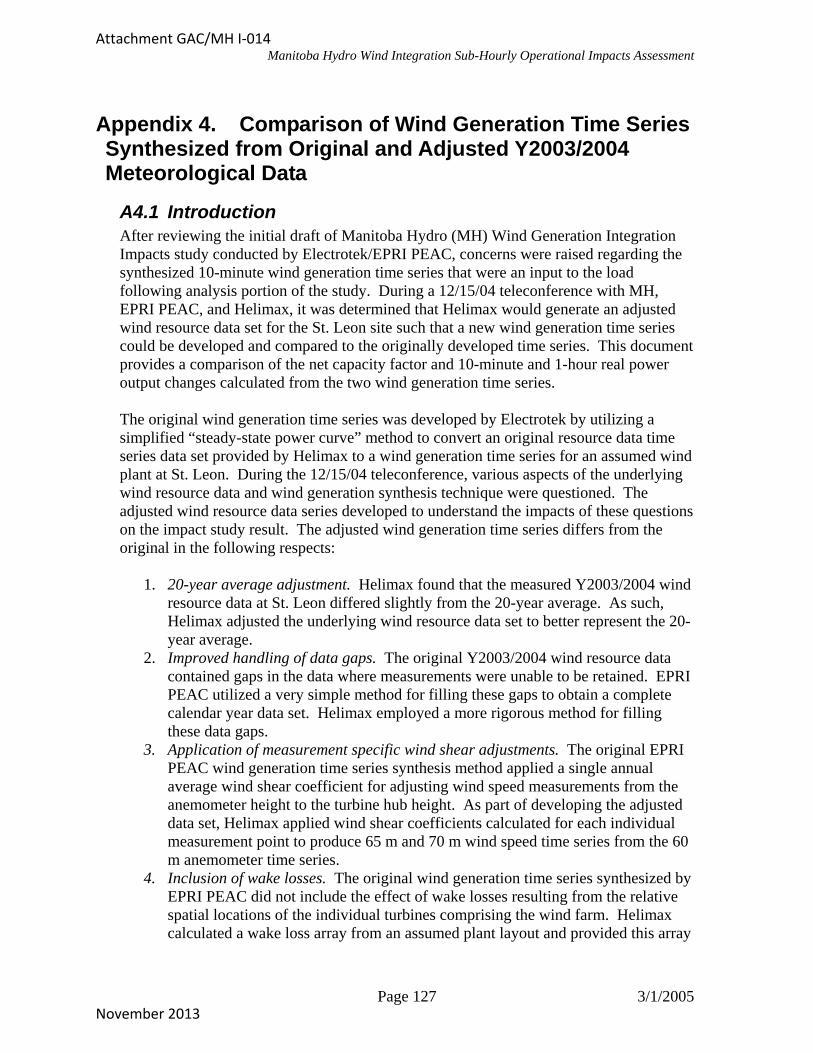
Manitoba Hydro Wind Integration Sub-Hourly Operational Impacts Assessment
Appendix 4. Comparison of Wind Generation Time Series Synthesized from Original and Adjusted Y2003/2004 Meteorological Data
A4.1 Introduction After reviewing the initial draft of Manitoba Hydro (MH) Wind Generation Integration Impacts study conducted by Electrotek/EPRI PEAC, concerns were raised regarding the synthesized 10-minute wind generation time series that were an input to the load following analysis portion of the study. During a 12/15/04 teleconference with MH, EPRI PEAC, and Helimax, it was determined that Helimax would generate an adjusted wind resource data set for the St. Leon site such that a new wind generation time series could be developed and compared to the originally developed time series. This document provides a comparison of the net capacity factor and 10-minute and 1-hour real power output changes calculated from the two wind generation time series. The original wind generation time series was developed by Electrotek by utilizing a simplified “steady-state power curve” method to convert an original resource data time series data set provided by Helimax to a wind generation time series for an assumed wind plant at St. Leon. During the 12/15/04 teleconference, various aspects of the underlying wind resource data and wind generation synthesis technique were questioned. The adjusted wind resource data series developed to understand the impacts of these questions on the impact study result. The adjusted wind generation time series differs from the original in the following respects:
1. 20-year average adjustment. Helimax found that the measured Y2003/2004 wind resource data at St. Leon differed slightly from the 20-year average. As such, Helimax adjusted the underlying wind resource data set to better represent the 20-year average.
2. Improved handling of data gaps. The original Y2003/2004 wind resource data contained gaps in the data where measurements were unable to be retained. EPRI PEAC utilized a very simple method for filling these gaps to obtain a complete calendar year data set. Helimax employed a more rigorous method for filling these data gaps.
3. Application of measurement specific wind shear adjustments. The original EPRI PEAC wind generation time series synthesis method applied a single annual average wind shear coefficient for adjusting wind speed measurements from the anemometer height to the turbine hub height. As part of developing the adjusted data set, Helimax applied wind shear coefficients calculated for each individual measurement point to produce 65 m and 70 m wind speed time series from the 60 m anemometer time series.
4. Inclusion of wake losses. The original wind generation time series synthesized by EPRI PEAC did not include the effect of wake losses resulting from the relative spatial locations of the individual turbines comprising the wind farm. Helimax calculated a wake loss array from an assumed plant layout and provided this array
Page 127 3/1/2005
Attachment GAC/MH I-014
November 2013

Manitoba Hydro Wind Integration Sub-Hourly Operational Impacts Assessment
to EPRI PEAC to be included in the adjusted wind generation time series synthesis.
A4.2 Synthesis of Adjusted Wind Generation Time Series Helimax provided the adjusted wind resource data set that incorporated the 20-year average adjustment, improved filling of data gaps, and application of per measurement point shear coefficients. EPRI PEAC altered the MS Access Visual Basic code utilized for synthesizing the wind generation time series to accommodate the per measurement wind shear adjustments and the inclusion of wake losses. The altered synthesis method was then applied to the adjusted wind resource data set. Note that two data gaps were found in the adjusted wind resource data set. These gaps were filled by copying data from the same clock period for the previous day as follows:
Data Gap Fill Data 12/29/2003 00:00 - 12/29/2003 11:50 12/28/2003 00:00 - 12/28/2003 11:50 1/14/2004 00:00 - 1/14/2004 17:50 1/13/2004 00:00 - 1/13/2004 17:50
The discontinuities created at the boundaries of these data gaps by inserting the fill data were found to be inconsequential.
A4.3 Comparison of Original and Adjusted Wind Generation Time Series
A4.3.1. Net Capacity Factor As part of a study conducted by Helimax related to the wind resource quality at the St. Leon, Helimax calculated a site net capacity factor of 38.86%. EPRI PEAC calculated a site net capacity factor of 42.32% from the original wind generation time series synthesized as indicated in the introduction section. It should be noted that the objectives of the Helimax study and the associated Helimax wind model was quite different from that of Electrotek/EPRI PEAC study and its associated wind model. Whereas the Helimax study was likely more related to wind resource assessment for estimating energy yield for planning purposes, the wind integration impact model was intended to provide a representation of the range and frequency of fluctuations in real power output on differing time resolutions for determining impact on operations, and not necessarily to accurately estimate the site capacity factors. Nonetheless, because Manitoba Hydro will likely be forced to address critics that might refer to the difference in capacity factors, it is important to explain the differences in the calculated values.
In an attempt to explain the differences in the originally calculated net capacity factor values, a revised net capacity factor was calculated from the adjusted wind generation time series. The adjusted wind generation time series yields a net capacity factor of 40.03%. The reduction in net capacity factor from 42.32% to 40.03% results from the combination of changes stated previously that yield the adjusted wind generation time series as compared to the original time series. Although one can’t isolate the impacts of each of the changes based on the aggregate comparison summarized here, it is likely that the primary reduction results from the inclusion of wake losses in the wind generation
Page 128 3/1/2005
Attachment GAC/MH I-014
November 2013

Manitoba Hydro Wind Integration Sub-Hourly Operational Impacts Assessment
synthesis method. It should also be noted that although the net impact of the adjustments is a reduction in capacity factor, specific changes such as the 20-year average adjustment might actually increase the capacity factor as Helimax had indicated that the original measurement data set was slightly below average.
As for explaining the remaining difference, a better understanding of Helimax’s exact approach is needed (i.e., what power curve used, handling of cold weather cut-out, how "other loss" factors are applied, etc.). Once all differences in calculation method are understood, these can be documented these in the final report to mitigate criticisms that might be aimed at the differences in capacity factor values calculated in the two studies.
A4.3.2. 10-Minute and 1-Hour Real Power Output Fluctuations The other concern to be addressed is to ensure that the full range and frequency of real power fluctuations (10-min and 1-hour time frames) are represented in the original data set. In order to gain a sense of how the revised wind speed data set (20-yr avg adjustment, improved data gap filling, individual data point wind shear adjustment, wake loss treatment) impacts the degree of real power fluctuations relative to those inherent in the original wind generation time series, the following are provided:
• Comparison of actual 10-minute resolution wind generation real power outputtime series for selected periods. Gives a visual sense of how adjustments affectthe wind plant fluctuations.
• Comparison of the 10-min and 1-hr real power output change probabilitydistributions. Gives a sense of how the wind speed adjustments might impact theload following reserve requirement calculations, but will only give us anapproximate representation as the LFRR calculation is obviously more involvedand based on the synthesized 1-min resolution data.
The wind generation time series and generation output change probability distributions are constructed from the following data sets:
• Original 10-minute resolution Y2003/2004 St. Leon wind generation output timeseries synthesized according to the method described in the Introduction sectionof this memo and in detail in Section 3.1 of the draft impact study report.
• Adjusted 10-minute resolution Y2003/2004 MH St. Leon wind generation realpower output time series synthesized according to the changes in the originalmethod described in the Introduction section of this memo.
The hourly change distributions are obtained directly from the 10-minute data series by aggregation of the 10-minute data to hourly average data. The “10-minute change” and “1-hour change” distributions are determined as the difference of one 10-minute average (or 1-hr average) value and the previous 10-minute average value (or 1-hr average).
A4.3.3. Time Trend Comparison Figure 35, Figure 51, and Figure 52 show comparison of the original and adjusted hourly-resolution wind generation the time series trends for the months of April 2003, January
Page 129 3/1/2005
Attachment GAC/MH I-014
November 2013

Manitoba Hydro Wind Integration Sub-Hourly Operational Impacts Assessment
2004, and February 2005, respectively. The time series show that the original and adjusted time series are very virtually identical for April 2003 and February 2004. There is more significant difference in the January 2004 comparison, but this is due to the fact that most of the January 2004 measurements were missing from the original wind resource data set (measurements existed for only 2.5 day period from 1/11/04 – 1/14/04). The differences seen in the January 2004 comparison are a result of the different data gap filling methods implemented in the adjusted wind resource data set. It’s interesting to note, that even with the differing data gap filling methods, more than half of the month tracks almost identically. It should be noted that January 2004 was included as the worst-case comparison as the majority of missing data in the original data set for St. Leon occurred during this month. The month with next highest data gap rate was February 2004, for which Figure 52 shows that the original and adjusted data sets are almost identical.
Apr 2003 Hourly Total Wind Generation (500 MW)
0
50
100
150
200
250
300
350
400
450
500
Date
Adjusted
Original
Figure 50. Comparison of wind generation real power output time series for Original and Adjusted data sets for month of April 2003.
Page 130 3/1/2005
Attachment GAC/MH I-014
November 2013

Manitoba Hydro Wind Integration Sub-Hourly Operational Impacts Assessment
Jan 2004 Hourly Total Wind Generation (500 MW)
0
50
100
150
200
250
300
350
400
450
500
Date
Adjusted
Original
Figure 51. Comparison of wind generation real power output time series for Original and
Adjusted data sets for month of January 2004.
Feb 2004 Hourly Total Wind Generation (500 MW)
0
50
100
150
200
250
300
350
400
450
500
Date
Adjusted
Original
Figure 52. Comparison of wind generation real power output time series for Original and
Adjusted data sets for month of February 2004.
Page 131 3/1/2005
Attachment GAC/MH I-014
November 2013
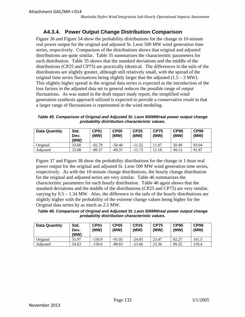
Manitoba Hydro Wind Integration Sub-Hourly Operational Impacts Assessment
A4.3.4. Power Output Change Distribution Comparison Figure 36 and Figure 54 show the probability distributions for the change in 10-minute real power output for the original and adjusted St. Leon 500 MW wind generation time series, respectively. Comparison of the distributions shows that original and adjusted distributions are quite similar. Table 35 summarizes the characteristic parameters for each distribution. Table 35 shows that the standard deviations and the middle of the distributions (CP25 and CP75) are practically identical. The differences in the tails of the distributions are slightly greater, although still relatively small, with the spread of the original time series fluctuations being slightly larger that the adjusted (1.5 – 3 MW). This slightly higher spread in the original data series is expected as the introduction of the loss factors in the adjusted data set in general reduces the possible range of output fluctuations. As was stated in the draft impact study report, the simplified wind generation synthesis approach utilized is expected to provide a conservative result in that a larger range of fluctuations is represented in the wind modeling.
Table 45. Comparison of Original and Adjusted St. Leon 500MWreal power output change probability distribution characteristic values.
Data Quantity Std. Dev. (MW)
CP01 (MW)
CP05 (MW)
CP25 (MW)
CP75 (MW)
CP95 (MW)
CP99 (MW)
Original 33.60 -92.79 -50.40 -11.55 11.07 50.49 93.04 Adjusted 33.08 -89.37 -49.37 -11.73 11.18 49.13 91.87
Figure 37 and Figure 38 show the probability distributions for the change in 1-hour real power output for the original and adjusted St. Leon 500 MW wind generation time series, respectively. As with the 10-minute change distributions, the hourly change distribution for the original and adjusted series are very similar. Table 46 summarizes the characteristic parameters for each hourly distribution. Table 46 again shows that the standard deviations and the middle of the distributions (CP25 and CP75) are very similar, varying by 0.5 – 1.34 MW. Also, the difference in the tails of the hourly distributions are slightly higher with the probability of the extreme change values being higher for the Original data series by as much as 2.5 MW. Table 46. Comparison of Original and Adjusted St. Leon 500MWreal power output change
probability distribution characteristic values.
Data Quantity Std. Dev. (MW)
CP01 (MW)
CP05 (MW)
CP25 (MW)
CP75 (MW)
CP95 (MW)
CP99 (MW)
Original 55.97 -150.9 -91.05 -24.05 23.47 92.27 161.5 Adjusted 54.63 -150.6 -88.83 -23.66 23.36 89.35 159.4
Page 132 3/1/2005
Attachment GAC/MH I-014
November 2013

Manitoba Hydro Wind Integration Sub-Hourly Operational Impacts Assessment
0%
5%
10%
15%
20%
25%
30%
35%
0%
20%
40%
60%
80%
100%
-400 -200 0 200 400
Original 10-Min ChangeFrom 4/1/2003 To 4/1/2004
Electrotek/EPRI PQView®
Count: 52559Min: -450Avg: -0.0007941Max: 450Range: 899.9St Dev: 33.60CP 01: -92.79CP 05: -50.40CP 25: -11.55CP 50: 0CP 75: 11.07CP 95: 50.49CP 99: 93.04SI Range:11.31
Rel
ativ
e F
requ
ency
Cum
ulative Frequency
Delta P All (MW)
Relative Frequency Cumulative Frequency
Figure 53. Probability distribution of change in 10-minute average real power output for ORIGINAL St. Leon 500 MW wind generation time series.
0%
5%
10%
15%
20%
25%
30%
0%
20%
40%
60%
80%
100%
-400 -200 0 200 400
Adjusted - 10-Min ChangeFrom 4/1/2003 To 4/1/2004
Electrotek/EPRI PQView®
Count: 52559Min: -450Avg: 0Max: 450Range: 899.9St Dev: 33.08CP 01: -89.37CP 05: -49.37CP 25: -11.73CP 50: 0CP 75: 11.18CP 95: 49.13CP 99: 91.87SI Range:11.45
Rel
ativ
e F
requ
ency
Cum
ulative Frequency
Delta P All (MW)
Relative Frequency Cumulative Frequency
Figure 54. Probability distribution of change in 10-minute average real power output for ADJUSTED St. Leon 500 MW wind generation time series.
Page 133 3/1/2005
Attachment GAC/MH I-014
November 2013

Manitoba Hydro Wind Integration Sub-Hourly Operational Impacts Assessment
0%
5%
10%
15%
20%
0%
20%
40%
60%
80%
100%
-200 0 200
Original 1-Hr ChangeAvg per Hour, From 4/1/2003 To 4/1/2004
Electrotek/EPRI PQView®
Count: 8759Min: -370Avg: -0.009351Max: 373.3Range: 743.3St Dev: 55.97CP 01: -150.9CP 05: -91.05CP 25: -24.05CP 50: 0CP 75: 23.47CP 95: 92.27CP 99: 161.5SI Range:23.76
Rel
ativ
e F
requ
ency
Cum
ulative Frequency
Delta P All (MW)
Relative Frequency Cumulative Frequency
Figure 55. Probability distribution of change in 1-hour average real power output for ORIGINAL St. Leon 500 MW wind generation time series.
0%
5%
10%
15%
20%
0%
20%
40%
60%
80%
100%
-200 0 200
Adjusted - 1-Hr ChangeAvg per Hour, From 4/1/2003 To 4/1/2004
Electrotek/EPRI PQView®
Count: 8759Min: -362.9Avg: 0.0007794Max: 355.3Range: 718.1St Dev: 54.63CP 01: -150.6CP 05: -88.83CP 25: -23.66CP 50: 0CP 75: 23.36CP 95: 89.35CP 99: 159.4SI Range:23.51
Rel
ativ
e F
requ
ency
Cum
ulative Frequency
Delta P All (MW)
Relative Frequency Cumulative Frequency
Figure 56. Probability distribution of change in 1-hour average real power output for ADJUSTED St. Leon 500 MW wind generation time series.
Page 134 3/1/2005
Attachment GAC/MH I-014
November 2013

Needs For and Alternatives To GAC/MH I‐015
November 2013 Page 1 of 1
REFERENCE: Appendix 9.3 Economic Evaluation Documentation; Section: 1.7; Page 1
No.: 26 2
3
PREAMBLE: Appendix 9.3 notes "The above wind integration costs were flow weighted 4
and then the total divided by the average annual wind generation to produce the unit 5
wind integration costs… The unit wind integration costs are expressed on a marginal 6
basis for each 100 MW increment of wind, and scaled to the current long‐term export 7
price forecast using the ratio of the current long‐term price forecast divided by the 2005 8
price forecast." 9
10
QUESTION: 11
Please provide the work papers for the wind integration cost estimates used in the NFAT filing 12
and specify the basis and source of all assumptions used. 13
14
RESPONSE: 15
In Order 126/13 the PUB determined that it did not require this Information Request to be 16
answered.17

Needs For and Alternatives To GAC/MH I‐016
November 2013 Page 1 of 1
REFERENCE: Appendix 7.4 Capacity Value of Wind Resources; Page No.: 3 1
2
PREAMBLE: Appendix 7.4 indicates "Manitoba Hydro has examined the performance of 3
the existing wind generation fleet in Manitoba during the peak load hour of each month 4
during the period from June 2007 to May 2013. In examining the data set it was found 5
that the minimum wind generation, during the peak load hour each month, was zero or 6
near zero least once each month." 7
8
QUESTION: 9
Please provide the data relied upon and the work papers developed for this analysis. 10
11
RESPONSE: 12
In Order 126/13 the PUB determined that it did not require this Information Request to be 13
answered.14

Needs For and Alternatives To GAC/MH I‐017
November 2013 Page 1 of 3
REFERENCE: Appendix 7.4 Capacity Value of Wind Resources; Page No.: 4 1
2
PREAMBLE: Appendix 7.4 asserts "In consideration of the performance to date of wind 3
generation during the peak monthly load conditions, and the operating requirement to 4
shut down wind generators at ‐30C, when the Manitoba load tends to be peaking, 5
Manitoba Hydro has determined that the capacity value of wind generation within 6
Manitoba to meeting the winter peak load is zero." 7
8
QUESTION: 9
Please provide copies of all analyses performed showing the correlation between Manitoba 10
peak loads and temperature. 11
12
RESPONSE: 13
Please see the table and graph provided below in response to this information request.14

Needs For and Alternatives To GAC/MH I‐017
November 2013 Page 2 of 3
1
Year Date & Time Load (MW) Temp (°C)
2007 1/12/07 8:00 4184 ‐37
2/5/07 8:00 4166 ‐39
1/15/07 8:00 4162 ‐29
1/12/07 17:00 4161 ‐29
1/12/07 18:00 4155 ‐32
2008 12/15/2008 17:00 4396 ‐28
12/15/2008 18:00 4367 ‐28
12/15/2008 19:00 4330 ‐27
12/16/2008 7:00 4304 ‐27
12/15/2008 20:00 4290 ‐27
2009 1/15/2009 8:00 4477 ‐31
1/15/2009 7:00 4434 ‐32
1/14/2009 18:00 4421 ‐29
1/14/2009 19:00 4407 ‐30
1/14/2009 17:00 4398 ‐26
2010 1/7/2010 17:00 4231 ‐23
1/8/2010 8:00 4189 ‐27
1/7/2010 8:00 4179 ‐26
1/7/2010 18:00 4171 ‐25
12/13/2010 8:00 4170 ‐25
2011 1/20/2011 18:00 4262 ‐33
1/20/2011 17:00 4260 ‐32
1/18/2011 18:00 4253 ‐20
1/18/2011 17:00 4235 ‐19
1/18/2011 7:00 4233 ‐35
2012 12/11/2012 17:00 4384 ‐24
1/19/2012 7:00 4343 ‐29
1/19/2012 8:00 4341 ‐29
12/11/2012 18:00 4340 ‐24
12/11/2012 19:00 4321 ‐24
2013 YTD 1/24/2013 8:00 4535 ‐28
to Sept 1/24/2013 7:00 4528 ‐29
1/22/2013 7:00 4526 ‐31
2/1/2013 8:00 4517 ‐29
1/22/2013 8:00 4514 ‐31
2

Needs For and Alternatives To GAC/MH I‐017
November 2013 Page 3 of 3
On average since 1960, there are 101 hours per year where the temperature in Winnipeg is at 1
or below ‐30 C. Manitoba Hydro notes that the calendar years 2009, 2010, 2011 and 2012 have 2
been significantly milder, as measured by the number of hours with a temperature at or below 3
‐30 C, than the long term average with 2012 being the only year in the 50 plus year record of 4
having no hours in the year with temperature in Winnipeg at or below ‐30C. 5
6
7
0
50
100
150
200
250
300
350
400
1960
1962
1964
1966
1968
1970
1972
1974
1976
1978
1980
1982
1984
1986
1988
1990
1992
1994
1996
1998
2000
2002
2004
2006
2008
2010
2012
Hours ‐30 C or Colder
Year
Hours per Year When Winnipeg Temperature was ‐30 C or Colder
Average Hours per Year with ‐30 C or Colder: 101

Needs For and Alternatives To GAC/MH I‐018a
November 2013 Page 1 of 1
REFERENCE: Appendix 7.2 Range of Resource Options; Page No.: 334 1
2
PREAMBLE: Appendix 7.2 indicates that "REC Premium Marketability" for On‐Shore 3
Wind Projects is "Very High" 4
5
QUESTION: 6
Please discuss how REC value is considered in the analysis for any technologies where REC value 7
is assumed. 8
9
RESPONSE: 10
Section 3 of Appendix 7.2 includes the qualitative metric, “REC Premium Marketability” in all resource 11
options in the appendix. Absolute REC values or forecasted REC values were not considered or 12
incorporated into this metric and were not included in Appendix 7.2. 13
14
“REC Premium Marketability” compares the relative REC marketability of individual resource options in 15
comparison to one another. To determine the assessment for individual technologies/projects, the 16
following criterion was considered: 17
18 • Access/eligibility to upper Midwest state‐level RPS markets
19 • Ability for technology to get third party certified (Ecologo/Green‐E)
20 • Specific legislation carve‐outs/explicit preferences for the technology

Needs For and Alternatives To GAC/MH I‐018b
November 2013 Page 1 of 1
REFERENCE: Appendix 7.2 Range of Resource Options; Page No.: 334 1
2
PREAMBLE: Appendix 7.2 indicates that "REC Premium Marketability" for On‐Shore 3
Wind Projects is "Very High" 4
5
QUESTION: 6
Please indicate the source and basis for any assumptions regarding REC value used in the 7
analysis. 8
9
RESPONSE: 10
Please see Manitoba Hydro’s response to GAC/MH I‐018a. 11

Needs For and Alternatives To GAC/MH I‐018c
November 2013 Page 1 of 1
REFERENCE: Appendix 7.2 Range of Resource Options; Page No.: 334 1
2
PREAMBLE: Appendix 7.2 indicates that "REC Premium Marketability" for On‐Shore 3
Wind Projects is "Very High" 4
5
QUESTION: 6
Does Manitoba Hydro realize any Class I REC value for the sale output of the St. Leon and St. 7
Joseph wind projects in US export markets? If not, please discuss why not. 8
9
RESPONSE: 10
Manitoba Hydro does not realize any Class I REC value for the sale output of the St. Leon and St. 11
Joseph wind projects. The St. Leon and St. Joseph wind farm output does not qualify under U.S. 12
state renewable portfolio standards as Class I RECs because the generation is external to the 13
U.S. 14

Needs For and Alternatives To GAC/MH I‐019a
November 2013 Page 1 of 1
REFERENCE: Appendix 9.1 High Level Development Plan Comparison Table; 1
2
PREAMBLE: The High Level Development Plan Comparison Table indicates that the 3
Wind/Gas plan would require transmission development of 943 Km. 4
5
QUESTION: 6
Please provide the basis for the estimated length of transmission lines and indicate the rated 7
capacity of these lines. Please specify all assumptions and the basis for these assumptions. 8
9
RESPONSE: 10
The following table provides a breakdown of the estimated transmission length required for the 11
Wind/Gas development plan. The breakdown assumes that the best wind resource locations 12
will be developed first and that the required transmission would be developed in coordinated 13
stages. 14
15
Transmission Linear Development
3
ComponentTransmission Length (km)
Line Rating
Wind/Gas
Thermal - Stage 1 40 230 kV 40Thermal - Stage 2 40 230 kV 40Wind - Stage 1 163 230 kV 163Wind - Stage 2 350 230 kV 350Wind - Stage 3 350 230 kV 350
Total Length 943

Needs For and Alternatives To GAC/MH I‐019b
November 2013 Page 1 of 1
REFERENCE: Appendix 9.1 High Level Development Plan Comparison Table 1
2
PREAMBLE: The High Level Development Plan Comparison Table indicates that the 3
Wind/Gas plan would require transmission development of 943 Km. 4
5
QUESTION: 6
Does the length of required transmission assume that there will be a coordinated buildout of 7
the transmission network, with facilities sized to accommodate future projects that are 8
anticipated to be built in the area? Please discuss. 9
10
RESPONSE: 11
It is assumed that the transmission infrastructure required to connect the different resources 12
would be constructed in a manner that minimizes long term costs. Individually CCGT, SCGT and 13
wind are small modular units that in some development plans require multiple units to be 14
installed over time. In these cases it is assumed that transmission will be constructed in a 15
staged and coordinated manner over the long term. 16

Needs For and Alternatives To GAC/MH I‐019c
November 2013 Page 1 of 1
REFERENCE: Appendix 9.1 High Level Development Plan Comparison Table 1
2
PREAMBLE: The High Level Development Plan Comparison Table indicates that the 3
Wind/Gas plan would require transmission development of 943 Km. 4
5
QUESTION: 6
Please estimate the incremental capital requirements on a NPV basis for the 943 Km of 7
transmission required for this development plan. 8
9
RESPONSE: 10
As shown in Tables 009 and 010 of Appendix 9.3 the present value of the incremental 11
transmission capital required for the Wind/Gas development plan compared to the All Gas 12
development plan is $225 million ([email protected]%). 13
14
Wind/Gas – Transmission Capital NPV $375 million 15
All Gas – Transmission Capital NPV ‐ $150 million 16
Incremental Transmission Capital NPV $225 million ([email protected]%) 17

Needs For and Alternatives To GAC/MH I‐020a
November 2013 Page 1 of 1
REFERENCE: Appendix 9.1 High Level Development Plan Comparison Table; 1
2
PREAMBLE: The High Level Development Plan Comparison Table indicates that the 3
mode of operation will be must take and peaking, reflecting that the development plan 4
assumes a combination of wind and SCGTs. 5
6
QUESTION: 7
Did Manitoba Hydro evaluate the economics of a wind and CCGT development plan? If not, 8
please discuss. 9
10
RESPONSE: 11
Manitoba Hydro did not evaluate the economics of a wind and CCGT development plan. 12
13
The Wind/Gas development plan presented in the NFAT Business Case represents a 14
development plan that maximizes the amount of wind energy available with the lowest capital 15
investment resource to provide capacity support for the wind resources. Due to the expected 16
dispatch of a natural gas‐fired generation resource to support of the intermittent energy 17
resource of significant new wind generation, SCGTs were included in the development plan as 18
the expected overall capacity factor of the fleet of SCGTs is typical of peaking resources. 19
20
For the Wind/Gas development plan, based on a preliminary analysis of expected capacity 21
factor of SCGTs in this plan, usage of the SCGTs would not reach the typical capacity factor of a 22
CCGT until the 2040 timeframe. 23

Needs For and Alternatives To GAC/MH I‐020b
November 2013 Page 1 of 1
REFERENCE: Appendix 9.1 High Level Development Plan Comparison Table; 1
2
PREAMBLE: The High Level Development Plan Comparison Table indicates that the 3
mode of operation will be must take and peaking, reflecting that the development plan 4
assumes a combination of wind and SCGTs. 5
6
QUESTION: 7
Did Manitoba Hydro evaluate the economics of a wind/gas development plan where the mix of 8
generation resources was varied depending on market conditions, e.g., greater reliance of 9
CCGTs when gas costs are high or when the cost of carbon is high? If not, please discuss. 10
11
RESPONSE: 12
Manitoba Hydro did not evaluate the economics of any of its development plans where the mix 13
of generation resources would be varied depending on market conditions. Please see Manitoba 14
Hydro’s response to GAC/MH I‐20a. 15
16
Please also see Chapter 14 Figure 14.2 for a depiction of pathways which considers a change in 17
generation resources depending on circumstances. 18

Needs For and Alternatives To GAC/MH I‐020c
November 2013 Page 1 of 1
REFERENCE: Appendix 9.1 High Level Development Plan Comparison Table 1
2
PREAMBLE: The High Level Development Plan Comparison Table indicates that the 3
mode of operation will be must take and peaking, reflecting that the development plan 4
assumes a combination of wind and SCGTs. 5
6
QUESTION: 7
Did Manitoba Hydro evaluate greater reliance on demand response programs in the wind/gas 8
development plan to reduce the reliance on natural gas capacity requirements? Please discuss. 9
10
RESPONSE: 11
Manitoba Hydro did not evaluate greater reliance on Demand Response programs in the 12
wind/gas development plan for the purpose of reducing reliance on natural gas capacity 13
requirements. At present, Manitoba Hydro’s Curtailable Rates program is the only demand 14
response program included in the portfolio of DSM options included in this NFAT filing. The 15
capacity reductions provided by this program are not included for purposes of long‐term 16
capacity planning (please see Manitoba Hydro’s response to MIPUG/MH I‐24a and 17
CAC_GAC/MH I‐030b. 18
19
Utilization of demand response capability to firm wind resources requires careful consideration 20
of the frequency, duration and criticality of the intermittency in wind resources. Demand 21
response programs are generally intended to relieve capacity constraints during shorter 22
duration (hours) periods of peak system loading, which may not always correlate well to the 23
firm requirement for energy during the peak consumption periods caused by extreme cold 24
when wind is often not available for sustained (days) periods. 25

Needs For and Alternatives To GAC/MH I‐021
November 2013 Page 1 of 1
REFERENCE: Business Case 1
2
QUESTION: 3
Please provide, in electronic format, the hourly profiles of wind generation used in modelling. 4
The profiles may be normalized or scaled in any way that is convenient as the focus of this IR is 5
the variability and seasonality of wind generation, not its absolute level. 6
7
RESPONSE: 8
Manitoba Hydro does not use an hourly wind profile in its long‐term resource planning process. 9
Instead, it uses monthly energy profile factors, provided below, which can be applied to the 10
average monthly wind facility output, to create a monthly energy profile. 11
12
Apr 1.10
May 1.03
Jun 0.93
Jul 0.83
Aug 0.87
Sep 0.97
Oct 1.00
Nov 1.08
Dec 1.07
Jan 1.03
Feb 1.03
Mar 1.07

Needs For and Alternatives To GAC/MH I‐022
November 2013 Page 1 of 1
REFERENCE: Business Case 1
2
QUESTION: 3
Please provide, in electronic format, recorded hourly temperature readings in the locations 4
where wind is assumed to be developed in one or more scenarios. The source could either be 5
Environment Canada for a nearby location, or site‐specific measurements, and should extend 6
over as many years as possible. 7
8
RESPONSE: 9
Manitoba Hydro is unable to provide temperature data specific to locations of proposed wind 10
developments. New wind generation resources considered in the NFAT Business Case are 11
generally assumed to be developed in Southern Manitoba, in areas with higher wind speeds as 12
indicated by Appendix 7.1 Figure 4. Available temperature data in these general areas is 13
downloadable via the following Environment Canada website link: 14
http://climate.weather.gc.ca/prods_servs/attachment1_e.html 15
16
Please also see Manitoba Hydro’s response to GAC/MH I‐017 which provides a chart showing 17
the number of hours per year since 1960 where the temperature in Winnipeg is at or below ‐30 18
C.19

Needs For and Alternatives To GAC/MH I‐023
November 2013 Page 1 of 1
REFERENCE: Business Case 1
2
QUESTION: 3
Please provide, in electronic format, hourly grid‐connected demand in Manitoba over at least 4
the last five years. Please exclude exports, and demand in remote communities served by 5
isolated diesel generators. Please specify whether the data provided is at the customer level or 6
the system level ‐ i.e., before or after transmission and distribution losses. No breakdown by 7
geographic area or by customer types is required. 8
9
RESPONSE: 10
In Order 119/13 the PUB determined that it did not require the Information Request to be 11
answered.12

Needs For and Alternatives To GAC/MH I‐024
November 2013 Page 1 of 1
REFERENCE: Business Case 1
2
QUESTION: 3
Please provide, in electronic format, the hourly load shape or shapes used to model Manitoba 4
electricity demand. The data may be normalized or scaled, as the focus of this IR is on variability 5
and seasonality, not on absolute levels of demand. 6
7
RESPONSE: 8
In Order 119/13 the PUB determined that it did not require the Information Request to be 9
answered.10
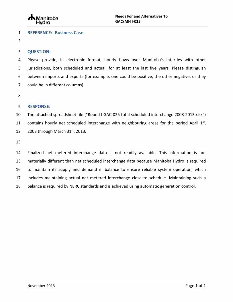
Needs For and Alternatives To GAC/MH I‐025
November 2013 Page 1 of 1
REFERENCE: Business Case 1
2
QUESTION: 3
Please provide, in electronic format, hourly flows over Manitoba's interties with other 4
jurisdictions, both scheduled and actual, for at least the last five years. Please distinguish 5
between imports and exports (for example, one could be positive, the other negative, or they 6
could be in different columns). 7
8
RESPONSE: 9
The attached spreadsheet file (“Round I GAC‐025 total scheduled interchange 2008‐2013.xlsx”) 10
contains hourly net scheduled interchange with neighbouring areas for the period April 1st, 11
2008 through March 31st, 2013. 12
13
Finalized net metered interchange data is not readily available. This information is not 14
materially different than net scheduled interchange data because Manitoba Hydro is required 15
to maintain its supply and demand in balance to ensure reliable system operation, which 16
includes maintaining actual net metered interchange close to schedule. Maintaining such a 17
balance is required by NERC standards and is achieved using automatic generation control. 18

Needs For and Alternatives To GAC/MH I‐026
November 2013 Page 1 of 3
REFERENCE: Business Case 1
2
QUESTION: 3
Please provide, in electronic format, monthly summaries of electric energy supply to the 4
Manitoba grid for at least the last five years, broken down into categories including hydro, 5
thermal, wind, and imports. Please exclude supply to remote communities served by isolated 6
diesel generators. 7
8
RESPONSE: 9
Table 1 shows monthly energy supply broken down into the following categories: Hydraulic, 10
Thermal, and the sum of Wind and Imports. Monthly wind generation data is confidential so it 11
has been aggregated with imports. Manitoba Hydro has been unable to get the consent of the 12
wind farm owner to release un‐aggregated wind generation data. 13

Needs For and Alternatives To GAC/MH I‐026
November 2013 Page 2 of 3
1
Table 1. Monthly Energy Supply in GWh.
Month‐Year Hydraulic Thermal Wind + Imports
Apr‐08 2,693 41 43 May‐08 2,673 0 29 Jun‐08 2,530 5 30 Jul‐08 3,059 36 27 Aug‐08 3,150 56 29 Sep‐08 2,976 1 31 Oct‐08 3,024 25 40 Nov‐08 3,018 49 43 Dec‐08 2,886 57 144 Jan‐09 2,889 56 125 Feb‐09 2,602 2 44 Mar‐09 2,694 7 88
Apr‐09 2,571 25 43 May‐09 2,727 0 43 Jun‐09 2,675 0 40 Jul‐09 2,948 4 33 Aug‐09 2,932 8 26 Sep‐09 2,750 6 35 Oct‐09 3,163 8 30 Nov‐09 2,863 33 55 Dec‐09 2,840 33 145 Jan‐10 2,938 7 138 Feb‐10 2,621 6 66 Mar‐10 2,790 13 32
Apr‐10 2,499 6 33 May‐10 2,001 7 160 Jun‐10 2,498 6 26 Jul‐10 2,976 4 25 Aug‐10 3,048 8 29 Sep‐10 2,816 1 36 Oct‐10 3,026 7 37 Nov‐10 3,030 3 42 Dec‐10 3,125 4 57
Jan‐11 3,081 19 63 Feb‐11 2,802 3 66 Mar‐11 3,132 0 56
2

Needs For and Alternatives To GAC/MH I‐026
November 2013 Page 3 of 3
1
Table 1 (continued). Monthly Energy Supply in GWh.
Month‐Year Hydraulic Thermal Wind + Imports
Apr‐11 2,782 11 60 May‐11 2,840 3 91 Jun‐11 2,687 5 68 Jul‐11 3,191 8 51 Aug‐11 3,043 11 56 Sep‐11 2,536 6 89 Oct‐11 2,696 11 91 Nov‐11 2,735 13 118 Dec‐11 2,783 2 141 Jan‐12 2,904 3 137 Feb‐12 2,500 2 165 Mar‐12 2,461 3 179
Apr‐12 2,226 4 141 May‐12 2,466 0 107 Jun‐12 2,565 1 94 Jul‐12 3,184 1 46 Aug‐12 3,129 2 60 Sep‐12 2,715 0 80 Oct‐12 2,549 24 112 Nov‐12 2,727 12 119 Dec‐12 2,859 3 198 Jan‐13 2,987 8 215 Feb‐13 2,696 2 125 Mar‐13 3,044 1 83

Needs For and Alternatives To GAC/MH I‐027a
November 2013 Page 1 of 1
REFERENCE: Chapter 6: The Window of Opportunity 1
2
PREAMBLE: Chapter 6, p. 22, Table 6.3 (bottom right cell): "Hydropower can usually 3
start and ramp up output quickly. In some systems, hydropower is the best option for 4
regulation up and a major source of regulation down as well as spinning reserve. 5
Appropriate energy and operating reserve pricing is necessary to ensure appropriate 6
investment in new generation technologies for hydropower to be available to provide 7
services important for the integration of other sources of renewable energy." 8
9
QUESTION: 10
Please describe the "new generation technologies for hydropower" which can "provide services 11
important for the integration of other sources of renewable energy." 12
13
RESPONSE: 14
The quoted statement “appropriate energy and operating reserve pricing is necessary to ensure 15
appropriate investment in new generation technologies for hydropower to be available to 16
provide services important for the integration of other sources of renewable energy” is made in 17
the broad context of power systems/ markets, rather than specific comment pertaining to the 18
Manitoba Hydro situation. The reference to new generation technologies for hydropower 19
relates to advanced pumped storage units, and variable speed pump storage units as well as 20
“ternary” combinations of turbine, generator, torque converter and multi‐stage pump10. In 21
some power systems, such new technology would be beneficial to support the integration of 22
large amounts of variable generation such as wind generation. 23
10 A Comparison of Advanced Pumped Storage Equipment Drivers in the US and Europe, by Richard K. Fisher and others, 2012.

Needs For and Alternatives To GAC/MH I‐027b
November 2013 Page 1 of 1
REFERENCE: Chapter 6: The Window of Opportunity 1
2
PREAMBLE: Chapter 6, p. 22, Table 6.3 (bottom right cell): "Hydropower can usually 3
start and ramp up output quickly. In some systems, hydropower is the best option for 4
regulation up and a major source of regulation down as well as spinning reserve. 5
Appropriate energy and operating reserve pricing is necessary to ensure appropriate 6
investment in new generation technologies for hydropower to be available to provide 7
services important for the integration of other sources of renewable energy." 8
9
QUESTION: 10
Have Keeyask and Conawapa been designed to provide such integration services? If not, why 11
not? 12
13
RESPONSE: 14
As indicated in the response to GAC/MH I‐027a, the reference to new generation technologies 15
was made in the broad context of power systems/markets, rather than a specific comment 16
pertaining to the Manitoba Hydro situation. The specific technologies referenced are related to 17
advanced pumped storage units. Keeyask and Conawapa are not designed as pumped storage 18
plants. The upstream reservoirs will be continuously replenished as they are part of the Nelson 19
River. The use of other energy sources to provide energy to pump water into the upstream 20
reservoirs is not required. 21
22
Like Manitoba Hydro’s existing generation, Keeyask and Conawapa will be capable of 23
supporting wind integration. 24

Needs For and Alternatives To GAC/MH I‐027c
November 2013 Page 1 of 1
REFERENCE: Chapter 6: The Window of Opportunity 1
2
PREAMBLE: Chapter 6, p. 22, Table 6.3 (bottom right cell): "Hydropower can usually 3
start and ramp up output quickly. In some systems, hydropower is the best option for 4
regulation up and a major source of regulation down as well as spinning reserve. 5
Appropriate energy and operating reserve pricing is necessary to ensure appropriate 6
investment in new generation technologies for hydropower to be available to provide 7
services important for the integration of other sources of renewable energy." 8
9
QUESTION: 10
Compare the feasibility and costs of a subsequent retrofit of existing generating stations with 11
"new generation technologies for hydropower" vs. designing and installing these technologies 12
at the point of new construction. 13
14
RESPONSE: 15
It would be very difficult to convert an existing conventional hydro generating station to a 16
pumped storage plant. However, there is no reason to consider such a conversion of Manitoba 17
Hydro’s facilities. While pumped storage can be a useful technology to assist with system 18
optimization and wind integration, particularly in power systems with large amounts of 19
baseload generation such as nuclear power, pumped storage is not required to integrate wind 20
generation In Manitoba. 21
22
Manitoba Hydro’s existing generation, and the proposed Keeyask and Conawapa generating 23
stations, are / will be capable of supporting wind integration. 24

Needs For and Alternatives To GAC/MH I‐027d
November 2013 Page 1 of 1
REFERENCE: Chapter 6: The Window of Opportunity 1
2
PREAMBLE: Chapter 6, p. 22, Table 6.3 (bottom right cell): "Hydropower can usually 3
start and ramp up output quickly. In some systems, hydropower is the best option for 4
regulation up and a major source of regulation down as well as spinning reserve. 5
Appropriate energy and operating reserve pricing is necessary to ensure appropriate 6
investment in new generation technologies for hydropower to be available to provide 7
services important for the integration of other sources of renewable energy." 8
9
QUESTION: 10
How is MH preparing to deliver a firming and integrating product as an alternative to baseload 11
power in Manitoba and MISO? 12
13
RESPONSE: 14
Manitoba Hydro is not preparing to deliver a firming and integrating product as an alternative 15
to baseload power. 16
17
As described in Chapter 5, pages 21 and 22, Manitoba Hydro has the ability to store energy by 18
maintaining and increasing forebay levels at various generating stations. This capability allows 19
Manitoba Hydro to meet a portion of its off‐peak domestic load requirements by importing 20
energy from external markets during less expensive hours and returning the energy to these 21
external markets during the more profitable on‐peaks hours the next day. The ability of 22
Manitoba Hydro’s generation facilities to act as a storage battery is particularly valuable in light 23
of the substantial wind development occurring in MISO and across the US and the fact that a 24
significant proportion of energy generated by those wind resources occurs during off‐peak 25
hours when there is low demand in MISO and can be exported inexpensively to entities like 26
Manitoba Hydro. 27

Needs For and Alternatives To GAC/MH I‐028
November 2013 Page 1 of 1
REFERENCE: Overview ‐ Meeting Manitobans' Electricity Needs; Page No.: p. 5 1
2
PREAMBLE: Overview, p. 5 states: "12 Minimal Downside Risk 13 Manitoba Hydro has 3
the ability to cancel the new export sale contracts should new generation 14 and/or 4
transmission facilities in Manitoba not be approved." 5
6
QUESTION: 7
Do the counterparties have the ability to cancel the new export sale contracts if Manitoba 8
Hydro finds that it can supply dispatchable hydropower to fulfill the contracts without building 9
new hydro generating stations by, for example, aggressive DSM and demand response? Is the 10
linking of the contracts to new construction solely a stipulation of Manitoba Hydro? Discuss. 11
12
RESPONSE: 13
No. The contracts are tied to the development of major new hydro generating resources with 14
associated renewable attributes. 15
Manitoba Hydro is unique in being able to offer a large dispatchable hydro supply option to its 16
export customers. Other Manitoba Hydro options are not of interest to Manitoba Hydro 17
counterparties because they have their own supply options such as wind, natural gas or DSM, 18
which can be developed locally at a lower cost than from Manitoba. 19

Needs For and Alternatives To GAC/MH I‐029a
November 2013 Page 1 of 2
REFERENCE: Sept 5. Transcript; Page No.: 43‐44 1
2
PREAMBLE: At the September 5 Technical Conference Transcript, pp. 43‐44, Lois 3
Morrison states that Manitoba Hydro does not factor price elasticity into its forecasts. 4
5
QUESTION: 6
Please provide Manitoba Hydro's response to RCM/TREE/MH II‐26(b) in the 2005‐2006 Cost of 7
Service hearing, comment on the elasticity studies cited therein, and indicate whether or not 8
(and why) they are relevant to forecasts under rapidly escalating rates such as are projected for 9
the next two decades in Manitoba. 10
11
RESPONSE: 12
Please find RCM/TREE/MH II‐26(b) from the 2005/06 Cost of Service hearing as an attachment 13
to this response. That response cites two studies, a Danish study that investigated how 14
company characteristics influence price and production elasticities, and a review by the 15
Bonneville Power Administration that documents historic and current estimates of price 16
elasticities for residential, commercial and industrial classes. 17
18
The Danish study was based on a panel of 2,949 Danish industrial companies. This study found 19
that price elasticities varied by industrial sub‐sectors and by electricity intensity in production. 20
The Danish study found that industrial companies with more electricity intensive operations 21
would be more responsive to changes in the electricity price. 22
23
The second study cited provided then‐current and historical estimates of short‐run and long‐24
run price elasticities for various customer classes. The study results indicated that long‐run 25
elasticities are higher than short‐run elasticities. For the utilities included in the study, price 26

Needs For and Alternatives To GAC/MH I‐029a
November 2013 Page 2 of 2
changes would cause a more significant impact to electricity demand in the intermediate and 1
long term. 2
3
The findings in these studies provide the following insights: while in the initial years of rate 4
increases electricity usage may not be as responsive to the increase in price, the impact on 5
electricity demand may be larger in the longer term. Secondly, electricity demand of industrial 6
customers that are more electricity intensive in production would be more responsive to the 7
price increases. 8
9
It is important to note that estimates of price elasticity vary from study to study, and this 10
variation is driven by factors such as the region under study, price levels, data aggregation, time 11
periods of analysis and the methodology of estimation used. Consequently, the results of the 12
various studies, while informative, may not necessarily be directly transferable to the Manitoba 13
market.14

RCM/TREE/MH II-26 Subject: Price elasticity and substitutes Reference: RCM/TREE/MH 1-4(d) b) Does MH believe that elasticities in the range of –0.2 to –0.4 are appropriate for
all classes on its system, or does it have information that certain classes or certain elements of demand are less or more elastic than others? Provide recent elasticity analysis if it is relevant to this inquiry including the response to MIPUG/MH II-9(d) from the 2004 GRA hearing.
ANSWER:
Manitoba Hydro cannot confirm that elasticities in the range cited actually apply to any or all
classes on its system. However, they are plausible, and reasonably inferred from other
studies of elasticity in other jurisdictions. One can always find contrary results, but the
weight of evidence appears to be that industrial uses are more elastic than commercial which
are, in turn, more elastic than residential. Within industrial classes, those customers for
whom electricity is a significant share of the cost of production likely have demands which
are more elastic than those for whom electricity makes up only a small share of the cost of
production.
Within the Residential class it is likely that some end uses have more demand elasticity than
others. Lighting, most appliances and small motors probably have very low elasticity, since
there is no real substitute for electricity for these uses. Space and water heating and, perhaps
air conditioning, may have higher elasticity since alternate fuels can be purchased and
customers may be prepared to accept a lower degree of physical comfort if prices increase
significantly.
The response to MIPUG/MH II-9(d) from the 2004 GRA hearing has been replicated and
included as an attachment to this response.
2006 03 02 Page 1 of 1
Attachment GAC/MH I-029a
November 2013

ATTACHMENT RCM-TREE/MH II-26(b)
MIPUG/MH II-9
Reference: PUB/MH I -43
d) Please provide any studies or analysis done by Manitoba Hydro to quantify theelasticity of industrial loads with respect to electricity costs.
ANSWER:
Manitoba Hydro has not undertaken its own research into the elasticity of industrial
electricity demand with respect to prices. Generally speaking, it would be expected that the
greater the percentage electricity costs make up of the overall budget of any customer,
residential, commercial or industrial, the more sensitive that customer’s demand will be to
the price of electricity. Thus one would expect households using or contemplating electricity
for home heating would be more sensitive to the price of electricity than households which
do not. Similarly, electricity-intensive industry would be expected to be more influenced in
location or expansion decisions by the price of electricity than other industry for which
electricity constitutes only a small portion of the cost of production. This appears to be borne
out in the experience in Manitoba with respect to load expansion of various industries and
residential and commercial loads discussed in the response to MIPUG/MH II-9(e).
A Danish study, a copy of which is attached as Appendix 41, appears to bear out this
conclusion. The study followed a panel of 2,949 Danish companies from 1983 to 1996. It
investigated, among other issues, how various company characteristics such size, type of
industrial sub-sector, and electricity intensity in production influence price and production
elasticities. It appears that companies with a high electricity intensity also have a high own-
price elasticity. Average industrial elasticity determined in this study was -0.479.
There exists a very significant body of literature on the subject of price elasticity of demand
for electricity and results vary considerably depending on the location, the time periods of
analysis, the methodology of estimation used and other factors. A review by Bonneville
Power Authority (go to www.bpa.gov/Power/LP/sn03/files/Parties Data Responses/CR-WA-004A.doc) documents historic and current estimates of price elasticities for residential,
commercial and industrial customer classes. Historic estimates of short run price elasticity
show a range of -0.13 to -0.45 for Residential; -0.17 to -0.42 for Commercial and -0.30 to
-0.59 for Industrial. Short run elasticities based on more current studies show a range of -
0.20 to -0.44 for Residential; -0.12 to -0.38 for Commercial and -0.39 to -0.69 for Industrial.
2004 05 17 Page 1 of 2
Attachment GAC/MH I-029a
November 2013

ATTACHMENT RCM-TREE/MH II-26(b)
Long run elasticities based on more current studies range from -0.35 to -2.23 for Residential;
-0.29 to -1.65 for Commercial and -0.76 to -2.87 for Industrial.
2004 05 17 Page 2 of 2
Attachment GAC/MH I-029a
November 2013

Needs For and Alternatives To GAC/MH I‐029b
November 2013 Page 1 of 1
REFERENCE: Sept 5. Transcript; Page No.: 43‐44 1
2
PREAMBLE: At the September 5 Technical Conference Transcript, pp. 43‐44, Lois 3
Morrison states that Manitoba Hydro does not factor price elasticity into its forecasts. 4
5
QUESTION: 6
Please provide the transcripts of Mr. Kuczek's 2008 GRA testimony on March 3, pp. 94‐95 and 7
March 10, pp. 741‐744 comparing Saskatchewan's decline with Manitoba's increase in electrical 8
consumption. 9
10
RESPONSE: 11
Please see the attachment to this response. 12

Page 93
research, for developing a load forecast, for consu --1
customer services provided through the Corporation's2
customer contact centre, and for customer service3
extension services.4
MS. PATTI RAMAGE: Could you please5
comment on the nature of Manitoba Hydro's energy6
conservation program?7
MR. LLOYD KUCZEK: Manitoba Hydro8
currently offers one of the most aggressive and9
longstanding commitments to DSM in North America. 10
Manitoba Hydro has been offering energy conservation11
programs since 1989, and the Corporation has12
significantly ramped up its efforts over the years to13
capture energy effic -- efficiency opportunities. 14
Mani -- Manitoba Hydro's DSM efforts are15
consistent with industry best practices and compare --16
compare favourably to programs being offered by leading-17
edge North American utilities and agencies.18
MS. PATTI RAMAGE: Can you comment on how19
you can support this position?20
MR. LLOYD KUCZEK: I use an aggregate of21
indicators and sources to support my assessment, which22
include the Canadian Energy Efficiency Alliances23
Evaluation of regional actions taken towards achieving24
energy efficiency in Canada. This analysis is undertaken25
Attachment GAC/MH I-029b
November 2013

Page 94
by an independent party and involves a comprehensive and1
broad assessment, including the evaluation of twelve (12)2
parameters. This organization provided Manitoba with an3
"A" rating, which was the highest rating in Canada, for4
the past two (2) assessments. 5
Manitoba Hydro also received the Energy6
Star Utility of the Year Award in recognition of their7
promotion of the Energy Star brand. 8
Manitoba Hydro also received a number of9
program-specific awards and other recognition indicators,10
including phone calls from peers working at other11
utilities inquiring about our leading-edge programs.12
Manitoba Hydro's comprehensive approach to13
pursuing energy efficiency opportunities, including14
offering convenient financial support services and15
working with the government at on -- excuse me -- on an16
overall market transformation strategy will -- that will17
ensure sustainability of energy efficiency. 18
Also, I use comparative information19
received on -- on various energy efficiency efforts being20
offered by leading edge -- leading energy conservation21
organizations through North America, including22
information received through conference calls involving23
num -- numerous entities in North America and high-level24
comparative data provided by the Consortium of Energy25
Attachment GAC/MH I-029b
November 2013

Page 95
Efficiency, which provided -- provides data on energy1
efficiency budgets on a per capita basis for US and2
Canadian regions. 3
In the most recent report Manitoba Hydro4
was rated as the -- rated the highest in this category5
for efforts targeting electricity for all regions in6
North America. 7
And also added to that, SaskPower recently8
contracted with Manitoba Hydro to help them develop their9
energy efficiency plan.10
MS. PATTI RAMAGE: And thank you, Mr.11
Kuczek. Can you provide any comments about Manitoba12
Hydro's low-income program?13
MR. LLOYD KUCZEK: This program was just14
recently launched, and we recognize that there will be15
many challenges in ensuring that this program is16
effective for both lower-income Manitobans and Manitoba17
Hydro. 18
The Corporation, however, is confident19
that the program will be successful, and it is Manitoba20
Hydro's intent to make adjustments to the program as21
deemed appropriate.22
MS. PATTI RAMAGE: Thank you, Mr. Kuczek. 23
And with that, I can present this panel of witnesses to24
Mr. Peters for cross-examination. We have a lot of25
Attachment GAC/MH I-029b
November 2013

Page 741
sentence on that page at Tab 33 of the book of documents1
under 4.3.2.5 where it indicates that: 2
"the calculation of cents per kilowatt3
hour saved was based upon current4
program kilowatt hour savings, a5
generation over a thirty (30) year6
planning period."7
MR. LLOYD KUCZEK: Yes. So -- so what8
that means and I could be corrected by the person behind9
me but, as I understand it, what we -- once you get the10
savings in those -- that year or the -- in the years up11
to the year of the evaluation, you assume that you're12
going to have those savings going forward.13
It does not assume you're going to get14
future energy savings which you are expecting to get in15
the -- in the future years of the program.16
MR. BOB PETERS: All right. Well thank17
you for that clarification. At Tab 34 of the book of18
documents the total resource cost test results were19
published for various DSM projects. 20
Would the Board be correct in concluding21
that there is no benefit included in the total resource22
cost test for delayed generation?23
MR. LLOYD KUCZEK: That's correct.24
MR. BOB PETERS: When we look at demand25
Attachment GAC/MH I-029b
November 2013

Page 742
side management and compare Manitoba with Saskatchewan,1
would you agree that in both provinces for the non all-2
electric homes there's roughly ten thousand (10,000)3
kilowatt hours per year used as an average amount?4
MR. LLOYD KUCZEK: It's in that range,5
yes.6
MR. BOB PETERS: And would it also be in7
that range that Saskatchewan's consumption is declining8
by approximately 2.9 percent per year?9
MR. LLOYD KUCZEK: I believe one (1) of10
the IRs responded to that. I don't recall exactly the --11
the percentage decline.12
MR. BOB PETERS: My -- my note was13
PUB/Hydro First Round question 94 but if Manitoba -- if14
Saskatchewan's consumption was declining by about 2.915
percent a year, Manitoba's consumption appears to be16
increasing by just over 7 percent a year, correct?17
MR. LLOYD KUCZEK: Yes, ours is18
increasing and I think as part of that response we19
explained that it was related to the increased20
electric/waterload that we're incurring and it's not21
happening in Saskatchewan.22
MR. BOB PETERS: Maybe you could explain23
that to the Board. 24
What you -- what you're trying to suggest25
Attachment GAC/MH I-029b
November 2013

Page 743
to the Board is that in the province to our west their1
annual electricity consumption is decreasing by about 32
percent a year but in Manitoba it's increasing by 73
percent a year and Manitoba Hydro believes that's4
probably related to increased use of electric hot water5
heat?6
MR. LLOYD KUCZEK: Yes, and I should I7
guess -- you -- you mentioned earlier that the average8
use for a home heated with electricity is about ten9
thousand (10,000) kilowatt hours. I don't know that's10
correct in Saskatchewan. I suspect it's much lower than11
that because the market there is not using, as I12
understand it, electric hot water tanks, it's using13
primarily natural gas.14
MR. BOB PETERS: And in Manitoba there's15
a movement to use electricity to heat hot water, or I16
guess to heat water, primarily because there's no need17
for a chimney if you use electric hot water heaters18
rather than gas?19
MR. LLOYD KUCZEK: Yeah, it's the overall20
cost associated with installing a natural gas hot water21
tank relative to electric hot water tank that is shipped22
at the market in Manitoba and, yes, you do not need a23
chimney so the new home construction practice has moved24
towards not including chimneys in their designs anymore.25
Attachment GAC/MH I-029b
November 2013

Page 744
MR. BOB PETERS: And that's primarily1
because even if you heat with -- with natural gas a high-2
efficiency natural gas furnace doesn't need a chimney?3
MR. LLOYD KUCZEK: Correct.4
MR. BOB PETERS: And if you don't need a5
chimney for your furnace, it would be perceived as6
expensive to put in a chimney just for the purposes of7
venting a natural gas hot water tank?8
MR. LLOYD KUCZEK: Yes.9
MR. BOB PETERS: In terms of Manitoba10
Hydro's DSM program and the City of Winnipeg agreement11
that they have, not only was there a requirement for a12
new Manitoba Hydro headquarters built in the City of13
Winnipeg but there was also an agreement where Manitoba14
Hydro would help the City with its demand side management15
programs; correct?16
MR. LLOYD KUCZEK: Correct.17
MR. BOB PETERS: There was an expectation18
that Manitoba Hydro could help the City of Winnipeg save19
eight hundred thousand dollars ($800,000) a year to20
partially defray the cost of Mr. Doug Buhr's salary?21
MR. LLOYD KUCZEK: There -- there was a22
commitment to achieve them eight hundred thousand dollars23
($800,000) in energy savings a year, a minimum of that,24
yes. 25
Attachment GAC/MH I-029b
November 2013
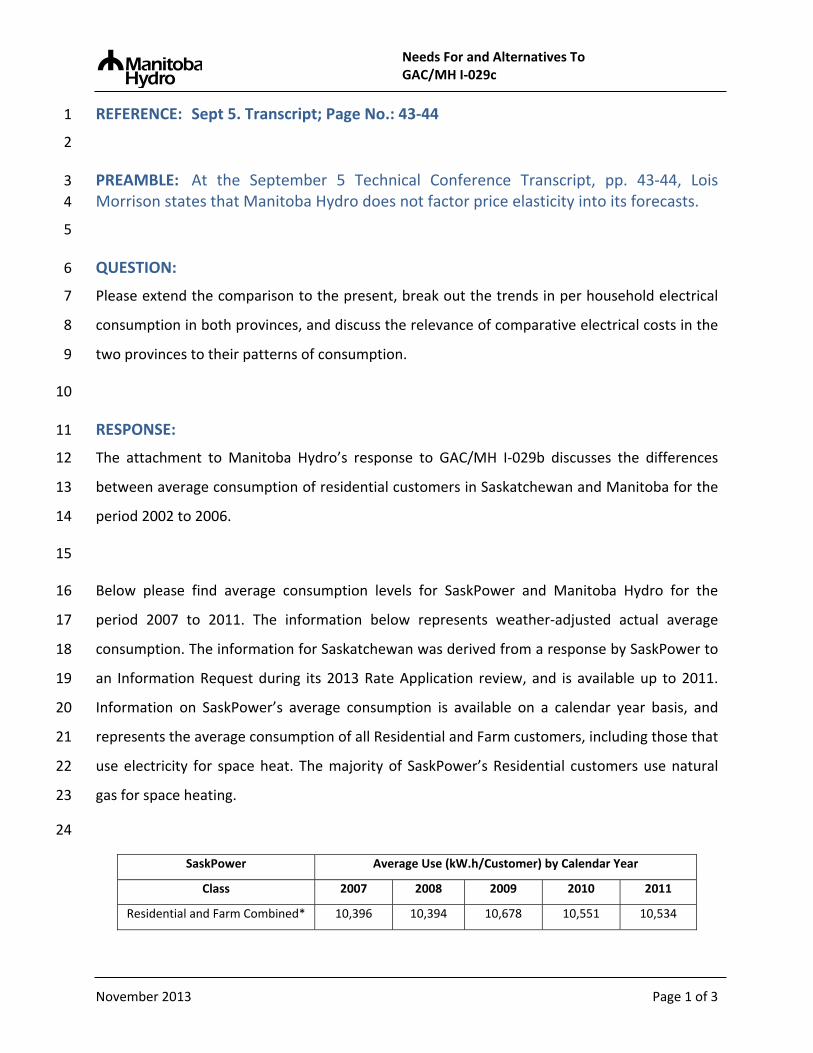
Needs For and Alternatives To GAC/MH I‐029c
November 2013 Page 1 of 3
REFERENCE: Sept 5. Transcript; Page No.: 43‐44 1
2
PREAMBLE: At the September 5 Technical Conference Transcript, pp. 43‐44, Lois 3
Morrison states that Manitoba Hydro does not factor price elasticity into its forecasts. 4
5
QUESTION: 6
Please extend the comparison to the present, break out the trends in per household electrical 7
consumption in both provinces, and discuss the relevance of comparative electrical costs in the 8
two provinces to their patterns of consumption. 9
10
RESPONSE: 11
The attachment to Manitoba Hydro’s response to GAC/MH I‐029b discusses the differences 12
between average consumption of residential customers in Saskatchewan and Manitoba for the 13
period 2002 to 2006. 14
15
Below please find average consumption levels for SaskPower and Manitoba Hydro for the 16
period 2007 to 2011. The information below represents weather‐adjusted actual average 17
consumption. The information for Saskatchewan was derived from a response by SaskPower to 18
an Information Request during its 2013 Rate Application review, and is available up to 2011. 19
Information on SaskPower’s average consumption is available on a calendar year basis, and 20
represents the average consumption of all Residential and Farm customers, including those that 21
use electricity for space heat. The majority of SaskPower’s Residential customers use natural 22
gas for space heating. 23
24
SaskPower Average Use (kW.h/Customer) by Calendar Year
Class 2007 2008 2009 2010 2011
Residential and Farm Combined* 10,396 10,394 10,678 10,551 10,534

Needs For and Alternatives To GAC/MH I‐029c
November 2013 Page 2 of 3
*Information for customers in residential and farm classes combined is included as most of farm class customers in 1 Saskatchewan would fall under Manitoba Hydro’s Residential Class. 2
3
Manitoba Hydro Average Use (kW.h/Customer) by Fiscal Year
Class 2007/08 2008/09 2009/10 2010/11 2011/12
Residential – Standard only 10,773 10,807 11,059 11,194 11,087
4
As can be observed from the information above, the average consumption for Saskatchewan 5
residential customers has been relatively stable during the five year period. Average 6
consumption of combined Residential and Farm customers has seen an increase of 1.3% since 7
2007. In the case of Manitoba, average consumption of non‐electrically heated Residential 8
customers has seen an increase of 2.9% since 2007. 9
10
Below please find monthly electricity bill comparisons between Saskatchewan (Regina) and 11
Manitoba (Winnipeg) for the period 2007 to 2011. The information was obtained from 12
Manitoba Hydro’s Survey of Canadian Electricity Bills for each year. The information is intended 13
to provide a comparison of electricity costs for a Residential customer at an average monthly 14
consumption of 750 kWh. 15
16
One Month Bill for 750 kWh (for Residential Class rates effective May 1 of each year)
2007 2008 2009 2010 2011
SaskPower (Regina) $85.66 $85.66 $85.66 $94.00 $98.86
Manitoba Hydro (Winnipeg) $49.93 $49.93 $53.73 $54.70 $56.50
17
The differential in electricity costs between Saskatchewan and Manitoba ranged from $31 ‐ $42 18
over the five‐year period, and has varied according to the timing and magnitude of rate changes 19
implemented in each province. The differential increased from $35 in 2007 to $42 in 2011, 20
which is an increase of 19%. This means that electricity rates in Saskatchewan increased at a 21
higher rate than in Manitoba over the five‐year period. 22

Needs For and Alternatives To GAC/MH I‐029c
November 2013 Page 3 of 3
While electricity costs have increased in both provinces, average consumption has also 1
increased, at a slightly lower rate in Saskatchewan than in Manitoba. However, a comparison of 2
electricity costs differences versus consumption patterns is not sufficient to conclude that 3
electricity costs differentials alone can explain (or are relevant to) the differences in 4
consumption patterns between the two provinces. Consumption patterns in any province are 5
influenced by many factors that are specific to the region under consideration, including end 6
use of electricity, type of housing, people per household, and efficiency savings, among others. 7
Moreover, customer composition and classification is different from province to province (i.e. 8
rate classes may not be directly comparable). 9

Needs For and Alternatives To GAC/MH I‐029d
November 2013 Page 1 of 1
REFERENCE: Sept 5. Transcript; Page No.: 43‐44 1
2
PREAMBLE: At the September 5 Technical Conference Transcript, pp. 43‐44, Lois 3
Morrison states that Manitoba Hydro does not factor price elasticity into its forecasts. 4
5
QUESTION: 6
Please discuss whether Manitoba Hydro has considered whether or not the policy of gradualism 7
in rate increases has muted elasticity effects and produced higher consumption and higher 8
average bills over time than alternative policies with sharper increases and/or inclined rates 9
that accentuate elasticity effects. 10
11
RESPONSE: 12
The gradual and stable rate increases are in large part a reflection of the extent of rate 13
increases that has been determined by the financial needs of the Corporation and the balancing 14
of the objectives guiding rate design. 15
16
It is possible that inclined rates may result in lower consumption over time. Manitoba Hydro is 17
currently examining the benefits and challenges of implementing rate design changes that 18
encourage energy conservation. 19

Needs For and Alternatives To GAC/MH I‐030
November 2013 Page 1 of 1
REFERENCE: Chapter 4: The Need for New Resources; Section: 4.2.1.2; Page No.: 12 1
2
PREAMBLE: Manitoba Hydro projects in its 2012 forecast that the saturation rate of 3
electric space heating will grow from 35% currently to 40% by 2031/32. 4
5
QUESTION: 6
Please provide the number of existing residential customers in areas where gas is unavailable, 7
broken out by space heating source. 8
9
RESPONSE: 10
For the 2012 forecast, the number of residential existing single detached dwellings in No Gas 11
Available areas is broken out by space heating fuel sources is as follows: 12
13
Space Heating Source Existing Single Detached
Electric Heat Billed 71,398
Other Space Heat Source 7,054
Total for No Gas Available Area 78,452

Needs For and Alternatives To GAC/MH I‐031
November 2013 Page 1 of 1
REFERENCE: Chapter 4: The Need for New Resources 1
2
QUESTION: 3
Please provide the number of existing homes in gas available areas, broken out by space 4
heating source. 5
6
RESPONSE: 7
For the 2012 forecast, the number of residential existing single detached dwellings in Gas 8 Available areas is broken out by space heating fuel sources is as follows: 9
10
Space Heating Source Winnipeg Gas Available Outside Winnipeg
Total Existing Single Detached in Gas Available
Areas
Electric Heat Billed 6,750 53,531 60,281
Other Space Heat Source 160,229 60,120 220,349

Needs For and Alternatives To GAC/MH I‐032
November 2013 Page 1 of 1
REFERENCE: Chapter 4: The Need for New Resources 1
2
QUESTION: 3
Please provide the number of existing residential customers in areas where gas is unavailable, 4
broken out by water heating source. 5
6
RESPONSE: 7
For the 2012 forecast, the number of residential existing single detached dwellings in No Gas 8
Available areas broken out by water heating fuel source is as follows: 9
10
Water Heating Source Existing Single Detached
Electric Water Heat Billed 76,446
Other Water Heat Source 2,006
Total No Gas Available Area 78,452

Needs For and Alternatives To GAC/MH I‐033
November 2013 Page 1 of 1
REFERENCE: Chapter 4: The Need for New Resources 1
2
QUESTION: 3
Please provide the number of existing homes in gas available areas, broken out by water 4
heating source. 5
6
RESPONSE: 7
For the 2012 forecast, the number of residential existing single detached dwellings in Gas 8
Available areas broken out by water heating fuel source is as follows: 9
10
Water Heating Source Winnipeg Gas Available Outside Winnipeg
Total Existing Single Detached
Electric Water Heat Billed 47,453 73,809 121,262
Other Water Heat Source 119,526 39,842 159,348

Needs For and Alternatives To GAC/MH I-034
REFERENCE: Chapter 4: The Need for New Resources 1
2
QUESTION: 3
Please provide the basis for the projection of a 40% electric space heating saturation rate, 4
including all data, assumptions, calculations and spreadsheets (with formulas intact) 5
6
RESPONSE: 7
The 40% electric space heat projection referred to in NFAT chapter 4 was a reference to the “% 8
Elec Space Heat” column in Table 14 on page 18 of the 2012 Electric Load Forecast included as 9
Appendix C of this submission. The electric space heating saturations presented in this table 10
start at 35.7% in 2011/12 and grow to 40.6% in 2031/32. The percentage can be calculated by 11
taking the “Electric Heat Billed Custs” column and dividing by the “Total Basic Custs” column. 12
13
The general approach to forecast electric space heat saturation is described in the Residential 14
Basic Methodology section of the 2012 Electric Load Forecast starting on page 59. The steps are 15
listed below with some additional detail provided. 16
17
The “Total Basic Custs” column is as forecast in Manitoba Hydro’s 2012 Economic Outlook 18
included as Appendix F of this submission. The Economic Outlook provides year end number of 19
customers which for the purpose of the load forecast were adjusted to be annual average 20
customers for the “Total Basic Custs” column. 21
22
Residential survey data was used to provide the starting number of customers in 2009/10 23
broken down by Single Detached, Multi-Attached and Apartments. The Single-Detached were 24
further broken down by Winnipeg, Gas Available (excluding Winnipeg) and No Gas Available 25
areas. For each of the five groups, the survey provided the starting number of dwellings. 26
November 2013 Page 1 of 5
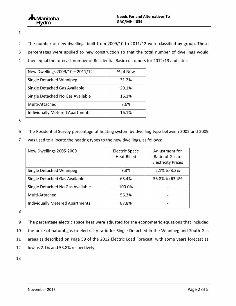
Needs For and Alternatives To GAC/MH I-034
1
The number of new dwellings built from 2009/10 to 2011/12 were classified by group. These 2
percentages were applied to new construction so that the total number of dwellings would 3
then equal the forecast number of Residential Basic customers for 2012/13 and later. 4
New Dwellings 2009/10 – 2011/12 % of New
Single Detached Winnipeg 31.2%
Single Detached Gas Available 29.1%
Single Detached No Gas Available 16.1%
Multi-Attached 7.6%
Individually Metered Apartments 16.1%
5
The Residential Survey percentage of heating system by dwelling type between 2005 and 2009 6
was used to allocate the heating types to the new dwellings, as follows: 7
New Dwellings 2005-2009 Electric Space Heat Billed
Adjustment for Ratio of Gas to
Electricity Prices
Single Detached Winnipeg 3.3% 2.1% to 3.3%
Single Detached Gas Available 63.4% 53.8% to 63.4%
Single Detached No Gas Available 100.0% -
Multi-Attached 56.3% -
Individually Metered Apartments 87.8% -
8
The percentage electric space heat were adjusted for the econometric equations that included 9
the price of natural gas to electricity ratio for Single Detached in the Winnipeg and South Gas 10
areas as described on Page 59 of the 2012 Electric Load Forecast, with some years forecast as 11
low as 2.1% and 53.8% respectively. 12
13
November 2013 Page 2 of 5

Needs For and Alternatives To GAC/MH I-034
This information was assembled to forecast each of the five areas and dwelling types for both 1
electric heat billed and other heat. The following two tables provide the detailed number of 2
customers that formed the basis of the electric space heat saturation rate. 3
Electric Space Heat Billed (average annual customers) SD Winnipeg SD Gas Avail SD No Gas Avail Multi-Attached Apartments Total
2011/12 6,625 53,138 71,075 9,046 21,195 161,078 2012/13 6,875 54,062 71,908 9,361 21,960 164,166 2013/14 7,119 55,120 72,938 9,677 22,811 167,665 2014/15 7,367 56,248 74,024 10,006 23,713 171,358 2015/16 7,618 57,413 75,121 10,336 24,624 175,111 2016/17 7,869 58,599 76,225 10,665 25,544 178,901 2017/18 8,117 59,798 77,335 10,994 26,469 182,714 2018/19 8,362 61,001 78,450 11,322 27,400 186,536 2019/20 8,602 62,204 79,567 11,650 28,334 190,355 2020/21 8,836 63,402 80,684 11,975 29,268 194,165 2021/22 9,064 64,591 81,799 12,299 30,202 197,955 2022/23 9,286 65,772 82,910 12,620 31,134 201,721 2023/24 9,502 66,942 84,015 12,938 32,061 205,458 2024/25 9,711 68,101 85,113 13,254 32,983 209,162 2025/26 9,916 69,254 86,203 13,566 33,898 212,837 2026/27 10,117 70,405 87,284 13,874 34,807 216,488 2027/28 10,313 71,554 88,356 14,180 35,709 220,113 2028/29 10,506 72,701 89,419 14,482 36,603 223,712 2029/30 10,696 73,845 90,473 14,780 37,491 227,286 2030/31 10,882 74,988 91,518 15,076 38,372 230,835 2031/32 11,065 76,129 92,555 15,369 39,246 234,364
4
5
November 2013 Page 3 of 5

Needs For and Alternatives To GAC/MH I-034
1
Other Heat (average annual customers)
SD Winnipeg
SD Gas Avail
SD No Gas Avail
Multi-Attached
Apartments 2nd meter
Total
2011/12 159,327 59,913 7,090 24,992 36,120 2,227 289,670 2012/13 161,014 60,442 7,013 25,120 36,215 2,310 292,114 2013/14 162,620 61,111 6,937 25,254 36,321 2,310 294,552 2014/15 164,335 61,814 6,862 25,402 36,433 2,310 297,157 2015/16 166,067 62,500 6,787 25,555 36,547 2,310 299,766 2016/17 167,816 63,180 6,713 25,712 36,661 2,310 302,391 2017/18 169,580 63,859 6,640 25,872 36,776 2,310 305,037 2018/19 171,357 64,543 6,567 26,036 36,891 2,310 307,703 2019/20 173,145 65,233 6,495 26,202 37,005 2,310 310,390 2020/21 174,940 65,929 6,424 26,369 37,120 2,310 313,092 2021/22 176,739 66,631 6,353 26,539 37,234 2,310 315,805 2022/23 178,537 67,336 6,283 26,709 37,347 2,310 318,521 2023/24 180,332 68,041 6,213 26,879 37,459 2,310 321,234 2024/25 182,120 68,746 6,144 27,050 37,570 2,310 323,939 2025/26 183,898 69,443 6,076 27,220 37,679 2,310 326,626 2026/27 185,664 70,128 6,008 27,389 37,787 2,310 329,286 2027/28 187,418 70,799 5,941 27,558 37,894 2,310 331,920 2028/29 189,159 71,458 5,875 27,727 37,999 2,310 334,526 2029/30 190,886 72,103 5,809 27,894 38,102 2,310 337,105 2030/31 192,602 72,735 5,744 28,061 38,205 2,310 339,656 2031/32 194,306 73,355 5,679 28,227 38,306 2,310 342,181
1.0% 1.0% -1.1% 0.6% 0.3% 0.2% 0.8% 2
The “2nd meter” are dwellings that have more than one Residential Basic meter. 3
4
The following table shows the breakdown of electric heat percentage by area and dwelling type 5
by dividing the Electric Space Heat customers for each customers category by all customers 6
within each customer category (the sum of the Electric Space Heat customers and the Other 7
Heat customers). The final column labeled “Total” was used as the “% Elec Space Heat” column 8
in Table 14 on page 18 of the 2012 Electric Load Forecast included as Appendix C of this 9
submission. 10
November 2013 Page 4 of 5

Needs For and Alternatives To GAC/MH I-034
% Electric Space Heat Billed SD
Winnipeg SD Gas Avail
SD No Gas Avail
Multi-Attached
Apartments 2nd meter
Total
2011/12 4.0% 47.0% 90.9% 26.6% 37.0% 0.0% 35.7% 2012/13 4.1% 47.2% 91.1% 27.1% 37.7% 0.0% 36.0% 2013/14 4.2% 47.4% 91.3% 27.7% 38.6% 0.0% 36.3% 2014/15 4.3% 47.6% 91.5% 28.3% 39.4% 0.0% 36.6% 2015/16 4.4% 47.9% 91.7% 28.8% 40.3% 0.0% 36.9% 2016/17 4.5% 48.1% 91.9% 29.3% 41.1% 0.0% 37.2% 2017/18 4.6% 48.4% 92.1% 29.8% 41.9% 0.0% 37.5% 2018/19 4.7% 48.6% 92.3% 30.3% 42.6% 0.0% 37.7% 2019/20 4.7% 48.8% 92.5% 30.8% 43.4% 0.0% 38.0% 2020/21 4.8% 49.0% 92.6% 31.2% 44.1% 0.0% 38.3% 2021/22 4.9% 49.2% 92.8% 31.7% 44.8% 0.0% 38.5% 2022/23 4.9% 49.4% 93.0% 32.1% 45.5% 0.0% 38.8% 2023/24 5.0% 49.6% 93.1% 32.5% 46.1% 0.0% 39.0% 2024/25 5.1% 49.8% 93.3% 32.9% 46.7% 0.0% 39.2% 2025/26 5.1% 49.9% 93.4% 33.3% 47.4% 0.0% 39.5% 2026/27 5.2% 50.1% 93.6% 33.6% 47.9% 0.0% 39.7% 2027/28 5.2% 50.3% 93.7% 34.0% 48.5% 0.0% 39.9% 2028/29 5.3% 50.4% 93.8% 34.3% 49.1% 0.0% 40.1% 2029/30 5.3% 50.6% 94.0% 34.6% 49.6% 0.0% 40.3% 2030/31 5.3% 50.8% 94.1% 34.9% 50.1% 0.0% 40.5% 2031/32 5.4% 50.9% 94.2% 35.3% 50.6% 0.0% 40.6%
1
November 2013 Page 5 of 5

Needs For and Alternatives To GAC/MH I-035
REFERENCE: Chapter 4: The Need for New Resources 1
2
QUESTION: 3
For each year of the forecast, please provide the residential annual MWh and MW assuming no 4
increase in the saturation rate of electric space heating. 5
6
RESPONSE: 7
In Order 119/13 the PUB determined that it did not require this Information Request to be 8
answered at this time. 9
November 2013 Page 1 of 1

Needs For and Alternatives To GAC/MH I‐036
November 2013 Page 1 of 2
REFERENCE: Chapter 4: The Need for New Resources 1
2
QUESTION: 3
For each year of the forecast, please provide the number of new customers in gas available 4
areas, broken out by space heating source. 5
6
RESPONSE: 7
For each year of the 2012 forecast, the following table shows the numbers of new single 8
detached dwellings in Gas Available areas, broken out by space heating fuel source. 9
10
Forecast Year
Electric Heat
Winnipeg
Other Heat
Winnipeg
Electric Heat
Gas Area
Other Heat
Gas Area
Electric Heat Total
Other Heat Total
2012/13 44 1,820 923 785 967 2,605
2013/14 46 2,032 1,016 892 1,062 2,924
2014/15 53 2,048 1,062 867 1,115 2,915
2015/16 56 2,066 1,087 861 1,143 2,927
2016/17 57 2,081 1,102 862 1,159 2,943
2017/18 57 2,094 1,110 865 1,167 2,959
2018/19 56 2,104 1,110 874 1,166 2,978
2019/20 54 2,111 1,106 883 1,160 2,994
2020/21 52 2,114 1,098 892 1,150 3,006
2021/22 50 2,113 1,088 899 1,138 3,012
2022/23 48 2,108 1,078 902 1,126 3,010
2023/24 46 2,100 1,067 904 1,113 3,004
2024/25 44 2,090 1,055 904 1,099 2,994
2025/26 45 2,075 1,053 894 1,098 2,969
2026/27 45 2,060 1,050 883 1,095 2,943
2027/28 45 2,045 1,048 871 1,093 2,916

Needs For and Alternatives To GAC/MH I‐036
November 2013 Page 2 of 2
2028/29 45 2,030 1,045 860 1,090 2,890
2029/30 46 2,014 1,042 848 1,088 2,862
2030/31 46 2,000 1,040 837 1,086 2,837
2031/32 46 1,988 1,039 827 1,085 2,815

Needs For and Alternatives To GAC/MH I‐037
November 2013 Page 1 of 2
REFERENCE: Chapter 4: The Need for New Resources 1
2
QUESTION: 3
For each year of the forecast, please provide the number of new customers in areas not served 4
by gas, broken out by space heating source. 5
6
RESPONSE: 7
For each year of the 2012 forecast, the following table shows the numbers of new single 8
detached dwellings in No Gas Available areas, broken out by space heating fuel source. 9
10
Forecast Year
Electric Heat Total
Other Heat Total
2012/13 955 0
2013/14 1,065 0
2014/15 1,077 0
2015/16 1,087 0
2016/17 1,096 0
2017/18 1,102 0
2018/19 1,107 0
2019/20 1,110 0
2020/21 1,111 0
2021/22 1,109 0
2022/23 1,105 0
2023/24 1,100 0
2024/25 1,094 0
2025/26 1,087 0
2026/27 1,079 0
2027/28 1,071 0

Needs For and Alternatives To GAC/MH I‐037
November 2013 Page 2 of 2
2028/29 1,063 0
2029/30 1,056 0
2030/31 1,048 0
2031/32 1,042 0

Needs For and Alternatives To GAC/MH I‐038
November 2013 Page 1 of 2
REFERENCE: Chapter 4: The Need for New Resources 1
2
QUESTION: 3
For each year of the forecast, please provide the number space heating retrofits in gas available 4
areas, broken out by space heating source. 5
6
RESPONSE: 7
For each year of the 2012 forecast, the following table shows the numbers of annual retrofit 8
space heating systems in single detached dwellings in Gas Available areas, broken out by space 9
heating source. 10
11
Forecast Year
Electric Heat
Winnipeg
Other Heat
Winnipeg
Electric Heat
Gas Area
Other Heat
Gas Area
Electric Heat Total
Other Heat Total
2012/13 466 9,590 2,001 3,387 2,467 12,977
2013/14 473 9,744 2,037 3,445 2,510 13,189
2014/15 480 9,893 2,077 3,503 2,557 13,396
2015/16 487 10,026 2,118 3,554 2,605 13,580
2016/17 492 10,145 2,161 3,598 2,653 13,743
2017/18 497 10,250 2,204 3,638 2,701 13,888
2018/19 502 10,342 2,247 3,672 2,749 14,014
2019/20 506 10,421 2,290 3,703 2,796 14,124
2020/21 509 10,490 2,333 3,729 2,842 14,219
2021/22 512 10,548 2,375 3,753 2,887 14,301
2022/23 514 10,598 2,417 3,774 2,931 14,372
2023/24 516 10,640 2,458 3,792 2,974 14,432
2024/25 518 10,676 2,498 3,808 3,016 14,484
2025/26 519 10,707 2,538 3,823 3,057 14,530
2026/27 521 10,735 2,577 3,836 3,098 14,571

Needs For and Alternatives To GAC/MH I‐038
November 2013 Page 2 of 2
2027/28 522 10,760 2,617 3,847 3,139 14,607
2028/29 523 10,784 2,656 3,858 3,179 14,642
2029/30 524 10,809 2,695 3,868 3,219 14,677
2030/31 525 10,835 2,734 3,879 3,259 14,714
2031/32 527 10,863 2,774 3,889 3,301 14,752
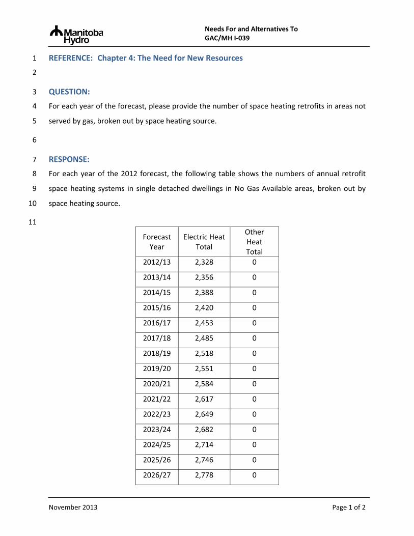
Needs For and Alternatives To GAC/MH I‐039
November 2013 Page 1 of 2
REFERENCE: Chapter 4: The Need for New Resources 1
2
QUESTION: 3
For each year of the forecast, please provide the number of space heating retrofits in areas not 4
served by gas, broken out by space heating source. 5
6
RESPONSE: 7
For each year of the 2012 forecast, the following table shows the numbers of annual retrofit 8
space heating systems in single detached dwellings in No Gas Available areas, broken out by 9
space heating source. 10
11
Forecast Year
Electric Heat Total
Other Heat Total
2012/13 2,328 0
2013/14 2,356 0
2014/15 2,388 0
2015/16 2,420 0
2016/17 2,453 0
2017/18 2,485 0
2018/19 2,518 0
2019/20 2,551 0
2020/21 2,584 0
2021/22 2,617 0
2022/23 2,649 0
2023/24 2,682 0
2024/25 2,714 0
2025/26 2,746 0
2026/27 2,778 0
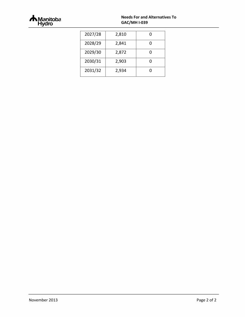
Needs For and Alternatives To GAC/MH I‐039
November 2013 Page 2 of 2
2027/28 2,810 0
2028/29 2,841 0
2029/30 2,872 0
2030/31 2,903 0
2031/32 2,934 0

Needs For and Alternatives To GAC/MH I‐040
November 2013 Page 1 of 1
REFERENCE: Chapter 4: The Need for New Resources 1
2
QUESTION: 3
For each year of the forecast, please provide the average annual electricity use of heating and 4
non‐heating residential customers. 5
6
RESPONSE: 7
The average annual electricity use of heating and non‐heating residential customers is provided 8
on page 18 of the 2012 Electric Load Forecast included as Appendix C of the submission. 9

Needs For and Alternatives To GAC/MH I-041
REFERENCE: Chapter 4: The Need for New Resources; Section: 4.2.1.2; Page No.: 12 1
2
PREAMBLE: Manitoba Hydro projects in its 2012 forecast that the saturation rate of 3 residential electric water heating will grow from 47% currently to 69% by 2031/32. 4
5
QUESTION: 6
Please provide the basis for the projection of a 69% electric water heating saturation rate, 7
including all data, assumptions, calculations and spreadsheets (with formulas intact) 8
9
RESPONSE: 10
The 69% electric water heat projection referred to in NFAT chapter 4 was a reference to the “% 11
Elec Water Tanks” column in Table 14 on page 18 of the 2012 Electric Load Forecast included as 12
Appendix C of this submission. The electric water heating saturations shown in this table start 13
at 47.3% in 2011/12 and grow to 69.1% in 2031/32. 14
15
Residential survey data was used to provide the starting number of water heating tanks in 16
2009/10 broken down by Single Detached, Multi-Attached and Apartments. The Single-17
Detached were further broken down by Winnipeg, Gas Available (excluding Winnipeg) and No 18
Gas Available areas. For each of the five groups, the survey provided the starting number of 19
private electric water heaters and other water heaters. 20
21
The number of new water heaters were forecast each year. This was made up of water heaters 22
in new homes, and water heaters being replaced in existing homes. An average lifetime of 12 23
years was used for a water heater. Based on data from the 2009 Residential survey, 30.3% of 24
natural gas water heaters were found to be replaced with electric water heaters. 100% of 25
electric water heaters were found to be replaced with electric water heaters. These 26
replacement rates were used for replacement water tanks. In newly constructed homes, 100% 27
November 2013 Page 1 of 4

Needs For and Alternatives To GAC/MH I-041
of water heaters were assumed to be electric based upon saturation rates for homes 1
constructed from 2005 to 2009 reported under the 2009 Residential survey. 2
3
This information was assembled to forecast each of the five areas and dwelling types for both 4
private electric water heaters and other water heaters. The following two tables provide the 5
detailed number of water heaters that formed the basis of the electric water heat saturation 6
rate. 7
8
Private Electric Water Heaters (average annual customers)
SD Winnipeg SD Gas Avail SD No Gas Avail Multi-Attached Apartments Total
2011/12 45,517 72,318 76,029 11,764 7,478 213,106 2012/13 50,232 74,634 76,803 12,505 7,753 221,927 2013/14 55,588 77,448 77,753 13,348 8,061 232,199 2014/15 60,757 80,265 78,761 14,173 8,384 242,340 2015/16 65,838 83,067 79,783 14,990 8,710 252,387 2016/17 70,844 85,853 80,811 15,797 9,037 262,342 2017/18 75,645 88,579 81,846 16,579 9,366 272,015 2018/19 80,319 91,269 82,888 17,345 9,696 281,518 2019/20 84,884 93,926 83,932 18,098 10,026 290,866 2020/21 89,315 96,541 84,977 18,835 10,355 300,023 2021/22 93,635 99,117 86,021 19,559 10,684 309,017 2022/23 97,881 101,666 87,063 20,275 11,011 317,897 2023/24 103,476 104,685 88,125 21,181 11,343 328,809 2024/25 109,513 107,814 89,139 22,141 11,673 340,279 2025/26 114,279 110,515 90,153 22,930 11,996 349,874 2026/27 118,396 112,992 91,164 23,633 12,316 358,502 2027/28 122,214 115,362 92,169 24,298 12,634 366,676 2028/29 125,913 117,681 93,167 24,947 12,948 374,656 2029/30 129,552 119,967 94,156 25,588 13,260 382,522 2030/31 133,167 122,276 95,138 26,228 13,570 390,380 2031/32 136,790 124,622 96,112 26,870 13,878 398,273
9
November 2013 Page 2 of 4
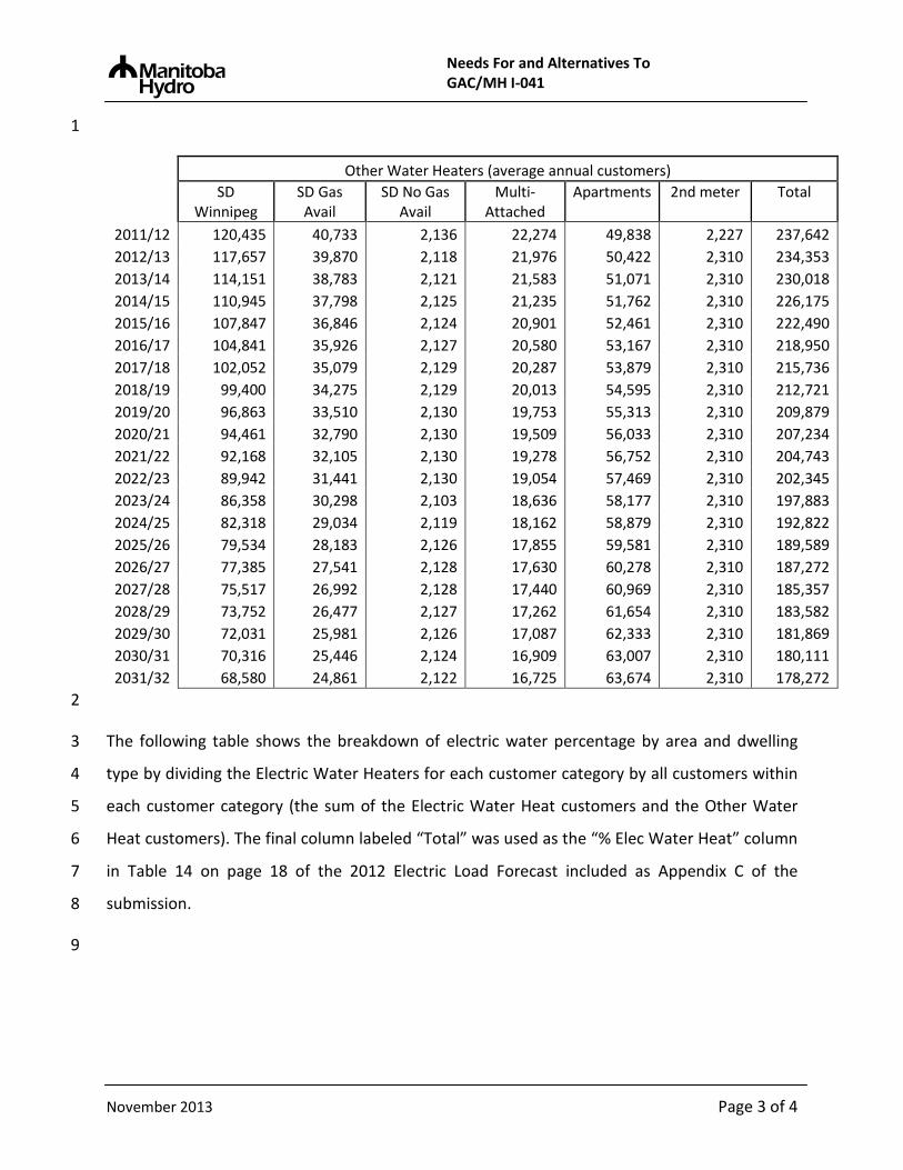
Needs For and Alternatives To GAC/MH I-041
1
Other Water Heaters (average annual customers)
SD Winnipeg
SD Gas Avail
SD No Gas Avail
Multi-Attached
Apartments 2nd meter Total
2011/12 120,435 40,733 2,136 22,274 49,838 2,227 237,642 2012/13 117,657 39,870 2,118 21,976 50,422 2,310 234,353 2013/14 114,151 38,783 2,121 21,583 51,071 2,310 230,018 2014/15 110,945 37,798 2,125 21,235 51,762 2,310 226,175 2015/16 107,847 36,846 2,124 20,901 52,461 2,310 222,490 2016/17 104,841 35,926 2,127 20,580 53,167 2,310 218,950 2017/18 102,052 35,079 2,129 20,287 53,879 2,310 215,736 2018/19 99,400 34,275 2,129 20,013 54,595 2,310 212,721 2019/20 96,863 33,510 2,130 19,753 55,313 2,310 209,879 2020/21 94,461 32,790 2,130 19,509 56,033 2,310 207,234 2021/22 92,168 32,105 2,130 19,278 56,752 2,310 204,743 2022/23 89,942 31,441 2,130 19,054 57,469 2,310 202,345 2023/24 86,358 30,298 2,103 18,636 58,177 2,310 197,883 2024/25 82,318 29,034 2,119 18,162 58,879 2,310 192,822 2025/26 79,534 28,183 2,126 17,855 59,581 2,310 189,589 2026/27 77,385 27,541 2,128 17,630 60,278 2,310 187,272 2027/28 75,517 26,992 2,128 17,440 60,969 2,310 185,357 2028/29 73,752 26,477 2,127 17,262 61,654 2,310 183,582 2029/30 72,031 25,981 2,126 17,087 62,333 2,310 181,869 2030/31 70,316 25,446 2,124 16,909 63,007 2,310 180,111 2031/32 68,580 24,861 2,122 16,725 63,674 2,310 178,272
2
The following table shows the breakdown of electric water percentage by area and dwelling 3
type by dividing the Electric Water Heaters for each customer category by all customers within 4
each customer category (the sum of the Electric Water Heat customers and the Other Water 5
Heat customers). The final column labeled “Total” was used as the “% Elec Water Heat” column 6
in Table 14 on page 18 of the 2012 Electric Load Forecast included as Appendix C of the 7
submission. 8
9
November 2013 Page 3 of 4

Needs For and Alternatives To GAC/MH I-041
1
% Private Electric Water Heaters
SD Winnipeg
SD Gas Avail
SD No Gas Avail
Multi-Attached
Apartments Total
2011/12 27.4% 64.0% 97.3% 34.6% 13.0% 47.3% 2012/13 29.9% 65.2% 97.3% 36.3% 13.3% 48.6% 2013/14 32.7% 66.6% 97.3% 38.2% 13.6% 50.2% 2014/15 35.4% 68.0% 97.4% 40.0% 13.9% 51.7% 2015/16 37.9% 69.3% 97.4% 41.8% 14.2% 53.1% 2016/17 40.3% 70.5% 97.4% 43.4% 14.5% 54.5% 2017/18 42.6% 71.6% 97.5% 45.0% 14.8% 55.8% 2018/19 44.7% 72.7% 97.5% 46.4% 15.1% 57.0% 2019/20 46.7% 73.7% 97.5% 47.8% 15.3% 58.1% 2020/21 48.6% 74.6% 97.6% 49.1% 15.6% 59.1% 2021/22 50.4% 75.5% 97.6% 50.4% 15.8% 60.1% 2022/23 52.1% 76.4% 97.6% 51.6% 16.1% 61.1% 2023/24 54.5% 77.6% 97.7% 53.2% 16.3% 62.4% 2024/25 57.1% 78.8% 97.7% 54.9% 16.5% 63.8% 2025/26 59.0% 79.7% 97.7% 56.2% 16.8% 64.9% 2026/27 60.5% 80.4% 97.7% 57.3% 17.0% 65.7% 2027/28 61.8% 81.0% 97.7% 58.2% 17.2% 66.4% 2028/29 63.1% 81.6% 97.8% 59.1% 17.4% 67.1% 2029/30 64.3% 82.2% 97.8% 60.0% 17.5% 67.8% 2030/31 65.4% 82.8% 97.8% 60.8% 17.7% 68.4% 2031/32 66.6% 83.4% 97.8% 61.6% 17.9% 69.1%
2
November 2013 Page 4 of 4

Needs For and Alternatives To GAC/MH I-042
REFERENCE: Chapter 4: The Need for New Resources; 1
2
QUESTION: 3
For each year of the forecast, please provide the basic residential MWh and MW assuming no 4
increase in the saturation rate of electric water heating. 5
6
RESPONSE: 7
In Order 119/13 the PUB determined that it did not require this Information Request to be 8
answered at this time. 9
November 2013 Page 1 of 1

Needs For and Alternatives To GAC/MH I‐043
November 2013 Page 1 of 2
REFERENCE: Chapter 4: The Need for New Resources 1
2
QUESTION: 3
For each year of the forecast, please provide the number of new customers in gas available 4
areas, broken out by water heating source. 5
6
RESPONSE: 7
For each year of the 2012 forecast, the following table shows the numbers of new single 8
detached dwellings in Gas Available areas, broken out by water heating fuel source. 9
10
Forecast Year
Electric Water
Winnipeg
Other Water
Winnipeg
Electric Water
Gas Area
Other Water
Gas Area
Electric Water Total
Other Water Total
2012/13 1,864 0 1,708 0 3,572 0
2013/14 2,078 0 1,908 0 3,986 0
2014/15 2,101 0 1,929 0 4,030 0
2015/16 2,121 0 1,948 0 4,069 0
2016/17 2,137 0 1,963 0 4,100 0
2017/18 2,151 0 1,975 0 4,126 0
2018/19 2,160 0 1,984 0 4,144 0
2019/20 2,165 0 1,989 0 4,154 0
2020/21 2,166 0 1,990 0 4,156 0
2021/22 2,163 0 1,987 0 4,150 0
2022/23 2,156 0 1,981 0 4,137 0
2023/24 2,146 0 1,971 0 4,117 0
2024/25 2,134 0 1,960 0 4,094 0
2025/26 2,120 0 1,947 0 4,067 0
2026/27 2,105 0 1,933 0 4,038 0
2027/28 2,090 0 1,919 0 4,009 0

Needs For and Alternatives To GAC/MH I‐043
November 2013 Page 2 of 2
2028/29 2,075 0 1,905 0 3,980 0
2029/30 2,060 0 1,891 0 3,951 0
2030/31 2,046 0 1,878 0 3,924 0
2031/32 2,034 0 1,867 0 3,901 0

Needs For and Alternatives To GAC/MH I‐044
November 2013 Page 1 of 2
REFERENCE: Chapter 4: The Need for New Resources 1
2
QUESTION: 3
For each year of the forecast, please provide the number of new customers in areas not served 4
by gas, broken out by water heating source. 5
6
RESPONSE: 7
For each year of the 2012 forecast, the following table shows the numbers of New single 8
detached dwellings in No Gas Available areas, broken out by water heating source. 9
10
Forecast Year
Electric Water Total
Other Water Total
2012/13 955 0
2013/14 1,065 0
2014/15 1,077 0
2015/16 1,087 0
2016/17 1,096 0
2017/18 1,102 0
2018/19 1,107 0
2019/20 1,110 0
2020/21 1,111 0
2021/22 1,109 0
2022/23 1,105 0
2023/24 1,100 0
2024/25 1,094 0
2025/26 1,087 0
2026/27 1,079 0
2027/28 1,071 0
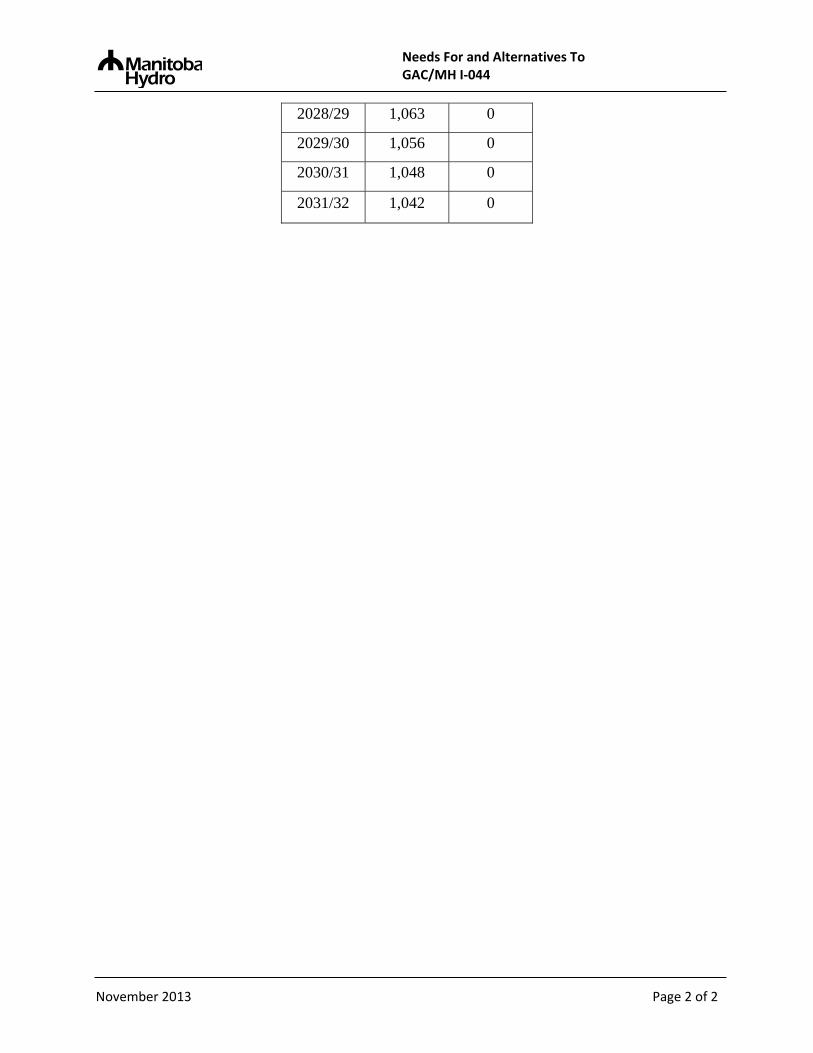
Needs For and Alternatives To GAC/MH I‐044
November 2013 Page 2 of 2
2028/29 1,063 0
2029/30 1,056 0
2030/31 1,048 0
2031/32 1,042 0

Needs For and Alternatives To GAC/MH I‐045
November 2013 Page 1 of 2
REFERENCE: Chapter 4: The Need for New Resources 1
2
QUESTION: 3
For each year of the forecast, please provide the number water heating retrofits in gas available 4
areas, broken out by water heating source. 5
6
RESPONSE: 7
For each year of the 2012 forecast, the following table shows the number of water heating 8
retrofits in single detached dwellings in Gas Available areas, broken out by water heating fuel 9
source. 10
11
Forecast Year
Electric Water
Winnipeg
Other Water
Winnipeg
Electric Water
Gas Area
Other Water
Gas Area
Electric Water Total
Other Water Total
2012/13 3,707 9,847 5,748 3,288 9,455 13,135
2013/14 4,128 9,546 5,967 3,189 10,095 12,735
2014/15 4,537 9,274 6,193 3,099 10,730 12,373
2015/16 4,923 9,030 6,414 3,016 11,337 12,046
2016/17 5,310 8,785 6,637 2,932 11,947 11,717
2017/18 5,674 8,565 6,855 2,854 12,529 11,419
2018/19 6,018 8,368 7,069 2,782 13,087 11,150
2019/20 6,353 8,182 7,281 2,712 13,634 10,894
2020/21 6,669 8,015 7,490 2,646 14,159 10,661
2021/22 6,970 7,864 7,696 2,583 14,666 10,447
2022/23 7,258 7,727 7,899 2,523 15,157 10,250
2023/24 7,534 7,602 8,100 2,464 15,634 10,066
2024/25 8,014 7,260 8,372 2,329 16,386 9,589
2025/26 8,354 7,064 8,598 2,242 16,952 9,306
2026/27 8,623 6,944 8,801 2,178 17,424 9,122
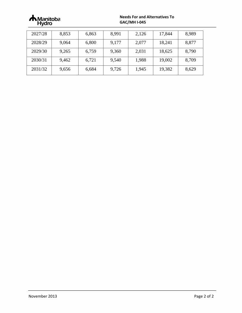
Needs For and Alternatives To GAC/MH I‐045
November 2013 Page 2 of 2
2027/28 8,853 6,863 8,991 2,126 17,844 8,989
2028/29 9,064 6,800 9,177 2,077 18,241 8,877
2029/30 9,265 6,759 9,360 2,031 18,625 8,790
2030/31 9,462 6,721 9,540 1,988 19,002 8,709
2031/32 9,656 6,684 9,726 1,945 19,382 8,629

Needs For and Alternatives To GAC/MH I‐046
November 2013 Page 1 of 2
REFERENCE: Chapter 4: The Need for New Resources 1
2
QUESTION: 3
For each year of the forecast, please provide the number of water heating retrofits in areas not 4
served by gas, broken out by space heating source. 5
6
RESPONSE: 7
For each year of the 2012 forecast, the following table shows the number of water heating 8
retrofits in single detached dwellings in Gas Unavailable areas, broken out by water heating fuel 9
source. 10
11
Forecast Year
Electric Water Total
Other Water Total
2012/13 5,967 157
2013/14 6,038 157
2014/15 6,116 157
2015/16 6,196 156
2016/17 6,276 156
2017/18 6,357 156
2018/19 6,438 156
2019/20 6,520 156
2020/21 6,602 156
2021/22 6,684 156
2022/23 6,765 156
2023/24 6,847 156
2024/25 6,928 155
2025/26 7,008 155
2026/27 7,087 155

Needs For and Alternatives To GAC/MH I‐046
November 2013 Page 2 of 2
2027/28 7,167 155
2028/29 7,245 155
2029/30 7,323 155
2030/31 7,400 155
2031/32 7,476 155

Needs For and Alternatives To GAC/MH I‐047
November 2013 Page 1 of 1
REFERENCE: Chapter 4: The Need for New Resources 1
2
QUESTION: 3
For each year of the forecast, provide the number of water heater retrofits where gas is 4
replaced with electric equipment. 5
6
RESPONSE: 7
The number of water heater retrofits where natural gas is replaced with electric equipment was 8
not specifically calculated or modeled under the 2012 forecast. 9

Needs For and Alternatives To GAC/MH I‐048
November 2013 Page 1 of 1
REFERENCE: Appendix D 2013 Electric Load Forecast; Page No.: 54 1
2
PREAMBLE: MH projects in its 2013 forecast that the saturation rate of electric space 3
heating will grow from 35% currently to 39.3% by 2032/33. 4
5
QUESTION: 6
Please provide the number of existing residential customers in areas where gas is unavailable, 7
broken out by space heating source. 8
9
RESPONSE: 10
For the 2013 forecast, the number of residential existing single detached dwellings in No Gas 11
Available areas broken out by space heating fuel source is as follows: 12
13
Space Heating Source Existing Single Detached
Electric Heat Billed 73,024
Other Space Heat Source 6,212
Total No Gas Available Area 79,236
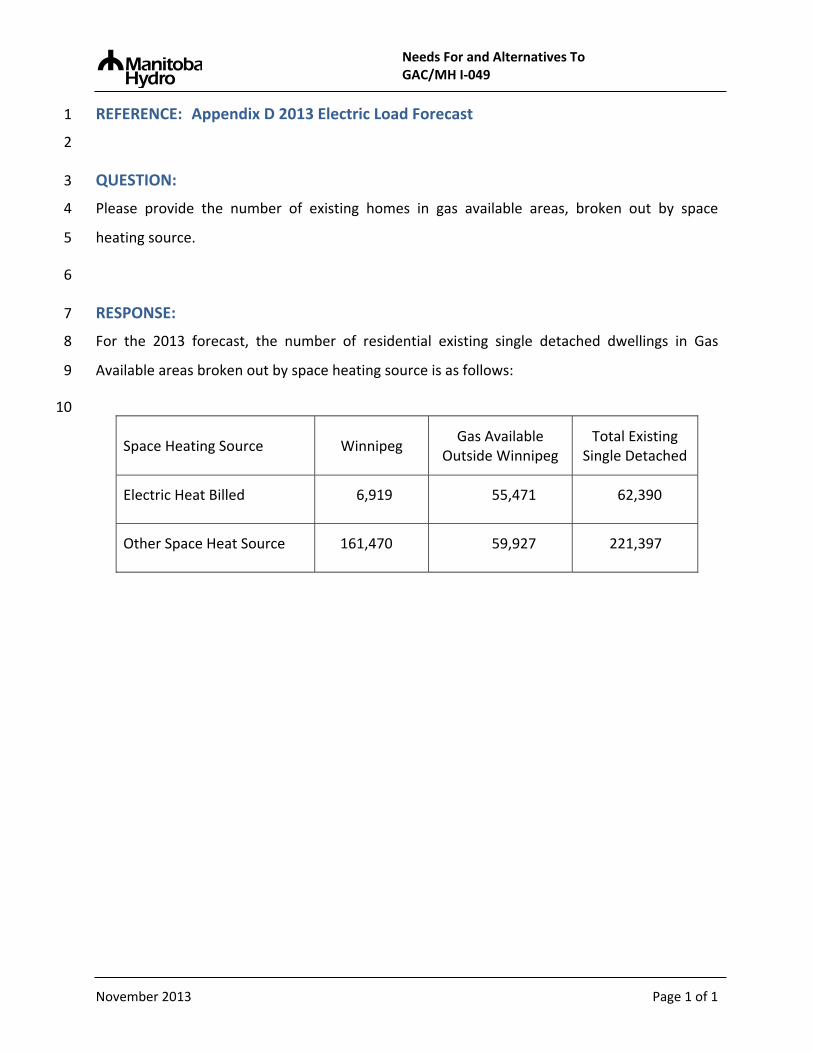
Needs For and Alternatives To GAC/MH I‐049
November 2013 Page 1 of 1
REFERENCE: Appendix D 2013 Electric Load Forecast 1
2
QUESTION: 3
Please provide the number of existing homes in gas available areas, broken out by space 4
heating source. 5
6
RESPONSE: 7
For the 2013 forecast, the number of residential existing single detached dwellings in Gas 8
Available areas broken out by space heating source is as follows: 9
10
Space Heating Source
Winnipeg
Gas Available Outside Winnipeg
Total Existing Single Detached
Electric Heat Billed 6,919 55,471 62,390
Other Space Heat Source 161,470 59,927 221,397

Needs For and Alternatives To GAC/MH I‐050
November 2013 Page 1 of 1
REFERENCE: Appendix D 2013 Electric Load Forecast 1
2
QUESTION: 3
Please provide the number of existing residential customers in areas where gas is unavailable, 4
broken out by water heating source. 5
6
RESPONSE: 7
For the 2013 forecast, the number of residential existing single detached dwellings in No Gas 8
Available areas broken out by water heating fuel sources is as follows: 9
10
Water Heating Source Existing Single Detached
Electric Water Heat Billed 77,231
Other Water Heat Source 2,005
Total No Gas Available Area 79,236
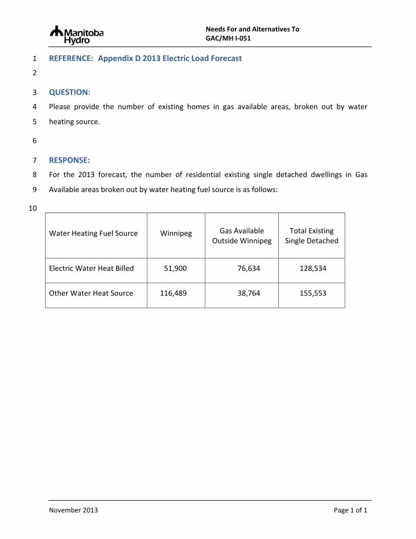
Needs For and Alternatives To GAC/MH I‐051
November 2013 Page 1 of 1
REFERENCE: Appendix D 2013 Electric Load Forecast 1
2
QUESTION: 3
Please provide the number of existing homes in gas available areas, broken out by water 4
heating source. 5
6
RESPONSE: 7
For the 2013 forecast, the number of residential existing single detached dwellings in Gas 8
Available areas broken out by water heating fuel source is as follows: 9
10
Water Heating Fuel Source
Winnipeg
Gas Available Outside Winnipeg
Total Existing Single Detached
Electric Water Heat Billed 51,900 76,634 128,534
Other Water Heat Source 116,489 38,764 155,553

Needs For and Alternatives To GAC/MH I-052
REFERENCE: Appendix D 2013 Electric Load Forecast 1
2
QUESTION: 3
Please provide the basis for the projection of a 39.3% electric space heating saturation rate, 4
including all data, assumptions, calculations and spreadsheets (with formulas intact) 5
6
RESPONSE: 7
The 39.3% electric space heat projection is the forecast for the saturation of electric heat in 8
2032/33, as shown in the “% Elec Space Heat” column in Table 14 on page 18 of the 2013 9
Electric Load Forecast included as Appendix D of this submission. 10
11
The general approach for determining the electric space heat saturation is described in the 12
Residential Basic Methodology section of the 2013 Electric Load Forecast starting on page 59. 13
The steps are similar to those used in the 2012 Electric Load Forecast as outlined in Manitoba 14
Hydro’s response to GAC/MH I-034. Differences from the procedure outlined for the 2012 15
Forecast will be presented in this response. 16
17
The “Total Basic Custs” column is as forecasted in Manitoba Hydro’s 2013 Economic Outlook 18
included as Appendix G of the submission. 19
20
Five years of data, from 2008/09 to 2012/13 were used to classify the number of new dwellings 21
built, as follows: 22
New Dwellings 2008/09 – 2012/13 % of New
Single Detached Winnipeg 27.5%
Single Detached Gas Available 30.5%
Single Detached No Gas Available 16.6%
November 2013 Page 1 of 4

Needs For and Alternatives To GAC/MH I-052
Multi-Attached 7.3%
Individually Metered Apartments 18.2%
1
The Residential Survey percentage of heating system by dwelling type between 2005 and 2009 2
was used to allocate the heating types to the new dwellings. However, the additional 2012/13 3
year of data indicated that the effect of the ratio of gas to electricity prices was no longer 4
significant, and the percentages were used without adjustment: 5
New Dwellings 2005-2009 Electric Space Heat Billed
Adjustment for Ratio of Gas to
Electricity Prices
Single Detached Winnipeg 3.3% -
Single Detached Gas Available 63.4% -
Single Detached No Gas Available 100.0% -
Multi-Attached 56.3% -
Individually Metered Apartments 87.8% -
6
The forecast numbers of customers by heating fuel were then adjusted to reflect the forecast 7
impact of Manitoba Hydro’s heating fuel choice initiative as detailed in Manitoba Hydro’s 8
response to PUB/MH I-0253 (a). 9
10
The following two tables provide the detailed number of customers that formed the basis of 11
the electric space heat saturation rate in the 2013 forecast. They include the expected effects 12
of Manitoba Hydro’s heating fuel choice initiative. 13
Electric Space Heat Billed (average annual customers)
SD Winnipeg SD Gas Avail SD No Gas Avail Multi-Attached Apartments Total 2012/13 6,811 54,817 72,512 9,320 22,115 165,576 2013/14 6,999 56,099 73,650 9,595 23,105 169,399 2014/15 7,150 57,283 74,841 9,858 23,997 173,080 2015/16 7,278 58,414 76,018 10,113 24,890 176,666 2016/17 7,364 59,458 77,183 10,357 25,781 180,099
November 2013 Page 2 of 4

Needs For and Alternatives To GAC/MH I-052
2017/18 7,424 60,398 78,341 10,583 26,677 183,380 2018/19 7,475 61,211 79,496 10,781 27,579 186,502 2019/20 7,519 61,912 80,646 10,954 28,486 189,479 2020/21 7,557 62,539 81,788 11,112 29,396 192,355 2021/22 7,589 63,106 82,920 11,256 30,306 195,141 2022/23 7,614 63,595 84,041 11,383 31,213 197,812 2023/24 7,633 64,037 85,148 11,500 32,115 200,399 2024/25 7,650 64,472 86,238 11,615 33,009 202,950 2025/26 7,663 64,899 87,312 11,728 33,894 205,463 2026/27 7,673 65,319 88,367 11,839 34,769 207,935 2027/28 7,680 65,731 89,404 11,948 35,633 210,365 2028/29 7,686 66,134 90,421 12,056 36,486 212,752 2029/30 7,690 66,529 91,419 12,160 37,326 215,094 2030/31 7,692 66,915 92,397 12,263 38,154 217,392 2031/32 7,692 67,294 93,358 12,364 38,971 219,649 2032/33 7,691 67,664 94,301 12,464 39,776 221,868
1
Other Heat (average annual customers)
SD Winnipeg
SD Gas Avail
SD No Gas Avail
Multi-Attached
Apartments 2nd meter
Total
2012/13 160,907 59,750 6,350 25,152 36,236 2,310 290,554 2013/14 162,186 60,182 6,067 25,281 36,362 2,310 292,364 2014/15 163,554 60,683 5,796 25,420 36,473 2,310 294,212 2015/16 164,943 61,237 5,537 25,566 36,584 2,310 296,150 2016/17 166,373 61,874 5,289 25,723 36,694 2,310 298,234 2017/18 167,834 62,623 5,052 25,900 36,804 2,310 300,492 2018/19 169,316 63,510 4,825 26,107 36,915 2,310 302,950 2019/20 170,813 64,519 4,608 26,341 37,026 2,310 305,582 2020/21 172,319 65,605 4,400 26,592 37,137 2,310 308,326 2021/22 173,830 66,751 4,202 26,856 37,247 2,310 311,159 2022/23 175,344 67,969 4,012 27,136 37,357 2,310 314,088 2023/24 176,852 69,223 3,830 27,424 37,465 2,310 317,064 2024/25 178,350 70,468 3,656 27,709 37,572 2,310 320,015 2025/26 179,835 71,703 3,490 27,992 37,677 2,310 322,968 2026/27 181,305 72,926 3,330 28,273 37,781 2,310 325,887 2027/28 182,760 74,136 3,178 28,550 37,882 2,310 328,778 2028/29 184,194 75,331 3,032 28,824 37,981 2,310 331,635 2029/30 185,608 76,509 2,893 29,095 38,079 2,310 334,457 2030/31 187,003 77,672 2,760 29,361 38,174 2,310 337,243 2031/32 188,378 78,821 2,632 29,624 38,267 2,310 339,995 2032/33 189,736 79,956 2,510 29,884 38,358 2,310 342,718
November 2013 Page 3 of 4

Needs For and Alternatives To GAC/MH I-052
1
The “Total” contains a small adjustment to correctly convert year-end customers to annual 2
average customers. The total columns match the numbers in Table 14 on page 18 of the 2013 3
Electric Load Forecast included as Appendix D of this submission. 4
5
The following table shows the breakdown of electric heat percentage by area and dwelling type 6
by dividing the Electric Space Heat customers for each customer category by all customers 7
within each customer category (the sum of the Electric Space Heat customers and the Other 8
Heat customers). The final column labeled “Total” was used as the “% Elec Space Heat” column 9
in Table 14 on page 18 of the 2013 Electric Load Forecast included as Appendix D of this 10
submission. 11
% Electric Space Heat Billed SD
Winnipeg SD Gas Avail
SD No Gas Avail
Multi-Attached
Apartments 2nd meter
Total
4.1% 47.8% 91.9% 27.0% 37.9% 0.0% 36.3% 4.1% 48.2% 92.4% 27.5% 38.9% 0.0% 36.7% 4.2% 48.6% 92.8% 27.9% 39.7% 0.0% 37.0% 4.2% 48.8% 93.2% 28.3% 40.5% 0.0% 37.4% 4.2% 49.0% 93.6% 28.7% 41.3% 0.0% 37.7% 4.2% 49.1% 93.9% 29.0% 42.0% 0.0% 37.9% 4.2% 49.1% 94.3% 29.2% 42.8% 0.0% 38.1% 4.2% 49.0% 94.6% 29.4% 43.5% 0.0% 38.3% 4.2% 48.8% 94.9% 29.5% 44.2% 0.0% 38.4% 4.2% 48.6% 95.2% 29.5% 44.9% 0.0% 38.5% 4.2% 48.3% 95.4% 29.6% 45.5% 0.0% 38.6% 4.1% 48.1% 95.7% 29.5% 46.2% 0.0% 38.7% 4.1% 47.8% 95.9% 29.5% 46.8% 0.0% 38.8% 4.1% 47.5% 96.2% 29.5% 47.4% 0.0% 38.9% 4.1% 47.2% 96.4% 29.5% 47.9% 0.0% 39.0% 4.0% 47.0% 96.6% 29.5% 48.5% 0.0% 39.0% 4.0% 46.7% 96.8% 29.5% 49.0% 0.0% 39.1% 4.0% 46.5% 96.9% 29.5% 49.5% 0.0% 39.1% 4.0% 46.3% 97.1% 29.5% 50.0% 0.0% 39.2% 3.9% 46.1% 97.3% 29.4% 50.5% 0.0% 39.2% 3.9% 45.8% 97.4% 29.4% 50.9% 0.0% 39.3%
12
November 2013 Page 4 of 4

Needs For and Alternatives To GAC/MH I-053
REFERENCE: Appendix D 2013 Electric Load Forecast 1
2
QUESTION: 3
For each year of the forecast, please provide the residential total MWh and MW assuming no 4
increase in the saturation rate of electric space heating. 5
6
RESPONSE: 7
In Order 119/13 the PUB determined that it did not require this Information Request to be 8
answered at this time. 9
November 2013 Page 1 of 1

Needs For and Alternatives To GAC/MH I‐054
November 2013 Page 1 of 2
REFERENCE: Appendix D 2013 Electric Load Forecast 1
2
QUESTION: 3
For each year of the forecast, please provide the number of new customers in gas available 4
areas, broken out by space heating source. 5
6
RESPONSE: 7
For each year of the 2013 forecast, the following table shows the numbers of new single 8
detached dwellings in Gas Available areas, broken out by space heating fuel source. 9
10
Forecast Year
Electric Heat
Winnipeg
Other Heat
Winnipeg
Electric Heat
Gas Area
Other Heat
Gas Area
Electric Heat Total
Other Heat Total
2013/14 51 1,543 1,112 688 1,163 2,231
2014/15 50 1,595 1,053 719 1,103 2,314
2015/16 49 1,597 1,025 748 1,074 2,345
2016/17 47 1,597 981 790 1,028 2,387
2017/18 42 1,610 900 880 942 2,490
2018/19 35 1,630 778 1,015 813 2,645
2019/20 29 1,644 670 1,134 699 2,778
2020/21 25 1,652 601 1,208 626 2,860
2021/22 20 1,658 543 1,265 563 2,923
2022/23 15 1,660 470 1,334 485 2,994
2023/24 11 1,654 427 1,368 438 3,022
2024/25 9 1,643 423 1,357 432 3,000
2025/26 7 1,630 419 1,344 426 2,974
2026/27 5 1,616 415 1,330 420 2,946
2027/28 4 1,599 410 1,315 414 2,914
2028/29 3 1,580 405 1,298 408 2,878

Needs For and Alternatives To GAC/MH I‐054
November 2013 Page 2 of 2
2029/30 3 1,559 399 1,280 402 2,839
2030/31 2 1,539 394 1,263 396 2,802
2031/32 1 1,521 389 1,246 390 2,767
2032/33 1 1,503 384 1,231 385 2,734

Needs For and Alternatives To GAC/MH I‐055
November 2013 Page 1 of 2
REFERENCE: Appendix D 2013 Electric Load Forecast 1
2
QUESTION: 3
For each year of the forecast, please provide the number of new customers in areas not served 4
by gas, broken out by space heating source. 5
6
RESPONSE: 7
For each year of the 2013 forecast, the following table shows the numbers of new single 8
detached dwellings in No Gas Available areas, broken out by space heating fuel source. 9
10
Forecast Year
Electric Heat Total
Other Heat Total
2013/14 978 0
2014/15 979 0
2015/16 979 0
2016/17 978 0
2017/18 987 0
2018/19 994 0
2019/20 998 0
2020/21 999 0
2021/22 998 0
2022/23 994 0
2023/24 988 0
2024/25 979 0
2025/26 970 0
2026/27 959 0
2027/28 948 0
2028/29 935 0

Needs For and Alternatives To GAC/MH I‐055
November 2013 Page 2 of 2
2029/30 922 0
2030/31 910 0
2031/32 899 0
2032/33 888 0

Needs For and Alternatives To GAC/MH I‐056
November 2013 Page 1 of 2
REFERENCE: Appendix D 2013 Electric Load Forecast 1
2
QUESTION: 3
For each year of the forecast, please provide the number space heating retrofits in gas available 4
areas, broken out by space heating source. 5
6
RESPONSE: 7
For each year of the 2013 forecast, the following table shows the forecast number of annual 8
retrofit space heating systems in single detached dwellings in Gas Available areas, broken out 9
by space heating source. 10
11
Forecast Year
Electric Heat
Winnipeg
Other Heat
Winnipeg
Electric Heat
Gas Area
Other Heat
Gas Area
Electric Heat
Total Gas Available Area
Other Heat
Total Gas Available Area
2013/14 337 7,203 1,849 2,507 2,186 9,710
2014/15 339 7,359 1,876 2,563 2,215 9,922
2015/16 303 7,560 1,863 2,661 2,166 10,221
2016/17 264 7,767 1,847 2,764 2,111 10,531
2017/18 262 7,940 1,865 2,833 2,127 10,773
2018/19 260 8,116 1,880 2,908 2,140 11,024
2019/20 258 8,292 1,890 2,989 2,148 11,281
2020/21 256 8,467 1,897 3,073 2,153 11,540
2021/22 254 8,640 1,902 3,158 2,156 11,798
2022/23 252 8,807 1,904 3,243 2,156 12,050
2023/24 249 8,968 1,904 3,329 2,153 12,297
2024/25 247 9,120 1,903 3,412 2,150 12,532
2025/26 245 9,262 1,902 3,490 2,147 12,752
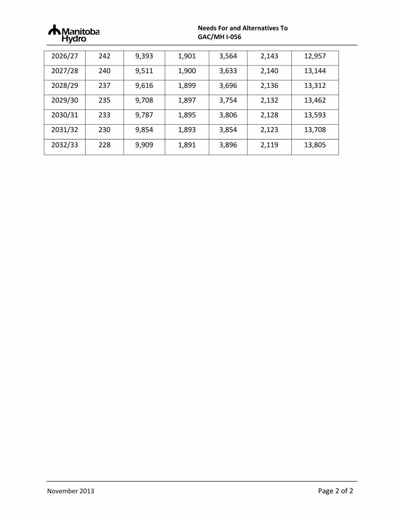
Needs For and Alternatives To GAC/MH I‐056
November 2013 Page 2 of 2
2026/27 242 9,393 1,901 3,564 2,143 12,957
2027/28 240 9,511 1,900 3,633 2,140 13,144
2028/29 237 9,616 1,899 3,696 2,136 13,312
2029/30 235 9,708 1,897 3,754 2,132 13,462
2030/31 233 9,787 1,895 3,806 2,128 13,593
2031/32 230 9,854 1,893 3,854 2,123 13,708
2032/33 228 9,909 1,891 3,896 2,119 13,805

Needs For and Alternatives To GAC/MH I‐057
November 2013 Page 1 of 2
REFERENCE: Appendix D 2013 Electric Load Forecast 1
2
QUESTION: 3
For each year of the forecast, please provide the number of space heating retrofits in areas not 4
served by gas, broken out by space heating source. 5
6
RESPONSE: 7
For each year of the 2013 forecast, the following table shows the forecast number of annual 8
retrofit space heating systems in single detached dwellings in No Gas Available areas, broken 9
out by space heating source. 10
11
Forecast Year
Electric Heat Total
Other Heat Total
2013/14 2,289 0
2014/15 2,312 0
2015/16 2,335 0
2016/17 2,358 0
2017/18 2,381 0
2018/19 2,404 0
2019/20 2,427 0
2020/21 2,450 0
2021/22 2,473 0
2022/23 2,497 0
2023/24 2,520 0
2024/25 2,543 0
2025/26 2,565 0
2026/27 2,588 0
2027/28 2,610 0

Needs For and Alternatives To GAC/MH I‐057
November 2013 Page 2 of 2
2028/29 2,632 0
2029/30 2,653 0
2030/31 2,674 0
2031/32 2,695 0
2032/33 2,716 0

Needs For and Alternatives To GAC/MH I‐058
November 2013 Page 1 of 1
REFERENCE: Appendix D 2013 Electric Load Forecast 1
2
QUESTION: 3
For each year of the forecast, please provide the average annual electricity use of heating and 4
non‐heating residential customers. 5
6
RESPONSE: 7
The average annual electricity use of heating and non‐heating residential customers is provided 8
on page 18 of the 2013 Electric Load Forecast included as Appendix D of the submission. 9

Needs For and Alternatives To GAC/MH I‐059
November 2013 Page 1 of 1
REFERENCE: Appendix D 2013 Electric Load Forecast 1
2
QUESTION: 3
Please provide the 2013 forecast of the residential water heating saturation rate. 4
5
RESPONSE: 6
The 2013 forecast of the residential water heating saturation rate is provided on page 18 of the 7
2013 Electric Load Forecast included as Appendix D of the submission. 8

Needs For and Alternatives To GAC/MH I-060
REFERENCE: Appendix D 2013 Electric Load Forecast 1
2
QUESTION: 3
Please provide the basis the 2013 projection of the electric water heating saturation rate, 4
including all data, assumptions, calculations and spreadsheets (with formulas intact) 5
6
RESPONSE: 7
The 2013 projection of electric water heat was based on the same Residential survey data used 8
for the 2012 projection described in Manitoba Hydro’s response to GAC/MH I-041. The major 9
differences from 2012 include the changes in the forecast of number of customers and the 10
adjustment to reflect the forecast effect of Manitoba Hydro’s heating fuel choice initiative as 11
outlined in Manitoba Hydro’s response to PUB/MH I-253(a). 12
13
The following two tables provide the detailed number of water heaters that formed the basis of 14
the electric water heat saturation rate. 15
November 2013 Page 1 of 4
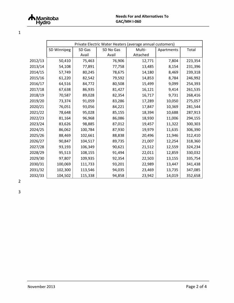
Needs For and Alternatives To GAC/MH I-060
1
Private Electric Water Heaters (average annual customers)
SD Winnipeg SD Gas Avail
SD No Gas Avail
Multi-Attached
Apartments Total
2012/13 50,410 75,463 76,906 12,771 7,804 223,354 2013/14 54,108 77,891 77,758 13,485 8,154 231,396 2014/15 57,749 80,245 78,675 14,180 8,469 239,318 2015/16 61,220 82,542 79,592 14,853 8,784 246,992 2016/17 64,516 84,772 80,508 15,499 9,099 254,393 2017/18 67,638 86,935 81,427 16,121 9,414 261,535 2018/19 70,587 89,028 82,354 16,717 9,731 268,416 2019/20 73,374 91,059 83,286 17,289 10,050 275,057 2020/21 76,051 93,056 84,221 17,847 10,369 281,544 2021/22 78,648 95,028 85,155 18,394 10,688 287,913 2022/23 81,164 96,968 86,086 18,930 11,006 294,155 2023/24 83,626 98,885 87,012 19,457 11,322 300,303 2024/25 86,062 100,784 87,930 19,979 11,635 306,390 2025/26 88,469 102,661 88,838 20,496 11,946 312,410 2026/27 90,847 104,517 89,735 21,007 12,254 318,360 2027/28 93,193 106,349 90,621 21,512 12,559 324,234 2028/29 95,513 108,155 91,494 22,011 12,859 330,032 2029/30 97,807 109,935 92,354 22,503 13,155 335,754 2030/31 100,069 111,733 93,201 22,989 13,447 341,438 2031/32 102,300 113,546 94,035 23,469 13,735 347,085 2032/33 104,502 115,338 94,858 23,942 14,019 352,658
2
3
November 2013 Page 2 of 4

Needs For and Alternatives To GAC/MH I-060
1
Other Water Heaters (average annual customers)
SD Winnipeg
SD Gas Avail
SD No Gas Avail
Multi-Attached
Apartments 2nd meter
Total
2012/13 117,307 39,105 1,957 21,701 50,547 2,310 230,617 2013/14 115,077 38,390 1,960 21,391 51,312 2,310 228,130 2014/15 112,955 37,721 1,962 21,097 52,001 2,310 225,736 2015/16 111,001 37,108 1,963 20,827 52,689 2,310 223,588 2016/17 109,221 36,560 1,965 20,581 53,376 2,310 221,703 2017/18 107,620 36,085 1,966 20,362 54,067 2,310 220,100 2018/19 106,205 35,694 1,967 20,172 54,763 2,310 218,800 2019/20 104,958 35,373 1,968 20,007 55,462 2,310 217,768 2020/21 103,825 35,088 1,968 19,857 56,163 2,310 216,902 2021/22 102,771 34,829 1,967 19,718 56,865 2,310 216,151 2022/23 101,794 34,595 1,967 19,590 57,563 2,310 215,509 2023/24 100,859 34,374 1,966 19,467 58,257 2,310 214,923 2024/25 99,938 34,156 1,964 19,345 58,945 2,310 214,349 2025/26 99,028 33,941 1,963 19,225 59,625 2,310 213,782 2026/27 98,131 33,728 1,962 19,105 60,295 2,310 213,222 2027/28 97,247 33,518 1,961 18,987 60,957 2,310 212,669 2028/29 96,367 33,310 1,959 18,869 61,608 2,310 212,114 2029/30 95,491 33,103 1,958 18,752 62,250 2,310 211,554 2030/31 94,625 32,855 1,956 18,635 62,881 2,310 210,952 2031/32 93,770 32,568 1,955 18,520 63,502 2,310 210,315 2032/33 92,925 32,283 1,953 18,406 64,115 2,310 209,682 2
The “Total” contains a small adjustment to correctly convert year-end customers to annual 3
average customers. 4
5
The following table shows the breakdown of electric water heating percentage by area and 6
dwelling type by dividing the Electric Water Heaters for each customer category by all 7
customers within each customer category (the sum of the Electric Water Heater customers and 8
the Other Water Heater customers). The final column labeled “Total” was used as the “% Elec 9
Water Heat” column in Table 14 on page 18 of the 2013 Electric Load Forecast included as 10
Appendix D of the submission. 11
November 2013 Page 3 of 4

Needs For and Alternatives To GAC/MH I-060
% Private Electric Water Heaters
SD Winnipeg
SD Gas Avail
SD No Gas Avail
Multi-Attached
Apartments Total
2012/13 30.1% 65.9% 97.5% 37.0% 13.4% 49.0% 2013/14 32.0% 67.0% 97.5% 38.7% 13.7% 50.1% 2014/15 33.8% 68.0% 97.6% 40.2% 14.0% 51.2% 2015/16 35.5% 69.0% 97.6% 41.6% 14.3% 52.2% 2016/17 37.1% 69.9% 97.6% 43.0% 14.6% 53.2% 2017/18 38.6% 70.7% 97.6% 44.2% 14.8% 54.1% 2018/19 39.9% 71.4% 97.7% 45.3% 15.1% 54.8% 2019/20 41.1% 72.0% 97.7% 46.4% 15.3% 55.6% 2020/21 42.3% 72.6% 97.7% 47.3% 15.6% 56.2% 2021/22 43.4% 73.2% 97.7% 48.3% 15.8% 56.9% 2022/23 44.4% 73.7% 97.8% 49.1% 16.1% 57.5% 2023/24 45.3% 74.2% 97.8% 50.0% 16.3% 58.0% 2024/25 46.3% 74.7% 97.8% 50.8% 16.5% 58.6% 2025/26 47.2% 75.2% 97.8% 51.6% 16.7% 59.1% 2026/27 48.1% 75.6% 97.9% 52.4% 16.9% 59.6% 2027/28 48.9% 76.0% 97.9% 53.1% 17.1% 60.1% 2028/29 49.8% 76.5% 97.9% 53.8% 17.3% 60.6% 2029/30 50.6% 76.9% 97.9% 54.5% 17.4% 61.1% 2030/31 51.4% 77.3% 97.9% 55.2% 17.6% 61.6% 2031/32 52.2% 77.7% 98.0% 55.9% 17.8% 62.0% 2032/33 52.9% 78.1% 98.0% 56.5% 17.9% 62.5%
1
November 2013 Page 4 of 4

Needs For and Alternatives To GAC/MH I-061
REFERENCE: Appendix D 2013 Electric Load Forecast; 1
2
QUESTION: 3
For each year of the forecast, please provide the system total MWh and MW assuming no 4
increase in the saturation rate of electric water heating. 5
6
RESPONSE: 7
In Order 119/13 the PUB determined that it did not require this Information Request to be 8
answered at this time. 9
November 2013 Page 1 of 1

Needs For and Alternatives To GAC/MH I‐062
November 2013 Page 1 of 2
REFERENCE: Appendix D 2013 Electric Load Forecast 1
2
QUESTION: 3
For each year of the forecast, please provide the number of new customers in gas available 4
areas, broken out by water heating source. 5
6
RESPONSE: 7
For each year of the 2013 forecast, the following table shows the numbers of new single 8
detached dwellings in Gas Available areas, broken out by water heating fuel source. 9
10
Forecast Year
Electric Water
Winnipeg
Other Water
Winnipeg
Electric Water
Gas Area
Other Water
Gas Area
Electric Water Total
Other Water Total
2013/14 1,583 11 1,787 13 3,369 24
2014/15 1,624 22 1,749 23 3,373 45
2015/16 1,624 22 1,749 23 3,373 45
2016/17 1,611 33 1,736 36 3,347 69
2017/18 1,596 55 1,720 59 3,316 115
2018/19 1,575 89 1,698 96 3,273 185
2019/20 1,563 111 1,684 119 3,246 230
2020/21 1,567 111 1,689 120 3,255 231
2021/22 1,567 111 1,689 120 3,256 231
2022/23 1,563 111 1,685 119 3,248 230
2023/24 1,555 110 1,676 119 3,231 229
2024/25 1,543 109 1,663 118 3,206 227
2025/26 1,529 108 1,647 117 3,176 225
2026/27 1,514 107 1,630 115 3,144 223
2027/28 1,497 106 1,611 114 3,109 220
2028/29 1,478 105 1,591 113 3,069 217

Needs For and Alternatives To GAC/MH I‐062
November 2013 Page 2 of 2
2029/30 1,459 103 1,569 111 3,027 214
2030/31 1,439 102 1,547 110 2,986 211
2031/32 1,421 101 1,527 108 2,948 209
2032/33 1,405 99 1,509 107 2,913 206

Needs For and Alternatives To GAC/MH I‐063
November 2013 Page 1 of 2
REFERENCE: Appendix D 2013 Electric Load Forecast 1
2
QUESTION: 3
For each year of the forecast, please provide the number of new customers in areas not served 4
by gas, broken out by water heating source. 5
6
RESPONSE: 7
For each year of the 2013 forecast, the following table shows the numbers of new single 8
detached dwellings in No Gas Available areas, broken out by water heating source. 9
10
Forecast Year
Electric Water Total
Other Water Total
2013/14 978 0
2014/15 979 0
2015/16 979 0
2016/17 978 0
2017/18 987 0
2018/19 994 0
2019/20 998 0
2020/21 999 0
2021/22 998 0
2022/23 994 0
2023/24 988 0
2024/25 979 0
2025/26 970 0
2026/27 959 0
2027/28 948 0
2028/29 935 0

Needs For and Alternatives To GAC/MH I‐063
November 2013 Page 2 of 2
2029/30 922 0
2030/31 910 0
2031/32 899 0
2032/33 888 0

Needs For and Alternatives To GAC/MH I‐064
November 2013 Page 1 of 2
REFERENCE: Appendix D 2013 Electric Load Forecast 1
2
QUESTION: 3
For each year of the forecast, please provide the number water heating retrofits in gas available 4
areas, broken out by water heating source. 5
6
RESPONSE: 7
For each year of the 2013 forecast, the following table shows the number of water heating 8
retrofits in single detached dwellings in Gas Available areas, broken out by water heating fuel 9
source. 10
11
Forecast Year
Electric Water
Winnipeg
Other Water
Winnipeg
Electric Water
Gas Area
Other Water
Gas Area
Electric Water Total
Other Water Total
2013/14 4,055 9,596 5,967 3,199 10,022 12,795
2014/15 4,326 9,435 6,152 3,141 10,478 12,576
2015/16 4,579 9,293 6,333 3,088 10,912 12,381
2016/17 4,816 9,168 6,509 3,039 11,325 12,207
2017/18 5,035 9,061 6,679 2,997 11,714 12,058
2018/19 5,240 8,970 6,844 2,961 12,084 11,931
2019/20 5,431 8,896 7,003 2,932 12,434 11,828
2020/21 5,610 8,834 7,159 2,907 12,769 11,741
2021/22 5,783 8,779 7,313 2,885 13,096 11,664
2022/23 5,949 8,731 7,464 2,864 13,413 11,595
2023/24 6,109 8,689 7,613 2,846 13,722 11,535
2024/25 6,265 8,649 7,761 2,828 14,026 11,477
2025/26 6,418 8,612 7,907 2,810 14,325 11,422
2026/27 6,568 8,576 8,052 2,792 14,620 11,368

Needs For and Alternatives To GAC/MH I‐064
November 2013 Page 2 of 2
2027/28 6,715 8,543 8,195 2,775 14,910 11,318
2028/29 6,858 8,512 8,335 2,758 15,193 11,270
2029/30 6,999 8,492 8,474 2,740 15,473 11,232
2030/31 7,137 8,474 8,611 2,725 15,748 11,199
2031/32 7,273 8,457 8,753 2,710 16,026 11,167
2032/33 7,406 8,441 8,892 2,696 16,298 11,137

Needs For and Alternatives To GAC/MH I‐065
November 2013 Page 1 of 2
REFERENCE: Appendix D 2013 Electric Load Forecast 1
2
QUESTION: 3
For each year of the forecast, please provide the number of water heating retrofits in areas not 4
served by gas, broken out by space heating source. 5
6
RESPONSE: 7
For each year of the 2013 forecast, the following table shows the number of water heating 8
retrofits in single detached dwellings in No Gas Available areas, broken out by water heating 9
fuel source. 10
11
Forecast Year
Electric Water Total
Other Water Total
2013/14 6,029 157
2014/15 6,101 157
2015/16 6,173 156
2016/17 6,245 156
2017/18 6,316 156
2018/19 6,389 156
2019/20 6,462 156
2020/21 6,535 156
2021/22 6,608 156
2022/23 6,681 156
2023/24 6,754 156
2024/25 6,826 155
2025/26 6,897 155
2026/27 6,968 155
2027/28 7,037 155

Needs For and Alternatives To GAC/MH I‐065
November 2013 Page 2 of 2
2028/29 7,106 155
2029/30 7,174 155
2030/31 7,241 155
2031/32 7,306 155
2032/33 7,371 154

Needs For and Alternatives To GAC/MH I‐066
November 2013 Page 1 of 2
REFERENCE: Appendix D 2013 Electric Load Forecast 1
2
QUESTION: 3
For each year of the forecast, provide the number of water heater retrofits where gas is 4
replaced with electric equipment. 5
6
RESPONSE: 7
For each year of the 2013 forecast, the following table shows the number of annual retrofit 8
water heating systems in single detached dwellings where natural gas is forecast to be replaced 9
with electric. 10
11
Forecast Year
Gas to Electric
Water Heat Total
2013/14 2,833
2014/15 2,695
2015/16 2,471
2016/17 2,252
2017/18 2,038
2018/19 1,831
2019/20 1,631
2020/21 1,481
2021/22 1,375
2022/23 1,272
2023/24 1,214
2024/25 1,196
2025/26 1,177
2026/27 1,159
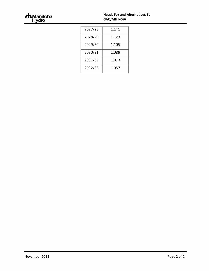
Needs For and Alternatives To GAC/MH I‐066
November 2013 Page 2 of 2
2027/28 1,141
2028/29 1,123
2029/30 1,105
2030/31 1,089
2031/32 1,073
2032/33 1,057

Needs For and Alternatives To GAC/MH I‐067
November 2013 Page 1 of 1
REFERENCE: Business Case 1
2
QUESTION: 3
Please provide documentation of Centra Gas Manitoba plans to extend accessibility to gas 4
service 5
6
RESPONSE: 7
Please refer to Manitoba Hydro’s response to MIPUG/MH I‐036d. 8

Needs For and Alternatives To GAC/MH I‐068
November 2013 Page 1 of 1
REFERENCE: Business Case 1
2
QUESTION: 3
Please provide the justification documents for the largest five Centra Gas expansions into 4
planned or existing residential areas. 5
6
RESPONSE: 7
In Order 126/13 the PUB determined that it did not require the Information Request to be 8
answered at this time. 9

Needs For and Alternatives To GAC/MH I-069
REFERENCE: Appendix D 2013 Electric Load Forecast; Page No.: 54 1
2
PREAMBLE: Manitoba Hydro expects gas heating to be cheaper than electric heating 3 throughout the forecast period 4
5
QUESTION: 6
Please explain why Manitoba Hydro expects new customers in gas available areas to opt for 7
electric space heating when the net benefits to the customer are negative. 8
9
RESPONSE: 10
As stated on page 4 of Chapter 12 of the submission and as outlined in Manitoba Hydro’s 11
response to PUB/MH I-253(a), Manitoba Hydro is projecting fewer new customers to opt for 12
electric space heat in gas available areas as a result of the heating fuel choice initiatives being 13
undertaken by Manitoba Hydro. These initiatives are outlined in Manitoba Hydro’s response to 14
PUB/MH I-253(b). 15
November 2013 Page 1 of 1

Needs For and Alternatives To GAC/MH I‐070
November 2013 Page 1 of 1
REFERENCE: Appendix D 2013 Electric Load Forecast; Page No.: 54 1
2
PREAMBLE: In the 2012 Fuel‐Switching Study, MH found gas water heating to be less 3
expensive than electric water heating 4
5
QUESTION: 6
Please explain why Manitoba Hydro expects new customers in gas‐available areas, regardless of 7
space heat fuel, to opt for electric water heating when the net benefits to the customer are 8
negative. 9
10
RESPONSE: 11
Please see Manitoba Hydro’s response to GAC/MH I‐079. 12

Needs For and Alternatives To GAC/MH I‐071
November 2013 Page 1 of 2
REFERENCE: Appendix D 2013 Electric Load Forecast; Page No.: 54 1
2
PREAMBLE: In the 2012 Fuel‐Switching Study, Manitoba Hydro found gas water 3
heating to be less expensive than electric water heating. 4
5
QUESTION: 6
Please explain why Manitoba Hydro expects existing customers, to replace gas water heaters 7
with electric water heaters when the net benefits to the customer are negative. 8
9
RESPONSE: 10
The economics for the customer depends upon their specific circumstances and whether the 11
customer is considering total costs (capital and operating) or simply considering the capital 12
cost. In many cases, customers might be primarily influenced by the upfront costs. In cases 13
where customers replace their conventional natural gas furnaces with high efficiency models, 14
the existing chimney may need to be sleeved or adjusted at an additional cost of approximately 15
$550 to adequately vent a conventional natural gas water heater. If required, this will increase 16
the cost of the installation diminishing the overall net benefit of choosing natural gas water 17
heating. 18
19
The customer will assess the choices based upon their individual circumstances, including the 20
age and condition of their existing water heater and the customer’s personal financial situation. 21
In some situations, contractors may encourage customers to install an electric water heater 22
rather than assessing the need for adjusting the venting or installing a more costly side‐venting 23
natural gas water heater. 24

Needs For and Alternatives To GAC/MH I‐071
November 2013 Page 2 of 2
The following table outlines the approximate cost of installing various hot water tank 1
alternatives: 2
Average Installed Cost
Cost of Natural Gas Option Compared to Electric
New Electric Water Heater $1,000
Existing Natural Gas Water Heater requiring Chimney Adjustment for Venting*
$550 ($450)
New Conventional Natural Gas Water Heater
$900 ($100)
New Conventional Natural Gas Water Heater requiring Chimney Adjustment for Venting
$1,450 $450
New Side‐Vent Natural Gas Water Heater $1,750 $750
*Pricing assumes the current structure is favorable for chimney sleeving or adjustments (e.g. 1 storey, minimal 3 bends in current venting). 4

Needs For and Alternatives To GAC/MH I‐072
November 2013 Page 1 of 3
REFERENCE: Appendix D 2013 Electric Load Forecast; Page No.: 11 1
2
PREAMBLE: The 2013 load forecast includes an adjustment for MH's fuel choice 3
initiatives. 4
5
QUESTION: 6
For each year of the 2013 forecast, please provide the reduction in the residential annual MWh 7
and MW due to the fuel‐choice initiatives. 8
9
RESPONSE: 10
For each year of the 2013 forecast, the following table shows the reduction in annual GWh due 11
to the fuel‐choice initiatives. 12
13
Forecast Year
New Home Space Heating GWh
Reduction
New Home Water
Heating GWh Reduction
Replacement Space Heating
GWh Reduction
Replacement Water
Heating GWh Reduction
2013/14 0.6 0.1 1.4 0.0
2014/15 1.4 0.2 2.6 0.4
2015/16 1.9 0.2 3.2 1.1
2016/17 2.7 0.2 4.6 1.7
2017/18 4.4 0.4 5.2 2.3
2018/19 6.9 0.6 5.2 2.9
2019/20 9.1 0.8 5.2 3.5
2020/21 10.5 0.8 5.2 3.9
2021/22 11.6 0.8 5.2 4.1
2022/23 13.0 0.8 5.2 4.3
2023/24 13.8 0.8 5.2 4.4

Needs For and Alternatives To GAC/MH I‐072
November 2013 Page 2 of 3
2024/25 13.7 0.8 5.2 4.3
2025/26 13.6 0.8 5.2 4.2
2026/27 13.5 0.8 5.2 4.1
2027/28 13.3 0.8 5.2 4.0
2028/29 13.2 0.7 5.2 3.9
2029/30 13.0 0.7 5.2 3.8
2030/31 12.8 0.7 5.2 3.7
2031/32 12.7 0.7 5.2 3.6
2032/33 12.5 0.7 5.2 3.5
Total 194 12 96 64
1
For each year of the 2013 forecast, the following table shows the reduction in annual MW due 2
to the fuel‐choice initiatives. 3
4
Forecast Year
New Home Space Heating MW
Reduction
New Home Water
Heating MW Reduction
Replacement Space Heating
MW Reduction
Replacement Water Heating MW
Reduction
2013/14 0.2 0.0 0.5 0.0
2014/15 0.5 0.0 0.9 0.1
2015/16 0.7 0.0 1.2 0.2
2016/17 1.0 0.0 1.6 0.3
2017/18 1.6 0.1 1.9 0.4
2018/19 2.5 0.1 1.9 0.4
2019/20 3.2 0.1 1.9 0.5
2020/21 3.7 0.1 1.9 0.6
2021/22 4.2 0.1 1.9 0.6
2022/23 4.6 0.1 1.9 0.7
2023/24 4.9 0.1 1.9 0.7

Needs For and Alternatives To GAC/MH I‐072
November 2013 Page 3 of 3
2024/25 4.9 0.1 1.9 0.7
2025/26 4.8 0.1 1.9 0.6
2026/27 4.8 0.1 1.9 0.6
2027/28 4.8 0.1 1.9 0.6
2028/29 4.7 0.1 1.9 0.6
2029/30 4.6 0.1 1.9 0.6
2030/31 4.6 0.1 1.9 0.6
2031/32 4.5 0.1 1.9 0.6
2032/33 4.5 0.1 1.9 0.5
Total 69 2 34 10

Needs For and Alternatives To GAC/MH I‐073
November 2013 Page 1 of 1
REFERENCE: Appendix D 2013 Electric Load Forecast; Page No.: 12 1
2
QUESTION: 3
Please describe Manitoba Hydro’s planned heating fuel choice initiatives 4
5
RESPONSE: 6
Please see Manitoba Hydro’s response to PUB/MH I‐253 (b). 7

Needs For and Alternatives To GAC/MH I‐074
November 2013 Page 1 of 1
REFERENCE: Appendix D 2013 Electric Load Forecast; Page No.: 12 1
2
QUESTION: 3
Please provide all reports, studies and other documentation of Manitoba Hydro's planned 4
heating fuel choice initiatives. 5
6
RESPONSE: 7
Please see Manitoba Hydro’s response to PUB/MH I‐253b. As alternative strategies are 8
currently being assessed and internal reviews have not been completed, it would be 9
inappropriate to provide the requested information. 10

Needs For and Alternatives To GAC/MH I‐075
November 2013 Page 1 of 1
REFERENCE: Appendix D 2013 Electric Load Forecast; Page No.: 12 1
2
QUESTION: 3
Please document the cost‐effectiveness analyses of Manitoba Hydro's planned heating fuel 4
choice initiatives. 5
6
RESPONSE: 7
See Manitoba Hydro’s to PUB/MH I‐253b. As alternative strategies are currently being assessed 8
and internal reviews have not been completed, it would be inappropriate to provide the 9
requested information. 10

Needs For and Alternatives To GAC/MH I‐076
November 2013 Page 1 of 1
REFERENCE: Appendix D 2013 Electric Load Forecast; Page No.: 12 1
2
QUESTION: 3
Please identify all heating fuel choice initiatives considered by the Company but rejected, and 4
provide the basis for rejection. 5
6
RESPONSE: 7
Please see Manitoba Hydro’s response to PUB/MH I‐253 (b). 8

Needs For and Alternatives To GAC/MH I‐077
November 2013 Page 1 of 2
REFERENCE: Chapter 4: The Need for New Resources; Page No.: 30 1
2
QUESTION: 3
Please identify existing and future market barriers to the installation of the least‐cost space 4
heating fuel choice. 5
6
RESPONSE: 7
The following are considered the primary barriers: 8
9 • The initial installed cost of electric heating systems is less expensive than that of natural
gas systems. Some customers do not consider total cost of ownership (i.e. capital cost 10
plus operating cost), and as such, may choose an electric heating system. In the new 11
home market, the heating system decisions are made by the homebuilder when homes 12
are built on speculation. A lower initial cost allows the homebuilder either to sell the 13
home at lower price or the opportunity to make more profit per home. In addition, 14
some builders have also indicated the additional operational benefit of not needing to 15
coordinate additional work crews associated with natural gas. 16
17 • Past volatility in natural gas markets still resonates with customers, although less so now
due to natural gas prices remaining low and declining for a number of years. Customers 18
may still be concerned that natural gas prices may increase substantially in the future as 19
the energy form is non‐renewable. Conversely, customers have experienced low and 20
modest electricity rate increases in Manitoba for decades. 21
22 • Some customers may simply not be aware of the differential in operating costs
associated with heating their homes with natural gas or electricity. 23
24 • Electricity generated in Manitoba is primarily from renewable resources and some
customers may be influenced by the environmental attractiveness from a local 25
perspective of this source of energy relative to natural gas which produces GHG 26
emissions. 27

Needs For and Alternatives To GAC/MH I‐077
November 2013 Page 2 of 2
Electricity is generated locally as opposed to natural gas which is imported from other1 •
regions. Some customers may be influenced by their desire to support the local2
economy.3
4 • Customers may be influenced by their perception related to safety in using the two
alternate sources of energy. Based on Manitoba Hydro’s Customer Satisfaction Tracking 5
Study survey conducted in April of 2013, 62% of respondents felt that electricity was 6
safer for space heating compared to 11% of customers who felt natural gas was safer. 7

Needs For and Alternatives To GAC/MH I‐078
November 2013 Page 1 of 1
REFERENCE: Business Case 1
2
QUESTION: 3
Please describe Manitoba Hydro's planned or potential efforts to eliminate market barriers to 4
the installation of the least‐cost space heating fuel choice. 5
6
RESPONSE: 7
Please see Manitoba Hydro’s response to PUB/MH I‐253 (b). 8

Needs For and Alternatives To GAC/MH I‐079
November 2013 Page 1 of 2
REFERENCE: Appendix D 2013 Electric Load Forecast; Page No.: 54 1
2
QUESTION: 3
Please explain why home builders install primarily electric water heaters. 4
5
RESPONSE: 6
Homebuilders in Manitoba primarily install electric water heaters because this is the most 7
economic option for the homebuilder and as such, it allows the homebuilder to keep the base 8
cost of the home lower, thereby the homebuilder’s competitive position in the new home 9
market. 10
11
For example, the estimated cost of installing various hot water tank options is as follows: 12
‐ $1000 to install an electric hot water tank 13
‐ $2000 to install a side‐vented natural gas hot water tank 14
A conventional natural gas hot water tank is not considered an option as it would require a 15
chimney which would reduce the useable square footage available to the homeowner or it 16
would require constructing a large home to accommodate the additional square footage 17
needed for the chimney. 18
19
Additional challenges associated with installing a side‐vented hot water tank include: 20
‐ The Manitoba Building Code has specific requirements as to where natural gas 21
appliances can be vented on the exterior walls of a home. Venting cannot be installed 22
within specified minimum distances of operable windows, exterior doors, air 23
conditioners, fresh air intakes, utility meters, cantilevers and outdoor living spaces (i.e. 24
decks or patios). 25

Needs For and Alternatives To GAC/MH I‐079
November 2013 Page 2 of 2
‐ In addition to venting restrictions by the building code, there are also aesthetic 1
limitations; e.g., customers will not be satisfied with venting being visible on the front of 2
houses. 3

Needs For and Alternatives To GAC/MH I‐080
November 2013 Page 1 of 1
REFERENCE: Appendix D 2013 Electric Load Forecast; Page No.: 54 1
2
QUESTION: 3
Please explain whether Manitoba Hydro considers developers' financial incentives to install 4
electric heating equipment to be a market barrier to cost‐effective fuel choice. 5
6
RESPONSE: 7
Please see Manitoba Hydro’s response to GAC/MH I‐077. 8

Needs For and Alternatives To GAC/MH I‐081
November 2013 Page 1 of 1
REFERENCE: Appendix D 2013 Electric Load Forecast; Page No.: 54 1
2
QUESTION: 3
Please identify all current, planned and potential efforts to discourage the installation of higher 4
cost electric heat installation in new homes in areas where gas is available. 5
6
RESPONSE: 7
Please see Manitoba Hydro’s response to PUB/MH I‐253b. 8

Needs For and Alternatives To GAC/MH I‐082
November 2013 Page 1 of 1
REFERENCE: Appendix D 2013 Electric Load Forecast; Page No.: 54 1
2
QUESTION: 3
Please explain whether Manitoba Hydro has considered putting restrictions on line extensions 4
to new developments where non‐cost‐effective electric heating is going to be installed. 5
6
RESPONSE: 7
Manitoba Hydro believes that its customers value the ability to have choice when it comes to 8
selecting their heating source and would therefore be unlikely to place restrictions on individual 9
extensions. However, Manitoba Hydro is currently examining changes to electric service 10
extension policies to establish appropriate price signals to encourage natural gas heating 11
systems in natural gas available areas. 12

Needs For and Alternatives To Round 1 GAC‐0083
November 2013 Page 1 of 1
REFERENCE: Appendix E 2013‐ 2016 Power Smart Plan; Page No.: 10 1
2
PREAMBLE: The Power Smart Residential Loan program provides financing for gas and 3
electric water and space heating equipment. 4
5
QUESTION: 6
Please indicate if this program is limited to existing customers. 7
8
RESPONSE: 9
The Power Smart Residential Loan Program is limited to existing Manitoba Hydro customers 10
who are home owners. New homes are not eligible. 11

Needs For and Alternatives To GAC/MH I‐084
November 2013 Page 1 of 2
REFERENCE: Appendix E 2013‐ 2016 Power Smart Plan 1
2
PREAMBLE: The Power Smart Residential Loan program provides financing for gas and 3
electric water and space heating equipment 4
5
QUESTION: 6
Please identify the requirements that water and space heating equipment must meet to be 7
eligible for loans. 8
9
RESPONSE: 10
Residential Water Heating Equipment must meet the following criteria for eligibility in the 11
Power Smart Residential Loan Program: 12
• Electric water heaters must meet requirements associated with Canadian Standards 13
Association C191.1 for electric storage tank water heaters 14
• Instantaneous (tankless), gas‐fired water heaters must have an energy factor (EF) of 15
0.82 or higher and be approved by the Canadian Standards Association 16
• Domestic gas‐fired water heaters must have an energy factor (EF) of 0.62 or higher and 17
be approved by the Canadian Standards Association 18
• Drain Water Heat Recovery Systems must be on a list of approved units through Natural 19
Resources Canada 20
Residential Space Heating Equipment must meet the following criteria for eligibility in the 21
Power Smart Residential Loan Program: 22
• Gas Furnaces must be a Canadian Standards Association approved high efficiency 23
condensing unit with a minimum AFUE of 92 per cent 24
• Gas Boilers must be a Canadian Standards Association approved near condensing or 25
condensing unit with a minimum AFUE of 85 per cent 26

Needs For and Alternatives To GAC/MH I‐084
November 2013 Page 2 of 2
• Electric heating systems (instantaneous and storage type) must be Canadian Standards 1
Association approved. 2

Needs For and Alternatives To GAC/MH I‐085a
November 2013 Page 1 of 1
REFERENCE: Appendix E 2013‐ 2016 Power Smart Plan 1
2
PREAMBLE: The Power Smart Residential Loan program provides financing for gas and 3
electric water and space heating equipment 4
5
QUESTION: 6
Please indicate whether a request from an existing gas customer for a loan for new electric 7
space or water heating equipment must undergo a cost‐effectiveness analysis. If so, provide an 8
example of an actual analysis. 9
10
RESPONSE: 11
Manitoba Hydro offers the Power Smart Residential Loan generally on a cost recovery basis. 12
The objective of the program is to assist customers with implementing energy efficient 13
opportunities by offering a convenient financing option. Eligibility to use the Power Smart 14
Residential Loan is not restricted to only economic opportunities and the eligible opportunities 15
are not subject to a cost‐effective analysis. 16

Needs For and Alternatives To GAC/MH I‐085b
November 2013 Page 1 of 1
REFERENCE: Appendix E 2013‐ 2016 Power Smart Plan 1
2
PREAMBLE: The Power Smart Residential Loan program provides financing for gas and 3
electric water and space heating equipment. 4
5
QUESTION: 6
Please indicate whether a request from an existing gas customer for a loan for new electric 7
space or water heating equipment must undergo a cost‐effectiveness analysis. If not, explain 8
why not. 9
10
RESPONSE: 11
Please see Manitoba Hydro’s response to GAC/MH I‐085a. 12

Needs For and Alternatives To GAC/MH I‐086
November 2013 Page 1 of 1
REFERENCE: Appendix E 2013‐ 2016 Power Smart Plan 1
2
PREAMBLE: The Power Smart Residential Loan program provides financing for gas and 3
electric water and space heating equipment. 4
5
QUESTION: 6
For every year of the program since 2001, past and projected, please provide the number and 7
total $ amount of loans for space heating equipment, by fuel type. 8
9
RESPONSE: 10
Loans issued for space heating equipment are as follows: 11
Electric Natural Gas
Total Loans Total $ Financed Loans $ Financed Loans $ Financed
2000‐01 51 $144,911 6 $16,496 45 $128,415
2001‐02 793 $2,380,507 36 $105,511 757 $2,274,996
2002‐03 642 $2,107,682 52 $124,687 590 $1,982,995
2003‐04 1096 $4,069,039 56 $147,708 1040 $3,921,331
2004‐05 1709 $6,540,181 70 $194,622 1639 $6,345,559
2005‐06 2292 $8,728,495 90 $301,363 2202 $8,427,132
2006‐07 3871 $14,548,879 87 $343,636 3784 $14,205,243
2007‐08 3447 $15,081,733 120 $472,164 3327 $14,609,569
2008‐09 3350 $16,014,768 108 $485,425 3242 $15,529,343
2009‐10 2290 $11,294,754 142 $558,635 2148 $10,736,119
2010‐11 2106 $10,199,280 144 $272,953 1962 $9,926,327
2011‐12 2091 $9,422,799 139 $344,221 1952 $9,078,578
2012‐13 1506 $6,786,906 155 $548,102 1351 $6,238,804
2013‐14 (to 09/30/2013) 449 $2,018,822 87 $155,903 362 $1,862,919
Annual estimate to 2028 1428 $6,710,935 128 $600,935 1300 $6,110,000
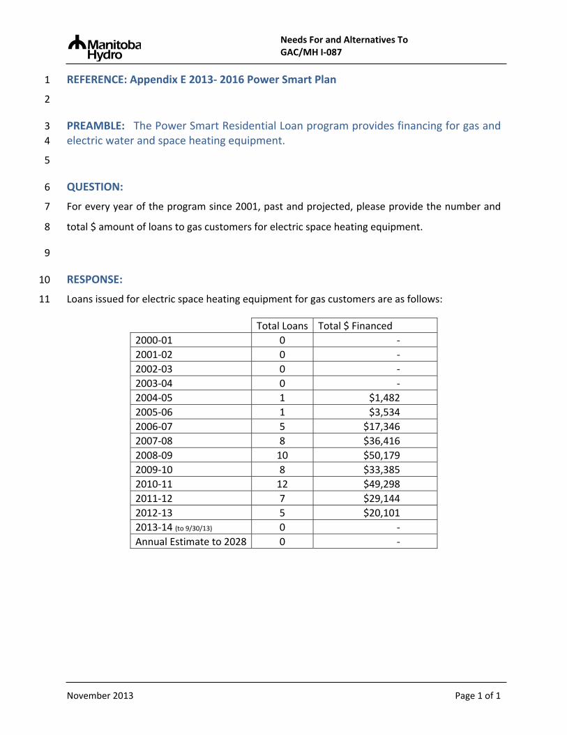
Needs For and Alternatives To GAC/MH I‐087
November 2013 Page 1 of 1
REFERENCE: Appendix E 2013‐ 2016 Power Smart Plan 1
2
PREAMBLE: The Power Smart Residential Loan program provides financing for gas and 3
electric water and space heating equipment. 4
5
QUESTION: 6
For every year of the program since 2001, past and projected, please provide the number and 7
total $ amount of loans to gas customers for electric space heating equipment. 8
9
RESPONSE: 10
Loans issued for electric space heating equipment for gas customers are as follows: 11
Total Loans Total $ Financed
2000‐01 0 ‐
2001‐02 0 ‐
2002‐03 0 ‐
2003‐04 0 ‐
2004‐05 1 $1,482
2005‐06 1 $3,534
2006‐07 5 $17,346
2007‐08 8 $36,416
2008‐09 10 $50,179
2009‐10 8 $33,385
2010‐11 12 $49,298
2011‐12 7 $29,144
2012‐13 5 $20,101
2013‐14 (to 9/30/13) 0 ‐
Annual Estimate to 2028 0 ‐

Needs For and Alternatives To GAC/MH I‐088
November 2013 Page 1 of 1
REFERENCE: Appendix E 2013‐ 2016 Power Smart Plan 1
2
PREAMBLE: The Power Smart Residential Loan program provides financing for gas and 3
electric water and space heating equipment. 4
5
QUESTION: 6
For every year of the program since 2001, past and projected, please provide the number and 7
total $ amount of loans for water heating equipment, by fuel type. 8
9
RESPONSE: 10
Prior to 2009, Manitoba Hydro only tracked primary equipment (e.g. furnace, windows, etc) 11
being financed through the program. Since then; data collection was modified to differentiate 12
by the energy efficient measure installed under each loan application. The following activity for 13
water heating equipment is available beginning in 2009/10: 14
Electric Natural Gas
Total Loans Total $ Financed Loans $ Financed Loans $ Financed
2009‐10 104 $107,662 15 $12,966 89 $94,696
2010‐11 44 $45,608 14 $12,949 30 $32,659
2011‐12 85 $91,529 27 $23,914 58 $67,615
2012‐13 47 $53,352 15 $13,248 32 $40,104
2013‐14 (to 30/09/2013) 117 $128,643 83 $82,671 34 $45,972
Annual estimate to 2028 42 $45,402 15 $13,707 27 $31,695

Needs For and Alternatives To GAC/MH I‐089
November 2013 Page 1 of 1
REFERENCE: Appendix E 2013‐ 2016 Power Smart Plan 1
2
PREAMBLE: The Power Smart Residential Loan program provides financing for gas and 3
electric water and space heating equipment. 4
5
QUESTION: 6
For every year of the program since 2001, past and projected, please provide the number and 7
total $ amount of loans to gas water heating customers for electric water heating equipment. 8
9
RESPONSE: 10
Information regarding the water heating equipment being removed from the home is not 11
collected as part of the loan application process for the Power Smart Residential Loan. 12
Information collected focuses on ensuring the new equipment to be financed meets qualifying 13
energy efficiency standards. As a result, the requested information is not available. 14

Needs For and Alternatives To GAC/MH I‐090
November 2013 Page 1 of 1
REFERENCE: Appendix E 2013‐ 2016 Power Smart Plan; Page No.: 11 1
2
PREAMBLE: Power Smart PAYS Financing provides financing for gas and electric space 3
heating equipment. 4
5
QUESTION: 6
Please indicate if this program is limited to existing customers. 7
8
RESPONSE: 9
The Residential PAYS Financing Program is available to existing and new Manitoba Hydro 10
customers.11

Needs For and Alternatives To GAC/MH I‐091
November 2013 Page 1 of 1
REFERENCE: Appendix E 2013‐ 2016 Power Smart Plan 1
2
QUESTION: 3
Please identify the requirements that the space heating equipment must meet to be eligible for 4
loans. 5
6
RESPONSE: 7
In order to finance space heating equipment under the Residential PAYS Financing Program, the 8
monthly payment for the funds borrowed from Manitoba Hydro must be less than the 9
estimated average monthly utility bill savings. Space heating equipment must also meet the 10
following technical requirements to be eligible for financing: 11
• Gas Furnaces must be a Canadian Standards Association approved high efficiency 12
condensing unit with a minimum AFUE of 92 per cent 13
• Gas Boilers must be a Canadian Standards Association approved near condensing or 14
condensing unit with a minimum AFUE of 85 per cent 15
• A Canadian Standards Association approved electric furnace, electric boiler, or electric 16
baseboard heat when it is the primary heating source (existing homes only) 17
• Geothermal heat pump system must be tested and rated under Canadian Standards 18
Association C‐13256 and installed to meet Canadian Standards Association C448 19
Additionally, the heat pump must be designed and installed by a certified contractor 20
who is recognized by the Manitoba Geothermal Energy Alliance 21

Needs For and Alternatives To GAC/MH I‐092
November 2013 Page 1 of 1
REFERENCE: Appendix E 2013‐ 2016 Power Smart Plan 1
2
PREAMBLE: According to the Power Smart Plan, "To qualify [for PAYS], upgrades must 3
have sufficient estimated annual utility bill savings to offset the monthly financing 4
payment." 5
6
QUESTION: 7
Please provide the calculation of estimated bill savings. 8
9
RESPONSE: 10
The calculation of estimated bill savings is determined by estimating the difference between 11
what a customer’s average annual utility bill would be after implementing an energy efficient 12
measure relative to the customer’s current average annual utility bill. The estimate is 13
determined by information the customer provides regarding their project such as: home type, 14
home size, home age, existing technology, and proposed technology. Customers can determine 15
the approximate bill savings associated with their project by visiting the PAYS online calculator 16
at www.hydro.mb.ca/pays. As an example, the formula for estimating the bill saving by 17
installing a high efficiency natural gas heating system is as follows: 18
19
Monthly energy savings in dollars = (annual operating cost of a existing system ‐ annual 20
operating cost of new system) / 12 months 21
22
Annual operating cost of existing system: 23
(Energy Consumption per Square Foot of Building Type by Vintage x Current Energy Rate) x Building Size (Sq.ft) 24
Seasonal Efficiency of Existing System 25
26
Annual operating cost of new system: 27
(Energy Consumption per Square Foot of Building Type by Vintage x Current Energy Rate) x Building Size (Sq.ft) 28
Seasonal Efficiency of New System29

Needs For and Alternatives To GAC/MH I‐093
November 2013 Page 1 of 2
REFERENCE: Appendix E 2013‐ 2016 Power Smart Plan; 1
2
PREAMBLE: According to the Power Smart Plan, "To qualify [for PAYS], upgrades must 3
have sufficient estimated annual utility bill savings to offset the monthly financing 4
payment." 5
6
QUESTION: 7
In the case of a switch from gas to electric heat, please explain how the calculation of bill 8
savings reflects the difference in fuel costs, including all formula and assumptions relied upon. 9
10
RESPONSE: 11
The calculation of estimated bill savings is generated by estimating the customer’s current 12
average annual utility bill and their proposed average annual utility bill based on current utility 13
rates after the upgrade (see Manitoba Hydro’s response to Round 1 GAC‐0092). The estimate is 14
determined by information the customer provides regarding their project such as: home type, 15
home size, home age, existing technology, and proposed technology. Additionally, customers 16
are asked if they will have their natural gas service removed to account for the basic monthly 17
charge for natural gas. In the case of a switch from natural gas to electric heat, bill savings 18
results are negative and therefore, is not an eligible upgrade under the Residential PAYS 19
Financing Program. See example below: 20
21
Example: 22
A Manitoba Hydro customer would like to remove their existing standard efficiency natural gas 23
furnace and obtain financing for an electric furnace through PAYS. The customer has a 24
bungalow built in 1973 that is 1200 square feet and plans on having their natural gas service 25
removed. Based on current electric and natural gas rates, the customer‘s estimated average 26
monthly utility bill would increase by $22.33 and therefore is not eligible for financing. 27

Needs For and Alternatives To GAC/MH I‐093
November 2013 Page 2 of 2
Calculation details: 1
2
Annual operating cost of existing system: 3
(1.19 m3 per square feet for 1970‐present bungalow x $0.2597/m3) x 1200 square feet 4
0.60 Seasonal Efficiency 5
= $620 per year for existing system 6
7
Annual operating cost of new system: 8
(12.30 kw.h per square feet for 1970‐present bungalow x $0.07183/kw.h) x 1200 square feet 9
1.00 Seasonal Efficiency 10
=$1056 per year for new system 11
12
Monthly energy savings in dollars = ($620 ‐ $1056 / 12) + $14** (basic monthly charge for 13
natural gas savings) 14
= ‐ 22.33 15
16
**If the customer removes their natural gas service, they receive an additional bill savings as they will no longer be 17
paying the basic monthly service charge for natural gas. 18

Needs For and Alternatives To GAC/MH I‐094a
November 2013 Page 1 of 1
REFERENCE: Appendix E 2013‐ 2016 Power Smart Plan 1
2
PREAMBLE: According to the Power Smart Plan, "To qualify [for PAYS], upgrades must 3
have sufficient estimated annual utility bill savings to offset the monthly financing 4
payment." 5
6
QUESTION: 7
Please indicate whether a request from an existing gas customer for a loan for electric space 8
heating equipment must undergo any cost‐effectiveness analysis other than a Customer Cost 9
Test. If so, document the required analysis. 10
11
RESPONSE: 12
A utility cost‐effectiveness analysis is not required however a bill impact calculation is required. 13
Note that with the switch from a natural gas heating system to an electric heating system there 14
is a net increase to the customer’s bill and therefore the upgrade would not be eligible for 15
financing under the Residential PAYS Program. 16

Needs For and Alternatives To GAC/MH I‐094b
November 2013 Page 1 of 1
REFERENCE: Appendix E 2013‐ 2016 Power Smart Plan 1
2
PREAMBLE: According to the Power Smart Plan, "To qualify [for PAYS], upgrades must 3
have sufficient estimated annual utility bill savings to offset the monthly financing 4
payment." 5
6
QUESTION: 7
Please indicate whether a request from an existing gas customer for a loan for electric space 8
heating equipment must undergo any cost‐effectiveness analysis other than a Customer Cost 9
Test. If not, explain why not. 10
11
RESPONSE: 12
The only test that is required for eligibility under the Residential PAYS Financing Program is a 13
bill impact calculation. In the case of a switch from natural gas to electric heat, the bill impact 14
calculation is negative and is therefore not an eligible upgrade under the Residential PAYS 15
Financing Program. Please see Manitoba Hydro’s response to GAC/MH I‐093 for an example of 16
this calculation. 17

Needs For and Alternatives To GAC/MH I‐095
November 2013 Page 1 of 1
REFERENCE: Appendix E 2013‐ 2016 Power Smart Plan 1
2
PREAMBLE: According to the Power Smart Plan, "To qualify [for PAYS], upgrades must 3
have sufficient estimated annual utility bill savings to offset the monthly financing 4
payment." 5
6
QUESTION: 7
For every projection year 2012/13 to 2015/16, please provide the number and $ amount of 8
loans for space heating equipment, by fuel type. 9
10
RESPONSE: 11
The number and dollar amount of loans projected for space heating equipment under the 12
Residential PAYS Financing Program is as follows: 13
Fuel Type
2012/13 Participation
(actual)
2013/14 Participation (projected)
2014/15 Participation (projected)
2015/16 Participation (projected)
# $ # $ # $ # $
Gas: 47 $191,034 300 $1,219,365 300 $1,219,365 300 $1,219,365
Geothermal: 1 $20,000 5 $100,000 5 $100,000 5 $100,000
Total: 48 $211,034 305 $1,319,365 305 $1,319,365 305 $1,319,365
14

Needs For and Alternatives To GAC/MH I‐096
November 2013 Page 1 of 1
REFERENCE: Appendix E 2013‐ 2016 Power Smart Plan 1
2
PREAMBLE: According to the Power Smart Plan, "To qualify [for PAYS], upgrades must 3
have sufficient estimated annual utility bill savings to offset the monthly financing 4
payment." 5
6
QUESTION: 7
For every projection year 2012/13 to 2015/16, please provide the number and $ amount of 8
loans to gas customers for electric space heating equipment. 9
10
RESPONSE: 11
There are zero loans projected for natural gas customers installing electric heating equipment. 12
Switching from natural gas space heating equipment to electric space heating equipment 13
results in a bill increase and therefore does not pass the bill impact calculation for eligibility in 14
the PAYS Program. 15

Needs For and Alternatives To GAC/MH I‐097
November 2013 Page 1 of 1
REFERENCE: Appendix E 2013‐ 2016 Power Smart Plan 1
2
QUESTION: 3
Please identify all potential programs screened for the Power Smart Plan that are targeted at 4
non‐cost‐effective fuel‐switching. 5
6
RESPONSE: 7
Please see Manitoba Hydro’s response to PUB/MH I‐253 (b). 8

Needs For and Alternatives To GAC/MH I‐098
November 2013 Page 1 of 1
REFERENCE: Appendix E 2013‐ 2016 Power Smart Plan 1
2
QUESTION: 3
Please provide Manitoba Hydro’s evaluation of the cost‐effectiveness of potential programs 4
that are targeted at non‐cost‐effective fuel‐switching. 5
6
RESPONSE: 7
Please see Manitoba Hydro’s response to PUB/MH I‐253 b. 8
9
Manitoba Hydro is currently in the process of assessing the merits of undertaking programs 10
which go beyond simply an educational approach. No such programs exist today and therefore, 11
the evaluation of the cost‐effectiveness of those contemplated programs is not available. 12

Needs For and Alternatives To GAC/MH I‐099
November 2013 Page 1 of 1
REFERENCE: Business Case 1
2
QUESTION: 3
Please provide MH's update to its Manitoba Hydro's Report on the Environmental and 4
Economic Impacts of Fuel Switching in response to Directive 17 of PUB Orders 116/08 and 5
150/08, if available. 6
7
RESPONSE: 8
Manitoba Hydro has not updated the report. The “Economic, Load, and Environmental Impacts 9
of Fuel Switching in Manitoba” Report dated 16 August 2012 is the most current version of this 10
report.11

Needs For and Alternatives To GAC/MH I‐100
November 2013 Page 1 of 1
REFERENCE: Appendix E 2013‐ 2016 Power Smart Plan 1
2
QUESTION: 3
Please provide the MH's current avoided cost estimates used for DSM screening, broken down 4
by MH system cost component. 5
6
RESPONSE: 7
Manitoba Hydro’s current marginal cost of 6.69 cents (2012$s) per kWh includes all generation 8
net production costs and all capital costs associated with transmission and distribution. This 9
value has been noted in Chapter 4 – The Need for New Resources (Figure 4.12) and applied in 10
the 2013 ‐ 2016 Power Smart Plan. The annual all‐in forecast marginal cost using Manitoba 11
Hydro’s established methodology is levelized over the 30‐year period from 2013/14 to 2042/43 12
in 2012 constant year dollars. 13
14
Annual marginal costs for each major sector/end use are provided as blended average marginal 15
cost values, as follows: 16
a) At the generation level, the blended average marginal cost is 5.31¢/kWh 17
b) At the transmission level, the blended average marginal cost is 0.63¢/kWh 18
c) At the distribution level, the blended average marginal cost is 0.75¢/kWh 19

Needs For and Alternatives To GAC/MH I‐101
November 2013 Page 1 of 1
REFERENCE: Appendix E 2013‐ 2016 Power Smart Plan 1
2
QUESTION: 3
Please document the derivation of avoided cost for DSM screening, including all workpapers 4
and electronic spreadsheets (with formulas intact). 5
6
RESPONSE: 7
A general description of the derivation of generation marginal costs was provided in the NFAT 8
submission in Appendix 9.3 Economic Evaluation, Section 1.8 Description of Marginal Costs. 9
Provision of all workpapers and electronic spreadsheets would result in the disclosure of 10
commercially sensitive information. 11

Needs For and Alternatives To GAC/MH I‐102
November 2013 Page 1 of 1
REFERENCE: Appendix E 2013‐ 2016 Power Smart Plan 1
2
QUESTION: 3
Please provide the Company's most recent estimates of avoided or marginal cost by season and 4
by time of day, broken out by system cost component. 5
6
RESPONSE: 7
Please see Manitoba Hydro’s response to GAC/MH I‐100. Seasonal marginal costs cannot be 8
provided since it would require the disclosure of commercially sensitive information. 9
10
Marginal costs are not available by time of day. 11

Needs For and Alternatives To GAC/MH I‐103
November 2013 Page 1 of 1
REFERENCE: Appendix E 2013‐ 2016 Power Smart Plan; 1
2
QUESTION: 3
Please provide Hydro’s current estimates of avoided T&D costs. 4
5
6 RESPONSE:
7 The current estimates of Transmission and Distribution marginal costs in 2012 dollars are as
8 follows:
9 • Transmission: $55.35/kW/yr
10 • Distribution: $66.00/kW/yr

Needs For and Alternatives To GAC/MH I-104
REFERENCE: Appendix E 2013- 2016 Power Smart Plan; 1
2
QUESTION: 3
Please provide the derivation of Hydro’s current estimates of avoided T&D costs, including 4
studies, workpapers, and Excel spreadsheets (with formulas intact). 5
6
RESPONSE: 7
The derivation of the current estimates of transmission and distribution marginal costs is based 8
on the methodology that is provided in the attached report “2009 Marginal Transmission and 9
Distribution Cost Estimates. SPD 2010/02” Manitoba Hydro, February 11, 2013. Related 10
supporting electronic information requested is not readily available for inclusion in this 11
Information Request. 12
November2013 Page 1 of 1

Needs For and Alternatives To GAC/MH I‐105
November 2013 Page 1 of 1
REFERENCE: Appendix E 2013‐ 2016 Power Smart Plan 1
2
QUESTION: 3
Please provide Hydro’s current estimates of avoided generation plant and OM&A costs. 4
5
RESPONSE: 6
Forecast marginal cost using Manitoba Hydro established methodology and levelized over the 7
30‐year period from fiscal year 2013/14 to 2042/43 is 6.69 cents per kWh in 2012 constant year 8
dollars. This includes all generation costs and all capital costs associated with transmission and 9
distribution.10

Needs For and Alternatives To GAC/MH I‐106
November 2013 Page 1 of 1
REFERENCE: Appendix E 2013‐ 2016 Power Smart Plan 1
2
QUESTION: 3
Please provide the derivation of MH’s current estimates of avoided generation plant and OM&A 4
costs, including all workpapers and electronic spreadsheets (with formulas intact). 5
6
RESPONSE: 7
A general description of the derivation of generation marginal costs was provided in the main 8
submission in Appendix 9.3 – Economic Evaluation, Section 1.8 ‐ Description of Marginal Costs. 9
10
Manitoba Hydro does not generally provide electronic spreadsheets. Provision of all 11
workpapers and electronic spreadsheets would result in the disclosure of commercially 12
sensitive information. 13
Needs For and Alternatives To GAC/MH I‐107
November 2013 Page 1 of 1
REFERENCE: Appendix E 2013‐ 2016 Power Smart Plan 1
2
QUESTION: 3
Please provide in an Excel spreadsheet the output of each existing generation plant with and 4
without exports for the next ten years. 5
6
RESPONSE: 7
The generating capability of each generating station is not dependent on exports. The capability 8
of each existing generating station can be found in Chapter 5 Table 5.1, page 3 of the NFAT 9
Business Case and, as shown, varies with system inflow. Without export capability, river flow 10
that would result in generation surplus to Manitoba requirements would be directed over the 11
spillway.12