Near-optimal Nonmyopic Value of Information in

Graphical Models

Andreas Krause, Carlos Guestrin

Computer Science Department

Carnegie Mellon University

Applications for sensor selection

Medical domain select among potential examinations

Sensor networks observations drain power, require storage

Feature selection select most informative attributes for classification, regression etc.

...

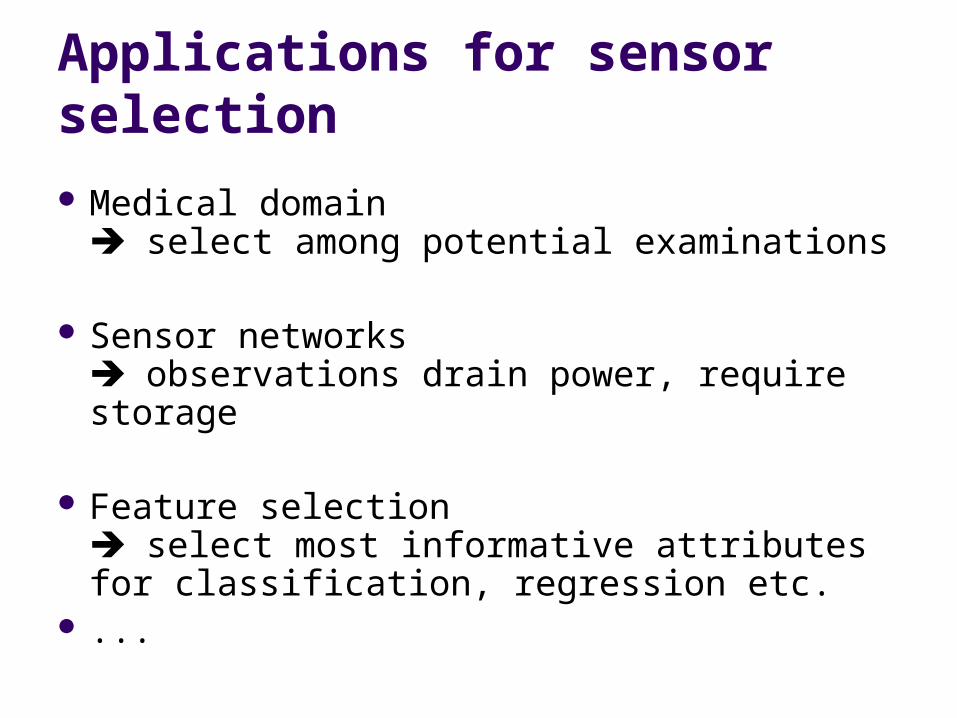
An example: Temperature prediction

SERVER

LAB

KITCHEN

COPYELEC

PHONEQUIET

STORAGE

CONFERENCE

OFFICEOFFICE50

51

52 53

54

46

48

49

47

43

45

44

42 41

3739

38 36

33

3

6

10

11

12

13 14

1516

17

19

2021

22

242526283032

31

2729

23

18

9

5

8

7

4

34

1

2

3540

Estimating temperature in a building

Wireless sensors with limited battery

T1

T2

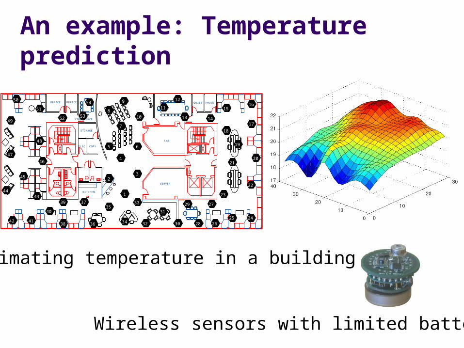
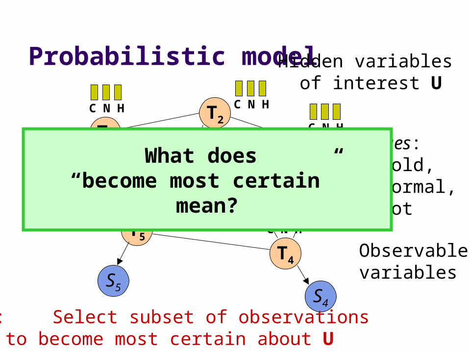
Probabilistic model

T5

T4

T3

S5

S2

S4

S3

S1

Hidden variables of interest U

Observable variables O

Task:Select subset of observations to become most certain about U

Values: (C)old, (N)ormal, (H)ot

C N HC N H

C N H

C N H

C N H

What does “become most certain”

mean?

T1

T2

Making observations

T1

T2

T5

T4

T3

S5

S2

S4

observed

Reward = 0.2

C N H

C N H

C N H

S1=hotS3

C N H

C N H

S1

C N HC N H

C N H

C N H

C N H

T2

T4

T3

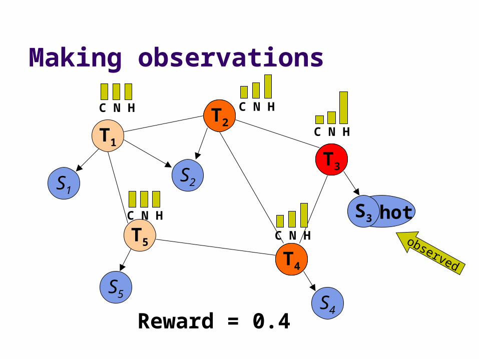
Making observations

T1

T2

T5

T4

T3

S5

S1S2

S4

S3=hot

observed

Reward = 0.4

C N H

C N H

C N H

C N H

C N H

S3

T2

T3

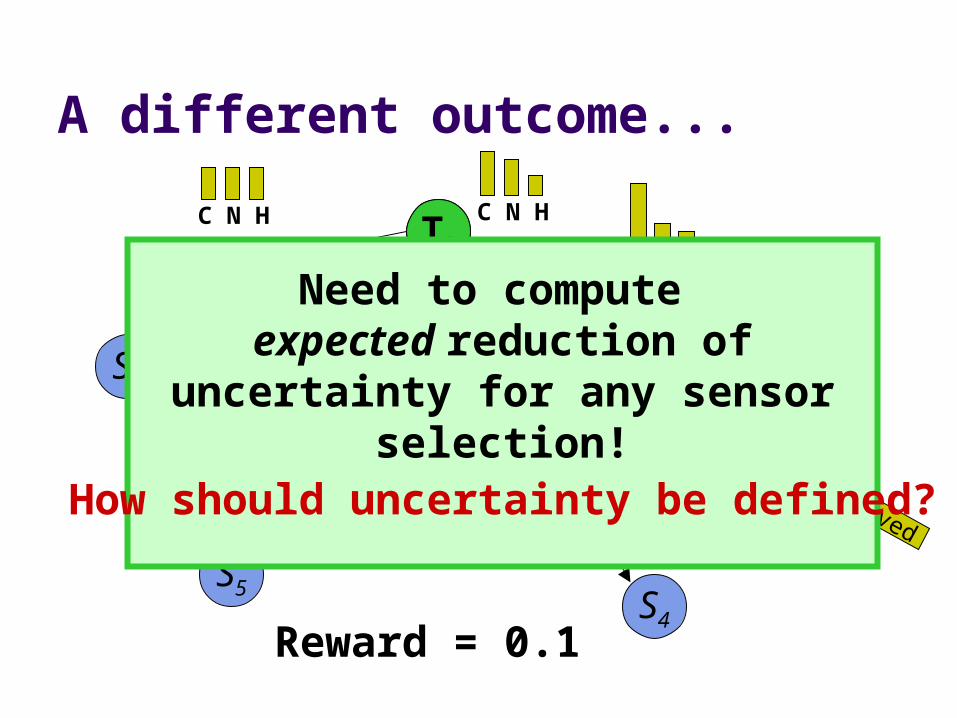
A different outcome...

T1

T2

T5

T4

T3

S5

S1S2

S4

S3=cold

Reward = 0.1

observed

C N H

C N HC N H

C N H

C N H

Need to compute expected reduction of uncertainty

for any sensor selection!

How should uncertainty be defined?

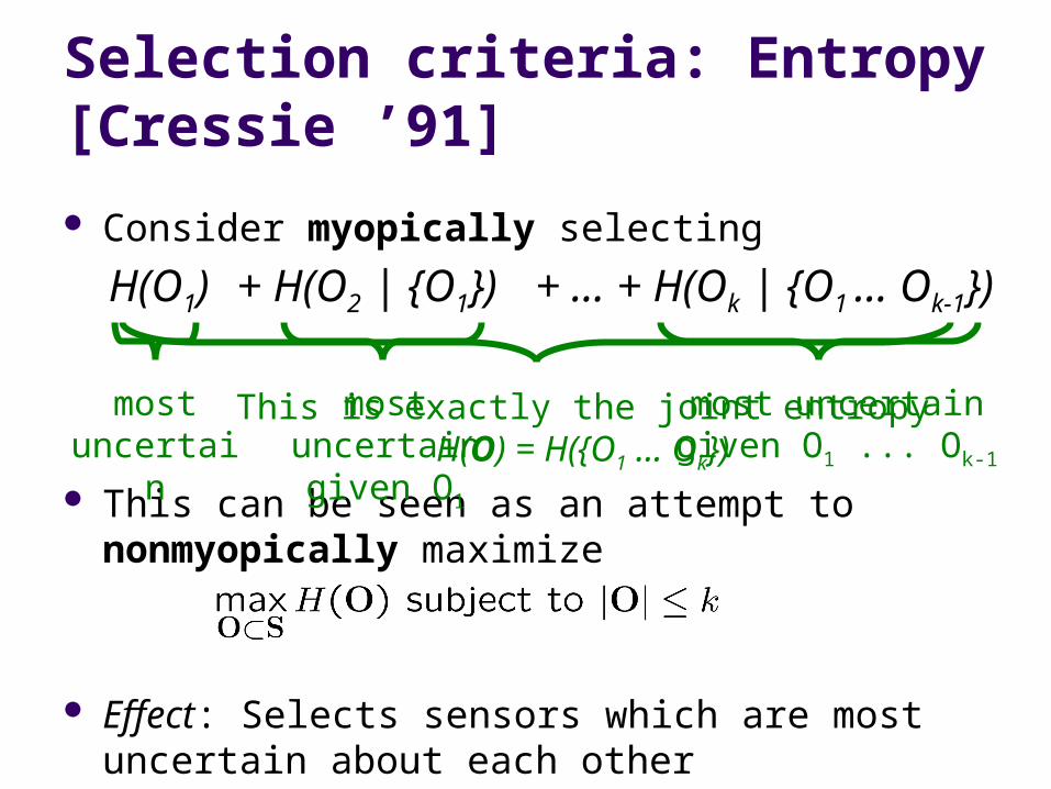
Consider myopically selecting

This can be seen as an attempt to nonmyopically maximize

Effect: Selects sensors which are most uncertain about each other

Selection criteria: Entropy [Cressie ’91]

H(O1) + H(O2 | {O1}) + ... + H(Ok | {O1 ... Ok-1})

most uncertain

most uncertaingiven O1

most uncertaingiven O1 ... Ok-1

This is exactly the joint entropyH(O) = H({O1 ... Ok})

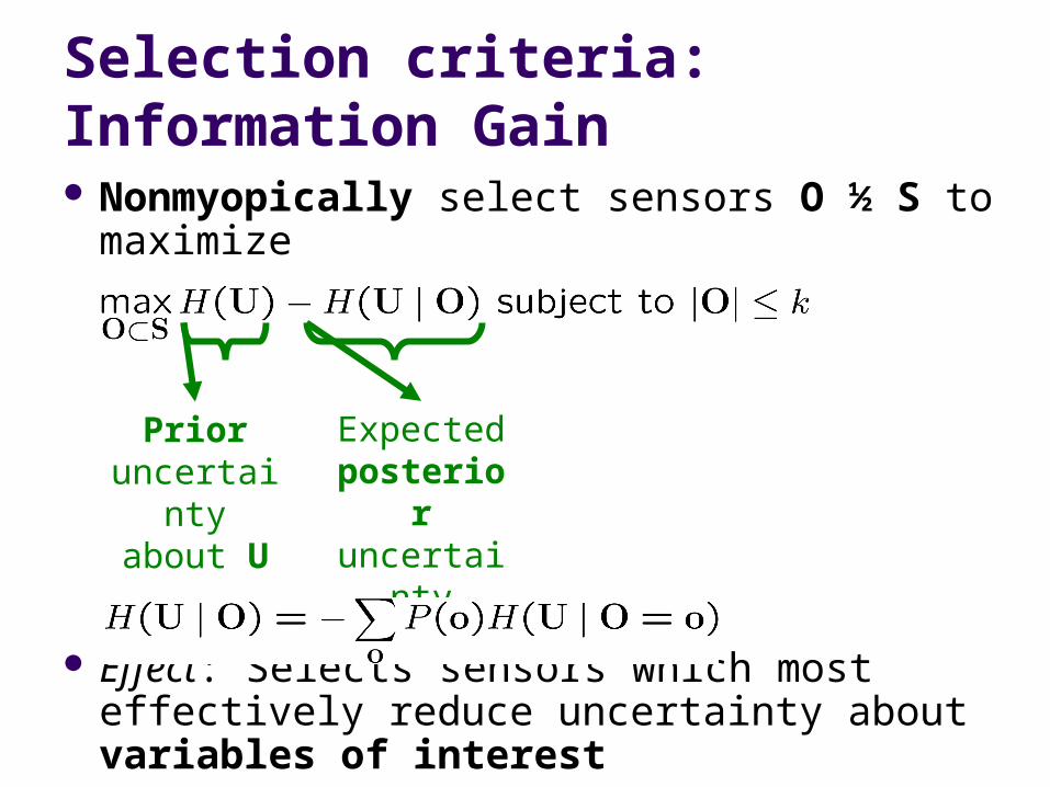
Nonmyopically select sensors O ½ S to maximize

Effect: Selects sensors which most effectively reduce uncertainty about variables of interest

Selection criteria: Information Gain

Expectedposterioruncertaint

yabout U

Prioruncertain

tyabout U

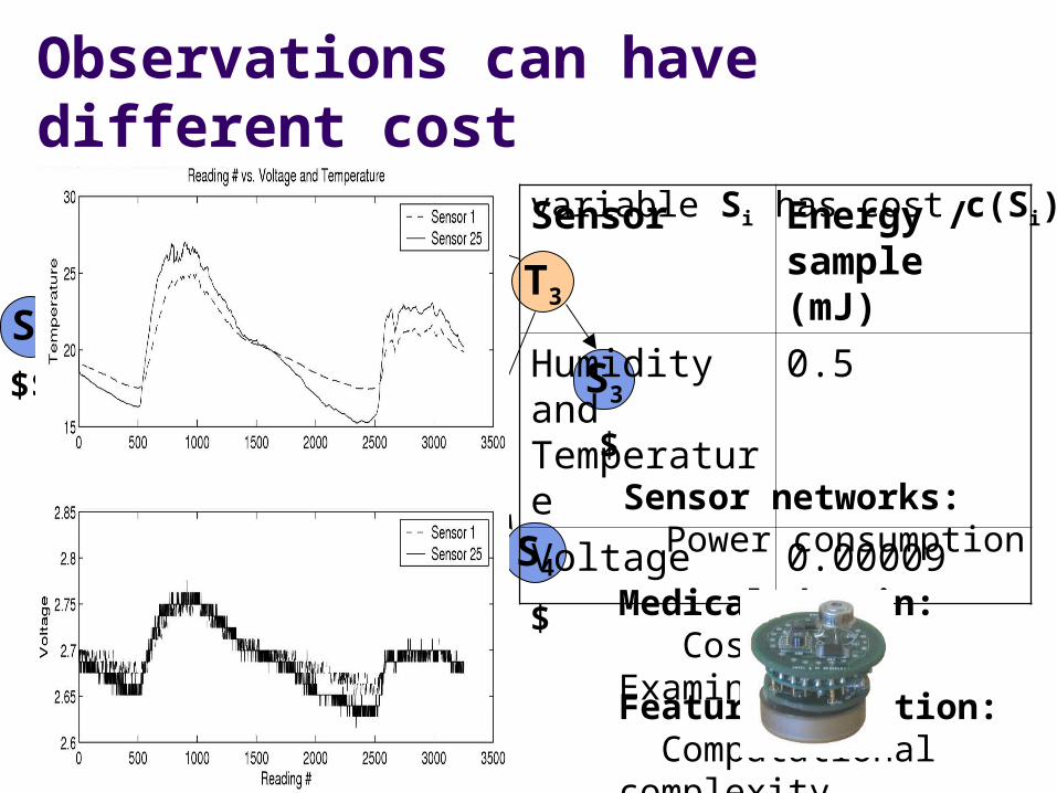
Observations can have different cost

T1

T2

T5

T4

T3

S5

S1S2

S4

S3$$$

$$

$$

$$

$

Sensor networks: Power consumption

Each variable Si has cost c(Si)

Medical domain: Cost of Examinations

Feature selection: Computational complexity

Sensor Energy / sample (mJ)

Humidity and Temperature

0.5

Voltage 0.00009

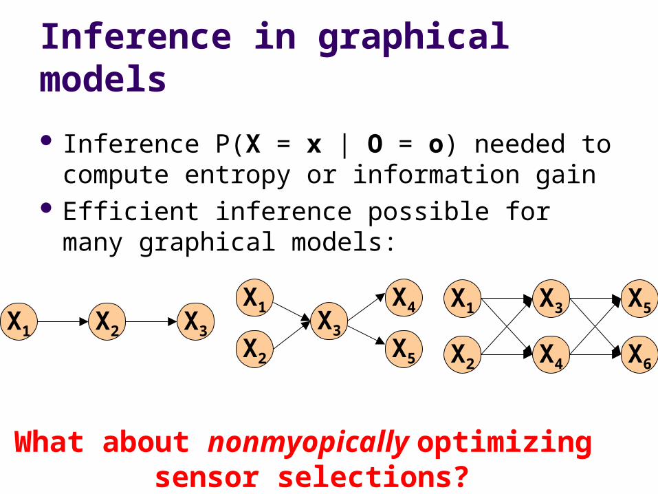
Inference in graphical models

Inference P(X = x | O = o) needed to compute entropy or information gain

Efficient inference possible for many graphical models:

X1 X2 X3 X3

X1

X2

X4

X5

X1 X3 X5

X2 X4 X6

What about nonmyopically optimizing sensor selections?

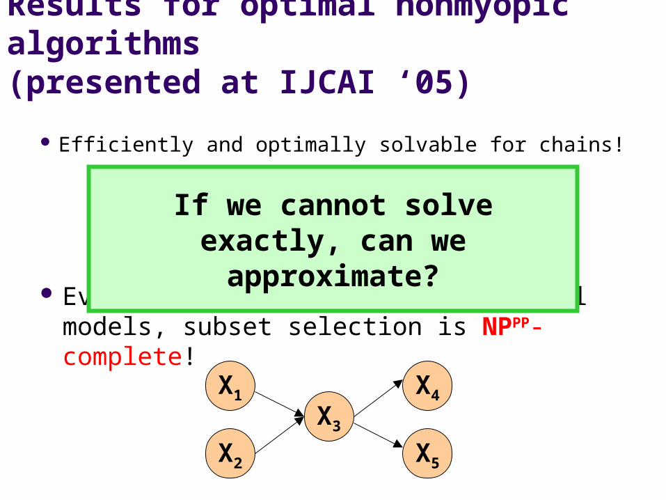
Results for optimal nonmyopic algorithms

(presented at IJCAI ‘05)

Efficiently and optimally solvable for chains!

X1 X2 X3

X3

X1

X2

X4

X5

Even on discrete polytree graphical models, subset selection is NPPP-complete!

butIf we cannot solve exactly, can

we approximate?

T1

T2

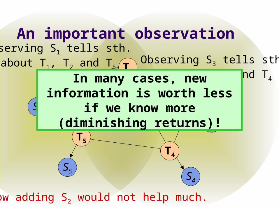
An important observation

T5

T4

T3

S5

S2

S4

S3

S1

Observing S1 tells sth.about T1, T2 and T5

Observing S3 tells sth.about T3, T2 and T4

Now adding S2 would not help much.

In many cases, new information is worth less if we know more

(diminishing returns)!

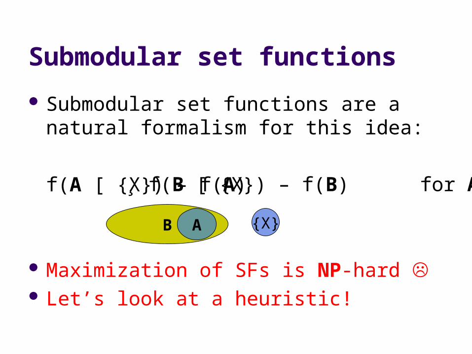
Submodular set functions

Submodular set functions are a natural formalism for this idea:

f(A [ {X}) – f(A)

Maximization of SFs is NP-hard Let’s look at a heuristic!

B A {X}

¸ f(B [ {X}) – f(B) for A µ B

S1

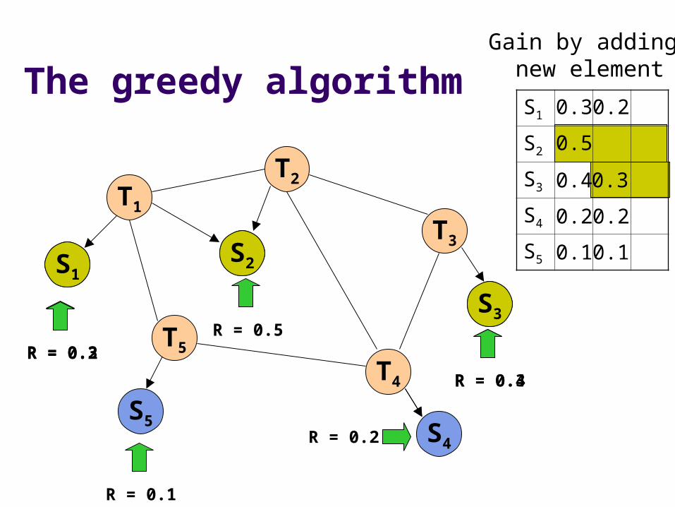
The greedy algorithm

T1

T2

T5

T4

T3

S5

S1S2

S4

S3

R = 0.3R = 0.5

R = 0.4

R = 0.2

R = 0.1

S2

R = 0.2

R = 0.3

S3

S1

S2

S3

S4

S5

0.3

0.5

0.4

0.2

0.1

0.2

0.3

0.2

0.1

Gain by adding new element

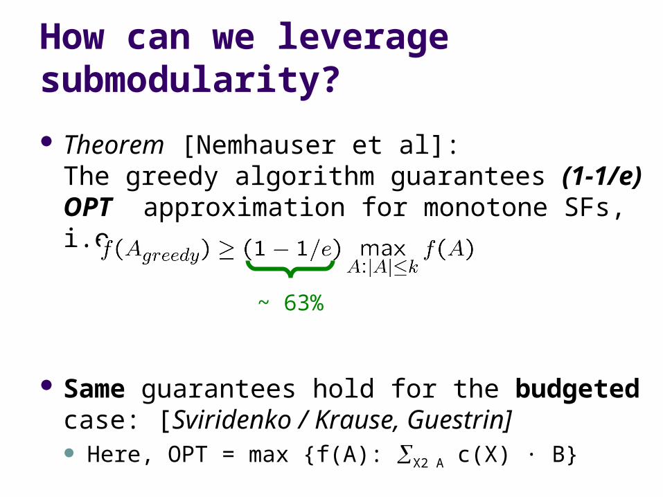
How can we leverage submodularity?

Theorem [Nemhauser et al]: The greedy algorithm guarantees (1-1/e) OPT approximation for monotone SFs, i.e.

Same guarantees hold for the budgeted case: [Sviridenko / Krause, Guestrin] Here, OPT = max {f(A): X2 A c(X) · B}

~ 63%

How can we leverage submodularity?

Theorem [Nemhauser et al]: The greedy algorithm guarantees (1-1/e) OPT approximation for monotone SFs, i.e.

Same guarantees hold for the budgeted case: [Sviridenko / Krause, Guestrin] Here, OPT = max {f(A): X2 A c(X) · B}

~ 63%

Are our objective functions submodular and monotonic?

(Discrete) Entropy is! [Fujishige ‘78]

However, entropy can waste information:

“Wasted” information

H(O1) + H(O2 | {O1}) + ... + H(Ok | {O1 ... Ok-1})

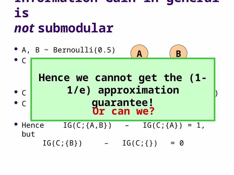
Information Gain in general is not submodular

A, B ~ Bernoulli(0.5) C = A XOR B

C | A and C | B ~ Bernoulli(0.5) (entropy 1) C | A,B is deterministic! (entropy 0)

Hence IG(C;{A,B}) – IG(C;{A}) = 1, butIG(C;{B}) – IG(C;{}) = 0

A

C

B

Hence we cannot get the (1-1/e) approximation guarantee!

Or can we?

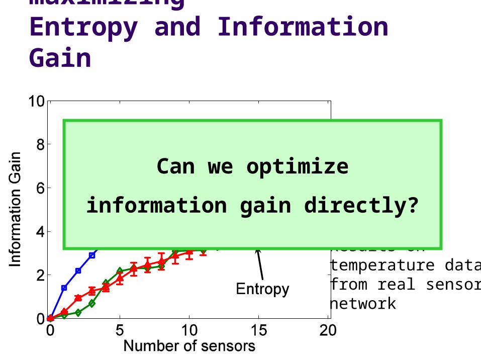
Conflict between maximizingEntropy and Information Gain

Results ontemperature datafrom real sensor network

Can we optimize

information gain directly?

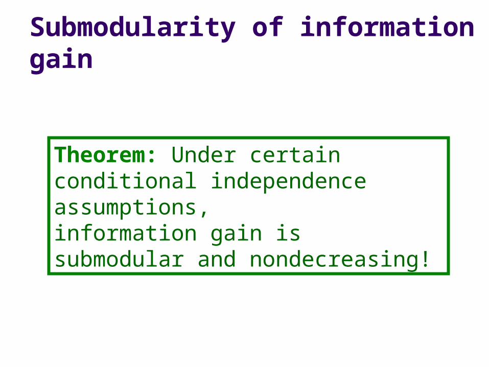
Submodularity of information gain

Theorem: Under certain conditional independence assumptions, information gain is submodular and nondecreasing!

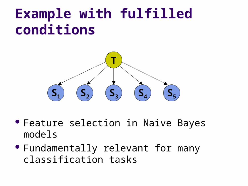
Example with fulfilled conditions

Feature selection in Naive Bayes models Fundamentally relevant for many

classification tasks

T

S5S1 S2 S4S3

Example with fulfilled conditions

T1

T2

T5T4

T3

S5

S1S2

S4

S3

General sensor selection problem Noisy sensors which are conditionally independent given

the hidden variables True for many practical problems

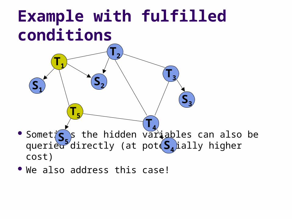
Sometimes the hidden variables can also be queried directly (at potentially higher cost)

We also address this case!

Example with fulfilled conditions

T1

T2

T5T4

T3

S5

S1S2

S4

S3

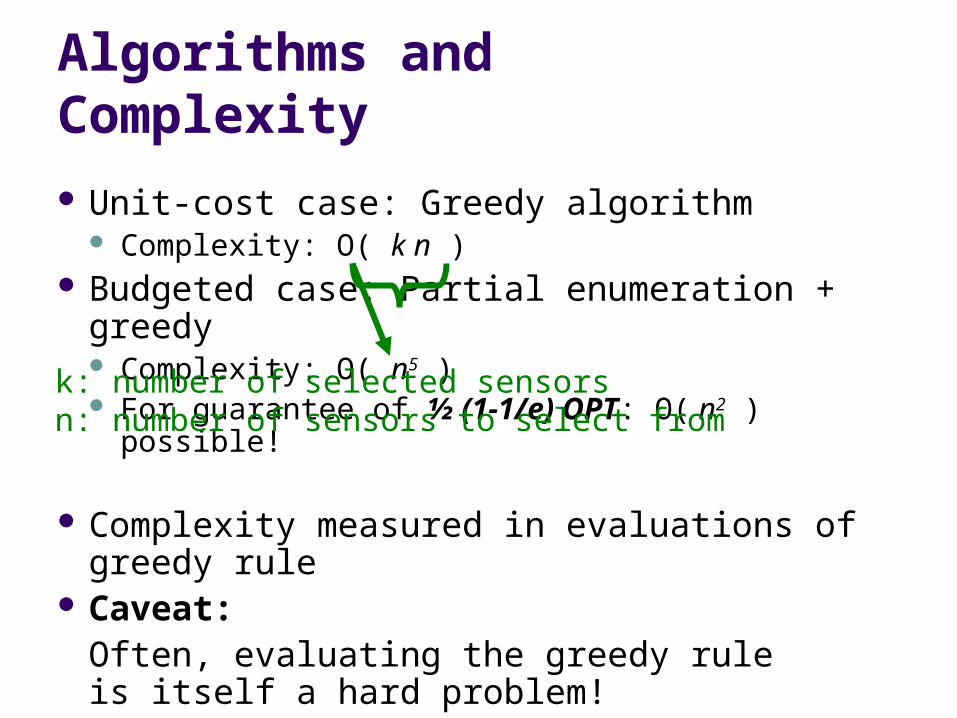
Algorithms and Complexity

Unit-cost case: Greedy algorithm Complexity: O( k n )

Budgeted case: Partial enumeration + greedy Complexity: O( n5 ) For guarantee of ½ (1-1/e) OPT: O( n2 ) possible!

Complexity measured in evaluations of greedy rule

Caveat: Often, evaluating the greedy ruleis itself a hard problem!

k: number of selected sensorsn: number of sensors to select from

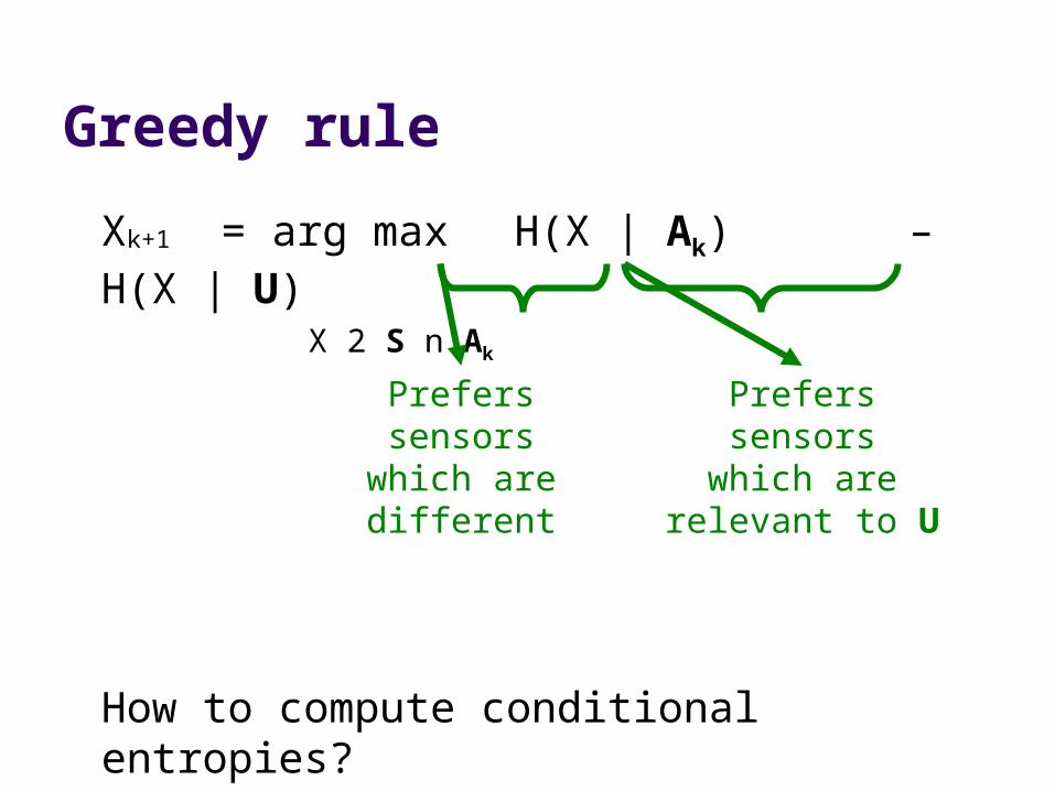
Greedy rule

Xk+1 = arg max H(X | Ak) – H(X | U) X 2 S n Ak

How to compute conditional entropies?

Preferssensors

which arerelevant to U

Preferssensors

which aredifferent

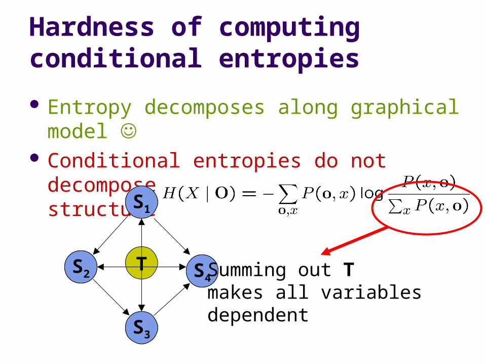
Hardness of computing conditional entropies

Entropy decomposes along graphical model Conditional entropies do not decompose along

graphical model structure

T

S1

S2 S4

S3

S1

S2 S4

S3

Summing out Tmakes all variables dependent

But how to compute the information gain?

Randomized approximation by sampling:

aj is sampled from the graphical model

H(X | aj) is computed using exact inference for particular instantiations aj

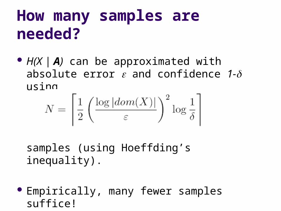
How many samples are needed?

H(X | A) can be approximated with absolute error and confidence 1- using

samples (using Hoeffding’s inequality).

Empirically, many fewer samples suffice!

Theoretical Guarantee

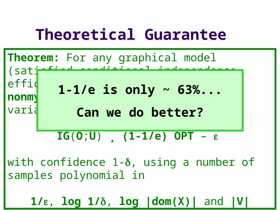
Theorem: For any graphical model (satisfied conditional independence, efficient inference), one can nonmyopically select a subset of variables O s.t.

IG(O;U) ¸ (1-1/e) OPT –

with confidence 1-, using a number of samples polynomial in

1/, log 1/, log |dom(X)| and |V|

1-1/e is only ~ 63%...

Can we do better?

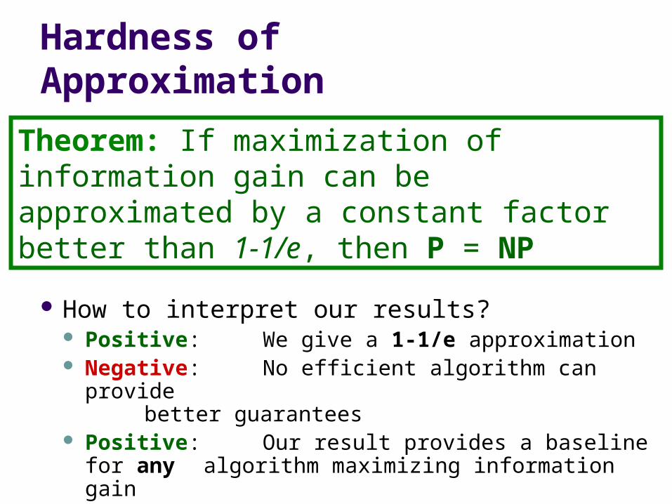
Hardness of Approximation

Proof by reduction from MAX-COVER

How to interpret our results? Positive: We give a 1-1/e approximation Negative: No efficient algorithm can provide

better guarantees Positive: Our result provides a baseline for any

algorithm maximizing information gain

Theorem: If maximization of information gain can be approximated by a constant factor better than 1-1/e, then P = NP

Baseline

In general, no algorithm will be able to provide better results than the greedy method unless P = NP

But, in special cases, we may get lucky Assume, algorithm TUAFMIG gives results

which are 10% better than the results obtained from the greedy algorithm

Then we immediately know, TUAFMIG is within 70% of optimum!

Evaluation

Two real world data sets Temperature data from sensor network

deployment Traffic data from California Bay area

Temperature prediction

SERVER

LAB

KITCHEN

COPYELEC

PHONEQUIET

STORAGE

CONFERENCE

OFFICEOFFICE50

51

52 53

54

46

48

49

47

43

45

44

42 41

3739

38 36

33

3

6

10

11

12

13 14

1516

17

19

2021

22

242526283032

31

2729

23

18

9

5

8

7

4

34

1

2

3540

52 Sensor network deployed at a research lab

Predict mean temperaturein building areas

Training data 5 days, testing 2 days

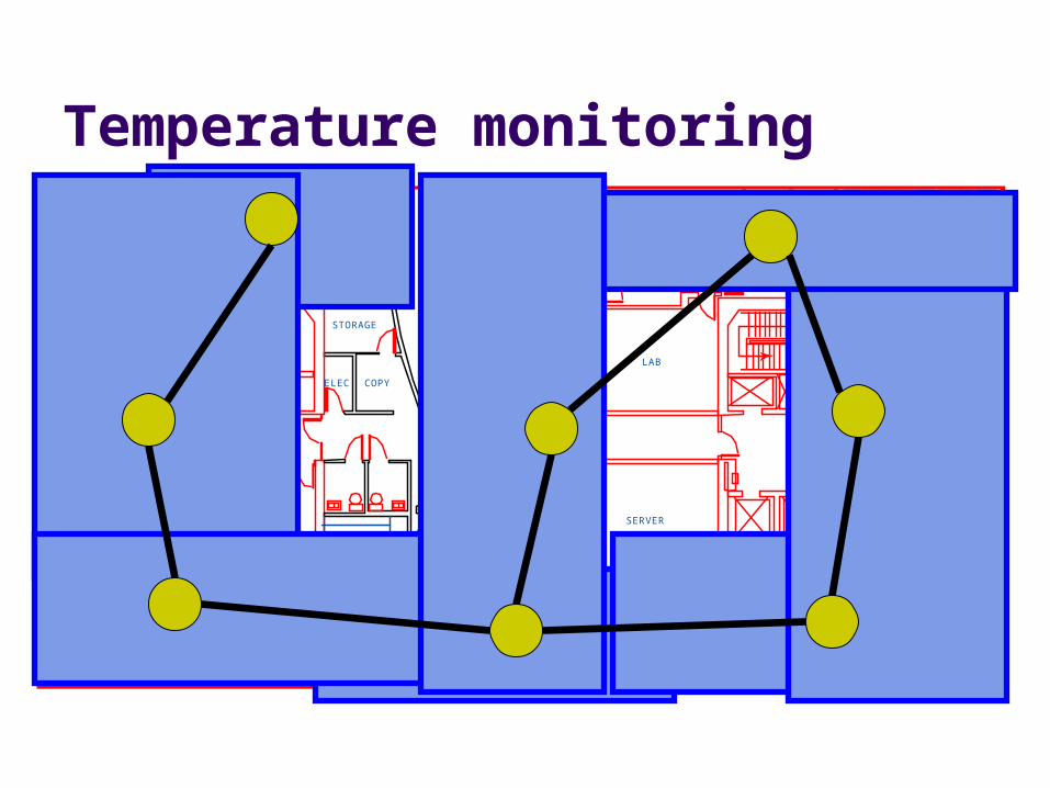
Temperature monitoring

SERVER

LAB

KITCHEN

COPYELEC

PHONEQUIET

STORAGE

CONFERENCE

OFFICEOFFICE50

51

52 53

54

46

48

49

47

43

45

44

42 41

3739

38 36

33

3

6

10

11

12

13 14

1516

17

19

2021

22

242526283032

31

2729

23

18

9

5

8

7

4

34

1

2

3540

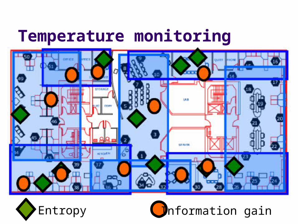
Temperature monitoring

Entropy Information gain

Temperature monitoring

Information gain provides significantly higher prediction accuracy

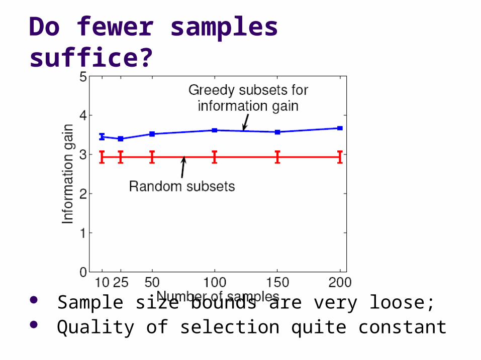
Do fewer samples suffice?

Sample size bounds are very loose; Quality of selection quite constant

Traffic monitoring

77 Detector stationsat Bay Area highways

Predict minimum speedin different areas

Training data 18 days,testing data 2 days

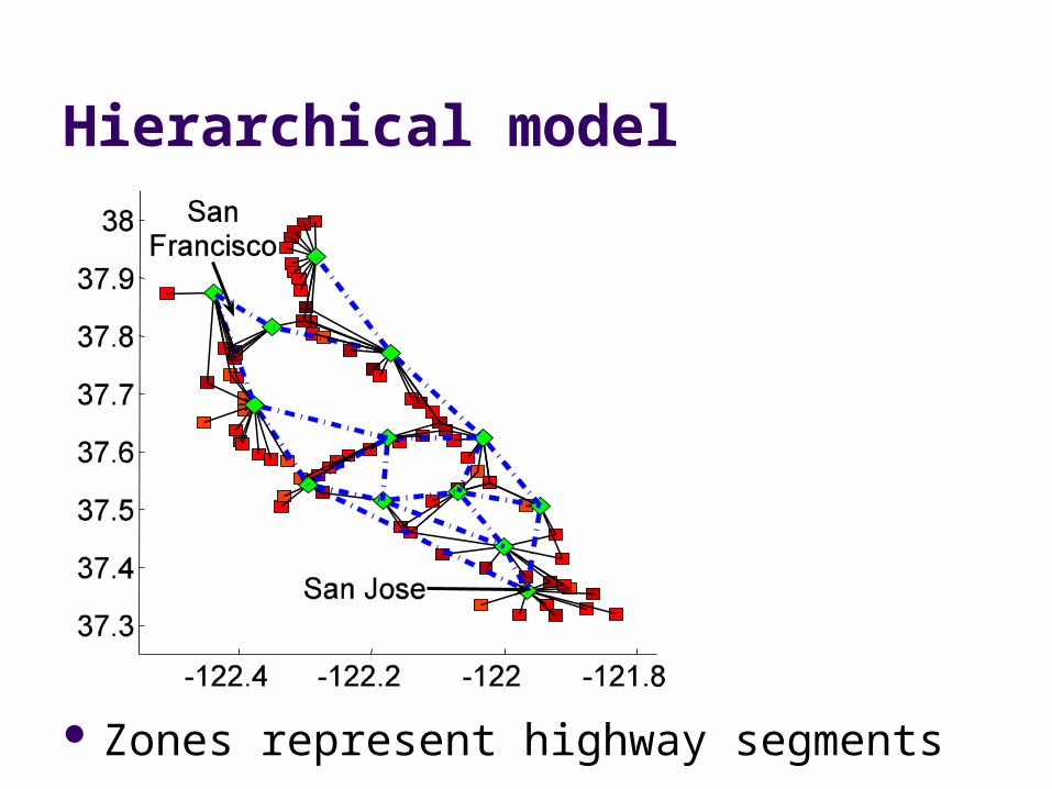
Zones represent highway segments

Hierarchical model

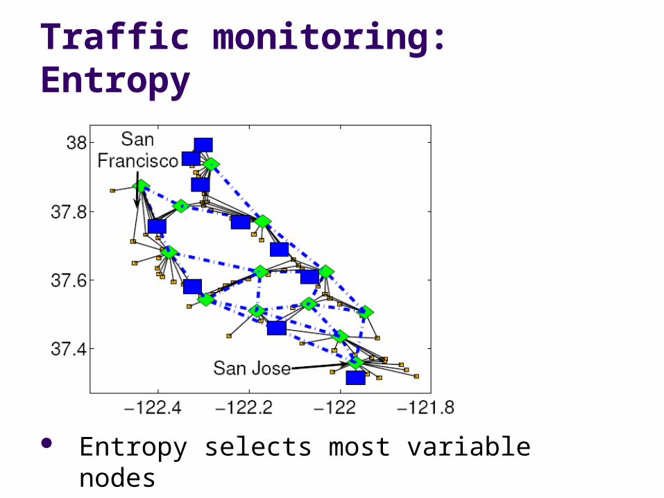
Traffic monitoring: Entropy

Entropy selects most variable nodes

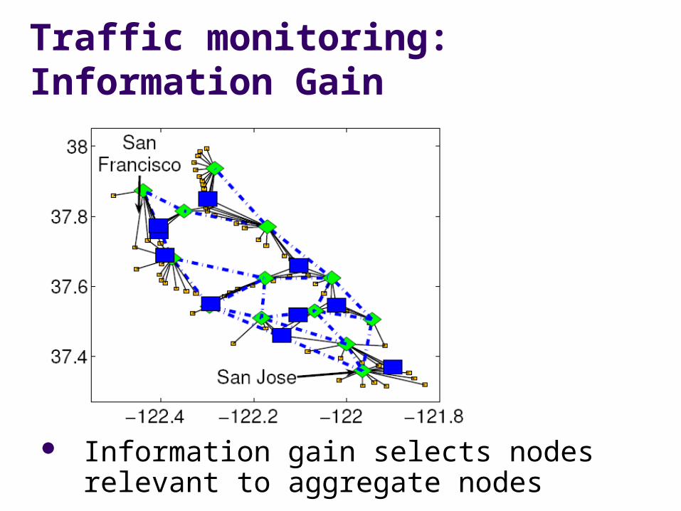
Traffic monitoring: Information Gain

Information gain selects nodes relevant to aggregate nodes

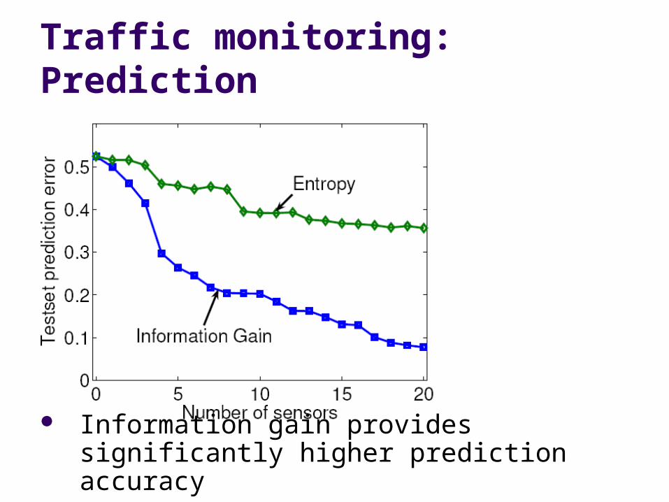
Traffic monitoring: Prediction

Information gain provides significantly higher prediction accuracy

Summary of Results

Efficient randomized algorithms for information gain with strong approximation guarantee (1-1/e) OPT for large class of graphical models

This is (more or less) the best possible guarantee unless P = NP

Methods lead to improved prediction accuracy