:

. (w

tb

#

I

I

I

1-

-- .

TECHNICAL NOTE 3764

NEAR NOISE FIELD OF A JET -ENGINE EXHAUST

H - CROSS CORRELATION OF SOUND PRESSURES

By Edmund E. Cal.laghan,Walton L. Howes, and Willard D. Coles

Lewis Flight Propulsion Laboratory

Cleveland, Ohio

-

Washington

September 1956

. .. .-. —— .. . .. .. . .. . . .. .. . . .. ------- . .. .. .. .. . . . . ----

t

,.1

(

.-- ../.-.

TBCHUBRARY KAIW, NM

“.

llnlMlulllluMIImNATIOI’?ALADVISORY COMMITTEE FoR AERONAUTIC% CICILLL71

NEAR NOISE

!CECHIU?2ALl!JOTE3764

FIELllOF A JXT-EIWJ.NEEXBAUST

II- CROSS CORRELATION OF SOUND PRESSURFrS

By Ehund E. Callaghan, Walton L. Howes, and Willard D. Coles

Aircraft structures located in the near noise field of a jet engineare subjected to extremely high fluctuating pressures that may causestructural fatigue. Studies of such structures have been limited by lackof knowledge of the loadings involved. ~ addition to the magnitude andfrequency distribution of the acoustic pressures, it is necessary to knowthe cross correlation of the pressure over the surface area. A correla-tion technique has been used to determine this statistical relation inthe near sound field of a large turbojet engine. Measurements with micro-phones were made for a range of jet velocities at locations along the jetand at a distance from the jet. Free-field correlations of the over-allsound pressure and of the sound pressure in frequency bands from 100 to1000 cps were obtained both longitudinally and laterally. In addition,correlations were obtained with microphones mounted at the surface of aplate that was large compared witlithe distance over which.a positivecorrelation existed.

The region of positive correlation was generally found to increasewith distance downstream of the engine to 6.5 nozzle-exit diameters andremain nearly constant thereafter. In general, little change in thecorrelation curves was found as a function of jet velocity or frequencyband width. The distance from unity to first zero correlation was greaterfor lateral than longitudinal correlations for the same conditions andlocations. The correlation curves obtained in free space and on the sur-face of the plate were genera12y similar.

The results are interpreted in terms of pressure loads on surfaces.

INTRODUCTION

The extremely large acoustic radiation produced by a jet-enginehaust has resulted in several serious problems. The far-field noiseannoyance difficulties are well known (refs. 1 to 4). Anotherj and

ex-

.. —------ . .. ..- .--. .— ---. — —-— —--- -— -—. — —-— -- ——————— -

.-— .— __ —.-

.

2 NAM TN 3764.

perhaps more serious, problem exists in the near noise field (refs. 5 and6). In this region} the aticral% itself is stijected to extremely highfluctuating pressures (40 lb/sq ft) that may cause structural fatigue.

Because of the importance of the structural problems createdby jetnoisej the NACA Lewis laboratory has undertaken an experimental investi-gation of the character of the sound field near the Jet of a full-scaleengine. The spectra and over-all sound pressures are reported in ref-erence 7. “

In order to calculate the stresses in a structure, it is necessaryto know not only the acoustic pressures and spectra but also the spacedistribution of the pressures. In an essentially random acoustic field,such as that produced by a jet, the distribution of pressures over a swr-face is determinedly correlation techniques. In this report, the appli-cation of correlation techniques to the determination of load distribu-tion is discussed, and the results of correlation measurements in thenear field of a full-scale turbojet engine are reported.

.

,,An electronic analog computer for determining correlation coeffi-

cients is described in the appendix by Charming C. Conger and Donald F.Berg.

Correlation measurements have been made both longitudinally andlaterally to the jet (fig. 1). The majority of the measurements weremade with the microphones in free space. A single set of data is givenwith the microphones placed in a plate of fairly large dimensions.

A

a

B

c

d

~,e

F

f

. SYMEIOL6

The following symbols are used in this report:

source strength

any fluctuating quantity

pressure amplitude of sound wave

speed of sound

nozzle-exit diamet-

voltages

force

frequency -

NACA TN 3764

K,k

P,p

R

r

e

T

t

x

xl

Y

z

a,$

u

constants

fluctuating pressures

correlation coefficient

distance from source to receiver

microphone separation

time period over which signal was integrated

time

distance

distance

Vertical

along jet centerline from nozzle exit (fig. 1)

along jet boundary from nozzle exit (fig. 1)

distance from jet centerline (fig. 1)

horizontal distance

phase angles

angular frequency

Subscripts:

o output

x longitudinal

from jet centerline (fig. 1) “

xl longitudinal along jet boundary

Y lateral

1,2 position or time

SCUND-I?RESSURE

The characteristics of any noise

CORRELATION

field are usually given in terms ofits time-averaged, that is, statistical, properties such as over-alJ.sound-pressure levels and spectra. These properties are determinedlymeasuring the root-mean-square pressures over the whole frequency rangeand in frequency bands. The sound pressures createdby a jet are random,,in time, but their time-averaged products may have a spatial relation.,

. ..— —.- -_ .-. — — .— ——-. -.— .——. — . —.—_.—_—

4 I?ACATN 3764

The usual properties of root-mean-square pressure and spectra may not besufficient to define the load on a structure. The loading on a surfaceis related not only to the root-mean-square pressure at various points,but also to the degree of unison of the pressures acting over the surface.E the pressures at all points are in unison, then the root-mean-squareload is simply the product of the root-mean-square pressure and the areaof the surface. Usuallyj however, the instantaneous pressures are not inunison and the relation between the pressures is measured in terms of astatistical relation such as a correlation coefficient.

The correlation coefficient R of any two fluctuating quantitiesa is defined as

-. ‘=4%IZ?wh=e the bars indicate a time average so that

●

al% = ~l+ti=

where, for practical purposes, T

1z J al(t)%(t) dt

o“

is a time of much longer duration thanthe p~iod of the lowest-tiequency involved. For the case of fluctuatingpressures,

i..

where P1 and ~ are the instantaneous fluctuating pressure at two

points.

The value of R is therefore determined by measuring the instan-taneous pressures ~ and ~ with two microphones, obtaining theti

time-averaged product, and normalizing with the product of the root-mean-squere values of the two pressures. In the special case where the ~es-sures ~ and P2 are linearly related (act in unison), then ~ = k%

and R=l. Jf ~ is completely unrelated to PI} the product 31P2

has equal probability of being positive or negative and, consequently,the time average of the product will be Z=O. Therefore; zero correla-tion is obtained when the relation between ~ and ~ is completely

,-

random. There are} however, other conditions that yield zero correlation.,’

——. . .—---

o(33o-#

NACATN 3764

The casesimple source

5

of the sound pressures generated by a single-frequency u)of strength A can be considered. H rl and r2 are

the respective distances of the microphones from the source,the following sketch,

Microphone 1

vu Microphone 2

/I[

/0

0

the pressures at

The pressures ata= u(r2 - rl)/c

averaged product

I /’/&--- Simple

1 and 2 are given as

source strength A

%=Acoso’trl

P2=$ cos(ah -f-a)

as shown in

1 and 2 are out of phase by =wgle a} whereand c is the speed of sound in the medium. The

~ is

JT

1 A2 A2

~= 1~ ~ — Cos at Cos(mt + a)dt =—cosaTam ~ ‘1r2

2rlr2

and

--- —.——.— -———

6 NACA TN 3764

Therefore, the correlation coefficient R between 1 and 2 is cos a. ““For a single frequency the correlation coefficient and the cosine of thephase angle are equivalent and, hence, can have any value from -1 to 1.There is no real necessity for limiting the previous example to a singlesource. Any nuniberof sources that ~oduce sinusoidal waves of a singlefrequency and random strength wiXL induce resulting pressure fluctuations

pl=%cos~

and

% = B2 COS (d + ~)

at the two microphones. The coefficients B re~esent the resultingpressure amplitudes at the microphones, and ~ is a resultant phaseangle. The correlation coefficient is then

.

where

@ = tan-l

U? ~ is 90°) thenpressures at 1 and 2

R = Cos p

(

Alsin~+A2sin~+. ..~ sin%

A1-cos~+~cos ~+... &COS=$

R=O. Furthermore, it can be shown that, if thewere of two different frequencies, the correlation—

would always be zero. ,

It should be evident that, even M the sound pressures are distrib-uted over a wide frequency range, the pressure correlation between twopoints results only from the relation between the identical frequencycomponents at the two points.

If a series of correlations are determined by roving one microphonerelative to another, a graph such as shown in figure 2(a) may be obtained.When the microphones are very close togetha?j the two microphones measurethe same pressure and the correlation is unity. As the microphones areseparated, the correlation coefficient fa13.sbelow unity. A usefulequivalent to the load on a rigid surface can be determhed from thecorrelation coefficient in the following manner: From the definition ofthe correlation coefficient, it follows that

R

where all quantities on the right side of the equation are obtainable.

@

,,

.—. . -.. — . —— — .——.

lWCA TN 3764 7

The time-averaged quantity ~ is a constant for any given microphone

separation. Thus, over the total period T the constant value of ~

is equivalent to the product P1P2 of two steady-state pressures pl and

P2. If a value is selected for Pl) which maybe regarded as the pressure

associated with the stationary microphone, then P2 can be computed mom

where, by virtue of R, P2 is a function of the microphone separation.

Because R = 1 when the microphone separation is Zero, P1 = r $ and

p2=@=~. _When the microphones are separated, Pl = r p?, as be-

fore, but P2 = R VP22 where P2 is the most probable value of ~=

corresponding to 6pl = 2. The last four equations permit computation

of a time-average pressure distribution along a line connecting themicrophones when the sound pressure at the statio~ microphone is

rPI = p!. The result amounts to replacing the “randompressure distribu-

tion along the line of microphone separation by an equivalent steady-state distribution, as sho,yn-tnfigure 2(a).

In order to obtain a measure of the force distribution OV- a sur-face area, it is necessary to measure correlations in both the lateraland longitudinal directions=(y- and x-directions, respectively, fig. 1).Worn such measurements, the area distribution of the pressures can beapproximated in the manner shown in figure 2(b). In this figure, curvesof constant P2 have been assumed to be ellipses in planes parallel to

the x,y-plane. By using such a distribution, it is possible to calcu-late an effective instantaneousforce distribution on the plate. Beforesuch a concept has any value, however, it must be associated with somefrequency; that is, the pressure variation with time must be lmown.

The fluctuating pressure field near a jet is of an extremely complexcharacter since, at any point in the field, the pressure results from aspace distribution of randomly fluctuating sources. l?urth~re, eachsource produces a fairly wide range of frequencies (ref. 7). However,the wave form of the sound at any point results from the cumulative ef-fect of all the sources. The usual wave form in the near field of a jethas a random amplitude and a fairly peaked frequency distribution.Hence, the largest contribution to the over-all sound-pressure correla-tion will result from the energy centered around this peak. To a first

. ---- . ——.. — .— --- .— - —. ——— ——— —---— .—.. -

8 IWCA TM 3764

approximation, therefore, the loading distribution of the over-all pres-sures previously described might be assumed to fluctuate harmonicallywith a frequency corresponding to the peak frequency of the spectrum.

Surfaces in aircraft are usually resonant and would normallybe ex-pected to fail most rapidly if excitedby pressure fluctuations in theband of resonant frequencies. Thus, the pressure correlations of inter-est in many cases are those associated with a narrow band of frequencies.The data reported herein have, therefore, been analyzed in approximatelyl/2-octave bands. In oral- to check the l/2-octave analyses, the correla-tion coefficient was also determined for a narrow band width (12 CPS) witha midf’requencyof 500 cps.

In order to determine the fatigue of a resonant panel, the panelshould be loaded with a harmonically fluctuating load corresponding tothe resonant frequency band. The amplitude of the load over the surfacewould be determined from the correlation curve for the band of tnterestand the root-mean-square pressure (h the same band). The procedurewould.be the same as described previously for over-all sound pressuresbut limited to the band width for which the plate is resonant.

The practical determination of the correlation coefficient for thisinvestigationwas obtained by the following method: The output voltage

. e of a microphone is linearly related to the fluctuating pressures forthe.range of frequencies and ~essures of interest; so

P1 = klel

4and

p2 = k2e2

and, therefore,

The

space iscorrelation coefficient of sound pressures attherefore obtained in exactly the same manner

two points inas the correlation

coefficient for two fluctuating velocities in turbulence measurements

.

1?CDo

.

(refs. 8and 9]. It is therefore possible to obtain correlation coeffi-cients quite simply with a correlation computer of the type used in ref-erence 9 and describ~ in detail in the appendix of this report.

.1

.

●

NACA TN 3764

. APPARAms AND PROCEDURE

The equipment required for the determination

9

of the space correla-tion of the acoustic pressures near the Jet can best be described inthree parts: (1) the engine and its associated equipment, (2) the equip-ment for obtaining and recording the acoustical data, and (3) the correla-tion equipment. The first two iteny and their use willbe described inthe succeeding paragraphs together with a partial description of the cor-relation equipmentthe appendix.

and its use. The correlation computer is described in

Engine

The engine used for the investigation was a large axial-flow turbo-jet of approximately 10jOOO-pound-thrustrating. The exhaust nozzle was

2% inches in diameter. The pressure ratio across the nozzle under test-

stand conditions when the engine was operated near rated power wasapproximately 2.’2,resulting in choked flow at the nozzle and expansionto slightly supersonic flow just downstream of the nozzle. The enginewas mounted in the outdoor thrust stand shown in figure 3. Engineoperating conditions were chosen that would allow duplication of the en-gine thrust condition over the range of atmospheric conditions expectedto prevail during the experiments. In addition, the time required to ob-tain the correlation data limited the engine operation to somewhat lessthan ftillpower. All the data presented herein, unless otherwise indi-cated, were obtained at a thrust of approximately 9600 pounds and a jetvelocity (ratio of thrust to mass flow) of 1850 feet per second. Theengine was equipped with an afterburn=, but it was not used for thisinvestigation.

The engine and thrust stand were located so that no lsrge sound-reflecting surfaces other than the ground were near the jet in any direc-tion downstream.of the engine. The engine centerline was 6 feet aboveground level.

Temperature and total-pressure (velocity) surveys were made at sev-eral locations along the jet as far downstream as approximately 40 feetfrom the engine. Flromthese surveys, the limits of the thermal and ve-locity boundaries (temperature and total pressure equal to anibient)weredetermined for conditions of little or no wind. Measuring stations werethen set up outside the jet boundaries as shown in figure 1. These pre-cautions were necessary to allow the acoustic data to be obtained as closeto the jet as possible without subjecting the microphones to undue tem-perature and jet-velocity effects.

10 NACA TM 3764

. Acoustical Equipment .

In order to obtain the space correlation data, it was necessary toprovide a means for simultaneouslyrecording the signals from two micro- ‘phones that could be precisely located in the sound field.

Microphone positioning. - A remotely controlled and remotely indi-cating microphone-positioningdevice was used to provide the microphonemovement req@md. One of the microphones was mounted in a fixed positionto the bo~ of the device and the other was mounted on a movable carriage.The whole assdly could be positioned at aq point in the sound fieldoutside the jet. Positioning of the fixed microphone and the traversingmechanism was accomplished by measurement from p~ ent markers. Aphotograph of the positioning device in placestations behind the engine is shown in figuregation the positioner was motified to providedirection.

At the beginning of each experiment, thezontal and adjacent with the microphone faces

at one of the measuring4. I@er in the investi-motion in the vertical

two microphones were hori-in the same vertical plane ‘

and at the engine centerline hei@t. For the correlation data t&en alongthe jet boundary (xl-direction),this vertical plane, the a,b,c,d-plane in ,

figure 1, was along the microphone location line. Correlation data werealso obtained at three locations away from the jet boundary with the planeof the microphone faces parallel to the jet centerline (x-direction)andin the e,f,g,h-plane. For the longitudinal correlations, one microphonewas moved in a horizontal direction away from the fixed microphone andtoward the engine. For the lateral correlations, the microphone wasmoved upward from the engine centerline height.

With the microphones adjacent, the microphone centers were approxi-mately 1 inch apart. Magnetic tape records of several minutes durationwere made with the microphones adjacent for purposes of calibration ofthe correlation computer. The microphones wme then separated in smallincrements and tape records of approx~tely l-minute duration were takenat each position. Small increments were taken at first, and then largerincrements w~e used when the total separation was sev~al feet.

For the study of the longitudinal correlation over the surface of apanel, a stiff aluminum plate consisting of three segments was used asshown in figure 5. The center segment was a sliding bar approximatelytwice the length of the fixed top and bottom sections. me ~crophoneswere mounted behind porous, sintered stainless-steel plugs flush with theplate surface to protect the microphones. These plugs do not affect soundWessures for the range of frequencies of interest. The movable micro- .

phone was mounted near the center of the bar and the fixed microphone inthe adjacent plate. The actuating and position-indicatingmechanism was 1

NACA TN 3764 11

)III

I

II

similar to that previously described. The plate was mounted on verticalstands at the engine centerline height. The face of the plate was in avertical plane along the microphone location line near the jet boundary.

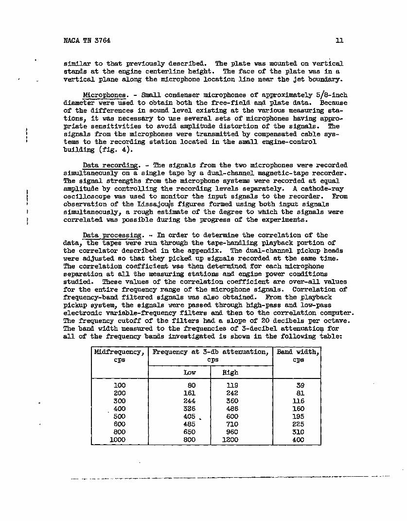
Microphones. - Small condenser microphones of approximately 5/8-inchdiameter were used to obtain both the free-field SJ.@plate data. Becauseof the differences in sound level existing at the various measuring sta-tions, it was necessary to use several sets of microphones having appro-priate sensitivities to avoid amplitude distortion of the signals. Thesignals from the microphones were transmitted by compensated cable sys-tems to the recording station located in the small engine-controlbuilding (fig. 4).

Data recording. - The signals from the two microphones were recordedsimultaneously on a shgle tape by a dual-channel magnetic-tape recorder.The signal strengths from the microphone systems were recorded at equalamplitude by controlling the recording levels separately. A cathode-rayoscilloscope was used to monitor the input signals to the recorder. I!romobservation of the Lissajo@ figures formed using both input signalssimultaneously, a rough estimate of the degree to which the signals werecorrelated was possible during the progress of the experiments.

Data processing. - In order to determine the correlation of thedata, the tapes were run through the tape-handling playback portion ofthe correlator described in the appendix. The dual-channel pickup headswere adjusted so that they picked up signals recorded at the same time.The correlation coefficient was then determined for each microphoneseparation at all the measuring stations and engine power conditionsstudied. These values of the correlation coefficient are over-all valuesfor the entire frequency range of the microphone signals. Correlation offrequency-band filt=ed signals was also obtained. lhomthe playbackpickup system, the signals were passed through high-pass and low-passelectronic variable-frequency filters and then to the correlation computer.The frequency cutoff of the filters had a slope of 20 decibels per octave.The band width measured to the frequencies of 3-decibel attenuation forall of the frequency ‘bandsinvestigated is shown in the folloting table:

1!lMfrequency, Frequency at 3-db attenuation, Band width,Cps Cps Cps

Low High I

100 80 119 39I

200 161 242 81300 244 360 116

. 400 326 486 160500 405 ● 600 195600 485 710 225800 650 960 3101000 800 1200 400

— ..- -. - — -. .--— —-—-- —---— —--— —-— — -—.-— .— -——— --- . -—-

12 IiACATN 3764

In addition, one set of narrow-band filters was made that had a band- ‘pass width of 12 cps at the 3-decibel attenuation point for a mid-frequency of 500 cps. .

The limitation of the frequency bands shown (100 to 1000 CPS) in thepreceding table results from the frequency distribution of the sound andthe limit on the maximum pmsible signal (voltage) level that can be im-pressed on the tape. The peak of the frequency spectrum occurs between100 and 1000 cps for all the acoustical near field (ref. 7). For mostpositions the spectrum peak occurs near 500 CPS. The available signalin each band drops off quite sharply on either side of’the spectrum peak,and for most cases bands above 1000 and below 100 CPS do not contain asufficient signal for a reasonably accurate value of correlation withthe computer described in the appendix. This, however, should not beparticularly important since the sound pressures outside the 100- to1OOO-CPS region are far below the peak values (ref. 7) and probablywould not have sufficient energy to affect the aircraft structure.

It would, of course, be possible to filter the microphone signal in ..frequency bands ahead of the recwder and, hence, obtain data over a muchwider frequency range. This would result in an exceedingly large amountof engine operation time and, therefore, was not considered.

\ RESULTS AND DISCUSSION

The results presented herein are largely confined to the effect ofvarious parameters, such as jet velocity and measurement position, on thecorrelation coefficient. All the correlation figures presented havecorrelation coefficient as an ordinate and a dimensionless microphoneseparation (ratio of microphone separation to nozzle-exit diam. s/d)as the abscissa. The data presented wqre obtained both longitudinally(x-or xl-direction) and laterally (y-direction). The xl-direction 3-s

measured along the jet boundary and is at an angle of 9.8° to the x- oraxial direction (fig. 1).

Longitudinal Correlation

A t~ical set of correlation data is shown in figure 6. These datawere obtain~ at a position approximately 17.3 nozzle-exit diametersdownstream (measured along the jet boundsry) of the engine and 12.1nozzle-exit diameters from the jet centerline. Correlations are shownfor the over-all sound pressure and for sound pressures in various fre-quency bands with midfrequencies from 100 to 1000 CPS. The width of each “ ‘“band and its midfrequency is tabulated in the APPARATUS AND PRWEDUREsection. i

—.

NACA TN 3764 13 “

‘oalCJ

The correlation curves of figure 6 show interesting characteristics.There is a definite order to the results. The higher midfrequencies showa decreased region of positive initial correlation. The microphoneseparation for which the correlation coefficient is initially zero occursat decreasing s/d values, and the curves sharply steepen with increasein frequency. The maximum negative correlation and the second zero-correlation points follow this same trend. Decreasing frequency resultsin a movement of both the maximum negative and the second zero correlationtoward larger values of s/d. The maximum negative correlations show adefinite tendency to increase (negatively)to a midfrequency of 400 CPSand to decrease thereafter.

For the data shown in figure 6, the peak of the frequency spectrumoccurs between 300 and 400 CPS. The over-all correlation curve also fallsbetween the 300- and 400-cPs midfrequency correlation curves. All thecorrelation data exhibited this characteristic; that is, the over-all cor-relation curve fell near the correlation curves corresponding to the peakof the spectrum. The approximation of the over-all curve by a curve ofsingle frequency as described previously in the section SOUND PRESSURECORRELATION would appear to be useful for structural loading purposes.

Effect of jet velocity. - The over-all sound-pressure correlationfor a range of jet velocities from 630 to 1780 feet per second is shownin figure 7. These data were obtained along the jet boundary 2.16nozzle-exit diameters downstream of the nozzle exit. In general, theshapes of the curves axe nearly the same, and the effect of jet velocityappears to be quite small.

The small effect of velocity might well be inferred from the resultsof reference 9, which show very little effect of exit velocity on thescale and intensity of turbulence. Since the relation of the sound-pressure spectrum nesr the jet is quite similar to the turbulent ve-locity spectrum in the jet (ref. 7), it wouldbe expected that the near-field sound would reflect the same trends as the turbulence results.

The effect of velocity on the correlation coefficient for severaltiequency band widths is shown in figure 8. As might be expected fromthe previously discussed results on the over-all sound-pressure correla-tion, the effect of velocity on the correlation for the various band widthsis quite small.

Effect of position. - The correlation of the over-all sound pressuresat various positions along the jet boundary is shown in figure 9. Nearthe nozzle exit, 2.16 nozzle-exit diameters downstream along the boundary,the region of positive correlation extends to an s/d value of 0.385.Farther downstream the region of positive correlation increases, but at6.5, 10.8, and 17.3 nozzle-exit diametem the region of positive correktion is neerly the same and appears to give a first zero crossing atabout s/d of 0.93. The correlation of these same data for the various

14 NACA TN 3764

frequency bands is shown in figure 10. b general, the correlations of.

figure 10 follow the general trend of decreasing region of positive cor-relation with increasing frequency, as discussed previously (fig. 6).This is shown quite clearly in figure Xl, where the initial zero-crossing

u

point (fig. 10) is plotted as a function of frequency. The straight linerelation of the data indicates that the distance for ~tial zero crossingis related to the frequency

The value of n appears tothe nozzle to about 1.2 far

by an equation of the form

kSjd =

(frequency)n

increase nonuniformly from about 0.5 neardownstream.

*oCao

The results shown in figure 10, however, do not show exactly thesame order as the correlations of over-all sound pressures in figure 9.This should be e~ected since the spectrum distribution of the soundchanges in moving downstream from the nozzle exit. The peak of the sound-pressure spectrum curve occurs at decreasing frequency with increasing

?

downstream distance (ref. 7). )3?space and time are relatedby an eddyconvective velocity or the speed of sound, the correlation of the over-allsound pressures can be achieved from the Fourier transform of the sound-pressure spectrum. It shouldbe expected, therefore, that the shfit inthe spectrum would showup in the band-pass correlations.

In figure 12 is shown a comparison of over-all sound-pressure cor-relations measured on the jet boundary and 12.1 nozzle-exit diametersfrom the set centerline for two downstream distances. At a downstreamdistance of 6.5 nozzle-exit diameters, the shape of the correlationcurves are vastly different. On the boundary, the first zero-correlationposition occurs at an s/d value near 0.85, whereas 12.1 nozzle-exitdiameters from the jet the correlation coefficient appeers to approachzero asymptotically. At 17.3 nozzle-exit diameters downstream of thenozzle exit, the curves are somewhat similar, although the microphoneseparation at the ftist zero crossing is slightly larger near the jet.The data of figure 12 in the various bands are also shown in figures 6and 10 except for the position 6.5 nozzle-exit diameters downstream ofthe nozzle exit and 12.1 nozzle-exit diameters from the centerline.These correlations are presented in figure 13.

Effect of band width. - The correlation of sound pressures wouldidea13.ybe made for a band width corresponding to the band width to whichthe surface is responsive. This would not necessarily be worthwhile, asillustrated in figure 14. In this figure, data at several locations inthe field are presented for two band widths, 195 and 12 cps, both havingessentially the same midfrequency (500 CPS). It is evident that theinitial region of positive correlation is practically independent of the

.— -—...

NACA TN 3764 15

,..

.

width of the band pass for a band pass less than 1 octave. There is atendency when reducing the band width for an increase in the maximumnegative value of the correlation coefficient but little effect on thepositions wh=e the values of first zero crossing occur. The small ef-fect of decreasing the band width from 195 to 12 CPS indicates thatfurther decreases in the band-pass width would show only an increase inthe absolute magnitude of the second maximum positive and negative valuesbut little change in the zero-crossing positions. This result agreeswith a similar treatment of turbulence data (ref. 9). It should beobvious that increasing the band width by an appreciable amount is boundto shift the curves toward the over-all sound-~essure correlation.

Comparison of free field and plate. - The results ~esented thus fsr“have been concerned with the correlation in free field. A point of con-siderable interest is the relation between a free-field co~elation anda correlation on a surface. It might be expected that the introductionof a surface into a sound field would cause some change in thecorrelation.

As a Weliminary estimate of this effect, a single set of data wasobtained of the correlation on a flat plate. The dimensions of the plateand the microphone locations are shown in figure 5. The data were ob-tained with the fixed microphone located approximately 2.7 nozzle-exitdiametms downstream of the nozzle exit, the long dimension of the platealong the Jet boundary, and with the plate surface tangent to the Jet.Zkom figure 9 it canbe seen that the.free-field over-all sound-pressurecorrelation is much smaller than the physical dimensions of the plate;that is, the correlation has become nearly zwo in the first 0.9 nozzle-exit diameters compared with the plate length of 1.98 nozzle-exitdiameters.

The over-all sound-pressure correlation coefficient for both theplate and free field at approximately the same spatial location is shownin figure 15. Also shown in the figure are the results for several fre-quency bands. I!romthese data it canbe seen that the surface correla-tion and the free-field correlation for each frequency ae not too dif-ferent. The correlation curves for the plate have slightly differentshapes and greater negative values than the free-field results. Thismight well be causedby the slightly different locations of the plateand free-space measurements. The plate location (fixed microphone) wasap~oximately 1 foot downstream of the free-field measurements. It wm.ildappear, therefore, that correlation is relatively unaffected by thepresence of the body in the field, at least for the case where the bodyis larger than the area over which.the pressures are correlated to a

. large degree.

It is interesting to note that the actual sound-pressure levels onthe plate (when placed along the Jet boundary) are much higher than thosemeasured in the free field (ref. 7).

— . . . .. . — ———-- - —--———-- — — — -- -—..— . . ..-—— —— -- — —-

16

IAeral Correlation

NACA TN 3764

In general, it would be expected that a suund-pressure correlation dwould involve a spatial volume. That is, a constant value of the corre-lation coefficientwould have a shape in space in the same sense that aturbulence correlation has in a jet (ref. 9). For structural considera- ~tions, it is necessery to know the correlation in the plane of the sur-face under consideration. Measurements have therefore been made along avertical line (y-tiection, fig. 1) at several positions corresponding tomeasurement points of longitudinal correlation. No measurements weremade in the direction normal to the plane of the longitudinal and lateralcorrelations.

Effect of position. - Correlations of the over-all sound pressuresat three positions are shown in figure 16. h each case the fixedmicrophone was held in the horizontal plane of the jet centerline (fig.1) and the movable microphone was moved vertically upward.

It is apparent fiomthe figure that the pressures are correlatedover a considerable distance. In fact, only the data at 2.16 nozzle-exitdiameters downstream along the jet boundary show a zero correlation withinthe actuator limits. H the data of figure 16 are compared with thelongitudinal correlations for the two comparable space positions (fig. 9),it is apparent that the lateral distance to the first zero crossing islarger than the longitudinal.

A single set of measurements moving the microphone vertically down-ward were made at 2.16 nozzle-exit diameters downstream along the jetboundsry. These data were nearly identical to the results obtained whenmoving the microphone upward.

Correlation in frequency bands. - The correlation in frequency bandsat 17.3 nozzle-exit diameters downstream is shown in figure 17. Thesedata show exactly the same trends as the longitudinal correlations Infrequency bands (fig. 6).

Effect of bandwidth. - The effect of band-pass width on the correla-tion for two frequency bands at two downstream distances is shown in fig-ure 18. It is appsrent that the effect of band-pass width is quite smallin the initial positive region. The maximum negative value ?.sgreater forthe smaller pass band, which agrees with the effect on longitudinal cor-relations presented in figure 14.

As part of the studyspace correlations of thelowing results obtained:

.

1SUVMARY OF RFSULTS

of the near noise field of a jet exhaust, the 4sound pressures have been measured and the fol-

NACATN 3764 17

..

.

1. The size of the region of positive longitudinal correlation ofthe over-all pressures along the jet boundary (the distance to the firstzero crossing of the correlation curves) varied from 0.385 to 0.93 nozzle-exit diameters.

2. Longitudinal correlation curves obtained over a range of jetvelocities from 630 to 1730 feet per second showed, in general, littlechange in the over-all and frequency band-width correlations as a func-tion of jet velocity.

3. F& longitudinal correlations along the jet boundary the firstzero-crossing distance was found to increase with distance from the en-gine up to about 6.5 nozzle-exit diameters. However, at distances of6.5, 10.8, and 17.3 nozzle-exit diameters downstream from the engine,there was little difference in the first zero crossing distance.

4. Longitudinal correlations measured 12.1 nozzle-exit diametersfrom the jet centerline at a distance downstream of 6.5 nozzle-exit diame-ters from the nozzle exit approached z-o asymptotically. Farther down-stream from the exit (17.3 nozzle-exit diam), the correlation curvesmeasured 12.1 nozzle-exit diameters from the jet centerline were morenearly like those at the jet boundary.

5. A comparison of the correlation curves obtained at a midflrequencyof 500 cps for band widths of 12 and 195 CPS showed small effect of bandwidth. The narrow band resulted in increases in the second maximums andminimums, but no significant change occurred in the”zero-correlationdistance.

6. Correlation curves obtained in free field and on the surface ofa plate showed only minor dissimilarity.

7. The distance over which the correlation coefficients were posi-tive was greater for lateral than for longitudinal correlations.

-Lewis Flight Propulsion LaboratoryNational Advisory Committee for Aeronautics

Cleveland, Ohio, &y 25, 1956

.

.

- -.-—- .-—-- — —— .——.. —.— —— .-— .— - — -—-— - .

NACA TN 3764

APPENDIX -

By Charming C.

The correlation computeranalog methods an equation of

CORRELATION COMPUTER

Conger and Donald F. Berg “

is a device that is designed to solve bythe form .

rT%=$ I ea(t)eb (t)dt

Jo

where T is real time, ~ is the output

ea and ~ sre the input voltages. The

be written as

fT

— 11

(1)CDo

voltage from the computer, and

correlation of two voltages may

‘= J“iJo ‘a%‘t (2) ‘

where the bsx indicates the true time average. Therefore, if K is

‘e ‘q@ ‘0 l/@~ ‘hen ‘o”= ‘o m ‘b(t)= ‘a(t + ‘t), ‘hwe ‘tis a time delay, then R is termed the autocorrelation coefficient ofea.

The operation of the computer will be described with reference tofigure 19. The two signals whose correlation is to be measured arerecorded on a dual-channel tape recorder on l/4-inch magnetic tape. Thesignalz me recorded in periods of from 1 to 30 minutes fo~owed by 10-second intervals during which nothing is recorded on the tape. All tape-recording eqpipment is commercially available and of inzlzmnnentquality.

The magnetic tape is played back on a tape handler similar to theone used in recording hut with a special playback head sx’rangement. Theplayback heads “sremounted so that one of the two heads may be translatedalong the tape with respect to the other. The smount of translation ismeasured by a micrometer head uzed to drive the movable playback head.The maximum head motion is 3/4 inch, and this motion may be measured toan accuracy of 1X1CF4 inch by means of a vernier on the micrometer head.The tape speed used on playback is 15 inches per second. Therefore, theadjustment allows an adjustable delay of from O to 50 milliseconds tohe introduced between the signals from the two playback heads. This *

adjustable delay is used in the determination of autocorrelation functionsas described previously. For cross correlations (as from two microphones), ,the delay is adjusted to zero.

— . .

.

NACA

back

TN 3764

The compensationheads. The gain

amplifiers receivecharacteristics of

19

the two signals from the pl.ay-these amplifiers have been ad- “

justed by means of passive filters to compensate for the frequencycharacteristics of the recording system. They also serve to correct forthe frequency response of the playback heads andto amplify the signalsto a level suitable for use by the remainder of the circuitry. From thecompensating amplifiers, the signals go to the variable-gain aqilifiers,as shown in the block diagram. The adjustable-gainfeature of theseamplifiers is usedto set the scaling coefficient K of equation (l).

The switching circuit (indicatedin fig. 19) is usedto switch theoutput volteges of the variable-gain amplMiers to a monitoring oscillo-scope, a vacuum-ttie voltmeter, or the electronic multiplier. Theswitching cticuit aids in setting up the computer and in checking itsoperations during use.

Ihwm the switching circuit, the two signals are applied to theelectronic multiplier. The multiplier produces an output voltage pro-portional to the instantaneousproduct of the input voltages. The productvoltage is applied to resistance-capacitanceaveraging circuit of con-ventional design. The average amplitude of the product voltage is thenread from the vacuum-taibevoltmeter.

When used for atiocorrebtion measurements, the computer is usuaXlyadjusted so that the correlation maybe read directly from the voltmeter.The adjustment consists of the fo~owing: The heads are adjusted untilzero time lag is produced; therefore, the correlation is unity. Then,the gain of the variable-gain amplifiers is adjusted until the output ofthe multiplier indicates 1 volt full scale on the voltmeter. With thisinitial setting, the autocmrelation coefficient maybe read directlyfrom the voltmeter dial as a function of the time delay obtainedbyadjusting the movable head.

.

Two blocks of figure 19 remain to be described, the calibrationcircuit and the tape-reversal control. The calibration circuit providesappropriate alternating-currentand direct-current voltages that maybeswitched into the electronic multiplier. These voltages are used forcalibration and adjustment of the multiplier prior to use.

The tape-reversal control is usedto operate automatically the tapehandler. The control uses the 10-second blank intervals at the end andbeginning of a section of recodded data on the tape to stop automatically,rewind, and restart the tape handler. Use of the controller, therefore,allows a section of the tape to be played back repeatedly without atten-tion from the operator and produces the effect of a loop of tape withoutthe necessity of cutting and splicing the tape.

. . ..-. .. —.- . .—. — .- —.. — -— —- .—— — —- .—--—— -—-—- -

20 NACA TN 3764

Complete circuits of the correlation computer showing the construc-tion of electronic portions of the equipment (and the amplifier responsecurves) are presented

1.

2.

3.

4.

5.

6.

7.

8.

9.

Bolt, Richard H.:

in figures 20 to 27 and ‘tableI. -

\

REFERENCES

Aircraft Noise and Its Relation to Man. Paperpresented at Inst. Aero. Sci. meeting, Cleveland (Ohio), Mar; 12,1954.

Bolt, Richard H.: Aircraft Noise Problem. Jour. Acoustical Soc. Am.,vol. 25, no. 3, May 1953, pp. 363-366.

Stevens, K. N.: A Survey of Background and Aircraft Noise in Commu-nities Near Atrports. lUICATN 3379, 1954.

HUbb=d, Harvey H. : A Survey of the Aircraft Noise Problem with@ecial Reference to Its Physical Aspects. IACA TN 2701, 1952.

Miles, John W.: On structural Fatigue Uhder Random loading. Jour.Aero. Sci., vol. 21, no. I.1,Nov. 1954, pp. 753-762.

Powell, Alan: The Problem of Structural Failure Due to Jet Noise.Oscillation Srib-Committee,British A.R.C. 17514, Mar. 29, 1955.

Howes, Walton L., and Mull, Harold R.: Near Noise Field of a Jet-EngineExhaust. I - Sound Pressures. NACA TN 3763, 1956.

Laurence, James C., and Landes, L. Gene: Auxiliary Equipment andTechniques for Adapting the Constant-TemperatureHot-Wire Anemometerto Specific Problems in Atr-Flow Measurements. NACA TN 2843, 1952.

Laurence, James C.: Intensity, Scale, and Spectra of Turbulence inlttxingRegion of Free Subsonic Jet. NACA TN 3561, 1955.

NACA TN3764 21

TABLE I. - SWTPCHPOSITIONFOR SWITCHING CIRCUIT

Witch position Meter signalproportional to

1 X,Y,z

2 Y,Z2

3 X,22

4, X,Y2

5 Z,Y2

6 ~,x2

7 Y,X2

8 Y,z

9 X,Y

10 X,2

U. ~2

12 9

M X2

.

.. -—----- —.—— .- . .. —- .-. -.. ——.— —— -— — -- —.— —-— -- --—

10-

x

. 1

Figure 1. - ImdAOu or jet bmlukrtin Rmd meamrmmrt statti .

,Oaov

i!

NACA *TN 3764 23

..

.

.

(a)Determinedfrommeasurementsof~.

P

I

CCRx

fxRY?

::Lcrophone1-

x,y - Planeisplatesurface

Microphone2

-Y . .(b)Determinedfrommeasurementsof ~ or ~.

Figure 2. - Steady-statepressuredietributionaIndicatedby correlationmeasurements.ArrowwithF indicatesinetantaneasdirectionof appliedforce.

. . . ..-— ____ .._,_. ____ . . . ._ --—-——- —-- . —

P —- --– -— -...— . ————— ._. .— ... -----

,

:

rigure3. -llngine andtitstalul.

. t0807 ‘ -

.

4080.

Ai“ ..-_

K.

IBh Statiomry micmphone~

4

Figure 4. - Microphones and mimophow paaltioner. Nul

I

Rigid plste, 12’ by 44”

Y II

Porous plugn in frontof mlorophs

c-4m75

Figure 5. - Plate used fOr d.eternddng ❑UQd-~0S8ure aOrreletion 011 Earfeoe.

El

L,

080? “ ‘

IwI.A m 3764 27

.

1.0

.8

.6

#

;’ .4

2

gQ0

.2

;s:

E o

ia2 ..2

!

-.4

-.6

-.80 .2 .4 .6 .8 1.0 1.2 1.4 1.6 1.8

Ratioof mloropkme separationto no%ala-titdiameter,s/d

-f3. - kuagltudlnel mundqmessure oarrelationin variousfrequencybanda. Distanoedonn-atreemof noxzleexit q, 17.3 noaale-exit dleroetere; dlatanoe frcQ jet oenterllae z, 12.1nozzle-exitdiIIMStWB .

._-. ..— ---- -— —--- -- .——. — —.. — ———- .——.

28 NACA TN 3764

#“ .8

.6

.4

.2

0

-.2

1.0 & I I I 1l-l Jet velocity,

ft~secL

o 1780❑ 16200 1290

)11 A 630

.1

.

-. 4 — — — — — — ~ .H

-. 6 0 .2 .4 .6 .8 1.0

Ratio of microphone separation to nozzle-exit diameter, s/d

Figure 7. - Longitudinal correlation along set boundsry ofover-en sound pressure for range”of jet velocities. Dis-tance downstream of nozzle exit xl, 2.16 nozzle-exitdiameters.

NACA TN 3764 29

1

J’

-1

.& IJ-( 200 400 8000 Cf. ● 1780 I

. 1620H: 1290 1

.6

k

.4

.

.

.

.

.8 \ l-”–P

% .2 .4 .6 .8 1.0Ratioof’mlurophoneseparationto nozzle-

/etit diameter,s d

Figure 8. - Longitudinalcorrelationof soundpressurefor three frequencybande. Mstancedownstreamof nozzle exit xl, 2.16 nozzle-exlt dlemeters.

. . — —.—. — — - .- . ____ . ..- _ _

$1.0

Dlstace downstream of nozzleexit, xl, nozzle-exit &Lam

o 2.16

A 17.3

0 .2 .4 .6 .8 1.0 1.2 1.4

Ratio of microphone separation to nozzle-exit diameter, s/d

Figure 9. -I.oce.tione

LQ#-tidimd- correlation81OW the Jet bOurldary.

of over-all Bound.pressure at severel

1

I

060V - L

NACA TN 3764 31

.

.

..

.

1

“Distahced-ownst”reamof nozzleexit~Xljnozzle-exit diam

o 2.16

~v 25.9

.. 0

.8

.6

.4

“21ttttmtllllblo~ , , 1 I 1 I 1 # 1 1 I I I

(a) Midfrequency, 100 CPS.1.0

3.8

.6 \

.4\

.2~

-.2

-.4 0- h w

-.60 .2 .4 .6 .8 1.0 1.2 1.4

Ratio of microphone separation to nozzle-exit diameter, s/d

(b) Midfrequency, 200 cps.

Figure 10. - Longitudinal correlation of sound pressure In variousfrequency bands for several Positionsalongthe :et boundary.

..- - - ---—— —.--— .------.—-— —.— —- —— —--- —

32IIACAml 3764

1.0

.8

.6

.4

.2

0

# z-.

*— I I I I Distance downstream

of nozzle exit, xl,

w I I nozzle-exitdiemI

t-1-l-2.166.510.817.325.9

A* (c) Mldfrewency, 300 cps.

.2

0

-.2

-.4

-.6

-.80 ,2 .4 .6 .8 1.0 1.2 1.4

Ratio of microphoneseparationto nozzle-exitdl.ameter,s/d

(d) Mldfrequency,400 CPS.

Figure 10. - Continued. Longitudinalcorrelationof sound pressure Invarious frequencybands for several positions along the $et boundary.

<

.

.

-.

NACA l!tt3764

r.

.

.gWI,.

..

.

1.0Distance downstream

.8nozzle-ex.ltdlam

.67b

.4

.2

0 /

/ F-.2 Aw

-. 4 w /

%-.6

x~ yA

-.8

(e) Midfrequency,500 cps.

33

*

1.0

.8

.6

.4

.2 \\ ~

oP

A

-.2 /‘

-.4 r n

-.6

-.80 .2 .4 .6 .8 1.0 1.2 1.4

Ratio of microphoneseparationto nozzle-exitdiameter,s/d

(f) 14idfrequency,600 CPS.

Figure 10. - Continued. Longitudinalcorrelationof sound pressure Invarious frequencybands for several positionsalong the jet boundary.

- . . —..-- -— .— ——- . —-- . .-..——. . —- ----—

34 NACA TN 3?64

1

1

.0

.8

.6

.4

.2

0

.2L

.4

.6\

.8\

k) Mldfrequency,800 cps..0

.8

.6

.46

.2 M

o

T Distance downstream2 of nozzle exit= Xl$-.

nozzle-exitdlam

-.4 , 0 2.166.5

; 10.8-.6 - 17.3

v 25.9

-. 81 I I I I I I I I I I I I I 10 .2 .4 .6 .8 1.0 1.2 1.4

Ratio of microphoneseparationto nozzle-axltdlsmeter,s/d

(h) Midfrequency,1000 CPS.

Figure 10. - Concluded. Longltudlnalcorrelationof sound preswre Invarious frequencybands for several positionsalong the set boundary.

.:

0

.

-.. .-

NACA TN ~64

“

35

J 2 1 I 1 I

Distance downstreamg of nozzle -t, xl>

.

.

nozzle-exit &Lam\\

\

\ \ \o

\2.16

\ 1~ ,0 6.5\

\ :10.8

1 4b 17.3\

.8 \

.6\ \

.47

.2100 200 300 400 600 800 1000

Midfrequency, cps

Figure 11. - Initial zero crossing of longitudinal,correlation curves as function of frequency.

.

.- — — - — —-— . . . . _____ _. .— -. .-— .— —

1.0

.

-. 4

, , , ,

I I Distance downstream of nozzle exit, I,xl, nozzle-exit diem

12.1 EYom jet centerline

12.1 From jet centerline

- -- -

% ●

N - ..-n - -

‘ ‘-

0 .2 .4 .6 .8 1.0 1.2 1.4Ratio of microphone separation

Figure 12. - Lon@tudinal correlatlonz ofand 12.1 nozzle-exit Wameters from Jetof nozzle exit.

to nozzle-exit

over-au sound

centerline for

dlem+er, s/d

pressure along Jet boundary i$

twn U.stances downetrezm s

Q

/

i!

. ?’

0807

I

. . .4080

, z

4

,

i!

38 NAC.Am 3764

#

F#”

1.0I I I

1 IBsnawidth, I I I

“8N---H:ii t--H.6 \l I 1

.4

0

-. z

-. 4

-.6 ‘99

-“e(a)Dlstmce &mstrem of nozzls-tX’J#2.I.6nozzle-exitdis.lmters.

1.0

.8

.6

.4

.2

0

-. 2

-.4

-.6

---80 .4 .6 1.2 196Ratioofmtcmphone Eiepsrstlonto

no%ae-edt dimeter, s/a

0) Dlh3nce bmstremofnoasle exitXl, 6.5 nozd.e-eSt 6i~.

Rlgure14. - -t~ Cm’ml.atlonsofsoundpessure for two bad widthshsving~mes of 500 CPS.

.

.

.

-. ..- —

NACAm 3764 39

.

.

1.0

.8

.6

.4

.2

0

t-l

0!!-.2

.2

0

-. 2

-. 4

-. 6

-. 8

n

Tf

/ “ -cl. .

P “ b

(c) Distance downstreamof nozzle exit xl, 10.8 nozzle-exitdiameters.

nTirlTrBand width,

I I I 10 195 Illu 12

—\

ou

.4 .8 1.2 1.6 2.0 2.4 2.

1-8

Ratio of microphoneseparationto nozzle-exitdiameter,s/d

(d~~~g~e downstreamof nozzle exit X1, 17.3 nozzle-exit.

Figure 14. - Continued. Longitudinalcorrelationsof soundpressure for two band widths hating mldfrequenciesof500 Cps.

—. . -—. . -..— ——— -.——.—

40 IWCAm 3764

I n I I I //1 1>1~ I I I I 1I Ililllk-lhlllll

ll\lll l/111%11111 i

(e) Distanuedownstreamof nozzle etit xl,25.9 nozzle-tit diameters.

Band width,Cp$

P o 195 .

/12

i/I1

P#

0/ ‘

t~1

\\\ %

)& $/

\

o .4 .8 1.2 1.6 2.0 2.4 2.8

Ratio of microphoneBeparatlonto nozzle-exitdlemeter,s/d

(f) Dlstencedownstreamof’nozzle exit xl, 17.3 nozzle-exitdiameters:dlstencefrom jet centerline z, 12.1 nozzle-exitdiameters;

Figure 14. - Concluded. Longltudlnalpressurefor two band widths having500 Cps.

correlatloneof soundmidfrequenciesof’

NAcA!l!Nq64 .

“

41

1.0

.

.

.8

.6

l-lxx.4

.2

0

-.2

-. 4

-. 6

-. 8

\ i ‘,I

\

\

wI

r/

t

,4

I\

\ I

I \ #

I

8

\

\

A ‘

8 /

-- /

I 1 1 1 1 1 1 I 1 1 1 I I 1 I

0 .2 .4 .6 .8 1.0 1.2 1.4Ratio of microphone separation to nozzle-exit diameter, a/d

Figure 15. - Comparison or longitudinal’correlationsalong jet boundaryobtained on plate and In free field for several frequency bands.Fixed ❑icm?ophone,distance downstream of nozzle exit: plate X1, 2.7nozzle-exit diameters; free field xl, 2.16 nozzle-exit diameters.

. .. . . . . ----—-—- --.-— —— — —--— --— ----- — — .- .-

1.0

-. 4

Disknce &wnstream of nozzie exl~, ,

12.1 from jet centerline❑ 17.3 Along Set

\

. — ~ ~

o .4 .8 1.2 1.6 2.0 2.4 2.8

Ratio of d~op- SepBX8tiOU *O IUX5%h-dt dh&tEO?j B/&

Figure 16. - Lateral correlations of over-all sound pressure at several locaticme

in soun& fieltl.

*

,

0807

, ,

.

CB-6 baok 4060

, *

!

1!

I

I

.’$

44 ItlmA m 3764

1.0

.8

.6

.4

.2

0

-. 2

-. 4

1.0

.8

.6

.4

.2

0

-. 2

-.4

-.6

cv 9 Cps

\

# @

\\

\u< _

(a) Distance downstream of nozzle exit xl, 2.16 nozzle-exit diameters.

o .4 .8 1.2Ratio of microphone separation to nozzle-exit diameter, s/d

(b) Distance downstream of nozzle exit xl, 17.3 nozzle-.

exit diameters.

Figure 18. - Lateral correlation of sound pressure at jet boundary m

for two band widths hating midrequencies of 500 CPS.

I

I

I

,

i

1“

*4080

,

Automatictape- Calibrationreversal Cticuitcontrol

Fixed mag-. C,oqpensated _

Vaxiable-

Mag7ietic— netic head gain

Sqlifiertape

smplifler switching Electronic

handlerMoveable Vexiable - clrcuit

. Compensated _multiplier

magnetichead amplifier amplifier

I

--. network

Portable Ampex

tape recorder

Vacuum-

Inibe volt-

meter, d-c

voltage

I

bbnitoring

oscillo-

scope

Figure 19. - Block diagram of correlation computer.&

I

P1l.swmt

KfH1.02-18-11 tranefomer

i

s T

I,

lL t++ [ —

Iplaterelay

~ I

1 1 I I I 1

adjustment

m ~. - Autan3tk tapa-awemal Umharlim.

jfj

reaeptiol.e,

alls v

i?k,8w

+

fT10 L&, 10 llf,3WV 350V .

1 1Em7

1 8

* 1

I

II

I

———

G.R.Co?maotl

Input

47 k 10 k 4.7 k

i Shield A

L J~ 0h13BBlE E3Ei7

-— -- ----

G.R .

Omleotor

~-mt

9?J

mgul’e 21. - Phiybaok amplifiem for correlation ocmputer.

1

Power

B. P.s.!r.

trellsfomler

ala

hl.e reaepticah II ~

, 1

choke, ah

xu“’ ‘

60 Ops, lis v

I lai~ 1.

$10 k400 w

Oain & Chessls

--

I?tgme 22. - Bias oeoillator for reoordfng.

*

0.1 Ue

2d’ O.ltput

2 Meg

S@ G.R .

cOmleOtar

0807,

I?ACATN 3764 49

S.P.S.T& 2a Transformer

iij

.

Male receptical, 115v 2000 @,- lmrrier strip25v

(a)Filament.

Power transformerChoke, 8h

oouu-~4 k,10 w

‘“p”s”T” 2 a 4

a ~ ,P = ,= ;; j:

5U41

~8pf,+ 16 @,

4- 350 v

m350 v s

68

0D3 2VR 150 2

l.hlereceptical, U.5 v

3I )kq), 6.3 V

4

-L chassis

~ gpl.ula

(b)Plate power.

Figure 23. - Voltagesupplyfor playbackamplfliers.

.. —--- . . ..____ — —... — ..-— ——

50 NACA TN 3764

.

.

.

.

I I 1 I I I II I 1 I 1 I 1 1 I I

t 1 iiiiill.2

P.

GOEI-1 (a) Top amplifler.

* .8ii

z

.63

.4

.2

0 5

-=CY, OPS

(b)Lower amplifier.

FISU’S24. - over-all responseof pleybaolc system (amplifiers and heed)toa flatalemelraoordedonAmpexequl~nt.

.

I

a

.—. .—. —

, , *

.

8.P.S.T. Transformer. k!

& chaa8iB

- ground

Wafar awitoh

B.P.B.T!.

rq=

Tw*poi?lt1

barrier trip/

iJ.-

= =ik’oi””d-c Y Input

L

Meter l%er OsoUloscopeo

G.R. ocmeotorso

To

{

rigure 25. - Calibration otioult for PlrLlbrick multiplier.

.

52 Iw2Am 3764”

.

4-DeckwaferStlltch

●

Xnlpzlt I&R. Ccmnati

4=YInput

●

& T

Zhlput 1

(LE.ConMotor (

4? “1

Toillputl

Multiplier1

To@lllt2

Toillplltl

Mlltiplmr 2

9?oinput.2

.

.

mgme 26. - 2vitoMag Otlmlitfor PMlbrmz Emltipllerfor triple Correlation.

..

.

. . .-—. .— -

NACA TN 364

.

.

UAW

Input

G.R.

/

MAY’7

Input

(?.R.

@

4

95 F&mrct,

9

6.3v 10 k

T 1~B+

+1

$33 kIr

‘8@,lzw’j’ -

=450V

lpf 1

+( --.

CcmneOtorQ

10 k lo-turnpotentiometer

1 Meg

● lT

lllf G.R.Conumtor

lMegT

T49

5 Filement,

S.P.D.T.

& A 1CheesisL ground

=

..*— I

f 10k lo-turn

Chessie J- Wotxld~

Figure ~. - PreamPliflemClruuits.

.—. - —.. .— .C ..— —.. -—- -.—— —— -— -—----—