1

Near Field Length Compensation Options

Ed GINZEL 1, A. Golshani EKHLAS 2, M. MATHESON 3, P. CYR 3, B. BROWN 3

1 Materials Research Institute, Waterloo, Ontario, Canada

2 Pars Leading Inspection Company, Ekbatan, Tehran, Iran

3 Eclipse Scientific; Waterloo, Ontario, Canada

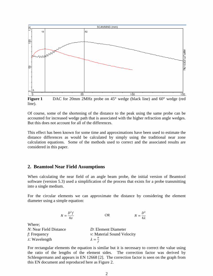
Abstract In a previous report by the authors, the relative accuracy of Beamtool as it relates to calculations of several beam parameters was considered. Comparison of the values obtained by Beamtool, to those obtained from Civa, indicated that the traditional approximations used in Beamtool were reasonably close to what might be predicted for actual probes. Deviation from the ideal was noted to occur for the near field length of some probe configurations that would be greater than desirable for even just a simple approximation. Real life experience as well as analytical modelling has indicated that the near zone of refracted transverse wave beams experiences a shortening as the refracted angle increases. This paper considers some of the various compensation techniques used to reduce the estimated near zone. Comparison of the various techniques is done using a variety of common probe frequencies and apertures. Keywords: Modelling, near field, validation, ultrasound, Civa 1. Introduction The authors have previously reported on the relative accuracy of the quantitative aspects of Beamtool [1] as it relates to calculations for refracted angle, beam divergence and near field length for both round and rectangular shaped elements. It was demonstrated that, in general, the values obtained by Beamtool compared well with those obtained from Civa. This indicated that the traditional approximations used in Beamtool were reasonably close to what might be predicted for actual probes. When the near field lengths were compared for a small sample of apertures and shapes that might be used in most applications, it was found that some were very close to the expected real values. However, for the larger values of near field some of the values estimated by Beamtool had deviations that might be considered more than tolerable as a simple first approximation for the purposes of technique development. Anyone who has been required to construct a distance amplitude correction (DAC) curve using a standard probe on interchangeable refracting wedges has noted that, for larger diameter probes, the peak of the curve tends to migrate to slightly shorter soundpaths when the same probe is used on higher angle refracting wedges. This effect is conformed using analytical modelling by Civa simulation software. Figure 1 indicates the DAC that would result for a 2MHz 20mm diameter element on a 45° and 60° refracting wedge. The black line indicates the DAC for the 45° and is seen to peak at 52mm. The DAC for the 60° wedge is represented by the red line and it peaks at 13mm.

www.ndt.net/?id=15673Vol.19 No.05 (May 2014) - The e-Journal of Nondestructive Testing - ISSN 1435-4934

www.ndt.net/?id=15673Vol.19 No.05 (May 2014) - The e-Journal of Nondestructive Testing - ISSN 1435-4934

www.ndt.net/?id=15673Vol.19 No.05 (May 2014) - The e-Journal of Nondestructive Testing - ISSN 1435-4934

www.ndt.net/?id=15766Vol.19 No.06 (June 2014) - The e-Journal of Nondestructive Testing - ISSN 1435-4934

2

Figure 1 DAC for 20mm 2MHz probe on 45° wedge (black line) and 60° wedge (red line). Of course, some of the shortening of the distance to the peak using the same probe can be accounted for increased wedge path that is associated with the higher refraction angle wedges. But this does not account for all of the differences. This effect has been known for some time and approximations have been used to estimate the distance differences as would be calculated by simply using the traditional near zone calculation equations. Some of the methods used to correct and the associated results are considered in this paper. 2. Beamtool Near Field Assumptions When calculating the near field of an angle beam probe, the initial version of Beamtool software (version 5.3) used a simplification of the process that exists for a probe transmitting into a single medium. For the circular elements we can approximate the distance by considering the element diameter using a simple equation:

� = ���4� OR � = ��

4�

Where; N: Near Field Distance D: Element Diameter f: Frequency v: Material Sound Velocity �: Wavelength � =

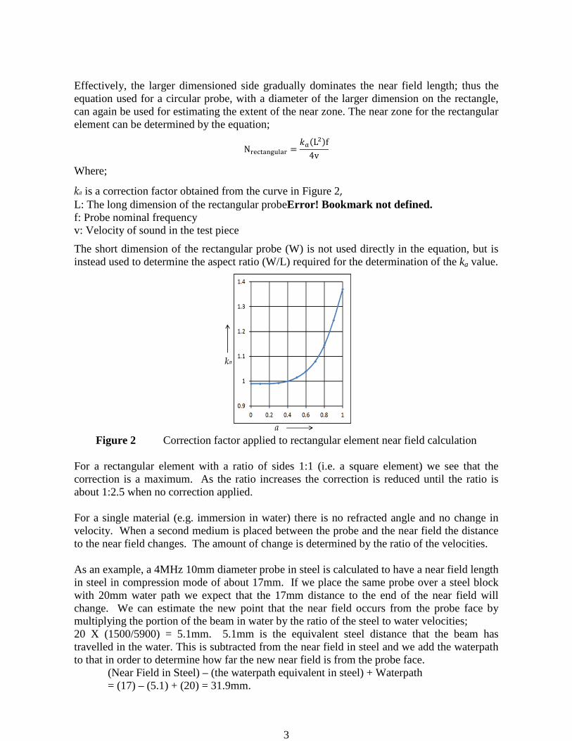
For rectangular elements the equation is similar but it is necessary to correct the value using the ratio of the lengths of the element sides. The correction factor was derived by Schlengermann and appears in EN 12668 [2]. The correction factor is seen on the graph from this EN document and reproduced here as Figure 2.

3

Effectively, the larger dimensioned side gradually dominates the near field length; thus the equation used for a circular probe, with a diameter of the larger dimension on the rectangle, can again be used for estimating the extent of the near zone. The near zone for the rectangular element can be determined by the equation;

N� ��������� = ���L��f4v

Where;

ka is a correction factor obtained from the curve in Figure 2, L: The long dimension of the rectangular probeError! Bookmark not defined. f: Probe nominal frequency v: Velocity of sound in the test piece

The short dimension of the rectangular probe (W) is not used directly in the equation, but is instead used to determine the aspect ratio (W/L) required for the determination of the ka value.

Figure 2 Correction factor applied to rectangular element near field calculation

For a rectangular element with a ratio of sides 1:1 (i.e. a square element) we see that the correction is a maximum. As the ratio increases the correction is reduced until the ratio is about 1:2.5 when no correction applied. For a single material (e.g. immersion in water) there is no refracted angle and no change in velocity. When a second medium is placed between the probe and the near field the distance to the near field changes. The amount of change is determined by the ratio of the velocities. As an example, a 4MHz 10mm diameter probe in steel is calculated to have a near field length in steel in compression mode of about 17mm. If we place the same probe over a steel block with 20mm water path we expect that the 17mm distance to the end of the near field will change. We can estimate the new point that the near field occurs from the probe face by multiplying the portion of the beam in water by the ratio of the steel to water velocities; 20 X (1500/5900) = 5.1mm. 5.1mm is the equivalent steel distance that the beam has travelled in the water. This is subtracted from the near field in steel and we add the waterpath to that in order to determine how far the new near field is from the probe face. (Near Field in Steel) – (the waterpath equivalent in steel) + Waterpath

= (17) – (5.1) + (20) = 31.9mm.

4

This is illustrated in Figure 3 where a probe is placed on a steel block and then placed 20mm above in water.

Figure 3 Change of near field distance with added waterpath

An assumption made in the initial version of Beamtool 5.3 was that this situation applies equally to wedge paths. By this is meant that when the probe is placed on a wedge the equivalent distance in the tested material is calculated for the wedge path and this distance is removed from the near field in the test material and the wedge path distance added to the geometric remainder. For example, a wedge that produces a refracted angle of 60° compression mode for the 10mm diameter 4MHz probe we used in Figure 3 might have a wedge path of 10.75mm. If the wedge material velocity is 2345 m/s the ratio of 2345/5900 is about 0.4. Multiply the wedge path by 0.4 and we get 4.3mm as the equivalent steel distance travelled in the wedge. As above for 0° incidence in water, we calculate for wedge plastic:

(Near Field in Steel) – (the wedge path equivalent in steel) + Wedge path = (17) – (4.3) + (10.75) = 23.45 mm.

This is the sort of value seen calculated with a wedge in Figure 4.

Figure 4 Change of near field distance with added wedge path

5

Values for the near zone calculated by the basic equations provided in level 1 ultrasonic training would use these basic equations and derive what we have considered to be “close approximations” to the actual values measured using the responses from point reflectors such as a steel ball in immersion assessments or side drilled holes in contact testing. When a more accurate assessment is made using the interference patterns in an analytical calculation, we can see that the “rule of thumb” equations are not always predicting the same value. Even for the simple immersion condition we can see deviation from the simple equation. Consider our example of a 10mm diameter 4MHz probe pulsed into water. The standard

equation � = ��� predicts a near field distance of 67mm. The Civa model using water at

1483m/s will provide a near field in water of about 67mm for a probe with a 50% bandwidth. This is seen in Figure 5 and compares well with the value derived from the simple equation.

Figure 5 67mm near field distance for 4MHz 10mm diameter in water at 50% BW

When the probe is placed over a steel block and we assess the location of the near field with a normal incidence from water, the location plots as 33mm from the probe. This is within 1mm of that predicted by Beamtool in Figure 3. The Civa plot is seen as Figure 6.

Figure 6 33mm near field distance for 4MHz 10mm diameter in steel 20mm waterpath

6

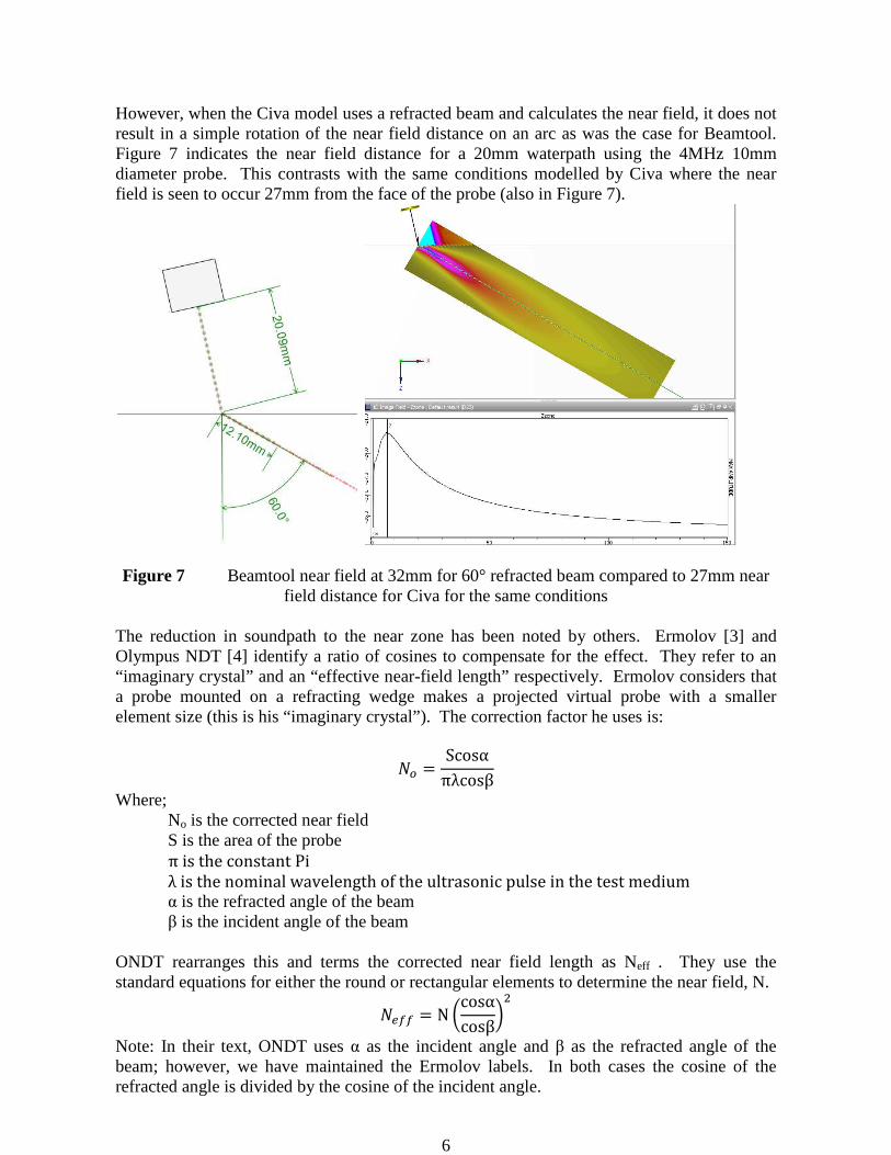
However, when the Civa model uses a refracted beam and calculates the near field, it does not result in a simple rotation of the near field distance on an arc as was the case for Beamtool. Figure 7 indicates the near field distance for a 20mm waterpath using the 4MHz 10mm diameter probe. This contrasts with the same conditions modelled by Civa where the near field is seen to occur 27mm from the face of the probe (also in Figure 7).

Figure 7 Beamtool near field at 32mm for 60° refracted beam compared to 27mm near

field distance for Civa for the same conditions The reduction in soundpath to the near zone has been noted by others. Ermolov [3] and Olympus NDT [4] identify a ratio of cosines to compensate for the effect. They refer to an “imaginary crystal” and an “effective near-field length” respectively. Ermolov considers that a probe mounted on a refracting wedge makes a projected virtual probe with a smaller element size (this is his “imaginary crystal”). The correction factor he uses is:

�� = Scosαπλcosβ

Where; No is the corrected near field S is the area of the probe π is the constant Pi λ is the nominal wavelength of the ultrasonic pulse in the test medium α is the refracted angle of the beam β is the incident angle of the beam

ONDT rearranges this and terms the corrected near field length as Neff . They use the standard equations for either the round or rectangular elements to determine the near field, N.

�8 = N 9cosαcosβ:

�

Note: In their text, ONDT uses α as the incident angle and β as the refracted angle of the beam; however, we have maintained the Ermolov labels. In both cases the cosine of the refracted angle is divided by the cosine of the incident angle.

7

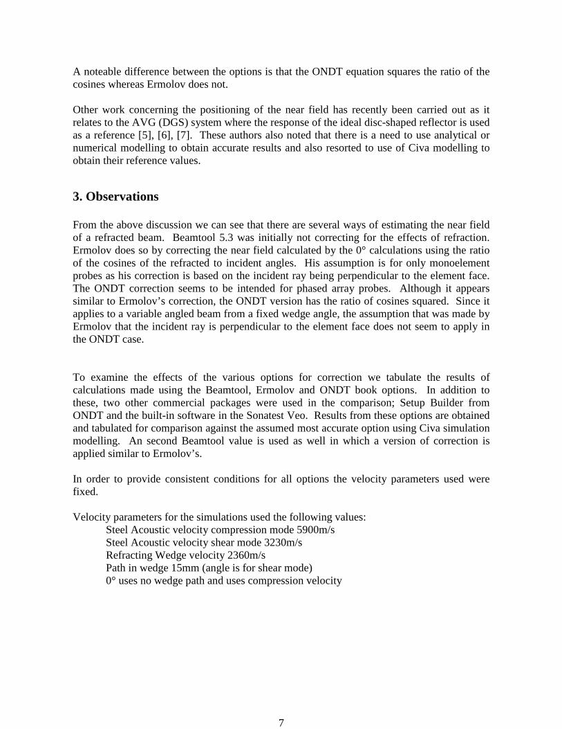
A noteable difference between the options is that the ONDT equation squares the ratio of the cosines whereas Ermolov does not. Other work concerning the positioning of the near field has recently been carried out as it relates to the AVG (DGS) system where the response of the ideal disc-shaped reflector is used as a reference [5], [6], [7]. These authors also noted that there is a need to use analytical or numerical modelling to obtain accurate results and also resorted to use of Civa modelling to obtain their reference values.

3. Observations From the above discussion we can see that there are several ways of estimating the near field of a refracted beam. Beamtool 5.3 was initially not correcting for the effects of refraction. Ermolov does so by correcting the near field calculated by the 0° calculations using the ratio of the cosines of the refracted to incident angles. His assumption is for only monoelement probes as his correction is based on the incident ray being perpendicular to the element face. The ONDT correction seems to be intended for phased array probes. Although it appears similar to Ermolov’s correction, the ONDT version has the ratio of cosines squared. Since it applies to a variable angled beam from a fixed wedge angle, the assumption that was made by Ermolov that the incident ray is perpendicular to the element face does not seem to apply in the ONDT case. To examine the effects of the various options for correction we tabulate the results of calculations made using the Beamtool, Ermolov and ONDT book options. In addition to these, two other commercial packages were used in the comparison; Setup Builder from ONDT and the built-in software in the Sonatest Veo. Results from these options are obtained and tabulated for comparison against the assumed most accurate option using Civa simulation modelling. An second Beamtool value is used as well in which a version of correction is applied similar to Ermolov’s. In order to provide consistent conditions for all options the velocity parameters used were fixed. Velocity parameters for the simulations used the following values: Steel Acoustic velocity compression mode 5900m/s Steel Acoustic velocity shear mode 3230m/s Refracting Wedge velocity 2360m/s Path in wedge 15mm (angle is for shear mode) 0° uses no wedge path and uses compression velocity

8

Near fields distance is tabulated in mm from the wedge –steel interface Table 1 Probe Parameters Near Field Length Method

Freq

(MHz)

Angle

(°)

Diameter

/Rectangle (H x

W) mm

ESBT

5.3

ESBT-

corrected

Ermolov* ONDT

Book

Veo Builder Civa

2 0°

(Comp)

6 3.1 3.1 3.1 3.1 1.25 2.7 2

45°

shear

6 NA NA NA NA NA NA NA

60°

shear

6 NA NA NA NA NA NA NA

70°

shear

6 NA NA NA NA NA NA NA

NA denotes that with a 15mm wedge path the near zone occurs inside the wedge *Ermolov’s equation for the near field is based solely on the area of a probe and he limits the assumption to a 2:1 length by width ratio. Table 2 Probe Parameters Near Field Length Method

Freq

(MHz)

Angle

(°)

Diameter

/Rectangle

(H x W)

mm

ESBT-

5.3

ESBT-

corrected

Ermolov ONDT

Book

Veo Builder Civa

2 0°

Comp.

10 8.5 8.5 8.5 8.5 6.8 7.72 8.5

45°

shear

10 5 4 6 10 NA 1 5

60°

shear

10 5 3 2 6 NA NA 3

70°

shear

10 5 2 NA 1 NA NA 3

NA denotes that with a 15mm wedge path the near zone occurs inside the wedge Table 3 Probe Parameters Near Field Length Method

Freq

(MHz)

Angle

(°)

Diameter

/Rectangle

(H x W)

mm

ESBT-

5.3

ESBT-

corrected

Ermolov ONDT

Book

Veo Builder Civa

2 0°

Comp.

20 34 34 34 34 36 31 34

45°

shear

20 51 42 40 49 36 29 47

60°

shear

20 51 33 28 40 23 16 40

70°

shear

20 51 24 16 28 2 7 31

9

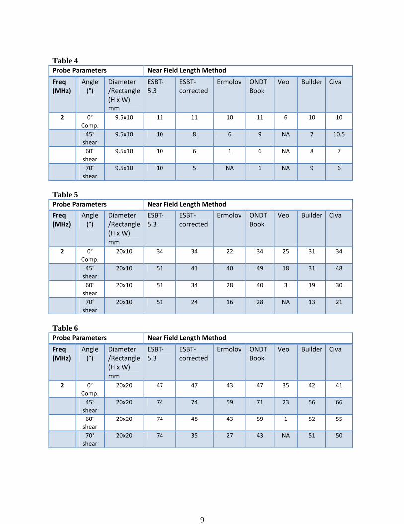
Table 4 Probe Parameters Near Field Length Method

Freq

(MHz)

Angle

(°)

Diameter

/Rectangle

(H x W)

mm

ESBT-

5.3

ESBT-

corrected

Ermolov ONDT

Book

Veo Builder Civa

2 0°

Comp.

9.5x10 11 11 10 11 6 10 10

45°

shear

9.5x10 10 8 6 9 NA 7 10.5

60°

shear

9.5x10 10 6 1 6 NA 8 7

70°

shear

9.5x10 10 5 NA 1 NA 9 6

Table 5 Probe Parameters Near Field Length Method

Freq

(MHz)

Angle

(°)

Diameter

/Rectangle

(H x W)

mm

ESBT-

5.3

ESBT-

corrected

Ermolov ONDT

Book

Veo Builder Civa

2 0°

Comp.

20x10 34 34 22 34 25 31 34

45°

shear

20x10 51 41 40 49 18 31 48

60°

shear

20x10 51 34 28 40 3 19 30

70°

shear

20x10 51 24 16 28 NA 13 21

Table 6 Probe Parameters Near Field Length Method

Freq

(MHz)

Angle

(°)

Diameter

/Rectangle

(H x W)

mm

ESBT-

5.3

ESBT-

corrected

Ermolov ONDT

Book

Veo Builder Civa

2 0°

Comp.

20x20 47 47 43 47 35 42 41

45°

shear

20x20 74 74 59 71 23 56 66

60°

shear

20x20 74 48 43 59 1 52 55

70°

shear

20x20 74 35 27 43 NA 51 50

10

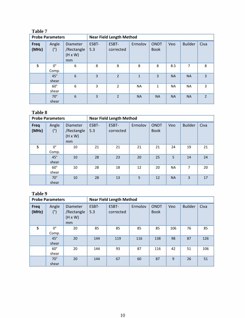
Table 7 Probe Parameters Near Field Length Method

Freq

(MHz)

Angle

(°)

Diameter

/Rectangle

(H x W)

mm

ESBT-

5.3

ESBT-

corrected

Ermolov ONDT

Book

Veo Builder Civa

5 0°

Comp.

6 8 8 8 8 8.5 7 8

45°

shear

6 3 2 1 3 NA NA 3

60°

shear

6 3 2 NA 1 NA NA 3

70°

shear

6 3 2 NA NA NA NA 2

Table 8 Probe Parameters Near Field Length Method

Freq

(MHz)

Angle

(°)

Diameter

/Rectangle

(H x W)

mm

ESBT-

5.3

ESBT-

corrected

Ermolov ONDT

Book

Veo Builder Civa

5 0°

Comp.

10 21 21 21 21 24 19 21

45°

shear

10 28 23 20 25 5 14 24

60°

shear

10 28 18 12 20 NA 7 20

70°

shear

10 28 13 5 12 NA 3 17

Table 9 Probe Parameters Near Field Length Method

Freq

(MHz)

Angle

(°)

Diameter

/Rectangle

(H x W)

mm

ESBT-

5.3

ESBT-

corrected

Ermolov ONDT

Book

Veo Builder Civa

5 0°

Comp.

20 85 85 85 85 106 76 85

45°

shear

20 144 119 116 138 98 87 126

60°

shear

20 144 93 87 116 42 51 106

70°

shear

20 144 67 60 87 9 26 51

11

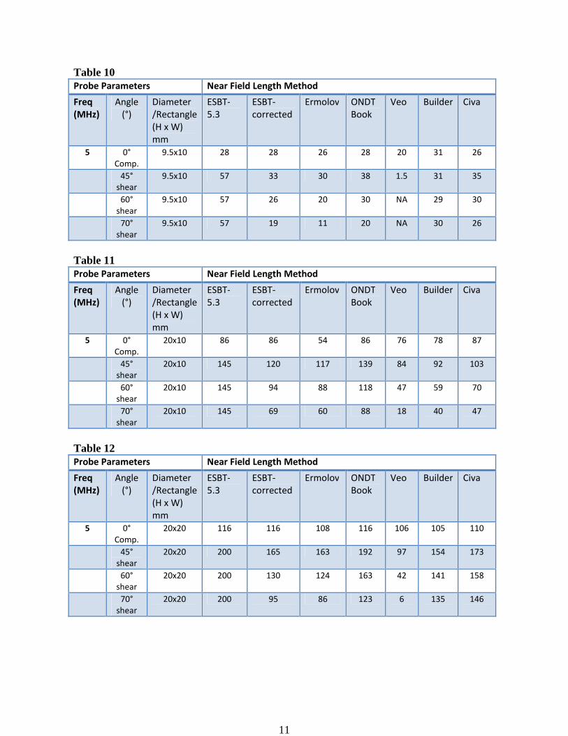
Table 10 Probe Parameters Near Field Length Method

Freq

(MHz)

Angle

(°)

Diameter

/Rectangle

(H x W)

mm

ESBT-

5.3

ESBT-

corrected

Ermolov ONDT

Book

Veo Builder Civa

5 0°

Comp.

9.5x10 28 28 26 28 20 31 26

45°

shear

9.5x10 57 33 30 38 1.5 31 35

60°

shear

9.5x10 57 26 20 30 NA 29 30

70°

shear

9.5x10 57 19 11 20 NA 30 26

Table 11 Probe Parameters Near Field Length Method

Freq

(MHz)

Angle

(°)

Diameter

/Rectangle

(H x W)

mm

ESBT-

5.3

ESBT-

corrected

Ermolov ONDT

Book

Veo Builder Civa

5 0°

Comp.

20x10 86 86 54 86 76 78 87

45°

shear

20x10 145 120 117 139 84 92 103

60°

shear

20x10 145 94 88 118 47 59 70

70°

shear

20x10 145 69 60 88 18 40 47

Table 12 Probe Parameters Near Field Length Method

Freq

(MHz)

Angle

(°)

Diameter

/Rectangle

(H x W)

mm

ESBT-

5.3

ESBT-

corrected

Ermolov ONDT

Book

Veo Builder Civa

5 0°

Comp.

20x20 116 116 108 116 106 105 110

45°

shear

20x20 200 165 163 192 97 154 173

60°

shear

20x20 200 130 124 163 42 141 158

70°

shear

20x20 200 95 86 123 6 135 146

12

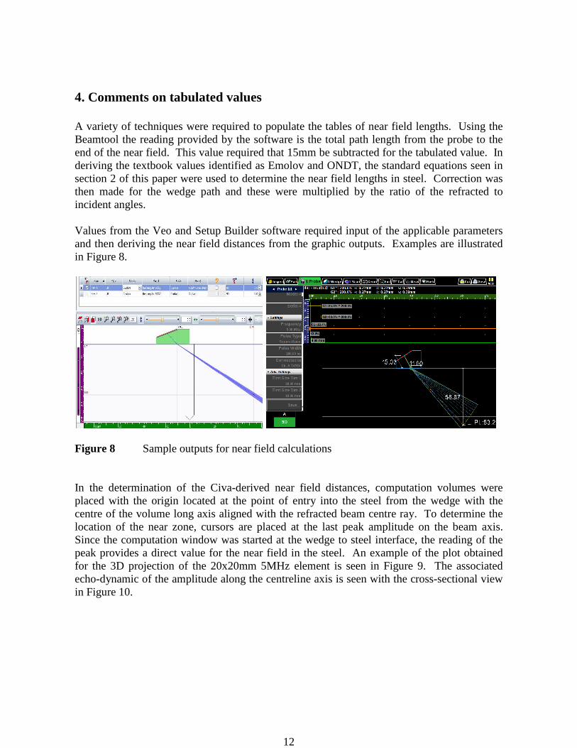
4. Comments on tabulated values A variety of techniques were required to populate the tables of near field lengths. Using the Beamtool the reading provided by the software is the total path length from the probe to the end of the near field. This value required that 15mm be subtracted for the tabulated value. In deriving the textbook values identified as Emolov and ONDT, the standard equations seen in section 2 of this paper were used to determine the near field lengths in steel. Correction was then made for the wedge path and these were multiplied by the ratio of the refracted to incident angles. Values from the Veo and Setup Builder software required input of the applicable parameters and then deriving the near field distances from the graphic outputs. Examples are illustrated in Figure 8.

Figure 8 Sample outputs for near field calculations In the determination of the Civa-derived near field distances, computation volumes were placed with the origin located at the point of entry into the steel from the wedge with the centre of the volume long axis aligned with the refracted beam centre ray. To determine the location of the near zone, cursors are placed at the last peak amplitude on the beam axis. Since the computation window was started at the wedge to steel interface, the reading of the peak provides a direct value for the near field in the steel. An example of the plot obtained for the 3D projection of the 20x20mm 5MHz element is seen in Figure 9. The associated echo-dynamic of the amplitude along the centreline axis is seen with the cross-sectional view in Figure 10.

13

Figure 9 3D plot of pressure boundaries of 20x20mm 5MHz probe with 15mm wedge-path on steel

Figure 10 2D view of pressure boundaries of 20x20mm 5MHz probe with 15mm wedge-path on steel (above) with centre-axis plot of amplitude (below) peaked at 168mm Of particular interest to phased-array users is how close these estimates might be when using linear array probes. It is assumed that the critical factor is merely the aperture. However, there is a slight difference between monoelmeent rectangular probes and the same size aperture linear array probes. Whereas the monoelement probe is mounted on a fixed angle

14

wedge and that angle used in the corrections using the ratio of cosines, the incident angle of the beam formed in a linear array phased-array probe is not the same as the wedge incident angle in a monoelement probe except for the condition where there are no delays applied to the elements. As a check on the differences, a phased-array example was run to determine the resultant near field distance when using the same 15mm wedge path with a 5MHz linear array probe. The probe modelled was a 64 element 5MHz probe with a 0.6mm pitch. It was mounted on a cross-linked polystyrene wedge with an incident angle that produces a natural refracted angle of 55°. In Figure 11 and the associated table of values below it we see that the Civa simulated near field for the phased-array probe is nearly the same as for the monoelement probe of the same aperture in spite of the slight wedge angle difference.

Figure 11 9.5x10mm aperture Phased-array 64 element 5MHz Table 13 Probe Parameters Near Field Length Method

Freq

(MHz)

Angle

(°)

Diameter

/Rectangle

(H x W)

mm

ESBT-

5.3

ESBT-

corrected

Ermolov ONDT

Book

Veo Builder Civa

Phased-

array

model

5 45°

shear

9.5x10 54 33 30 38 1.5 31 36

60°

shear

9.5x10 54 26 20 30 NA 29 31

70°

shear

9.5x10 54 19 11 20 NA 30 28

15

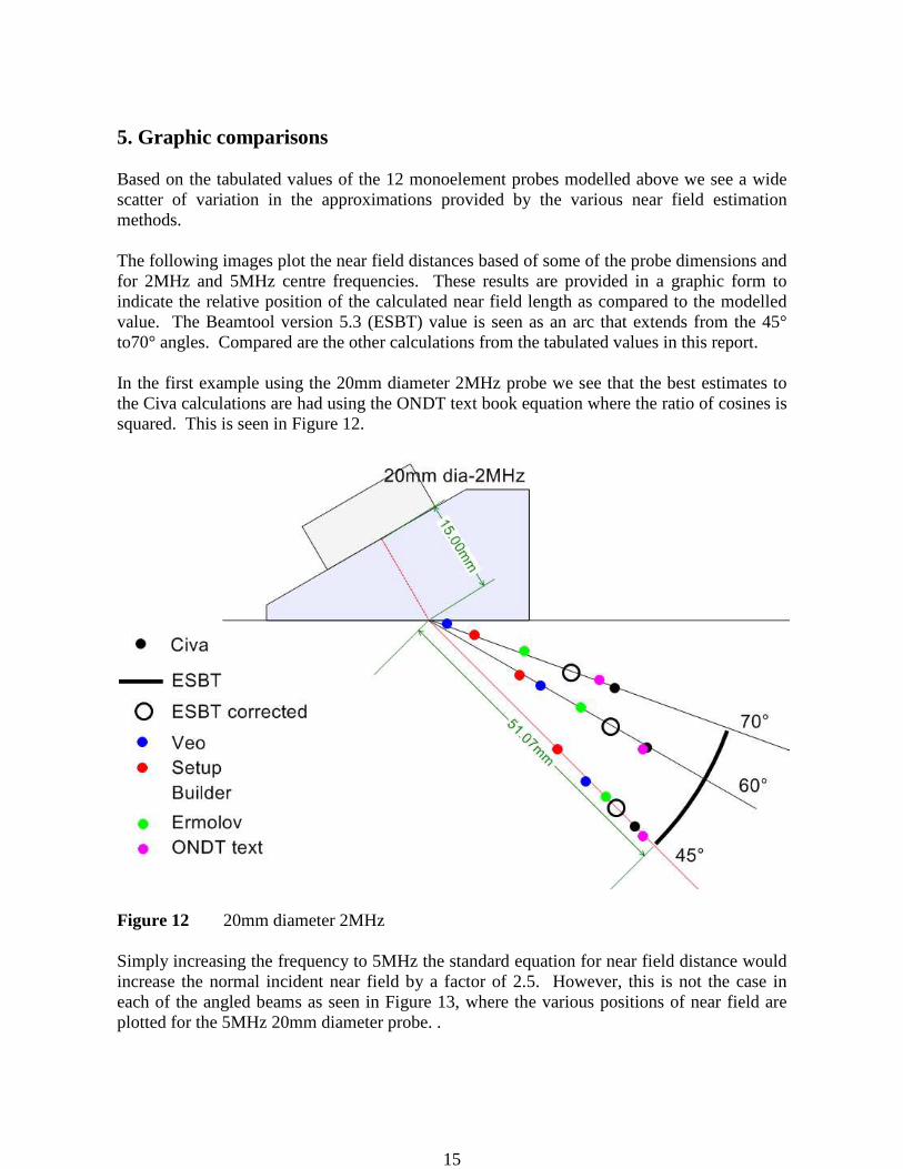
5. Graphic comparisons Based on the tabulated values of the 12 monoelement probes modelled above we see a wide scatter of variation in the approximations provided by the various near field estimation methods. The following images plot the near field distances based of some of the probe dimensions and for 2MHz and 5MHz centre frequencies. These results are provided in a graphic form to indicate the relative position of the calculated near field length as compared to the modelled value. The Beamtool version 5.3 (ESBT) value is seen as an arc that extends from the 45° to70° angles. Compared are the other calculations from the tabulated values in this report. In the first example using the 20mm diameter 2MHz probe we see that the best estimates to the Civa calculations are had using the ONDT text book equation where the ratio of cosines is squared. This is seen in Figure 12.

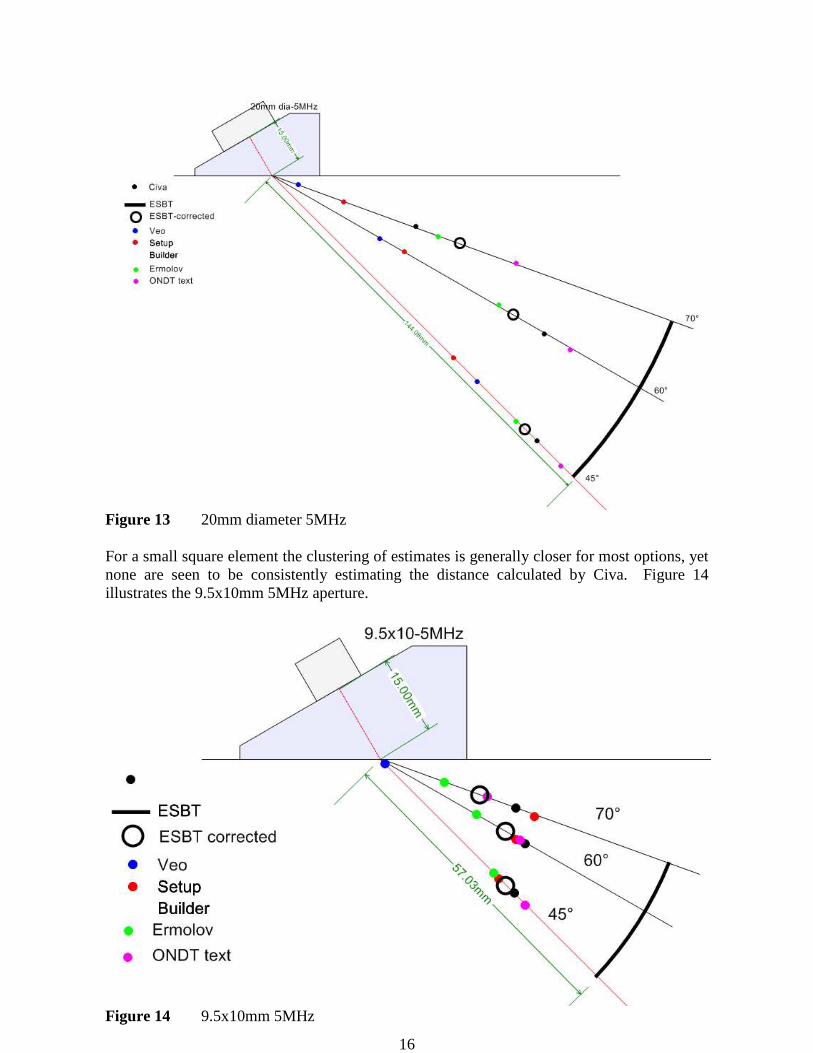
Figure 12 20mm diameter 2MHz Simply increasing the frequency to 5MHz the standard equation for near field distance would increase the normal incident near field by a factor of 2.5. However, this is not the case in each of the angled beams as seen in Figure 13, where the various positions of near field are plotted for the 5MHz 20mm diameter probe. .

16

Figure 13 20mm diameter 5MHz For a small square element the clustering of estimates is generally closer for most options, yet none are seen to be consistently estimating the distance calculated by Civa. Figure 14 illustrates the 9.5x10mm 5MHz aperture.

Figure 14 9.5x10mm 5MHz

17

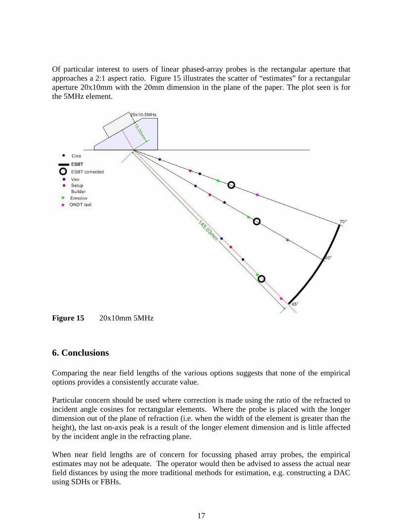
Of particular interest to users of linear phased-array probes is the rectangular aperture that approaches a 2:1 aspect ratio. Figure 15 illustrates the scatter of “estimates” for a rectangular aperture 20x10mm with the 20mm dimension in the plane of the paper. The plot seen is for the 5MHz element.

Figure 15 20x10mm 5MHz

6. Conclusions Comparing the near field lengths of the various options suggests that none of the empirical options provides a consistently accurate value. Particular concern should be used where correction is made using the ratio of the refracted to incident angle cosines for rectangular elements. Where the probe is placed with the longer dimension out of the plane of refraction (i.e. when the width of the element is greater than the height), the last on-axis peak is a result of the longer element dimension and is little affected by the incident angle in the refracting plane. When near field lengths are of concern for focussing phased array probes, the empirical estimates may not be adequate. The operator would then be advised to assess the actual near field distances by using the more traditional methods for estimation, e.g. constructing a DAC using SDHs or FBHs.

18

7. Acknowledgements We would like to thank Ali Golshani Ekhlas of Pars Leading Inspection Company, Ekbatan, Tehran, Iran for bringing this issue to our attention. Ali also provided some of the values for the manufacturer’s software outputs used for comparisons. References

1. E. Ginzel, M. Matheson, P. Cyr, B. Brown, Validation of aspects of Beamtool, NDT.net, 2014

2. EN 12668 - Non-destructive testing - Characterization and verification of ultrasonic examination equipment - Part 2: Probes

3. I. N. Ermolov, A. Vopilkin, V. Badlyan, Calculations in Ultrasonic Testing – Brief Handbook, Scientific and Production Center ECHO+, Moscow, 2000

4. Olympus NDT, Introduction to phased array ultrasonic technology applications – R/D Tech guideline, ONDT, Canada, 2007

5. X. Yan, J. Zhang, D. Kass, P. Lamglois, DGS Sizing Diagram with Single Element and Phased Array Angle Beam Probe, http://www.ndt.net/article/ndtnet/2010/14_Yan.pdf, NDT.net, Nov. 2010

6. W. Kleinert, Y. Oberdoefer, G. Splitt, The Ideal Angle Beam Probe for DGS Evaluation, http://www.ndt.net/article/ecndt2010/reports/1_03_64.pdf, NDT.net, August, 2010

7. Y. Oberdoefer, G. Splitt,W. Kleinert, Novel Single-Element and Phased Array Angle Beam Probes for Enhanced DGS Sizing, http://www.ndt.net/article/jrc-nde2010/papers/75.pdf, NDT.net, April 2012