Near-Feasible Stable Matchings with Couples

Thanh Nguyen∗ and Rakesh Vohra†

August 2015, this version January 2017

Abstract

The National Resident Matching program seeks a stable matching of medical stu-

dents to teaching hospitals. With couples, stable matchings need not exist. Neverthe-

less, for any student preferences, we show that each instance of a matching problem

has a ‘nearby’ instance with a stable matching. The nearby instance is obtained by

perturbing the capacities of the hospitals. Given a reported capacity kh for each hos-

pital h, we find a redistribution of the slot capacities, k∗h, satisfying |kh−k∗h| ≤ 2 for all

hospitals h and∑

h kh ≤∑

k∗h ≤∑

h kh + 4, such that a stable matching exists with

respect to k∗.

Keywords: stable matching, complementarities, Scarf’s lemma

JEL classification: C78, D47

1 Introduction

Each year, about 20,000 medical school graduates are matched to teaching hospitals via the

National Resident Match Program (NRMP).1 This service has been in operation since 1952

and its longevity is ascribed to the fact that the matching produced is stable (Roth [1984]).

Stability means no doctor-hospital pair can improve their outcomes by matching with each

other outside the NRMP.2

∗Krannert School of Management, Purdue University, nguye161@purdue.edu†University of Pennsylvania, rvohra@seas.upenn.edu1http://www.nrmp.org/wp-content/uploads/2014/04/Main-Match-Results-and-Data-2014.pdf2Stability is now an important desiderata in the design of matching markets. See Fleiner [2003], Hatfield

and Milgrom [2005], Ostrovsky [2008] and Hatfield and Kojima [2010].

1

With the presence of couples who submit joint preference lists over pairs of hospitals,

a stable matching need not exist (see Roth [1984]). Even determining whether a stable

matching exists is NP-hard. Roth and Peranson [1999] proposed a heuristic modification

of the algorithm then in place to accommodate couples’ preferences. It has, without fail,

returned matches that are stable with respect to reported preferences. However, Ashlagi

et al. [2014] and Biro et al. [2013] have shown, in separate settings that as the proportion of

couples increases, this algorithm frequently fails to terminate in a stable matching. In the

NRMP, the proportion of couples is between 5% and 10%, but elsewhere, the proportion of

couples is as high as 40% (see Biro and Klijn [2013]). Resident matching is not the only

setting with a “couples” problem. Biro et al. [2013] points to the task of assigning high

school teachers in Hungary to majors, where almost all teachers need to be assigned to two

majors.

In this paper we propose to deal with this difficulty by treating the hospital capacity

constraints as ‘soft’. We show for any instance of the stable matching problem with couples,

there is a ‘nearby’ instance guaranteed to have a stable matching. Furthermore, we give

an algorithm for determining it. This nearby instance is obtained by altering the initial

capacities of the hospitals.

Adjusting the capacities of hospitals is not uncommon. The NRMP allows hospitals to

choose if they wish to be matched with an even or odd number of students. Thus, capacity

constraints can be modified by at least 1. In fact, slots are sometimes reallocated between

hospitals.3 Further, in some specialities where supply outstrips demand, slots go unfilled.

In these cases, hospitals have ‘work arounds’, one of which is to use the money that would

have gone to the unfilled slot to incentivize existing doctors to ‘pick up the slack’.

To formalize the notion of nearby, call a matching α-feasible if the number of slots

allocated by each hospital to doctors differs (up or down) from its actual capacity by at

most α. Our iterative rounding (IR) algorithm returns a 2-feasible stable matching that

3https://www.acponline.org/advocacy/where_we_stand/assets/iii4-redistribution-

graduate-medica-education-slots.pdf

2

neither decreases the total number of slots nor increases it by more than 4 (Theorem 2.1).

This guarantee does not depend on any restriction in the preferences of doctors (single or

otherwise) and is independent of the size of the instance.

Regarding a possible increase of at most 4 slots in total, every additional resident, ac-

cording to the American Medical Association, costs about $100,000 on average. The bulk of

the funding for such positions comes from the US Government via Medicaid. Currently, the

total expenditure on resident training is upward of $10 billions.4

A reduction of up to 2 slots in a small hospital’s capacity could be dramatic. In internal

medicine, for example, the number of slots can be as small as 4 and as large as 30.5 However,

programs with a small number of slots tend to be concentrated in rural areas. Couples

participating in the NRMP are advised to apply to urban areas with many hospitals so as

to increase their chances of obtaining positions close to each other. Our algorithm has the

property that if no couple applies to a rural hospital, then that rural hospital’s capacities

are unchanged (Theorem 2.2).

Preliminary simulations of our algorithm suggest that only a very small fraction of hospi-

tals see a change in their capacities.6 The first set of experiments was based on 200 randomly

generated instances involving 270 doctors and 18 hospitals and four different proportions of

couples. The total capacity of hospitals ranged between 75% and 90% of the number of

applicants, consistent with ratios observed over the last decade. Hospitals had the same

randomly generated priority ordering over individual doctors. Hospitals were arbitrarily

assigned to one of 5 regions. Preferences on the doctor side admit a degree of positive cor-

relation. Couples preferences were generated in a way that 70% of them prefer to be in the

same region.

4These numbers are from an AMA pamphlet in support of the current approach to funding res-idency programs. http://savegme.org/wp-content/uploads/2013/01/graduate-medical-education-

action-kit.2-3.pdf5See http://www.nrmp.org/wp-content/uploads/2015/05/Main-Match-Results-and-Data-

2015_final.pdf.6A comprehensive test of the IR is beyond the scope of this paper. The results we report are based on

work in progress joint with Dengwang Tang and Vijay Subramaniam.

3

When the proportion of couples is 10% (roughly the current proportion in the NRMP),

97% of all hospitals (out of all 18×200 trials) saw no change in their capacity. Over the same

instances, fewer than 1 % of hospitals saw an increase in capacity of upto 2. Fewer than 1%

saw a decrease in capacity. When the proportion of couples was 90 %, 80% of hospitals saw

no change in capacities. No more than 9% of the hospitals saw an increase in capacity. At

most 9% saw a decrease in capacity of 1 and less than 0.3% saw a decrease of 2.

The second set of experiments are on 1000 instances involving 500 doctors, kindly pro-

vided by Peter Biro. These instances are known to have stable matchings because couples

are endowed with weakly responsive preferences(see Klaus and Klijn [2005]). This was done

to determine how well the IR algorithm performs on instances where a stable match is known

to exists.7 On these instances, the IR algorithm always returns an exact stable matching.

Biro et al. [2013] report that the Roth and Peranson algorithm frequently fails to terminate

in a stable matching on these instances when a high proportion of couples are present. In

their experiments, with at least 175 couples, the Roth and Peranson algorithm failed to find

a stable matching in at least 90% of the 1000 instances.8

Unlike all prior algorithms employed in matching problems (with the exception of Biro

et al. [2013]), our algorithm does not use the deferred acceptance (DA) algorithm introduced

in Gale and Shapley [1962]. It employs, instead, a combination of Scarf’s lemma (Scarf

[1967]) and the iterative rounding method, developed in Lau et al. [2011] and Nguyen et al.

[2016]. In the first stage, Scarf’s lemma is used to extend the notion of stability to fractional

matchings as well as to identify a fractional matching that is stable.9 In the second stage,

this fractional matching is carefully rounded into an actual matching such that stability is

preserved.10

7The Roth and Peranson algorithm is also not guaranteed to find a stable matching if one exists.8The need to deal with a large proportion of couples arises in other matching settings like assigning

teachers to pairs of courses in Hungary (see Biro et al. [2013]).9Biro et al. [2013] also use Scarf’s lemma and in their simulations report how often the matching returned

is integral.10Our approach, while constructive, relies on Scarf’s lemma, which is PPAD complete, Kintali [2008].

Thus, it has a worst-case complexity equivalent to that of computing a fixed point. This is not a barrierto implementation. For example, building on Budish [2011], a course allocation scheme that relies on a

4

Below, we discuss the related literature. In Section 2, we give a formal definition of the

stable matching problem with couples. Section 3 states Scarf’s lemma and formulates the

matching problem in a way to invoke the lemma. Section 4 outlines the IR in this context.

Section 5 concludes. Proofs are given in the Appendix.

Related work.

Roth [1984] establishes the non-existence of a stable matching when some agents are

couples. Subsequently, the more general problem of matching in the presence of complemen-

tarities has become an important topic. See Biro and Klijn [2013] for a brief survey. The

literature has taken four approaches to circumventing the problem of non-existence.

• Restrict couple’s preferences to ensure the existence of a stable matching (Cantala

[2004], Klaus and Klijn [2005], Pycia [2012], and Sethuraman et al. [2006].)

These restrictions rule out very many plausible preferences.

• Argue that instances of non-existence are rare in large markets.

Kojima et al. [2013] and Ashlagi et al. [2014] show that in a setting where applicant

preferences are drawn independently from a distribution, as the size of the market

increases and the proportion of couples approaches 0, the Roth and Peranson algorithm

terminates in a stable matching. But, Ashlagi et al. [2014] shows that when the

proportion of couples is positive, the probability that no stable matching exists is

bounded away from 0 even when the market’s size increases.

• Ignore the indivisibility of agents and provide interpretations of “fractional” stable

matchings (Dean et al. [2006], Aharoni and Holzman [1998], Aharoni and Fleiner [2003],

Kiraly and Pap [2008], and Biro and Fleiner [2016]).

Dean et al. [2006] is closest to this paper. It solves a restricted instance of the stable

matching problem with couples. In that instance, couples prefer to be together, rather

than apart, and a hospital must accept either both members of the couple or none.

fixed-point computation has been proposed and implemented at the Wharton School.

5

This restriction considerably simplifies the problem because each blocking constraint

only involves the preferences of a single hospital.11 Dean et al. [2006] adapt the DA

algorithm to identify a stable matching that is 2-feasible. They are unable to bound

the aggregate increase in capacity.12

• Modify the notion of stability (Klijn and Masso [2003], Jiang and Tan [2014], Manlove

et al. [2016].)

The modifications need not capture the original spirit of the notion of stability.

2 Matching with Couples and Main Result

In this section we describe the standard matching model with couples, that is studied, for

example, in Roth [1984] and Kojima et al. [2013]. Let H be the set of hospitals, D1 be the

set of single doctors, and D2 the set of couples. Let D be the set of all doctors listed as

individuals. Each single doctor in D has a strict preference ordering over H and her outside

option. Each couple in D has a strict preference ordering over ordered pairs of hospitals as

well as their outside option, denoted as ∅. The need for ordered pairs arises because couples

will have preferences over which member is assigned to which hospital.

Each hospital h ∈ H has a fixed capacity kh > 0. The preference of a hospital h over

subsets of doctors is assumed to be responsive. This means that h has a strict priority

ordering �h over elements of D and its outside option, which is denoted as ∅. A doctor

ranked above the outside option by the priority ordering is said to be feasible. For any set

D∗ ⊂ D, hospital h selects upto the kh highest priority feasible doctors in D∗.

A matching µ is an assignment of each single doctor to a hospital or his/her outside

option, an assignment of couples to at most two positions (in the same or different hospitals)

or their outside option, such that the total number of doctors assigned to any hospital h does

11In fact, many sources advise couples not to apply to the same specialty at a hospital to avoid beingscheduled in such a way that they do not see each other.

12The techniques in this paper can be used to generate a 1-feasible matching with a bound on the increasein aggregate capacity for this setting.

6

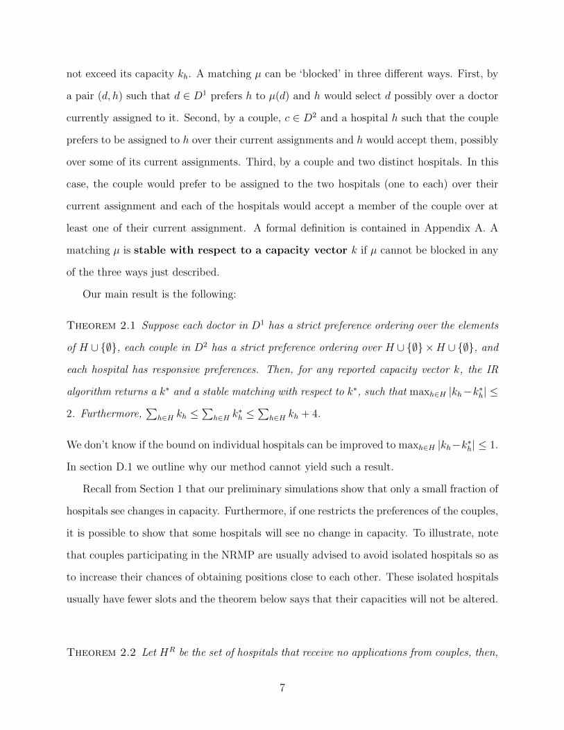
not exceed its capacity kh. A matching µ can be ‘blocked’ in three different ways. First, by

a pair (d, h) such that d ∈ D1 prefers h to µ(d) and h would select d possibly over a doctor

currently assigned to it. Second, by a couple, c ∈ D2 and a hospital h such that the couple

prefers to be assigned to h over their current assignments and h would accept them, possibly

over some of its current assignments. Third, by a couple and two distinct hospitals. In this

case, the couple would prefer to be assigned to the two hospitals (one to each) over their

current assignment and each of the hospitals would accept a member of the couple over at

least one of their current assignment. A formal definition is contained in Appendix A. A

matching µ is stable with respect to a capacity vector k if µ cannot be blocked in any

of the three ways just described.

Our main result is the following:

Theorem 2.1 Suppose each doctor in D1 has a strict preference ordering over the elements

of H ∪ {∅}, each couple in D2 has a strict preference ordering over H ∪ {∅} ×H ∪ {∅}, and

each hospital has responsive preferences. Then, for any reported capacity vector k, the IR

algorithm returns a k∗ and a stable matching with respect to k∗, such that maxh∈H |kh−k∗h| ≤

2. Furthermore,∑

h∈H kh ≤∑

h∈H k∗h ≤

∑h∈H kh + 4.

We don’t know if the bound on individual hospitals can be improved to maxh∈H |kh−k∗h| ≤ 1.

In section D.1 we outline why our method cannot yield such a result.

Recall from Section 1 that our preliminary simulations show that only a small fraction of

hospitals see changes in capacity. Furthermore, if one restricts the preferences of the couples,

it is possible to show that some hospitals will see no change in capacity. To illustrate, note

that couples participating in the NRMP are usually advised to avoid isolated hospitals so as

to increase their chances of obtaining positions close to each other. These isolated hospitals

usually have fewer slots and the theorem below says that their capacities will not be altered.

Theorem 2.2 Let HR be the set of hospitals that receive no applications from couples, then,

7

the IR algorithm can be modified so that in addition to the guarantees in Theorem 2.1, k∗h = kh

for all h ∈ HR.

The proof of Theorem 2.2 may be found in Appendix E.

In contrast to the Roth and Peranson algorithm, our algorithm is always guaranteed to

return a stable matching. However, unlike Roth and Peranson, it must perturb the capacities

of the hospitals. Simulations and analysis show that the the Roth and Peranson algorithm

frequently fails to terminate in a stable matching as the proportion of couples increases. The

performance guarantees of Theorem 2.1 and 2.2, however, do not depend on the proportion

of couples.

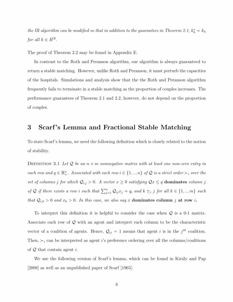
3 Scarf’s Lemma and Fractional Stable Matching

To state Scarf’s lemma, we need the following definition which is closely related to the notion

of stability.

Definition 3.1 Let Q be an n×m nonnegative matrix with at least one non-zero entry in

each row and q ∈ Rn+. Associated with each row i ∈ {1, .., n} of Q is a strict order �i over the

set of columns j for which Qi,j > 0. A vector x ≥ 0 satisfying Qx ≤ q dominates column j

of Q if there exists a row i such that∑n

j=1Qijxj = qi and k �i j for all k ∈ {1, ..,m} such

that Qi,k > 0 and xk > 0. In this case, we also say x dominates column j at row i.

To interpret this definition it is helpful to consider the case when Q is a 0-1 matrix.

Associate each row of Q with an agent and interpret each column to be the characteristic

vector of a coalition of agents. Hence, Qij = 1 means that agent i is in the jth coalition.

Then, �i can be interpreted as agent i’s preference ordering over all the columns/coalitions

of Q that contain agent i.

We use the following version of Scarf’s lemma, which can be found in Kiraly and Pap

[2008] as well as an unpublished paper of Scarf [1965]:

8

Lemma 3.1 (Scarf [1967]) Let Q be an n × m nonnegative matrix and q ∈ Rn+. Then,

there exists an extreme point of {x ∈ Rm+ : Qx ≤ q} that dominates every column of Q.

Scarf [1967] gives an algorithm for finding a dominating extreme point.

To understand the connection of domination to stability, it is helpful to consider an

example.

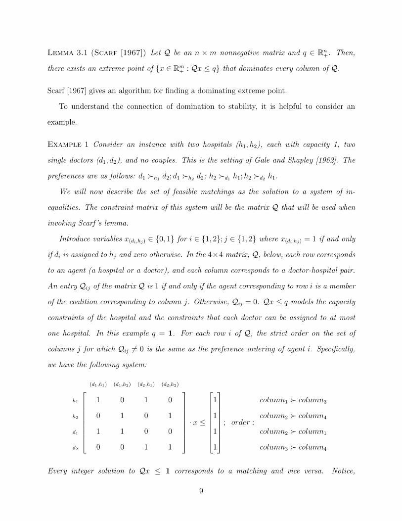
Example 1 Consider an instance with two hospitals (h1, h2), each with capacity 1, two

single doctors (d1, d2), and no couples. This is the setting of Gale and Shapley [1962]. The

preferences are as follows: d1 �h1 d2; d1 �h2 d2; h2 �d1 h1;h2 �d2 h1.

We will now describe the set of feasible matchings as the solution to a system of in-

equalities. The constraint matrix of this system will be the matrix Q that will be used when

invoking Scarf ’s lemma.

Introduce variables x(di,hj) ∈ {0, 1} for i ∈ {1, 2}; j ∈ {1, 2} where x(di,hj) = 1 if and only

if di is assigned to hj and zero otherwise. In the 4×4 matrix, Q, below, each row corresponds

to an agent (a hospital or a doctor), and each column corresponds to a doctor-hospital pair.

An entry Qij of the matrix Q is 1 if and only if the agent corresponding to row i is a member

of the coalition corresponding to column j. Otherwise, Qij = 0. Qx ≤ q models the capacity

constraints of the hospital and the constraints that each doctor can be assigned to at most

one hospital. In this example q = 1. For each row i of Q, the strict order on the set of

columns j for which Qij 6= 0 is the same as the preference ordering of agent i. Specifically,

we have the following system:

(d1,h1) (d1,h2) (d2,h1) (d2,h2)

h1 1 0 1 0

h2 0 1 0 1

d1 1 1 0 0

d2 0 0 1 1

· x ≤

1

1

1

1

; order :

column1 � column3

column2 � column4

column2 � column1

column3 � column4.

Every integer solution to Qx ≤ 1 corresponds to a matching and vice versa. Notice,

9

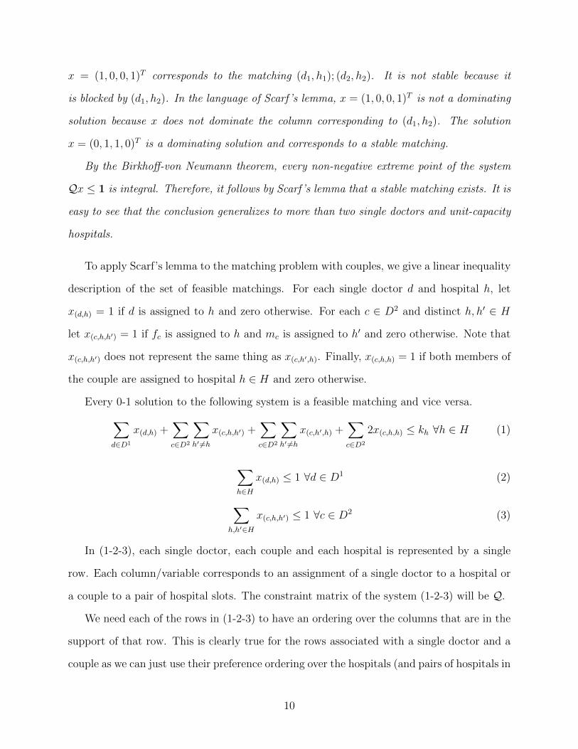
x = (1, 0, 0, 1)T corresponds to the matching (d1, h1); (d2, h2). It is not stable because it

is blocked by (d1, h2). In the language of Scarf ’s lemma, x = (1, 0, 0, 1)T is not a dominating

solution because x does not dominate the column corresponding to (d1, h2). The solution

x = (0, 1, 1, 0)T is a dominating solution and corresponds to a stable matching.

By the Birkhoff-von Neumann theorem, every non-negative extreme point of the system

Qx ≤ 1 is integral. Therefore, it follows by Scarf ’s lemma that a stable matching exists. It is

easy to see that the conclusion generalizes to more than two single doctors and unit-capacity

hospitals.

To apply Scarf’s lemma to the matching problem with couples, we give a linear inequality

description of the set of feasible matchings. For each single doctor d and hospital h, let

x(d,h) = 1 if d is assigned to h and zero otherwise. For each c ∈ D2 and distinct h, h′ ∈ H

let x(c,h,h′) = 1 if fc is assigned to h and mc is assigned to h′ and zero otherwise. Note that

x(c,h,h′) does not represent the same thing as x(c,h′,h). Finally, x(c,h,h) = 1 if both members of

the couple are assigned to hospital h ∈ H and zero otherwise.

Every 0-1 solution to the following system is a feasible matching and vice versa.∑d∈D1

x(d,h) +∑c∈D2

∑h′ 6=h

x(c,h,h′) +∑c∈D2

∑h′ 6=h

x(c,h′,h) +∑c∈D2

2x(c,h,h) ≤ kh ∀h ∈ H (1)

∑h∈H

x(d,h) ≤ 1 ∀d ∈ D1 (2)

∑h,h′∈H

x(c,h,h′) ≤ 1 ∀c ∈ D2 (3)

In (1-2-3), each single doctor, each couple and each hospital is represented by a single

row. Each column/variable corresponds to an assignment of a single doctor to a hospital or

a couple to a pair of hospital slots. The constraint matrix of the system (1-2-3) will be Q.

We need each of the rows in (1-2-3) to have an ordering over the columns that are in the

support of that row. This is clearly true for the rows associated with a single doctor and a

couple as we can just use their preference ordering over the hospitals (and pairs of hospitals in

10

the case of couples). Unlike example 2, an additional difficulty will be to represent a hospital

h’s priority ordering, �h, over individual doctors in terms of an ordering, �∗h, over columns

associated with coalitions involving either a single doctor or a couple and the hospital h.

This is captured in the following definition:

Definition 3.2 Hospital h’s priority ordering over the individual doctors, �h, and the pref-

erences of the couples {�c: c ∈ C} is used to construct a strict ordering, �∗h, over the vari-

ables representing the assignment of a doctor or a couple to at least one position at h–namely,

the variables of the form x(d,h), x(c,hh′), x(c,h′h), and x(c,hh). Denote by x·,h a generic instance

of one of these variables. �∗h is defined as follows.

For each variable x·,h, let d(x) be the doctor assigned to h. If x·,h represents the assignment

of a couple to h, let d(x·,h) be the least preferred (by h) one. For x·,h 6= x′·,h, if d(x·,h) �h

d(x′·,h), then x·,h �∗h x′·,h. If d(x·,h) = d(x′·,h), then x·,h and x′·,h represents two different

assignments of a couple c, in which case, x·,h �∗h x′·,h if and only if x·,h �c x′·,h. For an

example see example 4 in the appendix.

Under the ordering �∗h , we obtain the following result. Its proof is given in Appendix B.

Lemma 3.2 Let x∗ be a dominating solution of (1-2-3). If x∗ is integral, then x∗ is a stable

matching for the matching with couples problem.

If the extreme points of (1-2-3) are integral, then, by Scarf’s lemma, one of these is

dominating. By Lemma 3.2, this matching will be stable. Unfortunately, (1-2-3) is not an

integral polytope. The example below, from Klaus and Klijn [2005], shows that there need

be no integral dominating extreme point when couples are present. This explains the need

for the rounding step in our algorithm discussed in Section 4.13

Example 2 We have two hospitals (h1, h2) each with capacity 1, one couple (d1, d2) and

one single doctor (d3). The preferences of each are listed below:

13 Scarf’s algorithm for finding a dominating extreme point is not guaranteed to find a stable matchingeven if it exists. If the dominating extreme point is integral, it will correspond to a stable matching, otherwisenot. It is an open question whether Scarf’s algorithm can be modified to find a dominating extreme pointthat is integral when it exists.

11

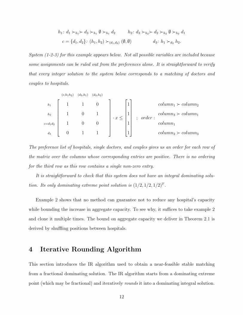
h1: d1 �h1� d3 �h1 ∅ �h1 d2 h2: d3 �h2� d2 �h2 ∅ �h2 d1

c = {d1, d2}: (h1, h2) �(d1,d2) (∅, ∅) d3: h1 �d3 h2.

System (1-2-3) for this example appears below. Not all possible variables are included because

some assignments can be ruled out from the preferences alone. It is straightforward to verify

that every integer solution to the system below corresponds to a matching of doctors and

couples to hospitals.

(c,h1h2) (d3,h1) (d3,h2)

h1 1 1 0

h2 1 0 1

c=d1d2 1 0 0

d3 0 1 1

· x ≤

1

1

1

1

; order :

column1 � column2

column3 � column1

column1

column2 � column3

The preference list of hospitals, single doctors, and couples gives us an order for each row of

the matrix over the columns whose corresponding entries are positive. There is no ordering

for the third row as this row contains a single non-zero entry.

It is straightforward to check that this system does not have an integral dominating solu-

tion. Its only dominating extreme point solution is (1/2, 1/2, 1/2)T .

Example 2 shows that no method can guarantee not to reduce any hospital’s capacity

while bounding the increase in aggregate capacity. To see why, it suffices to take example 2

and clone it multiple times. The bound on aggregate capacity we deliver in Theorem 2.1 is

derived by shuffling positions between hospitals.

4 Iterative Rounding Algorithm

This section introduces the IR algorithm used to obtain a near-feasible stable matching

from a fractional dominating solution. The IR algorithm starts from a dominating extreme

point (which may be fractional) and iteratively rounds it into a dominating integral solution.

12

This will produce a stable matching of doctors to hospitals that may violate the capacity

constraints of some of the hospitals. Our main result shows that the violation is not too

large.

Let x be a dominating extreme point of (1-2-3). Under allocation x, some hospitals

can be under-demanded. However, we can, with the introduction of dummy doctors, assume

without loss that positions at every hospital are fully allocated.14 For economy of exposition,

let H be the constraint matrix associated with hospital constraints (1). Then, (1) can be

expressed as Hx = k.

The IR algorithm will round x into an integral x∗ such that Hx∗ = k∗, where k∗ is close

to k. For the matching corresponding to x∗ to be stable with respect to k∗, we need x∗ to

satisfy the properties in the following lemma whose proof is given in Appendix C.1.

Lemma 4.1 Let x be a fractional dominating extreme point of (1-2-3) and x∗ ≥ 0 be an

integral solution satisfying:

(i). For a single doctor d and a hospital h, if x(d,h) = 0 then x∗(d,h) = 0. Similarly, for a

couple c and hospitals h, h′, if x(c,h,h′) = 0 then x∗(c,h,h′) = 0.

(ii). For a single doctor d, if∑

h x(d,h) = 1, then∑

h x∗(d,h) = 1. Similarly, for any couple c,

if∑

h,h′ x(c,h,h′) = 1, then∑

h,h′ x∗(c,h,h′) = 1.

Let k∗ = Hx∗; then, x∗ is a stable matching with respect to k∗.

Property (i) ensures that the support of x∗ is contained within the support of x and

therefore, x∗ will also be dominating. Property (ii) ensures that if a single doctor or couple

is fully assigned under x, then they are fully assigned under x∗. Both are needed to ensure

that the rounded solution x∗ continues to be a dominating solution with respect to the new

hospital capacities. Recall that in the definition of domination, a zero component of x is

dominated via a binding constraint. Property (ii) ensures that if a constraint corresponding

to a doctor or a couple binds under x, then it continues to bind under x∗.

14See Appendix C.2.

13

The Algorithm: To describe the IR algorithm for our matching problem, let x be a dom-

inating extreme point of (1-2-3), and let D0, D1 be the matrices that correspond to the

constraints of (2)-(3) that are binding, slack under x, respectively. To maintain property (ii)

of Lemma 4.1, x is iteratively rounded into x∗ so that all intermediate solutions satisfy

D0 · x = 1;D1 · x ≤ 1;x ≥ 0. (4)

We maintain D0 · x = 1 so that condition (ii) of Lemma 4.1 holds.

To limit the aggregate capacity of hospitals we impose an additional constraint on ag-

gregate capacity:∑

d,h x(d,h) +∑

c,h,h′ 2x(c,h,h′) ≤∑

h kh. We write this constraint in matrix

form as a · x ≤∑h kh, where a(d,h) = 1; a(c,h,h′) = a(c,h,h) = 2.

Denote by Hh the row vector of H corresponding to h ∈ H. The IR starts with x that

satisfies (2)-(3) as well as the following:

Hh · x = kh for all hospital h and a · x ≤∑h

kh. (5)

The constraints of (5) will gradually be discarded during the execution of the algorithm.

Call a constraint in (5) active if it has not yet been eliminated.

The IR algorithm is described in Figure 1 in which we use the following notation. For a

vector x, denote by dxe the vector whose ith component is dxie. Similarly, bxc is the vector

whose ith component is bxic. Thus, the ith component of dxe − bxc is 1 if the corresponding

component of x is fractional and 0 otherwise.

We use the instance from example 2 to illustrate the IR algorithm.

Example 3 From example 2, we know that x = (1/2, 1/2, 1/2)T is the only dominating

extreme point. The couple is assigned to (h1, h2) with weight 1/2 and the single doctor 3 is

assigned to h1, h2 with weight 1/2, each.

Beginning with x, we see that the constraint corresponding to doctor d3 binds. The con-

straints corresponding to h1, h2 and the aggregate constraint all bind. Each hospital capacity

constraint satisfies the elimination criteria. Eliminate the capacity constraint associated with

h1. The active constraints now consist of the aggregate constraint and the capacity constraint

14

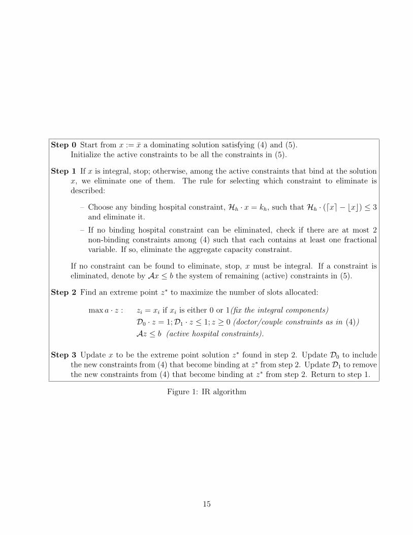
Step 0 Start from x := x a dominating solution satisfying (4) and (5).Initialize the active constraints to be all the constraints in (5).

Step 1 If x is integral, stop; otherwise, among the active constraints that bind at the solutionx, we eliminate one of them. The rule for selecting which constraint to eliminate isdescribed:

– Choose any binding hospital constraint, Hh · x = kh, such that Hh · (dxe − bxc) ≤ 3and eliminate it.

– If no binding hospital constraint can be eliminated, check if there are at most 2non-binding constraints among (4) such that each contains at least one fractionalvariable. If so, eliminate the aggregate capacity constraint.

If no constraint can be found to eliminate, stop, x must be integral. If a constraint iseliminated, denote by Ax ≤ b the system of remaining (active) constraints in (5).

Step 2 Find an extreme point z∗ to maximize the number of slots allocated:

max a · z : zi = xi if xi is either 0 or 1(fix the integral components)

D0 · z = 1;D1 · z ≤ 1; z ≥ 0 (doctor/couple constraints as in (4))

Az ≤ b (active hospital constraints).

Step 3 Update x to be the extreme point solution z∗ found in step 2. Update D0 to includethe new constraints from (4) that become binding at z∗ from step 2. Update D1 to removethe new constraints from (4) that become binding at z∗ from step 2. Return to step 1.

Figure 1: IR algorithm

15

of h2. None of the variables is integral. Thus, in Step 2, we solve the following linear program

to get a new extreme point.

max 2x(c,h1h2) + x(d3,h1) + x(d3,h2)

st : x(d3,h1) + x(d3,h2) = 1 (doctor d3’s constraint to maintain (ii) in Lemma 4.1)

x(c,h1h2) ≤ 1 (constraint for couple c)

x(c,h1h2) + x(d3,h2) = 1 (constraint for hospital h2)

2x(c,h1h2) + x(d3,h1) + x(d3,h2) ≤ 2 (aggregate constraint)

The solution is x(c,h1h2) = 12; x(d3,h1) = 1

2; x(d3,h2) = 1

2.

With this solution, the IR algorithm goes to the next iteration. Hospital h2’s capacity

constraint binds and satisfies the elimination criteria. Eliminate it. In the next iteration we

solve the following linear program.

max 2x(c,h1h2) + x(d3,h1) + x(d3,h2)

st : x(d3,h1) + x(d3,h2) = 1 (doctor d3’s constraint to maintain (ii) in Lemma 4.1)

x(c,h1h2) ≤ 1 (constraint for couple c)

2x(c,h1h2) + x(d3,h1) + x(d3,h2) ≤ 2 (aggregate constraint)

The solution is x(c,h1h2) = 12; x(d3,h1) = 1; x(d3,h2) = 0. Now, variables x(d3,h1) and x(d3,h2)

are integral and fixed. x(c,h1h2) is the only variable, and x(c,h1h2) ≤ 1 is the only constraint.

Solving this, we obtain the final solution x(c,h1h2) = x(d3,h1) = 1; x(d3,h2) = 0. While integral,

it only violates the discarded constraint associated with hospital h1 by exactly 1.

Remark. The decision to eliminate the capacity constraint associated with h1 was arbitrary.

We could have eliminated the constraint corresponding to h2 instead. The resulting solution

would have violated hospital 2’s capacity constraint instead. This flexibility allows one

to prioritize one hospital over another based on the relative “softness” of their capacity

constraints.

16

The IR algorithm can also prioritize hospitals through the choice of objective function in

Step 2 of the algorithm. See Appendix E.2 for a more detailed discussion.

Before we give the proof of Theorem 2.1, we provide some intuition. Starting with a

dominating extreme point, x∗, say, we will round it into an integral dominating vector. Ev-

ery component of x∗ that is rounded up to 1, will lead to a violation of a capacity constraint.

The extent of the violation for a given hospital h, will depend on the number of fractional of

components of x∗ associated with h. The essence of the proof is that there must be a hospital

with only a small number, 2 in fact, of fractional components of x∗ associated with it. How

can that be? If it were not so, every hospital capacity constraint must contain within its

support at least 3 fractional components of x∗. However, each component of x∗ appears it at

most two hospital constraints. The nub of the argument is that there are simply not enough

fractional components to go around.

Proof of Theorem 2.1. We show that the IR algorithm generates x∗ satisfying Lemma 4.1

and that the new hospital capacity vector k∗ is not too far from k. First, in Step 2, a variable

of x at zero remains at zero throughout the algorithm. Hence, the first property in Lemma 4.1

is maintained. Second, in Step 2, we always maintain the doctor/couple constraints (4), so

the second property in Lemma 4.1 is also satisfied.

At Step 2, because the current vector x is feasible for this linear program, the optimal

solution z satisfies a · z ≥ a · x. This guarantees that we never reduce the number of slots

available. If the aggregate constraint is never eliminated during the course of the algorithm,

then, trivially, the aggregate capacity never increases. If the aggregate constraint is elimi-

nated, it means at most two constraints from (4) do not bind and contain fractional variables.

Each of these constraints corresponds to either a single doctor or a couple. These are the

only single doctors or couples not yet fully allocated. Collectively they would occupy at

most 4 slots. Hence, in the worst case we will need to add 4 additional slots to accommodate

them.

17

We argue that the error bound for each hospital is at most 2. Consider, first, any hospital

whose corresponding hospital constraint Hh · x = kh was eliminated at some stage during

the execution of the algorithm. Therefore, Hh · (dxe − bxc) ≤ 3. This implies

Hh · (dxe − x) +Hh · (x− bxc) ≤ 3. (6)

We have two cases. First, if either Hh · (dxe− x) or Hh · (x−bxc) is 0, then all the variables

that appear in this constraint are integral. According to the algorithm, these variables will

be fixed at their current values. Thus, the corresponding hospital constraint will never be

violated.

In the second case, both Hh · (dxe − x) and Hh · (x − bxc) are strictly greater than 0.

Because Hh · x = kh, it follows that Hh · x is integral. As Hh · dxe, and Hh · bxc are integral

as well, Hh · (dxe − x) ≥ 1 and Hh · (x − bxc) ≥ 1. But because of (6), this would imply

that Hh · (dxe − x) = Hh · dxe − kh ≤ 2 and Hh · (x − bxc) = kh − Hh · bxc ≤ 2. Thus,

after eliminating this hospital constraint, at worst, we might violate its right hand side by

at most 2.

To verify that the algorithm terminates, we must show that at Step 1, if no integral

solution is found, there is a binding constraint to be eliminated. Suppose the current solution

is x, and the algorithm has not yet terminated. If no binding hospital constraints remain,

x is an extreme point of (4) (equivalently (2), (3)). The corresponding constraint matrix is

totally unimodular (see Vohra [2005] for a definition) because every variable appears in at

most one constraint, x is integral. This contradicts the fact that the algorithm has not yet

terminated. Hence, there must be at least one active binding constraint in (5) that satisfies

the condition for elimination. If none, we use a counting argument to show that this would

contradict the extreme point property of x. This argument is given in Appendix D.

18

5 Conclusion

A key goal in the design of centralized matching markets is to eliminate the incentive for par-

ticipants to contract outside of the market. This is formalized as stability and is considered

crucial for the long-term sustainability of a market. In the presence of complementarities,

stable matchings need not exist. Others have responded to this challenge by restricting pref-

erences or weakening the notion of stability. We, instead, weaken “feasibility” and establish

the existence of near-feasible stable matchings in the presence of complementarities.

Acknowledgements

We thank Nicholas Arnosti, Eric Budish, Fuhito Kojima, Ben Roth and the associate editor

and anonymous referees for their useful comments. Peter Biro was particularly helpful with

extensive suggestions.

References

R. Aharoni and T. Fleiner. On a lemma of Scarf. Journal of Combinatorial Theory, Series

B, 87:72—80, 2003.

R. Aharoni and R. Holzman. Fractional kernels in digraphs. Journal of Combinatorial

Theory, Series B, 73(1):1–6, 1998.

I. Ashlagi, M. Braverman, and A. Hassidim. Stability in large matching markets with com-

plementarities. Operations Research, 62(4):713–732, 2014.

P. Biro and T. Fleiner. Fractional solutions for capacitated ntu-games, with applications to

stable matchings. Discrete Optimization, 22:241–254, Dec. 2016.

P. Biro and F. Klijn. Matching With Couples: A Multidisciplinary Survey. International

Game Theory Review, 15(02), 2013.

P. Biro, T. Fleiner, and R. Irving. Matching couples with scarf’s algorithm. Proc. 8th

Hungarian-Japanese Symposium on Discrete Mathematics and its Applications, 2013.

19

E. Budish. The combinatorial assignment problem: Approximate competitive equilibrium

from equal incomes. Journal of Political Economy, 119(6):1061 – 1103, 2011.

D. Cantala. Matching markets: the particular case of couples. Economics Bulletin, 3(45):

1–11, 2004.

B. C. Dean, M. X. Goemans, and N. Immorlica. The unsplittable stable marriage problem. In

Fourth IFIP International Conference on Theoretical Computer Science-TCS 2006, pages

65–75. Springer US, 2006.

T. Fleiner. A fixed-point approach to stable matchings and some applications. Mathematics

of Operations Research, 28(1):103–126, Feb. 2003.

D. Gale and L. S. Shapley. College Admissions and the Stability of Marriage. The American

Mathematical Monthly, 69(1):9–15, 1962.

J. W. Hatfield and F. Kojima. Substitutes and stability for matching with contracts. Journal

of Economic Theory, 145(5):1704–1723, 2010.

J. W. Hatfield and P. R. Milgrom. Matching with Contracts. American Economic Review,

95(4):913–935, September 2005.

Z. Jiang and G. Tan. Matching with couples: Semi-stability and algorithm. 2014.

S. Kintali. Scarf is PPAD-complete. CoRR, abs/0812.1601, 2008.

T. Kiraly and J. Pap. Kernels, stable matchings, and scarf’s lemma. Working paper, Egervary

Research Group, TR-2008-13, 2008.

B. Klaus and F. Klijn. Stable matchings and preferences of couples. Journal of Economic

Theory, 121(1):75–106, 2005.

F. Klijn and J. Masso. Weak stability and a bargaining set for the marriage model. Games

and Economic Behavior, 42:91–100, 2003.

F. Kojima, P. A. Pathak, and A. E. Roth. Matching with couples: Stability and incentives

in large markets. The Quarterly Journal of Economics, 128(4):1585–1632, 2013.

L.-C. Lau, R. Ravi, and M. Singh. Iterative Methods in Combinatorial Optimization. Cam-

bridge University Press, New York, NY, USA, 2011.

D. Manlove, I. McBride, and J. Trimble. “Almost-stable” matchings in the hospi-

tals/residents problem with couples. 2016.

20

T. Nguyen, A. Peivandi, and R. Vohra. Assignment problems with complementarities. Jour-

nal of Economic Theory, 165:209–241, 2016.

M. Ostrovsky. Stability in supply chain networks. American Economic Review, 98(3):897–

923, 2008.

M. Pycia. Stability and preference alignment in matching and coalition formation. Econo-

metrica, 80(1):323–362, 2012. ISSN 1468-0262.

A. Roth and M. Sotomayor. Two-Sided Matching: A Study in Game-Theoretic Modeling

and Analysis. Econometric Society Monographs. Cambridge University Press, 1992. ISBN

9780521437882.

A. E. Roth. The evolution of the labor market for medical interns and residents: A case

study in game theory. Journal of Political Economy, 92(6):pp. 991–1016, 1984.

A. E. Roth and E. Peranson. The redesign of the matching market for american physicians:

Some engineering aspects of economic design. American Economic Review, 89(4):748–780,

1999.

H. E. Scarf. An elementary proof of a theorem on the core of an n person game. 1965.

H. E. Scarf. The core of an n− person game. Econometrica, 35(1):pp. 50–69, 1967.

J. Sethuraman, C.-P. Teo, and L. Qian. Many-to-one stable matching: Geometry and fair-

ness. Mathematics of Operations Research, 31(3):581–596, 2006.

R. Vohra. Advanced Mathematical Economics. Routledge, New York, NY, USA, 2005.

Appendix

A Stability

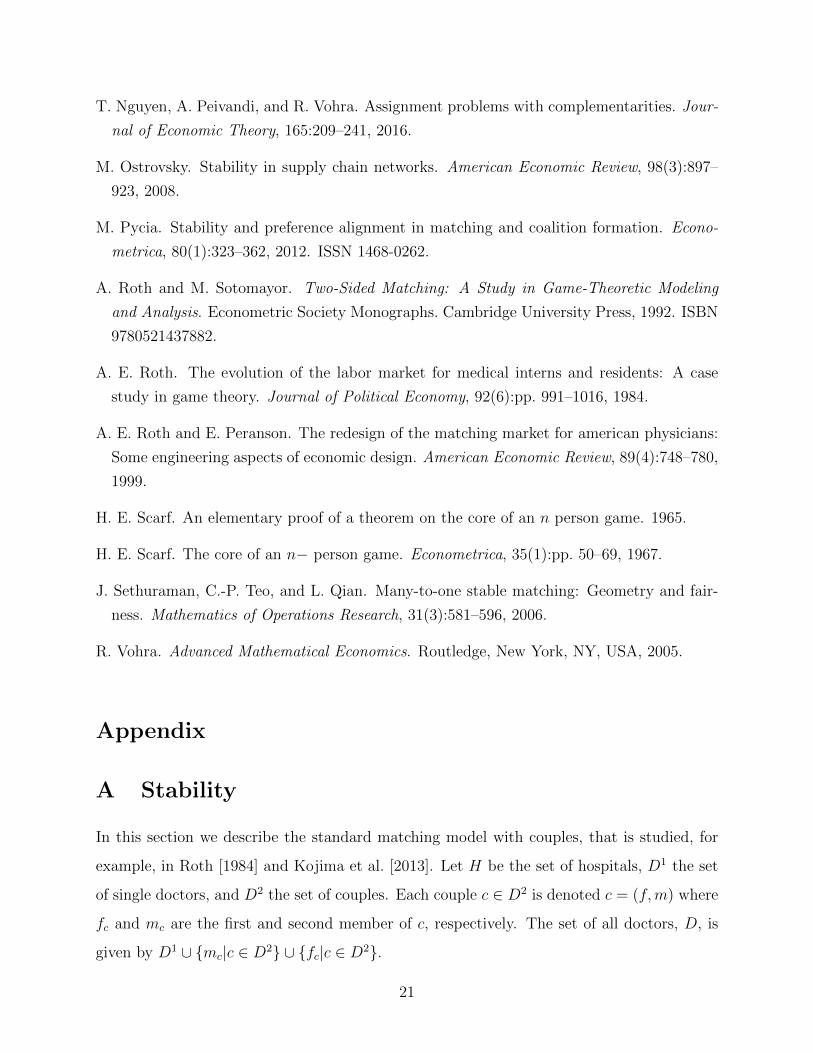
In this section we describe the standard matching model with couples, that is studied, for

example, in Roth [1984] and Kojima et al. [2013]. Let H be the set of hospitals, D1 the set

of single doctors, and D2 the set of couples. Each couple c ∈ D2 is denoted c = (f,m) where

fc and mc are the first and second member of c, respectively. The set of all doctors, D, is

given by D1 ∪ {mc|c ∈ D2} ∪ {fc|c ∈ D2}.

21

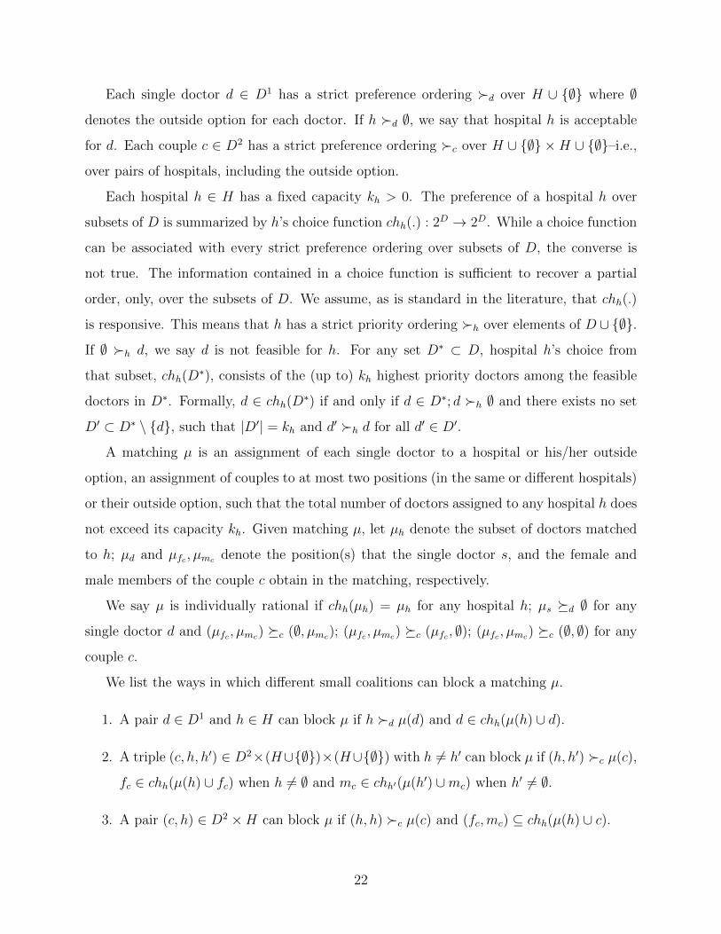
Each single doctor d ∈ D1 has a strict preference ordering �d over H ∪ {∅} where ∅denotes the outside option for each doctor. If h �d ∅, we say that hospital h is acceptable

for d. Each couple c ∈ D2 has a strict preference ordering �c over H ∪ {∅} ×H ∪ {∅}–i.e.,

over pairs of hospitals, including the outside option.

Each hospital h ∈ H has a fixed capacity kh > 0. The preference of a hospital h over

subsets of D is summarized by h’s choice function chh(.) : 2D → 2D. While a choice function

can be associated with every strict preference ordering over subsets of D, the converse is

not true. The information contained in a choice function is sufficient to recover a partial

order, only, over the subsets of D. We assume, as is standard in the literature, that chh(.)

is responsive. This means that h has a strict priority ordering �h over elements of D ∪ {∅}.If ∅ �h d, we say d is not feasible for h. For any set D∗ ⊂ D, hospital h’s choice from

that subset, chh(D∗), consists of the (up to) kh highest priority doctors among the feasible

doctors in D∗. Formally, d ∈ chh(D∗) if and only if d ∈ D∗; d �h ∅ and there exists no set

D′ ⊂ D∗ \ {d}, such that |D′| = kh and d′ �h d for all d′ ∈ D′.A matching µ is an assignment of each single doctor to a hospital or his/her outside

option, an assignment of couples to at most two positions (in the same or different hospitals)

or their outside option, such that the total number of doctors assigned to any hospital h does

not exceed its capacity kh. Given matching µ, let µh denote the subset of doctors matched

to h; µd and µfc , µmc denote the position(s) that the single doctor s, and the female and

male members of the couple c obtain in the matching, respectively.

We say µ is individually rational if chh(µh) = µh for any hospital h; µs �d ∅ for any

single doctor d and (µfc , µmc) �c (∅, µmc); (µfc , µmc) �c (µfc , ∅); (µfc , µmc) �c (∅, ∅) for any

couple c.

We list the ways in which different small coalitions can block a matching µ.

1. A pair d ∈ D1 and h ∈ H can block µ if h �d µ(d) and d ∈ chh(µ(h) ∪ d).

2. A triple (c, h, h′) ∈ D2×(H∪{∅})×(H∪{∅}) with h 6= h′ can block µ if (h, h′) �c µ(c),

fc ∈ chh(µ(h) ∪ fc) when h 6= ∅ and mc ∈ chh′(µ(h′) ∪mc) when h′ 6= ∅.

3. A pair (c, h) ∈ D2 ×H can block µ if (h, h) �c µ(c) and (fc,mc) ⊆ chh(µ(h) ∪ c).

22

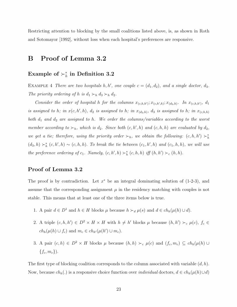
Restricting attention to blocking by the small coalitions listed above, is, as shown in Roth

and Sotomayor [1992], without loss when each hospital’s preferences are responsive.

B Proof of Lemma 3.2

Example of �∗h in Definition 3.2

Example 4 There are two hospitals h, h′, one couple c = (d1, d2), and a single doctor, d3.

The priority ordering of h is d1 �h d3 �h d2.

Consider the order of hospital h for the columns x(c,h,h′);x(c,h′,h);x(d3,h). In x(c,h,h′), d1

is assigned to h; in x(c, h′, h), d2 is assigned to h; in x(d3,h), d3 is assigned to h; in x(c,h,h)

both d1 and d2 are assigned to h. We order the columns/variables according to the worst

member according to �h, which is d2. Since both (c, h′, h) and (c, h, h) are evaluated by d2,

we get a tie; therefore, using the priority order �h, we obtain the following: (c, h, h′) �∗h(d3, h) �∗h (c, h′, h) ∼ (c, h, h). To break the tie between (c1, h

′, h) and (c1, h, h), we will use

the preference ordering of c1. Namely, (c, h′, h) �∗h (c, h, h) iff (h, h′) �c (h, h).

Proof of Lemma 3.2

The proof is by contradiction. Let x∗ be an integral dominating solution of (1-2-3), and

assume that the corresponding assignment µ in the residency matching with couples is not

stable. This means that at least one of the three items below is true.

1. A pair d ∈ D1 and h ∈ H blocks µ because h �d µ(s) and d ∈ chh(µ(h) ∪ d).

2. A triple (c, h, h′) ∈ D2 × H × H with h 6= h′ blocks µ because (h, h′) �c µ(c), fc ∈chh(µ(h) ∪ fc) and mc ∈ chh′(µ(h′) ∪mc).

3. A pair (c, h) ∈ D2 × H blocks µ because (h, h) �c µ(c) and (fc,mc) ⊆ chh(µ(h) ∪{fc,mc}).

The first type of blocking coalition corresponds to the column associated with variable (d, h).

Now, because chh(.) is a responsive choice function over individual doctors, d ∈ chh(µ(h)∪d)

23

implies that d is among the best kh candidates among µ(h) ∪ d. Therefore, x∗ does not

dominate column (d, h): this is a contradiction because x∗ is a dominating solution.

The second type of blocking coalition corresponds to column (c, h, h′). Following the

same argument, the blocking coalition implies that fc is among the best kh candidates among

µ(h)∪fc (similar for mc and h′.) Together with the tie-breaking rule of �∗h This implies that

x∗ does not dominate the column (c, h, h′).

In the third type of blocking coalition, the pair (fc,mc) and a hospital h correspond to

a column (c, h, h). Because (fc,mc) ⊆ chh(µ(h) ∪ c), both fc and mc are among the kh best

candidates, even when we consider the order �∗ for the columns, because both members

are still ranked highly among µh ∪ {fc,mc}. Together with the tie-breaking rule of �∗h, this

implies that x∗ does not block column (c, h, h).

C Maintaining Stability in Rounding

C.1 Proof of Lemma 4.1

First of all, x∗ is a feasible matching with respect to k∗. Using the fact that x dominates

all columns of Q, we show that under the new capacity vector k∗, x∗ dominates all columns

of Q.

Consider the column associated with the assignment of couple c0 to hospital h1 and h2,

(c0, h1, h2). (A similar argument will apply to the other columns). x dominates (c0, h1, h2)

either at the constraint corresponding to c0 or at h1 ∈ H or at h2 ∈ H.

Suppose first x dominates (c0, h1, h2) at c0. Then∑

h,h′ x(c0,h,h′) = 1, and couple c0 does

not like the allocation h1, h2 strictly more than any of the assignments that they obtained

under x. Now because x∗ is a 0− 1 vector rounded from x that satisfies Lemma 4.1:

(i.) x∗(c0,h,h′) > 0 ⇒ x(c0,h,h′) > 0

(ii.)∑

h,h′ x(c0,h,h′) = 1 ⇒ ∑h,h′ x∗(c0,h,h′) = 1.

These imply that c0 (weakly) prefers the assignments that they gets in x∗ more than (h1, h2)

(we use “weakly prefers” because it is possible that x∗(c0,h1,h2)= 1).

24

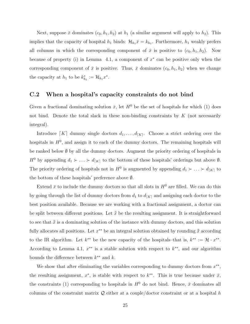
Next, suppose x dominates (c0, h1, h2) at h1 (a similar argument will apply to h2). This

implies that the capacity of hospital h1 binds: Hh1x = kh1 . Furthermore, h1 weakly prefers

all columns in which the corresponding component of x is positive to (c0, h1, h2). Now

because of property (i) in Lemma 4.1, a component of x∗ can be positive only when the

corresponding component of x is positive. Thus, x dominates (c0, h1, h2) when we change

the capacity at h1 to be k∗h1:= Hh1x

∗.

C.2 When a hospital’s capacity constraints do not bind

Given a fractional dominating solution x, let H0 be the set of hospitals for which (1) does

not bind. Denote the total slack in these non-binding constraints by K (not necessarily

integral).

Introduce dKe dummy single doctors d1, . . . , ddKe. Choose a strict ordering over the

hospitals in H0, and assign it to each of the dummy doctors. The remaining hospitals will

be ranked below ∅ by all the dummy doctors. Augment the priority ordering of hospitals in

H0 by appending d1 � . . . � ddKe to the bottom of these hospitals’ orderings but above ∅.The priority ordering of hospitals not in H0 is augmented by appending d1 � . . . � ddKe to

the bottom of these hospitals’ preference above ∅.Extend x to include the dummy doctors so that all slots in H0 are filled. We can do this

by going through the list of dummy doctors from d1 to ddKe and assigning each doctor to the

best position available. Because we are working with a fractional assignment, a doctor can

be split between different positions. Let ¯x be the resulting assignment. It is straightforward

to see that ¯x is a dominating solution of the instance with dummy doctors, and this solution

fully allocates all positions. Let x∗∗ be an integral solution obtained by rounding ¯x according

to the IR algorithm. Let k∗∗ be the new capacity of the hospitals–that is, k∗∗ := H · x∗∗.According to Lemma 4.1, x∗∗ is a stable solution with respect to k∗∗, and our algorithm

bounds the difference between k∗∗ and k.

We show that after eliminating the variables corresponding to dummy doctors from x∗∗,

the resulting assignment, x∗, is stable with respect to k∗∗. This is true because under x,

the constraints (1) corresponding to hospitals in H0 do not bind. Hence, x dominates all

columns of the constraint matrix Q either at a couple/doctor constraint or at a hospital h

25

constraint where h /∈ H0. As dummy doctors are never assigned to hospitals outside of H0,

it follows that for all h /∈ H0, Hh · x∗∗ = Hh · x∗. Hence,

k∗∗h = Hh · x∗∗ = Hh · x∗ = k∗ for h /∈ H0.

With these observations, and following the same argument as in Section C.1, we obtain that

x∗ is stable with respect to k∗∗.

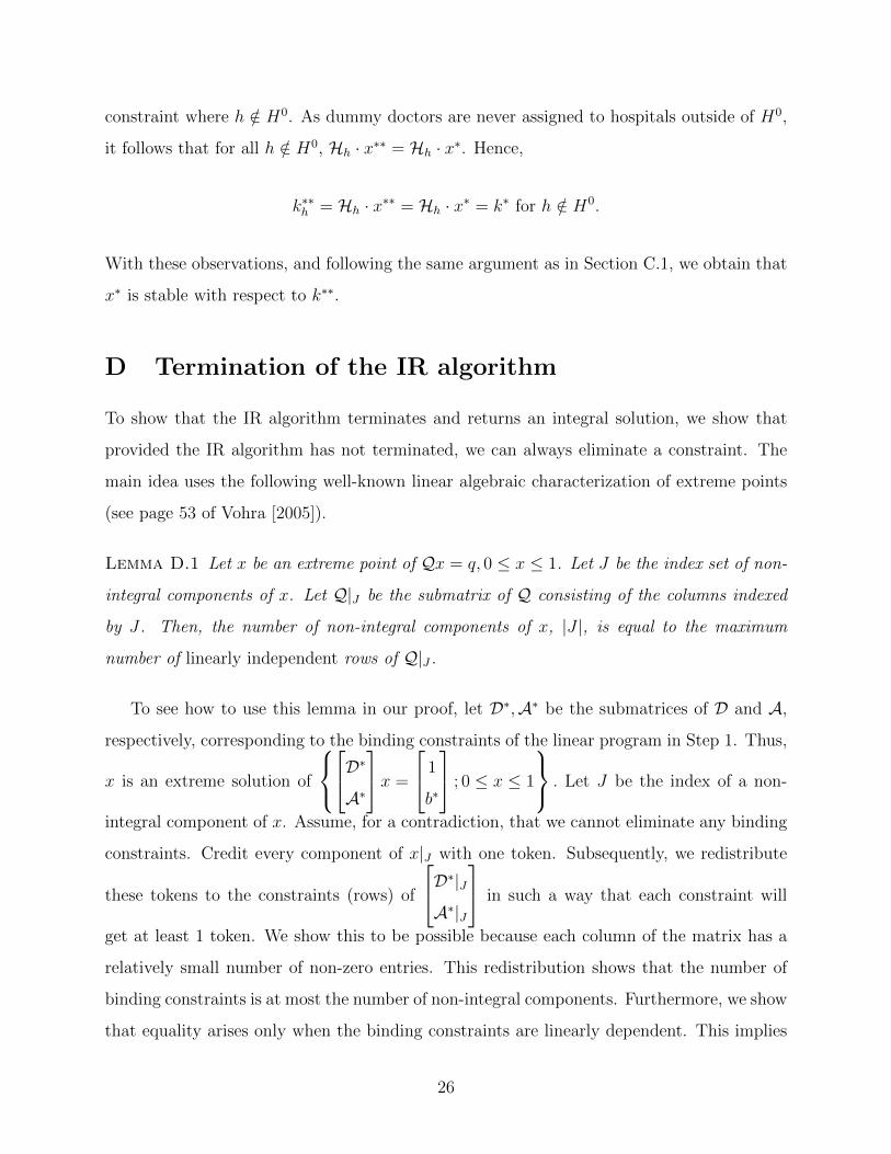
D Termination of the IR algorithm

To show that the IR algorithm terminates and returns an integral solution, we show that

provided the IR algorithm has not terminated, we can always eliminate a constraint. The

main idea uses the following well-known linear algebraic characterization of extreme points

(see page 53 of Vohra [2005]).

Lemma D.1 Let x be an extreme point of Qx = q, 0 ≤ x ≤ 1. Let J be the index set of non-

integral components of x. Let Q|J be the submatrix of Q consisting of the columns indexed

by J . Then, the number of non-integral components of x, |J |, is equal to the maximum

number of linearly independent rows of Q|J .

To see how to use this lemma in our proof, let D∗,A∗ be the submatrices of D and A,

respectively, corresponding to the binding constraints of the linear program in Step 1. Thus,

x is an extreme solution of

D∗A∗

x =

1

b∗

; 0 ≤ x ≤ 1

. Let J be the index of a non-

integral component of x. Assume, for a contradiction, that we cannot eliminate any binding

constraints. Credit every component of x|J with one token. Subsequently, we redistribute

these tokens to the constraints (rows) of

D∗|JA∗|J

in such a way that each constraint will

get at least 1 token. We show this to be possible because each column of the matrix has a

relatively small number of non-zero entries. This redistribution shows that the number of

binding constraints is at most the number of non-integral components. Furthermore, we show

that equality arises only when the binding constraints are linearly dependent. This implies

26

that the maximum number of linearly independent constraints is less than the number of

non-integral components, which contradicts Lemma D.1.

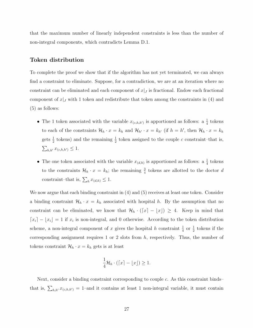
Token distribution

To complete the proof we show that if the algorithm has not yet terminated, we can always

find a constraint to eliminate. Suppose, for a contradiction, we are at an iteration where no

constraint can be eliminated and each component of x|J is fractional. Endow each fractional

component of x|J with 1 token and redistribute that token among the constraints in (4) and

(5) as follows:

• The 1 token associated with the variable x(c,h,h′) is apportioned as follows: a 14

tokens

to each of the constraints Hh · x = kh and Hh′ · x = kh′ (if h = h′, then Hh · x = kh

gets 12

tokens) and the remaining 12

token assigned to the couple c constraint–that is,∑h,h′ x(c,h,h′) ≤ 1.

• The one token associated with the variable x(d,h) is apportioned as follows: a 14

tokens

to the constraints Hh · x = kh; the remaining 34

tokens are allotted to the doctor d

constraint–that is,∑

h x(d,h) ≤ 1.

We now argue that each binding constraint in (4) and (5) receives at least one token. Consider

a binding constraint Hh · x = kh associated with hospital h. By the assumption that no

constraint can be eliminated, we know that Hh · (dxe − bxc) ≥ 4. Keep in mind that

dxie − bxic = 1 if xi is non-integral, and 0 otherwise. According to the token distribution

scheme, a non-integral component of x gives the hospital h constraint 14

or 12

tokens if the

corresponding assignment requires 1 or 2 slots from h, respectively. Thus, the number of

tokens constraint Hh · x = kh gets is at least

1

4Hh · (dxe − bxc) ≥ 1.

Next, consider a binding constraint corresponding to couple c. As this constraint binds–

that is,∑

h,h′ x(c,h,h′) = 1–and it contains at least 1 non-integral variable, it must contain

27

at least 2. Each of the fractional variables contributes 12

a token, thus this constraint also

obtains at least 1 token.

Similarly, for the constraint corresponding to a single doctor d. If this constraint binds

and contains at least one non-integral variable, it must contains at least 2. Therefore, it also

gets at least 2× 34≥ 1 token.

The total number of tokens distributed cannot exceed the number of fractional compo-

nents of x|J which is |J |. The total number of tokens received by binding constraints in

(4) and (5) is at least the number of such binding constraints, |J | − 1. This is because the

aggregate capacity constraint may bind. We have two cases.

Case 1: The aggregate capacity constraint has not yet been eliminated.

We know that the total number of tokens allocated to binding constraints in (4) and (5) is

at least |J | − 1. Because the aggregate constraint has not yet been eliminated, there are

at least three non binding doctor/ couple constraints that contain fractional variables. Ac-

cording to the token distribution scheme, we gave to these constraints at least 3× 12

tokens.

Hence, the total number of tokens assigned to constraints in (4) and (5), binding or not, is

at least |J |+ 12. This exceeds the the total number of tokens to be distributed, a contradiction.

Case 2: The aggregate constraint was eliminated at some earlier iteration.

By the extreme point property of x|J , the |J | binding constraints belong to (4) and (5). Each

one of the binding constraint receives at least one token. Hence, none can receive strictly

more than one token. This means no constraint in (2) can bind. Similarly, no non-binding

constraint can receive any tokens. Hence, in x|J , all variables associated with single doctors

take the value zero. Furthermore, if x(c, h, h′) > 0, the capacity constraints associated with

h and h′ must bind. Hence, if we add up the binding constraints in (3) we get the sum of

the binding constraints in (1). This violates the assumption of linear independence.

28

D.1 Tightness

We outline why the token argument we used cannot be modified to give an improved bound.

We will allow the quantity of tokens allocated to hospital h to depend on h.15 For each

hospital h let rh = Hh · (dxe − bxc). As before, suppose we are at an iteration where no

constraint can be eliminated and each component of x|J is fractional. Endow each fractional

component of x|J with 1 token and redistribute the tokens among the constraints in (1-2-3)

as follows:

• The 1 token associated with the variable x(c,h,h′) is apportioned as follows: 1rh

tokens

to each of the constraints Hh ·x = kh and Hh′ ·x = kh′ (if h = h′, then Hh ·x = kh gets

2rh

tokens) and the remaining 1− 2rh

token assigned to the couple c constraint–that is,∑h,h′ x(c,h,h′) ≤ 1.

• The 1 token associated with the variable x(d,h) is apportioned as follows: 1rh

tokens to

the constraints Hh · x = kh; the remaining 1 − 1rh

tokens are allotted to the doctor d

constraint–that is,∑

h x(d,h) ≤ 1.

It is straightforward to see that the number of tokens allocated to each hospital h is at

leastHh · (dxe − bxc)

rh= 1.

Now, consider the number of tokens allocated to a single doctor d constraint. There must be

at least two hospitals h and h′ such that x(d, h), x(d, h′) > 0. Hence, the number of tokens

allocated to this constraint is at least 1 − 1rh

+ 1 − 1rh′. We need this sum to be at least 1.

Hence, rh, rh′ ≥ 2. A similar argument for a couples, c, constraint requires that

1− 2

rh+ 1− 2

rh′≥ 1 ⇒ rh, rh′ ≥ 4.

Hence, for our token argument to work we need rh ≥ 4 for all hospitals h which is precisely

what we have assumed.

15The same conclusion will be reached even if we allow the quantity of tokens to depend on both thehospital and the identity of the doctors.

29

E Additional Results

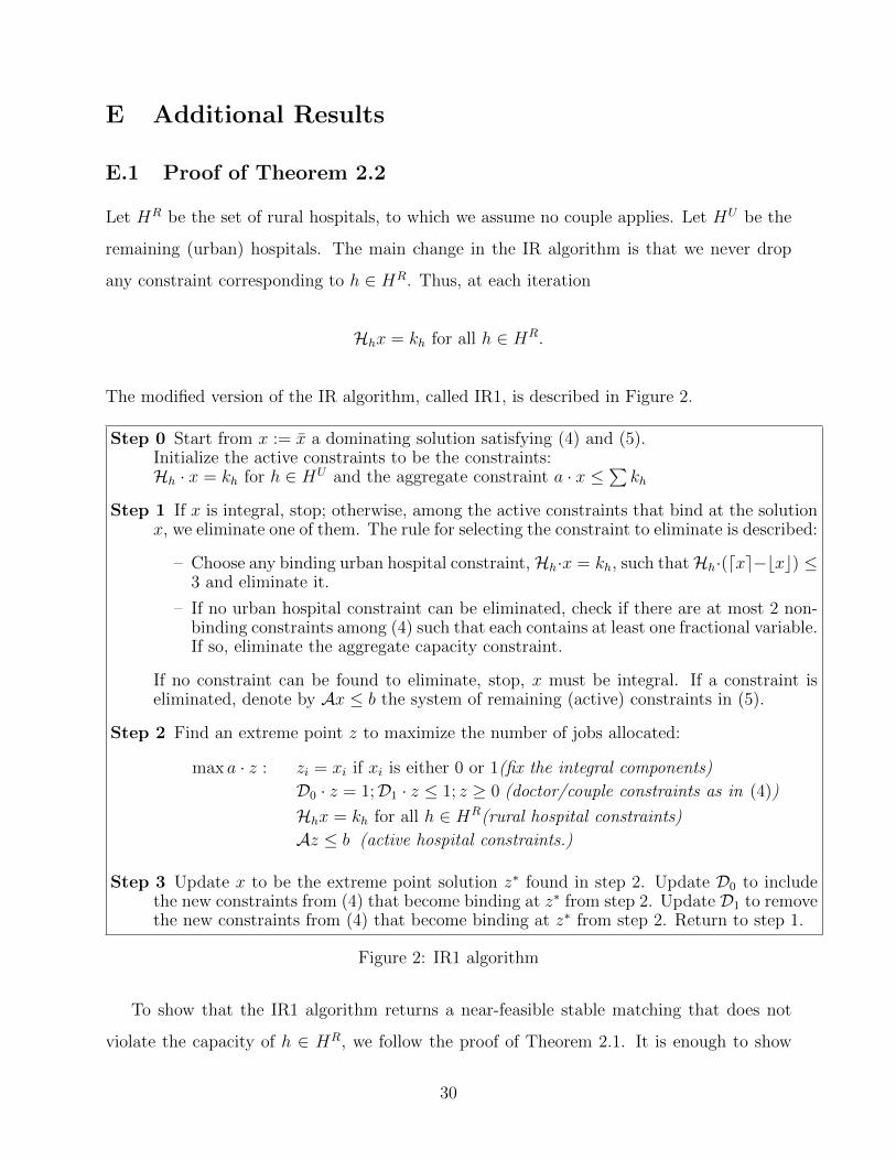
E.1 Proof of Theorem 2.2

Let HR be the set of rural hospitals, to which we assume no couple applies. Let HU be the

remaining (urban) hospitals. The main change in the IR algorithm is that we never drop

any constraint corresponding to h ∈ HR. Thus, at each iteration

Hhx = kh for all h ∈ HR.

The modified version of the IR algorithm, called IR1, is described in Figure 2.

Step 0 Start from x := x a dominating solution satisfying (4) and (5).Initialize the active constraints to be the constraints:Hh · x = kh for h ∈ HU and the aggregate constraint a · x ≤∑

kh

Step 1 If x is integral, stop; otherwise, among the active constraints that bind at the solutionx, we eliminate one of them. The rule for selecting the constraint to eliminate is described:

– Choose any binding urban hospital constraint,Hh·x = kh, such thatHh·(dxe−bxc) ≤3 and eliminate it.

– If no urban hospital constraint can be eliminated, check if there are at most 2 non-binding constraints among (4) such that each contains at least one fractional variable.If so, eliminate the aggregate capacity constraint.

If no constraint can be found to eliminate, stop, x must be integral. If a constraint iseliminated, denote by Ax ≤ b the system of remaining (active) constraints in (5).

Step 2 Find an extreme point z to maximize the number of jobs allocated:

max a · z : zi = xi if xi is either 0 or 1(fix the integral components)

D0 · z = 1;D1 · z ≤ 1; z ≥ 0 (doctor/couple constraints as in (4))

Hhx = kh for all h ∈ HR(rural hospital constraints)

Az ≤ b (active hospital constraints.)

Step 3 Update x to be the extreme point solution z∗ found in step 2. Update D0 to includethe new constraints from (4) that become binding at z∗ from step 2. Update D1 to removethe new constraints from (4) that become binding at z∗ from step 2. Return to step 1.

Figure 2: IR1 algorithm

To show that the IR1 algorithm returns a near-feasible stable matching that does not

violate the capacity of h ∈ HR, we follow the proof of Theorem 2.1. It is enough to show

30

that if IR1 algorithm has not terminated, we can always find an active constraint to delete.

First, because the IR1 algorithm always maintains a solution satisfying the capacity

constraints of rural hospitals, the aggregate constraint can be rewritten in terms of urban

hospitals only. Namely,

∑d,h:h∈HU

x(d,h) +∑

c,h,h′:h,h′∈HU

2x(c,h,h′) ≤∑h∈HU

kh.

Absent from this constraint is any variable x(c,h,h′) where among the pair (h, h′), one is

urban and the other is rural because of our assumption that only single doctors apply to

rural hospitals.

Second, we modify the token distribution scheme by changing how the token associated

with x(d,h) for h ∈ HR is allocated. Namely, assign 12

a token to the constraint Hh · x = kh;

the remaining 1/2 token is given to the doctor d constraint–that is,∑

h x(d,h) ≤ 1. For the

other variables, the token distribution remains the same as in Section D.

Each urban hospital constraint receives at least 1 token. To see why, observe that if a

hospital constraint contains a non-integral variable, it must contain at least two of them.

Each non-integral variable contributes 1/2 a token to the relevant constraint. Thus, the

relevant constraint obtains at least 1 token.

Each couple constraint has at least two non-integral variables or none. When none, we

can ignore this constraint because it does not affect any non-integral variables. As before,

the number of tokens allocated to a couple constraint is at least 1.

Each fractional variable in in a single doctor constraint contributes either 1/2 or 3/4 of

a token depending on whether the corresponding hospital is rural or urban. Thus, such a

constraint also receives at least 1 token and strictly more than that if one of the variables is

associated with an urban hospital.

Hence, as in case 1 in Section D, we can always eliminate one active constraint if the

IR1 algorithm has not terminated. When there are no active constraints left (as in case 2

of Section D), the remaining constraints and variables are associated with the single doctors

and rural hospitals only. This corresponds to the standard linear program of a many-to-one

matching without couples. An extreme point of this linear program is integral.

31

E.2 Using different objective functions to prioritize hospitals

The IR algorithm described in Figure 1 uses an objective function, a · x, to maximize the

number of jobs allocated. Termination of the IR algorithm does not depend on this specific

choice of objective function. The IR algorithm works for any linear objective function, c · x.

This can be used to reflect the fact that assigning extra slots to one hospital may be cheaper

than allocating them to another.

In particular, replacing max a·x with any linear objective function c·x, the IR algorithm in

Figure 1, starting from the fractional stable matching x, will terminate in a 2-feasible stable

matching in which the aggregate capacity does not increase by more than 4. Furthermore,

c · x∗ ≥ c · x.

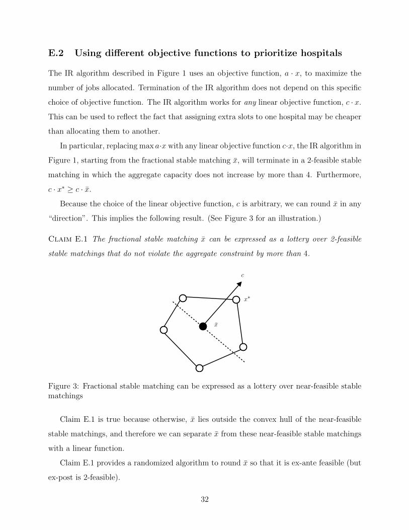
Because the choice of the linear objective function, c is arbitrary, we can round x in any

“direction”. This implies the following result. (See Figure 3 for an illustration.)

Claim E.1 The fractional stable matching x can be expressed as a lottery over 2-feasible

stable matchings that do not violate the aggregate constraint by more than 4.

c

x

x∗

Figure 3: Fractional stable matching can be expressed as a lottery over near-feasible stablematchings

Claim E.1 is true because otherwise, x lies outside the convex hull of the near-feasible

stable matchings, and therefore we can separate x from these near-feasible stable matchings

with a linear function.

Claim E.1 provides a randomized algorithm to round x so that it is ex-ante feasible (but

ex-post is 2-feasible).

32