i

NEAR EAST UNIVERSITY

GRADUATE SCHOOL OF APPLIED

SCIENCES

INCREASING POWER SYSTEM LINE SECURITY

BY USING LOAD MANGEMENT AND

SENSITIVITY ANALYSIS

Saffet AŞIKSOY

Master Thesis

Department of Electrical and Electronic Engineering

Nicosia - 2010

ii

ACKNOWLEDGEMENTS

I would like to thank my supervisor Assoc. Prof. Dr Murat Fahrioğlu for his guidance,

supervision, support and encouragement through this work.

I am also very grateful to Prof. Dr. Şenol BEKTAS and Prof. Dr. Fahreddin M.

SADIKOĞLU for their help and support in every stage of my study.

Special thanks go to my dear wife and my parents, who have encouraged and supported

me through all these years.

iii

To my dear wife Gülsüm and my daughter Azra

iv

ABSTRACT

In any power system today line flows play an integral part. System security is very

much dependent on all the lines being healthy and able to transmit power from

generating stations all the way to the consumers. As the conditions in the system

changes the line flows also change and may lead to some lines being overloaded. One of

the most important things that affect the line flows is the change in loading. Each load

in the system has a different effect on each one of the line flows. The sensitivity of each

line to each load can be calculated using power transfer distribution factors (PTDF).

Sensitivity analysis of line flows to each load can help alleviate the line overflow

problem. Once the most sensitive loads are determined, demand management

techniques can be used to increase system security. In order to solve the congestion in

power transmission lines, detecting the loads which cause congestion, load reduction

methods can be used instead of expanding the infrastructure of lines.

v

1 INTRODUCTION ........................................................................................... 1

2 BACKGROUND .............................................................................................. 2

2.1 Power Flow Analysis ..................................................................................... 2

2.1.1. Classification of Buses ................................................................................... 4

2.1.2 Bus Admittance Matrix (Y Bus) ..................................................................... 5

2.1.3 Formulation of Power Flow Equations ........................................................... 6

2.1.4 Methods for Solution of Power Flow Analysis ............................................... 9

2.1.5 Calculation of Power Flow of Each Line ...................................................... 20

3 PTDF- Power Transfer Distribution Factors................................................ 21

3.1 Available Transfer Capability ...................................................................... 21

3.2 Sensitivity .................................................................................................... 24

3.3 Power Transfer Distribution Factors (PTDF) Calculations ............................ 25

4 Line Security with DSM ................................................................................ 30

4.1 Definition of Voltage Stability ..................................................................... 30

4.2 Sensitivity and Demand Side Management................................................... 31

4.3 Sensitivity of Line Flows to Individual Loads .............................................. 32

4.4 Congestion Management .............................................................................. 32

5 Simulation and Results .................................................................................. 34

5.1 Six Bus Sample Test System ........................................................................ 34

5.2 Simulation Program ..................................................................................... 36

5.3 Results ......................................................................................................... 38

5.4 Results and Analysis of 14 Bus System ........................................................ 44

6 Conclusion ...................................................................................................... 55

1

1 INTRODUCTION

In order to solve the congestion in power transmission lines detecting the loads which

cause congestion becomes critical. Load reduction methods can be used as well as

expanding the infrastructure of lines. Most effective loads to reduce congestion of lines

can be found by doing a sensitivity analysis on the power system. In this thesis, the

sensitivity of all loads to the line flows are examined. Distribution Power Transfer

Factors (PTDF) help in this kind of analysis. As the power systems are usually very big,

calculation of line flows requires the use of computers. In this thesis, a tool is developed

by using MATLAB for doing power flow analysis and finding sensitivities of all loads

to all lines. The program can get the data of a system from an IEEE common format file

and do the analysis. All the unknown system parameters, all the line flows and the

PTDF matrix can be calculated. This analysis helps in deciding how to use load

management to reduce line congestion. Reducing congestion in lines will create a

healthier power system.

In Chapter 2 a background analysis is done on the power flow analysis and different

methods of solving the power flow problem is explained. These methods help in

calculating the line flows in the system.

Chapter 3 explains how PTDF’s are calculated and used. Once the tools are in place to

analyze the system, Chapter 4 talks about how to achieve line security with demand

(load) management.

Simulation results are summarized in Chapter 5, and then the conclusions are given after

that.

2

2 BACKGROUND

2.1 Power Flow Analysis

Load flow is an important power system analysis component to ensure the system

upgrades, future upgrades and present distribution equipment meeting the present and

future requirements.

Load flow study in power system is the steady state solution of power system network.

The information obtained from load flow solution is used for the continuous monitoring

of current state of the system and for analyzing the effectiveness of future system

expansion to meet increased load demand.

The main objective of the load flow is to find the voltage magnitude of each bus and its

angle when the powers generated and loads are specified. Once the bus voltage

magnitudes and their angles are computed using the load flow, the real and reactive

power flow through each line can be computed.

AC power transmission systems are comprised of three phase circuits. However, under

balanced conditions (the currents in all three phases are equal in magnitude and phase

separated by 120°), we may analyze the three phase system using a per-phase equivalent

circuit consisting of the a-phase and the neutral conductor. Per-unitization of a per-

phase equivalent of a three phase, balanced system results in the per-unit circuit. It is the

per-unitized, per-phase equivalent circuit of the power system that we use to formulate

and solve the power flow problem. It is convenient to represent power system networks

using the one-line diagram [1], which can be thought of as the circuit diagram of the

per-phase equivalent. To show the power flow studies, consider the system with one

line diagram shown in Figure 2.1

3

Fig 2.1 One Line Diagram

In this example system, the buses can be categorized as follows:

Buses 1 and 2 are categorized as PV buses since their power (P) and voltage (V)

magnitudes can be specified. Most generator buses fall into this category, independent

of whether it also has load; exceptions are buses that have reactive power injection.

There are also special cases where a non-generator bus (i.e., either a bus with load or a

bus with neither generation nor load) may be classified as type PV, and some examples

of these special cases are buses having switched shunt capacitors or static var systems

(SVCs).

Buses 3 and 4 are all type PQ buses. For these buses we know P and Q but not |V | or

angle °. All load buses fall into this category, including buses that have neither load nor

generation. The real power injections of the type PQ buses are chosen according to the

loading conditions being modeled. The reactive power injections of the type PQ buses

are chosen according to the expected power factor of the load.

Bus 5 can be referred to as the slack bus. Two other common terms for the slack bus

type are swing bus and reference bus. In general, there is only one slack bus, and it can

be designated by the engineer to be any generator bus in the system. For the slack bus,

we know |V| and °. The fact that we know ° is the reason why it is sometimes called the

reference bus.

4

The generation must supply both the load and the losses on the circuits. Before solving

the power flow problem, we will know all injections at PQ buses, but we will not know

what the losses will be as losses are a function of the flows on the circuits which are yet

to be computed. So we may set the real power injections for, at most, all but one of the

generators.

The one generator for which we do not set the real power injection is the one modeled at

the slack bus. Thus, this generator “swings” to compensate for the network losses.

Therefore, rather than call this generator a |V|-Delta, we choose the terminology

“swing” or “slack” as it helps us to better remember its function. The voltage magnitude

of the slack bus is chosen to correspond to the typical voltage setting of this generator.

The voltage angle may be designated to be any angle, but normally it is designated as

0°. Because the real power injection of the slack bus is not set by the engineer but rather

is an output of the power flow solution, it can take on mathematically tractable but

physically impossible values. Therefore, the engineer must always check the slack bus

generation level following a solution to ensure

that it is within the physical limitations of the generator.

2.1.1. Classification of Buses

Load Buses: In these buses no generators are connected and hence the

generated real power PGi and reactive power QGi are taken as zero.

Voltage Controlled Buses: These are the buses where generators are

connected.

Slack or Swing Buses: Usually this bus is numbered 1 for the load flow

studies. This bus sets the angular reference for all the other buses.

5

2.1.2 Bus Admittance Matrix (Y Bus)

First step in solving the power flow is to create what is known as the bus admittance

matrix, often call the Ybus.

The bus admittance matrix Ybus is an important network description of the power

system. In the bus admittance matrix representation, current injections at a bus are

analogous to power injections. Current injections may be either positive (into the bus) or

negative (out of the bus). Unlike current flowing through a branch is a branch quantity,

a current injection is a nodal quantity. The admittance matrix, a fundamental network

analysis tool that we shall use heavily, relates current injections at a bus to the bus

voltages. Thus, the admittance matrix relates nodal quantities.

If we have n Buses then Ybus will be nxn matrix. The bus admittance matrix Y is then

formed by inspection as follows :

The diagonal elements of nxn matrix will be summation of admittances connected to

that bus. (Yij-where i=j)

The of diagonal elements of nxn matrix will be sum of admittances connected from bus

i to bus j but it is negated. (Yij)

Formation of Ybus plays a vital role in solving any load flow problem. With large

systems Ybus is a sparse matrix (that is, most entries are zero)

6

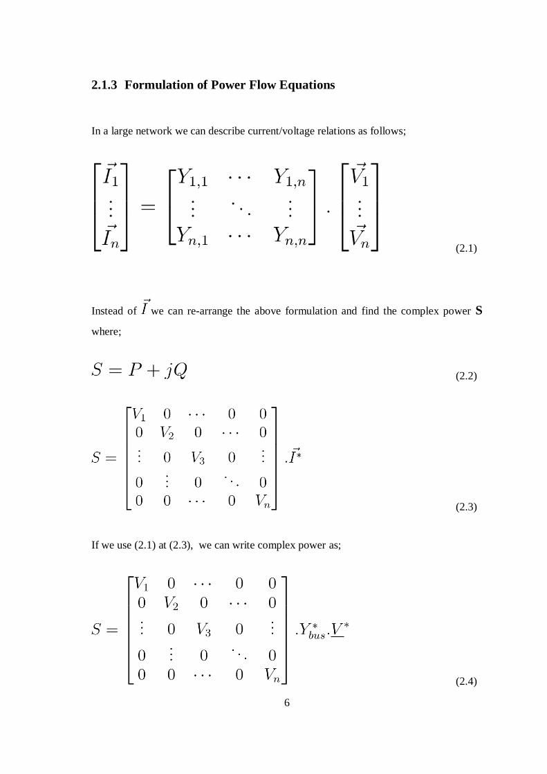
2.1.3 Formulation of Power Flow Equations

In a large network we can describe current/voltage relations as follows;

(2.1)

Instead of we can re-arrange the above formulation and find the complex power S

where;

(2.2)

(2.3)

If we use (2.1) at (2.3), we can write complex power as;

(2.4)

7

has two parts which are real and imaginary.

(2.5)

G is the real part of and known as Conductance.

B is the imaginary part of and known as Susceptance.

and also;

(2.6)

So now S can be written as;

(2.7)

which is

If we component wise this S equation;

The real part is;

(2.8)

8

(2.9)

and also the imaginary part is;

(2.10)

(2.11)

If we use KCL (Kirchhoff Current Law) for complex power balance at every bus, we

will have 2n equations. And we have 4n variables which are P,Q,V and δ for every bus.

Some of the variables are known and the others are unknown.

Bus type Number of buses Known Unknown Number of

available

equations

Slack

1 δi , |Vi| P1, Q1 0

i=1

Generator

m-1 Pi, |Vi| Δi,Qi m-1 (i=2,3,….Ng+1)

Load (Ng+2,…..N) n-m Pi, Qi Δi,Vi 2(n-m)

Total n 2n 2n 2n-m-1

Figure 2.2

9

We have m-1 P equations for generator bus and 2(n-m) P and Q equations for load bus.

So we have 2n-m-1 equations for solving n-1 δ (angles) except at bus no 1 (slack bus)

and n-m V (voltages) for load buses. To solve these 2n-m-1 unknown we use active

power balance at buses i = 2 to n and reactive power balance at bus i=m+1 to n.

We can organize 2n-m-1 unknowns and equations as vector.

(2.12)

(2.13)

Then we must find a special x* such that

2.1.4 Methods for Solution of Power Flow Analysis

There are three main methods for solving power flow. In this thesis, all three are

explained but at the program which solves the power flow analysis Newton Raphson

10

Method is used. Also, for formulation of PTDF matrix, Decoupled Load Flow Method

is taken into consideration.

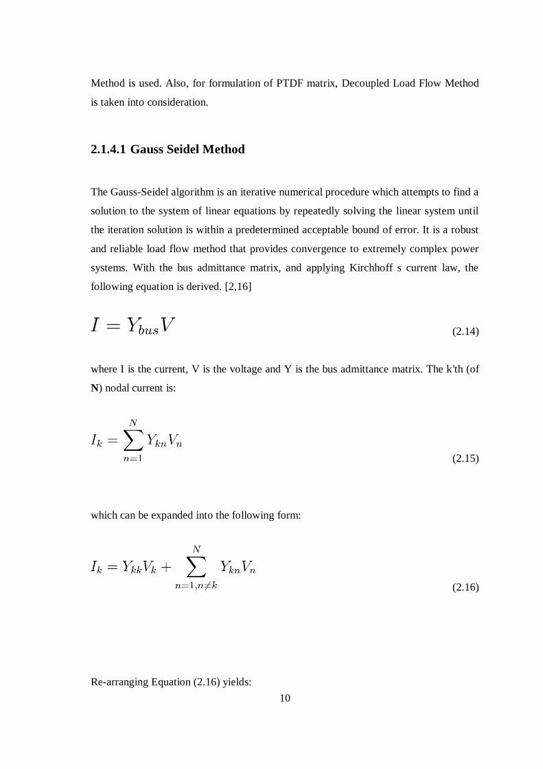
2.1.4.1 Gauss Seidel Method

The Gauss-Seidel algorithm is an iterative numerical procedure which attempts to find a

solution to the system of linear equations by repeatedly solving the linear system until

the iteration solution is within a predetermined acceptable bound of error. It is a robust

and reliable load flow method that provides convergence to extremely complex power

systems. With the bus admittance matrix, and applying Kirchhoff s current law, the

following equation is derived. [2,16]

(2.14)

where I is the current, V is the voltage and Y is the bus admittance matrix. The k'th (of

N) nodal current is:

(2.15)

which can be expanded into the following form:

(2.16)

Re-arranging Equation (2.16) yields:

11

(2.17)

Current at the k'th bus:

(2.18)

With the complex power at a given node, Equation (2.17) will yield the following result:

(2.19)

Since the Gauss-Seidel method is an iterative procedure, Equation (2.19) yields the

following:

(2.20)

From the equation (2.20), we can solve Pk and Qk, where;

(2.21)

where

12

and

(2.22)

where

2.1.4.2 Newton - Raphson (NR) Method

Newton-Raphson (NR) is iterative root finding scheme. Newton-Raphson is root finding

scheme because it is geared towards solving equations like f(x)=0. The solution to such

an equation, call it x*, is clearly a root of the function f(x) .

Starts with an initial guess which is reasonably close to the true root, then the function is

approximated by its tangent line (which can be computed using the tools of calculus),

and one computes the x-intercept of this tangent line (which is easily done with

elementary algebra). This x-intercept will typically be a better approximation to the

function's root than the original guess, and the method can be iterated.

x0=initial guess

iteration :

(2.23)

We can generalize it. Suppose we have x0 as an initial guess we use Taylor Expansion to

predict x*.

13

(2.24)

We can rearrange the equation (2.24) that:

(2.25)

Modifying this equation (2.25):

(2.26)

f and x are vectors so:

(2.27)

For the power flow problems; from the equation (2.12) the x vector is:

14

and is the Jacobean matrix J.

So Jacobean matrix J as;

(2.28)

For the initial guess (x0) we will set all δ's close to zero and all V's close to 1.0 p.u.

Consider a set of n non-linear algebraic equations

fi (x1, x2,……, xn) =0; i=1,2,3, ….., n

fi (x10 +∆x1

0, x2

0 +∆x2

0,… …….. xn

0+∆xn

0)

=0;

Taylor series expansion

fi (x10, x2

0,…..xn

0)+[(∂fi/∂x1)

0 ∆x1

0 + (∂fi/∂x2)

0 ∆x2

0+….+(∂fi/∂xn)

0

∆xn0]+ higher order terms=0

Neglecting higher order terms we can write above equation in matrix form

15

(2.29)

Or in vector matrix form;

f0+J

0∆x

0=0

J0 is known as the Jacobian matrix.

the above Equation can be written as;

f0≈ [-j

0] ∆x

0 (2.30)

Update values of x are then

x1=x

0+∆x

0 (2.31)

or, in general form of x(r+1)

th iteration

x(r+1)

=x(r)

+∆x(r)

(2.32)

Iterations are continued till equation is satisfied to any desired accuracy, i.e.;

fi(x(r)

) < ε

where ε is a specified value;

16

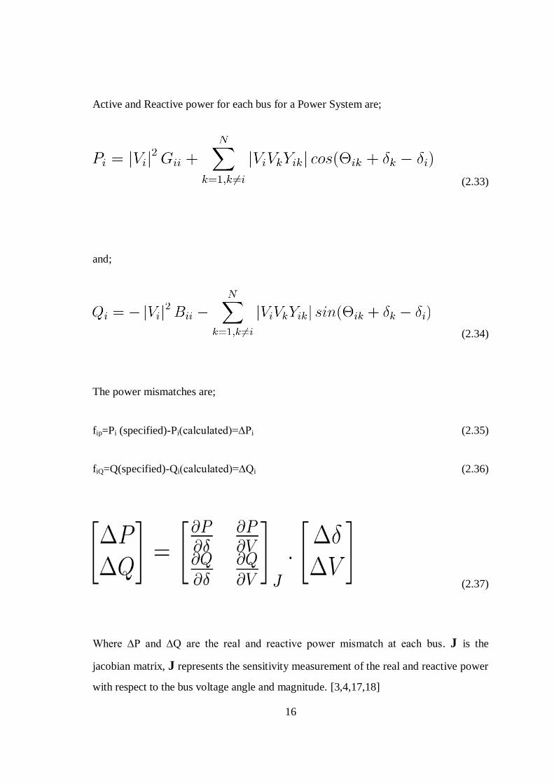
Active and Reactive power for each bus for a Power System are;

(2.33)

and;

(2.34)

The power mismatches are;

fip=Pi (specified)-Pi(calculated)=∆Pi (2.35)

fiQ=Q(specified)-Qi(calculated)=∆Qi (2.36)

(2.37)

Where ∆P and ∆Q are the real and reactive power mismatch at each bus. J is the

jacobian matrix, J represents the sensitivity measurement of the real and reactive power

with respect to the bus voltage angle and magnitude. [3,4,17,18]

17

The Newton-Raphson (NR) approach incorporating ordered elimination is the most

attractive general method it appears that many regular users of load-flow solutions are

using the NR approach.

Many advantages are attributed to the NR approach. Its convergence characteristics are

relatively powerful, compared with alternative processes, and very low computing times

are achieved when the sparse network equations are solved by the technique of sparsity-

programmed ordered elimination. [5,6,18]

Computer storage requirements are moderate and, like solution times, increase with

problem size fairly linearly, thus making the NR approach particularly attractive for

large networks. No acceleration factors have to be determined, the choice of slack bus is

rarely critical, and network modifications require negligible computing effort. The NR

formulation has great generality and flexibility, enabling a wide range of

representational requirements to be included easily and efficiently.

2.1.4.3 Decoupled Load Flow Method

The decoupled power flow method is an approximate version of Newton-Raphson

procedure [3,7]. The approximation of the Newton-Raphson procedure only affects the

iteration approach it does not reduce the accuracy of the final solution.

The principle underlying the decoupled approach is based on two observations:

Change in the voltage angle delta (δ) at a bus primarily affects

the flow of real power P in the transmission lines and leaves the

flow of reactive power Q relatively unchanged.

Change in the voltage magnitude (|V|) at a bus primarily affects

the flow of reactive power Q in the transmission lines and leaves

the flow of real power relatively unchanged.

18

We know from the formula (2.37) that the power mismatches can be written as in matrix

form as follow;

From the above equation we can assume that[8,19];

,

and

,

A well designed a properly operated power transmission system:

The angular differences (δi-δk) between typical buses of the system are usually

so small that[8];

cos(δi-δk)=1

and

sin(δi-δk)≈ (δi-δk)

The line susceptances are many times larger than the line conductance Gik so that

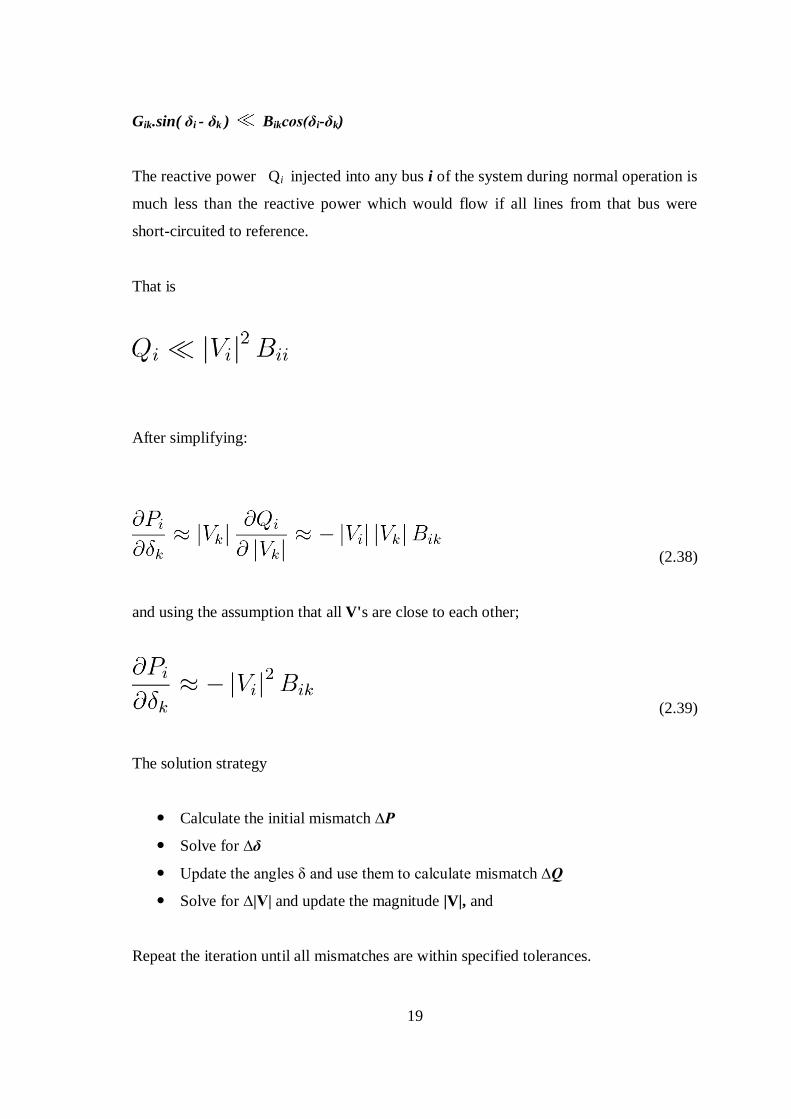
19

Gik.sin( δi - δk ) Bikcos(δi-δk)

The reactive power Qi injected into any bus i of the system during normal operation is

much less than the reactive power which would flow if all lines from that bus were

short-circuited to reference.

That is

After simplifying:

(2.38)

and using the assumption that all V's are close to each other;

(2.39)

The solution strategy

Calculate the initial mismatch ∆P

Solve for ∆δ

Update the angles δ and use them to calculate mismatch ∆Q

Solve for ∆|V| and update the magnitude |V|, and

Repeat the iteration until all mismatches are within specified tolerances.

20

2.1.5 Calculation of Power Flow of Each Line

If we consider figure 2.1. At Bus 1 we have a Voltage V1 and at bus 3 we have a

voltage V3. Between this two bus, we have Impedance Z13 or that say Admittance Y13.

Between this two buses, the current I13 flows. Actually, this I13 flows from the Bus 1. So

we can say that, the power flows from Bus 1 to Bus 3 is;

S13=V1.(I13)* (2.40)

I13=(V1-V3).Y13 (2.41)

(I13)*=[(V1-V3).Y13]* (2.42)

S13=V1.[(V1-V3).Y13]* (2.43)

and the power flows from Bus 3 to Bus 1 is;

S31=V3.[(V1-V3).Y13]* (2.44)

if we subtract S31 from S13;

S13-S31=(V1-V3)2.Y13 (2.45)

and this formula is obviously the power lost on the lines. So it means that the

formulation of line flows (2.43) is clearly true.

if we generalizes this formula;

Sjk=Vj.[(Vj-Vk).Yjk]* (2.46)

21

3 PTDF- Power Transfer Distribution Factors

3.1 Available Transfer Capability

The market is fierce in power generation and supply. Population increase and so does

the demand for electrical power. It is due to this demand that pushes us to find new

ways of not only producing more efficient power, but also to look into ways of

supplying it efficiently. This is where transfer capability steps in. Transfer capability is

an indication of how much power a power system network can supply without

compromising system security. Operators use transfer capability as judgment on the

performance of a system. If the operators know the transfer capability, and know the

present transfer values, it will be easy to find out the Available Transfer Capability.[20]

A transfer is specified by changes in power injections at buses in the network. For

example, a point to point transfer from bus A to bus B is specified by increasing power

at bus A and reducing power at bus B. In particular, if 100 MW are to be transferred

from A to B, then power at bus B is reduced by 100 MW and power at bus A is

increased by 100 MW plus an amount to cover the change in losses. In this case bus A

is called a source of power and bus B is called a sink of power.

Available Transfer Capability (ATC) is a measure of the transfer capability remaining

in the physical transmission network for further commercial activity over and above

already committed uses. Mathematically, ATC is defined as the Total Transfer

Capability (TTC) less the Transmission Reliability Margin (TRM), less the sum of

existing transmission commitments (which includes retail customer service) and the

Capacity Benefit Margin (CBM).[9,20,21]

ATC = TTC – TRM – Existing Transmission Commitments (including CBM)

22

Total Transfer Capability (TTC) is defined as the amount of electric power that can

be transferred over the interconnected transmission network in a reliable manner while

meeting all of a specific set of defined pre- and post-contingency system conditions.

Transmission Reliability Margin (TRM) is defined as that amount of transmission

transfer capability necessary to ensure that the interconnected transmission network is

secure under a reasonable range of uncertainties in system conditions.

Capacity Benefit Margin (CBM) is defined as that amount of transmission transfer

capability reserved by load serving entities to ensure access to generation from

interconnected systems to meet generation reliability requirements.[22]

Curtailability is defined as the right of a transmission provider to interrupt all or part of

a transmission service due to constraints that reduce the capability of the transmission

network to provide that transmission service. Transmission service is to be curtailed

only in cases where system reliability is threatened or emergency conditions exist.

Recallability is defined as the right of a transmission provider to interrupt all or part of

a transmission service for any reason, including economic, that is consistent with FERC

policy and the transmission provider’s transmission service tariffs or contract

provisions.

Non-recallable ATC (NATC) is defined as TTC less TRM, less non-recallable

reserved transmission service (including CBM).

Recallable ATC (RATC) is defined as TTC less TRM, less recallable transmission

service, less nonrecallable transmission service (including CBM). RATC must be

considered differently in the planning and operating horizons. In the planning horizon,

the only data available are recallable and non-recallable transmission service

reservations, whereas in the operating horizon transmission schedules are known.

23

The ATC between two areas provides an indication of the amount of additional electric

power that can be transferred from one area to another for a specific time frame for a

specific set of conditions. ATC can be a very dynamic quantity because it is a function

of variable and interdependent parameters. These parameters are highly dependent upon

the conditions of the network. Consequently, ATC calculations may need to be

periodically updated. Because of the influence of conditions throughout the network, the

accuracy of the ATC calculation is highly dependent on the completeness and accuracy

of available network data.

The system-limiting factors that limit a power system’s ATC are many. Among them

are the line current limits, voltage magnitude limit, generator reactive power limit, and

voltage collapse limit, etc.

The line current limit usually is a line’s thermal limit. Too much current flow in a line

may cause a line to droop or damage nearby connected equipments. DC power flow has

been widely used to calculate thermal limit with great speed. But DC power flow cannot

deal with other limiting factors.

The bus voltage magnitudes also need to be kept within reasonable limits. Voltage over-

limit may cause damage to system equipments, and reduce the power quality to the

customers. Low voltage sometimes is also an indication that the system is near a voltage

collapse. Both high voltage and low voltage are regulated by system circuit breakers and

pose limits to the power transfer.

Generators have reactive power output limits. After a limit is reached, a generator will

not be able to regulate its bus voltage. It is degraded from a PV bus into a PQ bus. This

may cause voltage collapse or system instability.

The voltage collapse is the upper physical limit that a power system can function

properly. Beyond this point, nonmathematical solution exists. This situation usually

happens after a bus voltage has a significant drop or when a generator’s var limit is

reached. It is not considered here since the two factors that cause it has been considered

[10,23].

24

Available Transfer Capability is important that where power system reliability meets

electricity market efficiency. ATC can have a huge impact on market outcomes and

system reliability, so the results of ATC are of great interest to all involved.

When electric power is transferred between two areas such as Area A to Area F in

Figure A1, the entire network responds to the transaction. The power flow on each

transmission path will change in proportion to the response of the path to the transfer.

Similarly, the power flow on each path will change depending on network topology,

generation dispatches, customer demand levels, other transactions through the area, and

other transactions that the path responds to which may be scheduled between other

areas.

Network conditions will vary over time, changing line loading conditions, and causing

the ATC of the network to change. Also, the most limiting facility in determining the

network’s ATC can change from one time period to another, particularly in highly

meshed networks. Therefore, the ATC of the network is time dependent.

3.2 Sensitivity

Bulk power transfers in electric power systems are limited by transmission network

security. Transfer capability measures the maximum power transfer permissible under

certain assumptions. Once a transfer capability has been computed for one set of

assumptions, it is useful to quickly estimate the effect on the transfer capability of

modifying those assumptions. Transfer capabilities must be quickly computed for

various assumptions representing possible future system conditions and then

recomputed as system conditions change. The usefulness of each computed transfer

capability is enhanced if the sensitivity of the transfer capability is also computed.[9,20]

Estimates of transfer capabilities must be updated regularly as to avoid the combined

effect of power transfers from causing an undue risk of system overloads, equipment

25

damage, or blackouts. However, being overly conservative over the estimates of transfer

capability will unnecessarily limit the power transfers and would prove to be costly and

an inefficient use of the network. If we have the sensitivity analysis of the system, the

operators can easily calculate the available transfer capacity or making scenarios for

most sensitivities line in case of the increase of a critical load.

3.3 Power Transfer Distribution Factors (PTDF) Calculations

The role of a transmission system is to transmit reliable electrical energy from

generation facilities to distribution network. At the distribution network, loads are

changes all the time. To understand the change of transmitted energy at transition

system depends of changes load, we must calculate the Power Transfer Distribution

Factors (PTDF) of the system [11,24,25].

(3.1)

(3.2)

By using Decoupled Method which mentioned in Chapter 2;

A well designed an properly operated power transmission system:

The angular differences ( δi - δk ) between typical buses of the system are

usually so small that

The line susceptances are many times larger than the line conductance Gik so that

26

So, we can consider that, and consider V's as 1 p.u.

If we rearrange the formula we can get;

(3.3)

If we take derivative of Pi with respect to δi;

(3.4)

so, we can re arrange the formula (3.4) as;

(3.5)

Taking into consideration these assumption and the simplifications, the matrix equation

for an n-bus system may be determined as ;

27

(3.6)

So, we can say that;

∆P= B . ∆δ (3.7)

Base on relation (3.7), it can be obtained:

∆δ = X . ∆P (3.8)

Where X represent the inverse of the B matrix incremented with a row and column of

zeros at the slack bus. The line and column corresponding to the slack bus of the power

system are eliminated from the matrix and the n-1 x n-1 inverse matrix is computed.

(3.9)

To finish the PTDFs calculation process, the equation of active power flow on the ik

branch is needed [11,24].

28

(3.10)

Taking into consideration the simplifications which are;

, and

but to get better result we let U's as what they are;

(3.11)

and

The elements of the susceptance matrix B are computed based on the following

relations:

The off diagonal elements:

(3.12)

When we use the (3.12) at (3.11), we can say that;

(3.13)

Now we can look deeply to the sensitivity of a line. Change on Power Flow at branch l

(from bus I to bus k) with respect to change on load at bus j:

29

(3.14)

re arrange this formula;

(3.15)

and,

(3.16)

if we use (3.8) we can say that;

we can rearrange the formula (3.16):

(3.17)

If we consider all V's as 1 p.u. than the formula is;

(3.18)

30

4 Line Security with DSM

Power systems operation becomes more important as the load demand increases all over

the world. This rapid increase in load demand forces power systems to operate near

critical limits due to economical and environmental constraints. The objective in power

systems operation is to serve energy with acceptable voltage and frequency to

consumers at minimum cost.

Since generation and transmission units have to be operated at critical limits voltage

stability problems may occur in power system when there is an increase in load demand.

Voltage instability is one of the main problems in power systems. In voltage stability

problem some or all buses voltages decrease due to insufficient power delivered to

loads.

4.1 Definition of Voltage Stability

Voltage stability is the ability of a power system to maintain steady acceptable voltages

at all buses in the system under normal operating conditions and after being subjected to

a disturbance [12,26,27].

Loads are the main driving force of voltage instability, and that is why the voltage

instability is also called as load instability. Exact modeling of load is a difficult task

because the system loads are aggregation of many different devices. The heart of the

problem is the identification of system load composition at a given time and aggregation

of various loads. When a severe disturbance, such as fault, line tripping, etc., occurs, the

voltage of some buses reduces drastically. Reduction of system voltage may cause to

stall the heavily loaded induction motors and that may ultimately lead to voltage

instability [13,26,27].

31

It is clear that load is one of the important variables in a power system.

Controlling the load is important, but first we must know which loads are more

important and most effective for a transmission system. To understand this, sensitivity

analysis and demand side management can help us.

4.2 Sensitivity and Demand Side Management

Voltage stability can be attained by sufficient generation and transmission of energy. If

the loads increase and assume that we have sufficient generation, the transmission

system transfer capacity (transmission of energy) is the most important factor for keep

the system alive. Increase of a load, effects all lines differently. Sensitivity analysis of a

transmission system gives us this information. After this analysis, we can calculate the

flow of lines after the increase of a certain load.

By using sensitivity, after increase of loads, we can see that some of line flows exceed

their limits. This means that, increase of these loads make system collapse. By using

Demand Side Management, we could have opportunity to reduce these loads and make

the system secure.

Maximum customer benefit derives from minimum cost and sufficient supply

availability. At times, lower cost implies risk of potential unavailability of enough

power. Customers willing to share in “availability risk” can derive further benefit by

way of participating in controlled outage programs. Specifically whenever utilities

foresee dangerous loading patterns, there is a need for a rapid reduction in demand

either system-wide or at specific locations. The utility needs to get some relief in order

to solve its problems quickly and more efficiently without wasting energy. This relief

can come from customers who agree to curtail their loads upon request in exchange for

an incentive fee [14,28,29].

If we have sensitivities of all loads to all lines, it will be easier to calculate or estimate

the cost of reduction of a load. If a load is most effective of a certain line which is in

trouble (going to exceeds the limits of power transfer capability), we can say that this

32

load is most valuable for that line and worth to pay more for curtailing. If the utility has

these information, it can be easily offer a contract to a customer whose load is valuable.

Without these information, utility may pay more for less valuable loads.

4.3 Sensitivity of Line Flows to Individual Loads

The sensitivity of a line flow to each load in the system (ΔPkm/ΔPi, where ΔPkm is the

flow on the line from bus k to bus m and ΔPi is the change in load at bus i) can be

computed to help the utility relieve line overloads. When a transmission line gets

overloaded it is important to know which load has the most impact on this line

flow.[15,29]

Numerically, the sensitivity of a line flow to an individual load, can be practically

calculated as;

1- Calculate the power flow of the line Pkm-first for a stable system.

2- Change the individual load and write ΔPi as Pi-first - Pi-last

3- Re-calculate the power flow of line Pkm-last by using Pi-last

4- Calculate the change of power flow of the line as; ΔPkm= Pkm-first - Pkm-last

5- Calculate the sensitivity of the line flow to the load as; ΔPkm/ΔPi

At Power Transfer Distribution Factors (PTDF) Calculations, we create a formulation

for calculating this sensitivities. When we will look deeply to the results we can see that

there are some differences between the numerical sensitivities and the calculated

(PTDF) sensitivities.

4.4 Congestion Management

Congestion is a situation where the demand for transmission capacity exceeds the

transmission network capabilities, which might lead to a violation of network security

limits, being thermal, voltage stability limits or a (N-1) contingency condition.

33

Therefore, in a physical sense congestion is merely an indication of a presence of

transmission constraints.

One way to handle transmission contingency is load shading. But the important point is

which load is the most effective for the mentioned transmission line. To know this, we

can use sensitivity analysis for the power system. When we know the sensitivity of a

line flow to a load, this means that, we know the rate of current decrease after curtailing

a load.

Where is the change of power flow on transmission line x, and

is the change of power of load at bus no n.

34

5 Simulation and Results

The power flow analysis method presented in Chapter 2 is applied to a 6-bus sample test

system and then we calculate the sensitivities of all lines to all loads. For simulating and

testing the system, there are some professional tools. Instead of using those tools, at this

thesis, I preferred to write a program. This made the system and theoretical calculation

more understandable.

This program has ability to compute power flow analysis, the flows on each line and the

sensitivities of all line flows with respect to all loads of a system which has IEEE

common format file. The number of lines, generators, loads or buses do not affect the

running of the program. It can handle a power system with even thousands of buses

which has a properly prepared common format file.

5.1 Six Bus Sample Test System

Sample test system consists of 6 buses, 3 generators, 11 transmission lines and 3 loads.

The single line diagram of 6-bus test system is shown in Figure (fig 5.1). The IEEE

common format data of this system can be seen below.

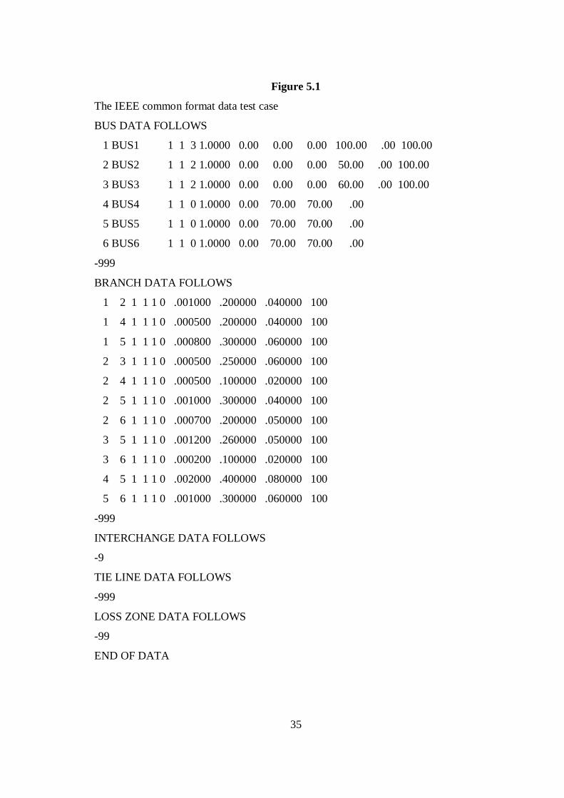
35

Figure 5.1

The IEEE common format data test case

BUS DATA FOLLOWS

1 BUS1 1 1 3 1.0000 0.00 0.00 0.00 100.00 .00 100.00

2 BUS2 1 1 2 1.0000 0.00 0.00 0.00 50.00 .00 100.00

3 BUS3 1 1 2 1.0000 0.00 0.00 0.00 60.00 .00 100.00

4 BUS4 1 1 0 1.0000 0.00 70.00 70.00 .00

5 BUS5 1 1 0 1.0000 0.00 70.00 70.00 .00

6 BUS6 1 1 0 1.0000 0.00 70.00 70.00 .00

-999

BRANCH DATA FOLLOWS

1 2 1 1 1 0 .001000 .200000 .040000 100

1 4 1 1 1 0 .000500 .200000 .040000 100

1 5 1 1 1 0 .000800 .300000 .060000 100

2 3 1 1 1 0 .000500 .250000 .060000 100

2 4 1 1 1 0 .000500 .100000 .020000 100

2 5 1 1 1 0 .001000 .300000 .040000 100

2 6 1 1 1 0 .000700 .200000 .050000 100

3 5 1 1 1 0 .001200 .260000 .050000 100

3 6 1 1 1 0 .000200 .100000 .020000 100

4 5 1 1 1 0 .002000 .400000 .080000 100

5 6 1 1 1 0 .001000 .300000 .060000 100

-999

INTERCHANGE DATA FOLLOWS

-9

TIE LINE DATA FOLLOWS

-999

LOSS ZONE DATA FOLLOWS

-99

END OF DATA

36

5.2 Simulation Program

The simulation program was written in MATLAB.

It contains several phases which are;

a. Reading the common format file:

Program has the ability to read any common format file which is prepared for any High

Voltage System. The size of the system does not cause a problem for the program.

b. Formation of Y-Bus of the system:

This part of the program forms the Y-Bus matrix of the system by directly reading bus

and branch information from common format file.

c. Calculation of Active and Reactive power for each Bus.

At this part of the program, Active and Reactive Power mismatches are calculated by

using the Newton Raphson Method.

d. Controlling the tolerance for ending the iterations

This part of the program checks the tolerance and when it is small enough stops the

iteration. This is important because the tolerance has to be small enough for better

results and big enough for ending iteration in a short time. And for a big power system,

sometimes seconds are too big to make a decision.

e. Calculation of power flow each line

At this part of the program, all line flows are calculated. This formula is derived in

section 2.1.5. (formula (2.26)).

37

f. Sensitivity Calculations:

Here, the sensitivity of all loads to all line flows are calculated. Two separate

formulations are used here. The first one comes from the formula 3.18 and the second

one comes from the formula 3.17. Two separate but very close results can be seen from

these formulas.

g. Compare the results by using Matpower4 and numerical

sensitivities.

This part of the program shows all sensitivity results and makes comparisons.

Sensitivities come from the professional tool Matpower4, sensitivities from the

numerical applications and two other sensitivities are calculated at the "sensitivity

calculation" of the program. All differences and all differences in percentages between

sensitivities can be calculated at this part.

38

5.3 Results

Program results have a lot of information for the power system;

From the results we can see the Y-Bus of the system. For 6-bus sample test system the

result of Y-Bus calculated as 6x6 (nxn) matrix:

After that, Voltages, Angles, Active Power and Reactive power for all bus, which is 6

for this test system, can be calculated as a 6x1 matrix.

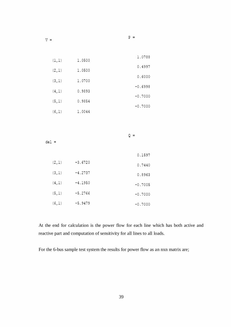
39

At the end for calculation is the power flow for each line which has both active and

reactive part and computation of sensitivity for all lines to all loads.

For the 6-bus sample test system the results for power flow as an nxn matrix are;

40

The elements of nxn matrix, for example Pij, shows the flow of power from bus i to bus

j.

When we look the results for sensitivity, we can see lxn matrix, which l is the number of

transmission lines and n is the number of buses. The elements show us the sensitivity of

line l with respect to load buses at n.

41

If we consider all V's as 1 p.u. then the results change a little;

Rather than the calculated sensitivities, we have also numerical application sensitivities

which are mentioned in section 4.3. This was obtained by changing the loads one by one

and looking at the power flow changes at each line.

42

After calculations, we have one more phase which is the comparison of the results with

a professional tool called Matpower4. The program both shows the sensitivity (PTDF)

matrix computed by Matpower4 and the difference between matrixes computed by my

program.

Now we have 4 different sensitivity matrixes. If we calculate the differences between

Sensitivity Matrix which is calculated from the formula (3.17), and Numerical

Sensitivity, and differences between Sensitivity Matrix which is calculated from the

formula (3.18), and Numerical Sensitivity, we can see that using V's as what they are

improve the results. Differences:

43

1- The differences in percentage between sensitivity matrix which use the

formula (3.17) and Numerical sensitivity matrix is;

perTDifV = % 3.7286

2- The differences in percentage between sensitivity matrix which use the

formula (3.18) and Numerical sensitivity matrix is;

perTDif = % 5.5087

3- The differences in percentage between sensitivity matrix which calculated by

using Matpower and Numerical sensitivity matrix is;

perTDifH = % 2.8438

44

5.4 Results for 14 Bus System and Analysis of these Results

To understand deeply the Sensitivity Analysis and what will happen after changing of

load a14 Bus System is used. For the 14 Bus system, by using the simulation program,

all power flow calculations for each bus and load flows for branches and PTDF matrix

are calculated. After that, load at bus 6 is doubled. First it was 11.2 MW. After all

calculations, I changed the load at bus 6 as 22.4 MW and make all calculations by using

the program.

This 14 Bus test system consists of 14 buses, 2 generators, 3 Synchronous Condensers

which are regard as generator bus and 9 loads. Also this system has 20 transmission

lines. The single line diagram of 14-bus test system is shown in Figure (fig 5.2).

Figure 5.2

45

When we execute the program we can get the following results for each bus as a nodal

value.

Bus Bus Type Voltage Generation Load

No Mag(pu) Ang(rad) P(MW) Q(MVAr) P(MW) Q(MVAr)

1 slack 1,0600 0,00 232,39 -16,55 0,00 0,00

2 Generator 1,0450 -0,09 40,00 43,56 21,70 12,70

3 Generator 1,0100 -0,22 0,00 25,08 94,20 19,00

4 Load 1,0177 -0,18 47,80 -3,90

5 Load 1,0195 -0,15 7,60 1,60

6 Generator 1,0700 -0,25 0,00 12,73 11,20 7,50

7 Load 1,0615 -0,23 0,00 0,00

8 Generator 1,0900 -0,23 0,00 17,62 0,00 0,00

9 Load 1,0559 -0,26 29,50 16,60

10 Load 1,0510 -0,26 9,00 5,80

11 Load 1,0569 -0,26 3,50 1,80

12 Load 1,0552 -0,26 6,10 1,60

13 Load 1,0504 -0,26 13,50 5,80

14 Load 1,0355 -0,28 14,90 5,00

Table 5.1

Here at table 5.1, we can see all power generation and all loads of each bus. As

mentioned at section 3.3, we need line flows to understand the sensitivities. As the

sensitivity of a line with respect to any load is the power flow difference at this branch

divided by the load change at the load bus.

After execution of the program, we can get all power flows for each branch as follows;

Branch From To From Bus Injection To Bus Injection

No Bus Bus P(MW) Q(MVAr) P(MW) Q(MVAr)

1 1 2 156,88 -20,40 -152,59 27,68

2 1 5 75,51 3,85 -72,75 2,23

46

3 2 3 73,24 3,56 -70,91 1,60

4 2 4 56,13 -1,55 -54,45 3,02

5 2 5 41,52 1,17 -40,61 -2,10

6 3 4 -23,29 4,47 23,66 -4,84

7 4 5 -61,16 15,82 61,67 -14,20

8 4 7 28,07 -9,68 -28,07 11,38

9 4 9 16,08 -0,43 -16,08 1,73

10 5 6 44,09 12,47 -44,09 -8,05

11 6 11 7,35 3,56 -7,30 -3,44

12 6 12 7,79 2,50 -7,71 -2,35

13 6 13 17,75 7,22 -17,54 -6,80

14 7 8 0,00 -17,16 0,00 17,62

15 7 9 28,07 5,78 -28,07 -4,98

16 9 10 5,23 4,22 -5,21 -4,18

17 9 14 9,43 3,61 -9,31 -3,36

18 10 11 -3,79 -1,62 3,80 1,64

19 12 13 1,61 0,75 -1,61 -0,75

20 13 14 5,64 1,75 -5,59 -1,64

Table 5.2

Here at Table 5.2, we can see all power flow for every branch as both way. We can see

both from bus injection and to bus injection. So it is now easy to calculate all losses at

every branch. If we look the differences between power flow for from injection and to

injections, this gives us the losses.

At Table 5.3, we can see all losses for each branch and also the total loss of power at the

system. When we calculate all active powers at all bus at Table 5.1, we can see that it is

259 MW. So the total load of the system is 259 MW but the total generation is 272.39

MW. This means that, the total losses of the system also produce and this is generated

by Slack Bus. So this is the proof of the explanation of the Slack Bus that pick up the

losses of the system.

47

Branch From To Power Loss at Each Branch No Bus Bus

P(MW) Q(MVAr)

1 1 2 4,30 7,27

2 1 5 2,76 6,08

3 2 3 2,32 5,16

4 2 4 1,68 1,47

5 2 5 0,90 0,93

6 3 4 0,37 0,36

7 4 5 0,51 1,62

8 4 7 0,00 1,70

9 4 9 0,00 1,30

10 5 6 0,00 4,42

11 6 11 0,06 0,12

12 6 12 0,07 0,15

13 6 13 0,21 0,42

14 7 8 0,00 0,46

15 7 9 0,00 0,80

16 9 10 0,01 0,03

17 9 14 0,12 0,25

18 10 11 0,01 0,03

19 12 13 0,01 0,01

20 13 14 0,05 0,11

TOTAL 13,39 32,70

Table 5.3

The last important result after this power flows is the Power Transfer Distribution

Factors matrix. The elements of this matrix are the Sensitivities of line flows with

respect to Loads. In any Power System, if we have l branches and n buses, this means

that the Sensitivity matrix dimensions are l x n.

48

Table 5.4

49

Here at table 5.4, let say at colon 6, we have 20 different numbers. These numbers give

us the sensitivities of each line (branch) with respect to load at bus no 6. The fist

number of this colon is 0.6291. The meaning of this number is that, if we reduce this

load by 1 MW the power flow at branch 1 (The line from bus 1 to bus 2) reduces by

0,6291 MW. All numbers at this colon have the similar meaning. Second number gives

us the ratio of change power flow at branch 2 with respect to change of load at bus 6.

So, the lth number at colon 6 gives us the ratio of power flow change at branch l with

respect to change of load at bus 6. Now we are able to calculate the new active power

flow for each branch after this load at bus 6 change.

Suppose the load at bus 6 increases by 11.2 MW and reach 22.4 MW. Again we can

assume that the load change at bus 6 as 11.2 MW. Also we know the previous active

power flow for every bus. If we multiply these previous active power flows with this

change of load and with the sensitivity of each line with respect to load change at bus 6,

we will find the new active power flows for every branch.

Branch No

From Bus To Bus

Previous Active Power Flow

PTDF of each Line Flows wrt Load 6

Active Power Flow after Load 6 increase by

11.2 MW

P(MW) P(MW)

1 1 2 156,88 -0,6291 163,93

2 1 5 75,51 -0,3709 79,66

3 2 3 73,24 -0,1188 74,57

4 2 4 56,13 -0,2487 58,92

5 2 5 41,52 -0,2616 44,45

6 3 4 -23,29 -0,1188 -21,95

7 4 5 -61,16 -0,0389 -60,72

8 4 7 28,07 -0,2075 30,40

9 4 9 16,08 -0,1211 17,44

10 5 6 44,09 -0,6714 51,61

11 6 11 7,35 0,1979 5,14

12 6 12 7,79 0,0291 7,46

13 6 13 17,75 0,1017 16,61

14 7 8 0,00 0,0000 0,00

15 7 9 28,07 -0,2075 30,40

50

16 9 10 5,23 -0,1979 7,44

17 9 14 9,43 -0,1307 10,89

18 10 11 -3,79 -0,1979 -1,57

19 12 13 1,61 0,0291 1,29

20 13 14 5,64 0,1307 4,18

Table 5.5

Table 5.5 shows us the new calculated active power flow of each branch after the load

at bus 6 increase by 11.2 MW. These values are calculated by using the sensitivities of

all lines with respect to load 6. At the section 4.3, the method for calculation of

numerical sensitivity explained. To see and prove this, at this 14 bus test system, load at

bus 6 increased by 11.2 MW and the simulation program execute again. After this

execution, we get new results for the system.

Bus Bus Type Voltage Generation Load

No Mag(pu) Ang(rad) P(MW) Q(MVAr) P(MW) Q(MVAr)

1 slack 1,0600 0,00 244,71 -17,84 0,00 0,00

2 Generator 1,0450 -0,09 40,00 47,13 21,70 12,70

3 Generator 1,0100 -0,23 0,00 25,88 94,20 19,00

4 Load 1,0162 -0,19 47,80 -3,90

5 Load 1,0176 -0,16 7,60 1,60

6 Generator 1,0700 -0,27 0,00 15,67 22,40 7,50

7 Load 1,0614 -0,25 0,00 0,00

8 Generator 1,0900 -0,25 0,00 17,72 0,00 0,00

9 Load 1,0566 -0,28 29,50 16,60

10 Load 1,0516 -0,28 9,00 5,80

11 Load 1,0574 -0,28 3,50 1,80

12 Load 1,0551 -0,29 6,10 1,60

13 Load 1,0506 -0,29 13,50 5,80

14 Load 1,0360 -0,30 14,90 5,00

Table 5.6

We can see from Table 5.6 that the load at bus 6 is change. This load changing, change

all system calculated data (or measured data in a Power System). The generation at

51

slack bus change. Some of the voltages and angle at the buses also change. So it is

obvious that Power Flows are going to change. Now we can calculate these new power

flows for every branch.

Branch From To From Bus Injection To Bus Injection

No Bus Bus P(MW) Q(MVAr) P(MW) Q(MVAr)

1 1 2 164,71 -22,21 -159,97 30,85

2 1 5 80,00 4,38 -76,90 3,12

3 2 3 74,69 3,42 -72,28 2,13

4 2 4 59,02 -1,36 -57,17 3,37

5 2 5 44,55 1,52 -43,51 -2,02

6 3 4 -21,92 4,75 22,26 -5,21

7 4 5 -60,51 16,67 61,02 -15,07

8 4 7 30,28 -10,21 -30,28 12,19

9 4 9 17,34 -0,73 -17,34 2,25

10 5 6 51,79 12,37 -51,79 -6,38

11 6 11 5,21 4,32 -5,17 -4,24

12 6 12 7,53 2,64 -7,46 -2,50

13 6 13 16,65 7,58 -16,46 -7,20

14 7 8 0,00 -17,25 0,00 17,72

15 7 9 30,28 5,07 -30,28 -4,15

16 9 10 7,35 3,43 -7,34 -3,38

17 9 14 10,77 3,08 -10,62 -2,78

18 10 11 -1,66 -2,42 1,67 2,44

19 12 13 1,36 0,90 -1,35 -0,90

20 13 14 4,31 2,30 -4,28 -2,22

Table 5.7

Table 5.7 shows the new calculated power flows for each branch by using the data

calculated from Newton Rapson Method at Table 5.6.

The differences between 2 methods which can be used for calculating new power flows

after changing a load is:

52

a- To find the new power flows at Table 5.5 we don’t solve all the system

again after changes. We use PTDF and old data and calculate simply the new values for

each branch.

b- To find the new power flows at Table 5.7 we directly calculate

everything for the system at the beginning which explained at chapter 2 and find all

power flows for every branch.

Now, for the next step, we can use these two different power flows and the two different

load value at bus 6 and can calculate PTDF for all branch with respect to load 6.

Branch From To

From Bus Injection

before Load 6 change

From Bus Injection after

Load 6 change

PTDF of any branch wrt

Load 6

No Bus Bus P(MW) P(MW) ΔPl /ΔP6

1 1 2 156,88 164,71 -0,6987

2 1 5 75,51 80,00 -0,4010

3 2 3 73,24 74,69 -0,1299

4 2 4 56,13 59,02 -0,2579

5 2 5 41,52 44,55 -0,2711

6 3 4 -23,29 -21,92 -0,1217

7 4 5 -61,16 -60,51 -0,0576

8 4 7 28,07 30,28 -0,1969

9 4 9 16,08 17,34 -0,1127

10 5 6 44,09 51,79 -0,6876

11 6 11 7,35 5,21 0,1915

12 6 12 7,79 7,53 0,0231

13 6 13 17,75 16,65 0,0978

14 7 8 0,00 0,00 0,0000

15 7 9 28,07 30,28 -0,1969

16 9 10 5,23 7,35 -0,1899

17 9 14 9,43 10,77 -0,1197

18 10 11 -3,79 -1,66 -0,1894

19 12 13 1,61 1,36 0,0228

20 13 14 5,64 4,31 0,1188

Table 5.8

53

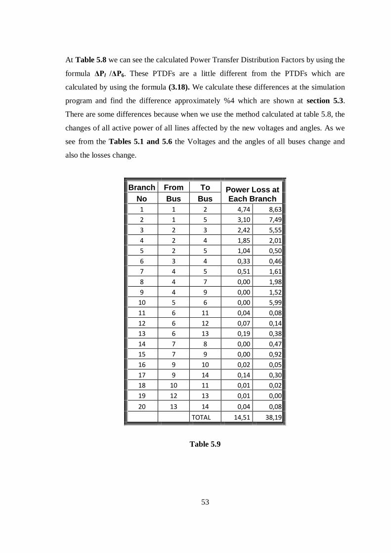
At Table 5.8 we can see the calculated Power Transfer Distribution Factors by using the

formula ΔPl /ΔP6. These PTDFs are a little different from the PTDFs which are

calculated by using the formula (3.18). We calculate these differences at the simulation

program and find the difference approximately %4 which are shown at section 5.3.

There are some differences because when we use the method calculated at table 5.8, the

changes of all active power of all lines affected by the new voltages and angles. As we

see from the Tables 5.1 and 5.6 the Voltages and the angles of all buses change and

also the losses change.

Branch From To Power Loss at Each Branch No Bus Bus

1 1 2 4,74 8,63

2 1 5 3,10 7,49

3 2 3 2,42 5,55

4 2 4 1,85 2,01

5 2 5 1,04 0,50

6 3 4 0,33 0,46

7 4 5 0,51 1,61

8 4 7 0,00 1,98

9 4 9 0,00 1,52

10 5 6 0,00 5,99

11 6 11 0,04 0,08

12 6 12 0,07 0,14

13 6 13 0,19 0,38

14 7 8 0,00 0,47

15 7 9 0,00 0,92

16 9 10 0,02 0,05

17 9 14 0,14 0,30

18 10 11 0,01 0,02

19 12 13 0,01 0,00

20 13 14 0,04 0,08

TOTAL 14,51 38,19

Table 5.9

54

At Table 5.9 we can see that the losses increase. For the Active Power, the losses

increase as 1,12 MW. This is why the Active Power at Table 5.5 and 5.7 are different.

The calculation method which is used for the Table 5.5 ignores the changes of losses.

At chapter 4, Demand Side Management by using Sensitivity Analysis is explained. If

we look closer to Table 5.4, which has the data of PTDF, we can understand how this

PTDF values can help any Utility to make contracts with customers and manage the

Loads. Here the first element of the colon 2 is 0.838. This means that for branch no. 1,

which is from bus 1 to bus 2, Load at bus 2 is the most valuable. Now for preventing

congestion at branch 1, it is worth to pay more for curtailing this load at bus 2. Again if

we look the value at colon 2 row 16, it is 0,0028. If we have congestion at branch no 16,

it will not be worth to pay for curtailing the Load at bus 2. All values at this Table 5.4

help the utility about these contracts.

55

6 Conclusion

It is clear that the most effective method for calculation of PTDF matrix is the physical

parameters of the lines of the network. But, if we try to use all physical parameters, it is

almost impossible to solve it mathematically. The best way is making assumptions by

using well known approximation methods and matrix manipulation techniques.

Using these PTDF matrices can help the system operator for making better plans. But

every system and electricity market has its own dynamics and when we talk about load

curtailing, we must consider some other things like ATC (Available Transfer Capacity).

Sometimes, the most effective line for an individual load may have a large ATC and

there is no meaning curtailing that load to relieve the network. But if we take into

consideration sensitivity of all loads to all lines and if we have a line which is

congested, now we can say that which load can be curtailed to help us relieve that line.

56

REFERENCES

[1] I J Nagrath, D.P. Kothari, "Modern Power System Analysis", Tata McGraw Hill

Publishing Limited. ISBN 0-07-049489-4

[2] G.M Gilbert, D.E.Bouchard, and A.Y. Chikhani, "A Comparison Of Load Flow

Analysis Using Distflow, Gauss-Seidel, And Optimal Load Flow Algorithms"

Department of Electrical and Computer Engineering Royal Military College of

Canada Kingston, Ontario, K7K 5LO. 0-7803-43 14-X/98/$10.0001998 IEEE

[3] B. Stott, "Effective Starting Process for Newton-Raphson Load Flows."

M.Sc.Tech. PROC. IEE, Vol. 118, No. 8, August 1971

[4] Vander Menengoy da Costa, Nelson Martins, Josk Luiz R. Pereira,

"Developments in the Newton Raphson Power Flow Formulation Based on

Current Injections." IEEE Transactions on Power Systems, Vol. 14, No. 4,

November 1999

[5] Tinney, w. F., and Hart, c. E., "Power Flow Solution By Newton's Method."

IEEE Trans., 1967, PAS-86, pp. 1449-1456

[6] Tinney, W. F., And Walker, J. w.:, "Direct Solutions Of Sparse Network

Equations By Optimally Ordered Triangular Factorisation." Proceedings of the

IEEE Vol:55, No:11, 1967

[7] Stott, B.; "Decoupled Newton Load Flow." Power Apparatus and Systems, IEEE

Transactions on Volume: PAS-91 , Issue: 5, Publication Year: 1972 , Page(s):

1955 - 1959 IEEE Journals

[8] B. Stott 0. Alsaç. "Fast Decoupled Load Flow." IEEE PES Summer Meeting &

EHV/UHV Conference, Vancouver, B.C. Canada, July 15-20, 1973

[9] Scott Greene, Ian Dobson, Fernando L. Alvarado. "Sensitivity of Transfer

Capability Margins With a Fast Formula." IEEE TRANSACTIONS On Power

Systems, VOL. 17, NO. 1, February 2002

[10] Ronghai Wang, Robert H. Lasseter, Jiangping Meng, Fernando L. Alvarado.

"Fast Determination of Simultaneous Available Transfer Capability (ATC)."

ECE Dept. University of Wisconsin-Madison 1415 Engineering Drive Madison,

WI 53706

57

[11] Barbulescu,C.; Kilyeni,S.; Vuc,G.; Lustrea,B.; Precup,R.-E.; Preid,S. "Software

Tool For Power Transfer Distribution Factors (PTDF) Computing Within The

Power Systems." EUROCON '09. IEEE. Issue Date : 18-23. May2009 On

page(s): 517

[12] P. Kundur, "Power System Stability and Control." McGraw-Hill, 1994.

[13] M.H.Haque and U.M.R.Pothula. "Evaluation of Dynamic Voltage Stability of a

Power System." PowerCon 2004. Issue Date: 21-24 Nov. 2004. Volume: 2. On

page(s): 1139

[14] Murat Fahrioğlu, Fernando L. Alvarado. "The Design Of Optimal Demand

Management Programs." Department of Electrical and Computer Engineering,

The University of Wisconsin – Madison

[15] M. Fahrioğlu, "The Design of Optimal Electric Power Demand Management

Contracts." Phd. Thesis. Superviser Professor Fernando Alvarado, University of

Wisconsin-Madison.

[16] Turan Gonen, "Elecaic Power Distribution System Engineering", McGraw-Hill

Publishing Company, Toronto, 1986.

[17] Dommel, H. w., Tinney, w. F., and Powell, w. L. : 'Further developments in

Newton's method for power-system applications'. IEEE winter power meeting,

New York, 1970, Paper 70 CP 161 -PWR

[18] B. Stott. "Review of load-flow calculation methods." Proceedings of IEEE,

62:916-929, July 1974.

[19] S.T.Despotovic, B.S.Babic and V.P.Mastilovic, "A rapid and reliable method for

solving load flow problems", IEEE Trans. (Power Apparatus and Systems),Vol.

PAS-90, pp. 123-130, January/February 1971.

[20] "Available Transfer Capability Definition and Determination", North American

Electric Reliability Council, June 1996.

[21] G.C. Ejebe, J. Tong, J.G. Waight, J.G. Frame, X. Wang, and W.F. Tinney,

“Available transfer capability calculations", IEEE Trans Power Syst., vo1.13, pp.

1521-1527, Nov. 1998.

[22] Sauer, P.W.; " Technical Challenges of Computing Available Transfer

Capability (ATC) in Electric Power Systems" System Sciences, 1997,

Proceedings of the Thirtieth Hawaii International Conference on Vol. 5,Digital

58

Object Identifier: 10.1109/HICSS.1997.663220 ,1997 , Page(s): 589 - 593, IEEE

Conferences

[23] F.L. Alvarado and T.H. Jung, “Direct detection of voltage collapse conditions,”

Proceedings: Bulk power system voltage phenomena – Voltage stability and

security, EPRI-6183, pp523-538, Jan. 1989.

[24] P. W. Sauer, “On the formulation of power distribution factors for linear load

flow methods,” IEEE Transactions on Power Apparatus and Systems, vol.100,

no. 2, pp. 764–770, February 1981.

[25] Asihwani Kumar, S.C. Srivastava," AC Power Transfer Distribution Factors for

Allocating Power Transactions in a Deregulated Market" IEEE, Vol.22, Issue.7,

2002

[26] Wiszniewski, A., " New Criteria of Voltage Stability Margin for the Purpose of

Load Shedding", IEEE Transactions on Volume: 22 , Issue: 3, 2007

[27] C. W. Taylor, “Power System Voltage Stability,” New York McGraw Hill,

1994.

[28] Michael Beenstock. "Generators and the cost of electricity outages." Energy

Economics, 1991.

[29] D. W. Caves, J. A. Herriges, and R. J.Windle. "The cost of electric power

interruptions in the industrial sector." Land Economics, 68(1):49–61, 1992.