ncorrmanual_v1_2

Ncorr

Instruction Manual Version 1.2

6/7/2014

Justin Blaber ([email protected])

Antonia Antoniou ([email protected]) Georgia Institute of Technology

Table of Contents

1 - Installation

1.1 - Installation Requirements

1.2 - MEX Setup

1.3 - Automatic Installation

1.4 - Manual Installation

2 - User Guide – General DIC

2.1 - Program Flow

2.2 - Setting the Reference Image

2.3 - Setting the Current Image

2.4 - Setting the Region of Interest

2.5 - Setting DIC Parameters

2.6 - DIC Analysis

2.7 - Formatting Displacements

2.8 - Strain Analysis

2.9 - Plotting

2.10 - Directly Obtaining and Altering the DIC Data

3 - User Guide – High Strain

3.1 - High Strain DIC Analysis

4 - User Guide – Discontinuous Displacements

4.1 - Discontinuous Displacements DIC Analysis

Installation Requirements - 1.1

1.1 - Installation Requirements

Version Requirements:

Required: R2009a+

Recommended: R2012a+

NOTE: Ncorr was developed on MATLAB R2009a and has not been tested on prior versions. It works best on MATLAB R2012a

and above, as R2009a has some problems with the stacking order of objects in the plotting tool.

Toolboxes Requirements:

Required: Image Processing Toolbox

Required: Statistics Toolbox

Operating System Requirements:

Required: Windows or Linux

Recommended: Windows

NOTE: Ncorr was developed on Windows 7. It has also been tested on Linux Ubuntu 11.10. Ncorr currently will not work on mac

OS.

MEX Compiler Requirements:

Recommended: Visual Studio 2005 (8.0) + or GCC 4.2+

NOTE: Ncorr has an option to use OpenMP for users with multicore processors. OpenMP requires the compilers listed above; if

the use of OpenMP is omitted, then any C++ compiler that supports the STL library should work.

MEX Setup - 1.2

1.2 - MEX Setup

First, make sure MEX has been set up properly in MATLAB. Type "mex -v" in the MATLAB terminal as

shown below:

The output will either be:

or:

In the first case, MEX has not been set up so, so choose Microsoft Visual C++ (or GCC on Linux systems)

and install it. In the second case, MEX has already been set up, but check to make sure the correct

compiler is installed. If "COMPILER = cl" or "COMPILER = gcc," then MEX is set up with the correct

compiler. If a different compiler is installed, rerun the MEX setup by typing "mex -setup" in the MATLAB

terminal as shown below:

And select either Microsoft Visual C++ (or GCC on Linux systems) from the list that appears.

Automatic Installation - 1.3

1.3 - Automatic Installation

After MEX is set up correctly, get the latest version of Ncorr from the ncorr.com website downloads

section (as of this manual, the latest version is 1.2), as shown below:

Then, navigate to the directory where you saved Ncorr. Make sure none of the files have been moved or

altered. From there, type "handles_ncorr = ncorr" in the MATLAB terminal as shown below:

A dialogue box will appear about OpenMP support. Click the checkbox for OpenMP if you have a

multicore processor and want multicore support. The number of cores on your system is most easily

determined by checking the task manager on Windows (or system processes on Linux) as shown below:


In my case, my computer has 8 logical cores that can be utilized for computation.

NOTE: If you use all your cores during computation, generally any other applications on the computer will slow down drastically

(such as browsing the internet), so if you plan on using your computer during computation, then it might be best to leave out a

core or two.

The manual compiler specification option is there for the case that GCC is installed on Windows through

gnumex. This is probably won't be the case for most users, so when in doubt leave it unchecked.

During installation, a pop-up for setting the path will appear. The path needs to be set in order to upload

images from other directories. This is only a temporary solution and the dialogue box will reappear if

MATLAB is closed and reopened. For a more permanent solution, you can set the path manually

through: File > Set Path > Add Folder from the MATLAB GUI.

If the installation proceeds as normal, the following should appear in the terminal:

And then a GUI for Ncorr should appear:

If this is the case, Ncorr has most likely installed correctly and the installation should be complete. The

next time you open MATLAB, you can open Ncorr again by typing "handles_ncorr = ncorr" into the

MATLAB terminal and the GUI should appear without having to repeat the installation process.

If compilation fails, then the following error message will appear:


If all the above steps have been followed correctly, then first try to install Ncorr without OpenMP. If

compilation still fails, then you may need to complete the installation manually as described in the next

section. If the installation proceeded correctly, then you can skip the rest of the installation section and

move onto the user guides.

Manual Installation - 1.4

1.4 - Manual Installation

These steps show how to perform the manual installation of Ncorr, which involves the compilation of

MEX files as well as the creation of an "ncorr_installinfo.txt" file which contains information about

multicore support.

The first step is to comment out the automatic compile section in the ncorr.m file. Add "%{" before the

compile section and then "%}" after it as shown below:

The next step is to manually compile all the necessary libraries and MEX files. At the time of writing this

manual, there are three basic library .cpp files, and ten MEX files which are listed in the table below:

Library Files standard_datatypes.cpp ncorr_datatypes.cpp ncorr_lib.cpp

MEX Files

ncorr_alg_formmask.cpp ncorr_alg_formroilist.cpp ncorr_alg_formboundary.cpp ncorr_alg_formthreaddiagram.cpp ncorr_alg_formunion.cpp ncorr_alg_extrapdata.cpp ncorr_alg_adddisp.cpp ncorr_alg_convert.cpp ncorr_alg_dispgrad.cpp ncorr_alg_rgdic.cpp


Start by compiling the libraries "standard_datatypes.cpp,” "ncorr_datatypes.cpp," and “ncorr_lib.cpp.”

as object files by using the "-c" flag with MEX as shown below:

Next, install the following MEX files with:

NOTE: When installing the MEX files with linux, the standard_datatypes and ncorr_datatypes libraries will be compiled with an

".o" extension instead of an ".obj" extension.

The last file that needs to be compiled is "ncorr_alg_rgdic.cpp." This file utilizes OpenMP and thus needs

to be compiled with certain compiler flags. If multithreaded support is not desired, then the file can be

compiled like the other MEX files in the following way:

Otherwise, flags need to be passed to the compiler. The required flags are shown in the table below:

OS/Compiler Flags

Windows with Visual Studio

COMPFLAGS="$COMPFLAGS /openmp /DNCORR_OPENMP"

Windows with GCC (gnumex)

COMPFLAGS="$COMPFLAGS -fopenmp -DNCORR_OPENMP" GM_ADD_LIBS="$GM_ADD_LIBS -lgomp"

Linux with GCC CXXFLAGS="\$CXXFLAGS -fopenmp -DNCORR_OPENMP" CXXLIBS="\$CXXLIBS -lgomp"

An example of compilation with the appropriate flags is shown below for a system with Windows and

Visual studio:

The important thing to note here is to make sure you use the correct name and format for the compiler

flags, which depend on both the operating system and the compiler. If compilation still fails or more

assistance is needed then please email the author of Ncorr at [email protected].


At this point, all the MEX files should be compiled correctly. The next step is to create a file called

"ncorr_installinfo.txt" and then fill it with the following:

The first number represents whether or not OpenMP support exists, and should be either 0 or 1 (0 = no

OpenMP support; 1 = OpenMP support). The second number represents how many threads you want

the DIC analysis to run on (this should be a number greater than or equal to 1).

NOTE: Make sure to separate the numbers by a comma; the format should be: "#,#".

After the above is complete, type "handles_ncorr = ncorr" into the MATLAB terminal to bring the GUI

up. If no error messages appear, then the installation should be complete. As a double check, make sure

the options you specified in the "ncorr_installinfo.txt" file were loaded correctly by typing

"handles_ncorr" in the MATLAB prompt to view its properties:

Lastly, I suggest following the user guide and trying all Ncorr options with example images to ensure

everything is working properly.

Program Flow - 2.1

2.1 – Program Flow

For the general DIC section, I am using the “plate hole” sample from SEM’s DIC challenge. The formatted

images, along with a ROI, are available off the Ncorr website here if the user would like to follow along:

http://ncorr.com/download/sample12.zip

At this point, it is assumed Ncorr has been successfully compiled and installed on the user's computer.

The work flow of Ncorr is as follows:

1. Set Reference Image

2. Set Current Image(s)

3. Set Region of Interest (ROI)

Dependencies: Requires reference image or current image(s) to be set first

4. Set DIC Parameters

Dependencies: Requires reference image, current image(s), and ROI to be set first

5. DIC Analysis

Dependencies: Requires DIC parameters to be set first

6. Format Displacements

Dependencies: Requires DIC Analysis to be run first

7. Calculate Strains

Dependencies: Requires displacements to be formatted first.

Any of these steps can be altered at any stage, so long as the dependencies have been met. The state of

the program is visible at the top left corner of the main Ncorr GUI as shown below:

This lets the user know which stage they are currently on and which should come next. The state is listed

in sequential order for convenience. In the example above, the state lets the user know that the

reference image, current image, and ROI are loaded and that setting the DIC parameters needs to

proceed next.

Setting the Reference Image - 2.2

2.2 - Setting the Reference Image

There are two ways to set the reference image. The first way is to use the GUI by going to File > Load

Reference Image on the main Ncorr GUI which results in the following:

NOTE: The reference image means the initial or first image you take of the sample, before any deformation occurs.

The other way to load a reference image is to do it through the MATLAB terminal. You can set the

reference image by typing "handles_ncorr.set_ref(data)," where "data" is a 2D matrix (of type double,

uint16, or uint8) containing image data, as shown below:

The reason for this feature is because sometimes the reference image is obtained through a series of

images which are averaged together or processed in some other way. If this is the case, the reference

image will be stored as a matrix in the base workspace, and it's much more convenient to load it directly

than to save it as an image, which can also lead to loss of data through image compression or binning of

gray scale values.

Lastly, when the reference image is loaded it should appear as shown below:

Setting the Reference Image - 2.2

Setting the Current Image(s) - 2.3

2.3 - Setting the Current Image(s)

First of all, one of the main differences between setting the current image(s) vs the reference image is

that more than one image may be loaded for the current (deformed) configuration. Because of this, the

program needs a way to order the current image(s) if more than one is loaded. To accomplish this, the

images must have the name format shown below:

name_#.ext

Where "name" is the name of the image set, "#" is a number associated with the image, and "ext" is the

image extension, which must either be .jpg, .tif, .png, or .bmp (an example would be “sample_15.png”).

For now, the image must only have one underscore, which separates the name from the number. Also

note that this naming convention is only required if more than one current image is loaded through the

GUI.

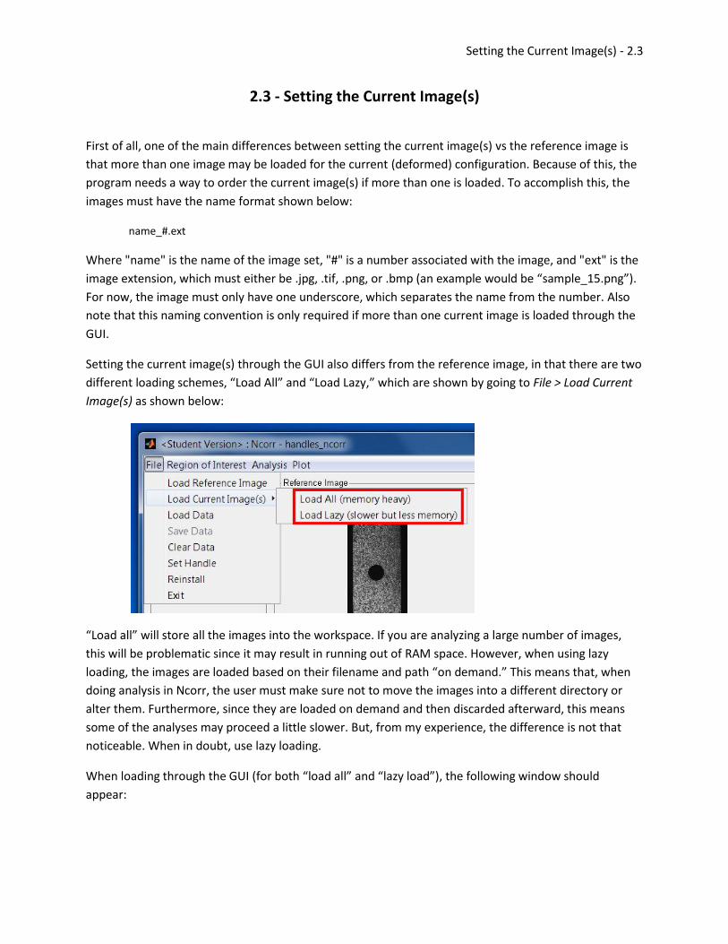
Setting the current image(s) through the GUI also differs from the reference image, in that there are two

different loading schemes, “Load All” and “Load Lazy,” which are shown by going to File > Load Current

Image(s) as shown below:

“Load all” will store all the images into the workspace. If you are analyzing a large number of images,

this will be problematic since it may result in running out of RAM space. However, when using lazy

loading, the images are loaded based on their filename and path “on demand.” This means that, when

doing analysis in Ncorr, the user must make sure not to move the images into a different directory or

alter them. Furthermore, since they are loaded on demand and then discarded afterward, this means

some of the analyses may proceed a little slower. But, from my experience, the difference is not that

noticeable. When in doubt, use lazy loading.

When loading through the GUI (for both “load all” and “lazy load”), the following window should

appear:


NOTE: Take note of the naming convention above. All of the current images follow the "name_#.ext" format, where name =

"ohtcfrp" and ext = "tif".

Simply drag and select all the current images of interest. For this example, the images with a post-fix of

“01” to “11” are selected).

Similar to the reference image, there is also an option to set the current image(s) directly through the

Ncorr handle. To do this, you can type "handles_ncorr.set_cur(data)" through the MATLAB terminal, as

shown below:

In the figure above, only a single current image is loaded, so it exists as a grayscale array of type double,

uint16, or uint8. To load more than one image, each current image gray scale array must be stored

together in a cell array. Furthermore, the ordering specified in the cell array is the order that Ncorr uses

to sort the images.

After the current images are uploaded, there are buttons on the bottom right of the Ncorr GUI which

become enabled and allow you to scroll through the images as shown below:


The current images should be ordered properly according to their number, and the last image in the

sequence will appear initially by default. It’s a good check to scroll through them to ensure the order is

correct.

Setting the Region of Interest - 2.4

2.4 - Setting the Region of Interest

There are three ways to set the region of interest (ROI); two are through the GUI and one is through the

MATLAB terminal. The most important thing to note here is that the ROI should be an array of the same

size as the reference image or current image (this depends on which type of analysis is done, which is

explained in greater detail in later sections. For this example, the ROI is set with respect to the reference

image). Furthermore, white regions represent the ROI, and black regions are outside the ROI. It is also

recommended to leave a black border near the boundary of the image, although the ROI used in the

example doesn’t, in order to illustrate a couple points.

Sample ROI

Load ROI: The first way to set the ROI is to load it from an image by going to: Region of Interest > Set

Reference ROI and then pressing the Load ROI button. This is the recommended way to set a ROI

because you can use a program like Photoshop to accurately trace an outline of the sample in order to

obtain the best ROI. The only problem with this method is that it can be tedious. Anyway, a gui should

appear as shown below:

For the example used in this user guide, this form of setting the ROI is used.


Draw ROI: The second way to set the ROI is to draw the ROI directly in MATLAB by using Region of

Interest > Set Reference ROI and then pressing the Draw ROI button. This is the preferred method for

preliminary analysis because it can be done quickly. An example ROI is shown below and was

constructed using "+ Poly" followed by "- Ellipse," where the "+" prefix indicates adding portions to the

ROI; "-" subtracts regions:

NOTE: The green shapes represent regions which add to the ROI, red shapes represent regions that subtract from the ROI, and

blue shapes represent regions which are active (i.e clicked on)

To obtain better precision when drawing ROIs, you can zoom and pan the view. Zooming can be enabled

by clicking the zoom button once and disabled by clicking it again (or by clicking a different button, such

as adding a region or pressing the pan button). An example is shown below:

It is also possible to delete specific shapes by right clicking them and selecting "Delete," as shown below:


MATLAB Terminal: Once again, similar to loading the reference and current image through the MATLAB

terminal, typing "handles_ncorr.set_roi_ref(data)" will set the ROI using the 2D array "data.” Note that

data must be of type logical. An example is shown below:

Setting DIC Parameters - 2.5

2.5 – Setting DIC Parameters

The DIC parameters can be set by going to Analysis > Set DIC Parameters. The DIC analysis used in this

program is based off of Bing Pan's RG-DIC framework. RG-DIC is highly robust and computationally

efficient as well. More details can be found in Bing Pan's paper on RG-DIC as well as the "DIC

Algorithms" section on the ncorr.com website.

A GUI should appear as shown below:

NOTE: A subset spacing of 3 is shown above to better illustrate the spaced points on the zoomed in subset, but for the example

analyzed in this manual, a subset spacing of 1 was used to obtain higher resolution results.

There are several key components to this GUI. The first is obviously the menu on the left, but it is also

important to note that the subset preview is interactive. A green impoint (highlighted by a red square) is

placed in the axes labeled "Subset Location." This point is draggable and is the center point of the subset

shown on the right. The subset on the right gives an idea of what the subset spacing (space between the

two dots within the red squares) and subsets will appear like. It's important to note that these

highlighted points are where the subset locations will be, and not part of the speckle pattern in the

uploaded image. An explanation of the menu components are given below:

Subset Options: These options are the main components of DIC analysis. They dictate how large the

subsets should be and the spacing between them. The spacing component is purely for reducing

computational load. There are defaults for both options, but it's up to the user to select the most

optimal settings. The most important option to get correct is the subset radius. There is an abundance of

literature available for the selection of the subset size, as well the effects of subset size on DIC analysis,

Setting DIC Parameters - 2.5

but most of the conclusions from these studies are often based on heuristics and empirical observations.

Overall, the main idea is to select the smallest subset possible which does not result in noisy

displacement data (as larger subsets tend to have a smoothing effect). Some iteration may be required

to get this option right.

Iterative Solver Options: The iterative solver used in the DIC analysis is the inverse compositional image

alignment technique (A good paper on this topic is Baker et al and Bing Pan's paper on his adaptation for

this technique for DIC). The exit criteria for this iterative solver are the norm of the difference vector as

well as the number of iterations. The default options for the iterative solver are actually pretty strict, but

they can be relaxed if faster analysis is desired by reducing the iteration number cutoff as well as

increasing the norm of the difference vector cutoff.

Multithreading Options: Ncorr has the ability to use multithreading to speed up the computation

process. The default number of threads is the number of cores specified by the user during installation,

although I have left the option to alter this number again through this GUI.

High Strain Analysis: In the example used specifically in this section, high strain analysis is not required.

However, the high strain analysis works by updating the reference image (as well as the ROI) and then

“adding” displacement fields together. If you enable this parameter, there are two different ways the

updating can proceed: In the case of the “seed propagation” option, the reference image will be

updated based on the correlation coefficient and the number of iterations to convergence of the seeds.

If these exceed a certain heuristic threshold, then the reference image will be updated. For the “leap

frog” approach, the user can manually select how many images to use before updating the reference

image. For both options, if the “automatic propagation” checkbox is checked, then the seeds will be

placed automatically for the updated reference image based on their previous displacements and the

DIC analysis will proceed automatically until completion. If this is unchecked, then the user will have to

replace the seeds manually every time the reference image is updated.

Discontinuous Analysis: For this example, discontinuous displacements are not anticipated, so this

feature isn’t used. Regardless, subset truncation is a feature that prevents subsets from wrapping

around a crack tip which can cause distortions near the cracktip. This feature is elaborated on in the

discontinuous displacements section.

DIC Analysis - 2.6

2.6 – DIC Analysis

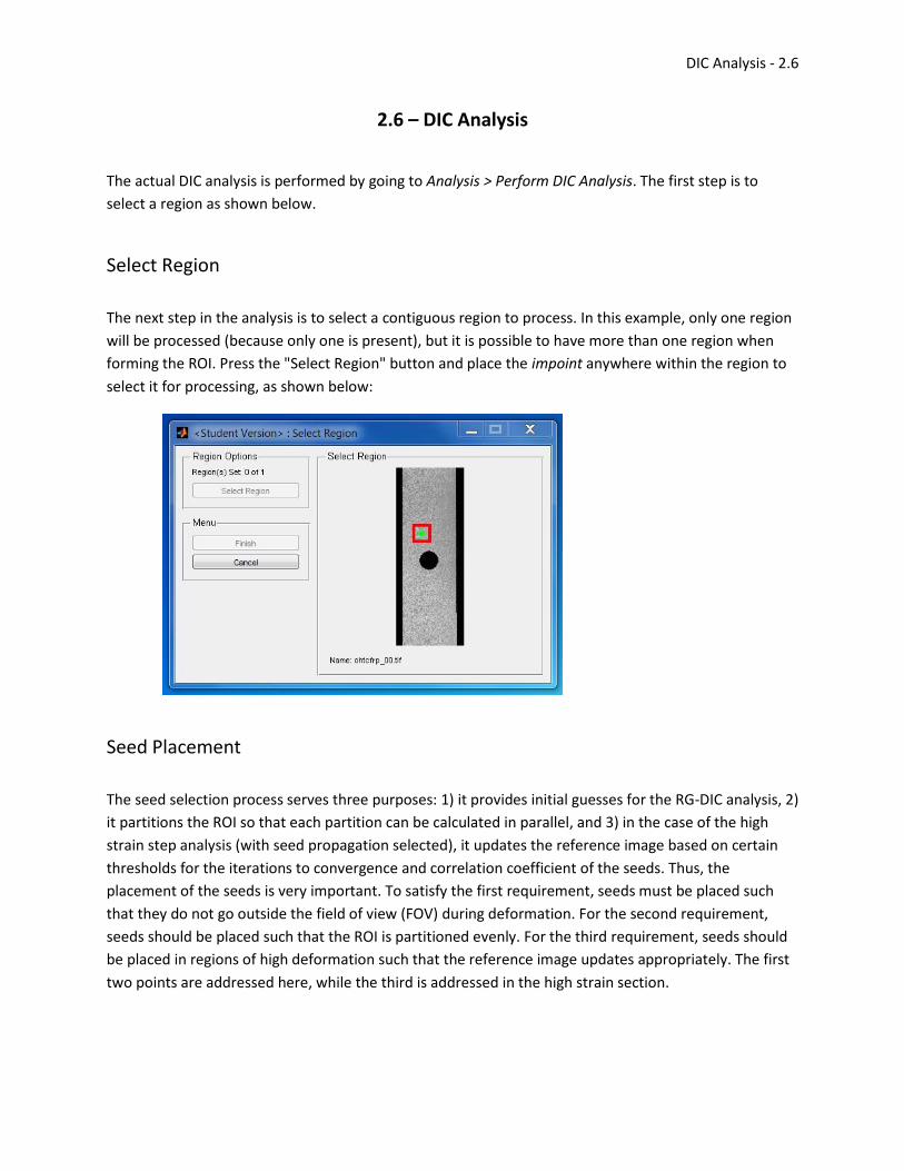
The actual DIC analysis is performed by going to Analysis > Perform DIC Analysis. The first step is to

select a region as shown below.

Select Region

The next step in the analysis is to select a contiguous region to process. In this example, only one region

will be processed (because only one is present), but it is possible to have more than one region when

forming the ROI. Press the "Select Region" button and place the impoint anywhere within the region to

select it for processing, as shown below:

Seed Placement

The seed selection process serves three purposes: 1) it provides initial guesses for the RG-DIC analysis, 2)

it partitions the ROI so that each partition can be calculated in parallel, and 3) in the case of the high

strain step analysis (with seed propagation selected), it updates the reference image based on certain

thresholds for the iterations to convergence and correlation coefficient of the seeds. Thus, the

placement of the seeds is very important. To satisfy the first requirement, seeds must be placed such

that they do not go outside the field of view (FOV) during deformation. For the second requirement,

seeds should be placed such that the ROI is partitioned evenly. For the third requirement, seeds should

be placed in regions of high deformation such that the reference image updates appropriately. The first

two points are addressed here, while the third is addressed in the high strain section.

DIC Analysis - 2.6

An example of unappropriate/appropriate seed placements for the example image is shown below:

These seed positions are not preferable because the regions aren't evenly sized and they aren't nice "full" shapes.

These seed placements are more preferable because the regions are evenly sized and have nice "full" shapes.

After the seed placement is done, a preview will appear. It's import that the user checks the seeds

through this GUI because it's possible that the seeds can be processed incorrectly. The main reasons for

seeds being incorrect can be either through a failure in convergence (this rarely happens as long as there

are no large rotations or deformations present), or if the seeds travel outside the current image as the

sample deforms. An example for proper seed preview is shown below:

DIC Analysis - 2.6

Notice that all the seed locations in the reference image seem to match appropriately with the locations

in the current image. Furthermore, the reference subset and transformed current subsets look very

similar. Lastly, the number of iterations to convergence was way below the cutoff, and the relatively low

correlation coefficient both imply a good and correct seed placement.

As mentioned before, it's possible for seeds to travel outside the image during deformation which

results in improper seed calculations. Because this is actually a somewhat common occurrence

(especially when the whole sample cannot be imaged within the field of view), an example is given

below with tips on how to catch this mistake and correct it:

DIC Analysis - 2.6

Suppose for instance that the seeds are placed as shown above. It turns out that the sample in the

picture undergoes some translation upwards as it deforms. The seed highlighted in red actually goes

"out of the picture" in some of the current images. In this case, an error message will generally display

that notifies the user of a seed point with a high correlation coefficient value. This is an important

indicator of a seed that has possibly been processed incorrectly. You can confirm this by viewing the

seed preview below:

All of the highlighted things in the figure above indicate potential problems. In the location pictures, it

becomes evident that the location of the top seed in the current image is completely off, whereas the

other three seeds are correct. Visual inspection of the enlarged reference and current subsets also show

that they look very different. Lastly, the maximum number of iterations (50 for this case) was used

before convergence was reached; this is typically another good indicator of an improperly calculated

seed. The solution here is to move the seed to a lower location or potentially redraw the ROI to exclude

the top region.

Anyway, after the seeds have been properly placed and calculated, the RG-DIC analysis will run until

completion. The next step in the process is to format the displacements.

Formatting Displacements - 2.7

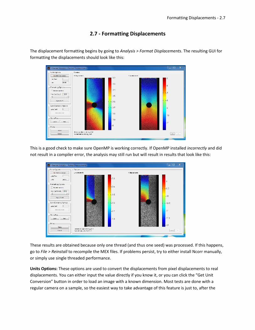
2.7 - Formatting Displacements

The displacement formatting begins by going to Analysis > Format Displacements. The resulting GUI for

formatting the displacements should look like this:

This is a good check to make sure OpenMP is working correctly. If OpenMP installed incorrectly and did

not result in a compiler error, the analysis may still run but will result in results that look like this:

These results are obtained because only one thread (and thus one seed) was processed. If this happens,

go to File > Reinstall to recompile the MEX files. If problems persist, try to either install Ncorr manually,

or simply use single threaded performance.

Units Options: These options are used to convert the displacements from pixel displacements to real

displacements. You can either input the value directly if you know it, or you can click the “Get Unit

Conversion” button in order to load an image with a known dimension. Most tests are done with a

regular camera on a sample, so the easiest way to take advantage of this feature is just to, after the


experiment in complete, replace the sample with a ruler so you can get an idea of what the units are. An

example of the GUI is shown below:

For this sample set, I’m actually not sure what the unit to pixel conversion is, so I’ve left this option as

the default for the rest of the user guide. But, just for the sake of an example, assume the undeformed

sample is 10 mm wide. You can apply this knowledge by loading the reference image through “Load

Calibration Image” and then setting a line across the sample with “Set Line.” Lastly, the units, mm, and

the number of units, 10, can be set in their appropriate boxes. Assuming the sample is 10mm wide, this

will apply the correct conversion to convert the displacements from pixels to mm (determined to be

0.031791 mm/pixel in this case). It’s important to note that this assumes pixels are square, which is

usually the case.

Formatting Options: These options help filter out “bad” data points. In the example done in this section,

some of the points in the ROI travel outside the FOV. These points can be filtered out by reducing the

correlation coefficient cutoff. In conjunction with this, the locations of the min and max displacement

values can assist in this analysis, as “bad” data points generally have very high or very low values. A good

cutoff for the example done in this guide is to set the correlation coefficient cutoff to 0.02 (which was

applied to all images), as shown below:


Note that the preview above was zoomed in using the zoom/pan options. The filtering out of bad data

points is shown below:

Lens Distortion Options: This is an option to correct for errors involving radial lens distortion. The

distortion correction follows from eq.6 in “Systematic errors in two-dimensional digital image

correlation due to lens distortion,” except the coefficient’s sign is flipped to make it positive in general.

The correction is applied assuming the distortion center is at the center of the image; this might not

always be true but is usually a reasonable assumption. If no calibration tests have been done or you’re

unsure what the lens coefficient is, then just leave it as 0.

As of now, a lens coefficient can only be applied. Bing Pan provides a method for determining the lens

coefficient, but I have yet to integrate this into Ncorr. The process basically requires DIC analysis to be

run on images taken during rigid body translation tests and then performing a simple least squares

analysis to solve for the lens distortion parameter. In future revisions of the program, I may implement

this feature.

Strain Analysis - 2.8

2.8 - Strain Analysis

The strain analysis begins by going to Analysis > Calculate Strains. The strains are calculated from the

displacement data by using a least squares plane fit to a local group of data points (in this case a

contiguous circle) which is based on Bing Pan's work on strain calculation. The displacements gradients

are then found from the plane parameters; these gradients are used to calculate Green-Lagrangian and

Eulerian-Almansi strains. A more detailed description is given in the "DIC Overview" section on the

ncorr.com website.

Strain Options: The only parameter you can vary here is the strain radius. This is the radius of a circle

which selects a group of points to fit a plane to. A preview is provided so the user can visualize the plane

fitting. The selection of the ideal strain radius is similar to the selection of the ideal subset radius, in that

the smallest radius is desired which does not result in noisy strain data. The default radius is set to 15,

but it is up to the user to select the most optimal radius for their data.

The impoint highlighted in the red box is draggable, and updates the plane fit shown on the right side.

The recommended way to use this analysis is to drag the point to areas of high displacement gradients

and view if the curve fit is still reasonable. For this example, I've placed the point near the max

displacement values and reduced the strain radius until a good plane fit was obtained as shown below:

Visually, it appears the strain radius is too large for this displacement field.

Strain Analysis - 2.8

Reducing the strain radius to a value of 5 appears to give a much better fit for the plane. In this example, this value is used to generate the strain field.

In future revisions, I may add other metrics (such as R2 values) to assist in the strain radius size selection.

Lastly, the strain radius should be selected with regards to the last current image (which is shown first

by default), as this image will most likely have the highest displacement gradients.

View Options: These dropdown menus allow you to switch from the U-displacements to the V-

displacements and vice versa. They also allow you to switch from the Lagrangian to the Eulerian

perspective. By default, both Green-Lagrangian and Eulerian-Almansi strains are calculated.

Discontinuous Analysis: Just like for DIC, there is also an option to utilize subset truncation for the strain

calculations. This feature prevents subsets from wrapping around a crack tip which can cause

distortions near the cracktip. This feature is elaborated on in the discontinuous displacements section.

Plotting - 2.9

2.9 - Plotting

At this point, it is assumed either the displacements have been formatted or the strains have been

calculated. Plotting can be achieved by going to Plot > View Displacement Plots or Plot > View Strain

Plots from the main Ncorr GUI. This is the last step of the analysis. An example of the plots used in the

examples in this user guide is shown below:

There are a couple basic features available, the first one being that the plot windows are resizable. They

are the only GUI windows in Ncorr that are resizable at the time of writing this manual. Furthermore, if

you hover your cursor over the data, a data cursor appears that informs you of the displacement or

strain data at that location, as shown below:

NOTE: From my experiences working with the plotting tool on different operating systems and versions of MATLAB, there

appear to be inconsistencies between versions with regards to the stacking order of objects (i.e. sometimes the scalebar/axes

appear behind the data if a contour plot is present), but I tried to optimize it for Windows on version R2012a. If the axes,

scalebar, and contour plot are disabled, the plot appears to work fine on all versions of MATLAB I've tested Ncorr on.

Local Plot Options: These options are pretty self-explanatory. The only thing to note here is that these

options only affect the plot that is being adjusted (as opposed to other options which affect all open

plots). Furthermore, the transparency option is disabled when the contour plot is enabled. This is

because transparency does not work well with the contour plot. In general, the contour plot does not

work that well with strain plots because strain plots are generally noisier than displacement plots which

results in jagged contours.

Plotting - 2.9

View Options: Once again, these options are pretty self-explanatory. These allow you to switch between

Lagrangian and Eulerian perspectives. For strains, these will switch between Green-Lagrangian strains

and Eulerian-Almansi finite strains tensors. This option will affect all open data plots.

Scalebar Options: This affects the visibility and length of the scalebar (displayed in the bottom-left of

the plot). This option will affect all open data plots.

Axes Options: This option affects the visibility of the axes (displayed in the top-left of the plot). This

option will affect all open data plots.

Saving the Figure: A figure can be saved by going to File > Save Image > Save Image Without Info, File >

Save Image > Save Image With Info, or File > Save Gif within the plot window. This will allow you to save

nice figures for publications, websites, or any other purpose. In this guide, I will focus on saving images,

as the animated gif option is more useful for high strain calculation (which is discussed in the high strain

section) because it generally involves many images. After selecting the save image option, a menu with a

preview should appear as so:

This will allow you to resize the image if you desire. Please note that if a large spacing parameter is used,

the image may look blurry if you upsize it because the image and data plot must be the same size when

plotting in MATLAB. The best solution for this would be to rerun the analysis with a smaller subset

spacing parameter. Also, I recommend saving the figure as a .tif because MATLAB appears to compress

other image formats which may lead to a loss of quality.

Directly Obtaining and Altering the DIC Data - 2.10

2.10 - Directly Obtaining and Altering the DIC Data

The DIC data can be accessed directly through the "handles_ncorr" handle. For example, by typing

"handles_ncorr.data_dic" into the MATLAB terminal, you can access the data structure that contains the

strain and displacement data as shown below:

Notice that both "dispinfo" and "straininfo" only have one element. This is because they contain

parameters which are consistent over the entire analysis. On the other hand, both "displacements" and

"strains" have eleven elements. This is because these fields contain information specific to each current

image. For the example used in this section, we have uploaded eleven current images, which correspond

to eleven elements seen above.

The size of the displacement/strain plots themselves depend on the reference image and the subset

spacing utilized. For the general case, the size of the displacement/strain plot will be:

size(reference(1:1+subsetspacing:end,1:1+subsetspacing:end))

where "reference" is the 2D reference image grayscale array and "subsetspacing" is the subset spacing

parameter (where a value of 0 results in no reduction). For example, if a reference image of size

400x1040 and a subset spacing of 1 is used (as is done in the example in this manual), then the

displacement/strain plot size will be 200x520.

The displacements with respect to the reference configuration (Lagrangian) are stored in the plots with

the "_ref" suffix. The "_cur" suffix is used for displacements with respect to the current configuration

(Eulerian).

For easy reference, each field of "handles_ncorr.data_dic" will be explained in a table format as shown

below:

handles_ncorr.data_dic.displacements

Field Explanation plot_u_dic Plot containing U displacement data WRT the updated reference image (based on imgcorr)

after DIC analysis

plot_v_dic Plot containing V displacement data WRT the updated reference image (based on imgcorr) after DIC analysis

plot_corrcoef_dic Plot containing correlation coefficient data WRT the updated reference image (based on imgcorr) after DIC analysis

roi_dic ROI corresponding to valid displacement data WRT the updated reference image (based


on imgcorr) after DIC analysis

plot_u_ref_formatted Plot containing U displacement data WRT the reference configuration after it has been formatted

plot_v_ref_formatted Plot containing V displacement data WRT the reference configuration after it has been formatted

roi_ref_formatted ROI corresponding to formatted displacement data WRT the reference configuration

plot_u_cur_formatted Plot containing U displacement data WRT the current configuration after it has been formatted

plot_v_cur_formatted Plot containing V displacement data WRT the reference configuration after it has been formatted

roi_cur_formatted ROI corresponding to formatted displacement data WRT the current configuration

handles_ncorr.data_dic.dispinfo

Field Explanation type String representing whether “regular” or “backward” analysis was done; this value can

either be 'regular' or 'backward'

radius Integer representing the subset radius

spacing Integer representing the subset spacing

cutoff_diffnorm Number representing the cutoff for the norm of the difference vector in the inverse compositional method

cutoff_iteration Integer representing the cutoff for the maximum number of iterations allowed for the inverse compositional method

total_threads Integer representing the total number of threads specified during the RG-DIC parameter specification stage (can be different than the number of cores specified during installation)

stepanalysis Structure containing data for the step analysis. The fields “enabled”,”type”, “auto”, and “step” represent if the step analysis is enabled, whether seed propagation or leapfrog is used, whether seeds will automatically get placed at each step, and the step parameter for the leapfrog analysis, respectively.

subsettrunc Logical parameter specifying if subset truncation was used for the RG-DIC analysis.

imgcorr Structure containing the image correspondences for the step analysis. For each element, there is an “idx_ref” and “idx_cur.” The idx’s are zero based and assume the reference and current images are concatenated. idx_ref is the index for the updated reference image whereas idx_cur is the index of the last current image WRT this reference image.

pixtounits Number representing the conversion between pixels to real units. In the form of units/pixels.

units String containing the units

cutoff_corrcoef Number representing the minimum correlation coefficient value allowable for displacement datapoints corresponding to a dataplot.

lenscoef Number representing the radial lens distortion coefficient

handles_ncorr.data_dic.strains

Field Explanation plot_exx_ref_formatted Plot containing the Exx Green-Lagrangian strains (WRT the reference image)

plot_exy_ref_formatted Plot containing the Exy Green-Lagrangian strains (WRT the reference image)

plot_eyy_ref_formatted Plot containing the Eyy Green-Lagrangian strains (WRT the reference image)

roi_ref_formatted Object containing the ROI information for valid points after strain calculation (It's possible for some points to be removed during strain calculation for regions that do not have enough points to form a plane fit)

plot_exx_cur_formatted Plot containing the Exx Eulerian-Almansi strains (WRT the current image)

plot_exy_cur_formatted Plot containing the Exy Eulerian-Almansi strains (WRT the current image)


plot_eyy_cur_formatted Plot containing the Eyy Eulerian-Almansi strains (WRT the current image)

roi_cur_formatted Object containing the ROI information for valid points after strain calculation (It's possible for some points to be removed during strain calculation for regions that do not have enough points to form a plane fit)

handles_ncorr.data_dic.straininfo

Field Explanation radius Integer representing the strain radius

subsettrunc Logical parameter specifying if subset truncation was used for the strain analysis.

Lastly, any information that the user wants to alter should be copied first to another variable in the main

workspace. By default, the properties of Ncorr are set to "(SetAccess = private)" to prevent inadvertent

alteration of data. If the user wants to alter the data directly, then the user can go into the ncorr.m

source code and change "(SetAccess = private)" to "(Access = public)" to alter these properties directly

as shown below:

It may be possible to crash Ncorr by setting inconsistent data and thus caution is advised if going this

route.

High Strain DIC Analysis - 3.1

3.1 – High Strain DIC Analysis

For this section, it is assumed the program has already been installed and the user has already read the

General DIC section. The images used for this section (the “weld” sample from SEM’s DIC challenge) are

available off the Ncorr website if the user would like to follow along:

http://ncorr.com/download/sample13.zip

Start by setting the reference image to the first image (post fix of “000”) of the set. Next, load the

current images by using “Lazy Load” (or potentially “Load All” if your computer has a lot of RAM) and

selecting all the images from postfix of “020” until the postfix of “910” (note that at “915” the sample

has failed- so omit this picture) as the current images. Lastly, set the reference ROI to the ROI provided

in the image set (named “roi.tif”). If successful, the GUI should appear as below:

Now, if the user simply proceeds as is done in the general DIC section, he/she will find that the seeds for

the latter images will always be incorrect. This is because this sample undergoes very high deformation.

The underlying problem here is that the pattern between the reference image and the last current

image changes so much that the matching algorithm no longer works. This type of sample requires the

reference image to be updated. To account for this, the high strain step analysis needs to be enabled

when setting the DIC Parameters, which is discussed in the next paragraph.

For high strain DIC, it’s recommended to set the type of step analysis to “seed propagation” with the

“automatic propagation” checkbox enabled, as shown below:


There are a couple things to note here. First of all, there are a large number of images involved in this

analysis, so performance issues will be a concern. To increase the speed of the analysis, I’ve elected to

increase the subset spacing to 6. Furthermore, the norm of the difference vector has been increased to

10-3 and the iteration cutoff has been set to 20. These will reduce the number of material points to

analyze and also make the conditions on the iterative solver more relaxed. The effects of doing these

two things will be a lowered resolution in the acquired displacement field, and a slightly reduced

accuracy as well. If time permits, then the spacing, norm of difference vector, and iteration cutoff can be

left to their default values.

In addition, the high strain analysis has been enabled with the seed propagation and automatic

propagation parameters enabled. This allows the program to automatically update the reference image,

as well as to automatically place seeds so the analysis can proceed in an automated fashion until

completion. If “leapfrog” is selected, then the reference image will update according to whatever step

number is provided. Lastly, if auto propagation is disabled, then the user will have to manually place the

seeds every time the reference image is updated. This can be quite tedious, but also ensures the seeds

are correct, so this option should only be disabled if you want to ensure completely that the seed

placements are correct.

The next crucial step is the seed placements. Recall from the general DIC analysis that there are two

main considerations for seed placement for the regular DIC analysis. First of all, they need to be placed

on a material point that does not exit the FOV as the sample deforms. Next, they need to be placed such

that the regions are more or less evenly portioned so they can be calculated nicely in parallel. For high

strain analysis with seed propagation, there’s another consideration: since the reference image is


updated based on the correlation coefficient and number of iterations to convergence of the seed

points, they need to be placed in a region of high deformation, so that the reference image updates

correctly. If you examine the last current image in the example set, you’ll see that the region of highest

deformation is near the region circled below:

Basically, from inspection of the last current image (shown on the left), you can assume the highest

deformation occurs approximately in the region encircled by the red ellipse (where the crack initiates). It

would be ideal to place the seed points on the reference image corresponding to this region so that the

reference image updates properly. With this in mind, the seeds are placed as so:

These seed locations (shown in the red boxes) satisfy the three requirements explained previously.

Clicking finish yields the following seed preview screen:


The most important thing to note here is that the last image seeded is not the last image of the series.

The image with postfix “180” was determined to be the last properly seeded image of the series (Note

that this can vary; it’s possible the image can be a couple before or after this one depending on the seed

placement). This image will serve as the updated reference image until it is updated again. Click finish to

proceed with the analysis. It should continue until completion.

Before continuing, I’d like to explain what exactly is going on “under the hood.” Basically, every time the

reference image gets updated, the seeds are automatically “propagated” and placed as the analysis

proceeds. Additionally, the ROI is also updated based on the displacements on the boundary of the ROI.

For this example, the updated thread diagrams with seed placements are shown below:


For this particular example, there were four updates. The ROIs and seed positions are automatically

updated (shown as red circles) and then subsequently processed. The corresponding “imgcorr”

structures are also superimposed as an example for how this structure works.

From here, the only problem is that the displacement fields are now going to be with respect to the

updated reference image. The next step is to somehow “add” them in order to bring them all back to

the Lagrangian perspective (i.e with respect to the original reference image). This step is taken care of

when the displacements are formatted. The formatting displacements GUI should look similar to the one

shown below:

A couple things to note here: first of all, near the top of some of the displacement fields, the data

appears to be very poor. This is because these material points travel outside the FOV as the sample is

deforming, so these points need to be removed. Furthermore, a crack develops in the sample. This

means points near this crack are also poorly analyzed, so they should be removed as well. Empirically, it

appears that setting a correlation coefficient cutoff of 1 yield good results:


One last thing to point out is that the reference name shown above (near the bottom left) refers to the

updated reference image.

The last step of the analysis is to calculate the strains. A strain radius of 7 appears to give good results as

shown below:

In terms of plotting, the only distinction to really make between high strain and regular DIC analysis is

that the user might want to consider saving an animated gif instead of regular pictures since so many

data plots are available. In this particular case, the Eulerian perspective makes for especially good

animations. Furthermore, it’s usually appropriate to set the same upperbound and lowerbounds for

strain in all the plots.

First, a plot for Eyy is shown below:


In order to set all the bounds for the strains the same, it’s necessary to set them such that the bounds

accommodate all plots. For this example, the lowerbound must be set near zero as shown below:

If this lowerbound is set any higher, it might result in an earlier plot becoming completely saturated. If

you do this, an error message will appear. Furthermore, I tend to add or subtract 0.0005 from the

bounds to guarantee the tick marks appear on the top and bottom of the colorbar as well, as shown

above. Anyway, after hitting “applying to all”, select File > Save GIF which will bring up the following

GUI:


Notice that, in addition to the size, you can also modify the time delay between animation frames. From

my experience, a time delay of 0.04 (25 fps) seems to work well for this data set, but the user can always

opt to increase it in order to slow the animation down and vice-versa.

Discontinuous Displacements DIC Analysis - 4.1

4.1 – Discontinuous Displacements DIC Analysis

For this section, it is assumed the program has already been installed and the user has already read the

General DIC section. The images used for this section (called the “crack sample”) are available off the

Ncorr website here if the user would like to follow along:

http://ncorr.com/download/cracksample.zip

For this analysis, images from my lab are going to be used. Furthermore, to demonstrate some of the

features of Ncorr, they will be loaded through the object handle instead of the GUI. The images were

taken from a high resolution CCD camera and are thus quite large. To account for this, I’ve decided to

read them through a script and then downsize them before loading them into Ncorr. The script is

included with the images but is also show below:

%% Open Ncorr handles_ncorr = ncorr;

%% Set Parameters % Load Ref ref = imread('ref.TIF'); ref = imresize(ref,0.5,'bicubic','Antialiasing',true);

% Load Cur cur = imread('cur.TIF'); cur = imresize(cur,0.5,'bicubic','Antialiasing',true);

% Load mask mask = rgb2gray(imread('mask_half.TIF')); mask = logical(mask(1:end,1:end));

% Set images handles_ncorr.set_ref(ref); handles_ncorr.set_cur(cur); handles_ncorr.set_roi_cur(mask);

The GUI should appear as so if everything went correctly:


The important thing to note is that the ROI was set with respect to the current image (i.e. it uses

“handles_ncorr.set_roi_cur(data)”). This is the key point to how Ncorr handles discontinuous

displacement fields. The idea is that the discontinuities are clearly visible in the current configuration.

The general process is that the ROI and DIC analysis proceed with respect to the current configuration,

and then an Eulerian to Lagrangian algorithm converts the displacements back to the reference

configuration. The ROI was traced around the crack in Photoshop; a close up of the ROI superimposed

on the current image is shown below:

The DIC parameters were then set as shown below:

The one thing to note in particular is that subset truncation is enabled. This prevents wrap around of

subsets around the crack tip. This is demonstrated below:


This demonstrates how subset truncation works. It truncates portions that will wrap around a crack tip.

This is useful because the shape functions are linear, whereas the deformation near the crack tip is

highly nonlinear. This helps prevent some distortions in the displacement fields which will be shown

later. Anyway, the seeds are placed as so:

After the analysis is complete, the displacement formatting does not need any special considerations.

Just accept the defaults as shown below:


For the strain analysis, also utilize subset truncation:

After everything is complete, the displacement and strain plots should appear as shown below (only the

V displacement and Eyy strains are shown below since the sample is loaded in the y direction):

I’ve taken the liberty of also performing the same analysis without subset truncation. Comparisons are

shown below between the V displacement field (top row) and Eyy strain field (bottom row) which

demonstrate the benefit of using subset truncation:

ncorrmanual_v1_2

Documents

Transcript of ncorrmanual_v1_2