NBER WORKING PAPER SERIES RATIONAL EXPECTATIONS, ThE ...
34
NBER WORKING PAPER SERIES RATIONAL EXPECTATIONS, ThE EXPECTATIONS HYPOTHESIS, AND TREASURY BILL YIELDS: AN ECONOMETRIC ANALYSIS David S. Jones V. Vance Roley Working Paper No. 869 NATIONAL BUREAUOF ECONOMIC RESEARCH 1050 Massachusetts Avenue Cambridge MA 02138 March 1982 The research reported here is part of the NBER's research program in Financial Markets and Monetary Economics. Any opinions expressed are those of the author and not those of the National Bureau of Economic Research.
Transcript of NBER WORKING PAPER SERIES RATIONAL EXPECTATIONS, ThE ...

NBER WORKING PAPER SERIES
RATIONAL EXPECTATIONS, ThE EXPECTATIONS HYPOTHESIS,AND TREASURY BILL YIELDS: AN ECONOMETRIC ANALYSIS
David S. Jones
V. Vance Roley
Working Paper No. 869
NATIONAL BUREAUOF ECONOMIC RESEARCH1050 Massachusetts Avenue
Cambridge MA 02138
March 1982
The research reported here is part of the NBER's research programin Financial Markets and Monetary Economics. Any opinionsexpressed are those of the author and not those of the NationalBureau of Economic Research.
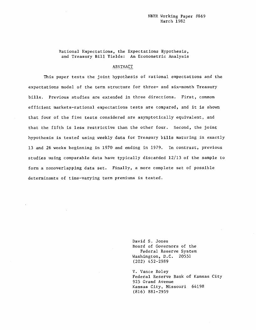
NBER Working Paper #869March 1982
Rational Expectations, the Expectations Hypothesis,and Treasury Bill Yields: An Econometric Analysis
ABSTRACT
This paper tests the joint hypothesis of rational expectations and the
expectations model of the term structure for three— and six—month Treasury
bills. Previous studies are extended in three directions. First, common
efficient markets—rational expectations tests are compared, and it is shown
that four of the five tests considered are asymptotically equivalent, and
that the fifth is less restrictive than the other four. Second, the joint
hypothesis is tested using weekly data for Treasury bills maturing in exactly
13 and 26 weeks beginning in 1970 and ending in 1979. In contrast, previous
studies using comparable data have typically discarded 12/13 of the sample to
form a nonoverlapping data set. Finally, a more complete set of possible
determinants of time—varying term premiums is tested.
David S. JonesBoard of Governors of the
Federal Reserve SystemWashington, D.C. 20551(202) 452—2989
V. Vance RoleyFederal Reserve Bank of Kansas City925 Grand AvenueKansas City, Missouri 64198(816) 881—2959

Revised
February 1982
RATIONAL EXPECTATIONS, THE EXPECTATIONS HYPOTHESIS,AND TREASURY BILL YIELDS: AN ECONOMETRIC ANALYSIS
David S. Jones and V. Vance Roley*
The joint hypothesis consisting of rational expectations and the
expectations model of the term structure has been subject to an increasing
amount of scrutiny in recent years. Some of this research has followed Roll
[26] and examined this joint hypothesis under the guise of the "efficient
markets" hypothesis. Other researchers have taken the study by Modigliani and
Shiller [18] as the starting point and tested rationality and the expectations
hypothesis explicitly. Prominent examples of recent studies focusing on this
model include McCulloch [13], Mishkin [14,15], Pesando [23], Sargent [27],
Shiller [28,29], Friedman [6], and Singleton [31,32], who either explicitly or
implicitly test this joint hypothesis. In virtually all of these studies,
however, not only are different "nonoverlapping" data sets employed, but the
tests themselves apparently are not uniform. For example, Mishkin [15] and
Sargent [27] test cross—equation restrictions implied by this theory, while
Pesando [23], Shiller [28,29], and Friedman [6] have collected data and utilized
tests that enable straightforward single—equation estimation.
As a whole, the evidence surrounding the validity of this joint hypothesis
is mixed. In cases where the potential roles of time—varying term premiums are
not explicit (e.g., Sargent [27] and Shiller [29]), the null hypothesis
associated with this model cannot be rejected. However, when time—varying
term premiums dependent on the level of interest rates are included, both
Shiller [28] and Friedman [6] reject the joint hypothesis. Moreover, in
studies allowing other possible determinants of time—varying term premiums,
Nelson [19] and Friedman [6] again reject the model. Still other researchers

—2—
have substituted alternative models of market equilibrium for the expectations
hypothesis and tested whether security markets are efficient (e.g., Fama {5]
and Mishkin [16]). In these latter studies, the expectations hypothesis is
rejected a priori.
The range of results from previous studies is attributable to at least
two factors. First, different data sets are used, some of which are constructed
more carefully than others. Second, the list of potential determinants of time—
varying term premiums has varied considerably among studies. Some might also
argue that a third possible reason for the divergent results is due to the
apparently different formulations of the tests. As is shown in the first sec-
tion of this paper, however, in tests using observed market data (as opposed
to the survey data used by Friedman [6]), many efficient markets—rational
expectations tests are asymptotically equivalent.
The purpose of this paper is to investigate the joint hypothesis of
rational expectations and the expectations model of the term structure in the
context of the Treasury bill market. This market is selected for two reasons.
First, the Treasury bill market has been studied extensively, with empirical
results that highlight the possible roles that data and methodology play in
tests of the model (e.g., Roll [26], Hamburger and Platt [10], Fama [5], Friedman
[6], and Mishkin [16]). Second, Treasury bill data are ideally suited for such
an exercise because (a) Treasury bills are issued at regular and frequent inter-
vals, (b) different maturities have homogenous tax treatment, and (c) they are
pure discount securities which avoids complications related to coupons. While
others have noted these attributes and investigated the behavior of Treasury
bill yields as a consequence, previous studies are almost uniformly based on

—3—
nonoverlapping quarterly samples that effectively discard 12/13 of the available
data. In contrast, in this paper all available data are used for Treasury bills
maturing in exactly 13 and 26 weeks in a sample spanning most of the l970s.
As Hansen and Hodrick [11] show in the context of the foreign exchange market,
more powerful asymptotic tests may be obtained using all of the available
weekly data than in constructing nonoverlapping samples to avoid the problem of
serial correlation.
Following this introductory section, the first section compares alterna-
tive tests of the joint hypothesis of rationality and the expectations hypoth-
esis. In the second section, the Treasury bill yield data used here as well as
the data for possible determinants of time—varying term premiums are described.
The estimation problems posed by the use of weekly overlapping data are also
discussed in this section. In the third section, the estimation and test
results are presented. The main conclusions of this paper are summarized in
the final section.
I. Tests of Rationality and the Expectations Hypothesis
In this section, five efficient markets—rational expectations tests
appearing in the literature are compared. Extending the results of Abel and
Mishkin [1], who show that Test I and Test II below are asymptotically equiva—
lent, two other tests may also be shown to be asymptotically equivalent to
Test I. In particular, it is demonstrated that a simple single—equation test
is in fact equivalent to more complicated tests involving restrictions across
equations.
In the discussion below, all derivations are in terms of the three— and
six—month yields which are examined empirically in a later section. Further—

—4—
more, it is assumed for analytical convenience that the data are nonoverlapping
in each case.-1 Under these conditions, the joint hypothesis of rational
expectations and the expectations model of the term structure may be repre-
sented by the usual approximation-'
R6t = (lI2).R3 + (l/2).E(R3t÷jQ) + a (1)
where
R6t = yield on six—month Treasury bills at time t
a = constant term premium (Hicks [121)
= information set used by investors at time t
E(... = expectation conditional on 2t' taken as the linearleast squares forecast of a random variable basedon information available at time t.
The above model (1) merely states that the yield to maturity on a six—month
Treasury bill equals one—half of the sum of the current three—month Treasury
bill yield and the expected three—month yield in period t+l evaluated at
time t, plus a constant term premium. Different permutations of the basic
relationship are used to derive the tests considered immediately below.
Test I
The first test considered here is taken as the standard when investigating
the asymptotic properties of alternative tests. This test is by far the easiest
to implement, and it follows directly from equation (1). In particular, the
hypothesis to be tested is that the expected quarterly holding—period yield
on a six—month Treasury bill differs from the current three—month Treasury bill
yield by at most a constant term premium. To conform to this test, equation
(1) may be rewritten as
hE(R6k) = R3 + a (2)
—5—
where
E(RtI)— E(R3+iI)
hR6 approximate holding—period yield on six—month Treasury
bills in period t (R = 2R6t—
In turn, the expression for the one—period—ahead three—month Treasury bill
yield may be represented as
R3t+l = E(R3+iIt) + e+1 (3)
where e+1 the forecast error for the three—month rate, is uncorrelated with
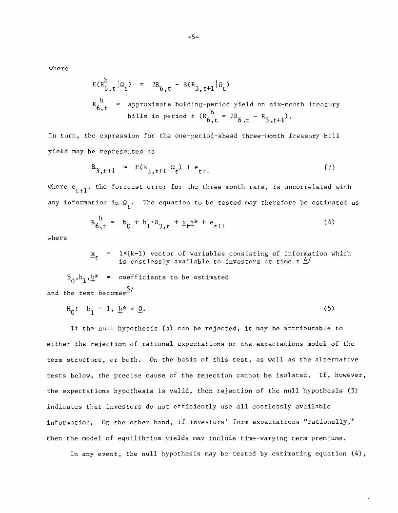
any information in The equation to be tested may therefore be estimated as
R611t = b0+ bi.R3 + + e1 (4)
where
= lx(k_l) vector of variables consisting of information whichis costlessly available to investors at time t
b0,b1,b* = coefficients to be estimated
and the test becomes—'
H0: b1=l,b=O. (5)
If the null hypothesis (5) can be rejected, it may be attributable to
either the rejection of rational expectations or the expectations model of the
term structure, or both. On the basis of this test, as well as the alternative
tests below, the precise cause of the rejection cannot be isolated. If, however,
the expectations hypothesis is valid, then rejection of the null hypothesis (5)
indicates that investors do not efficiently use all costlessly available
information. On the other hand, if investors' form expectations "rationally,"
then the model of equilibrium yields may include time—varying term premiums.
In any event, the null hypothesis may be tested by estimating equation (4),

—6—
or equivalently
Rt — R3 = + e+1
by ordinary least squares and computing the appropriate test statistic for
H0: b=O (5)
where
z = {R ,x }—t 3,t —t
= {b1_l,b*}and the constant term is assumed to be zero for simplicity. In this case,
the usual test statistic is
Q = b[a2(ZZ)']'b = (l/2)bZZb (6)
where b = (ZZ)1ZZ = NXk matrix with row j equal to z.,jl,. . .,N
y NX1 vector with element j equal to R . — R3 •,j1,. ..,N,J ,J
= [l/(N—k)](—Zb)(—Z).
As is well known, under the null hypothesis, Q has an F-distribution with (k,N—k)
degrees of freedom, and is asymptotically distributed as 2(k).
Test II
Another test formulated by Mishkin [15,161 involves cross—equation ratio-
nality restrictions. In this case, a distinction is made between anticipated
and unanticipated movements in economic variables following Barro [2,31. The
main feature of this framework is that if the economic variables in the model
are precisely those comprising the information set used by the market, then the
effects of unanticipated movements in variables on ex post holding—period yields
may be estimated, as well as testing the joint hypothesis of rational expecta-
tions and the expectations model of the term structure.
—7—
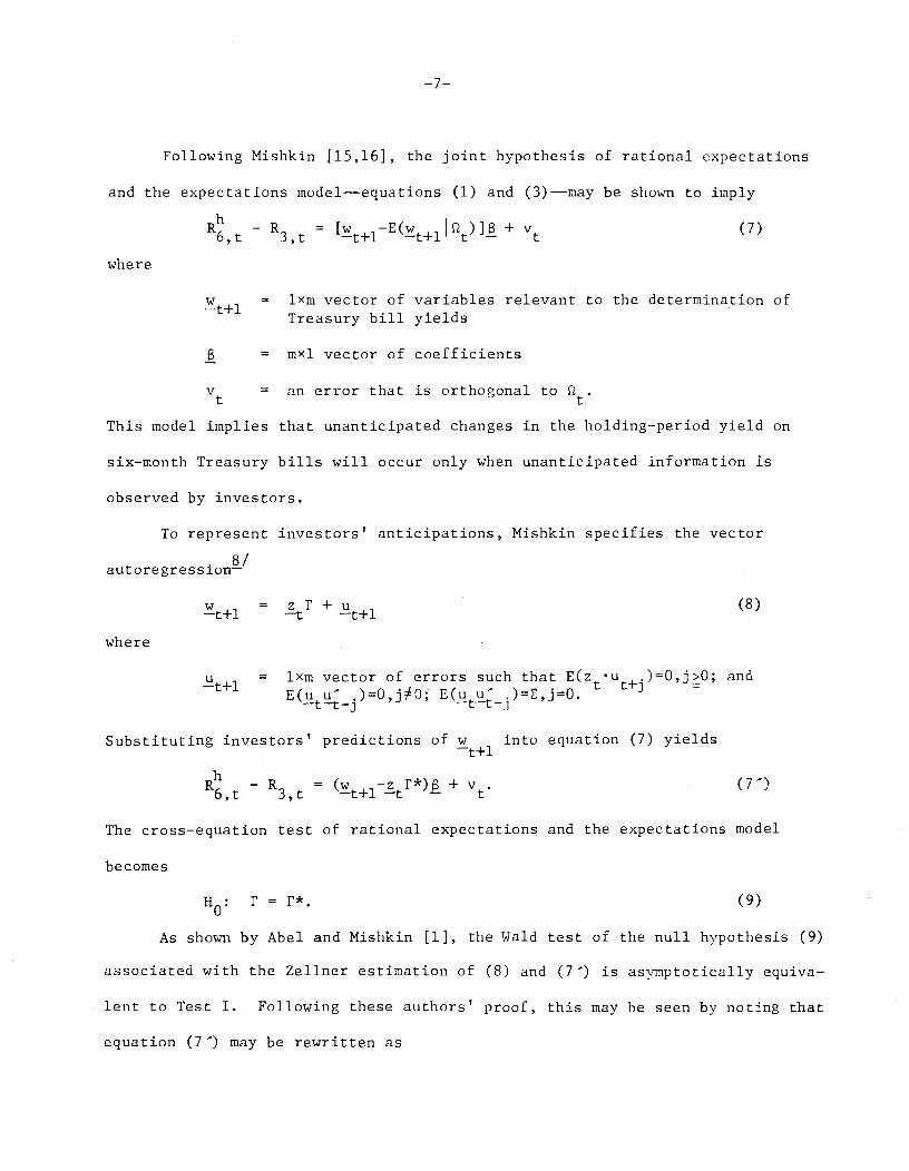
Following Nishkin [15,16], the joint hypothesis of rational expectations
and the expectations model—equations (1) and (3)—may be shown to imply
Rt - R3 = + v (7)
where
w+1
= lxm vector of variables relevant to the determination oft
Treasury bill yields
6 = mxl vector of coefficients
v = an error that is orthogonal to 2t t
This model implies that unanticipated changes in the holding—period yield on
six—month Treasury bills will occur only when unanticipated information is
observed by investors.
To represent investors' anticipations, Mishkin specifies the vector
8/autoregression—
w = zr+u (8)—t —t+l
where
u = lxm vector of errors such that E(z u .)=O,j>O; andt+l
E(uu .)E,jO.t 3 —
Substituting investors' predictions of w into equation (7) yieldst+l
Rt — R3t + Vt.
The cross—equation test of rational expectations and the expectations model
becomes
H0:r = r*. (9)
As shown by Abel and Mishkin [1], the Wald test of the null hypothesis (9)
associated with the Zeilner estimation of (8) and (7) is asymptotically equiva—
lent to Test I. Following these authors' proof, this may be seen by noting that
equation (7) may be rewritten as

—8—
—R3t = (w+i_zr) + + v (7)
where 0 = (r_r*)and the null hypothesis is
H0:0 = 0. (9)
Because the T constraint across equations (8) and (7) is not binding,
the Zeilner estimator of 3 may be obtained by estimating equations (8) and (7)
recursively using OLS. In the matrix notation used earlier, the OLS estimates
of equation (8) implies
zr= w— (10)
where W and U are NXm matrices corresponding to ;+l and u+1, respectively.Subutituting equation (10) into equation (7) yields
(7Becau;e the vector autoregression (8) is estimated by OLS, U is orthogonal to
Z and the estimator of 0 is
9 = (zz)z (11)
which is numerically identical to the estimator obtained in Test I.
The final step involves computing the Wald test statistic corre-
sponding to the null hypothesis (9). This statistic may be computed
as
R = 0{v(ZZ)1110 (12)
where ; = (l/N)(—u—ze)-(—u—ze)
which is asymptotically distributed as x2 with k degrees of freedom. Abel
and Mishkin {lJ further show that the v may be computed from the OLS estima-
tion of equation (4), and is equivalent, except for degrees of freedom, to

—9—
2 used in equation (12). Thus Test I—as described by equations (5) and
(6)—and Test Il—as described by equations (9) and (12)—are asymptotically
equivalent.
Test III
Another test involving cross—equation restrictions focuses on the forward
three—month Treasury bill yield and the time—series process generating the three—
month yield. In this respect, the rationality restrictions to be tested are
analogous to those specified by Modigliani and Shiller [18], and tested by
Pesando [21] and Friedman [7] with survey data for inflation and interest rates,
respectively.
Using the expression for the expectations hypothesis (1), the implied
three—month forward yield equals investors' rational expectation of the future
spot rate
2R6 — R3 =E(R3+1Jc2) (13)
where the constant term premium is again deleted without any loss of generality.
In turn, R3t+l is assumed to be generated by a stochastic process including all
available information at time t relevant to the determination of the equilibrium
yield
R3t+1 = + c1 (14)
where an error that is orthogonal to
The cross—equation test then involves the comparison of the estimated coeffi-
cients () in equation (14) with the estimated coefficients (*) in
2R6 — R3 + +1 (15)
where an error that is orthogonal to

—10—
That is, the null hypothesis is
H0:= :1*. (16)
that the right—hand side variables of equations (14) and (15) are
implying that the Zeilner and OLS estimators for this two—equation
equivalent. In matrix notation, these estimators may be written
as
[1 [(zz—1zU
H*J L
where = Nxl vector consisting of R3t+i,t=1,.. . ,N
£2 = Nxl vector consisting of 2 R6,_R3,ttl. . . ,N.
The variance—covariance matrix of these estimators is
I
V =
1*
where 011,012,a22 = consistent estimates of E(c),E(cfl), and E(),respectively.
In this case, it may be verified that the Wald test statistic for the
null hypothesis (16) is
R = [l/(o11+o22_2o12)](Ii*)(ZZ)(X_I*) (19)
which is asymptotically distributed as 2(k) under the null
hypothesis.
Alternatively, the stochastic processes (14) and (15) may be combined to
form
2R6t R3 — R3= + (20)
Note
identical,
system are
0 (zz)z][l1[2j
(17)
(18)

—11—
where 6 = kxl vector of coefficients
= an error that is orthogonal to
From equation (2), the left—hand side of equation (20) merely equals —R3t.
The OLS estimator of 6 may therefore be expressed as
6 = (zz)'Z (21)
with variance—covariance matrix
V(6) = a2(ZZ)' (22)
where a2 = OLS estimate of E(2).
Note that = 2 — which implies that equation (14) and (15) may be
substituted into (21) to yield
6 = (zz)z2 — (ZZ)z1 (23)
A similar substitution further implies that
a2 = + G2 — 2;2
where the a'. differ from a.. only with respect to degrees of freedom.1J 1J
Under the null hypothesis analogous to that in Test I (5), the relevant
test statistic for equation (20) is
R = [l/a2]6(ZZ)rS
= [l/(at1+a2_2a2) I (x_x*) (ZZ) (x_x*)
which is asymptotically equivalent to the Wald test statistic (19). The test
statistic for the cross—equation restrictions is, therefore, asymptotically
equivalent to that of the single—equation test described in Test I.

—12—
Test IV
In addition to using volatility measures to assess the joint hypothesis of
rational expectations and the expectations model of the term structure, Shiller
[29] also conducts formal econometric tests using a single—equation estimation
approach.-' In terms of the three— and six—month yields examined here, Shiller's
[29] single—equation approach involves estimating an equation of the form
R3+i — R6t =b0 + bi(R6 t-R3 + t+l (24)
where = an error that is orthogonal to
11/and testing the null hypothesis—
H0: b1 =1. (25)
To motivate this test, notice that from (1) investors' rational expec-
tation of the future three—month yield may be expressed in terms of available
yield data and a constant term premiunT"
E(R3+1c) 2•R6t —— (26)
Substituting expression (26) into (3) and then subtracting R6t from both sides
yields the expression
R3t+l — R6t = — + R6 — +e+1. (27)
From the above, it is apparent that a slightly more general representa-
tion of this same test may be formed by rewriting equation (24) as
R3t + R3 t+l — 2.R6 = b + b.R6 + bR3 + t+l (28)
and testing
H0: b = b 0. (25)
Further transformation of equation (28), using the definition of Rt provided

—13—
earlier, results in
-R3t
=—b
- b.R6t - b.R3t — t+i• (28)
This latter equation, together with the null hypothesis (25), is equivalent to
specialized version of Test I in which z consists of only R and R—t 6,t 3,t
Test V
The final case considered here is the test of cross—equation rationality
restrictions presented by Sargent [27].' In this test, cross—equation restric-
tions are tested for the vector autoregression.-'
in in
R =E a•R •+E bR3,t i 3,t—i . 6,t—i t
i=l i=l
(29)in m
R, =E cR •+E d•R +v6 t i 3,t—i. . i. 6,t—i ti=l i=l
where a,,b,c.,d. = coefficients to be estimated1 1 ] 1
u v = errors uncorrelated with R . and R ., for i>l,t' t 3,t—i 6,t—a. =
but possibly contemporaneously correlated.
The cross—equation restrictions are again derived from the approximation used
to represent the joint hypothesis of rational expectations and the expectations
model of the term structure, but in this case the model is specified in terms
of information known at time t—l
E(R6,k1_1) = (l/2).E(R3c1) + (l/2).E(R3,+1Ic2_1) + . (30)
As shown by Sargent [27], nonlinear restrictions on the vector autoregression
(29) are implied by this model (30).
As both Sargent [27] and Shiller [29] note, however, such complicated
nonlinear restrictions are not necessary if the data allow the computation of
forward rates. In particular, with the three— and six—month yields used here,

—14—
the expected three—month spot rate in period t may be expressed as
E(R3,l_1) = 2.R6,_i—
R3 t-l— ai (31)
where a under the null hypothesis. In turn, under the hypothesis of
rational expectations, the realizations of R3 and R6t may be represented as
R3+i = E(R3,+iQ_i) +
(32)
R6 = E(R6,Ict_1)+
where = an error that is orthogonal to t—l
= first—order moving_avrage error process, withorthogonal to
If the joint hypothesis is true, equations (31) and (32) may be substituted
into equation (30) to yield
(2.R6,_R3÷i) = (26,_i_R3,_1) + (c+1_2.n) (33)
where the left—hand side equals and the right—hand side consists of the
forward three—month rate corresponding to R3 and an error term.-' The ioint
hypothesis of rationality and the expectations theory of the term structure may
therefore be tested by estimating the equatiori-'1
=b.(2.R6,_i_R3,_i) + -—- +
(e+1—2.n) (3Y)
where l€Qt 1 and c is a vector of coefficients. The null hypothesis in this
case corresponds to the parameter restrictions
H: b = 1, c 0, (34)
which are a subset of the restrictions tested in the previous four tests.
To demonstrate that the restrictions given by the null hypothesis of this
test (34) are a subset of those corresponding to the null hypothesis of Test I
(5), equations (4), (31), and (32) together may be used to represent as

—15—
(assuming for simplicity that the term premium is constant)
Rt = b0+ bi.(2.R6,1_R3,t_i) ÷ b2.e + e+i. (35)
In terms of this expression, the null hypothesis of Test I becomes
H0: b1 = b2= 1. (5)
Because e is orthogonal to (2.R6,_1_R3,_1), this same equation may be
estimated to test the null hypothesis of Test V, i.e.,
H0: b1 =1. (34)
Thus, in Test V restrictions are only placed on the information set available
at time t—l, while in Test I additional restrictions are placed on the
innovations in variables between time t—l and time t. The usefulness of Test
V is therefore limited.
II. Data and Estimation Techniques
The disparity among the data sets in previous studies may in part account
for the range of empirical findings. Moreover, inadequate yield data for both
dependent and independent variables in equations such as (4) may have reduced
the asymptotic power of tests—in cases where the dependent variable is measured
with error—or caused biased coefficient estimates—in cases where the indepen-
dent variables are measured with error. This paper seeks to improve on previous
studies by measuring yields to maturity and holding-period yields precisely, and
by using all available data within a given time period. Following the descrip-
tions of the data, the problems posed by an overlapping weekly sample and the
estimation procedure used to obtain consistent estimates for both coefficients
and their variances are discussed.
Data
In addition to Treasury bill yields, possible nonyield determinants of

—16—
time—varying term premiums are also examined empirically. Both the yield and
nonyield data are described below, with brief rationales for the nonyield data
also provided. It should also be emphasized that the possible determinants of
time—varying term premiums were selected a priori, and were not subject to any
"pretesting.,!/
U.S. Treasury Bill Yields. The Treasury bill yield data are taken from
"Composite Closing Quotations for U.S. Government Securities," which is a
letter published daily by the Federal Reserve Bank of New York. The data were
collected for weekly intervals from Friday's letter, beginning on January 2,
1970, and ending September 13, 1979. During this period, the Federal Reserve
focused on the control of one or more monetary aggregates, although perhaps to
varying degrees, while maintaining an important role for "money market condi-
tions." Extending the sample further would have encompassed the October 1979
policy change, which de—emphasized money market conditions in favor of a reserve
aggregate control procedure.
During the entire sample period, a previously announced amount of three—
and six—month Treasury bills were auctioned every week (usually on Monday), and
made available to investors on Thursday.-' The data used here correspond to
the average of the closing bid and ask quotations of these newly issued three—
and six—month bills. As such, a six—month (26--week) bill in this sample matures
on exactly the same day as two successive three—month (13—week) bills. The
yield data are also expressed as coupon—equivalent yields (in percent),
R3t =
R6t = [(100
where P3P6 = prices of three— and six—month Treasury bills, respectively.

—17—
In addition, the quarterly holding—period yield on a six—month bill is computed
asRt = {[l+(l8O/365).R6]I[l+(9OI365).R3+1]_l}.(36S/9O).
U.S. Treasury Bill Supplies (S3 and S6). Researchers have for some time
tested the statistical significance of security supply variables as determinants
of relative yields.--' While most of these efforts were unsuccessful in isolating
significant economic effects in a single—equation context, Roley [24,25] has
recently found such effects using a disaggregated structural model. In this
latter model, the reduced—form for security yields implies that the effects of
Treasury security supplies vary depending on investors' wealth flows.--' tjnfor—
tunately, investors' wealth flows are not available on a weekly basis, making
the use of more traditional specifications a necessity.
The Treasury bill supply data are collected to correspond exactly to the
yields. These data consist of the amount of three— and six—month bills auctioned
each week(in billions of dollars), as reported in the Treasury Bulletin. These
weekly supply figures are easily accessible to investors before Thursday, the
day corresponding to the yield data. For three—month bills, the supply data
represent weekly flows, since some bills issued previously also mature in 13
weeks. For six—month bills, this is often not the case, implying that the data
represent both stocks and flows of bills maturing in 26 weeks.
Unemployment Rate (RUn). Following Nelson [19], researchers have occa-
sionally tested the significance of the unemployment rate—as well as other
cyclical macroeconomic variables—as a determinant of time—varying term pre—
The data series for this variable differs from those of the others
included in this study in that it is a monthly series. Thus, in some cases the

—18—
latest figure has been known for one week, while at other times it has been
available for two, three, four, or five weeks. The unrevised unemployment rate
figure (in percent), as announced initially by the Bureau of Labor Statistics
(Department of Labor), is used here. To take account of the different lengths
of time that the most recent figure was known, five separate variables were
originally entered into the estimated equations. In the estimated equations
reported in the next section, however, a single unemployment rate variable is
reported. The x2 statistic used to test the hypothesis that these five
variables have the same coefficient had a value of less than .0001.
Risk. Following Fama [5] and Mishkin [16], a risk variable is also
included as a possible determinant of a time—varying term premium. This measure
is included by these researchers in an attempt to account for the increased risk
of capital loss usually associated with greater interest rate volatility. Fol-
lowing Mishkin [16], this variable is represented as
RISK = (l/8).Z R3tl3. — R3t_l3(j+l)I
where t is now defined in terms of weekly intervals.-'
Foreign Holdings of U.S. Treasury Securities (FH). Throughout the late
1970's it was often alleged that foreign central banks had "preferred habitats"
in terms of their purchases of U.S. Treasury securities. To examine whether this
behavior ultimately affected relative yields by changing net supplies available
to domestic investors, a variable representing foreign holdings of U.S. Treasury
securities is included. The data series used here corresponds to marketable U.S.
Government securities (in tens of billions of dollars) held in custody by the
Federal Reserve System for foreign official and international accounts, and is
reported each Friday in the Federal Reserve's H.4.l release. With respect to

—19—
the yield data, the previous Friday's foreign holdings figure is used in the
empirical work.
Estimation Techniques
Because four of the five tests were shown to be asymptotically equiva-
lent and Test V was shown to be less restrictive than the others, only one
basic specification is empirically examined. This specification corresponds
to equation (4) which was derived in conjunction with Test I. With a nonover—
lapping data set including three—month Treasury bills spaced 13 weeks apart,
consistent estimates of the vector of coefficients in equation (4) and their
variance—covariance matrix may be obtained using OLS estimation. However,
with the weekly data employed here, the errors in equation (4) are described
by a 12th—order moving—average process
12
e v + S.v . (36)t+l t . i t—i
where v = serially uncorrelated error process.
This representation of the error process follows, for example, if the null
hypothesis (5) also holds for Treasury bills with one week to maturity, in
which case the v •(i=O,l,...,l2) in (36) represent successive weekly innova-
tions in the one—week yield.
As discussed by Hansen and Hodrick [11], OLS estimation of equation (4)
with the moving—average error process (36) results in consistent coefficient
estimates, but the usual estimate of the variance—covariance matrix of the
estimated coefficients is not consistent. Generalized least squares (GLS)
estimation appears to be a logical alternative to OLS in this case. However,
as these authors again show, in rational expectations models such as equation

—20—
(4) GLS techniques do not lead to consistent coefficient estimates.
As an alternative to the above estimation techniques, Hansen and Hodrick
[11] propose estimating equations such as (4) by OLS, and then computing a
modified variance—covariance matrix of the estimated coefficients using the
moving—average process (36). Because the OLS estimates of the coefficients are
already consistent, the procedure only involves computing a consistent esti-
mator of the asymptotic variance—covariance matrix. In this respect, Hansen
and Hodrick demonstrate that a consistent estimator of the asymptotic variance—
covariance matrix of N2(b—b) is
N(ZZ)1ZSZ(ZZ)1 (37)
where S = estimated NXN variance—covariance matrix of e+i(t=l,. .
N
with individual elements computed as s,( e.e.).[l/(N_j)]J
t=jj
j=0,1,... ,l2and b, b, and Z are defined as before in equations (4), (4), and (6). These
authors further prove that the asymptotic variance—covariance matrix (37)
obtained using overlapping data is more efficient than that estimated by OLS
with a nonoverlapping data set. This latter feature provides motivation for
using all of the available data. The relevant test statistic obtained from
this estimation procedure is-'
1 l—(b—b)[(ZZ) zSz(zZ) I (b—b) (38)
which is asymptotically distributed as x2 with k degrees of freedom.
III. Empirical Results
To test the joint hypothesis of rational expectations and the expecta-
tions model of the term structure, equation (4) from Test I is estimated.
Again, of the five tests considered in the first section, Tests II, III, and

—21—
IV were shown to be asymptotically equivalent to Test I. The equations are
estimated with weekly data, starting on January 2, 1970, and ending on
September 13, 1979, a total of 507 observations. In some instances lagged
values of yields appear as right—hand side variables, which somewhat shortens
the estimation period. Consistent coefficient estimates and test statistics
are obtained using the Hansen—Hodrick procedure outlined in the previous
section.
The basic notion behind this test is that if investors form their expec-
tations rationally, and the expectations hypothesis accurately represents
equilibrium yields, then the excess quarterly return on a six—month Treasury
bill is uncorrelated with any previously available costless information. This
test is represented by equations (4) and (5) of which the former may be
written to conform to the variables introduced above as
Rt = b0+ b1.R3 + b2.R6 + b3.RU +
b4•FHt(39)
+ b5.S3 + b6.S6 + b7.RISK + e1.
The null hypothesis to be tested is
H0: b1 = 1, b = b3=
b4=
b5=
b6=
b7= 0. (40)
The estimation and test results of this equation as well as seven other
subcases are reported in Table 1. The first equation (1.1) merely investi-
gates the hypothesis that b1l, when all other information is excluded. As is
apparent from the last two columns in Table 1, this hypothesis cannot be
rejected at any reasonable level of significance.
In the second row, the entire information set is included, as in equation
(39), and the null hypothesis can be rejected at less than the 0.05 percent

Table 1
ESTIMATION AND TEST RESULTS
(Weekly from January 2, 1970 through September 13, l979)'
— b0
+ b
1•R3
+ b2.R6 + b3•RUt + b4.FHt + b5.S3 + b6.S6 + b7.RISK + e+i
bI
Sum
mar
y T
ests
: b
l,b —O(i—2, .
. .
Coe
ffici
ent Estimates—
Statistics
1
i
b
b
b
b
b
b
b
b
2
Marginal
0
1
2
3
4
5
6
7
R
SE
Test Statistic
Significance
1.1
0.6688
0.9728*
.75
0.9857
2(l) —
0.09
51
.7578
(0.5803)
(0.0883)
1.2
—1.6510
—0.6333
1.8459*
0.0721
_O.2536*
—0.7267
0.4478
0.6512
.84
0.7989
x2() — 28
.104
4 .0002
(1.4378)
(0.4389)
(0.4518) (0.2341)
(0.1150)
(0.6098)
(0.4082) (0.4447)
1.3
0.2134
0.0893
1.0724
.76
0.9615
X2(2) —
4.12
64
.1270
(0.6337)
(0.5369)
(0.5400)
1.4
0.0351
Q•9939*
0.0808
.75
0.9824
X2(2) —
.4419
.8018
(1.2180)
(0.0945)
(0.1374)
1.5
0.7380
1.0421*
—0.1198
.77
0.9488
2(2) —
3.30
52
.1916
(0.5559)
(0.0919)
(0.0667)
1.6
0.8958
0.9810*
—0.1154
.75
0.9860
2(2) —
.1515
.9271
(1.1107)
(0.0945)
(0.4788)
1.7
0.9455
0.9786*
—0.1296
.75
0.9808
X2(2) —
.5555
.7575
(0.7076)
(0.0881)
(0.1906)
1.8
—1.0096
0.9709*
0.7593*
.79
0.9021
X2(2) —
6.18
20
.0455
(0.8696)
(0.0802)
(0.3115)
,*Significantly different from zero at the five percent level.
-1Because of the da
ta n
ecessary to compute the RISK variable, the samples for equations (1.2) and (1.8) begin on December 30. 1971.
— N
umbe
rs in parentheses are standard errors of the coefficients.
'The
and SE statistics are based on the "untransformed" regression residuals.
The marginal significance level is the probability of obtaining that value of the x2 st
atis
tic o
r higher u
nder
the null hypothesis.

—22—
level of significance. In this equation, the level of the six—month yield—
similar to Shiller [28] and Friedman [61—and the foreign holdings variable
are statistically significant at the 5 percent level. The sign of the
coefficient on this latter variable implies that the higher the level of
foreign holdings of Treasury securities, the lower the term premium. Because
foreign purchases are comprised mainly of three—month bills, one possible
explanation of this result is that when investors observe high foreign
holdings, they expect further purchases of three—month bills in the next
period (t+l). In turn, continued foreign purchases reduce the net supply of
three—month bills in period t+l, which may be expected to lower R3 and
hhence increase R6 Thus, the risk of capital loss is reduced, which lowers
the required term premium.U'
Two further details concerning the estimation results of equation (1.2)
also deserve comment. First, the large sample size resulting from the use of
overlapping data may make it desirable to evaluate the test statistics at
somewhat lower significance levels than usual. However, with the marginal
significance level of 0.0002 percent reported in the table, only a drastic
reduction in the significance level would alter the outcome of the test.
Second, the statistical significance of the time—varying term premium does not,
of course, guarantee its economic significance. In an attempt to evaluate its
economic significance, the implied term premium was calculated and found to
haccount for about 35 percent of the variance of R6t — R3t. Alternatively,
28/the standard deviation of the implied term premium is about 60 basis points.—
The remaining rows of Table 1 include each of the information variables
separately. In these equations the null hypothesis can be rejected at the 5

—23—
percent level in only one instance, when the risk variable is included. Never-
theless, the most meaningful test involves equation (1.2) in Table 1, which
includes the entire information set.
Equation (39) is also subjected to two types of specification tests—a
Chow test and a Goldfeld—Quandt test. In part, these tests are motivated by
the somewhat different empirical results obtained by Mishkin [14] and Shiller
[28], where the specifications only apparently differ in terms of assumptions
about heteroscedasticity. To avoid problems posed by the 12th—order moving—
average error process embodied in the weekly data used here, the tests were
conducted for nonoverlapping samples with observations spaced 13 weeks apart.
For the first such subsample—beginning on December 30, 1971 and ending on
June 21, 1979—the values of the Chow and Goldfeld—Quandt test statistics are
1.7393 and 0.1693, respectively, with marginal significance levels of 0.5750
and 0.72O8.-' Thus, the results do not indicate any problems regarding
structural shifts and heteroscedasticity.
IV. Summary of Conclusions
In the investigation of the joint hypothesis of rational expectations and
the expectations model of the term—structure presented in this paper, previous
studies were extended in three main areas. First, common efficient markets—
rational expectations tests were compared, and it was shown that four of the
five tests considered are asymptotically equivalent, and the fifth is less
restrictive than the other four. Second, all available data for Treasury bills
maturing in exactly 13 and 26 weeks beginning in 1970 and ending in 1979 were
used in testing the joint hypothesis. In contrast, previous studies typically
discarded 12/13 of the sample to form a nonoverlapping data set. Finally, a
—24—
more complete set of possible determinants of time—varying term premiums was
tested.
The empirical results indicated that the null hypothesis that investors
form their expectations rationally and the expectations model of the term
structure accurately represents equilibrium yields could be rejected at an
extremely low significance level. This result most noticeably differs from
those obtained recently by Sargent [27] and Shiller [29], who also used
Treasury security yields and could not reject this same joint hypothesis.
Because a joint hypothesis was tested, however, the precise cause of rejection
cannot be determined. The results instead indicate that either investors do
not form expectations rationally, or equilibrium yields contain time—varying
term premiums which depend on costlessly available information.

Footnotes
*The authors are visiting professor, Board of Governors of the Federal ReserveSystem, on leave from Northwestern University, and assistant vice presidentand economist, Federal Reserve Bank of Kansas City, respectively. They aregrateful to Rick Troll for research assistance, and to Douglas K. Pearce andRick Troll for helpful discussions. The views expressed here are solely thoseof the authors and do not necessarily represent the views of the FederalReserve Bank of Kansas City or the Federal Reserve System. This paper is apart of the Financial Markets and Monetary Economics Program of the NationalBureau of Economic Research.
1. These results may be generalized very easily and applied to studies involvingpairs of securities such as Treasury bills and long—term bonds.
2. Again, overlapping data are actually used here, but this presents estimation,not analytical, problems. Nonoverlapping data may be considered withoutany loss of generality.
3. While this approximation is particularly convenient for the analyticaldiscussion in this section, it is not employed in the empirical work.Instead, exact yields to maturity and holding—period yields are employed.For a more accurate approximation for long—term
securities, see Modiglianiand Shiller [18].
4. Similar to Friedman [7], only costlessly available data are used in thevector. In the efficient markets literature, this test corresponds to asemistrong—form test. For discussions of different concepts of marketefficiency, see Fama [4] and Throop [33].
5. Alternatively, equation (4) may be written as
Rh -R b +xb*+e6,t 3,t 0 —t— t+1
where includes the current three—month bill rate. For recent examplesof this approach, see Mishkin [14], Shiller [28], and Friedman [7].Friedman's test differs from the others in that market survey data areused to represent E(R3+1Ic2).
6. There appears to be confusion in the literature concerning the asymptoticefficiency of OLS in situations like (4) where the residual et+l isorthogonal to all information available at time t, but in which et÷lis likely correlated with elements of t+l not included in In suchcases, the {et} will be serially uncorrelated provided that et+lGOt+l andt÷i, prompting some researchers to conclude that (under normality) OLSand FUlL are equivalent and, hence. OLS is asymptotically efficient. (See,for example, Abel and Mishkin [1].) Such a conclusion, however, is notgenerally valid because in these situations correlations between the con-temporaneous error term and future regressors (i.e., elements of t+j not

in for i>O) may permit more efficient estimation of the regressionparameters than is possible with OLS. For example, consider the followingmodel:
= + e+1
where the distributions of Xt and et exhibit the properties: E(xt)=E(et+1)=O;E(xtj.e+1)=O, for i�O; E(xt+i.et+l)0, for i>l; Var(et)=2; Var(xt)=l; andthe correlation between xt+l and et+1 is p. If n is the sample size, thenit is straightforward to verify that the asymptotic distribution of the OLSestimator of 8OLS' is
n1(8) N(O,2).Next, consider an alternative estimator of , , given by the OLS estimator
of in the regression
yt = •x + p•x1 +
It may be shown that is an asymptotically efficient estimator of , withasymptotic distribution
flh/2(_8) N(O,(1-p2)2)
which clealy has a lower variance than OLS provided pO. In fact, ifpl, then estimates precisely! This special case is hardly surprising
since if xt+l and et÷l are perfectly correlated (i.e., p=l), then threeconsecutive observations on the Yt and Xt suffice to determine two of the
corresponding residuals (et) precisely, thereby eliminating all uncertaintyfrom the regression.
7. As Mishkin [15,161 notes, even if the entire information set is not includedin the model, the joint hypothesis may nevertheless be tested. Mishkin alsoobserves that causality is subject to the interpretation of the researcherin this framework.
8. Note that zt is solely comprised of lagged values of w in this case.
9. Note that the estimators in (17) are not FIML nor need they be efficientfor reasons similar to those discussed in footnote 6.
10. For discussions of volatility measures and their implications, see Shiller[29,30]. Formal tests concerning the excess volatility of long—term yieldsare conducted by Singleton [32].
11. Shiller [29] actually tests the null hypothesis (25) against a specificalternative hypothesis, but this is not considered here.

12. A slightly more general representation of the expected future spot yieldis used here in comparison to Shiller [291, who assumes that the term
premium equals zero.
13. This test has also been applied recently by Hakkio [9].
14. Sargent [27] specifies the vector autoregression in first differences,which, as Shiller [29] notes, implies that the variances of the yieldsare infinite.
15. The basic reason that the error term ti is described by a first—ordermoving—average process is that it consists of innovations from time t—lto time t+l. This feature is discussed in the next section in thecontext of the overlapping data used in the empirical work.
16. Note that the term premiums in equations (30) and (31) cancel.
17. As Hansen and Hodrick [11] demonstrate in a similar context, using a first—order moving—average correction in the estimation of equation (33) resultsin inconsistent estimates. This topic is discussed in more detail in the
next section.
18. As discussed later in this section, foreign purchases of Treasury bills areincluded in the data set. A foreign exchange rate was employed initially(and was statistically significant), but it was replaced in the earlystages of this project because the rationale for its inclusion dependedultimately on foreign purchases. The other possible determinants of time—varying term premiums examined here have all appeared in previous studies.Thus, it may be argued that the data have in fact been subjected to somepretesting. Nevertheless, variables such as security supplies have beenincluded for theoretical reasons, not because of their statisticalsignificance (in this case, lack of statistical significance) in previous
studies using single—equation estimation procedures.
19. The usual proviso concerning holidays applies here.
20. Instead of 90 and 180, actual days to maturity ranging from 90 to 92 daysfor three—month bills, for example, were used.
21. See, for example, Okun [20], Modigliani and Sutch [17], and more recently,
Friedman [6].
22. For an explicit representation of this reduced—form expression, along withother details of structural models of interest rate determination, see
Friedman and Roley [8].
23. See, for example, Pesando [22] and Friedman [6].
24. Fama's [5] measure only differs from that in the text in that it is com-
puted using monthly, instead of quarterly, data.

25. Again, OLS estimates may not be efficient in this case for reasons dis-cussed in footnote 6.
26. GLS estimation requires that the right—hand side variables are strictlyexogenous. In other words, future values of the right—hand sidevariables should be useless in forming optimal forecasts of R1 ' aproperty that is clearly violated.
27. To examine this explanation further, the following equation was estimatedover the sample of 507 observations:
LFH = 0.0131 + 0.l154•tFH13
+ O.2394e1+ e
(0.0043) (0.0472)t— t
= 0.01 SE = 0.0718 DW = 2.04
where standard errors are in parentheses. These estimates do, in fact,indicate a positive and statistically significant relationship betweennet changes in foreign holdings from time t—13 to time t.
28. The estimated variance of the term premium was computed as the differencein the estimated residual variances of the constrained version (i.e.,b11) of equation (1.1) and equation (1.2).
29. The degrees of freedom for these F—statistics are (8,15) and (5,5),respectively. The middle five observations were deleted in computing theGoldfeld—Quandt statistic. These two tests were also performed for theother 12 nonoverlapping subsamples. In only one case was a F—statisticsignificant at the 5 percent level. However, due to the error process(36) inherent in the data, these tests are not independent, making theirinterpretation as a group difficult.

References
1. Abel, Andrew, and Mishkin, Frederic S. "On the Econometric Testingof Rationality and Market Efficiency." Center for Mathematical Studiesin Business and Economics, University of Chicago, Report No. 7933, 1979.
2. Barro, Robert J. "Unanticipated Money Growth and Unemployment in theUnited States." American Economic Review, LXVII (March, 1977), 101—15.
3. Barro, Robert J. "Unanticipated Money, Output, and the Price Level
in the United States." Journal of Political Economy, LXXXVI (August,1978), 549—80.
4. Fama, Eugene F. Foundations of Finance. New York: Basic Books, Inc.,1976.
5. Fama, Eugene F. "Forward Rates as Predictors of Future Spot Rates."Journal of Financial Economics, III (October, 1976), 361—77.
6. Friedman, Benjamin M. "Interest Rate Expectations Versus Forward Rates:Evidence from an Expectations Survey." Journal of Finance, XXXIV(September, 1979), 965—73.
7. Friedman, Benjamin M. "Survey Evidence on the 'Rationality' of InterestRate Expectations." Journal of Monetary Economics, VI (October, 1980),453—65.
8. Friedman, Benjamin M. , and Roley, V. Vance. "Models of Long—Term InterestRate Determination." Journal of Portfolio Management, VI (Spring, 1980),35—45.
9. Hakkio, Craig S. "The Term Structure of the Forward Premium." Journalof Monetary Economics, VIII (July, 1981), 41—58.
10. Hamburger, Michael J., and Platt, Elliott N. "The Expectations Hypothesisand the Efficiency of the Treasury Bill Market." Review of Economicsand Statistics, LVII (May, 1975), 190—99.
11. Hansen, Lars Peter, and Hodrick, Robert J. "Forward Exchange Rates asOptimal Predictors of Future Spot Rates: 4n Econometric Analysis."Journal of Political Economy, LXXXVIII (October, 1980), 829—53.
12. Hicks, John R. Value and Capital. London: Oxford University Press, 1939.
13. McCulloch, J. Huston. "An Estimate of the Liquidity Premium." Journalof Political Economy, LXXXIII (February, 1975) , 95—119.

14. Mishkin, Frederic S. "Efficient—Markets Theory: Implications forMonetary Policy." Brookings Papers on Economic Activity, (No. 3,1978), 707—52.
15. Mishkin, Frederic S. "Monetary Policy and Long—Term Interest Rates:An Efficient Markets Approach." Journal of Monetary Economics, VII(January, 1981), 29—55.
16. Mishkin, Frederic S. "Monetary Policy and Short—Term Interest Rates:An Efficient Markets—Rational Expectations Approach." NationalBureau of Economic Research, Working Paper No. 693, 1981.
17. Modigliani, Franco, and Sutch, Richard. "Debt Management and the TermStructure of Interest Rates: An Empirical Analysis of Recent Experience."Journal of Political Economy, LXXV (August, 1967), 569—89.
18. Modigliani, Franco, and Shiller, Robert J. "Inflation, Rational Expec-tations and the Term Structure of Interest Rates." Economica, XL(February, 1973), 12—43.
19. Nelson, Charles R, The Term Structure of Interest Rates. New York:Basic Books, Inc. , 1972.
20. Okun, Arthur N. "Monetary Policy, Debt Management, and Interest Rates:A Quantitative Appraisal." Commission on Money and Credit, StabilizationPolicies. Englewood Cliffs: Prentice—Hall, 1963.
21. Pesando, James E. "A Note on the Rationality of the Livingston PriceExpectations." Journal of Political Economy, LXXXIII (August, 1975),849—5 8.
22. Pesando, James E. "Determinants of Term Premiums in the Market forUnited States Treasury Bills." Journal of Finance, XXX (December, 1975),1317—27.
23. Pesando, James E. "On the Efficiency of the Bond Market: Some CanadianEvidence." Journal of Political Economy, LXXXVI (December, 1978),1057—76.
24. Roley, V. Vance, "The Determinants of the Treasury Security YieldCurve." Journal of Finance, XXXVI (December, 1981), 1103—26.
25. Roley, V. Vance. "The Effect of Federal Debt Management Policy on Corpo-rate Bond and Equity Yields." Quarterly Journal of Economics, forthcoming.
26. Roll, Richard. The Behavior of Interest Rates, New York: Basic Books,Inc. , 1970.

27. Sargent, Thomas J. "A Note on Maximum Likelihood Estimation of theRational Expectations Model of the Term Structure." Journal of Monetary
Economics, V (January, 1979), 133—43.
28. Shiller, Robert J. "The Volatility of Long—Term Interest Rates and
Expectations Models of the Term Structure." Journal of PoliticalLXXXVII (December, 1979), 1190—219.
29. Shiller, Robert J. "Alternative Tests of Rational Expectations Models:The Case of the Term Structure." Journal of Econometrics, XVI (May, 1981),71—87.
30. Shiller, Robert J. "The Use of Volatility Measures in Assessing MarketEfficiency." Journal of Finance, XXXVI (May, 1981), 291—304.
31. Singleton, Kenneth J. "Maturity—Specific Disturbances and the TermStructure of Interest Rates." Journal of Money, Credit, and Banking,XII (November, 1980), 603—14.
32. Singleton, Kenneth J. "Expectations Models of the Term Structure andImplied Variance Bounds." Journal of Political Economy, LXXXVIII
(December, 1980), 1159—76.
33. Throop, Adrian W. "Interest Rate Forecasts and Market Efficiency."Federal Reserve Bank of San Francisco, Economic Review, (Spring, 1981),29—43.