NBER WORKING PAPER SERIES

ECONOMIC INSTABILITYAND AGGREGATE INVESTMENT

Robert S. Pindyck

Andrs Solimano

Working Paper No. 4380

NATIONAL BUREAU OF ECONOMIC RESEARCH1050 Massachusetts Avenue

Cambridge, MA 02138June 1993

Prepared for the NBER Macroeconomics Conference, March 12, 1993. The research leading tothis paper was supported by M.I.T. 's Center for Energy and Environmental Policy Research, bythe National Science Foundation through Grant No. SES9O-22823 to R. Pindyck, and by the

World Bank. Our thanks to Raimundo Soto and Yunyong Thaicharoen for their outstandingresearch assistance, to Sebastian Edwards for providing his data on political risk variables,and

to Fischer Black, Olivier Blanchard, Michael Bruno, Ricardo Caballero, Jose de Gregorio, Janice

Eberly, Stanley Fischer, Robert Hall, and Aiwyn Young for helpful commentsand suggestions.

This paper is part of NBER's research programs in Economic Fluctuations and Growth. Anyopinions expressed are those of the authors and not those of the National Bureau of Economic

Research.

NBER Working Paper #4380June 1993

ECONOMIC INSTABILiTYAND AGGREGATE INVESTMENT

ABSTRACT

A recent literature suggests that because investment expenditures areirreversible and can

be delayed, they may be highly sensitive to uncertainty. We briefly summarize the theory,

stressing its empirical implications. We then use cross-section and time-series data for a set of

developing and industrialized countries to explore the relevance of the theory for aggregate

investment. We find that the volatility of the marginal profitability of capital - a summary

measure of uncertainty - affects investment as the theory suggests, but the size of the effect is

moderate, and is greatest for developing countries. We also find that this volatility has little

correlation with indicia of political instability used in recent studies of growth, as well as several

indicia of economic instability. Only inflation is highly correlated with this volatility, and is also

a robust explanator of investment.

Robert S. Pindyck Andrés SolimanoSloan School of Management The World BankMIT 1818 H. Street, NWCambridge, MA 02139 Washington, DC 20433and NBER

1. Introduction.A growing theoretical literature has focused attention on the impact of risk on invest-

ment, and has suggested that the impact may be large. The reason is that most investment

expenditures are at least in part irreversible — sunk costs that cannot be recovered if market

conditions turn out to be worse than expected. In addition, firms usually have some lee-

way over the timing of their investments — they can delay committing resources until new

information arrives. When investments are irreversible and can be delayed, they become

very sensitive to uncertainty over future payoffs. For example, in a simple and fundamental

model of irreversible investment, McDonald and Siegel (1986) demonstrated that moderate

amounts of uncertainty consistent with many large industrial projects could more than dou-

ble the required rate of return for investments.' Hence there is reason to expect changing

economic conditions that affect the perceived riskiness of future cash flows to have a large

impact on investment decisions — larger, perhaps, than a change in interest rates.

This theoretical literature and the insight it provides may help to explain why neoclassical

investment theory has so far failed to provide good empirical models of investment behavior,

and has led to overly optimistic forecasts of effectiveness of interest rate and tax policies in

stimulating investment.2 It may also help to explain why the actual investment behavior

of firms differs from the received wisdom taught in business schools. Observers of business

practice find that the "hurdle rates" that firms require for expected returns on projects are

typically three or four times the cost of capital.3 In other words, firms do not invest until

1McDonald and Siegel assumed that the investment can be made instantaneously. The multiple growseven larger when the project takes several years to complete; see Majd and Pindyck (1987). In these modelsthere is always uncertainty over future payoffs. In earlier models by Bernanke (1983) and Cukierman (1980)the uncertainty is reduced over time, but there is again a value to waiting. Sunk costs affect exit decisionsin a similar way; see, e.g., Dixit (1989).

2As an example of the difficulty that traditional theory has had in explaining the data, consider themodel of Abel and Blanchard (1986). Their model is one of the most sophisticated attempts to explaininvestment in a q theory framework; it uses a carefully constructed measure for marginal rather than averageq, incorporates delivery lags and costs of adjustment, and explicitly models expectations of future valuesof explanatory variables. But they conclude that "our data are not sympathetic to the basic restrictionsimposed by the q theory, even extended to allow for simple delivery lags."

3The hurdle rate appropriate for investments with systematic risk will exceed the riskiess rate, but notby enough to justify the numbers used by many companies.

price rises substantially above long-run average cost.

But most important for this paper, the irreversible investment literature suggests that f

a goal of macroeconomic policy is to stimulate investment over the short- to intermediate-

term, stability and credibility may be much more important than particular levels of tax

rates or interest rates.4 Put another way, this literature suggests that if uncertainty over the

evolution of the economic environment is high, tax and related incentives may have to be

very large to have any significant impact on investment spending.

If this view is correct, it implies that a major cost of political and economic instability

may be its depressing effect on investment. This is likely to be particularly important for

developing economies. For many LDC's, investment as a fraction of GDP has fallen during

the 1980's, despite moderate growth. Yet the success of macroeconomic policy in these

countries requires increases in private investment. This has created a sort of Catch-22 that

makes the social value of investment higher than its private value. The reason is that if

firms do not have confidence that macro policies will succeed and growth trajectories will

be maintained, they are afraid to invest, but if they do not invest, macro policies are indeed

doomed to fail. This would make it important to understand how investment depends on

risk factors at least partly under government control, e.g., price, wage, and exchange rate

stability, the threat of price controls or expropriation, and changes in trade regimes.

Our aim in this paper is to explore the empirical relevance of irreversibility and un-

certainty for aggregate investment behavior. We will be particularly concerned with the

relative experience of developing versus industrialized countries. Although there is consid-

erable anecdotal evidence that firms make investment decisions in a way that is at least

roughly consistent with the theory (e.g., the use of hurdle rates that are much larger than

the opportunity cost of capital as predicted by the CAPM), there has been little in the

way of tests of the theory. In addition, there have been few attempts to determine whether

irreversibility and uncertainty matter for investment at the aggregate level.

4We take it as a given that an important goal of macroeconomic policy is to encourage investment, largelybecause of the importance of investment for economic growth. We will not attempt tosurvey the literaturerelating investment to growth, and instead only point to the recent study by Levine and Renelt (1992), whoshow that the share of investment in GDP seems to be the only "robust" correlate with growth rates.

2

There are two reasons for the paucity of empirical work on irreversible investment. First,

although we know that irreversibility and uncertainty should raise the threshold (e.g., the

expected rate of return on a project) required for a firm to invest, we can say very little

about the effects of uncertainty on the firm's long-run average rate of investment or average

capital stock without making restrictive functional or parametric assumptions.5 The reasons

for this will be discussed shortly, but it means that tests cannot be based on simple equi-

librium relationships between rates of investment and measures of risk, whether for firms,

industries, or countries. Second, although shocks to demand or cost, as well as changes in

risk measures, do have implications for the dynamics of investment, there are serious prob-

lems of aggregation that make it difficult to construct and test models at the industry or

country level. Some of these problems have been spelled out by Caballero (1991, 1992), and

Bertola and Caballero (1990) show how one can derive a cross-sectional distribution for the

gap between the actual and desired investment of individual firms, and use it to construct a

model for the aggregate dynamics of investment.

An alternative approach is to focus on the threshold that triggers investment, and see

whether it depends on measures of risk in ways that the theory predicts. This has the

advantage that the relationship between the threshold and risk is much easier to pin down

than the relationship between investment and risk. The disadvantage is that the threshold

cannot be observed directly. This approach was used in a recent study by Caballero and

Pindyck (1992) of U.S. manufacturing industries, and it will provide one of the means by

which we gauge the impact of uncertainty in this paper.

In the next section, we briefly review the basic theory of irreversible investment, stressing

the value of waiting and its determinants. In Section 3 we extend this discussion by summa-

rizing a slightly modified version of the model developed in Caballero and Pindyck (1992),

and clarifying its empirical implications. Section 4 lays out our a framework for assessing the

effects of uncertainty — as measured by the volatility of the marginal profitability of capital

5Bertola (1989) and Bertola and Caballero obtain results for the firm's average capital stock by makingsuch assumptions. Bertola, for example, shows that irreversibility and uncertainty can lead to capitaldeepening in long-run equilibrium, even though the firm has a higher hurdle rate and initially invests less.

3

— on investment at the aggregate level, and describes our data set. Section 5 presents a set

of regressions that help us gauge the importance of volatility for investment. It shows that

decade-to-decade changes in volatility have a moderate effect on investment, and that the

effect is greater for developing than for industrialized countries. In Section 6 we ask whether

traditional measures of economic and political instability can explain the volatility of the

marginal profitability of capital. We find that only inflation seems to be clearly correlated

with this volatility. Finally, Section 7 studies the relationship between inflation and invest-

ment in more detail through semi-reduced form investment equations estimated with annual

data for 1960—1990 for six "high-inflation" developing countries, as well as for six OECD

countries.

2. Review of the Theory and Its Implications.It is useful to begin by summarizing the basic intuition underlying the theory of irre-

versible investment under uncertainty, and some of the more important results from the

literature. For a more detailed introduction to the theory, see Dixit(1992), Pindyck (1991),and Dixit and Pindyck (1993).

It is helpful to think of an irreversible investmentopportunity as analogous to a financial

call option. A call option gives the holder the right, for some specified amount of time,

to pay an exercise price and in return receive an asset (e.g., a share of stock) that has

some value. Exercising the option is irreversible; although the asset can be sold to another

investor, one cannot retrieve the option or the money that was paid to exercise it. A firmwith an investment opportunity can likewise spend money (the "exercise price") now or inthe future, in return for an asset (e.g., a project) ofsome value. Again, the asset can be sold

to another firm, but the investment is irreversible. As with the financial call option, thisoption to invest is valuable in part because its net payoff is a convex function of the future

value of the asset obtained by investing, which is uncertain. And like the financial option,one must determine the optimal "exercise" rule.

This analogy raises another issue — how do firms obtain their investment opportunities

in the first place? The short answer is through R&D and the development of technological

4

know-how, ownership of land or other resources, or the development of reputation, market

position, or scale. But this suggests that understanding investment behavior requires that

we understand not just how firms exercise their investment opportunities, but also how

they obtain those opportunities (in part by investing, e.g., in RD). This second issue is

complicated by the fact that it is dependent on market structure. In this paper we will

largely circumvent this issue by assuming competitive markets with free entry, and we will

focus instead on how investment options are exercised. However, the reader should keep in

mind that in so doing, we are ignoring what may be an important part of the story.6

Once we view investment as the exercising of an option, it is easy to see how uncertainty

affects timing. Once a firm irreversibly invests, it exercises, or "kills," its option to invest.

It gives up the possibility of waiting for new information to arrive that might affect the

desirability or timing of the expenditure; it cannot disinvest should market conditions change

adversely. This lost option value is an opportunity cost that must be included as part of the

cost of the investment. As a result, the simple NPV rule that forms the basis of neoclassical

models, "Invest when the value of a unit of capital is at least as large as its purchase and

installation cost," must be modified. The value of the unit must exceed the purchase and

installation cost, by an amount equal to the value of keeping the investment option alive.

By how much must the simple NPV rule be modified? One way to answer this is by

looking at the basic model of McDonald and Siegel (1986). They considered the following

problem: At what point is it optimal to pay a sunk cost I in return for a project whose value

is V, given that V evolves according to the following geometric Brownian motion:

dV=cVdi+cVdz, (1)

where dx is the increment of a Wiener process. Eqn. (1) implies that the current value

of the project is known, but future values are lognormally distributed with a variance that

grows linearly with the time horizon. Thus although information arrives over time (the firm

observes V changing), the future value of the project is always uncertain.

6For example, Lach and Schankerman (1989) show for firm level data, and Lach and Rob (1992) showfor 2-digit U.S. manufacturing data, that R&D expenditures Granger-cause investment in machinery andequipment, and not the other way around.

5

We want an investment rule that maximizes the value of investment opportunity, which

we denote by F(V). Since the payoff from investing at time t is V —I, we want to maximize:

F(V) = max E[(VT — I)e_TJ, (2)

where T is the (unknown) future time that the investment is made, p is a discount rate, and

the maximization is subject to eqn. (1) for V. For this problem to make sense, we must also

assume that a <p; otherwise the firm would never invest, and F(V) would become infinite.

We will let 5 denote the difference p —a.

The solution to this problem is straightforward. (See Chapter 5 of Dixit and Pindyck

(1993) for a detailed exposition.) The optimal investment rule takes the form of a critical

value V such that it is optimal to invest once V � V. The value of the investment

opportunity (assuming the firm indeed invests only when V reaches V) is:

F(V)_—aV'3, (3)

where /3 is given by:7

/3 = 1_ (p 5)/a2 + [(p — 5)/2 — 1)2 + 2p/2 > 1. (4)

The constant a and the critical value V are in turn given by:

=/3—1' (5)

and

a— I — (/3 1)

6—

(V)O— . ( )

The important point here is that since /3> 1, V > I. Thus uncertainty and irreversibility

drive a wedge between the critical value V and the cost of the investment J8 Also, since

7The reader can check that /3> 1, that 1im0_ /3 = 1, and that Iim_o /3 = p/(p—6). (Hence lim_o j3 =— if 6 = p, i.e., if a = 0.)

a > 0 so that 6 <p V > I even if = 0. The reason is that by delaying the investment, the presentvalue of the cost is reduced at a rate p, whereas the present value of the payoff is reduced at the smallerratep — a. Hence there is again a value of waiting. See Chapter 5 of Dixit and Pindyck (1993) fora det.alleddiscussion of this point.

6

14

>

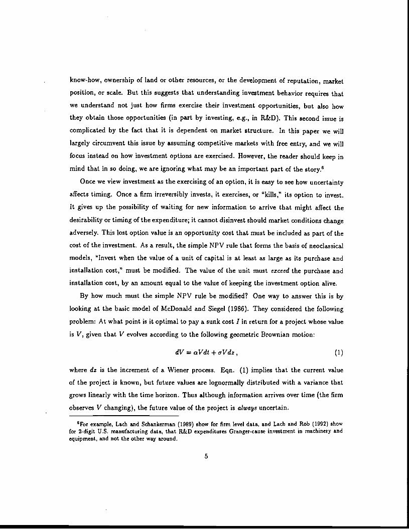
Figure 1: Dependence of V/I on o-.

0/3/Th7 < 0, this wedge is larger the greater is , i.e., the greater is the amount of uncertainty

over future values of V.

Characteristics of the Investment Decision.

It has been shown in several studies that the wedge between V and I can be quite

large for reasonable parameter values, so that investment rules that ignore the interaction of

uncertainty and irreversibility can be grossly in error. For example, if a =0 and p = 5 = .05,

V/I is 1.86 if o = .2, and is 3.27 if o- = .4. These numbers are conservative; in volatile

markets, the standard deviation of annual changes in a project's value can easily exceed 20

to 40 percent. Figure 1 shows V/1 as a function of o' for p = .04 and 6 = .02, .04, and .08.

Note that moderate changes in o (e.g., from 0.3 to 0.4) can lead to large changes in V/1,

particularly if 5 is small. Hence investment decisions can be highly sensitive to the extent of

volatility.

To see how the optimal investment rule depends on the other parameters, suppose the

firm is risk-neutral and p = r, where r is the risk-free interest rate. Let k = V/I = f3/(j3— 1)

12

10

0.0 0.1 0.2 0.3 0.4 0.5 0.6 0.7 0.8 0.9 D

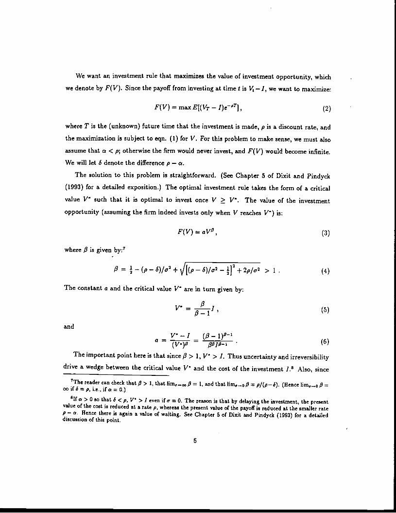
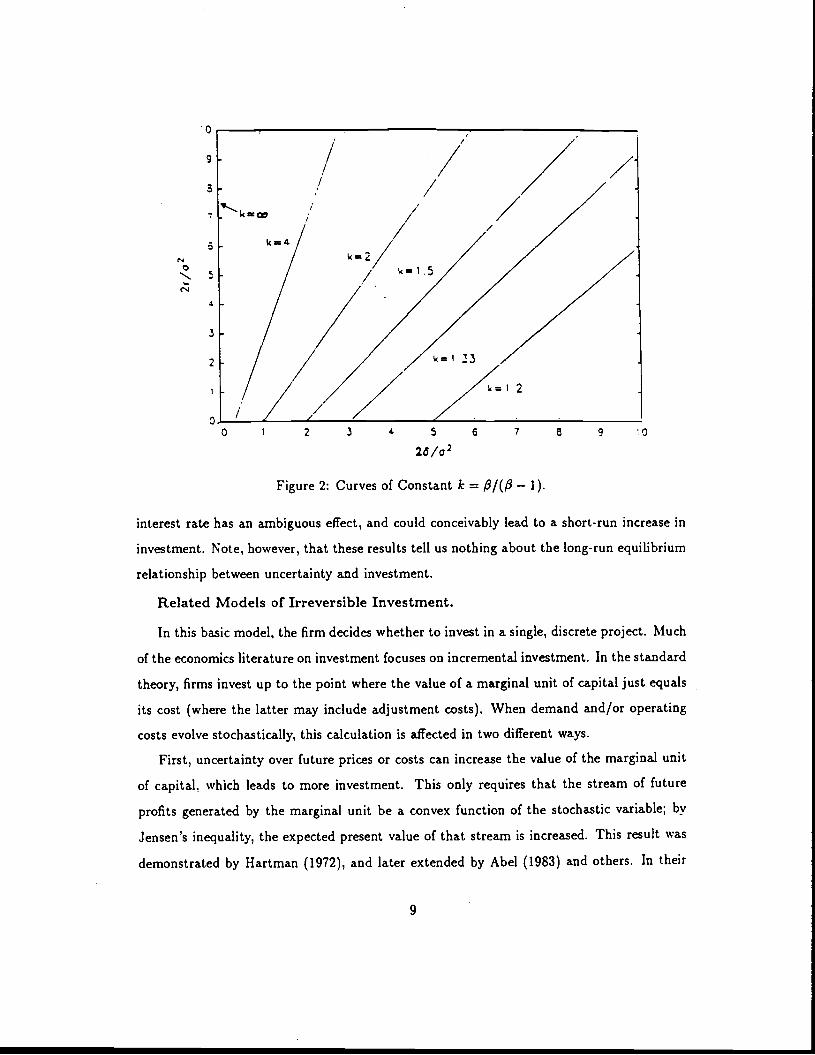
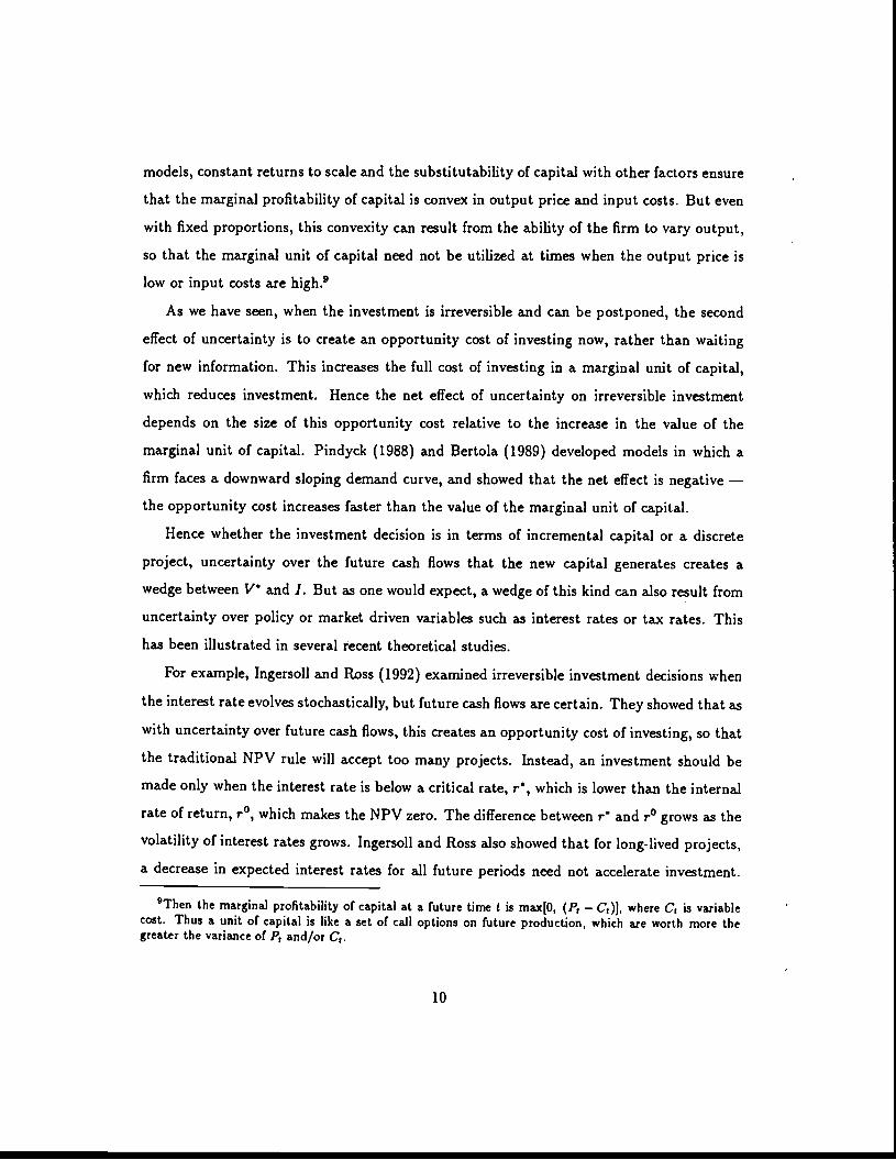
denote the multiple of I required to invest. Figure 2 shows iso-k lines plotted for different

values of 2r/u2 and 25/c2. We have scaled r and S by 2/c2 because k must satisfy:

2r kI'25'l k

c2) k—iAs the figure shows, the multiple k is smaller when 5 is large and larger when r is large.

As S becomes larger (holding everything else constant except for cr), the expected rate of

growth of V falls, and hence the expected appreciation in the value of the option to invest

and acquire V falls. In effect, it becomes costlier to wait rather than invest now.

On the other hand, when r is increased, F(V) increases, and so does V. Thereason is

that the present value of an investment expenditure I made at a future time T is IeT, but

the present value of the project that one receives in return for that expenditure is VeT.

Hence if S is fixed, an increase in r reduces the present value of the cost of the investment but

does not reduce its payoff. But note that while an increase in r raises the value ofa firm's

investment options, it also results in fewer of those options being exercised. Thus higher(real) interest rates can reduce investment, but for a different reason than in the standard

model. In the standard model, an increase in the interest rate reduces investment by raisingthe cost of capital; in this model it increases the value of the option to invest and henceincreases the opportunity cost of investing now.

In practice, however, an increase in r is likely to be accompanied by an increase in 5,because is unlikely to increase commensurately with r. The reason is that the expected

rate of capital gain on a project need not move with market interest rates. Hence it may bemore reasonable to assume that & remains fixed when interest rates change; then S = r —will move one-for-one with r. As Figure 2 shows, if r and S both increase by thesame amount,the multiple k will fall. Thus an increase in interest rates can stimulate investment in theshort run by reducing the incentive to wait.

In summary, this simple model shows how uncertainty and irreversibility create an op-

portunity cost of investing, which increases the expected return required for an investment.

That opportunity cost is an increasing function of the volatility of the project's value, sothat an increase in volatility can, in the short run, reduce investment. An increase in the real

8

N

Figure 2: Curves of Constant k = — 1).

interest rate has an ambiguous effect, and could conceivably lead to a short-run increase in

investment. Note, however, that these results tell us nothing about the long-run equilibrium

relationship between uncertainty and investment.

Related Models of Irreversible Investment.

In this basic model, the firm decides whether to invest in a single, discrete project. Much

of the economics literature on investment focuses on incremental investment. In the standard

theory, firms invest up to the point where the value of a marginal unit of capital just equals

its cost (where the latter may include adjustment costs). When demand and/or operating

costs evolve stochastically, this calculation is affected in two different ways.

First, uncertainty over future prices or costs can increase the value of the marginal unit

of capital. which leads to more investment. This only requires that the stream of future

profits generated by the marginal unit be a convex function of the stochastic variable; by

Jensen's inequality, the expected present value of that stream is increased. This result was

demonstrated by Hartman (1972), and later extended by Abel (1983) and others. In their

9

9

3

0 1 2 3 4 5 6 7 8 9 0

models, constant returns to scale and the substitutability of capital with other factors ensure

that the marginal profitability of capital is convex in output price and input costs. But even

with fixed proportions, this convexity can result from the ability of the firm to vary output,

so that the marginal unit of capital need not be utilized at times when the output price is

low or input costs are high.9

As we have seen, when the investment is irreversible and can be postponed, the second

effect of uncertainty is to create an opportunity cost of investing now, rather than waiting

for new information. This increases the full cost of investing in a marginal unit of capital,

which reduces investment. Hence the net effect of uncertainty on irreversible investment

depends on the size of this opportunity cost relative to the increase in the value of the

marginal unit of capital. Pindyck (1988) and Bertola (1989) developed models in which a

firm faces a downward sloping demand curve, and showed that the net effect is negative —

the opportunity cost increases faster than the value of the marginal unit of capital.

Hence whether the investment decision is in terms of incremental capital or a discrete

project, uncertainty over the future cash flows that the new capital generates creates a

wedge between V and I. But as one would expect, a wedge of this kind can also result from

uncertainty over policy or market driven variables such as interest rates or tax rates. This

has been illustrated in several recent theoretical studies.

For example, Ingersoll and Ross (1992) examined irreversible investment decisions when

the interest rate evolves stochastically, but future cash flows are certain. They showed that as

with uncertainty over future cash flows, this creates an opportunity cost of investing, so that

the traditional NPV rule will accept too many projects. Instead, an investment should be

made only when the interest rate is below a critical rate, r, which is lower than the internal

rate of return, r0, which makes the NPV zero. The difference between r and r0 grows as the

volatility of interest rates grows. Ingersoll and Ross also showed that for long-lived projects,

a decrease in expected interest rates for all future periods need not accelerate investment.

9Then the marginal profitability of capital at a future time t is max[O, (P — C)J, where C is variablecost. Thus a unit of capital is like a set of call options on future production, which are worth more thegreater the variance of P and/or C.

10

The reason is that such a change also lowers the cost of waiting, and thus can have an

ambiguous effect on investment. As another example, Rodrik (1989) examined the effects

of uncertainty over policy reforms designed to stimulate investment (e.g., a tax incentive).

He shows that if each year there is some probability that the policy will be reversed, the

resulting uncertainty can eliminate any stimulative effect that the policy would otherwise

have on investment.'0

Studies such as these suggest that levels of interest rates and tax rates may be of only

secondary importance as determinants of aggregate investment spending in the short run;

changes in interest rate volatility and policy instability may be more important. At issue

is whether there is empirical support for this view. We will turn to that question after

considering the effects of uncertainty in the context of a market equilibrium.

Industry Equilibrium.

So far we have discussed investment decisions by a single firm, taking price (or, for a

monopolist, demand) as exogenous. Our concern, however, is with investment at the industry

or aggregate level, so that price is endogenous. When studying the effects of uncertainty

on investment in the context of an industry equilibrium, two issues arise. First, we must

distinguish among the sources of uncertainty — aggregate (i.e., industry-wide) uncertainty

and idiosyncratic (i.e., firm-level) uncertainty can have very different effects on investment.

Second, the mechanism by which uncertainty affects investment is somewhat different at the

industry or aggregate level than it is for an isolated firm.

The fundamental determinants of investment are the distributions of future values of

the marginal profitability of capital — if these distributions are symmetric (and the firm is

risk-neutral), uncertainty will not affect investment. For a monopolist, irreversibility causes

the distributions to be asymmetric because the firm cannot disinvest in the future if negative

shocks arrive; hence the firm invests less today to reduce the frequency of bad outcomes in

the future (i.e., the frequency of situations in which the firm has more capital than desired).

'°Aizenman and Marion (1991) developed a similar model in which the tax rate can rise or fall, and showedthat this uncertainty can, in the short run, reduce irreversible investment in physical and human capital, andthereby suppress growth. They also show that various measures of policy uncertainty are in fact negativelycorrelated with real GDP growth in a cross section of 46 developing countries.

11

In a competitive industry with constant returns to scale, the distribution of the future

marginal profitability of capital for any particular firm is independent of that firm's current

investment. But this distribution is not independent of industry-wide investment.

This makes it important to distinguish between aggregate and idiosyncratic uncertainty.

To see this, consider idiosyncratic and aggregate shocks to productivity that are both sym-

metrically distributed. Although either type of shock can affect the expected future market

price and hence the expected marginal profitability of capital, the idiosyncratic shocks will

lead to a asymmetric probability distribution for the marginal profitability only insofar as

the marginal revenue product of capital is convex in the stochastic variable. Aggregate

shocks, however, will always lead to an asymmetric distribution. Although negative shocks

can reduce the market price, positive shocks will be accompanied by the entry of new firms

and/or expansion of existing firms, which will limit any increases in price. As a result, the

distribution of outcomes for individual firms is truncated; negative shocks to productivity

will reduce profits more than positive shocks will increase them, and irreversible investment

will be reduced accordingly.'1

In a recent paper, Caballero and Pindyck (1992) examined the effects of idiosyncratic

and aggregate uhcertainty using a simple model of a competitive market in which firms have

constant returns to scale and there is a sunk cost of entry. In their model the marginal

product of capital is linear in the stochastic state variables, thereby eliminating the positive

Jensen's inequality effect of uncertainty on the value of a marginal unit of capital thatarises from the endogenous response of variable factors to exogenous shocks. This lets them

focus on the way in which the effects of uncertainty are mediated through the equilibriumbehavior of all firms. They derive the critical rate of return required for investment, andshow how it is affected by aggregate (and not idiosyncratic) uncertainty, as well as other

parameters. They also show that the basic implications of the model are supported by 2-

digit U.S. manufacturing data. In the next section we show how a version of that modelcan

Pindyck (1993) and Chapters 8 and 9 of Dixit and Pindyck (1993) for more detailed discussionsof this point, and Dixit (1991), Leahy (1991), and Lippman and Rumelt (1985) for models of competitiveequilibrium with irreversible investment.

12

be used to study uncertainty and investment across countries.

3. Volatility, the Required Return, and Investment.In this section we summarize the model in Caballero and Pindyck (1992), slightly modified

to allow for differentiated products. We then review some implications of the model for

the behavior of the required rate of return and investment at the industry and aggregate

economy-wide levels.

Consider an economy with a large number N(t) of very small firms producing what may

be differentiated products, and let Q(i) be an index of aggregate consumption that reflects

tastes for diversity. We will represent Q(t) by the CES function:

N(t)Q(t) = j [A(t)]di ; 0 < p < 1, (7)

where A.(t) is the output of firm i. Hence the elasticity of substitution between any two

goods is 1/(1 —p)> 1.

Caballero and Pindyck decomposed the A1(i)'s into average (aggregate) and idiosyncratic

components, and allowed each component to follow a stochastic process. We also decompose

A(i), but we assume that the idiosyncratic component is constant:N(t)

A1(1) = A(t)a1, such that j a1di = N(t).

Thus A(t) is average productivity, so that Q(t) = A(i)N(t), and a is the productivity of unit.

i relative to the average. Note that N(t) can fluctuate over time, even though the a1's are

constant, as firms enter or exit. We will assume that aggregate productivity, A(t), follows

an exogenous stochastic process, and that the as's are randomly and uniformly distributed

across firms. At issue is whether each firm knows its own a, before entering, or only learns

it after entering; we address this below.

We take aggregate demand to be isoelastic:

P(t) = t)Q(i)/, (8)

where M(t) also follows an exogenous stochastic process representing aggregate demand

shocks. We also assume that there is an exogenous rate of depreciation or firm "failures," 6,

so that in the absence of entry, dN(t)/dt = —6N.

13

Assume for now that firms only learn their relative productivities a, after entry, so there

is no selective entry. Hence before entry, every firm expects to face the same price P. (Expost, some firms will produce more than others, so actual prices will vary.) To introduce

irreversibility, we assume that entry requires a sunk cost F. Then, free entry implies that:

F � E0 [j00P(t)A(t)e('*ö)t dt] , (9)

where r is the discount (interest) rate. The expectation E0 is over the distribution of the

future marginal profitability of capital, P(i)A4(i), and therefore accounts for the possible(irreversible) entry of new firms.

As long as we assume that firms cannot enter selectively, the results in Caballero and

Pindyck again apply. In this case, the marginal profitability of capital for a firmconsideringentry is the average value of output, which we denote by B(i):

B(t) P(i)A(t) =M(t)A(t)N(i) . (10)

We will assume that A(i) and M(t) follow uncorrelated geometric Brownian motions with

drift and volatility parameters c and a, and o,,, and Cm, respectively. Then B(t) will follow

a regulated geometric Brownian motion; entry will keep B(t) at or below a fixed boundary

U. When entry is not occurring, B(t) will follow a geometric Brownian motion, with a rateof drift:

,_ 12 77—1 1712— 0m — 2Cm + — + — ______

77 i 217

and with volatility:________________

= + ( 1)22As shown in Caballero and Pindyck (1992), the boundary U is given by:

U __ 2=1(r+5—fi—c6) , (11)

wher&2

_/3+fl2+2(r+o)o(12)

'2A solution will exist if the discount rate is large enough so that the value of a firm remains boundedeven if future entry is prohibited. This requires that 6 + — — > 0, so that ) > 1.

14

It is easy to show that E0 f°° Ue T+&)tdt > F. Because of irreversibility, there is an

opportunity cost of investing now rather than waiting; if firms could "uninvest" and recoup

the cost F, we would instead have the Marshallian result that E0 f'° Ue_(+E)tdt = F. It

can also be shown that 8(U/F)/Ooo > 0 and 8(U/F)/8/3 < 0, i.e., the opportunity cost

increases when the volatility of B(t) increases, and decreases when the rate at which B(i) is

expected to approach U increases. The reason for this first result should already be clear.

As for the second, an increase in (3 implies that B(t) will on average be closer to U, so that

there is a reduced risk of "bad" outcomes, and hence a smaller opportunity cost of making

a sunk cost investment.

Note that in this model, there is no investment until the expected "return" on a new

unit of capital, B(t)/F, reaches the critical level U/F, and then investment occurs so that

B(t)/F cannot rise above this level. This is a result of our assumption that there is no

selective entry, so that all firms face the same threshold for investment. It would be more

reasonable to assume that firms, which are heterogeneous, have at least some knowledge of

their relative productivities before they enter, so that they have different thresholds. Then

different firms will invest at different times, and for every firm the required threshold will

increase if the volatility of aggregate demand or productivity increases.

For example, suppose all potential entrants know their a's before entry. Then the free

entry condition (9) becomes:

F � a E0 [j°°P(t)A(t)e( dt] , (13)

Now the value of output for firm i is B,(t) = a,P(t)A(t) = a,B(t), and the firm will invest

when B, reaches a threshold U,. However, in this case the value of the firm will depend

not only on B(t), but also on the number of firms N(t) currently producing. This adds

another state variable to the problem, so that (given some distribution for the a,'s) finding

(.J requires the solution of a partial differential equation for the value function.

Empirical Implications.

It is important to be clear about what this model and others like it do and do not tell

us about uncertainty and its effects on investment. First, note that these models do not

15

describe investment per se, but rather the critical threshold required to trigger investment.

In the model of an industry equilibrium discussed above, the threshold is U; in thesimplemodel of investment in a single project reviewed in the preceding section, the threshold was

a critical project value, V'. In both cases the predictions of the models were with respect

to the dependence of the threshold on volatility and other parameters. The models tellus

that if volatility increases, the threshold increases.13 Only to the extent that we can also

describe (or make assumptions about) the distribution across firms of the values ofpotentialprojects, or of the marginal profitability of capital, can we also derive a structural model

that relates volatility to actual investment.

Even without going this far, we can draw inferences from these models with regard tothe ways in which investment should respond in the short run to changes in volatility and

other parameters. For example, a one-time increase in volatility should reduceinvestment

at least temporarily, as project values that were above or close to what was a lower critical

threshold are now below a higher one. Second, we saw in our equilibrium model above that

an increase in the drift, /3, lowers the critical threshold, and hence should be accompaniedby an increase in investment.'4 Hence increases in the volatility of the marginal profitabilityof capital, or decreases in its average growth rate (when it is below the boundary U), should

lead to at least a temporary decrease in investment. In the next section we will discuss thisin more detail in the context of our empirical tests.

Unfortunately, there is very little that can be said about the effects of uncertainty on thelong-run equilibrium values of investment, the investment-to-output ratio, or the capital-output ratio. To see this, note that although we know that an increase in volatility raisesthe required return needed to trigger investment,we do not know what it will do the average

'3Thia is not exactly correct, in that we have assumed in these models that volatility is constant. Ifvolatility can change, predictably or unpredictably, then in principle the process by which it changes shouldbe part of the model. However, models of financial option valuation in which volatility follows a stochasticprocess suggest that adding this complication would not change our results substantially. For examples ofoption valuation models with stochastic volatility, see Hull and White (1987), Scott (1987), and Wiggins(1987).

'4Remember that B(t), the marginal profitability of capital, follows a regulated and therefore stationaryprocess. The parameter is the drift of B(t) when it is below the threshold (i.e., upper boundary), U.

16

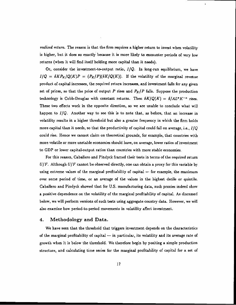
realized return. The reason is that the firm requires a higher return to invest when volatility

is higher, but it does so exactly because it is more likely to encounter periods of very low

returns (when it will find itself holding more capital than it needs).

Or, consider the investment-to-output ratio, I/Q. In long-run equilibrium, we have

I/Q = I5KPK/Q(K)P = (PK/P)(6K/Q(K)). If the volatility of the ma.rgina.l revenue

product of capital increases, the required return increases, and investment falls for any given

set of prices, so that the price of output P rises and PK/P falls. Suppose the production

technology is Cobb-Douglas with constant returns. Then LK/Q(K) = ö/AL°K° rises.

These two effects work in the opposite direction, so we are unable to conclude what will

happen to I/Q. Another way to see this is to note that, as before, that an increase in

volatility results in a higher threshold but also a greater frequency in which the firm holds

more capital than it needs, so that the productivity of capital could fall on average, i.e., I/Q

could rise. Hence we cannot claim on theoretical grounds, for example, that countries with

more volatile or more unstable economies should have, on average, lower ratios of investment

to GDP or lower capital-output ratios than countries with more stable economies.

For this reason, Caballero and Pindyck framed their tests in terms of the required return

U/F. Although U/F cannot be observed directly, one can obtain a proxy for this variable by

using extreme values of the marginal profitability of capital — for example, the maximum

over some period of time, or an average of the values in the highest decile or quintile.

Caballero and Pindyck showed that for U.S. manufacturing data, such proxies indeed show

a positive dependence on the volatility of the marginal profitability of capital. As discussed

below, we will perform versions of such tests using aggregate country data. However, we will

also examine how period-to-period movements in volatility affect investment.

4. Methodology and Data.We have seen that the threshold that triggers investment depends on the characteristics

of the marginal profitability of capital — in particular, its volatility and its average rate of

growth when it is below the threshold. We therefore begin by positing a simple production

structure, and calculating time series for the marginal profitability of capital for a set of

17

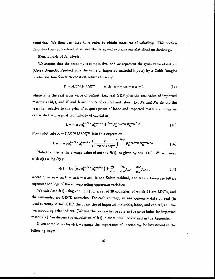
countries. We then use these time series to obtain measures of volatility. This section

describes these procedures, discusses the data, and explains our statistical methodology.

Framework of Analysis.

We assume that the economy is competitive, and we represent the gross value of output

(Gross Domestic Product plus the value of imported material inputs) by a Cobb-Douglas

production function with constant returns to scale:

Y = AKKLOLMJCIM with aj + aL + M = 1, (14)

where Y is the real gross value of output, i.e., real GDP plus the real value of imported

materials (M,), and K and L are inputs of capital and labor. Let PL and PM denote the

real (i.e., relative to the price of output) prices of labor and imported materials. Then we

can write the marginal profitability of capital as:

ilK (15)

Now substitute A = Y/KaKLOLMIQM into this expression:

= aK0LL 1M/0K (KoKLM;M)paL/aKp;OM/Ox (16)

Note that 11K is the average value of output B(i), as given by eqn. (10). We will work

with &(t) = log fl(t):

b(i) = log + -- — — PM,i, (17)K K aKwhere a1 = — aKkj — — aMin1 is the Solow residual, and where lowercase letters

represent the logs of the corresponding uppercase variables.

We calculate b(i) using eqn. (17) for a set of 30 countries, of which 14 are LDC's, and

the remainder are OECD countries. For each country, we use aggregate data on real (in

local currency terms) GDP, the quantities of imported materials, labor, and capital, and the

corresponding price indices. (We use the real exchange rate as the price index for imported

materials.) We discuss the calculation of b(s) in more detail below and in the Appendix.

Given these series for b(i), we gauge the importance of uncertainty for investment in the

following ways:

18

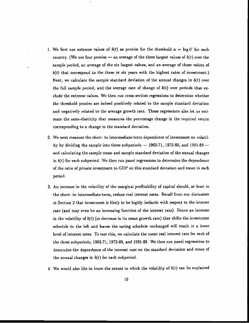
1. We first use extreme values of 6(1) as proxies for the threshold u = logU for each

country. (We use four proxies — an average of the three largest values of b(t) over the

sample period, an average of the six largest values, and an average of those values of

6(1) that correspond to the three or six years with the highest rates of investment.)

Next, we calculate the sample standard deviation of the annual changes in b(t) over

the full sample period, and the average rate of change of 6(t) over periods that ex-

clude the extreme values. We then run cross-section regressions to determine whether

the threshold proxies are indeed positively related to the sample standard deviation

and negatively related to the average growth rate. These regressions also let us esti-

mate the semi-elasticity that measures the percentage change in the required return

corresponding to a change in the standard deviation.

2. We next measure the short- to intermediate-term dependence of investment on volatil-

ity by dividing the sample into three subperiods — 1962-71, 1972-80, and 1981-89 —

and calculating the sample mean and sample standard deviation of the annual changes

in 6(t) for each subperiod. We then run panel regressions to determine the dependence

of the ratio of private investment to GDP on this standard deviation and mean in each

period.

3. An increase in the volatility of the marginal profitability of capital should, at least in

the short- to intermediate-term, reduce real interest rates. Recall from our discussion

in Section 2 that investment is likely to be highly inelastic with respect to the interest

rate (and may even be an increasing function of the interest rate). Hence an increase

in the volatility of b(t) (or decrease in its mean growth rate) that shifts the investment

schedule to the left and leaves the saving schedule unchanged will result in a lower

level of interest rates. To test this, we calculate the mean real interest rate for each of

the three subperiods, 1962-71, 1972-80, and 1981-89. We then run panel regressions to

determine the dependence of the interest rate on the standard deviation and mean of

the annual changes in 6(t) for each subperiod.

4. We would also like to know the extent to which the volatility of 6(t) can be explained

19

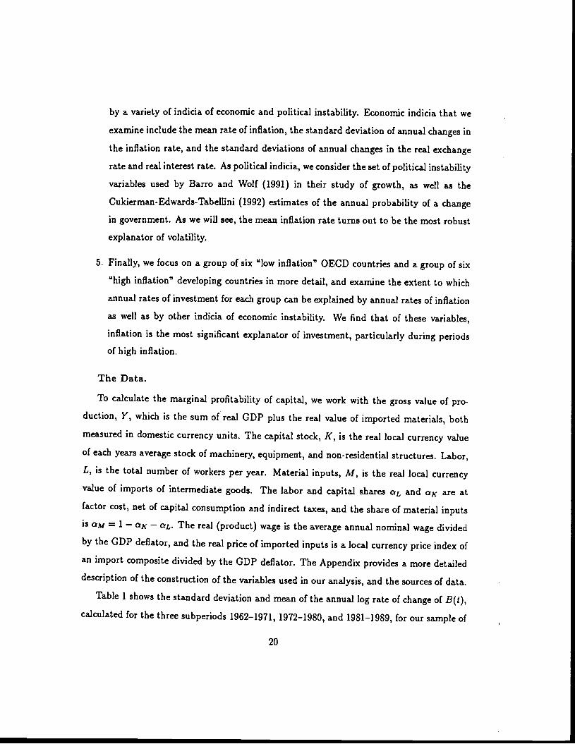
by a variety of indicia of economic and political instability. Economic indicia that we

examine include the mean rate of inflation, the standard deviation of annual changes in

the inflation rate, and the standard deviations of annual changes in the real exchange

rate and real interest rate. As political indicia, we consider the set of political instability

variables used by Barro and Wolf (1991) in their study of growth, as well as the

Cukierman-Edwards-Tabellini (1992) estimates of the annual probability of a change

in government. As we will see, the mean inflation rate turns out to be the most robust

explanator of volatility.

5. Finally, we focus on a group of six "low inflation" OECD countries and a group of six

"high inflation" developing countries in more detail, and examine the extent to which

annual rates of investment for each group can be explained by annual rates of inflation

as well as by other indicia of economic instability. We find that of these variables,

inflation is the most significant explanator of investment, particularly during periodsof high inflation.

The Data.

To calculate the marginal profitability of capital, we work with the gross value of pro-

duction, Y, which is the sum of real GDP plus the real value of imported materials, both

measured in domestic currency units. The capital stock, K, is the real localcurrency value

of each years average stock of machinery, equipment, and non-residential structures. Labor,

L, is the total number of workers per year. Material inputs, M, is the real local currency

value of imports of intermediate goods. The labor and capital shares and o,t- are at

factor cost, net of capital consumption and indirect taxes, and the share of materialinputsis cM = 1 — cxx — cxL. The real (product) wage is the average annual nominal wage divided

by the GDP deflator, and the real price of imported inputs is a localcurrency price index of

an import composite divided by the GDP deflator. The Appendix provides a more detailed

description of the construction of the variables used in our analysis, and thesources of data.

Table 1 shows the standard deviation and mean of the annual log rate ofchange of B(i),

calculated for the three subperiods 1962—1971, 1972—1980, and 1981—1989, forour sample of

20

30 countries. Also shown is the average value of the ratio of private investment-to-GDP for

each interval of time. Our regressions will use these subperiod averages, as well as averages

for the entire sample period. Note that the standard deviations and means for the Philippines

are about an order of magnitude larger than those for the other countries. This is due to very

large annual fluctuations (up to 50 percent) in the data for the real wage in the Philippines.

We find the wage data difficult to believe, so we omit the Philippines from our sample in all

of the work that follows.

5. Cross-Section Evidence.In this section we use our cross-section of countries to examine the dependence of in-

vestment and its determinants on the volatility of the marginal profitability of capital. \Ve

first work with proxies for the threshold (or required return), and then look directly at the

dependence of investment on volatility using averages for our three subperiods. We also ex-

amine the dependence of interest rates on volatility, again using averages for the subperiods.

In each case we will focus on differences between LDC's and OECD countries.

Volatility and the Required Return.

Changes in the volatility of the marginal profitability of capital affect investment by

affecting the threshold at which firms invest. At the aggregate level, firms with different

productivities will hit their thresholds at different times, so there will always be some invest-

ment taking place. When the marginal profitability of capital is high relative to its average

value, more firms will be hitting their thresholds and aggregate investment should be higher.

Hence although we cannot observe the threshold directly, we can use extreme values of b(t)

as a proxy.

As in Caballero and Pindyck (1992), we examine several different variables. First, we

compute the average of the top decile (three observations) of the 28 annual values of b(s)

for each country, which we denote by DBDEC, and the average of the top quintile (six

observations), which we denote by DBQUINT. In both cases we calculate these values

relative to the country mean of 6(i). We average over several extreme values rather than

using the maximum value because b(t) may rise above the threshold u temporarily if there

21

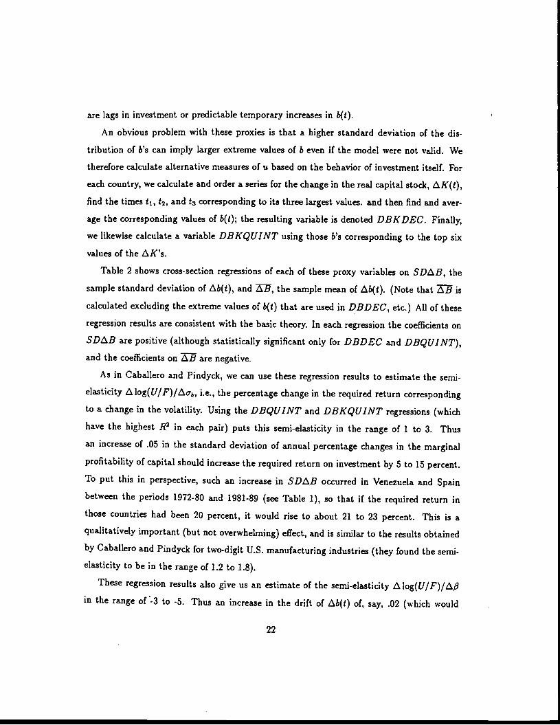
are lags in investment or predictable temporary increases in b(L).

An obvious problem with these proxies is that a higher standard deviation of the dis-

tribution of b's can imply larger extreme values of b even if the model were not valid. We

therefore calculate alternative measures of u based on the behavior of investment itself. For

each country, we calculate and order a series for the change in the real capital stock, EK(i),

find the times t1, t2, and i3 corresponding to its three largest values, and then find and aver-

age the corresponding values of b(t); the resulting variable is denoted DBKDEC. Finally,

we likewise calculate a variable DBK QUINT using those b's corresponding to the top six

values of the EK's.

Table 2 shows cross-section regressions of each of these proxy variables on SDtB, the

sample standard deviation of b(t), and , the sample mean of b(t). (Note that is

calculated excluding the extreme values of b(i) that are used in DBDEC, etc.) All of these

regression results are consistent with the basic theory. In each regression the coefficients on

SDLB are positive (although statistically significant only for DBDEC and DR QUINT),

and the coefficients on are negative.

As in Caballero and Pindyck, we can use these regression results to estimate the semi-

elasticity i log(U/F)/zo-, i.e., the percentage change in the required return corresponding

to a change in the volatility. Using the DBQUINT and DBK QUINT regressions (which

have the highest R2 in each pair) puts this semi-elasticity in the range of 1 to 3. Thus

an increase of .05 in the standard deviation of annual percentage changes in the marginal

profitability of capital should increase the required return on investment by 5 to 15 percent.

To put this in perspective, such an increase in SDtB occurred in Venezuela and Spain

between the periods 1972-80 and 1981-89 (see Table 1), so that if the required return in

those countries had been 20 percent, it would rise to about 21 to 23 percent. This is a

qualitatively important (but not overwhelming) effect, and is similar to the results obtained

by Caballero and Pindyck for two-digit U.S. manufacturing industries (they found the semi-

elasticity to be in the range of 1.2 to 1.8).

These regression results also give us an estimate of the semi-elasticity iIog(U/F)/i$in the range of'-3 to -5. Thus an increase in the drift of b(t) of, say, .02 (which would

22

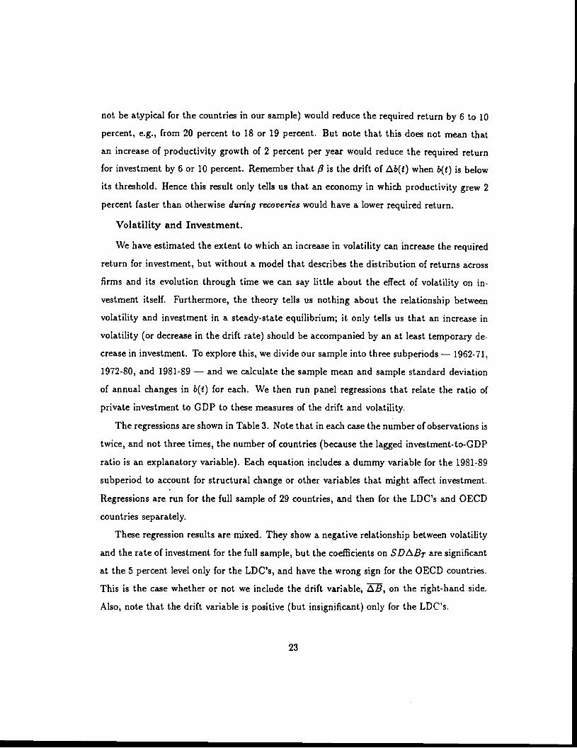
not be atypical for the countries in our sample) would reduce the required return by 6 to 10

percent, e.g., from 20 percent to 18 or 19 percent. But note that this does not mean that

an increase of productivity growth of 2 percent per year would reduce the required return

for investment by 6 or 10 percent. Remember that is the drift of tb(i) when b(t) is below

its threshold. Hence this result only tells us that an economy in which productivity grew 2

percent faster than otherwise during recoveries would have a lower required return.

Volatility and Investment.

We have estimated the extent to which an increase in volatility can increase the required

return for investment, but without a model that describes the distribution of returns across

firms and its evolution through time we can say little about the effect of volatility on in-

vestment itself. Furthermore, the theory tells us nothing about the relationship between

volatility and investment in a steady-state equilibrium; it only tells us that an increase in

volatility (or decrease in the drift rate) should be accompanied by an at least temporary de-

crease in investment. To explore this, we divide our sample into three subperiods —1962-71,

1972-80, and 1981-89 — and we calculate the sample mean and sample standard deviation

of annual changes in b(i) for each. We then run panel regressions that relate the ratio of

private investment to GDP to these measures of the drift and volatility.

The regressions are shown in Table 3. Note that in each case the number of observations is

twice, and not three times, the number of countries (because the lagged investment-to-GDP

ratio is an explanatory variable). Each equation includes a dummy variable for the 1981-89

subperiod to account for structural change or other variables that might affect investment.

Regressions are run for the full sample of 29 countries, and then for the LDC's and OECD

countries separately.

These regression results are mixed. They show a negative relationship between volatility

and the rate of investment for the full sample, but the coefficients on SDLBT are significant

at the 5 percent level only for the LDC's, and have the wrong sign for the OECD countries.

This is the case whether or not we include the drift variable, , on the right-hand side.

Also, note that the drift variable is positive (but insignificant) only for the LDC's.

23

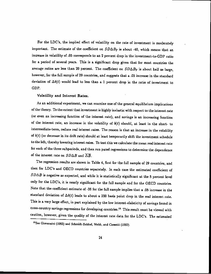
For the LDC's, the implied effect of volatility on the rate of investment is moderately

important. The estimate of the coefficient on SDtiBr is about -40, which means that an

increase in volatility of .05 corresponds to an 2 percent drop in the investment-to-GDP ratio

for a period of several years. This is a significant drop given that for most countries the

average ratios are less than 20 percent. The coefficient on SDBT is about half as large,

however, for the full sample of 29 countries, and suggests that a .05 increase in the standard

deviation of b(t) would lead to less than a 1 percent drop in the ratio of investment to

GD P.

Volatility and Interest Rates.

As an additional experiment, we can examine one of the general equilibrium implications

of the theory. To the extent that investment is highly inelastic with respect to the interest rate

(or even an increasing function of the interest rate), and savings is an increasing function

of the interest rate, an increase in the volatility of b(t) should, at least in the short- to

intermediate-term, reduce real interest rates. The reason is that an increase in the volatility

of b(t) (or decrease in its drift rate) should at least temporarily shift the investment schedule

to the left, thereby lowering interest rates. To test this we calculate the mean real interestratefor each of the three subperiods, and then run panel regressions to determine thedependenceof the interest rate on SDB and .

The regression results are shown in Table 4, first for the full sample of 29 countries, and

then for LDC's and OECD countries separately. In each case the estimated coefficient ofSDi1B is negative as expected, and while it is statistically significant at the 5 percent level

only for the LDC's, it is nearly significant for the full sample and for the OECD countries.

Note that the coefficient estimate of -38 for the full sample implies that a .05 increase in the

standard deviation of Ab(t) leads to about a 200 basis point drop in the real interest rate.

This is a very large effect, in part explained by the low interest-elaisticity of savings found in

cross-country savings regressions for developing countries.'5 This result must be viewed with

caution, however, given the quality of the interest rate data for the LDC's. The estimated

'5See Giovannirij (1983) and Schmidt-Hebbel, Webb, and Corsetti (1992).

24

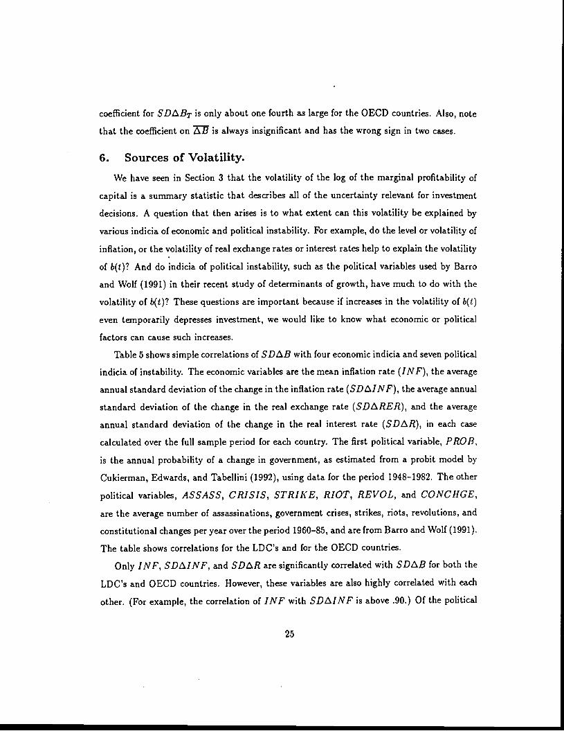
coefficient for SDt.BT is only about one fourth as large for the OECD countries. Also, note

that the coefficient on is always insignificant and has the wrong sign in two cases.

6. Sources of Volatility.

We have seen in Section 3 that the volatility of the log of the marginal profitability of

capital is a summary statistic that describes all of the uncertainty relevant for investment

decisions. A question that then arises is to what extent can this volatility be explained by

various indicia of economic and political instability. For example, do the level or volatility of

inflation, or the volatility of real exchange rates or interest rates help to explain the volatility

of b(t)? And do indicia of political instability, such as the political variables used by Barro

and Wolf (1991) in their recent study of determinants of growth, have much to do with the

volatility of b(i)? These questions are important because if increases in the volatility of b(1)

even temporarily depresses investment, we would like to know what economic or political

factors can cause such increases.

Table 5 shows simple correlations of SDB with four economic indicia and seven political

indicia of instability. The economic variables are the mean inflation rate (IN F), the average

annual standard deviation of the change in the inflation rate (SDiINF), the average annual

standard deviation of the change in the real exchange rate (SDiRER), and the average

annual standard deviation of the change in the real interest rate (SDR), in each case

calculated over the full sample period for each country. The first political variable, PROB,

is the annual probability of a change in government, as estimated from a probit model by

Cukierman, Edwards, and Tabellini (1992), using data for the period 1948—1982. The other

political variables, ASSASS, CRISIS, STRIKE, RIOT, REVOL, and CONCHGE,

are the average number of assassinations, government crises, strikes, riots, revolutions, and

constitutional changes per year over the period 1960—85, and are from Barro and Wolf (1991).

The table shows correlations for the LDC's and for the OECD countries.

Only INF, SDLINF, and SDLIR are significantly correlated with SDtB for both the

LDC's and OECD countries. However, these variables are also highly correlated with each

other. (For example, the correlation of INF with SDLtINF is above .90.) Of the political

25

variables, only ASSASS, STRIKE, and RIOT are significantly correlated with SDB,and then only for the LDC's.

We ran a large set of cross-section regressions in order to explore the ability of these

economic and political variables to "explain" the volatility of 6(i). Table 6 shows only asmall subset of these regressions, but the results are representative of our overall findings.Most important, the mean inflation rate is the only variable that is consistentlysignificant as

an explanator of SDLiB. Although SDINF and SDEIR are individually correlated with

SDB, they are always insignificant when combined with INF in a regression. STRIKE

is also significant in these regressions, but only for the LDC's. As longas INF is also in the

regression, all of the other political variables are either insignificant and/or have the wrongsign. This is true for the LDC's, the OECD countries, or when the regressions arerun overthe full sample.

This suggests that strikes, riots, revolutions, and other forms ofpolitical turmoil and

uncertainty (as measured by these indicia) may have little to do with uncertainty over thereturn on capital, and hence with investment. It may mean that as long as a governmentcan control inflation — an indicator of overall economic stability, and from which exchangerate and interest rate stability tend to follow — it can limit the uncertainty that mattersfor investment. These results also raise doubts regarding recent results in the literature that

relate indicia of political instability to growth. On the other hand, regressions of the sortshown in Table 6 have serious limitations. Aside from the very limited sample of countries,the most important limitation is our assumption that the relevant stochastic state variablesfollow Brownian motions, so that 6(1) follows a controlled Brownian motion. This eliminates"peso problems" as a source of uncertainty.

If we take these results at face value, they suggest that controlling inflation should beone of the most important intermediate objectives of policy. We explore this in more detailin the next section.

7. Time Series Evidence.

The cross-country evidence presented above suggests that inflation may be one of the

26

best indicia of economic instability, and is associated with lower rates of capital formation.

This seems to be particularly true at very high levels of inflation. In this section we explore

the relationship between inflation and investment in more detail by examining a group of

six OECD countries that have had relatively low inflation, and a group of high inflation

countries, predominantly in Latin America. Our objective is to examine the robustness of

the relationship between inflation and investment across countries with very different levels

of inflation, and to explore possible nonlinearities in this relationship within each country

group.

To do this, we study the relationship between year-to-year variation in different indicators

of economic instability and the ratio of investment to GDP. This is important, because our

use of nine-year averages in Section 5 may have concealed higher-frequency information.

In this section we report on panel regressions that utilize annual data relating the ratio of

investment to GDP (total and private) directly to three indicia of economic instability — the

level and variability of inflation, and the variability of the real exchange rate. (Unfortunately

annual data are not available for indicia of social and political instability.) This allows us

to capture possible effects of economic instability on investment that may occur though

channels other than the volatility of the marginal profitability of capital.'6

Of particular concern to us is inflation, which can affect investment in several ways:

(i) High and volatile inflation may indicate an inability of the government to control the

economy (see Fischer (1993)). As a consequence, government policies will be perceived by

investors as unsustainable and hence risky, leading them to defer investing. (ii) High and

volatile inflation is associated with greater volatility in the marginal profitability of capital,

and with volatile relative prices (see Fischer and Modigliani (1978) and Fischer (1986)).

(iii) Inflation amounts to a tax on real monetary balances. Hence if money and capital are

complementary — through the production function or through cash-in-advance constraints

— inflation and investment will be negatively correlated.'7

16Fischer (1986, 1991, 1993) discusses several channels through which inflation may affect growth andcapital formation.

'7Fischer (1993) and Kormendi and Meguire (1985) have found such a negative correlation.

27

Low Inflation OECD Countries.

We first estimate a fixed effects panel regression for the ratio of total investment to GD?

for France, Germany, Japan, the Netherlands, the United Kingdom and the United States,

using annual data covering the period 1960 to 1990. In this model the investment-to-GD?

ratio is a function of variables such as the rate of inflation, the standard deviation of annual

changes in the inflation rate, and the standard deviation of annual changes in the real ex-

change rate, as well as the lagged rate of real GD? growth and the lagged investment-to-GD?

ratio. In the estimation, the White procedure was used to correct for heteroscedastjc errors

and the H-test did not reject the null hypothesis of absence of first-order serial correlation.

Each variable is measured as a deviation from its corresponding country mean, so that themodel can be written as:

(J/GDP)jg = a1JNF1,, + a2SDINF1 + a3SDRER,,, + a4GRTH_1 + as(I/GDP)_1 +

(18)where (I/GDP),, is the ratio of investment to GD? in country i in year 1, INF is the meaninflation rate for the year, SDINF is the sample standard deviation of eachyear's monthlyobservations of inflation, SDRER is the sample standard deviation of the real exchangerate, and GRTH is the rate of growth of real GD?.

Selected results of estimating this model for total investment are shown in Table 7.(The results are similar for private investment.) The economic volatility variables INF,SDJNF, and SDRER are highly correlated with each other, but when all threeare included

in the regression, only the coefficient of INF in negative and significant. INF is alsohighly significant in any pairwise combination with SDJNF and SDRER, but SDRERis significant only by itself or in combination with SDJNF. These results suggest that ofthe three indicia of economic volatility, the level of inflation is the most robust explanator

of investment, but the volatility of relative prices — proxied by the volatility of the realexchange rate — has an independent contribution in explaining investment.

To further explore the relationship between inflation and investment for this group ofcountries, we show in Figure 3 the average values for both variables for the subperiods

28

1960-1973 and 1974-1990. Note that the negative relationship between inflation and the

investment-to-GDP ratio is strongest for average rates of inflation above 5 percent per year;

below that level the relationship is blurred. As the scatter diagram shows, most instances of

average annual inflation rates over the 5 percent threshold belong to the period 1974-90, when

inflation accelerated and capital formation declined in the OECD largely as a consequence

of the two oil price shocks and the subsequent adjustment process.

High Inflation Countries (Latin America and Israel).

Similar panel regression were estimated for Argentina, Bolivia, Bra.zil, Chile, Israel, and

Mexico, also using annual data for the period 1960-1990. Table 8 shows selected regressions

results, first for total investment and then for private.

Note that inflation always appears with a negative coefficient, but is statistically signifi-

cant only for the total investment regressions. The standard deviation of inflation is always

insignificant (and has a coefficient of correlation with the level of inflation of .89 in this

sample), and the standard deviation of the real exchange rate is negative and significant

in two of the three total investment equations. These results are again consistent with the

view that inflation, and to a lesser extent the variability of relative prices, are what matter

most for investment. Finally, when the ratio of public investment to GDP is included in the

equations for private investment, it is always negative and significant, suggesting a crowding

out effect.

To explore potential nonlinearities in the relation between inflation and investment, and

also to relate the duration of the spells of high inflation to their impact, it is useful to

classify different inflationary experiences in terms of their intensity. One classification (more

appropriate for "chronic" high inflation countries) was proposed by Dornbusch and Fischer

(1991): (i) moderate inflation refers to rates of price increase between 15 and 30 percent per

year for at least three consecutive years; (ii) high inflation refers to rates between 30 and

100 percent per year; (iii) extreme inflation refers to rates between 100 and 1,000 percent

per year; and (iv) hyperinflation refers to rates above 1,000 percent per year.'8

'8The norm of inflation clearly depends on the region or country. For several OECD economies, rates ofinflation in excess of 10 percent per year would be considered as intolerable or "extreme".

29

Table 9 summarizes the experiences of inflation and their aftermath for several countries.

It shows that the slide from "low" to "moderate" inflation has no significant effect on capital

formation. On the contrary, in some cases, like Mexico and Korea in the mid to late 1970s,

the slide from low inflation to moderate inflation came along with an increase in (mostly

public) investment rates.'9

On the other hand, Table 9 shows that in countries in which inflation went from low

to high two-digit levels and then to three digits, investment was more severely affected.

For example, in Mexico, Brazil, and Israel, investment declined by 5 percentage points of

GDP (or more) in the 1980s (a period of severe acceleration of inflation in these countries)

compared to the average levels of the 1960s and 1970s.

A more extreme case of protracted instability is Argentina. This country had an average

annual inflation rate around 260 percent for 14 years — between 1975 and 1988 — before

drifting to hyperinflation in 1989-90. This is a case of extremely prolonged inflation and at a

very high level. No wonder, then, that capital formation collapsed in Argentina in the 1980s;

the share of investment in GDP declined by more than 10 percentage points in the 1980s

from its average of the 1960s and 1970s. Another extreme case is Bolivia, which experienced

hyperinflation in 198485.20

Regarding the duration of the spells of inflation the data show that the higher the rate

of inflation, the shorter the duration of the inflationary episode. Low and moderate inflation

(below 30 percent per year) tend to be relatively stable, high inflation (between 30 and 100

percent) less so, three-digit infiations often last between 2 to 5 years, and hyperinflation may

last from 6 months to 18 months.

Figures 4 and 5 show the relationship between inflation and the ratio of investment (total

and private) to CDP for Argentina, Bolivia, Brazil, Chile, Israel and Mexico, using decade

averages for the 1960s, 1970s and 1980s. These figures show a negative relationship between

'9See Lustig (1992) and Collins and Park (1989). In fact, in the short term, inflation and investment maymove in the same direction following an increase in public investment or other exogenous demand shock.

20The share of total investment in GDP in Bolivia was only 9 percent in the period 1983-90, down from 23percent in the pre-inflation period. The period 1983—90 includes both the hyperinflation and its subsequentstabilization.

30

the average rate of inflation and the average investment-to-GDP ratio when annualinflation

is over 50 percent (particularly during the 1970 and 1980s). However, when the averageannual inflation rate is less than 50 percent (e.g. in the 1960s), the relationship between

inflation and investment is much less clear. This suggests that the relationship between

inflation and investment is highly nonlinear.

Stabilizations and the Response of Investment.

Stabilizing inflation is a precondition for a resumption of investment in aneconomy that

has undergone a period of high price instability. However, accumulated evidence shows that

the resumption of investment and growth after the implementation of a stabilization pro-

gram is a slow process. There are several reasons for this: (i) restrictive monetary policies

push up real interest rates, thus depressing investment and output growth; (ii) there is a

potential credibility problem in the aftermath of stabilization that makes investors reluctant

to commit resources given doubts as to whether the stabilizationprogram will succeed. This

tends to delay the recovery of investment in the aftermath of stabilization; (iii)governments

tend to cut public investment during the course of fiscal adjustment, and if public invest-

ment, particularly in infrastructure, telecommunications and the like, is complementary with

private investment, this will contribute to a decline in aggregate capital accumulation; (iv)

If the stabilization program takes place in a context of reduced foreign financing (e.g. Latin

America in the 1980s), the resumption of investment in the aftermath of stabilization will

be more elusive. (See Sachs (1989) and Serven and Solimano (1992, 1993).)

Table 10 summarizes four stabilization programs carried out in the 1970s and 1980s:

Chile (1975), Israel (1985), Bolivia (1985), and Mexico (late 1987).21 In three of the four

cases, the investment share remained below its pre-inflation during the first five years after

the stabilization program was launched, suggesting that the resumption of investment (and

growth) after the implementation of a stabilization program is a slow process.22

21For recent studies of these stabilization programs see Cobo and Solimano (1991) for Chile, Bruno andMeridor (1991) for Israel, Morales (1991) for Bolivia, and Ortiz (1991) for Mexico. Chile and Bolivia arecases of orthodox stabilization (money based), and Israel and Mexico are cases of heterodox stabilization(multiple-anchor); see Bruno et. al. (1991) and Kiguel and Liviatan (1992).

22For additional evidence on this for a larger group of countries, see Dornbusch (1991), Corden (1991),

31

Also, there seems to be no correlation between the speed of disinflation and the speed of

investment recovery. Bolivia ended its hyperinflation of 1985 very quickly, while investment

remained depressed for many years thereafter. In contrast, disinflation in Chile after 1975

was slow and the immediate investment response to the stabilization plan was fast.23 As for

the effect of program characteristics on the performance of investment after stabilization,

the evidence shows no clear differences in the behavior of investment between orthodox

(money-based) and heterodox (multiple-anchor-based) stabilization programs.

In summary, the country evidence shows that the restoration of stability after a period

of high inflation and uncertainty is likely to be accompanied by depressed capital formation,

as investors require time to be convinced that the uncertainty is indeed reduced and that

stability will be consolidated.

8. Conclusions.

We have outlined some of the empirical implications of the recent theoretical literature

on irreversible investment and the value of waiting, and then examined its relevance for

aggregate investment in a set of industrialized and developing countries. We have shown

that if the exogenous stochastic state variables follow Brownian motions, uncertainty can be

summarized by the volatility of the marginal profitability of capital, which will itself follow a

controlled Brownian motion. An increase in this volatility will increase the critical required

return for investment, and hence should reduce investment spending — in the short run.

Unfortunately, we can say little about the effect of such an increase in volatility on the long-

run steady-state level of investment, investment-to-output ratio, or other such measures.

This does not mean, however, that volatility is not an important determinant of invest-

ment spending. Given the lags involved in planning and implementing large-scale invest-

ment programs, and given that the real and perceived riskiness of investing can change over

decades, the "short run" can easily be ten or twenty years.

We therefore conducted our empirical tests by examining the relationship between volatil-

Solimano (1992a).

"See Solimano (1992b).

32

ity and investment across decades for a set of countries. We found that the relationship is

negative but moderate in size, and is of greater magnitude for developing countries. We also

tried to relate the volatility of the marginal profitability of capital to indicia of economic

instability — such as inflation and its volatility —and to indicia of political instability. Only

inflation is at all robust as an explanator of the marginal profitability of capital. In addition,

inflation is the only economic risk index that strongly explains investment in panel regres-

sions using annual data. These results lend support to the view that controlling inflation

should be one of the most important objectives of economic policy.

Our results are subject, however, to some important caveats. First, our construction

of series for the marginal profitability of capital was problematic for several developing

countries with poor or fragmentary data on the capital stock and on factor prices. The high

aggregation level and poor data call for caution in interpreting the series for this variable

for some countries. Future work in improving this data and extending it to the sectoral

level is needed. Second, the size of our sample (29 countries) has been a limiting factor in

this work, and needs to be enlarged if we are to obtain more conclusive results. Third, we

have worked within the framework of a very simple theoretical model (e.g., a Cobb-Douglas

production function with constant returns), so that we could ignore idiosyncratic sources of

uncertainty, and easily estimate the marginal profitability of capital. Fourth, we have ignored

the relationship between private and public investment (as well as associated measurement

problems), nor have we examined possible differences in the effects of instability on different

types of investment (e.g., equipment versus structures).

There are also fundamental problems in interpreting and measuring instability. The un-

derlying probability of a future change in policy regime (a "peso problem") is not necessarily

conveyed in our data, and is an obvious limitation of our analysis. Understanding the forces

that make one country or region persistently more unstable than others is a complex problem

related to differences in basic economic structures, in the workings of fiscal and monetary

institutions, and in the characteristics of the political process and the distributive conflicts

it brings about.

33

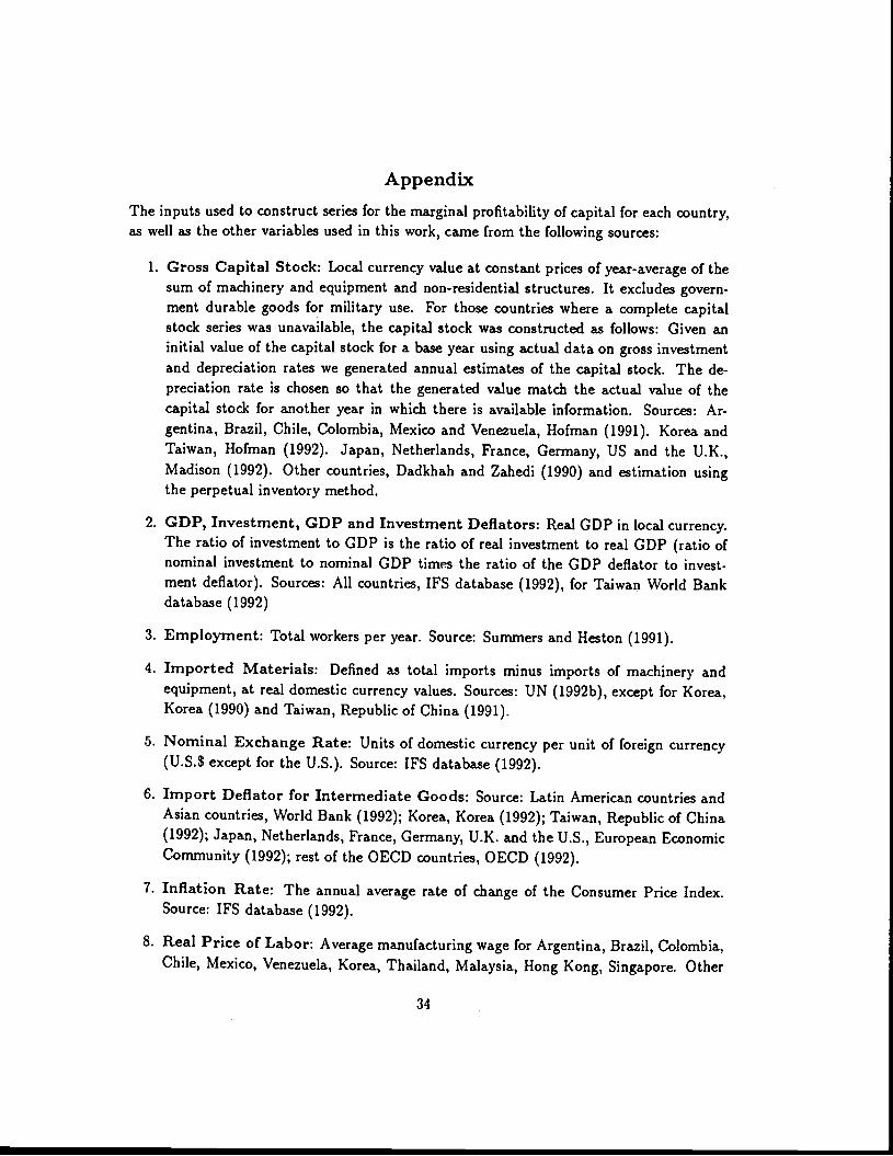
AppendixThe inputs used to construct series for the marginal profitability of capital for each country,as well as the other variables used in this work, came from the following sources:

1. Gross Capital Stock: Local currency value at constant prices of year-average of thesum of machinery and equipment and non-residential structures. It excludes govern-ment durable goods for military use. For those countries where a complete capitalstock series was unavailable, the capital stock was constructed as follows: Given aninitial value of the capital stock for a base year using actual data on gross investmentand depreciation rates we generated annual estimates of the capital stock. The de-preciation rate is chosen so that the generated value match the actual value of thecapital stock for another year in which there is available information. Sources: Ar-gentina, Brazil, Chile, Colombia, Mexico and Venezuela, Hofman (1991). Korea andTaiwan, Hofman (1992). Japan, Netherlands, France, Germany, US and the U.K.,Madison (1992). Other countries, Dadkhah and Zahedi (1990) and estimation usingthe perpetual inventory method.

2. GDP, Investment, GDP and Investment Deflators: Real GDP in local currency.The ratio of investment to GDP is the ratio of real investment to real GDP (ratio ofnominal investment to nominal GDP times the ratio of the GDP deflator to invest-ment deflator). Sources: All countries, IFS database (1992), for Taiwan World Bankdatabase (1992)

3. Employment: Total workers per year. Source: Summers and Heston (1991).

4. Imported Materials: Defined as total imports minus imports of machinery andequipment, at real domestic currency values. Sources: UN (1992b), except for Korea,Korea (1990) and Taiwan, Republic of China (1991).

5. Nominal Exchange Rate: Units of domestic currency per unit of foreign currency(U.S.$ except for the U.S.). Source: IFS database (1992).

6. Import Deflator for Intermediate Goods: Source: Latin American countries andAsian countries, World Bank (1992); Korea, Korea (1992); Taiwan, Republic of China(1992); Japan, Netherlands, France, Germany, U.K. and the U.S., European EconomicCommunity (1992); rest of the OECD countries, OECD (1992).

7. Inflation Rate: The annual average rate of change of the Consumer Price Index.Source: IFS database (1992).

8. Real Price of Labor: Average manufacturing wage for Argentina, Brazil, Colombia,Chile, Mexico, Venezuela, Korea, Thailand, Malaysia, Hong Kong, Singapore. Other

34

developing countries, average non-agriculture wage. For OECD countries, the realcompensation per employee. Deflated by the GDP deflator. Sources: ECLAC (1992),EEC (1992), UN (1992a).

9. Real Price of Imported Materials: For Latin American and Asian countries, nom-inal exchange rate times dollar price of imported goods divided by GDP deflator. ForOECD, implicit deflator for imported intermediate goods deflated by the GDP deflator.Sources: IFS data base, EEC (1992).

10. Real Exchange Rate: Nominal exchange rate times a trade weighted price index ofexported and imported goods divided by the GDP deflator. Source: IFS database.

11. Labor and Capital Shares: Factor shares in GDP are at factor cost net of capitalconsumption and indirect taxes. Sources: Argentina, Brazil, Chile, Colombia, Mexicoand Venezuela, ECLAC (1991). Korea and Taiwan, Korea (1992) and Republic ofChina (1989), respectively. France, Germany, Japan, Netherlands, UK, U.S., EuropeanEconomic Community (1992a). Other countries, United Nations, (1992).

12. Public and Private Investment: Public investment is investment of general govern.ment. Private investment is calculated as the difference between total fixed investmentfrom national accounts and public investment. Sources: OECD (1992) for OECDcountries, World Bank (1992) and Pfeffermandn and Madarassy (1993) for developingcountries.

13. Political Variables: PROB is the annual probability of a change in government, es-timated by a probit model on time series-data for the period 1948-1982, from Cukier-man, Edwards, and Tabellini (1992). ASSASS, CONCHG, CRISIS, REVOL, RIOT,and STRIKE are defined in Tables 5 and 6, and are from Barro and Wolf (1991).

35

References

Abel, Andrew B., "Optimal Investment Under Uncertainty," American Economic Review,March 1983, 73, 228—33.

Abel, Andrew B., and Olivier J. Blanchard, "The Present Value of Profits and Cyclical

Movements in Investment," Econometrica, March 1986, 54, 249—273.

Aizenman, Joshua, and Nancy Marion, "Policy Uncertainty, Persistence and Growth," NBER

Working Paper No. 3848, Sept. 1991.

Barro, Robert, and Holger Wolf, Data Appedix for "Economic Growth in a Cross Section of

Countries," Mimeo, 1991.

Bernanke, Ben S., "Irreversibility, Uncertainty, and Cyclical Investment," Quarterly Journalof Economics, Feb. 1983, 98, 85—106.

Bertola, Giuseppe, "Irreversible Investment," unpublished working paper, Princeton Univ.,1989.

Bertola, Giuseppe, and Ricardo Caballero "Irreversibility and Aggregate Investment," un-

published, Princeton University, 1990.

Bruno, Michael, Stanley Fischer, Elhanan Helpman, Nissan Liviatan, and Liora Meridor(eds.), Lessons of Economic Stabilization and its Aftermath, The MIT Press, 1991.

Bruno, Michael, and Liora Meridor, "The Costly Transition from Stabilization to Sustainable

Growth: Israel's Case," in M. Bruno et. al. (eds.), Lessons of Economic Stabilizationand its Aftermath, The MIT Press, 1991.

Caballero, Ricardo J., "On the Dynamics of Aggregate Investment," Columbia University,

Discussion Paper No. 541, May 1991.

Caballero, Ricardo J., "A Fallacy of Composition," American Economic Review, 1992.

Caballero, Ricardo J., and Robert S. Pindyck, "Uncertainty, Investment, and Industry Evo-

lution," NBER Working Paper No. 4160, September 1992.

Collins, Susan, and W. Park, "External Debt and Macroeconomic Performance in Korea,"

in J. Sachs (ed.) Developing Count nj Debt and The World Economy, TheUniversity ofChicago Press, 1989.

Corbo, Vit.torio, and Andrés Solimano, "Chile's Experience with Stabilization Revisited,"

Chapter 3 of M. Bruno, et. al. (eds.), Lessons of Economic Stabilization and its After-math, The MIT Press, 1991.

36

Corden, M., "Macroeconomic Policy and Growth: Some Lessons From The Experience,"

Annual Conference on Development Economics, The World Bank, 1990, 59-84.

Cukierman, Alex, "The Effects of Uncertainty on Investment under Risk Neutrality with

Endogenous Information," Journal of Political Economy, June 1980, 88, 462—475.

Cukierman, Alex, Sebastian Edwards, and Guido Tabellini, "Seigniorage and Political In-

stability," American Economic Review, June 1992, 82, 537—555.

Dixit, Avinash, "Entry and Exit Decisions under Uncertainty," Journal of Political Economy,

June 1989, 97, 620—638.

Dixit, Avinash, "Irreversible Investment with Price Ceilings," Journal of Political Economy,

June 1991b, 99, 541—557.

Dixit, Avinash, "Investment and Hysteresis," Journal of Economic Perspectives, Winter1992, 6, 107—132.

Dixit, Avinash, and Robert S. Pindyck, Investment under Uncertainty, forthcoming, Prince-

ton University Press, 1993.

Dornbusch, Rudiger, "Policies to Move From Stabilization to Growth," Annual Conference

on Development Economics, The World Bank, 1990, 19—48.

Dornbusch, Rudiger, and Stanley Fischer, "Stopping Hyperinflation: Past and Present,"NBER Working Paper No. 1810, 1986.

Dornbusch, Rudiger, and Stanley Fischer, "Moderate Inflation," The World Bank EconomicReview, Jan. 1993, 7, 1—44.

ECLAC, Statistical Yearbook for Latin America and the Caribbean, United Nations, various

issues, 1992.

EEC, The European Economy, Commission of the European Communities, Directorate Gen-

eral for Economic and Financial Affairs, various issues, 1992.

Edwards, Sebastian, and Felipe Larrain, Debt, Adjustment, and Recovery: Latin America 's

Prospects for Growth and Development, Cambridge: Basil Blackwell, 1989.

Fischer, Stanley, Indexing, Inflation and Economic Policy, MIT Press, 1986.

Fischer, Stanley, "Macroeconomics, Development and Growth" NBER Macroeconomics An-

nual, 1991.

Fischer, Stanley, "Macroeconomic Factors in Growth," paper presented at World Bank Con-

ference on How National Policies Affect Growth, Feb., 1993.

37

Hartman, Richard, "The Effects of Price and Cost Uncertainty on Investment," Journal of

Economic Theory, Oct. 1972, 5, 258-266.

Giovannini, Alberto, "The Interest Elasticity of Savings in Developing Countries: The Ex-

isting Evidence," World Development, 1983, 11, 601—607.

Hofman, Andre, "The Role of Capital in Latin America: A Comparative Perspective of Six

Countries for 1950-1989," ECLAC, Economic Development Division Working Paper No.

4, 1991.

Hofman, Andre, "Preliminary Estimates of Capital Stock for Korea and Taiwan," ECLAC,Economic Development Division mimeo, 1992.

Hull, John, and Alan White, "The Pricing of Options on Assets with Stochastic Volatilities,"

Journal of Finance, June 1987, 42, 281—300.

IMF, International Financial Statistics, Database, 1992.

Ingersoll, Jonathan E., Jr., and Stephen A. Ross. "Waiting to Invest: Investment andUncertainty," Journal of Business, Jan. 1992.

Kiguel, Miguel, and Nissan Liviatan, "When Do Heterodox Programs Work? Lessons From

Experience," The World Bank Research Observer, January 1992, 7, 35—57.

Korean Ministry of Planning, Statistical Yearbook, 1990.

Korea, Bank of Korea, Statistical Yearbook, 1992.

Kormendi, Roger, and Philip Meguire, "Macroeconomic Determinants of Growth: Cross

Country Evidence," Journal of Monetarj Economics, Sept., 1985, 16, 141—163.

Lach, Saul, and Rafael Rob, "R&D, Investment, and Industry Dynamics," NBER Working

Paper No. 4060, April 1992.

Lach, Saul, and Mark Schankerman, "Dynamics of R&D and Investment in the Scientific

Sector," Journal of Political Economy, August 1989, 97, 880—904.

Leahy, John, "The Optimality of Myopic Behavior in a Competitive Model of Entry and

Exit," Discussion Paper No. 1566, Harvard University, August 1991.

Levine, Ross, and David Renelt, "A Sensitivity Analysis of Cross-Country Growth Regres-

sions," American Economic Review, Sept. 1992, 82, 942—963.

Lippman, Steven A., and R. P. Rumelt, "Demand Uncertainty and Investment in Industry-

Specific Capital," unpublished, UCLA, Sept. 1985.

Lustig, N. Mexico: The Remaking of an Economy, Brookings Institution, 1992.

38

Madison, Angus, "Standardized Estimates of Fixed Investment and Capital Stock at Con-

stant Prices: A Long-Run survey of six countries," University of Gronigen, mimeo,1992.

Majd, Saman, and Robert S. Pindyck, "Time to Build, Option Value, and Investment Dcci-

sions," Journal of Financial Economics, Mar. 1987, 18, 7—27.

McDonald, Robert, and Daniel R. Siegel, "The Value of Waiting to Invest," Quarterly Jour-

nal of Economics, Nov. 1986, 101, 707—728.

Morales, J.A., "The Transition Fom Stabilization to Sustained Growth in Bolivia," in M.

Bruno et al. (eds.), Lessons of Economic Stabilization and its Aftermath, The MITPress, 1991.

OECD, National Accounts, Paris, France: OECD Department of Economics and Statistics,1992.

Ortiz, G., "Mexico Beyond the Debt Crisis: Towards Sustainable Growth with Price Stabil-

ity," in M. Bruno et. al. (eds.), Lessons of Economic Stabilization and its Aftermath,The MIT Press, 1991.

Pfefferman, C., and A. Madarassy, "Trends in Private Investment in Developing Countries."

Discussion Paper No. 14, IFC, The World Bank, 1992.

Pindyck, Robert S., "Irreversible Investment, Capacity Choice, and the Value of the Firm,"

American Economic Review, Dec. 1988, 79, 969—985.

Pindyck, Robert S., "Irreversibility, Uncertainty, and Investment," Journal of EconomicLiterature, September 1991, 29, 1110—1152.

Pindyck, Robert S., "A Note on Competitive Investment under Uncertainty," AmericanEconomic Review, March 1993, 83, 273—77.

Republic of China, National Income in Taiwan, Directorate General of Budget, Accounting,

and Statistics, DGBAS, 1989.

Republic of China, Statistical Yearbook, Directorate General of Budget, Accounting, and

Statistics, DOBAS, 1991.

Rodrik, Dani, "Policy Uncertainty and Private Investment in Developing Countries," NBER

Working Paper No. 2999, June 1989.

Sachs, Jeffrey E. (ed.), Developing Country Debt and the World Economy, The University

of Chicago Press, 1989.

39

Schmidt-Hebbel, Klaus, Steven B. Webb, and Giancarlo Corsetti, "Household Savings in De-

veloping Countries: First Cross-Country Evidence," The World Bank Economic Review,

September 1992, 6, 529—547.

Scott, Louis 0., "Option Pricing When the Variance Changes Randomly: Theory, Estima-tion, and an Application," Journal of Financial and Quantitative Analysis, Dec. 1987,22, 419—438.

Serven, Luis, and Andrés Solimano, "Private Investment and Macroeconomic Adjustment:

A Survey," The World Bank Research Observer, January 1992, 7, 95—114.

Serven, Luis, and Andrés Solimano, "Debt Crisis, Adjustment Policies, and Capital For-mation in Developing Countries: Where Do We Stand?" World Development, January

1993, 21, 127—140.

Solimano, Andrés, "Inflation and the Costs of Stabilization: Historical and Recent Experi-

ences and Policy Lessons," The World Bank Research Observer, July 1990, 5, 167—185.

Solimano, Andrés, "Understanding the Investment Cycle in Adjustment Programs: Evidence

From Reforming Economies," PRE Working Paper No. 912, June 1992, The WorldBank.

Solimano, Andrés, "How Private Investment Reacts to Changing Macroeconomics Condi-

tions: The Case of Chile in the 1980s," in A. Chhibber, M. Dailami and N. ShaIIk

(eds.), Reviving Private Investment in Developing Countries: Empirical Studies and

Policy Lessons, North-Holland, 1992.

Summers, Robert, and Alan Heston, "The Penn World Table (Mark 5): An Expanded Set

of International Comparisons, 1950-1988," Quarterly Journal of Economics, 1991, 327-367.

United Nations, Statistical Yearbook, 1992.

United Nations, Commission of Trade Database, Statistics Office, 1992.

Wiggins, James B., "Option Values Under Stochastic Volatility," Journal of Financial Eco-

nomics, 1987, 19, 351—372.

World Bank, BESD Database, 1992.

40

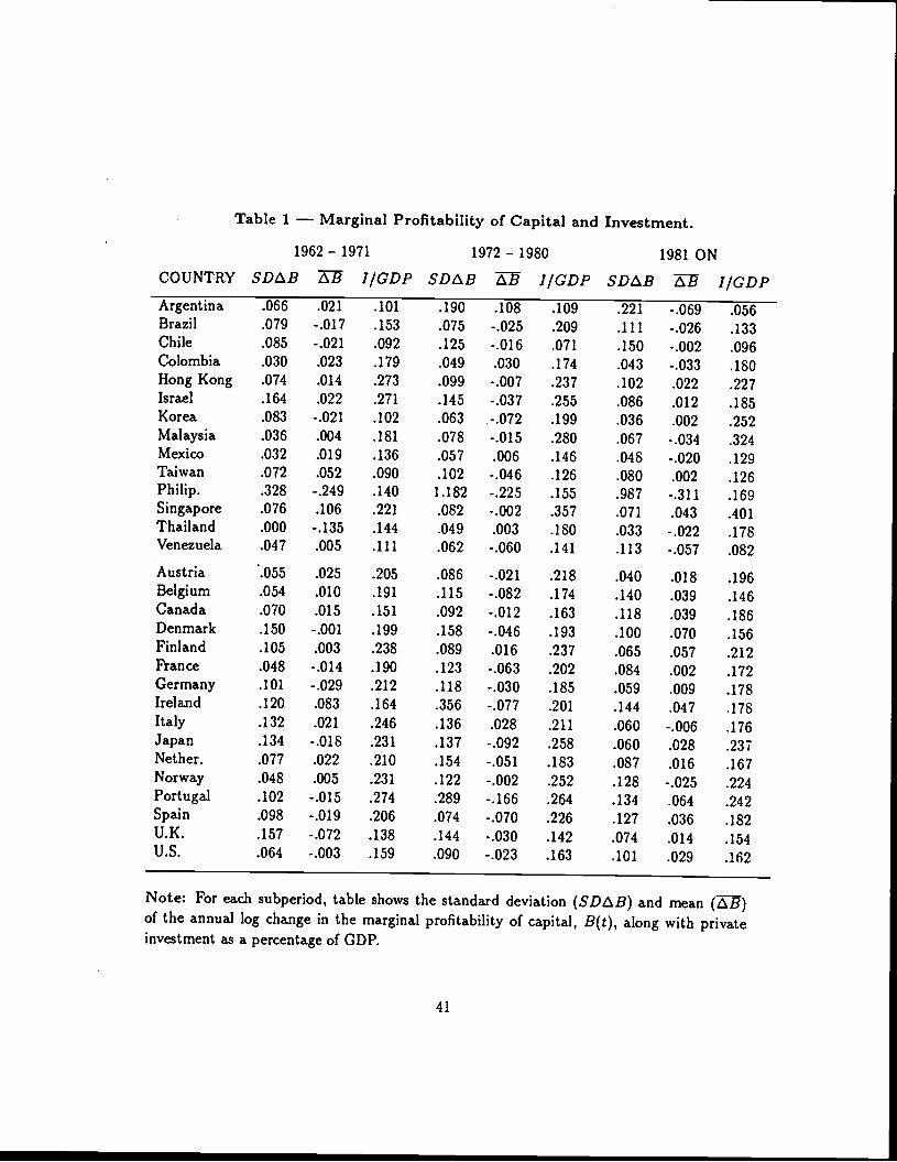
AustriaBelgiumCanadaDenmarkFinlandFranceGermanyIrelandItalyJapanNether.NorwayPortugalSpainU.K.U.S.

Note: For each subperiod, table shows the standard deviation (SDiB) and mean ()of the annual log change in the marginal profitability of capital, B(t), along with privateinvestment as a percentage of GDP.

41

Table 1 — Marginal Profitability of Capital and Investment.1962 — 1971 1972 — 1980 1981 ON

COUNTRY SDE,B H I/GDP SDiB 3 I/GDP SDEB I/GDPArgentinaBrazilChileColombiaHong KongIsraelKoreaMalaysiaMexicoTaiwanPhilip.SingaporeThailandVenezuela

.066 .021 .101

.079 -.017 .153

.085 -.021 .092

.030 .023 .179.074 .014 .273.164 .022 .271.083 -.021 .102.036 .004 .181.032 .019 .136.072 .052 .090.328 -.249 .140.076 .106 .221.000 -.135 .144.047 .005 .111

.055 .025 .205

.054 .010 .191

.070 .015 .151

.150 -.001 .199

.105 .003 .238

.048 -.014 .190

.101 -.029 .212.120 .083 .164.132 .021 .246.134 -.018 .231.077 .022 .210.048 .005 .231.102 -.015 .274.098 -.019 .206.157 -.072 .138.064 -.003 .159

.190 .108 .109.075 -.025 .209.125 -.016 .071.049 .030 .174.099 -.007 .237.145 -.037 .255.063 -.072 .199.078 -.015 .280.057 .006 .146.102 -.046 .126

1.182 -.225 .155.082 -.002 .357.049 .003 .180.062 -.060 .141

.086 -.021 .218

.115 -.082 .174

.092 -.012 .163

.158 -.046 .193

.089 .016 .237.123 -.063 .202.118 -.030 .185.356 -.077 .201.136 .028 .211.137 -.092 .258.154 -.051 .183.122 -.002 .252.289 -.166 .264.074 -.070 .226.144 -.030 .142.090 -.023 .163

.221 -.069

.111 -.026.150 -.002.043 -.033.102 .022.086 .012.036 .002.067 -.034.048 -.020.080 .002.987 -.311.071 .043.033 -.022.113 -.057

.040 .018

.140 .039

.118 .039

.100 .070.065 .057.084 .002.059 .009.144 .047.060 -.006.060 .028.087 .016.128 -.025.134 .064.127 .036.074 .014.101 .029

.056

.133

.096.180.227.185.252.324.129.126.169.401.178.082

.196

.146

.186

.156

.212.172.178.178.176.237.167.224.242.182.154.162

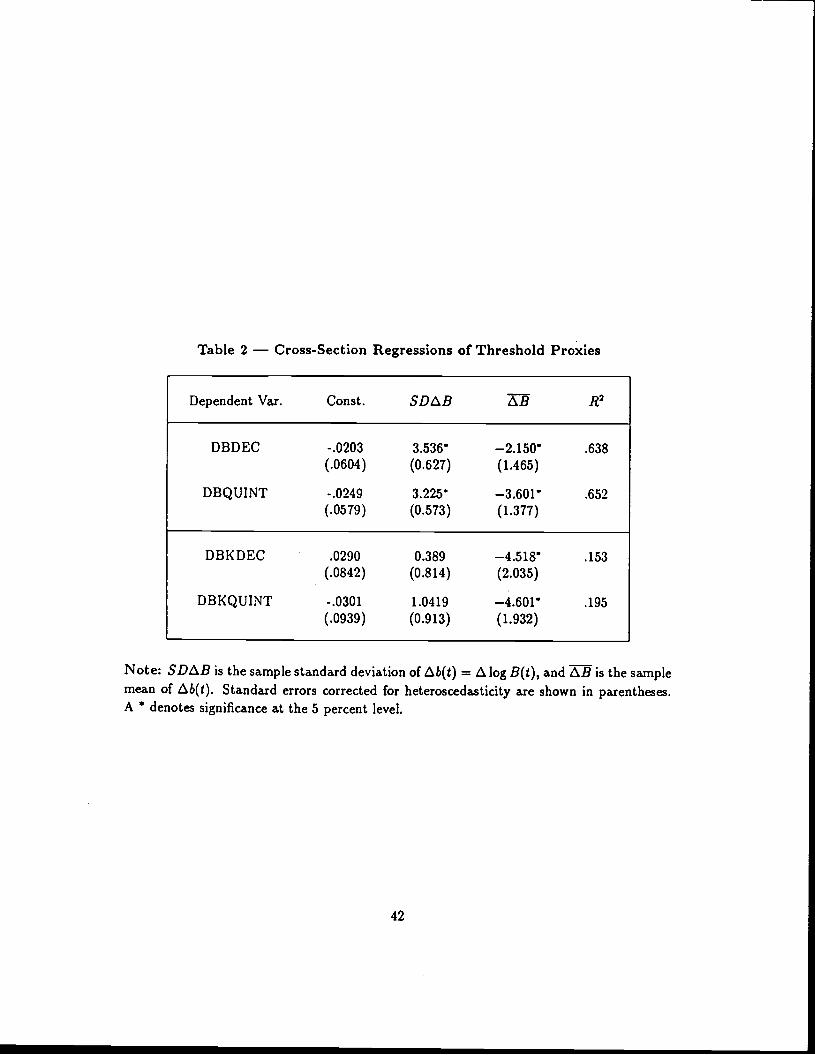
Table 2 — Cross-Section Regressions of Threshold Proxies

Dependent Var. Const. SDB ft2

DBDEC -.0203 3.536 —2.150 .638(.0604) (0.627) (1.465)

DBQUINT -.0249 3.225 —3.601 .652(.0579) (0.573) (1.377)

DBKDEC .0290 0.389 —4.518 .153(.0842) (0.814) (2.035)

DBKQUINT -.0301 1.0419 —4.601 .195(.0939) (0.913) (1.932)

Note: SDiB is the sample standard deviation of ib(t) = i log B(i), and is the samplemean of b(t). Standard errors corrected for heterosceda.sticity are shown in parentheses.A * denotes significance at the 5 percent level.

42

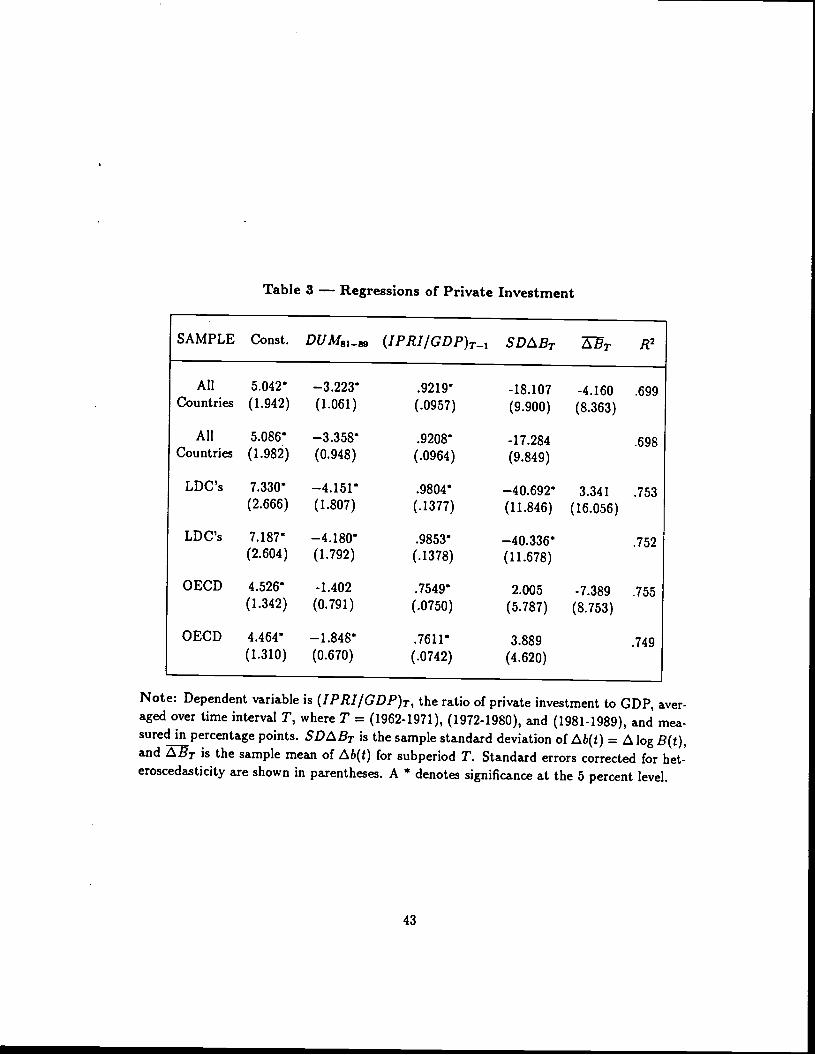
Table 3 — Regressions of Private Investment

SAMPLE Const. DUM81 (IPRI/GDP)T..1 SDtBT R2

All 5.042 —3.223 .9219 -18.107 -4.160 .699Countries (1.942) (1.061) (.0957) (9.900) (8.363)

All 5.086 —3.358 .9208 -17.284 .698Countries (1.982) (0.948) (.0964) (9.849)

LDC's 7.330 —4.151 .9804 —40.692 3.341 .753(2.666) (1.807) (.1377) (11.846) (16.056)

LDC's 7.187 —4.180 .9853 —40.336 .752(2.604) (1.792) (.1378) (11.678)

OECD 4.52& -1.402 .7549 2.005 -7.389 .755(1.342) (0.791) (.0750) (5.787) (8.753)

OECD 4.464 —1.848 .7611 3.889 .749(1.310) (0.670) (.0742) (4.620)

Note: Dependent variable is (IPRI/GDP)T, the ratio of private investment to GDP, aver-aged over time interval T, where T = (1962-1971), (1972-1980), and (1981-1989), and mea-sured in percentage points. SDB is the sample standard deviation ofzb(t) = i logB(t),and L.BT is the sample mean of b(i) for subperiod T. Standard errors corrected for het-eroscedasticity are shown in parentheses. A * denotes significance at the 5 percent level.

43

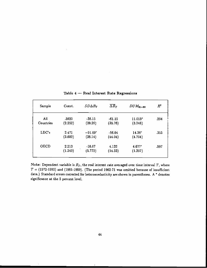
Table 4 — Real Interest Rate Regressions

Sample Const. SD.BT LBT DUM81.89 R2

All .5930 .38.15 -61.15 11.015 .294Countries (2.252) (20.26) (35.76) (3.248)

LDC's 2.471 —91.69 -56.04 14.38 .353

(3.602) (38.14) (44.04) (4.704)

OECD 2.213 -10.67 4.132 4.677 .597

(1.249) (5.772) (14.33) (1.397)

Note: Dependent variable is RT, the real interest rate averaged over time interval T, whereT = (1972-1980) and (1981-1989). (The period 1962-71 was omitted because of insufficientdata.) Standard errors corrected for heteroscedasticity are shown in parentheses. A *denotessignificance at the 5 percent level.

44

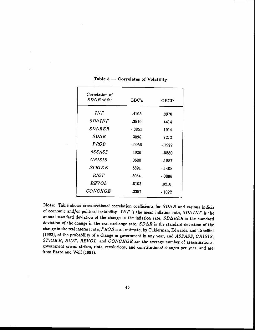
Table 5 — Correlates of Volatility

Correlation ofSDEB with: LDC's OECD

INF .4105 .3970

SDEilNF .3816 .4414

SDSRER -.0851 .1014

SDIR .3096 .7213

PROB -.0056 -.1922

ASSASS .4026 -.0580

CRISIS .0680 -.1887

STRIKE .5891 -.1408

RIOT .5054 - .0806

RE VOL -.0103 .0210

CONCHGE -.2357 -.1022

Note: Table shows cross-sectional correlation coefficients for SDB and various indiciaof economic and/or political instability. INF is the mean inflation rate, SDLilNF is theannual standard deviation of the change in the inflation rate, SDIRER is the standarddeviation of the change in the real exchange rate, SDR is the standard deviation of thechange in the real interest rate, PROB is an estimate, by Cukierman, Edwards, and Tabellini(1992), of the probability of a change in government in any year, and ASSASS, CRISIS,STRIKE, RIOT, REVOL, and CONCHGE are the average number of assassinations,government crises, strikes, riots, revolutions, and constitutional changes per year, and arefrom Barro and Wolf (1991).

45

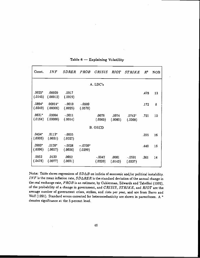
Table 6 — Explaining Volatility

Const. INF SDRER PROB CRISIS RIOT STRIKE R2 NOB

A. LDC's

.0625 .00020 .0017 .478 13(.0145) (.00012) (.0019)

.0894 .00014 -.0010 -.0509 .172 8(.0349) (.00006) (.0025) (.0578)

.0631 .00004 -.0011 .0076 .0074 .0743 .721 10(.0164) (.00008) (.0014) (.0565) (.0085) (.0268)

B. OECD

.0454 .0113 -.0005 .395 16(.0303) (.0031) (.0027)

.0903 .0120 -.0028 —.0700 .440 16(.0396) (.0027) (.0036) (.0299)

.0052 .0 139 .0052 -.0042 .000 1 -.0591 .361 14(.0478) (.0077) (.0031) (.0220) (.0143) (.0337)

Note: Table shows regressions of SDLB on indicia of economic and/or political instability.INF is the mean inflation rate, SDtRER is the standard deviation of the annual change inthe real exchange rate, PROB is an estimate, by Cukierman, Edwards and Tabellini (1992),of the probability of a change in government, and CRISIS, STRIKE, and RIOT are theaverage number of government crises, strikes, and riots per year, and are from Barro andWolf (1991). Standard errors corrected for heteroscedasticity are shown in parentheses. A *denotes significance at the 5 percent level.

46

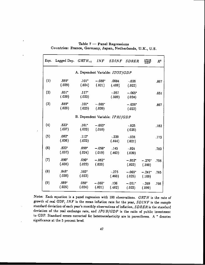
Table 7 — Panel RegressionsCountries: France, Germany, Japan, Netherlands, U.K., U.S.

Eqn. Lagged Dep. GRTJL1 INF SDINF SDRER R2

A. Dependent Variable: ITOT/GDP

(1) .889 .101 —.088 .0004 -.038 .867(.029) (.024) (.021) (.489) (.022)

(2) .851 .117 -.057 —.065 .851(.030) (.023) (.509) (.024)

(3) .889 .101 —.088 —.038 .867(.029) (.023) (.020) (.022)

B. Dependent Variable: IPRI/GDP

(4) .833 .101 —.053 -.025 .782(.037) (.023) (.018) (.020)

(5) .082 .112 -.220 .038 .773(.036) (.023) (.444) (.021)

(6) .833* .099 —.056 .145 .024 .783(.037) (.024) (.019) (.463) (.020)

(7) .890 .090 —.062 —.052 —.270 .798(.038) (.022) (.020) (.023) (.100)

(8) .848 .103 -.275 —.065 —.241 .785(.038) (.023) (.460) (.025) (.100)

(9) .889 .088 —.065 .136 —.051 -.269 .798(.029) (.024) (.021) (.482) (.023) (.099)

Note: Each equation is a panel regression with 180 observations. GRTH is the rate ofgrowth of real GDP, INF is the mean inflation rate for the year, SDINF is the samplestandard deviation of each year's monthly observations of inflation, SDRER is the standarddeviation of the real exchange rate, and JPUB/GDP is the ratio of public investmentto GDP. Standard errors corrected for heteroscedasticity are in parentheses. A * denotessignificance at the 5 percent level.

47

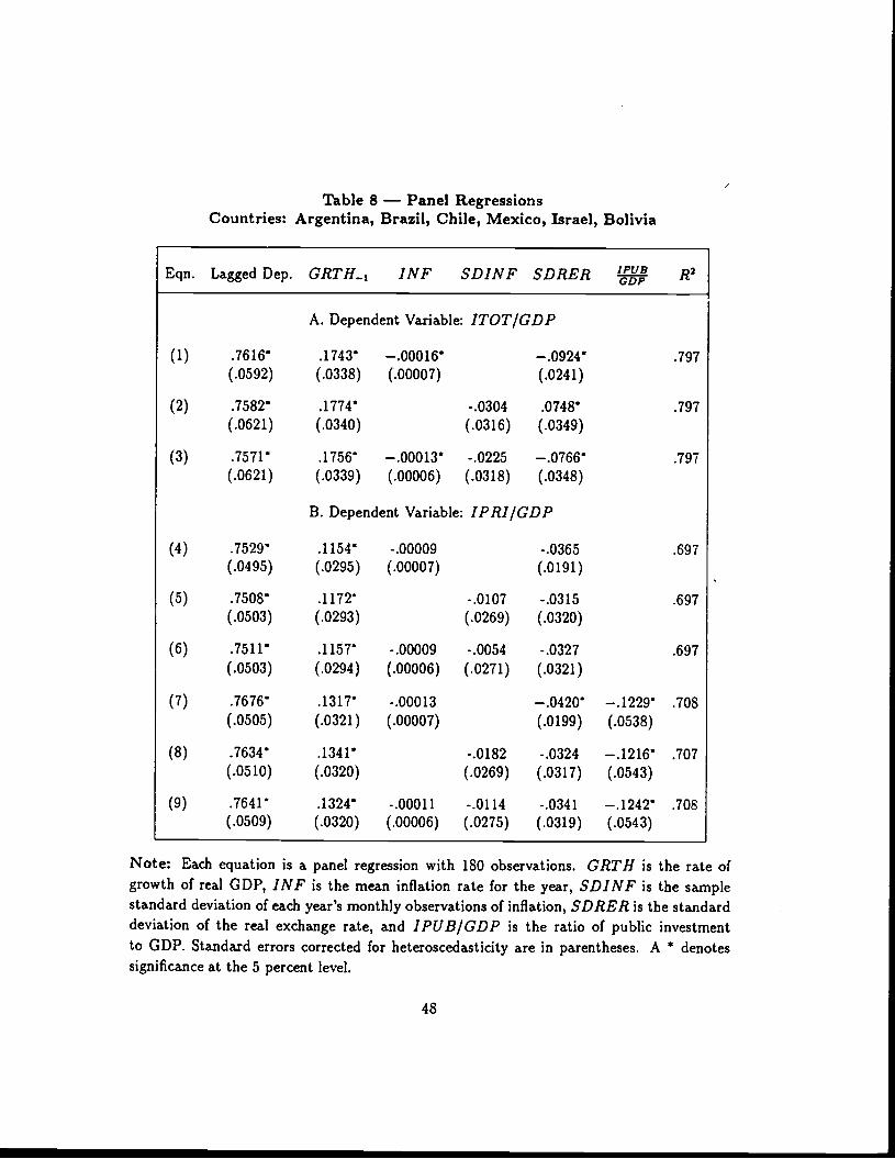
Table 8 — Panel RegressionsCountries: Argentina, Brazil, Chile, Mexico, Israel, Bolivia

Eqn. Lagged Dep. GRTH.1 INF SDINF SDRER

A. Dependent Variable: ITOT/GDP

(1) .7616' .1743' —.00016' —.0924' .797(.0592) (.0338) (.00007) (.0241)

(2) .7582' .1774' -.0304 .0748' .797(.0621) (.0340) (.0316) (.0349)

(3) .7571' .1756' —.00013' -.0225 —.0766' .797(.0621) (.0339) (.00006) (.0318) (.0348)

B. Dependent Variable: IPRI/GDP

(4) .7529' .1154' -.00009 -.0365 .697(.0495) (.0295) (.00007) (.0191)

(5) .7508' .1172' -.0107 -.0315 .697

(.0503) (.0293) (.0269) (.0320)

(6) .7511' .1157' -.00009 -.0054 -.0327 .697(.0503) (.0294) (.00006) (.0271) (.0321)

(7) .7676 .1317' -.00013 —.0420' —.1229' .708(.0505) (.0321) (.00007) (.0199) (.0538)

(8) .7634' .1341' -.0182 -.0324 —.1216' .707(.0510) (.0320) (.0269) (.0317) (.0543)

(9) .7641' .1324' -.00011 -.0114 -.0341 —.1242' .708(.0509) (.0320) (.00006) (.0275) (.0319) (.0543)

Note: Each equation is a panel regression with 180 observations. GRTH is the rate ofgrowth of real GDP, INF is the mean inflation rate for the year, SDINF is the samplestandard deviation of each year's monthly observations of inflation, SDRER is the standarddeviation of the real exchange rate, and IPUB/GDP is the ratio of public investmentto GD?. Standard errors corrected for heteroscedasticity are in parentheses. A * denotessignificance at the 5 percent level.

48

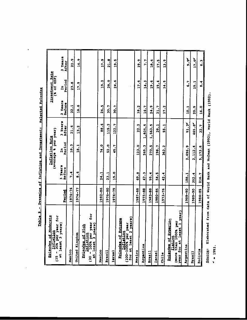
Table 9 — D

ynam

ics of Inf1atjo and Investment:

Selected Episodes

EPisode. of Moderate

Period

Inflation Rate

(average % per ye

ar)

3 Years

In

3 Years

Before

Period

Investment Rate

(% of GDP)

3 Years

In

3 Years

Inflation

(15 — 30% per ye

ar f

or

at least 3 years)

Mexico

1974—76

7.4

18.3

21.6

Before

Period

After

United Kingdom

1974—77

8.6

18.1

23.8

22.9

Eieodes of High

Inflation

(30 — 100% per y

ear for

at least 3 years)

13.2

18.8

17.9

16.9

Mexico

1982—86

24.1

Brazil

1976—80

74.0

88.6

23.1

52.0

26.5

19.2

17.9

Israel

1974—79

115.2

15.0

45.7

30.7

28.0

21.8

Episodes of

30.7

24.6

19.5

:

Extreme

Inflation

(100—1000% per ye

ar

for at least 2 years)

Mexico

1987—88

69.8

123.0

Argentina

1975—88

22.2

47.3

18.2

17.6

19.9

Brazil

1983—88

1,835.5

95.4

270.5

16.7

14.3

7.7

Israel

1980—85

1,563.5

54.5

24.9

19.6

18.6

Chile

1973—76

28.1

42.4

363.2

21.7

19.4

17.5

EDisodes of Hv'perjn—

55.1

17.2

14.5

13.9

flation

(more than 1000% per

year

for at least 1 year)

Argentina

1989—90

188.1

2,696.9

9l.3

Brazil

1989—90

352.4

2,112.4

465•8W

10.1

6.7

9.9'

Bolivia

1984—85

216.7

5,173.8

32.7

20.9

19.1

Source:

Elaborated from data of World Bank and Hofman (1992), World Bank (1992).

—

1991

.

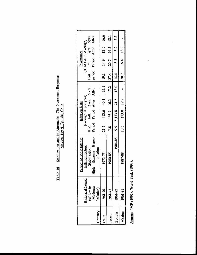
Tab

le 1

0 -

Sta

biliz

atio

n an

d its

Afte

rmat

h: T

he I

nves

tmen

t R

espo

nse.

M

exic

o. I

srae

l. B

oliv

ia.

Chi

le

Cou

ntry

His

tori

cal

Peri

od

Peri

od o

f M

ost

Inte

nse

Infl

atio

n R

ate

(ave

rage

% p

er y

ear)

H

ist.

InfI

. 3y

rs.

5 yr

s.

Peri

od

Peri

od

Aft

er

Aft

er

Inve

stm

ent

(% o

f GD

P, A

vera

ge)

His

t. In

fi.

3yrs

. 5y

rs.

peri

od

Peri

od

Aft

er

Aft

er

Infl

atio

n be

fore

St

abili

zatio

n H

igh

Ext

rem

e H

yper

- in

flat

ion

(of

low

to

Mod

erat

e In

flat

ion)

Chi

le

1961

-70

1973

-75

27.2

41

3.6

40.1

35

.1

19.1

14

.9

13.6

16

.6

Isra

el

1961

-73

1980

-85

7.8

198.

7 16

.3

17.2

27

.4

20.7

16

.5

18.1

Bol

ivia

19

61-7

2 19

84-8

5 5.

5 5,

173.

8 21

.5

18.0

14

.4

5.3

5.9

5.3

Mex

ico

1961

-81

1987

-88

10.6

12

3.0

19.9

-

20.7

16

.4

18.9

-

Sour

ce:

IMF

(199

2),

Wor

ld B

ank

(199

2).

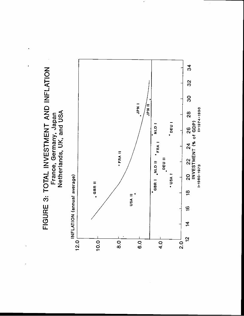
12.0

10.0

8.0-

FIG

UR

E 3

: T

OT

AL

IN V

ES

TM

EN

T A

ND

IN

FLA

TIO

N

Fra

nce,

Ger

man

y, J

apan

N

ethe

rland

s, U

K,

and

US

A

INF

LAT

ION

(an

nual

ave

rage

)

6.0-

4.0

2.0 12

14

16

18

20

22

24

IN

VE

ST

ME

NT

(%

1-

1960

-197

3

30

32

34

• G

BR

II

• F

AA

II

JPN

I

U

US

A

II

• U

GB

R I

•NLD

II

- N

LD I

F

RA

I

DE

U I

I U

U

US

AI

DE

UI

I I

I 26

28

of G

OP

) 11

-197

4-19

90

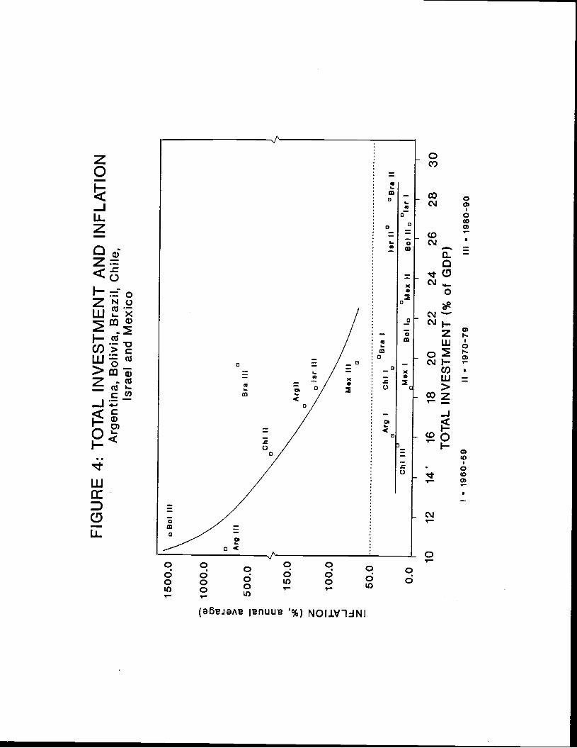
1500

.0

FIG

UR

E 4

: T

OT

AL

IN V

ES

TM

EN

T

Arg

entin

a, B

oliv

ia,

Bra

zil,

Isra

el a

nd M

exic

o

AN

D I

NF

LAT

ION

C

hile

,

a,

0)

I-

a, >

C z 0 -J

LL z

Chi

III

M

ex

I B

ol I,

M

ex I

I B

ol h

o Ii

I

I I

I I

I I

I I

o B

ol I

II

a Arg

III

0 B

ra I

II

Chi

II

C

1000

.0

500.

0

150.

0

100.

0

50.0

0.0

A rg

I I

0 0

Is,

III

Mex

III

C

0 Arg

I

ChI

°B

ra I

he

r 11

0 °B

ra I

I

10

12

14

16

18

20

22

24

26

28

30

TO

TA

L IN

VE

ST

ME

NT

(% o

f G

DP

) I

• 19

60-6

9 II

- 19

70-7

9 III

- 1

980-

90

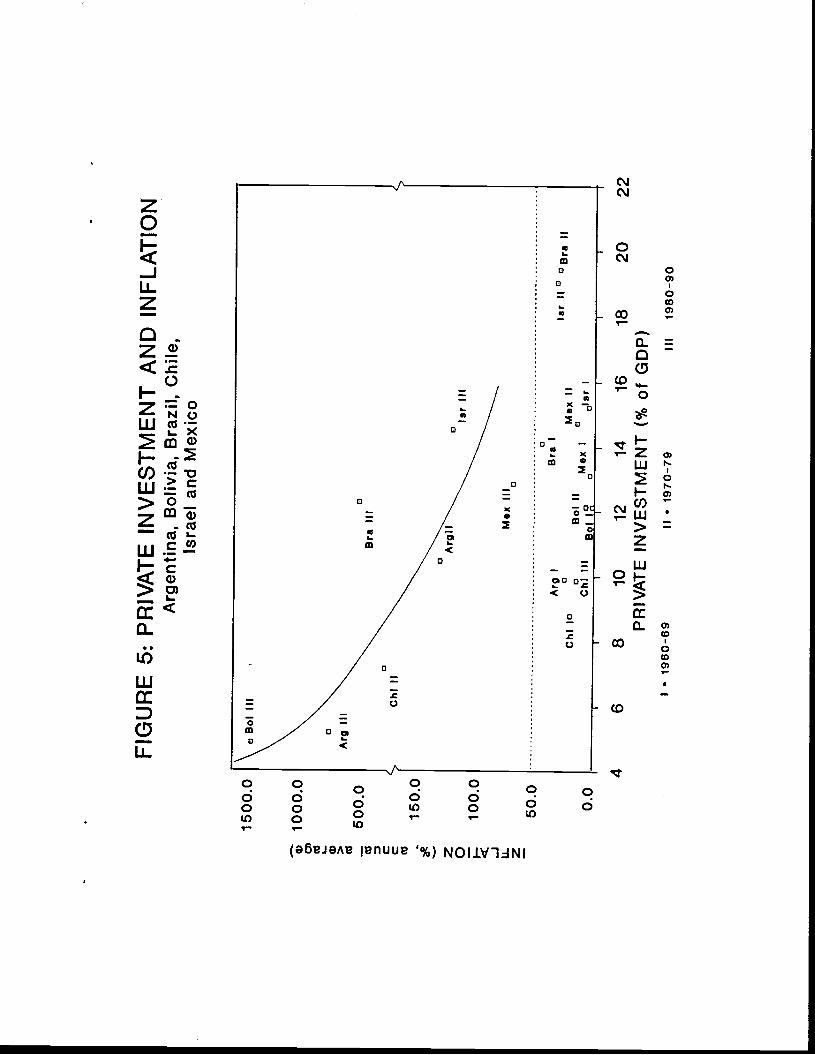
FIG

UR

E 5

: P

RIV

AT

E I

NV

ES

TM

EN

T A

ND

IN

FLA

TIO

N

Arg

entin

a, B

oliv

ia,

Bra

zil,

Chi

le,

Isra

el a

nd M

exic

o

a,

0)

a, I-

>

a,

a,

C

C

a, z 0 -J

Ii- z

1500

.0

1000

.0

500.

0

150.

0

100.

0

50.0

0.0

4 6

8 10

12

14

16

P

RIV

AT

E I

N V

ES

TM

EN

T (%

of

GD

P)

I •

1960

-69

II •

1970

-79

III

1980

-90

18

20

22