NBER WORKING PAPER SERIES ECONOMIC CONDITIONS, DETERRENCE AND JUVENILE … · · 1999-11-29NBER...

NBER WORKING PAPER SERIES

ECONOMIC CONDITIONS, DETERRENCE AND JUVENILECRIME: EVIDENCE FROM MICRO DATA

H. Naci MocanDaniel I. Rees

Working Paper 7405http://www.nber.org/papers/w7405

NATIONAL BUREAU OF ECONOMIC RESEARCH1050 Massachusetts Avenue

Cambridge, MA 02138October 1999

Paul Niemann provided excellent research assistance. Mocan gratefully acknowledges research support fromthe NBER. We thank Michael Grossman, Steve Levitt and the participants of the 1999 NBER SummerInstitute and CRESP Seminar on Labor and Human Resource Economics for helpful comments andsuggestions. The views expressed herein are those of the authors and not necessarily those of the NationalBureau of Economic Research.

© 1999 by H. Naci Mocan and Daniel I. Rees. All rights reserved. Short sections of text, not to exceed twoparagraphs, may be quoted without explicit permission provided that full credit, including © notice, is givento the source.

Economic Conditions, Deterrence and Juvenile Crime:Evidence from Micro DataH. Naci Mocan and Dainel I. ReesNBER Working Paper No. 7405October 1999JEL No. K42

ABSTRACT

This is the first paper to test the economic model of crime for juveniles using micro data.

It uses a nationally representative sample of 16,478 high school children surveyed in 1995. The

sample includes not only detailed information on offenses, but also data on personal, family and

neighborhood characteristics as well as deterrence measures. We analyze the determinants of selling

drugs, committing assault, robbery, burglary and theft, separately for males and females.

We find that an increase in violent crime arrests reduces the probability of selling drugs and

assaulting someone for males, and reduces the probability of selling drugs and stealing for females.

An increase in local unemployment increases the propensity to commit crimes, as does local poverty.

Similarly, family poverty increases the probability to commit robbery, burglary and theft for males,

and assault and burglary for females. Local characteristics are more important for females than males.

The results also indicate that family supervision has an impact on delinquent behavior.

These results show that juveniles do respond to incentives and sanctions as predicted by

economic theory. Employment opportunities, increased family income and more strict deterrence are

effective tools to reduce juvenile crime.

H. Naci Mocan Daniel I. ReesUniversity of Colorado at Denver University of Colorado at DenverDepartment of Economics Department of EconomicsCampus Box 181, PO Box 173364 Campus Box 181, PO Box 173364Denver, CO 80217-3364 Denver, CO 80217-3364and NBER [email protected]@carbon.cudenver.edu

1

Economic Conditions, Deterrence and Juvenile Crime:Evidence from Micro Data

I. Introduction

The American public ranked crime as the most important problem facing the

nation in 1999 (Gallup Organization, 1999). Juvenile crime, in particular, has

received a great deal of attention from the public, the media (Washington Post 1999,

Los Angeles Times 1999, Newsweek 1999), and social scientists. Some analysts

argue that very little, if anything, can be done to discourage young Americans from

participating in illegal activities. For example, DiIulio (1996) indicates that urban

ethnographers believe that today’s crime-prone youngsters are too present oriented for

any type of conventional criminal deterrence to work. Similarly, Bennett, DiIulio and

Walters (1996) state that “America is now home to thickening ranks of juvenile ‘super-

predators’—radically impulsive, brutally remorseless youngsters, including even more

preteenage boys, who murder, assault, rape, rob, burglarize, deal deadly drugs, join gun-

toting gangs, and create serious communal disorder. They do not fear the stigma of

arrest, the pains of imprisonment, or the pangs of conscience… To these mean-street

youngsters, the words ‘right’ and ‘wrong’ have no fixed moral meaning.”1

However, the notion of an irrational “new-breed” of juvenile criminal who does not

respond to incentives is based on anecdotal as opposed to strong empirical evidence.

Moreover, it contradicts the economic model of crime developed by Becker (1968) and

tested using aggregate data and micro data on the adult population (e.g., Witte 1980,

Cornwell and Trumbull 1994, Levitt 1997, Corman and Mocan, forthcoming). In recent

work, using state-level data, Levitt (1998) found that the juvenile crime rate is negatively

related to the severity of penalties, indicating that the economic model of crime applies to

juveniles as well as adults. Furthermore, the sharp increase in the juvenile crime in late-

1980s, and the drop in the mid-1990s implies that juvenile crime may be more malleable

than suggested.

1 Bennet, DiIulio and Walters (1996) as cited by Levitt (1998).

2

Investigation of the determinants of juvenile crime is important, not only

because of the nature of the problem, but also because of the implications of juvenile

crime for adolescents’ behavior in the future. For example, Mocan and Overland (1999)

show that current criminal activity makes future criminal activity more likely by

simultaneously increasing the criminal human capital of the participant and depreciating

his legal human capital, and Bound and Freeman (1992) document a negative

relationship between criminal participation and labor market attachment, stating that "…

the growth rate of the population with a criminal record accounts for one third of the

longer run erosion of employment [of black male high school dropouts].” In addition,

Freeman and Rodgers (1999) show that areas with the most rapidly rising rates of

incarceration are areas in which youths, particularly black youths, have had the worst

earning and employment experience between the mid 1980s and late 1990s, suggesting a

negative relationship between labor market outcomes and a criminal record.

There is no study in the economics literature that investigates the determinants of

juvenile crime using micro data, although three papers have analyzed the behavior of

young adults. Viscusi (1986) used data on 2,358 black men ages 16 to 24, living in

Boston, Chicago and Philadelphia in 1979. Tauchen, Witte and Griesinger (1994)

analyzed the criminal activity of 567 men ages 19-25 who were born in Philadelphia in

1945, and Grogger (1998) used the NLSY to investigate the determinants of criminal

behavior of 1,134 men ages 14-21 in 1980. Although these papers provide interesting

insights into the determinants of criminal activity for young adults, they all have

limitations. The Viscusi (1986) and Tauchen et al. (1994) samples are not nationally

representative, and all three papers lack good measures of criminal activity or legal

sanctions.2 Furthermore, none of these papers use data on recent cohorts, around whom

the current debate centers, and none specifically analyze juvenile delinquency.3

2 In Tauchen et al. (1994) criminal activity is measured by being arrested, or by a crime seriousnessindex. In Viscusi (1986) criminal activity is measured by committing any crime; and Grogger (1998)considers only property crimes. Viscusi (1986) and Grogger (1998) have no measures of deterrence.

3 Viscusi analyzes young adults who are born between 1955 and 1963; Grogger (1998)analyzes young adults whose birthdays are between 1959 and 1964, and Tauchen et al. (1994)sample uses young adults born in 1945.

3

The criminology literature on juvenile crime is more extensive, but it too has

limitations. Often the measure of criminal involvement is based on arrest records, or is

based on parent/teacher reports (Wright, Cullen and Williams, 1997). Most researchers

use either small samples (e.g. n=200 in Baron and Hartnagel 1997), or data from a

single city or region (e.g. data from Alberta, Canada in LaGrange and Silverman 1999;

Dunedin, New Zealand in Wright et al. 1999; Rochester, New York in Smith and

Thornberry 1995). No study simultaneously controls for the effects of economic and

deterrence variables as well as personal and family characteristics.

An ongoing debate in crime literature is the relative importance of labor market

opportunities and criminal sanctions on the level of criminal activity. Freeman (1983),

reviewed a number of studies employing measures of criminal sanctions and labor market

conditions. He concluded that sanctions have a greater impact on criminal behavior than

do labor market factors: that is, the “stick” seems to be more effective than the “carrot.”

The findings of Corman and Mocan’s recent time-series analysis (forthcoming) also

provide some support for this conclusion. They found that poverty is positively related to

homicides, but arrests and police force have a negative impact on a variety of criminal

activities. In contrast, researchers using data on prison releases have reported mixed

results with regard to the relative importance of deterrence versus labor market

opportunities (e.g. Witte 1980, Myers 1983). Information on the importance of

deterrence versus labor market conditions is absent for juvenile crime.

This paper presents the first economic analysis of juvenile crime using

individual-level data. The nationally representative sample includes not only detailed

information on offenses, but also data on personal, family and neighborhood

characteristics as well as deterrence measures. Because individual-level, as opposed to

aggregate data, are used, the estimated relationships between sanctions and criminal

activity represent the impact of deterrence. Put differently, they don’t suffer from

potential confounding of the incapacitation effect that necessarily emerges in aggregate

data (e.g., Corman and Mocan, forthcoming; Levitt, 1998). We analyze the

determinants of selling drugs, committing assault, robbery, burglary and theft, and find

that juvenile crime is responsive to sanctions and incentives as predicted by economic

4

theory.

II. The Data

The primary data source for this project is the National Longitudinal Study of

Adolescent Health “Wave I In-home Interview.” These data come from a nationally

representative survey of students in grades 7 through 12. The Wave I In-Home

Interview was completed by 20,745 adolescents, both males and females, between

September 1994 and December 1995. Detailed demographic information such as

religion, race/ethnicity, parents’ education, and family structure are available in the

data.

After deleting individuals 18 years of age and older, and individuals with

missing information, our sample contains 16,478 observations. Descriptive statistics

are presented in Table 1. The sample is almost evenly split between males and

females, and non-whites are over-sampled. The overwhelming majority of individuals

in the sample (96 percent) are between the ages of 13 and 17 at the time of the survey.

The minimum age is 11, but only 13 individuals (0.08 percent of the sample) are 11

years of age, and 16 percent of the sample are thirteen or younger. Twenty-four

percent are black, 7 percent are Asian, 2 percent are Native American, and 9 percent

of the sample indicated that they belonged to some other race. Seventeen percent of

the sample are of Hispanic origin. Ten percent indicated that their father did not have

a high school degree, and 14 percent indicated that their mother did not have a high

school degree. Sixty-six percent of the adolescents lived with two parents, and 12

percent indicated that their family was on welfare.

Because of confidentiality concerns, the geographical location of the

respondents are not included in the data. However, each individual in the data set is

matched with relevant characteristics of the county of residence. These variables,

which include the unemployment rate, the population density, measures of

urbanization, and racial makeup are obtained from the 1990 Census of Population and

Housing. Means and standard deviations of these variables are reported in the second

part of Table 1.

5

The third part of Table 1 contains additional county level information, such as

per capita police and welfare spending in the county, the proportion of the county

population who voted Democratic and the proportion who voted for Ross Perot in the

1992 presidential elections. These variables are obtained from USA Counties (Bureau

of the Census, 1994), and are intended to capture local-area characteristics that may

impact criminal behavior (Glaeser et al. 1996, Sah 1991).

The final three variables reported in Table 1 are the crime rate, and the arrest

rates for violent and property crimes in the county of residence, all obtained from the

FBI Uniform Crime Reports.

The survey includes a number of detailed questions with regard to delinquent

behavior. Specifically, respondents were asked if in the past 12 months they had

committed any of the following acts: assault, robbery, burglary, theft, and the selling

of drugs. Individuals who replied in the affirmative were then asked whether they

engaged in each of these acts on one or two occasions, three or four occasions, or five

or more occasions. The reliability and validity of self-reported data are well

established, and self-repoted data and official crime data generally yield similar

information (Hindelang, Hirschi and Weis 1981, Elliott and Voss 1974). A

comparison of the extent of juvenile crime obtained from our data and the one inferred

from official data is presented later in the paper.

Table 2 displays the descriptive statistics of juvenile criminal participation.

Seven and three-tenths percent of juveniles sold marijuana or other drugs during the

past 12 months; 19.4 percent assaulted someone, 4.4 percent committed robbery, 5.4

percent committed burglary, and 5.6 percent stole something worth more than $50.

Roughly half of those who sold drugs did so one or two times. The rate is

approximately 70 percent for those who committed robbery, burglary or theft.

Seventy-six percent of those who assaulted someone did so one or two times during the

12 month period.

The frequency of criminal activity by race and gender is displayed in the first

panel of Table 3. The cells present the proportion of males and females who committed

at least one crime (selling drugs, assault, robbery, burglary, or theft) over the course of

6

the year. Forty-six percent of male Native-American juveniles and 40 percent of black

male juveniles committed at least one crime during the 12 month period preceding the

survey. The rates are 35 percent for white males and 31 percent for Asian males. The

rates for females are approximately half that of males for each race. The second panel of

Table 3 displays the proportion of juveniles who committed different types of crimes by

gender. Only one percent of males committed all five crimes, and 23.5 percent

committed only one type of crime.

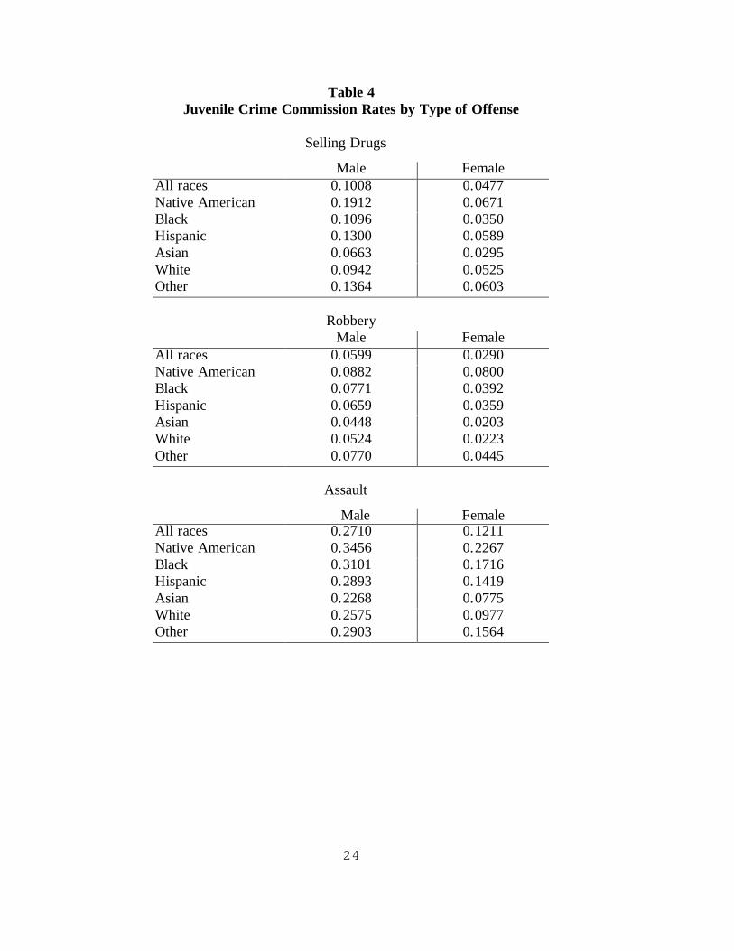
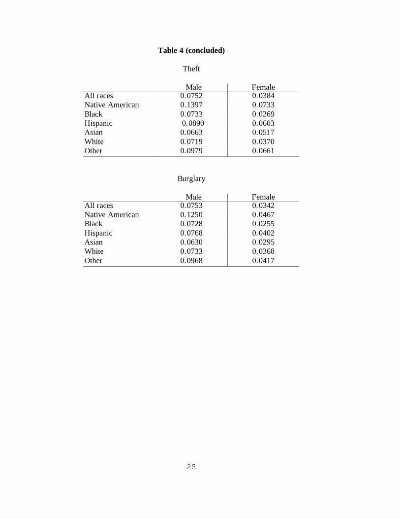
Table 4 displays the prevalence of different offenses by race and gender. Regarding

selling drugs, Asians have the lowest commission rate with 6.6 percent for males and less

than 3 percent for females. In contrast, almost one out of five Native American male

adolescents sold drugs at least once during the past year. The participation rates for males

range from 4 to 9 percent for robbery, 7 to 14 percent for theft, and 6 to 12.5 percent for

burglary among races. The rates for assault range from 23 percent to 35 percent. Native

American juveniles have the highest crime rates in all crime categories, and Asian

juveniles have the lowest crime rates.

It has been recognized that males commit more criminal offenses than females

(Gottfredson and Hirshi 1990, Henggeler 1989, Horwitz and White 1987). Consistent

with previous reports, our data set reveals that female juveniles offend at about half the

rate of their male counterparts. Criminologists and sociologists have developed a number

of theories to explain the contrast in criminal behavior between the genders. It has been

argued that gender differences in delinquent behavior can be attributed to differential

supervision of families for their sons and daughters (e.g. Hagan, Simpson and Gillis

1979), or to the difference in self-control between the sexes (Gottfredson and Hirschi

1990). The contrast in delinquent behavior can also be attributed to differences in risk

aversion (Powell and Ansic, 1997), discount rates ( Lau and Williams 1998), or the

motivation for security (Schnieder and Lopes, 1986). To account for these differences,

models are estimated separately for males and females.

Descriptive statistics presented in Table 5 suggest relationships between

juvenile crime, family structure, and family poverty as measured by welfare status.

Seventy-five percent of the adolescents who come from a two-parent household do not

7

engage in any crime; while the rate is 67 percent for those who come from one or no-

parent families. Similar differences in crime commission rates are observed for those who

are involved in one, two, three or four different types of crimes. The propensity to

commit a particular crime is also lower for those juveniles who come from two-parent

families. For example, 6.3 percent of the juveniles who have two parents sell drugs,

while the rate is 9.5 percent for those who have one or no parent. The same regularity is

observed for juveniles whose families are on welfare. The bottom two panels of Table 5

show that juveniles from families receiving public assistance have a higher propensity to

commit any given crime, and are, in general, more likely to engage in criminal behavior.

III. Juvenile Crime in the U.S.

Column I of Table 6 displays the population-weighted juvenile crime

participation rates for different offenses obtained from our data set. For comparison

purposes, column II presents the participation rates obtained from Wave 3 of the

National Youth Survey, conducted in 1979 (Ploeger 1997). Although the two surveys

are 15 years apart, the juvenile crime rates are of the same general magnitude.

However, in our data, which depict juvenile criminal behavior 1994-95, the

participation rates for burglary and theft are higher, whereas the participation rates for

selling drugs is lower.

Using the crime commission rates calculated from our data and employing

population weights, we estimated the number of juveniles who committed different

crimes in the U.S. in 1994. The results, which are reported in column III of Table 6,

indicate that in 1994 1.2 million juveniles sold drugs, and almost 3.3 million juveniles

assaulted someone. Eight-hundred and sixty-thousand juveniles were involved in theft,

866,000 committed burglary, and 725,000 committed robbery. Because the data set also

contains information on the frequency of these offenses, we are able to calculate the total

number of crimes committed by juveniles in each category. If the respondent indicated

that he/she committed 1 to 2 offenses it is converted into 1.5 offenses. A report of 3 to 4

offenses is converted in 3.5 offenses; and if the respondent indicated that an offense is

committed 5 or more times, it is converted into 5.5 crimes. Using this algorithm, we

8

calculated the total offenses committed for each crime, which is reported in column IV.

There were 3.7 million drug sales by juveniles, and 7 million assaults. They committed a

total of 1.7 million robberies, 2 million burglaries and 2 million thefts.

The above numbers can be compared to information obtained from official crime

statistics. The Uniform Crime Reports (UCR) of the FBI relies on information compiled

by local law enforcement agencies. The National Crime Victimization Survey (NCVS)

of the Bureau of Justice Statistics gathers crime information by asking a nationally

representative sample of persons ages 12 and above about crimes in which they were the

victim. To obtain an estimate of juvenile crime in 1994 using official data, we followed

the algorithm used by Levitt (1998), calculating the number of juvenile crimes as

[JARR/TARR]*CRIME, where JARR is juvenile arrests, TARR is total arrests, and

CRIME is the number of total crimes committed in a given category. This algorithm

assumes that the proportion of juvenile arrests for a given type of crime is a good proxy

for the proportion of juveniles actually committing that type of crime. The arrest

information is obtained from the UCR, and the crime information is obtained from the

NCVS. Column V displays the number of juvenile crimes suggested by the algorithm.

Table 6 indicates that the imputation of juvenile crime using official arrest and

victimization data may overstate the extent of juvenile theft, and understate juvenile

assault and robbery.

IV. Basic Methodology and Results

Following the seminal work of Becker (1968) and its extensions by Ehrlich

(1973) and Block and Heineke (1975), we postulate that participation in criminal

activity is the result of an optimizing individual’s reaction to incentives. More precisely,

individuals engage in criminal activities depending upon the expected payoffs of the

criminal activity, the return to legal labor market activity, tastes, and the costs of

criminal activity, such as those associated with apprehension, conviction and

punishment. Following this framework, the empirical implementation is depicted as

follows:

9

(1) Cij = αj+Xij’βj+ Yij’γj +Zij’δj+ εij,

where Cij is a dichotomous variable which takes the value of one if individual i

participated in crime j, and zero otherwise. The vector X consists of individual

characteristics, such as age, race, ethnicity and religion. It also includes family

characteristics, such as parent education, family’s welfare participation and family

structure. The vector Y includes neighborhood characteristics, such as the county

poverty as measured by per capita local welfare spending, and other county

characteristics such as the population density and the proportion of population who are

black or Hispanic. Following Levitt (1998), we also include the total number of

crimes in the county per 100,000 population to control for the impact of omitted

factors that may influence juvenile crime.

Legal employment opportunities are measured by the unemployment rate in

the county. Although theoretically well-defined, the relationship between crime and

unemployment is found to be modest in economics literature (Freeman 1983).

Criminology literature includes conflicting results on unemployment-crime relationship

(Kapuscinski, Braithwaite and Chapman, 1998).

The data set does not contain a measure of wages for juveniles. This is not a

drawback because all individuals in the data set are high school students, and

therefore, controlling for age, there should be little variation in wages. On the other

hand, employment opportunities may vary significantly, and, in fact, area

unemployment has been shown to have a sizable effect on the employment probability

of young adults (Freeman and Rodgers 1999). The local unemployment in the data set

pertains to 1990, while most of the crime information for juveniles pertains to 1994.

To the extent that there is hysteresis in unemployment, this is not a major issue. Also,

it should be noted that Freeman and Rodgers (1999) find that past unemployment has

an independent effect on the current labor market outcomes of young workers.

The vector Z consists of variables that measure sanctions at the county level.

They are the arrest rates per violent crime, the arrest rate for the property crimes and per

capita local government spending on police protection. Our arrest variables pertain to the

10

total arrest rates for violent and property crimes, instead of juvenile arrests, reducing the

likelihood of reverse causality from individual criminal activity to total arrest rates.

Perhaps of greater importance, the arrest variables correspond to 1993, while criminal

activity pertains to 1994-95. Thus, an increase in the arrest rates in 1993 is assumed to

impact juvenile delinquent behavior approximately one year later, but an increase in

juvenile crime cannot change the arrest rates in the previous year. Police expenditures

are measured in 1987, seven years prior to the behavior we are investigating.

Admittedly, this is a long lag, even in the presence of high serial correlation in police

spending. Further, this measure of police spending not only includes expenditures on

police protection and other crime prevention activities, but also activities that have little

or no impact on crime, such as traffic safety and vehicular inspection. These issues may

make it difficult to detect a significant relationship between crime and police spending,

but this is the only police expenditure available in the data. Tests for the exogeneity of

the deterrence measures are carried out, and are explained below.

Tables 7A-7E present the results from probit models for criminal participation

for males for five different crimes. The entries are the marginal effects, and the

associated standard errors are reported in parentheses. Huber corrected standard errors

are reported to account for within-county correlation between error terms.

Selling Drugs

Table 7A presents estimates of Equation (1) for selling drugs. All else equal,

blacks have almost a 2 percent higher propensity to sell drugs. Asians are 3 percent less

likely to sell drugs, and Native Americans are 10 percent more likely. Hispanic origin is

associated with an increase in this probability of almost 3 percent. Age also has a

positive impact on the likelihood of selling drugs. All else equal, adolescents who are 14

years old have almost a 10 percent higher probability of selling drugs in comparison to

individuals in 12-to-13 year age group (the omitted category). Juveniles who are 15, 16

and 17 years of age are 13 percent, 16 percent and 18 percent more likely, respectively,

to sell drugs.

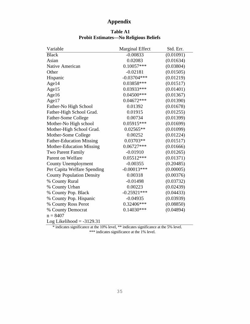
Religious beliefs influence the selling of drugs. Adolescents who identified

11

themselves as Born Again Christians are 3 percent less likely to sell drugs. Juveniles

who identified themselves as having no religious beliefs are 3 percent more likely to

engage in the selling of drugs. This result is consistent with results reported by Freeman

(1986), who showed that churchgoing affects the allocation of time, school attendance,

work activity and deviant behavior, and helps youths escape from inner-city poverty. It

can be argued that the link between religion and criminal activity is not causal, but

unobservable characteristics of juveniles which affect their religious beliefs also influence

their criminal behavior. Following Freeman (1986) we postulate that if religious beliefs

are endogenous, rather than exogenous, the pattern of the relationship between

independent variables and crime would be similar to the ones in an equation explaining

religious belief. A probit model in which a dichotomous variable takes the value of one

if the juvenile has no religion, and zero otherwise is estimated as a function of the same

background variables in our crime equations. The results, which are reported in the

Appendix (Table A1) show a different pattern of results than found from the crime

regressions. For example, being of Hispanic origin lowers the probability of having no

religious beliefs. Unemployment and two-parent household have no impact on religion,

but the proportion of blacks, the proportion who voted Democratic or voted for Ross

Perot in the county affect religious beliefs. Low-educated mothers make it less likely for

male juveniles to have religious beliefs. These results, which are similar to those

reported by Freeman (1986) suggest a causal mechanism from religion to juvenile

criminal behavior.

If the mother attended, but did not graduate from college, this increases the

probability of selling drugs in comparison to cases where the mother has a college

degree. The presence of two parents in the family decreases the probability of selling

drugs by 3 percent in comparison to single or no parent families. The coefficient of the

variable measuring family poverty is positive but statistically insignificant.

The characteristics of the neighborhood also have an impact on the behavior of

the juveniles. Per capita local welfare spending in the county has a positive impact on the

propensity to sell drugs. If increased poverty, represented by high welfare spending, is

associated with a reduced demand for drugs because of a negative income effect, the

12

corresponding reduction in price and transaction in drugs may reduce the producer

surplus in the market. Under this scenario, a hard-core, professional drug seller may

leave the market, creating room for the entry of juvenile sellers.

The unemployment rate is positive and significant, suggesting that living in areas

with few employment opportunities encourages male juveniles to earn illegal incomes by

selling drugs. The population density of the county has a negative effect on selling drugs,

indicating that, all else equal, living in the low density areas increases the propensity to

sell drugs for juveniles. The proportion of Hispanics in the county negatively impacts the

propensity to sell drugs, and the probability goes up with the proportion of population

who voted for Ross Perot and Democratic in 1992 presidential elections.

Per capita police spending and the arrest rate for property crimes in the county

have no impact on the decision to sell drugs, but as predicted by economic model of

crime, an increase in the arrest rate for violent crimes in the county decreases the

probability of selling drugs for juveniles. Specifically, an additional arrest per violent

crime reduces the probability of selling drugs for juvenile males by 4 percent.

Assault

Table 7B presents the estimated probit models for assault for juvenile males.

The only race effect is for blacks: black male adolescents have almost 4 percent higher

probability of assaulting someone, keeping constant personal, family, and county

characteristics, and deterrence measures. The coefficients of AGE14 is positive and

statistically significant, while the coefficients of AGE15, AGE16 and AGE17 are not

different from zero. This suggests that the propensity to assault for juvenile males peaks

at age 14. Being a Born-Again Christian lowers the probability of committing assault by

3.7 percent, while being a Catholic lowers it by 3.1 percent.

Mother’s education has no impact on the offspring’s propensity to assault, but

adolescent males are 8 percent more likely to assault if their father has only a high school

education, and 5 percent more likely to assault if the father attended, but not finished

college. Children from two-parent families have 4 percent lower probability to assault,

all else being the same.

13

Poverty in the county is positively related to the likelihood to commit assault,

which is consistent with the finding of Corman and Mocan (forthcoming), who report a

positive relationship between poverty and murders in New York City. Table 7B also

presents additional evidence to support the deterrence hypothesis. An additional arrest

per violent crime is associated with a reduction in the probability of assault for juvenile

males by 6 percent.

Robbery

Table 7C presents the results for robbery. Black male juveniles have 1.5 percent

higher probability to commit robbery than whites. There are no statistical differences

between estimated age coefficients. This suggests that 14-to-17 year olds are more likely

to commit robbery than younger children, but otherwise there are no significant

differences by age. Coming from a two-parent family has no impact on committing

robbery, but if a parent receives public assistance the juvenile’s propensity to commit

robbery is 2.5 percent higher.

Unemployment and poverty in the county have positive impacts, demonstrating the

importance of economic conditions. For example, a one percentage point increase in the

unemployment rate is associated with a three percent increase in the probability of

committing a robbery. However, the results from this regression provide no evidence of

a deterrence effect. The estimated coefficients of the arrest and police spending variables

are neither individually, nor jointly significant. These results suggest that family and

neighborhood poverty are better predictors of the propensity to committing robbery than

deterrence variables.

Burglary

Table 7D presents the results for burglary. Native American male juveniles and

juveniles belonging to the “other race” category have a higher propensity to burglarize.

As was the case for robbery, the hypothesis of the equality of the age coefficients cannot

be rejected. Having no religious beliefs increases the probability to commit burglary by

4 percent. County characteristics, including unemployment and poverty have no impact

14

on burglary, but family poverty has a positive impact: if the family is on welfare, this

increases the child’s propensity to commit burglary by 3 percent. Arrest rates and police

force do not have an impact on burglaries committed by male juveniles.

Theft

Table 7E displays the results for theft. All else equal, Native Americans have a

higher propensity to commit theft. Adolescents who are 14 years of age are more likely

to steal in comparison to younger ones, and adolescents who are 15-17 are more likely to

steal in comparison to 14 year olds. Having no religious beliefs increases the propensity

to steal by 4 percent. If the family is on welfare, the probability to steal is 4 percent

higher.

Although the deterrence variables are lagged, their potential endogeneity cannot be

ruled out. Following Tauchen, Witte and Griesinger (1994) we tested the endogeneity of

per capita police spending and arrest rates. Using the Rivers and Vuong test (1988), we

instrumented our deterrence measures with county government spending on education

and health, and state spending on education, health, and welfare. In the first stage

regressions the five instruments were jointly extremely significant (p=0.000), and in no

case could we reject the null hypothesis of the exogeneity of the deterrence variables.

All the models were also estimated for females. The results revealed interesting

differences between male and female juvenile criminal behavior. Table A2 in the

appendix summarizes the results for females. In contrast to the male results, the

propensity to sell drugs is lower for black female juveniles as compared to white females.

Parental education has a more pronounced impact on female delinquency than was the

case for males. Similarly, local area characteristics such as population density,

proportion of population in rural areas and proportion Hispanic are more important

determinants of female criminal activity. There is also a difference in the age-crime

relationship. With the exception of selling drugs, female juvenile criminal activity peaks

before age 17 for females. Violent crime arrests deter theft and drug sales of females.

Finally, we estimated ordered probit models for both genders. As reported in

15

Table 2, criminal activity is classified into four different frequency categories for each

offense: zero offenses, one to two offenses, three to four offenses, and five or more

offenses. The results of these ordered probits are consistent with the participation

regression results, and the results for males are presented in the Appendix.

V. Summary and Simulations

Table 8 summarizes the results reported in Tables 7A-7E for selected variables.

Some of the county characteristics and variables that were consistently statistically

insignificant are not included. The variables in the upper section of Table 8 can be

thought of as non-policy variables. They are race, age and religion of the juvenile male.

It is not clear why race is a determinant of criminal activity after controlling for a host of

personal, family and neighborhood characteristics. It is possible that race is capturing

some effect not measured by the variables in the model. For example, although all of the

individuals in our sample are enrolled in high school, it is possible that the quality of

education is correlated with race.

The variables in the lower section of Table 8 can be manipulated by policy

makers. Among them are parental education, family structure, family poverty,

unemployment and poverty in the county of residence, and the arrest rate for violent

crimes in the county. Selling drugs and assaults are sensitive to increases in violent crime

arrests. Family poverty, measured by family welfare status has a positive impact on

juveniles’ involvement in robbery, burglary, and theft. County poverty, measured by per

capita local welfare spending, has a positive impact on selling drugs, assault, and

robbery. Local unemployment affects the selling of drugs and robbery.

The presence of two parents in the family lowers juvenile males’ participation in

assault and selling drugs, perhaps a reflection of parental supervision. Glaeser, Sacerdote

and Scheinkman (1996) explore the influence of social interactions on crime. They find

higher levels of social interactions in cities with more female-headed households, and

suggest that social interactions among criminals are higher if the family units are not

intact. Our results can also be seen as providing support for the social interaction

hypothesis. Specifically, the negative relationship between two-parent households and

16

juvenile crime may be due to closer supervision of children in these households.

The effects summarized in Table 8 are often substantial in magnitude. Moving

from a one- or no-parent household to a two-parent household reduces the probability of

selling drugs by 2.7 percent and the probability of assault by 3.8 percent (Table 9). If the

family leaves the welfare rolls, this reduces the propensity to commit property crimes for

the juvenile male. More precisely, the probability to commit robbery, burglary and theft

goes down by 2.5 percent, 3 percent, and 4.4 percent, respectively. As Table 9

demonstrates, a two percentage point decrease in the unemployment rate lowers the

probability of selling drugs by 0.8 percent, and the probability of committing robbery by

0.6 percent. A 50 percent increase in the arrest rate for violent crimes reduces the

probability of selling drugs by 1.1 percent, and the probability of assault by 1.4 percent.

A natural question to ask is how consistent these results are with recent trends in

juvenile crime. Time-series data on juvenile crime are not available. Following Levitt

(1998), juvenile crime can be imputed by using the Uniform Crime Reports of the FBI

and the National Crime Victimization Survey data. Using the algorithm described

earlier, we calculated that in 1989 there were a total of 4.7 million crimes committed by

juveniles. This is the sum of juvenile robberies, assaults, burglaries and thefts. Total

juvenile crime increased to 7.8 million by 1993: an increase of 3.1 million offenses.

During the same time period the arrest rates and police spending increased as well.

However, these increases are potentially endogenous; they may have been determined by

increases in crime rate. On the other hand, there were two changes during the same

period which can be considered exogenous. The aggregate unemployment rate increased

by 1.4 percentage points (from 5.5 percent to 6.9 percent) and the AFDC caseload also

increased during the same period (U.S. House Committee on Ways and Means 1998) .

(Specifically, the number of AFDC children increased by 1 million between 1988 and

1993). Using these numbers and the estimated parameters presented in the paper, a

rough calculation indicates that the increase in unemployment and family poverty can

explain approximately 14 percent of the increase in juvenile crime between 1989 and

1993. By 1996, the unemployment rate went down to 5.4 percent, and the number of

children in poverty decreased by 1.1 million. The total number of juvenile crimes went

17

down to 7.2 million offenses. The decline in unemployment and poverty explain 28

percent of the decrease in juvenile crime during this period.

VI. Conclusion

This is the first paper to test the economic model of crime for juveniles using

micro data. It uses a nationally representative sample of 16,478 high school children

surveyed in 1995. The data set allows for a portrayal of the extent of juvenile crime, as

well as an investigation of race and gender differences in criminal behavior and the

impacts of economic and deterrence variables.

In 1994 approximately 7 million juveniles (one-quarter of adolescents in 11-17

age group) were involved in at least one type of criminal act. One million and two

hundred thousand juveniles sold drugs, 3.3 million assaulted someone, 725,000 juveniles

committed robbery, 866,000 committed burglary and 860,000 stole something worth

more than $50, and they committed a total of 16.5 million offenses in 1994. There are

substantial differences between races in crime commission rates. For example, 46

percent of Native American juvenile males committed at least one crime, while the rates

are 40 percent for black males, 35 percent for white males, 31 percent for Asian males.

Almost one out of five Native American males sold drugs. The corresponding rates are

approximately one-in-ten for blacks and whites, and one-in-fifteen for Asian males. The

crime commission rates of females are roughly half that of males.

We find that juveniles respond to incentives as predicted by economic theory.

An increase in violent crime arrests reduces the probability of selling drugs and assaulting

someone for males, and reduces the probability of selling drugs and stealing for females.

An increase in local unemployment increases the propensity to commit crimes, as does

local poverty. Similarly, family poverty increases the probability to commit robbery,

burglary and theft for males, and assault and burglary for females. Local characteristics

are more important for females than males.

Racial differences persist even after controlling for personal and family

characteristics and deterrence measures. For example, all else equal, in comparison to

whites, black male juveniles are more likely to sell drugs, commit robbery, and commit

18

assault. It is not clear why racial differences exist after controlling for personal, family,

county characteristics, the unemployment rate and deterrence measures. One explanation

is that race may act as a proxy for unobservable neighborhood or school characteristics.

Education of the parents has a more pronounced impact on female juvenile

criminal activity than that of males. This is especially true for mother’s education, where

the daughters of college educated mothers have lower propensity to sell drugs, assault,

rob or steal. Religious beliefs impact the propensity to commit crime as does the family

structure. Male juveniles who come from two-parent families are less likely to assault

and sell drugs, while juvenile females from two-parent families are less likely to sell

drugs, assault and rob, which suggests that family supervision has an impact on

delinquent behavior.

Simulations show that the increase in unemployment and family poverty can

explain approximately 14 percent of the increase in juvenile crime between 1989 and

1993, and the decline in the unemployment rate and the number of children in poverty

explain 28 percent of the decrease in juvenile crime between 1993 and 1996.

These results, taken together, show that the notion of “new breed of young

predators who do not respond to incentives” does not have empirical support. Juveniles

do respond to incentives and sanctions. Employment opportunities, increased family

income and more strict deterrence are effective tools to reduce juvenile crime.

19

Table 1Descriptive Statistics

Variable Definition

From: National Longitudinal Study of Adolescent Health

Female 0.51(0.50)

Dichotomous variable equal to 1 if female, 0if male.

Age 14 0.16(0.37)

Dichotomous variable equal to 1 ifrespondent was 14 years of age at the time ofthe interview, equal to 0 otherwise.

Age 15 0.21(0.41)


Age 16 0.24(0.42)

Dichotomous variable equal to 1 if therespondent was 16 years of age at the time ofthe interview, equal to 0 otherwise.

Age 17 0.23(0.42)


Hispanic 0.17(0.37)

Dichotomous variable equal to 1 if therespondent said they were of Hispanic orLatino origin, equal to 0 otherwise.

Black 0.24(0.43)

Dichotomous variable equal to 1 if therespondent said they were black or AfricanAmerican, equal to zero otherwise.

Asian 0.07(0.25)

Dichotomous variable equal to 1 if therespondent said they were Asian or PacificIslander, equal to 0 otherwise.

Native American 0.02(0.13)

Dichotomous variable equal to 1 if therespondent said they were Native Americanor American Indian, equal to 0 otherwise.

Other Race 0.09(0.28)

Dichotomous variable equal to 1 if therespondent said they belonged to anunspecified “other” race, equal to 0otherwise.

Father-No High School 0.10(0.30)

Dichotomous variable equal to 1 if residentfather did not graduate from high school,equal to 0 otherwise.

Father-High School Grad. 0.21(0.41)

Dichotomous variable equal to 1 if residentfather graduated from high school orreceived a GED, equal to 0 otherwise.

20

Father-Some College 0.12(0.32)

Dichotomous variable equal to 1 if theresident father attended college but did notgraduate, equal to 0 otherwise.

Father-College Grad. 0.22(0.41)

Dichotomous variable equal to 1 if theresident father graduated from college, equalto 0 otherwise.

Father-Education Missing 0.35(0.48)

Dichotomous variable equal to 1 if there wasno resident father or if respondent did knowfather’s schooling, otherwise equal to 0.

Mother-No High School 0.14(0.35)

Dichotomous variable equal to 1 if residentmother did not graduate from high school,equal to 0 otherwise.

Mother-High School Grad. 0.32(0.47)

Dichotomous variable equal to 1 if residentmother graduated from high school orreceived a GED, equal to 0 otherwise.

Mother-Some College 0.18(0.39)

Dichotomous variable equal to 1 if theresident mother attended college but did notgraduate, equal to 0 otherwise.

Mother-College Graduate 0.26(0.44)

Dichotomous variable equal to 1 if theresident mother graduated from college,equal to 0 otherwise.

Mother-Education Missing 0.10(0.30)

Dichotomous variable equal to 1 if there wasno resident mother or if respondent did knowmother’s schooling, otherwise equal to 0.

Two Parent Family 0.66(0.47)

Dichotomous variable equal to 1 ifrespondent lived with two parents, equal to 0otherwise.

Parent on Welfare 0.12(0.32)

Dichotomous variable equal to 1 if eitherresident parent received public assistance,and equal to 0 otherwise.

Born Again Christian 0.26(0.44)

Dichotomous variable equal to 1 ifrespondents said they were Born AgainChristian, and equal to 0 otherwise.

Catholic 0.26(0.44)

Dichotomous variable equal to 1 ifrespondents said they were Catholic, andequal to 0 otherwise.

No Religion 0.12(0.32)

Dichotomous variable equal to 1 ifrespondents said they had no religiousbeliefs, and equal to 0 otherwise.

Baptist 0.22(0.41)

Dichotomous variable equal to 1 ifrespondent said they were Baptist, and equalto 0 otherwise.

21

From: 1990 Census of Population and Housing

County Unemployment 0.07(0.02)

Percent unemployed of the civilian laborforce in the county of residence.

% County Rural 0.23(0.27)

Proportion of the county population living ina rural area.

% County Urban 0.66(0.39)

Proportion of the county population living inan urban area.

County Population Density 0.58(1.53)

Persons per square kilometer in the county ofresidence.

% County Pop. Black 0.15(0.14)

Proportion of the county population black.

% County Prop. Hispanic 0.10(0.14)

Proportion of the county populationHispanic.

From: USA Counties (Bureau of the Census, 1994)

Per Capita Police Spending 90.55(45.18)

Per capita local government direct generalexpenditures on police protection in thecounty of residence, 1987.

Per Capita WelfareSpending

77.61(103.77)

Per capita local government direct generalexpenditures on public welfare in the countyof residence, 1987.

% Democrat 0.44(0.10)

Proportion voting Democratic in the 1992presidential elections in the county ofresidence.

% Ross Perot 0.18(0.06)

Proportion voting for Perot in the 1992presidential elections in the county ofresidence.

From: Uniform Crime Reports (FBI, 1994)

County Crime Rate 5998.48(2859.49)

The number crimes in the county per100,000 persons.

Arrests per Violent Crime 0.46(0.29)

Total violent crime arrests divided by thenumber of violent crimes in the county ofresidence, 1993.

Arrests per Property Crime 0.19(0.09)

Total property crime arrests divided by thenumber of property crimes in the county ofresidence, 1993.

n = 16,478

22

Table 2Descriptive Statistics for Juvenile Offenses

Variable Definition Mean Std. Dev.In the past 12 months did you . . .

Sold Drugs sell marijuana or other drugs? 0.073 0.261Sold Drugs_12 . . . 1 or 2 times 0.037 0.189Sold Drugs_34 . . . 3 or 4 times 0.011 0.103Sold Drugs_5+ . . . 5 or more times 0.026 0.158Assault hurt someone badly enough to need

bandages or care from a doctor or nurse? 0.194 0.396Assault_12 . . . 1 or 2 times 0.148 0.355Assault_34 . . . 3 or 4 times 0.024 0.154Assault_5+ . . . 5 or more times 0.022 0.147Robbery use or threaten to use a weapon to get

something from someone? 0.044 0.205Robbery_12 . . . 1 or 2 times 0.032 0.177Robbery_34 . . . 3 or 4 times 0.006 0.079Robbery_5+ . . . 5 or more times 0.006 0.074Burglary go into a house to steal something? 0.054 0.227Burglary_12 . . . 1 or 2 times 0.038 0.192Burglary_34 . . . 3 or 4 times 0.007 0.083Burglary_5+ . . . 5 or more times 0.009 0.094Theft steal something worth more than $50? 0.056 0.231Theft_12 . . . 1 or 2 times 0.038 0.191Theft_34 . . . 3 or 4 times 0.008 0.091Theft_5+ . . . 5 or more times 0.010 0.100

23

Table 3

Proportion of Juveniles Who Committed

at Least One Crime

Male Female

All races 0.361 0.190

White 0.348 0.169

Black 0.401 0.229

Native American 0.463 0.295

Asian 0.310 0.146

Other 0.381 0.252

Juvenile Crime Commission Rates

Crimes Males Females

None 0.639 0.810

One type of Crime 0.235 0.138

2 Different Crimes 0.071 0.034




24

Table 4Juvenile Crime Commission Rates by Type of Offense

Selling Drugs

Male FemaleAll races 0.1008 0.0477Native American 0.1912 0.0671Black 0.1096 0.0350Hispanic 0.1300 0.0589Asian 0.0663 0.0295White 0.0942 0.0525Other 0.1364 0.0603

RobberyMale Female

All races 0.0599 0.0290Native American 0.0882 0.0800Black 0.0771 0.0392Hispanic 0.0659 0.0359Asian 0.0448 0.0203White 0.0524 0.0223Other 0.0770 0.0445

Assault


25

Table 4 (concluded)

Theft


Burglary


26

Table 5Juvenile Crime by Family Structure and Poverty

Number of Different Crimes(Selling Drugs+Assault+Robbery+Burglary+Theft)

Two ParentHousehold

0 1 2 3 4 5+

No 67.3 21.1 6.6 2.9 1.4 0.8Yes 75.3 17.2 4.6 1.7 0.7 0.6

Two ParentHousehold

SellingDrugs

Assault Robbery Burglary Theft

No 9.5 23.6 5.7 6.6 7.1Yes 6.3 17.4 3.7 4.9 4.9

Number of Different Crimes(Selling Drugs+Assault+Robbery+Burglary+Theft)

Parent(s) onWelfare

0 1 2 3 4 5+

No 73.6 18.0 5.0 1.9 0.9 * 0.6Yes 65.5 22.1 6.8 3.5 1.0 * 1.1

Parent(s) onWelfare

SellingDrugs


No 7.2 18.6 4.2 5.2 5.3Yes 8.4 25.3 6.3 7.5 8.3

* indicates that the rates are not statistically different from each other.

27

Table 6Juvenile Criminal Activity

Offense

(I)JuvenileCrimeRate in

Our data(weighted)

(II)Juvenile

Crime RateNYS 1976

(Ploeger 1997)

(III)Number of

JuvenileParticipants

(IV)Number ofOffenses

Committed byJuveniles

(V)Imputed

Number ofJuvenile

Offenses fromOfficialSources

Selling Drugs 0.070 0.104 1,210,000 3,748,000 --Assault 0.190 0.042, 0.330 * 3,278,000 7,033,000 1,488,000Robbery 0.042 -- 725,000 1,680,000 411,501Burglary 0.050 0.024 866,000 2,057,000 2,106,000Theft 0.050 0.026 860,000 2,049,000 3,891,000

* The entries in this cell represent the offense rates for “attacking someone,” and“hitting students,” respectively.

28

Table 7AThe Determinants of Selling Drugs—Juvenile Males

Variable Marginal Effect Std. Err.Black 0.01839** (0.00977)Asian -0.03157*** (0.00884)Native American 0.10180*** (0.03635)Other Race 0.01810 (0.01252)Hispanic 0.02605** (0.01261)Age14 0.09702*** (0.02051)Age15 0.13029*** (0.02063)Age16 0.15750*** (0.01799)Age17 0.17712*** (0.02011)Born Again Christian -0.02981*** (0.00762)Catholic -0.00927 (0.00896)Baptist -0.00289 (0.01005)No Religion 0.02843*** (0.01130)Father-No High School 0.00845 (0.01528)Father-High School Grad. 0.00235 (0.01105)Father-Some College 0.01787 (0.01611)Mother-No High School 0.00555 (0.01310)Mother-High School Grad. 0.00789 (0.00956)Mother-Some College 0.02555** (0.01267)Father-Education Missing 0.01016 (0.01419)Mother-Education Missing 0.02167* (0.01224)Two Parent Family -0.02709** (0.01292)Parent on Welfare 0.00852 (0.00914)County Unemployment 0.35624* (0.19126)Per Capita Welfare Spending 0.00011* (0.00006)County Population Density -0.01014*** (0.00257)% County Rural -0.06481 (0.04192)% County Urban -0.01772 (0.02930)% County Pop. Black -0.08390 (0.05267)% County Pop. Hispanic -0.15917*** (0.04453)% Ross Perot 0.22794** (0.09691)% Democrat 0.14380*** (0.04685)County Crime Rate 0.0000001 (0.000002)Per Capita Police Spending 0.00015 (0.00021)Arrests Per Property Crime 0.06246 (0.05799)Arrests Per Violent Crime -0.04229** (0.01679)n = 8026Log Likelihood = -2466.37

The standard errors are Huber corrected. * indicates significance at the 10% level, ** indicates significance atthe 5% level, *** indicates significance at the 1% level.

29

Table 7BThe Determinants of Assault—Juvenile Males

Variable Marginal Effect Std. Err.Black 0.03702** (0.01790)Asian -0.01893 (0.02745)Native American 0.06494 (0.04340)Other Race 0.00391 (0.01870)Hispanic 0.01158 (0.01968)Age14 0.03476* (0.02155)Age15 0.02951 (0.02017)Age16 0.02473 (0.01725)Age17 0.01290 (0.01578)Born Again Christian -0.03667** (0.01432)Catholic -0.03135* (0.01830)Baptist -0.00304 (0.01384)No Religion 0.01971 (0.01891)Father-No High School 0.03350 (0.02603)Father-High School Grad. 0.07768*** (0.01892)Father-Some College 0.04902** (0.02138)Mother-No High School 0.02355 (0.02396)Mother-High School Grad. 0.01095 (0.01781)Mother-Some College 0.00786 (0.01540)Father-Education Missing 0.06205*** (0.02101)Mother-Education Missing 0.00655 (0.02608)Two Parent Family -0.03843** (0.01741)Parent on Welfare 0.02432 (0.01674)County Unemployment 0.31657 (0.28663)Per Capita Welfare Spending 0.00020** (0.00010)County Population Density -0.00192 (0.00386)% County Rural 0.04521 (0.06638)% County Urban 0.04919 (0.03784)% County Pop. Black 0.09828 (0.07018)% County Pop. Hispanic 0.00079 (0.06097)% Ross Perot 0.33295** (0.13256)% Democrat -0.09326 (0.07282)County Crime Rate -0.000006 (0.000003)Per Capita Police Spending 0.00005 (0.00030)Arrests Per Property Crime -0.03700 (0.09170)Arrests Per Violent Crime -0.06265* (0.03312)n = 8031Log Likelihood = -4617.04

The standard errors are Huber corrected. * indicates significance at the 10% level, ** indicates significanceat the 5% level, *** indicates significance at the 1% level.

30

Table 7CThe Determinants of Robbery—Juvenile Males

Variable Marginal Effect Std. Err.Black 0.01500** (0.00758)Asian -0.00555 (0.00943)Native American 0.03325 (0.02619)Other Race 0.01883 (0.01364)Hispanic -0.00233 (0.00861)Age14 0.02968** (0.01356)Age15 0.03353*** (0.01158)Age16 0.04174*** (0.01164)Age17 0.03030*** (0.01189)Born Again Christian -0.00589 (0.00639)Catholic -0.01462** (0.00643)Baptist -0.00782 (0.00744)No Religion 0.01074 (0.00871)Father-No High School 0.00823 (0.01273)Father-High School Grad. -0.000004 (0.00725)Father-Some College 0.01314 (0.01005)Mother-No High School 0.01168 (0.01202)Mother-High School Grad. -0.00057 (0.00712)Mother-Some College -0.00555 (0.00764)Father-Education Missing 0.02154** (0.00975)Mother-Education Missing 0.01341 (0.00980)Two Parent Family 0.00024 (0.00866)Parent on Welfare 0.02512*** (0.00879)County Unemployment 0.28533** (0.13106)Per Capita Welfare Spending 0.00010** (0.00004)County Population Density -0.00357** (0.00154)% County Rural -0.03658 (0.02405)% County Urban 0.00830 (0.01545)% County Pop. Black 0.01161 (0.03249)% County Pop. Hispanic -0.04935* (0.03034)% Ross Perot -0.00278 (0.06742)% Democrat -0.02659 (0.03678)County Crime Rate -0.000001 (0.000002)Per Capita Police Spending -0.00011 (0.00018)Arrests Per Property Crime -0.00349 (0.03951)Arrests Per Violent Crime -0.00616 (0.01721)n = 8041Log Likelihood = -1778.09


31

Table 7DThe Determinants of Burglary—Juvenile Males

Variable Marginal Effect Std. Err.Black 0.00322 (0.01007)Asian -0.00864 (0.01006)Native American 0.04560* (0.03164)Other Race 0.03628*** (0.01507)Hispanic -0.01709* (0.00906)Age14 0.02752*** (0.01091)Age15 0.03773*** (0.01284)Age16 0.03452*** (0.01022)Age17 0.02141** (0.01037)Born Again Christian 0.00153 (0.00738)Catholic 0.00278 (0.00808)Baptist -0.00449 (0.00848)No Religion 0.03723*** (0.01151)Father-No High School 0.00028 (0.01376)Father-High School Grad. 0.00684 (0.00949)Father-Some College -0.00274 (0.01089)Mother-No High School -0.00773 (0.01010)Mother-High School Grad. -0.00515 (0.00860)Mother-Some College -0.01228 (0.00894)Father-Education Missing 0.02464** (0.01100)Mother-Education Missing 0.01831* (0.01011)Two Parent Family -0.00284 (0.00854)Parent on Welfare 0.03054*** (0.01114)County Unemployment -0.02519 (0.18942)Per Capita Welfare Spending 0.00005 (0.00007)County Population Density -0.00136 (0.00250)% County Rural -0.04753 (0.03384)% County Urban -0.00193 (0.02108)% County Pop. Black -0.03844 (0.04655)% County Pop. Hispanic 0.01929 (0.05871)% Ross Perot -0.00773 (0.07892)% Democrat -0.03303 (0.05111)County Crime Rate -0.0000007 (0.000003)Per Capita Police Spending -0.00024 (0.00019)Arrests Per Property Crime 0.06343 (0.04672)Arrests Per Violent Crime 0.00185 (0.01644)n = 8039Log Likelihood = -2118.96


32

Table 7EThe Determinants of Theft—Juvenile Males

Variable Marginal Effect Std. Err.Black 0.00123 (0.00805)Asian -0.01363 (0.01095)Native American 0.04388* (0.02915)Other Race 0.01885 (0.01404)Hispanic -0.01540 (0.00967)Age14 0.02832** (0.01246)Age15 0.05187*** (0.01152)Age16 0.05149*** (0.01110)Age17 0.05348*** (0.01296)Born Again Christian -0.00373 (0.00742)Catholic -0.00058 (0.00718)Baptist -0.01313 (0.00776)No Religion 0.03853*** (0.01324)Father-No High School -0.01096 (0.01105)Father-High School Grad. 0.00334 (0.00953)Father-Some College 0.00867 (0.00852)Mother-No High School 0.01644 (0.01209)Mother-High School Grad. 0.01355* (0.00742)Mother-Some College 0.00789 (0.00911)Father-Education Missing 0.01684* (0.00980)Mother-Education Missing 0.04364*** (0.01482)Two Parent Family -0.00770 (0.00862)Parent on Welfare 0.04381*** (0.00951)County Unemployment 0.02270 (0.16824)Per Capita Welfare Spending 0.00005 (0.00004)County Population Density -0.00255 (0.00162)% County Rural -0.06739** (0.03002)% County Urban -0.01734 (0.01749)% County Pop. Black -0.03875 (0.04111)% County Pop. Hispanic 0.01724 (0.02437)% Ross Perot -0.00307 (0.06340)% Democrat -0.05479 (0.03929)County Crime Rate -0.00000005 (0.000002)Per Capita Police Spending 0.00001 (0.00015)Arrests Per Property Crime 0.07028 (0.04449)Arrests Per Violent Crime -0.01782 (0.01738)n = 8043Log Likelihood = -2081.80


33

Table 8Summary Results for Juvenile Males

SellingDrugs


VariableBlack + + +Native American + + +Asian --Other +Hispanic +Age 14 + + + + +Age 15 + + + + +Age 16 + + + + +Age 17 + + + + +Born Again Christian -- --Catholic -- --No Religion + + +Father High school +Father some College +Mother High school +Mother some College +Two Parent Family -- --Parent on Welfare + + +County Unemployment + +Per Capital WelfareSpending

+ + +

Arrests Per Violent Crime -- --

34

Table 9The Impact of Selected Determinants on Juvenile Offenses

SellingDrugs


Two Parent(67%)

A Switch To Two-ParentFamily -2.7% -3.8%

Parent on Welfare(12%)

Family Out of Welfare -2.5% -3.0% -4.4%

Unemployment(6.8%)

A Two Percentage PointDecline in UnemploymentRate

-0.8% -0.6%

Violent ArrestRate (46%)

A 50% Increase in ArrestRate -1.1% -1.4%

The numbers in parentheses in the first column are sample means for the correspondingvariable.

35

Table A1Probit Estimates—No Religious Beliefs

Variable Marginal Effect Std. Err.Black -0.00833 (0.01091)Asian 0.02083 (0.01634)Native American 0.10057*** (0.03804)Other -0.02181 (0.01505)Hispanic -0.03704*** (0.01219)Age14 0.03858*** (0.01517)Age15 0.03933*** (0.01401)Age16 0.04500*** (0.01367)Age17 0.04672*** (0.01390)Father-No High School 0.01392 (0.01678)Father-High School Grad. 0.01915 (0.01255)Father-Some College 0.00734 (0.01399)Mother-No High school 0.05915*** (0.01699)Mother-High School Grad. 0.02565** (0.01099)Mother-Some College 0.00252 (0.01224)Father-Education Missing 0.03703** (0.01517)Mother-Education Missing 0.06727*** (0.01666)Two Parent Family -0.01910 (0.01265)Parent on Welfare 0.05512*** (0.01371)County Unemployment -0.00355 (0.20485)Per Capita Welfare Spending -0.00013*** (0.00005)County Population Density 0.00318 (0.00376)% County Rural -0.01498 (0.03732)% County Urban 0.00223 (0.02439)% County Pop. Black -0.25921*** (0.04433)% County Pop. Hispanic -0.04935 (0.03939)% County Ross Perot 0.32406*** (0.08850)% County Democrat 0.14030*** (0.04894)n = 8407Log Likelihood = -3129.31

* indicates significance at the 10% level, ** indicates significance at the 5% level.*** indicates significance at the 1% level.

Appendix

36

Table A2Summary Results for Juvenile Females

SellingDrugs


Variable Female Female Female Female FemaleBlack -- +Native American + +Asian --Other Race + +Hispanic +Age14 + + +Age15 + +Age16 + -- -- +Age17 + -- --Born Again Christian -- --Baptist --CatholicNo Religion + + +Father-No High SchoolFather-High School Grad. + +Father-Some CollegeMother-No High School +Mother-High School Grad. + + + +Mother-Some College + +Two Parent Family -- -- --Parent on Welfare + +County Unemployment +County Population Density -- -- -- -- --% County Rural -- -- --% County Urban% County Pop. Black --% County Pop. Hispanic -- -- --% Ross Perot +% Democrat +County Crime Rate --Per Capita WelfareSpending

+ + +

Per Capita Police Spending

Arrests Per Violent Crime -- --Arrests Per Property Crime

37

Table A3The Determinants of Selling Drugs—Juvenile Males

(Ordered Probit)

Marginal Effects For . . .Variable Coefficient Selling Drugs

0 timesSelling Drugs1 or 2 times

Selling Drugs3 or 4 times

Selling Drugs5 or more

timesConstant -2.49577***

(0.27701)0.3912 -0.1601 -0.0602 -0.1709

Black 0.11740*(0.06159)

-0.0184 0.0075 0.0028 0.0080

Asian -0.22366**(0.09626)

0.0351 -0.0143 -0.0054 -0.0153

Native American 0.45851***(0.14496)

-0.0719 0.0294 0.0111 0.0314

Other Race 0.11445(0.08121)

-0.0179 0.0073 0.0028 0.0078

Hispanic 0.15294**(0.07197)

-0.0240 0.0098 0.0037 0.0105

Age14 0.48490***(0.09577)

-0.0760 0.0311 0.0117 0.0332

Age15 0.65234***(0.09043)

-0.1022 0.0418 0.0157 0.0447

Age16 0.77192***(0.08702)

-0.1210 0.0495 0.0186 0.0529

Age17 0.85167***(0.08704)

-0.1335 0.0546 0.0205 0.0583

Born Again Christian -0.19641***(0.05627)

0.0308 -0.0126 -0.0047 -0.0135

Catholic -0.04749(0.05602)

0.0074 -0.0030 -0.0011 -0.0033

Baptist -0.02077(0.06012)

0.0033 -0.0013 -0.0005 -0.0014

No Religion 0.19160***(0.06023)

-0.0300 0.0123 0.0046 0.0131


-0.0099 0.0041 0.0015 0.0043

Father-High SchoolGrad.

0.03461(0.06554)

-0.0054 0.0022 0.0008 0.0024


-0.0169 0.0069 0.0026 0.0074


-0.0044 0.0018 0.0007 0.0019

38

Table A3 (Concluded)Mother-High SchoolGrad.

0.04604(0.05728)

-0.0072 0.0030 0.0011 0.0032

Mother-Some College 0.14426**(0.06307)

-0.0226 0.0093 0.0035 0.0099

Father-EducationMissing

0.04621(0.08180)

-0.0072 0.0030 0.0011 0.0032

Mother-EducationMissing

0.12611*(0.07328)

-0.0198 0.0081 0.0030 0.0086

Two Parent Family -0.17856**(0.06939)

0.0280 -0.0115 -0.0043 -0.0122

Parent on Welfare 0.05139(0.06240)

-0.0081 0.0033 0.0012 0.0035

County Unemployment 2.19963*(1.20062)

-0.3448 0.1411 0.0530 0.1507


0.00076**(0.00032)

-0.0001 0 0 0.0001

County PopulationDensity

-0.06372***(0.01969)

0.0100 -0.0041 -0.0015 -0.0044

% County Rural -0.42538*(0.25232)

0.0667 -0.0273 -0.0103 -0.0291

% County Urban -0.10038(0.15879)

0.0157 -0.0064 -0.0024 -0.0069

% County Pop. Black -0.52061*(0.29742)

0.0816 -0.0334 -0.0125 -0.0357

% County Pop. Hispanic -1.00010***(0.24186)

0.1568 -0.0641 -0.0241 -0.0685

% Ross Perot 1.57530***(0.51886)

-0.2469 0.1010 0.0380 0.1079

% Democrat 0.95654***(0.29534)

-0.1499 0.0614 0.0231 0.0655


0 0 0 0

Per Capita PoliceSpending

0.00057(0.00112)

-0.0001 0 0 0

Arrests Per PropertyCrime

0.38452(0.36521)

-0.0603 0.0247 0.0093 0.0263

Arrests Per ViolentCrime

-0.28142**(0.11353)

0.0441 -0.0181 -0.0068 -0.0193

n = 8026Log Likelihood = -3285.65

* indicates significance at the 10% level, ** indicates significance at the 5% level,*** indicates significance at the 1% level.

39

Table A4The Determinants of Committing Assault—Juvenile Males

(Ordered Probit)

Marginal Effects For . . .Variable Coefficient Commit

Assault 0times

CommitAssault 1 or 2

times

CommitAssault 3 or 4

times

CommitAssault 5 ormore times

Constant -1.05128***(0.19969)

0.3464 -0.2048 -0.0623 -0.0792

Black 0.11161**(0.04414)

-0.0368 0.0217 0.0066 0.0084

Asian -0.04888(0.06456)

0.0161 -0.0095 -0.0029 -0.0037

Native American 0.20248*(0.10955)

-0.0667 0.0394 0.0120 0.0153

Other Race 0.02454(0.06404)

-0.0081 0.0048 0.0015 0.0018

Hispanic 0.04632(0.05680)

-0.0153 0.0090 0.0027 0.0035

Age14 0.08798*(0.05289)

-0.0290 0.0171 0.0052 0.0066

Age15 0.09634**(0.04893)

-0.0317 0.0188 0.0057 0.0073

Age16 0.08016*(0.04772)

-0.0264 0.0156 0.0048 0.0060

Age17 0.05188(0.04852)

-0.0171 0.0101 0.0031 0.0039

Born Again Christian -0.08152**(0.03967)

0.0269 -0.0159 -0.0048 -0.0061

Catholic -0.07204*(0.04119)

0.0237 -0.0140 -0.0043 -0.0054

Baptist -0.00295(0.04282)

0.0010 -0.0006 -0.0002 -0.0002

No Religion 0.11746**(0.04623)

-0.0387 0.0229 0.0070 0.0089

Father-No High School 0.12521**(0.06331)

-0.0413 0.0244 0.0074 0.0094


0.23292***(0.04879)

-0.0767 0.0454 0.0138 0.0176

Father-Some College 0.15002***(0.05443)

-0.0494 0.0292 0.0089 0.0113


-0.0204 0.0121 0.0037 0.0047

40


0.02710(0.04250)

-0.0089 0.0053 0.0016 0.0020


-0.0062 0.0037 0.0011 0.0014


0.18967***(0.05746)

-0.0625 0.0369 0.0112 0.0143


0.08008(0.05344)

-0.0264 0.0156 0.0047 0.0060

Two Parent Family -0.10973**(0.04975)

0.0362 -0.0214 -0.0065 -0.0083

Parent on Welfare 0.08806*(0.04604)

-0.0290 0.0172 0.0052 0.0066


-0.3589 0.2122 0.0646 0.0821


0.00062***(0.00022)

-0.0002 0.0001 0 0


-0.00704(0.01317)

0.0023 -0.0014 -0.0004 -0.0005

% County Rural 0.11712(0.16134)

-0.0386 0.0228 0.0069 0.0088

% County Urban 0.14283(0.10854)

-0.0471 0.0278 0.0085 0.0108

% County Pop. Black 0.32605(0.21065)

-0.1074 0.0635 0.0193 0.0246

% County Pop. Hispanic -0.13846(0.17684)

0.0456 -0.0270 -0.0082 -0.0104

% Ross Perot 1.07915***(0.37659)

-0.3555 0.2102 0.0640 0.0813

% Democrat -0.25071(0.21968)

0.0826 -0.0488 -0.0149 -0.0189

County Crime Rate -0.00001(0.00001)

0 0 0 0


0.00061(0.00084)

-0.0002 0.0001 0 0


-0.01725(0.25203)

0.0057 -0.0034 -0.0010 -0.0013


-0.18430**(0.08238)

0.0607 -0.0359 -0.0109 -0.0139



41

Table A5The Determinants of Committing Robbery—Juvenile Males

(Ordered Probit)


Robbery 0times

CommitRobbery 1 or

2 times

CommitRobbery 3 or

4 times

CommitRobbery 5 ormore times

Constant -1.81665***(0.33338)

0.2031 -0.1345 -0.0316 -0.0370

Black 0.14388**(0.06788)

-0.0161 0.0107 0.0025 0.0029

Asian -0.04722(0.10988)

0.0053 -0.0035 -0.0008 -0.0010


-0.0329 0.0218 0.0051 0.0060

Other Race 0.13575(0.09645)

-0.0152 0.0101 0.0024 0.0028

Hispanic 0.00237(0.09054)

-0.0003 0.0002 0 0

Age14 0.23549***(0.08907)

-0.0263 0.0174 0.0041 0.0048

Age15 0.25115***(0.08429)

-0.0281 0.0186 0.0044 0.0051

Age16 0.31404***(0.08082)

-0.0351 0.0233 0.0055 0.0064

Age17 0.23648***(0.08367)

-0.0264 0.0175 0.0041 0.0048

Born Again Christian -0.07547(0.06327)

0.0084 -0.0056 -0.0013 -0.0015

Catholic -0.13695**(0.06697)

0.0153 -0.0101 -0.0024 -0.0028

Baptist -0.05432(0.06702)

0.0061 -0.0040 -0.0009 -0.0011

No Religion 0.10214(0.07237)

-0.0114 0.0076 0.0018 0.0021


-0.0094 0.0062 0.0015 0.0017


-0.00244(0.08079)

0.0003 -0.0002 0 0


-0.0127 0.0084 0.0020 0.0023


-0.0099 0.0066 0.0015 0.0018

42


-0.00470(0.06718)

0.0005 -0.0003 -0.0001 -0.0001

Mother-Some College -0.06287(0.07849)

0.0070 -0.0047 -0.0011 -0.0013


0.17570*(0.09171)

-0.0196 0.0130 0.0031 0.0036


0.12057(0.08393)

-0.0135 0.0089 0.0021 0.0025

Two Parent Family -0.00184(0.07702)

0.0002 -0.0001 0 0

Parent on Welfare 0.21822***(0.06627)

-0.0244 0.0162 0.0038 0.0044

County Unemployment 2.37942*(1.39485)

-0.2661 0.1762 0.0414 0.0485


0.00084**(0.00035)

-0.0001 0.0001 0 0


-0.02800(0.02059)

0.0031 -0.0021 -0.0005 -0.0006

% County Rural -0.32608(0.25635)

0.0365 -0.0241 -0.0057 -0.0066

% County Urban 0.09398(0.17406)

-0.0105 0.0070 0.0016 0.0019

% County Pop. Black 0.07668(0.32476)

-0.0086 0.0057 0.0013 0.0016

% County Pop. Hispanic -0.46450*(0.26404)

0.0519 -0.0344 -0.0081 -0.0095

% Ross Perot 0.04674(0.62878)

-0.0052 0.0035 0.0008 0.0010

% Democrat -0.19414(0.36266)

0.0217 -0.0144 -0.0034 -0.0040


0 0 0 0


-0.00116(0.00132)

0.0001 -0.0001 0 0


-0.08657(0.41205)

0.0097 -0.0064 -0.0015 -0.0018


-0.04698(0.13169)

0.0053 -0.0035 -0.0008 -0.0010



43

Table A6The Determinants of Committing Burglary—Juvenile Males

(Ordered Probit)


Burglary 0times

CommitBurglary 1 or

2 times

CommitBurglary 3 or

4 times

CommitBurglary 5 ormore times

Constant -1.45647***(0.28836)

0.1999 -0.1273 -0.0294 -0.0433

Black 0.03661(0.06285)

-0.0050 0.0032 0.0007 0.0011

Asian -0.05594(0.09598)

0.0077 -0.0049 -0.0011 -0.0017


-0.0365 0.0233 0.0054 0.0079

Other Race 0.21833**(0.09343)

-0.0300 0.0191 0.0044 0.0065

Hispanic -0.13259(0.08304)

0.0182 -0.0116 -0.0027 -0.0039

Age14 0.17035**(0.08027)

-0.0234 0.0149 0.0034 0.0051

Age15 0.23583***(0.07594)

-0.0324 0.0206 0.0048 0.0070

Age16 0.22467***(0.07258)

-0.0308 0.0196 0.0045 0.0067

Age17 0.14245*(0.07474)

-0.0196 0.0124 0.0029 0.0042

Born Again Christian 0.01160(0.05852)

-0.0016 0.0010 0.0002 0.0003

Catholic 0.02867(0.06010)

-0.0039 0.0025 0.0006 0.0009

Baptist -0.03311(0.06225)

0.0045 -0.0029 -0.0007 -0.0010

No Religion 0.24318***(0.06569)

-0.0334 0.0212 0.0049 0.0072


-0.0010 0.0007 0.0002 0.0002


0.05375(0.06921)

-0.0074 0.0047 0.0011 0.0016

Father-Some College -0.01492(0.07985)

0.0020 -0.0013 -0.0003 -0.0004

Mother-No High School -0.05394(0.08144)

0.0074 -0.0047 -0.0011 -0.0016

44


-0.04214(0.06028)

0.0058 -0.0037 -0.0008 -0.0013

Mother-Some College -0.09436(0.07067)

0.0130 -0.0082 -0.0019 -0.0028


0.16743**(0.08255)

-0.0230 0.0146 0.0034 0.0050


0.14423*(0.07500)

-0.0198 0.0126 0.0029 0.0043


0.0027 -0.0017 -0.0004 -0.0006


-0.0266 0.0170 0.0039 0.0058

County Unemployment -0.03600(1.29731)

0.0049 -0.0031 -0.0007 -0.0011


0.00032(0.00036)

0 0 0 0


-0.01107(0.02318)

0.0015 -0.0010 -0.0002 -0.0003

% County Rural -0.32180(0.24686)

0.0442 -0.0281 -0.0065 -0.0096

% County Urban 0.03704(0.16106)

-0.0051 0.0032 0.0007 0.0011

% County Pop. Black -0.30343(0.31063)

0.0416 -0.0265 -0.0061 -0.0090

% County Pop. Hispanic 0.11159(0.27763)

-0.0153 0.0098 0.0022 0.0033

% Ross Perot -0.03526(0.55388)

0.0048 -0.0031 -0.0007 -0.0010

% Democrat -0.18990(0.31826)

0.2610 -0.0166 -0.0038 -0.0056


0 0 0 0


-0.00198(0.00123)

0.0003 -0.0002 0 -0.0001


0.40449(0.35193)

-0.0555 0.0353 0.0082 0.0120


0.03198(0.10947)

-0.0044 0.0028 0.0006 0.0010



45

Table A7The Determinants of Committing Theft—Juvenile Males

(Ordered Probit)

Marginal Effects For . . .Variable Coefficient Commit Theft

0 timesCommit Theft1 or 2 times

Commit Theft3 or 4 times

Commit Theft5 or more

timesConstant -1.58292***

(0.29958)0.2093 -0.1260 -0.0334 -0.0499

Black 0.03181(0.06557)

-0.0042 0.0025 0.0007 0.0010

Asian -0.10642(0.09730)

0.0141 -0.0085 -0.0022 -0.0034


-0.0387 0.0233 0.0062 0.0092

Other Race 0.13048(0.08916)

-0.0173 0.0104 0.0028 0.0041

Hispanic -0.12063(0.08468)

0.0160 -0.0096 -0.0025 -0.0038

Age14 0.19604**(0.08881)

-0.0259 0.0156 0.0041 0.0062

Age15 0.34942***(0.08001)

-0.0462 0.0278 0.0074 0.0110

Age16 0.34411***(0.07879)

-0.0455 0.0274 0.0073 0.0109

Age17 0.36470***(0.07971)

-0.0482 0.0290 0.0077 0.0115

Born Again Christian -0.01498(0.06095)

0.0020 -0.0012 -0.0003 -0.0005

Catholic 0.00631(0.06003)

-0.0008 0.0005 0.0001 0.0002

Baptist -0.09177(0.06683)

0.0121 -0.0073 -0.0019 -0.0029

No Religion 0.26646***(0.06524)

-0.0352 0.0212 0.0056 0.0084

Father-No High School -0.08484(0.09774)

0.0112 -0.0068 -0.0018 -0.0027


0.03224(0.07022)

-0.0043 0.0026 0.0007 0.0010


-0.0077 0.0046 0.0012 0.0018

Mother-No High School 0.13592*(0.07960)

-0.0180 0.0108 0.0029 0.0043

46


0.08516(0.06228)

-0.0113 0.0068 0.0018 0.0027


-0.0062 0.0037 0.0010 0.0015


0.10526(0.08667)

-0.0139 0.0084 0.0022 0.0033


0.27928***(0.07636)

-0.0369 0.0222 0.0059 0.0088


0.0096 -0.0057 -0.0015 -0.0023


-0.0371 0.0223 0.0059 0.0089


-0.0564 0.0339 0.0090 0.0134


0.00029(0.00034)

0 0 0 0


-0.02152(0.02175)

0.0028 -0.0017 -0.0005 -0.0007

% County Rural -0.55248**(0.24955)

0.0731 -0.0440 -0.0117 -0.0174

% County Urban -0.10553(0.16439)

0.0140 -0.0084 -0.0022 -0.0033

% County Pop. Black -0.34072(0.33262)

0.0451 -0.0271 -0.0072 -0.0107

% County Pop. Hispanic 0.14583(0.25649)

-0.0193 0.0116 0.0031 0.0046

% Ross Perot 0.02523(0.56397)

-0.0033 0.0020 0.0005 0.0008

% Democrat -0.30470(0.32573)

0.0403 -0.0242 -0.0064 -0.0096


0 0 0 0


-0.00035(0.00130)

0 0 0 0


0.45276(0.38461)

-0.0599 0.0360 0.0096 0.0143


-0.07578(0.12682)

0.0100 -0.0060 -0.0016 -0.0024



47

References

Baron, Stephen W. and Timothy F. Hartnagel. 1997. “Attributions, Affect, and Crime:Street Youths’ Reaction to Unemployment.” Criminology, 35(3):409-434.

Becker, Gary. 1968. “Crime and Punishment: An Economic Approach.” Journal ofPolitical Economy, 76(2):169-217.

Bennett, William J., John J. DiIulio Jr., and John P. Walters. 1996. Body Count:Moral Poverty—and How to Win America’s War Against Crime and Drugs. New York: Simon and Schuster.

Block, M. and M. Heineke. 1975. “A Labor Theoretic Analysis of the CriminalChoice.” American Economic Review, 65(3):314-325.

Bound, John and Richard B. Freeman. 1992. “What Went Wrong? The Erosion ofRelative Earnings and Employment Among Young Black Men in the 1980s.”Quarterly Journal of Economics, 107(1):201-32.

Corman, Hope and H. Naci Mocan. Forthcoming. “A Time-Series Analysis of Crime,Deterrence and Drug Abuse in New York City.” Forthcoming, AmericanEconomic Review.

Cornwell, Christopher and William N. Trumbull. 1994. “Estimating the EconomicModel of Crime With Panel Data.” Review of Economics and Statistics,76(2):360-366.

DiIulio, John J., Jr. 1996. “Help Wanted: Economists, Crime and Public Policy.”Journal of Economic Perspectives, 10(1):3-24.

Ehrlich, Isaac. 1973. “Participation in Legitimate Activities: A Theoretical andEmpirical Investigation.” Journal of Political Economy, 81(3):521-565.

Elliott and Voss. 1974. Delinquency and Dropout. Lexington, MA: DC Heath.

Freeman, R. 1983. “Crime and Unemployment.” In Crime and Public Policy, ed. J. Q.Wilson, 89-106. San Francisco: ISC Press.

Freeman, Richard B. 1986. “Who Escapes? The Relation of Churchgoing and OtherBackground Factors to the Socioeconomic Performance of Black Male YouthsFrom Inner City Tracts.” In The Black Youth Employment Crisis, ed. RichardB. Freeman and Harry J. Holzer, 353-376. Chicago: University of ChicagoPress.

48

Freeman, Richard B. and William M. Rodgers III. 1999. “Area Economic Conditionsand the Labor Market Outcomes of Young Men in the 1990s Expansion.” NBER Working Paper 7073.

Gallup Organization, 1999. “Gallup poll of Social and Economic Indicators.”Princeton: Gallup Organization.

Glaeser, Edward L., Bruce Sacerdote, and Jose A. Scheinkman. 1996. “Crime andSocial Interactions.” The Quarterly Journal of Economics, 111(2):507-548.

Gottfredson, Michael R. and Travis Hirschi. 1990. A General Theory of Crime.Stanford, CA: Stanford University Press.

Grogger, Jeff. 1998. “Market Wages and Youth Crime.” Journal of Labor Economics,16(4):756-791.

Hagan, John, John H. Simpson and A. R. Gillis. 1979. “The Sexual Stratification ofSocial Control: A Gender-Based Perspective on Crime and Delinquency.”British Journal of Sociology, 30(1):25-38.

Henggeler, Scott W. 1989. Delinquency in Adolescence. Newbury Park, CA: Sage.

Hindelang, Michael J., Travis Hirschi, and Joseph G. Weis. 1981. MeasuringDelinquency. Beverly Hills: Sage Publications.

Horowitz, AllanV. and Helene Raskin White. 1987. “Gender Role Orientations andStyles of Pathology Among Adolescents.” Journal of Health and SocialBehavior, 28:158-170.

Kapuscinski, C. A., J. Braithwaite, and B. Chapman. 1998. “Unemployment andCrime: Toward Resolving the Paradox.” Journal of Quantitative Criminology,14(3):215-243.

LaGrange, Teresa C. and Robert A. Silverman. 1999. “Low Self-Control andOpportunity: Testing the General theory of Crime as an Explanation for GenderDifference in Delinquency.” Criminology, 37(1):41-69.

Lau, Morten I., and Melonie B. Williams. 1998. “Gender-Specific Discount Rates:Evidence from the Experimental Laboratory.” Paper presented at the 1999meeting of the American Economic Association.

Levitt, Steven D. 1997. “Using Electoral Cycles in Police Hiring to Estimate the Effectof Police on Crime.” American Economic Review, 87(3):270-290.

49

Levitt, Steven D. 1998. “Juvenile Crime and Punishment.” Journal of PoliticalEconomy, 106(6):1156-1185.

Los Angeles Times, 1999, “Heading Off Youth Crime,” April 27.

Mocan, H. Naci and Jody Overland. 1999. “Differential Human Capital and CriminalActivity.” CRESP Working Paper. University of Colorado at Denver.

Myers, Samuel L., Jr. 1983. “Estimating the Economic Model of Crime: EmploymentVersus Punishment Effects.” Quarterly Journal of Economics, 98(1):157-166.

Newsweek, 1999, “The Secret Life of Teens.” May 10.

Ploeger, Matthew. 1997. “Youth Employment and Delinquency: Reconsidering aProblematic Relationship.” Criminology, 35(4):659-675.

Powell, Melanie and David Ansic. 1997. “Gender Differences in Risk Behaviour inFinancial Decision Making: An Experimental Analysis.” Journal of EconomicPsychology, 18(6):605-627.

Rivers, D. and Q. Vuong. 1988. “Limited Information Estimators and ExogeneityTests for Simultaneous Probit Models.” Journal of Econometrics, 39(3):347-366.

Sah, Raaj K. 1991. “Social Osmosis and Patterns of Crime.” Journal of PoliticalEconomy, 99(6):1272-1295.

Schneider, Sandra L. and Lola L. Lopes. 1986. “Reflection in Preferences Under Risk:Who and When May Suggest Why.” Journal of Experimental Psychology;Human Perception and Performance, 12(4):535-548.

Smith, Carolyn, and Terence P. Thornberry. 1995. “The Relationship BetweenChildhood Maltreatment and Adolescent Involvement in Delinquency.”Criminology, 33(4):451-479.

Tauchen, Helen, Ann Dryden Witte and Harriett Griesinger. 1994. “CriminalDeterrence: Revisiting the Issue With a Birth Cohort.” The Review ofEconomics and Statistics. 76(3):399-412.

U.S. House Committee on Ways and Means, 1998. “1998 Green Book: backgroundMaterial and Data on Programs Within the Jurisdiction on Ways and Means.”Committee Print. WMCP:105-7.

50

Viscusi, W. Kip. 1986. “Market Incentives for Criminal Behavior.” In The BlackYouth Employment Crisis, ed. Richard B. Freeman and Harry J. Holzer, 301-346. Chicago: University of Chicago Press.

Washington Post, 1999, “The Missing Voice in the Debate on Youth Crime,” May 23.

Witte, Ann Dryden. 1980. “Estimating the Economic Model for Crime with IndividualData.” Quarterly Journal of Economics, 94(1):57-84.

Wright, B. R. Entner, A. Caspi, T. E. Moffitt, R.A. Miech, and P. A. Silva. 1999.“Reconsidering the Relationship Between SES and Delinquency: Causation ButNot Correlation.” Criminology, 37(1):175-194.

Wright, John Paul, Francis T. Cullen, and Nicholas Williams. 1997. “Working Whilein School and Delinquent Involvement: Implications for Social Policy.” Crimeand Delinquency, 43(2):203-221.

NBER WORKING PAPER SERIES ECONOMIC CONDITIONS, DETERRENCE AND JUVENILE … · · 1999-11-29NBER...

Documents

Transcript of NBER WORKING PAPER SERIES ECONOMIC CONDITIONS, DETERRENCE AND JUVENILE … · · 1999-11-29NBER...