NBER WORKING PAPER SERIES · [email protected] î 6hfwlrq ,qwurgxfwlrq 6wduwlqj lq 0dufk...

$: NBER WORKING PAPER SERIES · amir.sufi@chicagobooth.edu î 6hfwlrq ,qwurgxfwlrq 6wduwlqj lq 0dufk ri wkh xqhpsor\phqw udwh kdv idoohq ehorz erwk wkh &rqjuhvvlrqdo %xgjhw 2iilfh¶v$
NBER WORKING PAPER SERIES

PROSPECTS FOR INFLATION IN A HIGH PRESSURE ECONOMY:IS THE PHILLIPS CURVE DEAD OR IS IT JUST HIBERNATING?

Peter HooperFrederic S. Mishkin

Amir Sufi

Working Paper 25792http://www.nber.org/papers/w25792

NATIONAL BUREAU OF ECONOMIC RESEARCH1050 Massachusetts Avenue

Cambridge, MA 02138May 2019

This paper was prepared for the 2019 US Monetary Policy Forum. This paper is not a product of the Research Department of Deutsche Bank Securities Inc,. The views expressed here reflect those of the authors only and may not be representative of others at Deutsche Bank Securities Inc., Columbia University, University of Chicago or the National Bureau of Economic Research. For disclosures related to Deutsche Bank Securities Inc. please see https://ger.gm.cib.intranet.db.com/ger/disclosure/DisclosureDirectory.eqsr. Mishkin and Sufi thank the Initiative on Global Markets at Chicago Booth for financial support. We want to thank especially Justin Weidner for his many substantive contributions to this paper. We also thank Sebastian Hanson and Suvir-Kumar Ranjan for their excellent research assistance. We have benefitted from comments on earlier drafts of this paper by.Steve Cecchetti, Michael Feroli, David Greenlaw, Ethan Harris, Jim Hamilton, Anil Kashyap, Oren Klachkin, Catherine Mann, John Roberts, Kim Schoenholz, and Ken West. The views expressed herein are those of the authors and do not necessarily reflect the views of the National Bureau of Economic Research.

At least one co-author has disclosed a financial relationship of potential relevance for this research. Further information is available online at http://www.nber.org/papers/w25792.ack

NBER working papers are circulated for discussion and comment purposes. They have not been peer-reviewed or been subject to the review by the NBER Board of Directors that accompanies official NBER publications.

© 2019 by Peter Hooper, Frederic S. Mishkin, and Amir Sufi. All rights reserved. Short sections of text, not to exceed two paragraphs, may be quoted without explicit permission provided that full credit, including © notice, is given to the source.

Prospects for Inflation in a High Pressure Economy: Is the Phillips Curve Dead or is It Just Hibernating?Peter Hooper, Frederic S. Mishkin, and Amir SufiNBER Working Paper No. 25792May 2019JEL No. E31,E52,E65

ABSTRACT

This paper reviews a substantial range of empirical evidence on whether the Phillips curve is dead, i.e. that its slope has flattened to zero. National data going back to the 1950s and 60s yield strong evidence of negative slopes and significant nonlinearity in those slopes, with slopes much steeper in tight labor markets than in easy labor markets. This evidence of both slope and nonlinearity weakens dramatically based on macro data since the 1980s for the price Phillips curve, but not the wage Phillips curve. However, the endogeneity of monetary policy and the lack of variation of the unemployment gap, which has few episodes of being substantially below zero in tis sample period, makes the price Phillips curve estimates from this period less reliable. At the same time, state level and MSA level data since the 1980s yield significant evidence of both negative slope and nonlinearity in the Phillips curve. The difference between national and city/state results in recent decades can be explained by the success that monetary policy has had in quelling inflation and anchoring inflation expectations since the 1980s. We also review the experience of the 1960s, the last time inflation expectations became unanchored, and observe both parallels and differences with today. Our analysis suggests that reports of the death of the Phillips curve may be greatly exaggerated.

Peter HooperDeutsche BankNYC60 Wall StreetNew York, NY [email protected]

Frederic S. MishkinColumbia UniversityGraduate School of BusinessUris Hall 8173022 BroadwayNew York, NY 10027and [email protected]

Amir SufiUniversity of ChicagoBooth School of Business5807 South Woodlawn AvenueChicago, IL 60637and [email protected]

2

Section 1: Introduction Starting in March of 2017, the unemployment rate has fallen below both the

Congressional Budget Office’s and the FOMC participants’ current estimates of the natural rate of unemployment (4.6% and 4.4%, respectively). Since March of 2018, the unemployment rate has fallen below 4%, levels that were last seen in the late 1960s. The most recent median projections of FOMC participants for the unemployment rate are 3.5% in 2019, 3.6% for 2020 and 3.8% for 2021. FOMC projections indicate that the economy for the next several years will be operating in a high-pressure environment, where labor markets are tight and the unemployment rate remains below the natural rate of unemployment.

Monetary policy is also currently accommodative, despite the rising path of the federal funds rate since December of 2015. The federal funds rate target is currently 2 ½%, which is a real interest rate around 0.5%, given that inflation expectations for the PCE deflator are close to the Federal Reserve’s inflation target of 2%. This real federal funds rate is very low by historical standards. The current federal funds rate target is also below current FOMC participants’ median estimate of the “neutral” or long-run federal funds rate of 2.8%.

Important to the Federal Reserve’s decisions about the future path of the federal funds rate is whether the Committee’s projection of a high-pressure economy for some time to come will lead to inflationary pressures that would require significant further increases in the federal funds rate. Phillips curves estimated with data prior to 1990 suggest that a high-pressure economy in which the unemployment rate remains below the natural rate for long periods of time can lead to an acceleration of inflation. Indeed, this is what happened in the 1960s, when a high-pressure economy led to inflation accelerating to above 5% by the end of the decade. The Great Inflation period then ensued, which was only terminated by very high federal funds rates under the Volcker Fed.

Despite the projection of a high-pressure economy, at its most recent meeting, the FOMC pivoted essentially to a neutral policy stance. Fed chair, Jerome Powell, made it clear that the FOMC will be “patient” in making any further adjustments to the federal fund rate. Market participants, including many economists have moved to expecting zero or at most one further rate hike, leaving policy in an accommodative stance. The Fed’s shift reflects a combination of concerns about global risks and an absence of worries about an inflation overshoot. Inflation expectations, gleaned from market measures, various surveys, and the FOMC’s own projections, remain subdued.

So far an unemployment rate below the natural rate of unemployment rate for the last two years been associated with only a modest increase in inflation, which has continued to fall short of the Fed’s 2% inflation objective. This result is consistent with a Phillips curve that is very flat: in other words, the responsiveness of inflation to the unemployment gap—the difference between the unemployment rate and the natural rate of unemployment—is very weak. Figure 1.1 provides estimates of the slope of the Phillips curve, that is, the coefficient on the unemployment gap, from rolling regressions for core PCE. (The rolling regressions use 20-year windows, with the date in the figure indicating the end of the window. Details of this Phillips curve analysis is provided in section 2.)

3

Figure 1.1 Core PCE Phillips curve coefficient from 20-year rolling regressions

Source: Authors’ calculations

We see that starting with 20-year sample periods that would have begun by the early 1980s, the slope of the Phillips curve began to recede precipitously, and since the early 2000s it has been much closer to zero. This finding has often been characterized by saying that the Phillips curve is dead, or close to it, i.e., the unemployment gap tells us very little about what will happen to inflation. Thus running a high-pressure economy presents very little risk of accelerating inflation, and this provides an important rationale for patience in raising the federal funds rate.

In this paper, we examine whether this sanguine view about the prospects for inflation when there is a high-pressure economy is justified. We look at why the Phillips curve has been so flat and whether there is a danger that it may not continue to be flat in the future, suggesting that there is a risk that the current high-pressure economy could lead to accelerating inflation. In other words we explore whether the Phillips curve is truly dead, or is just hibernating.

We conduct empirical analysis in the next four sections to examine whether the Phillips curve is alive and if there is inflation risk should we turn back toward a high-pressure economy.

Section 2 examines the macro, time-series data for both price and wage inflation going back as far as the early 1950s, with a particular focus on the finding that the Phillips curve has flattened since the late 1980s. It also examines in some detail the question of whether the Phillips curve is nonlinear with a slope that steepens appreciably when the unemployment rate is well below the natural rate of unemployment. The analysis yields significant evidence that such nonlinearity does exist, though less so in more recent years in the price Phillips curve. The analysis also reveals a significant difference that has emerged between the price-Phillips curve and the wage-Phillips curve in recent decades, with the wage-Phillips curve having flattened significantly less and retained greater nonlinearity.

4

The time-series data since the 1980s have very few episodes of the unemployment rate being well below the natural rate of unemployment. It is therefore possible that the inability to find much slope, at least in the price-Phillips curve, in the more recent sample using macro, time-series data occurs because there is insufficient variation in the data. We thus turn in Section 3 to estimate Phillips curves using data from states and Metropolitan Statistical Areas (MSAs), which have much greater variation. We do find that steeper and non-linear Phillips curves do appear in more recent years in the state and MSA data.

One of the prominent explanations for a flattening of the Phillips curve is the anchoring of inflation expectations in recent decades. However, there is a possibility that a high-pressure economy could lead to a shift from a regime of low inflation with stable expectations to one of significantly rising inflation. The last time this happened, with the Phillips curve coming out of hibernation at the national level, was in the 1960s. In Section 4, we take a closer look at the 1960s and consider some of the key parallels and differences with the current economic and policy environment.

Section 5 then turns to a more forward-looking assessment of what the various linear and nonlinear models of price and wage inflation have to say about the prospects for inflation over the next several years, under alternative scenarios, including both the FOMC’s projections for unemployment and an even tighter labor market.

Finally Section 6 presents our conclusions.

5

Section 2. Evidence from Macro Time-Series Data This section reviews the empirical evidence on both the slope of the Phillips curve—the responsiveness of inflation to economic slack--and the existence of nonlinearities in that slope—i.e., how it may change under different degrees of economic slack using macro (national) time series data. Much has been written on the slope and its demise over recent decades, somewhat less on the existence of nonlinearities. Our central interest is in determining just what macro data have to say about how flat the slope is currently and what risks we can find that the slope could steepen ahead (and when and how much) if the labor market should continue to tighten.

Following a brief review of the empirical literature, we outline a conventional Phillips curve model—including both price and wage variants--and describe the data that is used to test it. Next we put both linear and nonlinear versions of the model through their paces over the entire sample period from the early 1950s through 2018. We then review the stability of these models over time and document the extent to which both linear and nonlinear variants have held up or changed in recent decades. In the final part of this section, we discuss questions raised by the empirical results presented and set the stage for the analysis presented in the following sections of this paper.

2.1 Review of Literature on Phillips Curve Slope and Nonlinearties

2.1.1 Flattening of the Phillips curve and Persistence of Inflation

There is a strong consensus view in the literature that US inflation dynamics have changed dramatically over the past several decades. What was once seen as a robust relationship between economic slack (or lack thereof) and inflation driven by the experience of the 1960s and 70s has become much weaker over time, as documented in a substantial body of empirical literature. This view has been bolstered in the past decade by the failure of price and wage inflation to fall as much as earlier models predicted they would in response to the huge run-up in unemployment during the great recession. The view that the Phillips curve is dead, dying, or at least has flattened tremendously over the decades since the 1970s appears to have held up generally in the literature for both price and wage inflation. Powell (2018a) summarized this development via rolling regressions with a conventional Phillips curve, showing both a sharp decline in the slope of the curve (the coefficient on the unemployment gap) after the 1980s, and a sharp drop in the persistence of inflation more recently.

The decline in the persistence of inflation has been just as important as the flattening of the Phillips curve slope in the short run because it implies that any cyclical shocks to inflation will be transitory, not passed on to higher inflation and inflation expectations as they were in the past. That is, reduced inflation persistence effectively reduces the longer-term slope of the Phillips curve for any value that slope takes in the short run.

These developments have been reviewed and surveyed in more detail by Kiley (2015) who focused in particular on the upside surprise in inflation following the great recession and Blanchard (2016) who noted that the flattening of the Philips curve has been occurring since the 1980s.

6

Indeed, Bernanke (2007) and Mishkin (2007) among many others had made much the same observation before the global financial crisis hit. Leduc and Wilson (2017) have recently documented the flattening of the wage Phillips curve with rolling regressions, and Murphy (2018) has observed that over the past decade, “The evidence for the U.S. suggests that the slopes of the price and wage Phillips Curves…are low and have gotten a little flatter.”

The perceived flattening of the Phillips curve has also generated a good deal of research into the question of why this has happened. The most prevalent explanation is that inflation expectations have both become more important (than lagged inflation) as a determinant of current inflation and have become more firmly anchored as the Fed has more clearly committed to achieving a now stated inflation objective of 2%. This view has been analyzed and expressed in a wide range of research and Fed communications, including among others, Roberts (2006), Bernanke (2007), Mishkin (2007 and 2011), Kiley (2008 and 2015), Yellen (2015), Ng, Wessel, and Sheiner (2018), Powell (2018a), and Pfajfar and Roberts (2018).

Other explanations of the flattening, especially of the wage Phillips curve, have focused more on reasons for the failure of wage (and price) inflation to fall more during the Great Recession. These reasons include the existence of menu costs that lead to downward rigidities in wages and prices as assessed by Ball and Mazumder (2011), and other factors leading to downward wage rigidities analyzed by Daly and Hobjin (2014). More recently, Daly, Hobijn, and Pyle (2016) have turned to asking why wage inflation has not risen more as the labor market has tightened. Their explanation is that the shifting composition of the labor force is imparting a downward bias to aggregate wage inflation, with high-wage baby-boomers retiring in unusually large number and lower-wage entrants and reentrants coming back into the labor force.

2.1.2 Nonlinearities

Interest in the existence of nonlinearities in the slope of the Phillips curve have existed for as long as the curve itself, with the original Phillips (1958) curve estimated nonlinearly. A decade and a half after Phillips introduced the concept, Tobin (1972) argued that it would be kinked inasmuch as inflation would rise sharply once unemployment fell to a very low level. In more recent empirical work, several approaches to capturing nonlinearities have been considered; we focus on those employing national data here; approaches using panel data at the state and local level are considered in the next section. Barnes and Olivei (2003) tested a piecewise linear or “threshold” specification of the Phillips relationship, allowing the slope to differ at different levels of the unemployment gap. They found using data from 1961 to 2002 that the slope of the core PCE Phillips curve was -0.3 when the unemployment gap was more than 1.3% points above or 1.4% points below zero, and much flatter at -0.06 when it was within that range around zero. Peach, Rich, and Cororaton (2011) used a similar approach and found that the threshold--i.e., the distance from zero the unemployment gap has to move (plus or minus) before the Phillips curve steepens--had increased to about to 1.5% points. This is also the figure that Stock and Watson (2009) identified as the threshold beyond which the Phillips curve model outperformed univariate models of inflation (i.e., models in which inflation is driven by its own history) in forecasting tests.

7

The failure of inflation to fall as much as expected in a very weak labor market during the Great Recession called the symmetric threshold model into question and led researchers to ask whether wages and prices respond differently in weak versus tight labor markets. Doser, Nunes, and Sheremirov (2017) used an approach similar to that of Barnes and Olivei with more recent data and found evidence to support a single kink in the Phillips curve slope. When the unemployment gap is above about 2.0, the slope is essentially zero and when it is below that level, the slope is around -0.6.

2.1.3: Modeling Regime shifts with Markov Switching

As we have discussed, the most prevalent explanation for the flattening of the Phillips curve and less persistence of inflation is that inflation expectations have both become more firmly anchored in recent decades. This suggests that there might be two different Markov-switching regimes, one in which inflation expectations are anchored as has occurred in recent decades other periods prior to this in which inflation expectations are unanchored. One way to model such a regime shift is with a Markov-switching model as in Nalewaik (2016).

Nalewaik’s approach was to allow the Phillips curve model to switch from a stationary state (where the mean of inflation and inflation expectations are relatively stable over time), to a nonstationary state, where the mean of inflation and inflation expectations can change significantly over time. In the stationary regime, shocks to inflation generally have only transitory effects as inflation is generally drawn back to its mean and there is a relatively flat linear slope of the Phillips curve when the unemployment gap is above zero. In the nonstationary regime, shocks to inflation have persistent effects as expectations follow an adaptive process. In the terms we discussed above, this is a state where inflation is highly persistent and the accelerationist version of the Phillips curve model prevails. When in the stationary regime, a shock to inflation that is large and persistent enough can cause a shift to the nonstationary regime. In both regimes, the slope of the Phillips curve has a quadratic form with steepening of the slope the further the unemployment gap drops below zero. This nonlinearity allows the model to capture the heightened inflationary effect of a tight labor market and the shift to a nonstationary regime. In his empirical analysis, Nalewaik found, when estimating a model for core PCE inflation, that the 1960s and the period since the mid-1990s conformed to the stationary regime, and that the intervening years during the 1970s through the early 1990s conformed more to the stationary regime. He also found that the probability of a switch from the stationary to nonstationary regime was boosted substantially by the rise in actual inflation induced by the large and persistent unemployment gap that emerged during the 1960s.

2.2 Estimating the Phillips Curve Model

To simplify our analysis, we adhere to what we term the current “consensus” or plain vanilla version of the expectations augmented Phillips curve model—one that has been espoused

8

by the current and recent past Fed Chairs.1 We employ one that is very close to the version presented in Yellen (2017) and described in more general terms by Powell (2018a). The model expresses current price or wage inflation as a function of (1) a constant term 𝛼, (2) the unemployment gap (unemployment, 𝑢 , minus the natural rate or NAIRU, 𝑢∗) to capture the effects of economic slack or lack thereof, (3) a measure of longer-run inflation expectations 𝜋 , (4) lagged values of actual inflation 𝜋 , and (4) other factors, X:

𝜋 = 𝛼 + 𝛽(𝑢 − 𝑢∗) + 𝛿𝜋 + 𝛾 𝜋 + 𝜆𝑋

Lagged inflation may play more than one role in this model. First it may augment the inflation expectations term to the extent that actual expectations are more backward looking than the survey based measure included in the model. Second, it may capture inflation dynamics by factoring in the lagged effects of changes in the other determinants of inflation.2 In order to preserve homogeneity in prices (i.e., to avoid having actual inflation diverge persistently from expected inflation over time), the sum of the coefficients on expected inflation and the lagged inflation terms (𝛿 + ∑ 𝛾 ) is constrained to 1.0. We included seven lags on the inflation term, but generally only the first two or three lags were significant, and the results did not change noticeably when either longer or shorter lags were tried.3 The persistence of inflation is gauged by the sum of the lagged inflation coefficients, ∑ 𝛾 ). The closer this sum is to 1.0, the more persistent inflation is, and the greater is the longer-term slope of the Phillips curve for any given short run slope. In the limit, when 𝛿 = 0 and ∑ 𝛾 = 1.0, the model effectively reverts fully to the accelerationist version of the Phillips curve, where the change in inflation is a function of the level of the unemployment gap. That is, a negative unemployment gap has a continuing positive effect on inflation until the gap is closed. The closer this sum of lagged inflation coefficients is to zero, the less persistent inflation is, the smaller the longer-term Phillips curve slope for any given short run slope is, and the more closely inflation is anchored to the inflation expectations term.4

For the wage Phillips curve, shown below, wage inflation is a function of labor market slack, inflation expectations, lagged price inflation, and other control variables. As with the price Phillips curve, the coefficients on inflation expectations and lagged price inflation are also constrained to sum to 1.0, which gives this equation the interpretation of a real-wage Phillips

1 We do not estimate a New Keynesian Phillips curve, with the real marginal cost as an explanatory variable, because of our focus on the direct relationship between economic slack and inflation. 2 Lagged influences are captured by the lagged dependent variable as follows: if the unemployment gap changes today, it will change inflation today by an amount 𝛽 times the change in the gap. This will also affect inflation tomorrow by an amount 𝛾 times today’s change in inflation. The eventual full change in price after all lags are factored is will be equal to the change in the unemployment gap times the longer-term Phillips curve slope, which is calculated as the short-run slope 𝛽 divided by one minus the sum of the lagged inflation coefficients, or 𝛽/(1 −

∑ 𝛾 ). With the constraint that the coefficients on inflation expectations and lagged inflation sum to 1.0, the longer term Phillips curve slope is equal to 𝛽/𝛿. 3 Yellen (2017) includes two lags; other Federal Reserve Board and Reserve Bank staff studies have used longer lags. Brayton, Roberts and Williams (1999) have specifications with up to 24 lags. 4 See footnote 1.

9

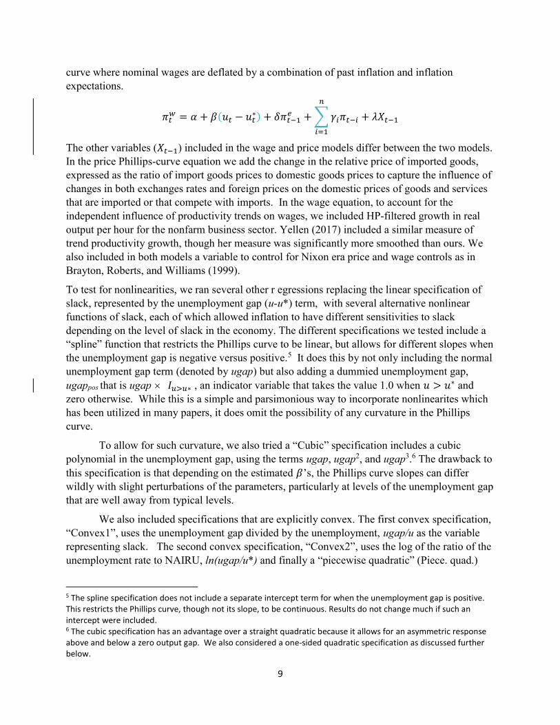
curve where nominal wages are deflated by a combination of past inflation and inflation expectations.

𝜋 = 𝛼 + 𝛽(𝑢 − 𝑢∗) + 𝛿𝜋 + 𝛾 𝜋 + 𝜆𝑋

The other variables (𝑋 ) included in the wage and price models differ between the two models. In the price Phillips-curve equation we add the change in the relative price of imported goods, expressed as the ratio of import goods prices to domestic goods prices to capture the influence of changes in both exchanges rates and foreign prices on the domestic prices of goods and services that are imported or that compete with imports. In the wage equation, to account for the independent influence of productivity trends on wages, we included HP-filtered growth in real output per hour for the nonfarm business sector. Yellen (2017) included a similar measure of trend productivity growth, though her measure was significantly more smoothed than ours. We also included in both models a variable to control for Nixon era price and wage controls as in Brayton, Roberts, and Williams (1999).

To test for nonlinearities, we ran several other r egressions replacing the linear specification of slack, represented by the unemployment gap (u-u*) term, with several alternative nonlinear functions of slack, each of which allowed inflation to have different sensitivities to slack depending on the level of slack in the economy. The different specifications we tested include a “spline” function that restricts the Phillips curve to be linear, but allows for different slopes when the unemployment gap is negative versus positive.5 It does this by not only including the normal unemployment gap term (denoted by ugap) but also adding a dummied unemployment gap, ugappos

that is ugap 𝐼 ∗ , an indicator variable that takes the value 1.0 when 𝑢 > 𝑢∗ and zero otherwise. While this is a simple and parsimonious way to incorporate nonlinearites which has been utilized in many papers, it does omit the possibility of any curvature in the Phillips curve.

To allow for such curvature, we also tried a “Cubic” specification includes a cubic polynomial in the unemployment gap, using the terms ugap, ugap2, and ugap3.6 The drawback to this specification is that depending on the estimated 𝛽’s, the Phillips curve slopes can differ wildly with slight perturbations of the parameters, particularly at levels of the unemployment gap that are well away from typical levels.

We also included specifications that are explicitly convex. The first convex specification, “Convex1”, uses the unemployment gap divided by the unemployment, ugap/u as the variable representing slack. The second convex specification, “Convex2”, uses the log of the ratio of the unemployment rate to NAIRU, ln(ugap/u*) and finally a “piecewise quadratic” (Piece. quad.)

5 The spline specification does not include a separate intercept term for when the unemployment gap is positive. This restricts the Phillips curve, though not its slope, to be continuous. Results do not change much if such an intercept were included. 6 The cubic specification has an advantage over a straight quadratic because it allows for an asymmetric response above and below a zero output gap. We also considered a one-sided quadratic specification as discussed further below.

10

specification that uses a linear slack term, plus the squared value of that slack term, the unemployment gap, only when the gap is negative. This allows for one-sided nonlinearity in tight labor markets only, following the approach used by Nalewaik (2016).7 The additional variable in this case is 2

negugap , that is ugap2 𝐼 ∗, the indicator variable that takes the value

1.0 when 𝑢 > 𝑢∗ and zero otherwise. Murphy (2018) compares results from a similar set of nonlinear specifications.

2.3 Data

2.3.1 Inflation

For the dependent variable in the price Phillips curve, we focus on core (ex food and energy) PCE inflation, expressed as quarterly changes in seasonally adjusted price levels at annual rates. Our results are robust to using core CPI instead. Core inflation is preferred over headline because the occasional high volatility of food and energy prices due to idiosyncratic factors in those markets can bias/affect estimation results for reasons not represented in the standard Phillips-curve model. However, these data begin in the late 1950s (1957 for the core CPI and 1959 core PCE). Given that we are also interested in the behavior of inflation in the 1950s, for which there were periods with an extraordinarily tight labor market, we also examine headline PCE inflation which goes back to the late 1940s.

For the wage Phillips curve, we look at several measures of wage inflation. One is the quarterly annualized (log) change in average hourly earnings for production and nonsupervisory workers, which begins in 1962 and covers about 80% of total private workers. For a more comprehensive measure that goes back further we also utilize compensation per hour for the nonfarm business sector; this series starts in 1947 but is more volatile than the other wage inflation measures. We also tested the employment cost index, including both the wages and salaries component and total compensation, which includes benefits. These series are more comprehensive than average hourly earnings and less volatile than compensation per hour, but they do not begin until 1982. Finally, we ran tests with unit labor cost inflation, or compensation per hour growth minus productivity growth in the nonfarm business sector (also back to the late 1940s); the productivity trend variable was dropped from the right hand side of these equations. In estimation, all price and wage inflation variables are expressed as (log) quarter to quarter changes in prices or wages at annual rates.

2.3.2 Slack

Our preferred measure of slack is the U-3 unemployment rate minus the Congressional Budget Office’s published estimate of the natural rate of unemployment or NAIRU. As is evident from Figure 2.1, the labor market tightened tremendously during the 1950s and 1960s,

7 This specification is does not allow the linear term to differ when the unemployment gap is above or below zero. This restriction forces the slope of the Phillips curve to be continuous and change smoothly as the unemployment rate passes through NAIRU unlike the spline specification where the slope is discretely different above and below NAIRU.

11

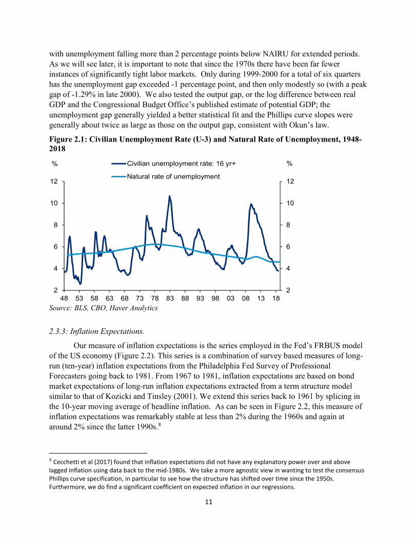
with unemployment falling more than 2 percentage points below NAIRU for extended periods. As we will see later, it is important to note that since the 1970s there have been far fewer instances of significantly tight labor markets. Only during 1999-2000 for a total of six quarters has the unemployment gap exceeded -1 percentage point, and then only modestly so (with a peak gap of -1.29% in late 2000). We also tested the output gap, or the log difference between real GDP and the Congressional Budget Office’s published estimate of potential GDP; the unemployment gap generally yielded a better statistical fit and the Phillips curve slopes were generally about twice as large as those on the output gap, consistent with Okun’s law.

Figure 2.1: Civilian Unemployment Rate (U-3) and Natural Rate of Unemployment, 1948-2018

Source: BLS, CBO, Haver Analytics

2.3.3: Inflation Expectations.

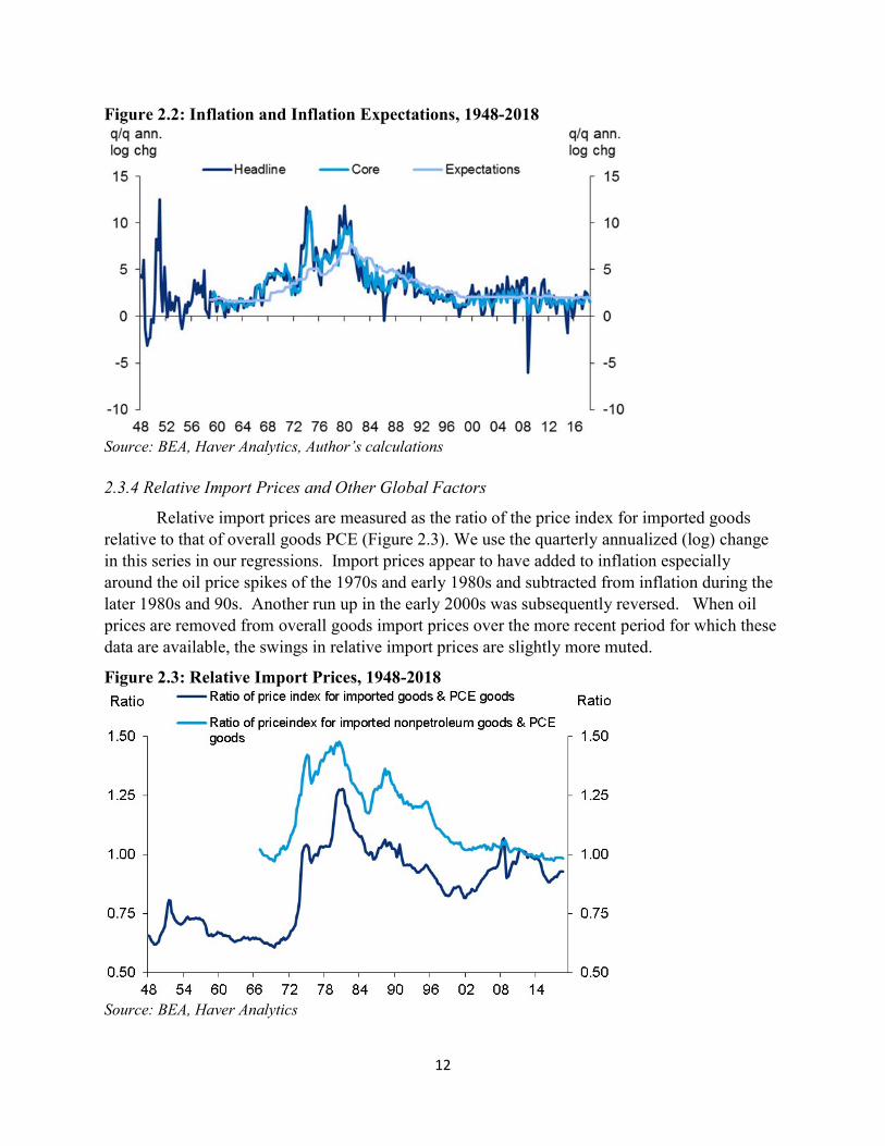
Our measure of inflation expectations is the series employed in the Fed’s FRBUS model of the US economy (Figure 2.2). This series is a combination of survey based measures of long-run (ten-year) inflation expectations from the Philadelphia Fed Survey of Professional Forecasters going back to 1981. From 1967 to 1981, inflation expectations are based on bond market expectations of long-run inflation expectations extracted from a term structure model similar to that of Kozicki and Tinsley (2001). We extend this series back to 1961 by splicing in the 10-year moving average of headline inflation. As can be seen in Figure 2.2, this measure of inflation expectations was remarkably stable at less than 2% during the 1960s and again at around 2% since the latter 1990s.8

8 Cecchetti et al (2017) found that inflation expectations did not have any explanatory power over and above lagged inflation using data back to the mid-1980s. We take a more agnostic view in wanting to test the consensus Phillips curve specification, in particular to see how the structure has shifted over time since the 1950s. Furthermore, we do find a significant coefficient on expected inflation in our regressions.

2

4

6

8

10

12

2

4

6

8

10

12

48 53 58 63 68 73 78 83 88 93 98 03 08 13 18

Civilian unemployment rate: 16 yr+

Natural rate of unemployment

% %

12

Figure 2.2: Inflation and Inflation Expectations, 1948-2018

Source: BEA, Haver Analytics, Author’s calculations 2.3.4 Relative Import Prices and Other Global Factors

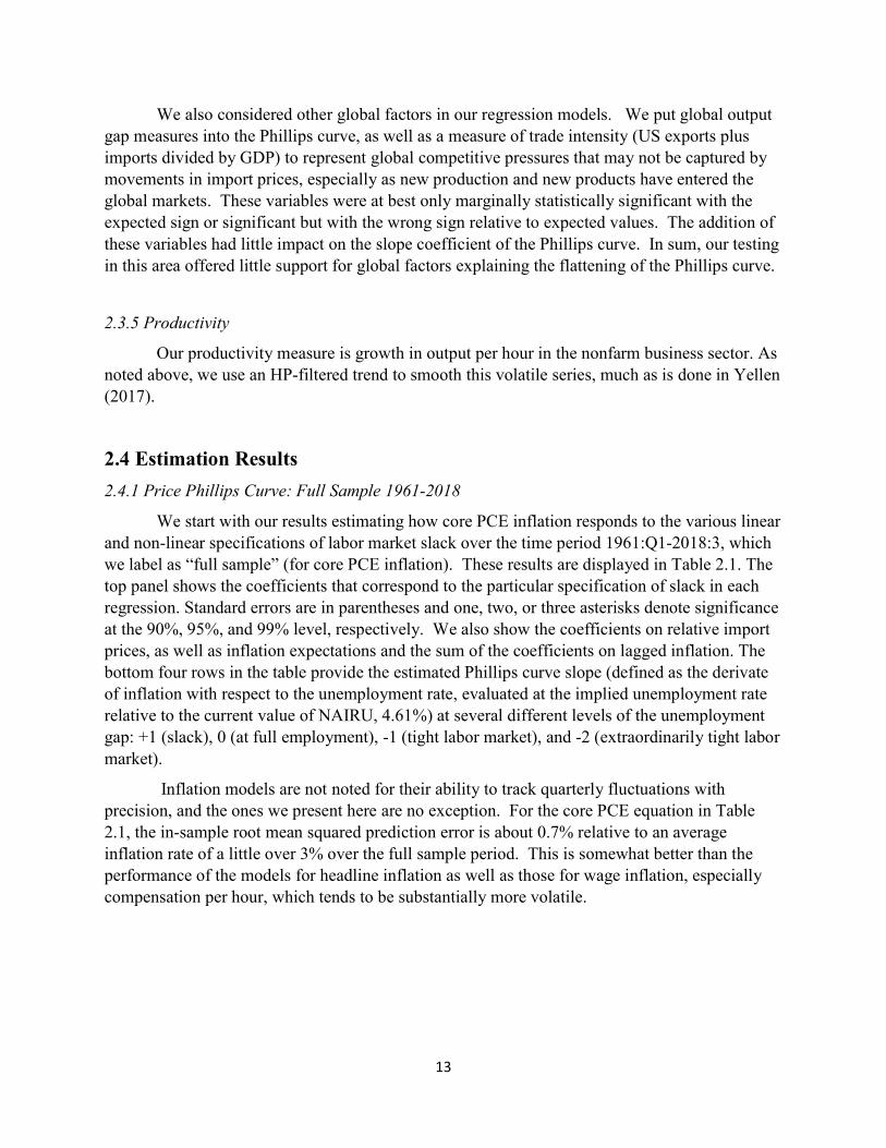
Relative import prices are measured as the ratio of the price index for imported goods relative to that of overall goods PCE (Figure 2.3). We use the quarterly annualized (log) change in this series in our regressions. Import prices appear to have added to inflation especially around the oil price spikes of the 1970s and early 1980s and subtracted from inflation during the later 1980s and 90s. Another run up in the early 2000s was subsequently reversed. When oil prices are removed from overall goods import prices over the more recent period for which these data are available, the swings in relative import prices are slightly more muted.

Figure 2.3: Relative Import Prices, 1948-2018

Source: BEA, Haver Analytics

13

We also considered other global factors in our regression models. We put global output gap measures into the Phillips curve, as well as a measure of trade intensity (US exports plus imports divided by GDP) to represent global competitive pressures that may not be captured by movements in import prices, especially as new production and new products have entered the global markets. These variables were at best only marginally statistically significant with the expected sign or significant but with the wrong sign relative to expected values. The addition of these variables had little impact on the slope coefficient of the Phillips curve. In sum, our testing in this area offered little support for global factors explaining the flattening of the Phillips curve.

2.3.5 Productivity

Our productivity measure is growth in output per hour in the nonfarm business sector. As noted above, we use an HP-filtered trend to smooth this volatile series, much as is done in Yellen (2017).

2.4 Estimation Results

2.4.1 Price Phillips Curve: Full Sample 1961-2018

We start with our results estimating how core PCE inflation responds to the various linear and non-linear specifications of labor market slack over the time period 1961:Q1-2018:3, which we label as “full sample” (for core PCE inflation). These results are displayed in Table 2.1. The top panel shows the coefficients that correspond to the particular specification of slack in each regression. Standard errors are in parentheses and one, two, or three asterisks denote significance at the 90%, 95%, and 99% level, respectively. We also show the coefficients on relative import prices, as well as inflation expectations and the sum of the coefficients on lagged inflation. The bottom four rows in the table provide the estimated Phillips curve slope (defined as the derivate of inflation with respect to the unemployment rate, evaluated at the implied unemployment rate relative to the current value of NAIRU, 4.61%) at several different levels of the unemployment gap: +1 (slack), 0 (at full employment), -1 (tight labor market), and -2 (extraordinarily tight labor market).

Inflation models are not noted for their ability to track quarterly fluctuations with precision, and the ones we present here are no exception. For the core PCE equation in Table 2.1, the in-sample root mean squared prediction error is about 0.7% relative to an average inflation rate of a little over 3% over the full sample period. This is somewhat better than the performance of the models for headline inflation as well as those for wage inflation, especially compensation per hour, which tends to be substantially more volatile.

14

Table 2.1: Core PCE Phillips Curve, Full Sample: 1961-2018

In the linear specification in Table 2.1, the full sample Phillips curve slope is relatively flat at -0.14, implying that a drop in the unemployment gap from 0 to -1% will raise inflation by 0.14% on impact--a pretty small effect overall. In the spline specification, the slope is considerably steeper at – 0.42 when the gap is below zero, but very close to zero at -0.05 when it is above zero (this is derived as the sum of the coefficients on the ugap and the ugappos term). This result suggests a substantial nonlinearity, which holds up to a considerable extent across the other nonlinear specifications (Cubic, Convex1, Convex 2 and Piece quad). The slope when the gap is at -1% (not too far from its recent level) ranges from -0.25 to -0.38. When the gap moves to +1, the slopes are noticeably smaller, ranging from -.08 to -.16.

If the labor market tightens to more extraordinary levels at two percentage points below NAIRU, the slope of the Phillips curve generally steepens even more. The persistence of inflation, gauged by the sum of the coefficients on lagged inflation is generally fairly high across

ugap -0.141 *** -0.423 *** -0.210 *** -0.082 **

ugappos 0.374 ***

ugap2

0.072 **

ugap3

-0.009

ugap/u -1.033 ***

ln(u/u*) -0.913 ***

ugapneg2 0.150 ***

Rel. Imp. Goods Infl. 0.035 *** 0.037 *** 0.037 *** 0.036 *** 0.036 *** 0.038 ***

Infl. Expectations 0.193 *** 0.231 *** 0.235 *** 0.218 *** 0.205 *** 0.239 ***

Sum Lag Infl. Coeffs.

RMSE

Slope at

ugap = +1 (u = 5.61)

ugap = 0 (u = 4.61)

ugap = -1 (u = 3.61)

ugap = -2 (u = 2.61)Standard errors in parentheses. ∗ p < 0.05, ∗∗ p < 0.01, ∗∗∗ p < 0.001

0.807 0.769 0.765 0.782 0.795

0.727 0.710 0.713 0.718 0.724

Linear Piece. quad.Convex2Convex1CubicSpline

Linear Spline Cubic Convex1

-0.141

-0.141

-0.141

-0.141 -0.423

-0.423

-0.048

-0.602

-0.380

-0.210

-0.092

-0.699

-0.365

-0.224

-0.151

Convex2 Piece. quad.

-0.350

-0.253

-0.198

-0.163

-0.682

-0.382

-0.082

-0.082

0.715

0.761

(0.049)

(0.207)

(0.058)

(0.009)

(0.060)

(0.009) (0.009)

(0.062)

(0.041)(0.057)(0.085)

(0.058)

(0.009) (0.009)

(0.058) (0.062)

(0.009)

(0.036)

(0.204)

(0.008)

(0.028)

(0.110)

15

all of the linear and nonlinear specifications. The coefficients on inflation expectations are relatively small but consistently highly statistically significant.

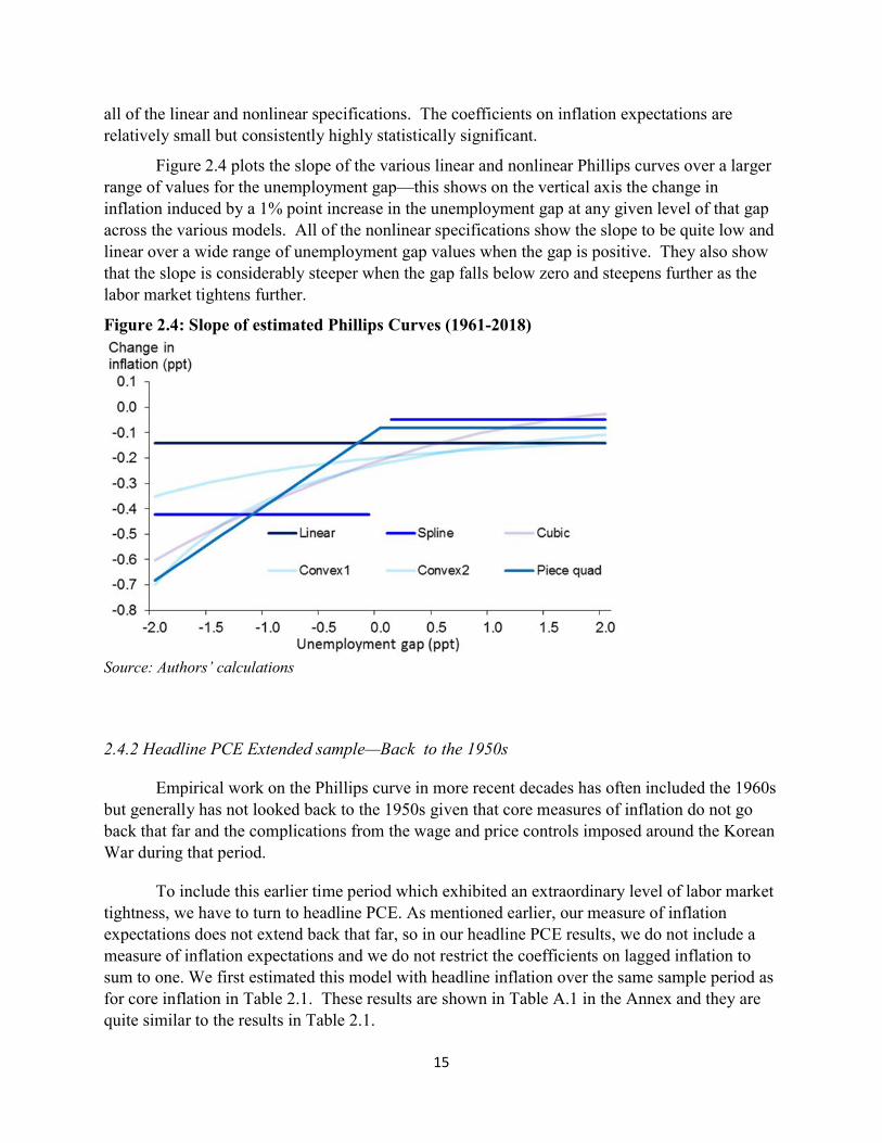
Figure 2.4 plots the slope of the various linear and nonlinear Phillips curves over a larger range of values for the unemployment gap—this shows on the vertical axis the change in inflation induced by a 1% point increase in the unemployment gap at any given level of that gap across the various models. All of the nonlinear specifications show the slope to be quite low and linear over a wide range of unemployment gap values when the gap is positive. They also show that the slope is considerably steeper when the gap falls below zero and steepens further as the labor market tightens further.

Figure 2.4: Slope of estimated Phillips Curves (1961-2018)


2.4.2 Headline PCE Extended sample—Back to the 1950s

Empirical work on the Phillips curve in more recent decades has often included the 1960s but generally has not looked back to the 1950s given that core measures of inflation do not go back that far and the complications from the wage and price controls imposed around the Korean War during that period.

To include this earlier time period which exhibited an extraordinary level of labor market tightness, we have to turn to headline PCE. As mentioned earlier, our measure of inflation expectations does not extend back that far, so in our headline PCE results, we do not include a measure of inflation expectations and we do not restrict the coefficients on lagged inflation to sum to one. We first estimated this model with headline inflation over the same sample period as for core inflation in Table 2.1. These results are shown in Table A.1 in the Annex and they are quite similar to the results in Table 2.1.

16

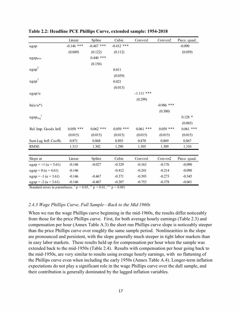
In Table 2.2, we show results for the sample period extended back to 1954. We see a slightly steeper slope of the Phillips curve in the linear case and the majority of the nonlinear cases, particularly around the levels of the unemployment gap seen in the latter 1950s. The persistence of inflation rises, but this may be in part because we were not able to include an inflation expectations variable in this case.9 In brief the addition of the experience during the tight labor market period of the mid-latter 1950s bolsters the results we found back to the early 1960s.

We also ran the equations over the full range of available data, back to 1949 (Annex Table A.2), attempting to account for the price and wage controls implemented around the Korean War much as Brayton, Roberts, and Williams (1999) did for the Nixon era controls. In this case, the slope was estimated to be much flatter than the post-1954 and post-1961 samples. The instability of the price Phillips curve equation over the early 1950s could well reflect a failure of our effort to account for the effects of the Korean War price controls, but it could also warrant further investigation.

9 With the absence of an inflation expectations tem, we also dropped the constraint on the lagged price coefficients (having them plus the expectations coefficient sum to 1.0). The Lagged price coefficients may be picking up more of the expectations effect in this case.

17

Table 2.2: Headline PCE Phillips Curve, extended sample: 1954-2018

2.4.3 Wage Phillips Curve, Full Sample—Back to the Mid 1960s

When we run the wage Phillips curve beginning in the mid-1960s, the results differ noticeably from those for the price Phillips curve. First, for both average hourly earnings (Table 2.3) and compensation per hour (Annex Table A.3) the short run Phillips curve slope is noticeably steeper than the price Phillips curve over roughly the same sample period. Nonlinearities in the slope are pronounced and persistent, with the slope generally much steeper in tight labor markets than in easy labor markets. These results held up for compensation per hour when the sample was extended back to the mid-1950s (Table 2.4). Results with compensation per hour going back to the mid-1950s, are very similar to results using average hourly earnings, with no flattening of the Phillips curve even when including the early 1950s (Annex Table A.4). Longer-term inflation expectations do not play a significant role in the wage Phillips curve over the dull sample, and their contribution is generally dominated by the lagged inflation variables.

ugap -0.146 *** -0.467 *** -0.412 *** -0.090

ugappos 0.440 ***

ugap2

0.011

ugap3

0.021

ugap/u -1.111 ***

ln(u/u*) -0.986 ***

ugapneg2 0.128 *



RMSE

Slope at

ugap = +1 (u = 5.61)

ugap = 0 (u = 4.61)

ugap = -1 (u = 3.61)


1.3101.313 1.302 1.290 1.305 1.309

(0.015)

0.871 0.868 0.893 0.870 0.869 0.867

(0.015) (0.015) (0.015) (0.015) (0.015)

(0.039)

(0.013)

(0.299)

(0.300)

(0.065)

(0.049) (0.122) (0.112) (0.059)

(0.156)

Piece. quad.Linear Spline Cubic Convex1 Convex2

-0.752

-0.393

-0.241

-0.163

-0.207

-0.371

-0.412

-0.146

-0.146

-0.146

-0.467

-0.467

-0.027

-0.601

-0.345

-0.090

-0.090

Linear Spline Cubic Convex1 Convex2

-0.329

-0.378

-0.273

-0.214

-0.176

Piece. quad.

-0.146

18

Table 2.3: Wage Phillips Curve (Average Hourly Earnings): 1964-2018

ugap -0.379 *** -0.611 *** -0.874 *** -0.365 ***

ugappos 0.294

ugap2

-0.092 *

ugap3

0.056 ***

ugap/u -2.519 ***

ln(u/u*) -2.344 ***

ugapneg2 0.041

Trend prod. growth. 0.471 *** 0.420 *** 0.272 ** 0.415 *** 0.440 *** 0.460 ***

Infl. Expectations 0.043 0.077 -0.006 0.097 0.071 0.056


RMSE

Slope at

ugap = +1 (u = 5.61)

ugap = 0 (u = 4.61)

ugap = -1 (u = 3.61)


Piece. quad.

Linear Spline Cubic Convex1 Convex2 Piece. quad.


-0.898

-0.649

-0.509

-0.418

(0.050)

(0.014)

(0.461)

(0.474)

Convex2

-0.530

-0.448

-0.365

-0.365

0.171

-0.521

-0.874

-0.889

-1.705

-0.891

-0.546

-0.369

-0.379

-0.379

-0.379

-0.379

-0.611

-0.611

-0.317

(0.081) (0.176) (0.125) (0.089)

(0.214)

(0.086)

(0.103) (0.109) (0.107) (0.106) (0.106) (0.106)

(0.122)

0.957 0.923 1.006 0.903 0.929 0.944

(0.109) (0.117) (0.113) (0.114) (0.112)

1.2981.295 1.293 1.218 1.294 1.299

19

Table 2.4: Wage Phillips Curve (Compensation per Hour): 1954-2018

Note: Inflation expectations are not included. The seven lags of core PCE inflation are constrained to sum to 1.0.

2.4.4 Stability over Time: More Recent Sample 1988-2018

Ample recent empirical literature and the rolling regression results we included in the introduction to this paper say that the slope of the Phillips curve has flattened significantly over time. But they do not have much to say about the potential steepening of the Phillips curve due to nonlinearities, if the labor market continues to tighten. That is the subject of our next set of tests: even if the overall slope has flattened, could it still bounce back if the unemployment gap falls persistently below -1%?

Price-Phillips curve has flattened.

Table 2.5 and Figure 2.5 presents results parallel to those in Table 2.1 and Figure 2.4, for the price Phillips curve, but with estimation starting in 1988. This starting point was selected as being both near the midpoint of our core full sample, and at a point where our rolling regression

ugap -0.403 *** -0.927 *** -0.646 ** -0.297 *

ugappos 0.714 **

ugap2

0.062

ugap3

0.008

ugap/u -2.747 ***

ln(u/u*) -2.587 ***

ugapneg2 -0.239 *

Trend prod. growth. 0.631 *** 0.608 ** 0.569 ** 0.601 ** 0.605 ** 0.627 ***

RMSE

Slope at

ugap = +1 (u = 5.61)

ugap = 0 (u = 4.61)

ugap = -1 (u = 3.61)


Piece. quad.



-0.991

-0.717

-0.561

-0.461

(0.091)

(0.030)

(0.761)

(0.837)

Convex2

0.661

0.182

-0.297

-0.297

-0.802

-0.748

-0.646

-0.498

-1.859

-0.972

-0.596

-0.402

-0.403

-0.403

-0.403

-0.403

-0.927

-0.927

-0.213

(0.144) (0.238) (0.254) (0.178)

(0.342)

(0.137)

(0.238) (0.237) (0.235) (0.235) (0.235) (0.237)

2.7062.710 2.698 2.706 2.699 2.705

20

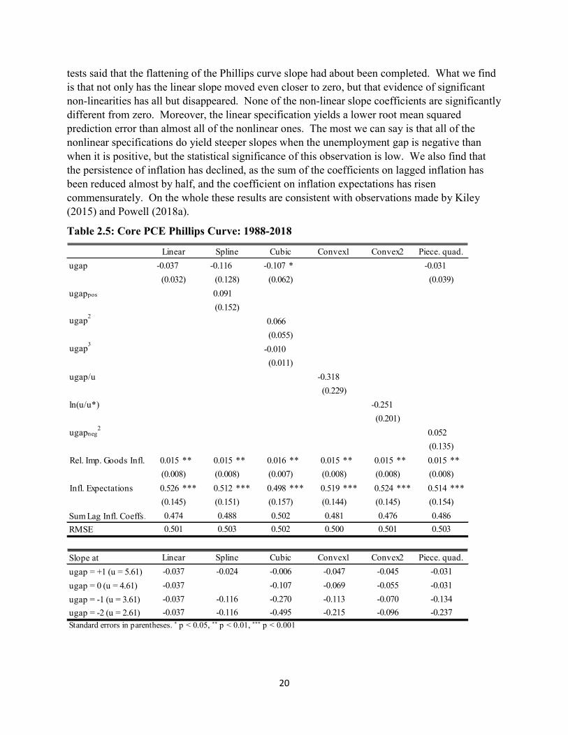
tests said that the flattening of the Phillips curve slope had about been completed. What we find is that not only has the linear slope moved even closer to zero, but that evidence of significant non-linearities has all but disappeared. None of the non-linear slope coefficients are significantly different from zero. Moreover, the linear specification yields a lower root mean squared prediction error than almost all of the nonlinear ones. The most we can say is that all of the nonlinear specifications do yield steeper slopes when the unemployment gap is negative than when it is positive, but the statistical significance of this observation is low. We also find that the persistence of inflation has declined, as the sum of the coefficients on lagged inflation has been reduced almost by half, and the coefficient on inflation expectations has risen commensurately. On the whole these results are consistent with observations made by Kiley (2015) and Powell (2018a).

Table 2.5: Core PCE Phillips Curve: 1988-2018

ugap -0.037 -0.116 -0.107 * -0.031

ugappos 0.091

ugap2

0.066

ugap3

-0.010

ugap/u -0.318

ln(u/u*) -0.251

ugapneg2

0.052

Rel. Imp. Goods Infl. 0.015 ** 0.015 ** 0.016 ** 0.015 ** 0.015 ** 0.015 **

Infl. Expectations 0.526 *** 0.512 *** 0.498 *** 0.519 *** 0.524 *** 0.514 ***


RMSE

Slope at

ugap = +1 (u = 5.61)

ugap = 0 (u = 4.61)

ugap = -1 (u = 3.61)



Linear Piece. quad.Convex2Convex1CubicSpline


-0.037

-0.037

-0.037

0.474 0.488 0.502 0.481

(0.055)

(0.011)

(0.229)

(0.145)

-0.037 -0.116

-0.116

-0.024

-0.495

-0.270

-0.107

-0.006

-0.215

-0.113

-0.069

-0.047

-0.096

-0.070

-0.055

-0.045

-0.237

-0.134

-0.031

-0.031

0.476 0.486

0.501 0.503 0.502 0.500 0.501 0.503

(0.039)(0.062)(0.128)(0.032)

(0.152)

(0.201)

(0.135)

(0.008) (0.008) (0.007) (0.008) (0.008) (0.008)

(0.154)(0.145)(0.144)(0.157)(0.151)

21

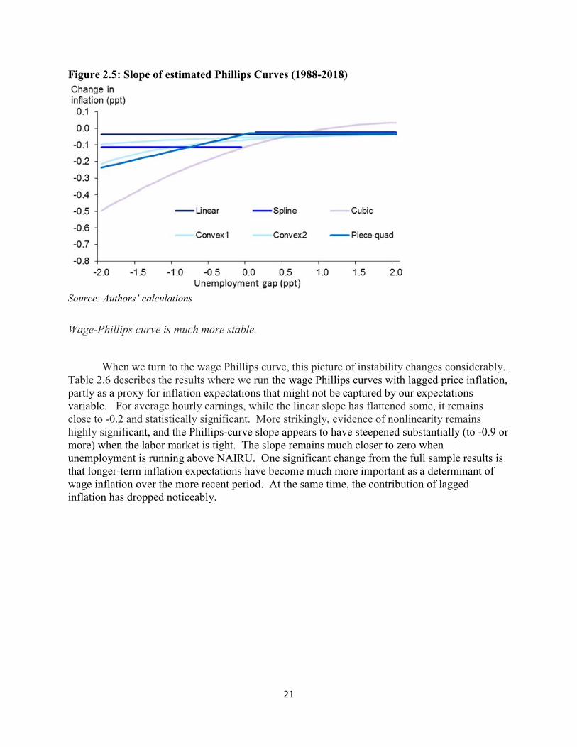
Figure 2.5: Slope of estimated Phillips Curves (1988-2018)


Wage-Phillips curve is much more stable.

When we turn to the wage Phillips curve, this picture of instability changes considerably.. Table 2.6 describes the results where we run the wage Phillips curves with lagged price inflation, partly as a proxy for inflation expectations that might not be captured by our expectations variable. For average hourly earnings, while the linear slope has flattened some, it remains close to -0.2 and statistically significant. More strikingly, evidence of nonlinearity remains highly significant, and the Phillips-curve slope appears to have steepened substantially (to -0.9 or more) when the labor market is tight. The slope remains much closer to zero when unemployment is running above NAIRU. One significant change from the full sample results is that longer-term inflation expectations have become much more important as a determinant of wage inflation over the more recent period. At the same time, the contribution of lagged inflation has dropped noticeably.

22

Table 2.6: Wage Phillips Curve (Average Hourly Earnings): 1988-2018

Broadly similar results are found across the other measures of wage inflation that we tested, as seen in Table 2.7. Here we report a subset of the models, including the linear version and the spline specification to represent the nonlinear, across the different wage measures, including compensation per hour, ECI total compensation, ECI wages and salaries, and unit labor costs. In general, these results show short run Phillips curve slopes in the vicinity of -0.2 to -0.3, considerably steeper than for the price Phillips curves over this period. They also show substantial nonlinearities, with the slope much steeper in tight labor markets than easy labor markets. Productivity growth is a significant contributor throughout. Inflation expectations have become much more important and lagged inflation much less important than over the full sample period.

ugap -0.180 *** -0.929 *** -0.656 *** -0.123 **

ugappos 0.840 ***

ugap2

0.123 *

ugap3

0.003

ugap/u -1.809 ***

ln(u/u*) -1.318 ***

ugapneg2 0.694 ***

Trend prod. growth 0.439 *** 0.328 *** 0.280 *** 0.358 *** 0.403 *** 0.320 ***

Infl. Expectations 0.627 * 0.546 0.430 0.639 * 0.639 * 0.515


RMSE

Slope at

ugap = +1 (u = 5.61)

ugap = 0 (u = 4.61)

ugap = -1 (u = 3.61)


(0.383)(0.380) (0.372) (0.365) (0.366) (0.375)

(0.245)

(0.097) (0.098) (0.100) (0.097) (0.097) (0.097)

(0.279)

(0.073)

(0.014)

(0.404)

(0.349)

0.485

0.895 0.872 0.838 0.872 0.886 0.877

0.373 0.454 0.570 0.361 0.361

(0.055) (0.248) (0.123) (0.060)

-0.180

-0.180

-0.180

-0.180

-0.929

-0.929

-0.089

-2.898

-1.511

-0.123

-0.123

-1.111

-0.893

-0.656

-0.400

-1.224

-0.640

-0.392

-0.265

Cubic Convex1

-0.505

-0.365

-0.286

-0.235



Linear Spline

23

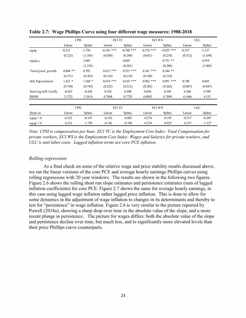
Table 2.7: Wage Phillips Curve using four different wage measures: 1988-2018

Note: CPH is compensation per hour, ECI TC is the Employment Cost Index: Total Compensation for private workers, ECI WS is the Employment Cost Index: Wages and Salaries for private workers, and ULC is unit labor costs. Lagged inflation terms are core PCE inflation.

Rolling regressions

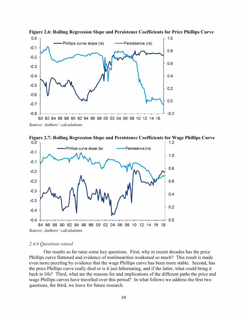
As a final check on some of the relative wage and price stability results discussed above, we ran the linear versions of the core PCE and average hourly earnings Phillips curves using rolling regressions with 20 year windows. The results are shown in the following two figures. Figure 2.6 shows the rolling short run slope estimates and persistence estimates (sum of lagged inflation coefficients) for core PCE. Figure 2.7 shows the same for average hourly earnings, in this case using lagged wage inflation rather lagged price inflation. This is done to allow for some dynamics in the adjustment of wage inflation to changes in its determinants and thereby to test for “persistence” in wage inflation. Figure 2.6 is very similar to the picture reported by Powell (2018a), showing a sharp drop over time in the absolute value of the slope, and a more recent plunge in persistence. The picture for wages differs: both the absolute value of the slope and persistence decline over time, but much less, and to significantly more elevated levels than their price Phillips curve counterparts.

ugap -0.321 -1.750 -0.156 *** -0.748 *** -0.274 *** -0.925 *** -0.337 -1.127

ugappos 1.603 0.665 0.731 ** 0.919

Trend prod. growth 0.804 ** 0.592 0.612 *** 0.523 *** 0.341 *** 0.244 **

Infl. Expectations 1.423 * 1.268 * 0.674 *** 0.610 *** 0.962 *** 0.891 *** 0.740 0.602


RMSE

Slope at

ugap > 0

ugap < 0

0.398

(1.650)

(1.805)

(0.887) (0.847)(0.282) (0.262)

0.038 0.109

(0.312)

0.260

(0.050) (0.051) (0.278)

(0.288)

(0.109) (0.119)

0.390

(0.212)

(0.129)

(0.301)

(0.289)

(0.742)(0.744)

-0.268-0.423

(0.116)

(0.222)

0.326

(0.223) (1.105)

(1.218)

(0.383)(0.371)

CPH ECI TC ECI WS ULC

SplineLinearSplineLinearSplineLinearSplineLinear

4.1446 4.155

Linear Spline Linear

3.3725 3.3614 0.7888 0.8092 0.7899

-0.321 -0.147 -0.156 -0.083

0.7729

-0.207

-0.337 -1.127


Linear Spline Linear Spline

-0.321 -1.750 -0.156 -0.748

Spline

-0.274 -0.195

-0.274 -0.925

-0.337

24

Figure 2.6: Rolling Regression Slope and Persistence Coefficients for Price Phillips Curve


Figure 2.7: Rolling Regression Slope and Persistence Coefficients for Wage Phillips Curve


2.4.6 Questions raised

Our results so far raise some key questions. First, why in recent decades has the price Phillips curve flattened and evidence of nonlinearities weakened so much? This result is made even more puzzling by evidence that the wage Phillips curve has been more stable. Second, has the price Phillips curve really died or is it just hibernating, and if the latter, what could bring it back to life? Third, what are the reasons for and implications of the different paths the price and wage Phillips curves have travelled over this period? In what follows we address the first two questions, the third, we leave for future research.

25

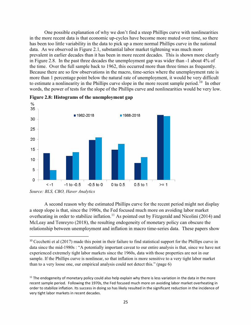
One possible explanation of why we don’t find a steep Phillips curve with nonlinearities in the more recent data is that economic up-cycles have become more muted over time, so there has been too little variability in the data to pick up a more normal Phillips curve in the national data. As we observed in Figure 2.1, substantial labor market tightening was much more prevalent in earlier decades than it has been in more recent decades. This is shown more clearly in Figure 2.8. In the past three decades the unemployment gap was wider than -1 about 4% of the time. Over the full sample back to 1962, this occurred more than three times as frequently. Because there are so few observations in the macro, time-series where the unemployment rate is more than 1 percentage point below the natural rate of unemployment, it would be very difficult to estimate a nonlinearity in the Phillips curve slope in the more recent sample period.10 In other words, the power of tests for the slope of the Phillips curve and nonlinearities would be very low.

Figure 2.8: Histograms of the unemployment gap


A second reason why the estimated Phillips curve for the recent period might not display a steep slope is that, since the 1980s, the Fed focused much more on avoiding labor market overheating in order to stabilize inflation.11 As pointed out by Fitzgerald and Nicolini (2014) and McLeay and Tenreyro (2018), the resulting endogeneity of monetary policy can obscure the relationship between unemployment and inflation in macro time-series data. These papers show

10 Cecchetti et al (2017) made this point in their failure to find statistical support for the Phillips curve in data since the mid-1980s : “A potentially important caveat to our entire analysis is that, since we have not experienced extremely tight labor markets since the 1960s, data with those properties are not in our sample. If the Phillips curve is nonlinear, so that inflation is more sensitive to a very tight labor market than to a very loose one, our empirical analysis could not detect this.” (page 6)

11 The endogeneity of monetary policy could also help explain why there is less variation in the data in the more recent sample period. Following the 1970s, the Fed focused much more on avoiding labor market overheating in order to stabilize inflation. Its success in doing so has likely resulted in the significant reduction in the incidence of very tight labor markets in recent decades.

26

that when monetary policy pursues a goal of minimizing welfare losses, measured as a sum of deviations of inflation from its target and deviations of output from potential (which is inversely related to the unemployment gap), monetary policy seeks to decrease inflation when the unemployment gap is negative. Endogenous monetary policy then induces a positive correlation between inflation and the unemployment gap that biases the slope coefficient of the Phillips curve toward zero. Indeed, in the Fitzgerald and Nicolini (2014) and McLeay and Tenroyo (2018) models, optimal monetary policy completely eliminates any correlation between inflation and the output gap (or equivalently the unemployment gap). This reasoning suggests that the Phillips curve slope in the regression estimates for the recent period likely understates the true steepness of the Phillips curve.

The models by Fitzgerald and Nicolini (2014) and McLeay and Tenroyo (2018) imply that empirical estimates of a flattening Phillips reflect a monetary policy that is more responsive to deviations in the unemployment gap. As a result, it would be a mistake to conclude that the flattening of the Phillips curve in the data implies that inflation would remain subdued with a significantly negative unemployment gap if the Fed responded more passively. The flattening reflects a responsive monetary policy, but we should expect a steepening if monetary policy were too accommodative.”

The argument above suggests that we might seek out data that not only has more variation than the macro, time-series data, but is also not subject to the possible bias created by endogenous monetary policy. A natural place to look is data for U.S. states and Metropolitan Statistical Areas (MSAs), because there are many more observations of very tight labor markets. Furthermore, monetary policy can be treated as exogenous in state and MSA data because monetary policy is national and so is the same for all states and MSAs. In Section 3, we provide evidence on the slope and nonlinearity in this data.

The third explanation for the flattening of the Phillips curve, and the one that has attracted by far the most attention in the literature, is the anchoring of inflation expectations. As we saw in Figure 2.2, for at least the past two decades, longer-term inflation expectations as gauged by the Survey of Professional Forecasters has been remarkably stable in the vicinity of 2%. This anchoring may have been bolstered by the Fed’s adoption of a specific 2% inflation objective in 2012, which was preceded by a decade during which that objective was widely seen as implicit, and a longer period during which the Fed had striven, successfully, to reduce inflation to that neighborhood from much higher levels. Inflation may have appeared reasonably well anchored during the 1960s, following a period (since the Korean War) during which it had averaged 2% or less. But that episode ended badly, in a great inflation. This leads to the question of could history repeat itself, or what might cause the Phillips curve to come out of hibernation again? We address this issue in Section 4, by taking a closer look at the experience of the 1960s and what led to the great inflation.

27

Section 3: Evidence from State and City Level Data

3.1 State and City Level Estimates

This section explores regional data in the United States to provide more insight into the relationship between the unemployment rate and inflation. One of the main advantages of regional data sets is that the typically contain a wider distribution of employment conditions than national level data.

Figure 3.1 shows the distribution of the unemployment rate for the United States as a whole (left panel) and for states within the United States (right panel) from 1980 to 2017. As the left panel shows, there is little precedent for the country as a whole for an unemployment rate below 4%. In contrast, as the right panel shows, there are several states that have experienced an unemployment rate below 4% during the 1980 to 2017 period. In fact, just over 15% of the observations of the state-year level panel have an unemployment rate below 4%. The mass of the distribution in the state-year level data below 4% can help identify the slope of the Phillips curve during low unemployment rate situations such as the United States is experiencing currently.

Figure 3.1: Distribution of the Unemployment Rate, 1980-2017

A. Aggregate

Source: BLS

28

B. States

Source: BLS

The data used in this section are detailed in two studies: Kumar and Orrenius (2016) for the wage-Phillips curve estimation at the state level from 1981 to 2017, and Babb and Detmeister (2017) for the price-Phillips curve estimation at the MSA-level from 1990 to 2017. For the wage-Phillips estimation at the state level, the state unemployment rates are calculated from the monthly Current Population Survey. The state-level wages are average hourly wage rates calculated from the monthly CEPR uniform extracts of CPS outgoing rotation groups. State-level price inflation rates are not available for this full time frame. As a result, the core inflation measure for the state-level analysis is based on price inflation from the CPI-U data by Census region. For the MSA level analysis, the unemployment rates at the city-year level come from the BLS, and the price inflation data are derived from the consumer price index for All Urban Consumers, and the specific measure is all items less food and energy.

Studies that rely on regional data to estimate the Phillips curve typically conduct regression specifications with both year and geography fixed effects. Given that inclusion of year fixed effects removes the aggregate time series variation that identifies national-level Phillips curve estimation, such an inclusion ensures that the identifying variation in state-level or MSA-level analysis is distinct from the identifying variation in national-level analysis. Put simply, the estimations seek to use a new source of variation to identify Phillips curve slope.

The inclusion of geography level-fixed effects helps ensure that cross-sectional differences in unobservable average differences across areas are not used to identify the Phillips curve relationship. For example, the natural unemployment rate may differ across states, and inclusion of state-fixed effects ensures that such a difference is not the identifying variation in a state-level Phillips curve estimation. Instead, the curve is identified using deviations in the unemployment rate from the average unemployment rate in a geographic area.

29

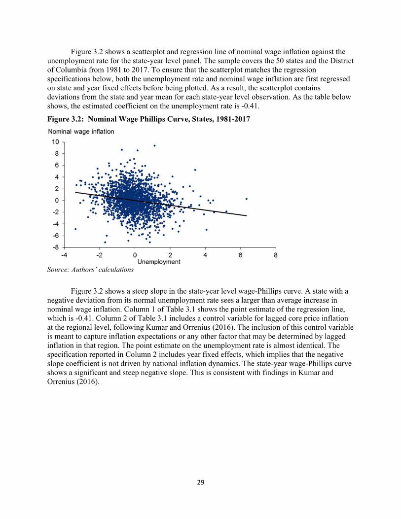
Figure 3.2 shows a scatterplot and regression line of nominal wage inflation against the unemployment rate for the state-year level panel. The sample covers the 50 states and the District of Columbia from 1981 to 2017. To ensure that the scatterplot matches the regression specifications below, both the unemployment rate and nominal wage inflation are first regressed on state and year fixed effects before being plotted. As a result, the scatterplot contains deviations from the state and year mean for each state-year level observation. As the table below shows, the estimated coefficient on the unemployment rate is -0.41.

Figure 3.2: Nominal Wage Phillips Curve, States, 1981-2017


Figure 3.2 shows a steep slope in the state-year level wage-Phillips curve. A state with a negative deviation from its normal unemployment rate sees a larger than average increase in nominal wage inflation. Column 1 of Table 3.1 shows the point estimate of the regression line, which is -0.41. Column 2 of Table 3.1 includes a control variable for lagged core price inflation at the regional level, following Kumar and Orrenius (2016). The inclusion of this control variable is meant to capture inflation expectations or any other factor that may be determined by lagged inflation in that region. The point estimate on the unemployment rate is almost identical. The specification reported in Column 2 includes year fixed effects, which implies that the negative slope coefficient is not driven by national inflation dynamics. The state-year wage-Phillips curve shows a significant and steep negative slope. This is consistent with findings in Kumar and Orrenius (2016).

30

Table 3.1: Wage Phillips Curve, State Level, 1981-2017

Log change in nominal wage

(1) (2) (3) (4) Unemployment rate, annual -0.410∗∗∗ -0.407∗∗∗ -1.000∗∗∗ -0.987∗∗

(0.049) (0.049) (0.300) (0.300)

Unemployment*(4 < Unemp ≤ 5.5)

0.389 0.388 (0.356) (0.356)

Unemployment*(5.5 < Unemp ≤ 7.5)

0.291 0.278 (0.339) (0.340)

Unemployment*(7.5 < Unemp) 0.807∗∗ 0.793∗ (0.307) (0.308)

Core inflation, lagged 0.180 0.131 (0.138) (0.138)

(4 < Unemp ≤ 5.5)

-1.698 -1.703 (1.422) (1.422)

(5.5 < Unemp ≤ 7.5)

-0.898 -0.830 (1.503) (1.505)

(7.5 < Unemp) -4.778∗∗∗ -4.698∗∗∗ (1.293) (1.296)

Level State State State State Source CEPR CEPR CEPR CEPR State effects Y Y Y Y

Year effects Y Y Y Y

N 1887 1887 1887 1887 R-sq 0.336 0.337 0.346 0.347

Standard errors in parentheses ∗ p < 0.05, ∗∗ p < 0.01, ∗∗∗ p < 0.001

The specifications in columns 3 and 4 test for non-linearity in the wage-Phillips curve. More specifically, the specification utilizes bins of state-year level data based on the unemployment rate. Unlike the national specification, the state-level specification cannot focus on the natural rate of unemployment because no such estimates are available at the state level. Instead, we follow Leduc, Marti, and Wilson (2019) and form the bins for the unemployment rate below 4%, between 4 and 5.5%, between 5.5 and 7.5%, and above 7.5%. For each bin, the specification includes both an indicator variable for each bin, and the bin variable interacted with the unemployment rate. The coefficient estimates on the interaction terms answer the following question: does the slope of the wage-Phillips curve change significantly when the level of the unemployment rate differs?

Columns 3 and 4 report the estimates, which are very similar. We focus on column 4, which are our preferred estimates because it makes sense to have lagged core inflation in the specification to reflect inflation expectations or any other factor that may be determined by lagged inflation in that region. The omitted group is the bin with an unemployment rate below

31

4%. For this group, the wage-Phillips curve is especially steep: -0.99. The interaction term coefficient estimates for the next two bins suggest a flatter wage-Phillips curve, but the point estimates are not statistically distinct from zero at a reasonable confidence level. However, the interaction term coefficient estimate for the bin of unemployment above 7.5% is 0.79 and statistically distinct from zero at the 5% confidence level. We should note that the results presented in Table 3.1 are qualitatively similar if the regression specifications are weighted by the labor force for each state-year observation.

Figure 3.3 plots the slope coefficient for each unemployment bin implied by the coefficient estimates in column 4 of Table 3.1. For the bin of observations with the unemployment rate below 4%, this is simply the point estimate from the top row of column 4. For the other bins, it is the point estimate from the top row of column 4 plus the estimated coefficient on the interaction term for the bin in question. Figure 4.3 shows that the wage-Phillips curve shows evidence of non-linearity, particularly when the unemployment rate exceeds 7.5%.

Figure 3.3: State-level Wage-Phillips Curve Coefficients by Unemployment Rate


The findings of Figure 3.3 are consistent with the analysis in Leduc et al (2019) of non-linearity in the state-year level wage-Phillips curve at higher levels of unemployment. The difference in the slope coefficient is statistically significant when the unemployment rate increases from below 7.5% to above 7.5%. The point estimate implies a flatter slope when the unemployment rate goes from below 4% to above 4%, but the difference is not statistically significant at a reasonable confidence level.

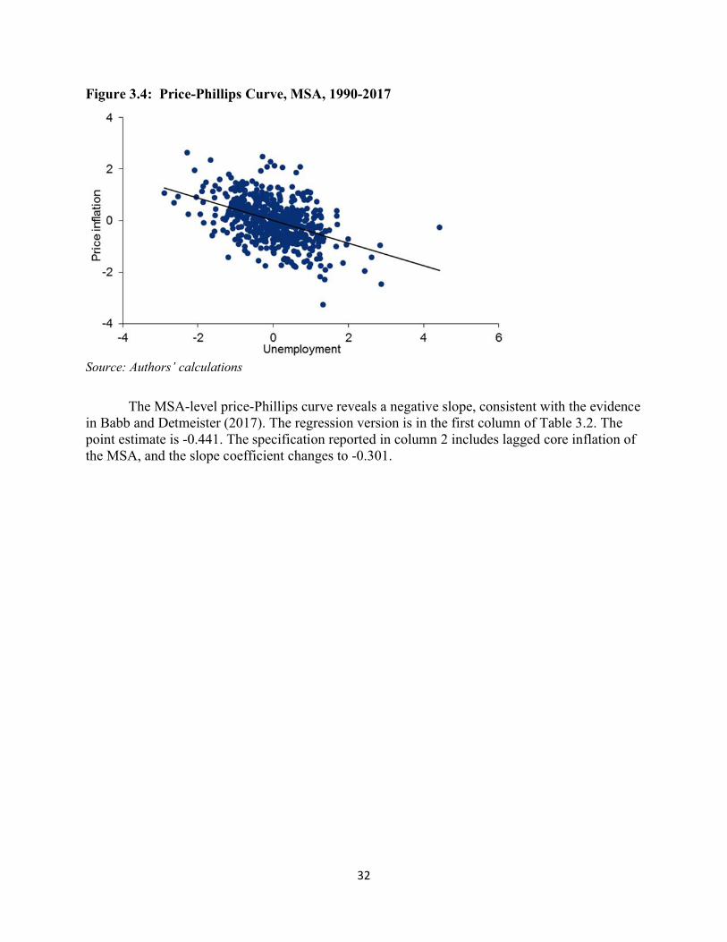
We next examine price-Phillips curve estimation. For consumer prices, the analysis follows Babb and Detmeister's (2017) analysis of 23 MSAs from 1990 to 2017. Figure 3.4 shows the price-Phillips scatterplot at the MSA level, where once again the MSA fixed effects and year fixed effects are removed.

32

Figure 3.4: Price-Phillips Curve, MSA, 1990-2017


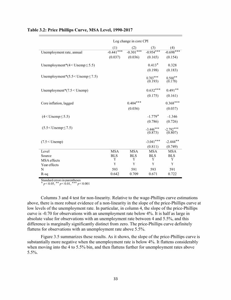
The MSA-level price-Phillips curve reveals a negative slope, consistent with the evidence in Babb and Detmeister (2017). The regression version is in the first column of Table 3.2. The point estimate is -0.441. The specification reported in column 2 includes lagged core inflation of the MSA, and the slope coefficient changes to -0.301.

33

Table 3.2: Price Phillips Curve, MSA Level, 1990-2017

Log change in core CPI

(1) (2) (3) (4) Unemployment rate, annual -0.441∗∗∗ -0.301∗∗∗ -0.954∗∗∗ -0.698∗∗∗

(0.037) (0.036) (0.165) (0.154)

Unemployment*(4 < Unemp ≤ 5.5)

0.413∗ 0.328 (0.198) (0.183)

Unemployment*(5.5 < Unemp ≤ 7.5) 0.703∗∗∗ (0.193)

0.560∗∗ (0.178)

Unemployment*(7.5 < Unemp) 0.632∗∗∗ 0.491∗∗ (0.175) (0.161)

Core inflation, lagged 0.404∗∗∗ 0.368∗∗∗ (0.036) (0.037)

(4 < Unemp ≤ 5.5)

-1.779∗ -1.346 (0.786) (0.726)

(5.5 < Unemp ≤ 7.5) -3.446∗∗∗ (0.873)

-2.792∗∗∗ (0.807)

(7.5 < Unemp) -3.041∗∗∗ -2.444∗∗ (0.811) (0.749)

Level MSA MSA MSA MSA Source BLS BLS BLS BLS MSA effects Y Y Y Y

Year effects Y Y Y Y

N 593 591 593 591 R-sq 0.642 0.709 0.671 0.722

Standard errors in parentheses ∗ p < 0.05, ∗∗ p < 0.01, ∗∗∗ p < 0.001

Columns 3 and 4 test for non-linearity. Relative to the wage-Phillips curve estimations above, there is more robust evidence of a non-linearity in the slope of the price-Phillips curve at low levels of the unemployment rate. In particular, in column 4, the slope of the price-Phillips curve is -0.70 for observations with an unemployment rate below 4%. It is half as large in absolute value for observations with an unemployment rate between 4 and 5.5%, and this difference is marginally significantly distinct from zero. The price-Phillips curve definitely flattens for observations with an unemployment rate above 5.5%.

Figure 3.5 summarizes these results. As it shows, the slope of the price-Phillips curve is substantially more negative when the unemployment rate is below 4%. It flattens considerably when moving into the 4 to 5.5% bin, and then flattens further for unemployment rates above 5.5%.

34

Figure 3.5: MSA-level Price-Phillips Curve Coefficients by Unemployment Rate


3.2 Comparing National and Regional Level Estimates

From a statistical perspective, it is important to emphasize that the national level and regional level estimates of the Phillips curve are exploiting different sources of variation. The regional level estimates are produced with specifications that include year fixed effects, and so the national level effect of unemployment on inflation is eliminated. As a result, from a purely statistical perspective, there is no reason to expect similarity between the national and regional level Phillips curve coefficients presented above.

That being said, the coefficient estimates for the wage-Phillips curve are similar for the national- and state-level specifications, both in terms of the level and the evidence for non-linearities. For example, in the national level data from 1988 to 2018 in Table 3.3, the slope of the wage-Phillips curve is between -0.29 and -0.35 depending on the measure of wage inflation used. In the state-level data, the slope is -0.41 for the sample from 1981 to 2017, and the estimate is similar if we restrict the sample to 1988 to 2017.

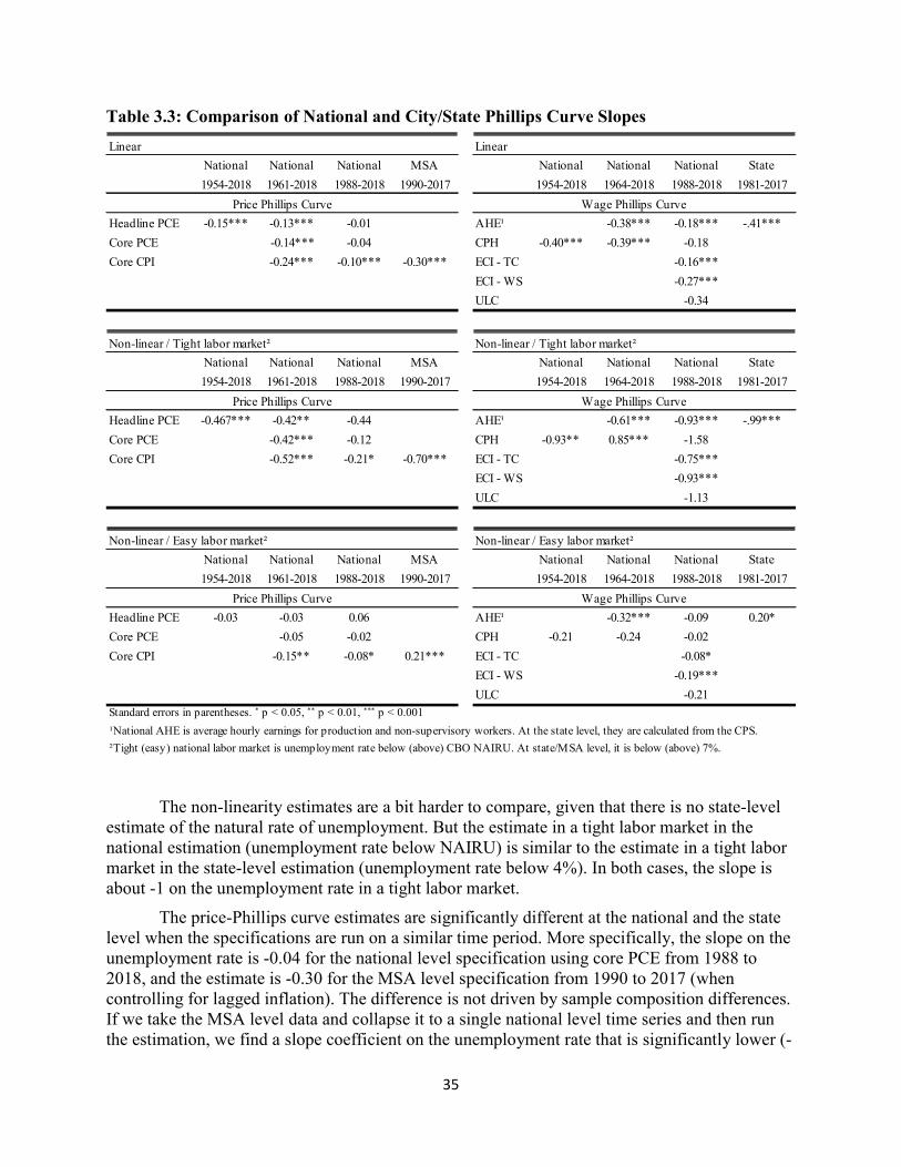
35

Table 3.3: Comparison of National and City/State Phillips Curve Slopes

The non-linearity estimates are a bit harder to compare, given that there is no state-level estimate of the natural rate of unemployment. But the estimate in a tight labor market in the national estimation (unemployment rate below NAIRU) is similar to the estimate in a tight labor market in the state-level estimation (unemployment rate below 4%). In both cases, the slope is about -1 on the unemployment rate in a tight labor market.

The price-Phillips curve estimates are significantly different at the national and the state level when the specifications are run on a similar time period. More specifically, the slope on the unemployment rate is -0.04 for the national level specification using core PCE from 1988 to 2018, and the estimate is -0.30 for the MSA level specification from 1990 to 2017 (when controlling for lagged inflation). The difference is not driven by sample composition differences. If we take the MSA level data and collapse it to a single national level time series and then run the estimation, we find a slope coefficient on the unemployment rate that is significantly lower (-

National National National MSA National National National State

1954-2018 1961-2018 1988-2018 1990-2017 1954-2018 1964-2018 1988-2018 1981-2017

Headline PCE -0.15*** -0.13*** -0.01 AHE¹ -0.38*** -0.18*** -.41***

Core PCE -0.14*** -0.04 CPH -0.40*** -0.39*** -0.18

Core CPI -0.24*** -0.10*** -0.30*** ECI - TC -0.16***

ECI - WS -0.27***

ULC -0.34


1954-2018 1961-2018 1988-2018 1990-2017 1954-2018 1964-2018 1988-2018 1981-2017

Headline PCE -0.467*** -0.42** -0.44 AHE¹ -0.61*** -0.93*** -.99***

Core PCE -0.42*** -0.12 CPH -0.93** 0.85*** -1.58

Core CPI -0.52*** -0.21* -0.70*** ECI - TC -0.75***

ECI - WS -0.93***

ULC -1.13


1954-2018 1961-2018 1988-2018 1990-2017 1954-2018 1964-2018 1988-2018 1981-2017

Headline PCE -0.03 -0.03 0.06 AHE¹ -0.32*** -0.09 0.20*

Core PCE -0.05 -0.02 CPH -0.21 -0.24 -0.02

Core CPI -0.15** -0.08* 0.21*** ECI - TC -0.08*

ECI - WS -0.19***

ULC -0.21Standard errors in parentheses. ∗ p < 0.05, ∗∗ p < 0.01, ∗∗∗ p < 0.001

¹National AHE is average hourly earnings for production and non-supervisory workers. At the state level, they are calculated from the CPS.

²Tight (easy) national labor market is unemployment rate below (above) CBO NAIRU. At state/MSA level, it is below (above) 7%.

Non-linear / Easy labor market² Non-linear / Easy labor market²

Price Phillips Curve Wage Phillips Curve

Wage Phillips Curve

Linear

Price Phillips Curve

Linear

Non-linear / Tight labor market²

Price Phillips Curve

Non-linear / Tight labor market²

Wage Phillips Curve

36

0.09). This is similar to estimates reported in Babb and Detmeister (2017), who find a coefficient of -0.12 using national level data, but -0.23 using state level data. In other words, the steeper slope of the Phillips curve is driven by within-MSA, within-year variation in the unemployment rate, as opposed to sample composition changes.

The post 1987 MSA-level Phillips curve specification with MSA and year fixed effects produces a significantly steeper slope than the single time series national estimates. This difference appears to be quite robust. What could explain such a difference?

From the perspective of economic theory, a steeper price-Phillips curve in MSA level data is surprising. Given that trade is quite open and robust across MSAs within the United States, more of the price of goods in a given MSA should be determined by production costs of firms that are not located in the MSA. As a result, we would expect that price inflation should not be as strongly determined by the local unemployment rate. But we find the opposite pattern in the data.

One potential reason for the steeper estimate in MSA-level data is more statistical power for identification. If the price-Phillips curve is non-linear and especially steep at unemployment rates below 4% (as suggested by Table 3.2), the national level specification after 1988 will have a difficult time identifying this effect. In fact, from 1988 to 2017, there is only one year (2000) in which the unemployment rate reached 4% or lower. The post 1987 national sample Phillips curve estimate is produced with almost no data from the unemployment regime in which the MSA-level data say the slope is steepest. In contrast, there are a large number of observations (115) in the MSA-year level data with unemployment rates below 4%.

As we noted in Section 2, another possible reason for the steeper slope of the Phillips curve using MSA-level data is that this slope is not affected by the endogeneity of monetary policy. Monetary policy is the same for all MSAs and so is necessarily exogenous in this data. Hence the MSA-level data would not be subject to the bias that flattens the estimated slope of the Phillips curve and so could display steeper Phillips curve estimates.

While the regional level data may help better identify the slope of the Phillips curve given more variation in the employment environment and the exogeneity of monetary policy, this comes at a theoretical cost. Such state and MSA level specifications are less well grounded in theory. While there is important work exploring how to interpret fiscal multiplier estimates at the regional level (e.g., Guren, McKay, Nakamura, and Steinsson (2018), Chodorow-Reich (2018)), there is less theoretical work trying to understand the relationship between regional-level estimates of the Phillips curve and national level estimates.

37

Section 4. The 1960s Regime Shift As we discussed in the literature review on nonlinearities in the Phillips curve, the economy

might shift from a stationary regime in which inflation and inflation expectations are relatively stable over time to a second, nonstationary regime in which a persistent unemployment gap leads to inflation and inflation expectations becoming unanchored. This is exactly what seemed to happen in the 1960s. To better understand the possibility that history might repeat itself, with inflation becoming unanchored, it is important to understand how and why this happened in the 1960s and 70s.

4.1 How inflation became unhinged in the latter 1960s

The last time the US labor market (on a national scale) was significantly tight (as defined by various threshold analyses--including the seminal work by Stock and Watson (2009) which put the threshold at a negative unemployment gap of 1.5%) was the latter half of the 1960s. We came close for a brief period in the late 1990s, but the 1960s is the period that has attracted the most attention as a case study for the steepening of the Phillips curve and an unhinging of inflation expectations. Much has been written about this period. Orphanides and Williams (2013) covered it in some detail. Lacker (2017) touched on it at some length in his critique of that year’s USMPF paper by Cecchetti et al (2017), which found little evidence to support the existence of the Phillips curve during the period of low inflation based on data since the 1980s. More recently, Powell (2018a) discussed the 1960s as well.

In what follows, we draw on these and other observations, especially an analysis by Luzzetti et al (2017).

To better understand what happened in the mid-1960s, it is helpful to review the setting going back to the 1950s. Inflation had soared early during the Korean War as the labor market tightened greatly (with the unemployment gap falling below -2%--see Figure 4.1). However, inflation then plunged to below 2% despite further tightening of the labor market, as remarkably effective wage and price controls were imposed. With the removal of the controls in 1953, inflation nevertheless fell further to around zero as the economy moved into recession. Inflation rose moderately during the subsequent recovery and then eased after the recession of 1958. For the next seven years or so, through 1965, inflation remained in a narrow band around 1.5% even as the labor market tightened sharply, with the unemployment gap declining to close to -2%. It is also noteworthy that inflation did not fall much below this level when the unemployment gap spiked during the recession of 1960.

38

Figure 4.1: Inflation and the Unemployment Gap, 1949-1971

Source: BEA, BLS, CBO, Haver Analytics

The behavior of inflation during the latter 1950s and early 1960s was remarkably similar to what we have seen in recent years. It was as if well-anchored inflation expectations were in the driver’s seat. Certainly inflation had been low for long enough by the mid-1960s to engender such expectations. Available indicators of inflation expectations would seem to back this view. The Livingston survey of year-ahead inflation forecasts remained flat until mid-1965; so did a measure of the bond market 10-year term premium, which would have been heavily influenced by market inflation expectations (see Figures 4.2 and 4.3).12

12 The term premium measure we look at is that from Adrian, Crump, and Moench (2013). This measure is based on nominal bonds and as such is interpreted as the additional compensation that a risk averse investor needs to bear future volatility in either real rates or inflation. To the extent that expected inflation volatility is positively correlated with expected inflation, the term premium will be a good proxy for inflation expectations. Note that the term premium in the early-1960s was likely distorted by the introduction of Operation Twist in 1961, which limits the inferences that can be made about inflation expectations during this period.

-2.5

0.0

2.5

5.0

7.5

10.0

-3

-2

-1

0

1

2

49 54 59 64 69

Unemployment gap (ls)Headline PCE inflation (rs)Core PCE inflation (rs)

% % y/y

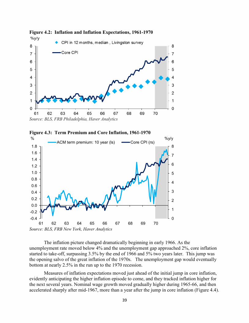
39

Figure 4.2: Inflation and Inflation Expectations, 1961-1970

Source: BLS, FRB Philadelphia, Haver Analytics

Figure 4.3: Term Premium and Core Inflation, 1961-1970

Source: BLS, FRB New York, Haver Analytics

The inflation picture changed dramatically beginning in early 1966. As the unemployment rate moved below 4% and the unemployment gap approached 2%, core inflation started to take-off, surpassing 3.5% by the end of 1966 and 5% two years later. This jump was the opening salvo of the great inflation of the 1970s. The unemployment gap would eventually bottom at nearly 2.5% in the run up to the 1970 recession.

Measures of inflation expectations moved just ahead of the initial jump in core inflation, evidently anticipating the higher inflation episode to come, and they tracked inflation higher for the next several years. Nominal wage growth moved gradually higher during 1965-66, and then accelerated sharply after mid-1967, more than a year after the jump in core inflation (Figure 4.4).

0

1

2

3

4

5

6

7

8

-0.4

-0.2

0.0

0.2

0.4

0.6

0.8

1.0

1.2

1.4

1.6

1.8

61 62 63 64 65 66 67 68 69 70

%y/y%ACM term premium: 10 year (ls) Core CPI (rs)

40

At the same time, productivity growth surged through 1965 as firms evidently found ways to make their existing work force more productive in the face of a tight labor market. This caused unit labor cost inflation to drop briefly into negative territory (Figure 4.5). This dynamic reversed during 1966-67 as productivity growth slowed and unit labor costs accelerated above 4% and eventually significantly higher, no doubt helping to push core inflation higher through the remainder of the decade.

Figure 4.4: Average Hourly Earnings Growth and Inflation, 1965-1969

Source: BLS, Haver Analytics

Figure 4.5: Core Inflation, Unit Labor Cost Growth and Productivity Growth, 1965-1969

Source: BLS, Haver Analytics

1

2

3

4

5

6

7

8

1

2

3

4

5

6

7

8

65 66 67 68 69 70

%y/y%Average hourly earnings (ls) CPI (rs)

-2.5

0.0

2.5

5.0

7.5

10.0

-2.5

0.0

2.5

5.0

7.5

10.0

65 66 67 68 69 70

%%Core CPI

Unit labor costs: non farm business (%y/y)Real output per hour: nonfarm business (%y/y)

41

What caused price and wage inflation and inflation expectations suddenly to shift upward in 1966 after having averaged less than 2% for so many years? Was there really a threshold as the unemployment gap neared 2%? An analysis of the jump in inflation as well as the drop in unemployment may shed some light on this issue. The drop in unemployment reflected growth in aggregate demand (real GDP) that had risen to well above the economy’s 4.5% potential rate of growth at the time. Much of the above-trend GDP growth during this period was fueled by fiscal expansion, including some ongoing effects from the Kennedy tax cuts, and a substantial pickup in both defense spending related to the war in Vietnam and nondefense spending associated with President Johnson’s Great Society programs. An important element of the latter was the introduction of Medicare and Medicaid in the second half of 1965.

The initial surge in inflation in 1965 was broadly based across goods and services; prices for food, shelter, and apparel all accelerated significantly. The single most impressive contributor was health care, where inflation rates more than doubled from already elevated levels over the latter half of the 1960s, led by an even stronger acceleration of physicians’ fees (see Figure 4.6). The Great Society programs were having a substantial impact on the prices of the new services it was providing for. It would take many years for supply in the health care sector to catch up with the government-funded increase in demand. With households suddenly facing surges in prices of such key goods and services, it is little surprise that inflation expectations would finally have become unanchored.

Figure 4.6: PCE Inflation and Medical Care Inflation, 1961-1969

Source: BLS, BEA, Haver Analytics

Monetary policy also played an important part in the unanchoring of inflation expectations and the ongoing rise in inflation in the latter 1960s. The Fed’s initial reaction to the jump in inflation was to tighten policy modestly. Based on a reading of FOMC minutes and staff Greenbook analyses at the time, the FOMC recognized that the economy had moved beyond full employment and that inflation risks were rising. 13 The Committee agreed that its policy should 13 For example, the minutes from the January 11, 1966 FOMC meeting noted that: “Chairman Martin thought the Committee was more or less in agreement on policy… the System now would be operating in an entirely new

0

2

4

6

8

10

0

2

4

6

8

10

63 64 65 66 67 68 69

CPI: medical care services

Personal consumption expenditures: health care price index

PCE exculding food & energy: chain price index

% y/y % y/y

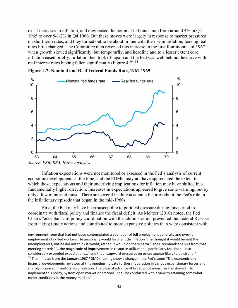
42

resist increases in inflation, and they raised the nominal fed funds rate from around 4% in Q4 1965 to over 5-1/2% in Q4 1966. But these moves were largely in response to market pressures on short term rates, and they turned out to be about in line with the rise in inflation, leaving real rates little changed. The Committee then reversed this increase in the first four months of 1967 when growth slowed significantly, but temporarily, and headline and to a lesser extent core inflation eased briefly. Inflation then took off again and the Fed was well behind the curve with real interest rates having fallen significantly (Figure 4.7).14

Figure 4.7: Nominal and Real Federal Funds Rate, 1961-1969

Source: FRB, BEA, Haver Analytics

Inflation expectations were not monitored or assessed in the Fed’s analysis of current economic developments at the time, and the FOMC may not have appreciated the extent to which those expectations and their underlying implications for inflation may have shifted in a fundamentally higher direction. Increases in expectations appeared to give some warning, but by only a few months at most. There are several leading academic theories about the Fed's role in the inflationary episode that began in the mid-1960s.

First, the Fed may have been susceptible to political pressure during this period to coordinate with fiscal policy and finance the fiscal deficit. As Meltzer (2010) noted, the Fed Chair's "acceptance of policy coordination with the administration prevented the Federal Reserve from taking timely actions and contributed to more expansive policies than were consistent with environment--one that had not been contemplated a year ago--of full employment generally and over-full employment of skilled workers. He personally would favor a little inflation if he thought it would benefit the unemployables, but he did not think it would; rather, it would do them harm.” The Greenbook analysis from that meeting stated: ““…the magnitude of improvement in resource utilization – particularly for labor -- also considerably exceeded expectations…” and that “…upward pressures on prices appear likely to be strong.” 14 The minutes from the January 1967 FOMC meeting show a change in the Fed’s tone: “The economic and financial developments reviewed at this meeting indicate further moderation in various expansionary forces and sharply increased inventory accumulation. The pace of advance of broad price measures has slowed… To implement this policy, System open market operations…shall be conducted with a view to attaining somewhat easier conditions in the money market.”

0

2

4

6

8

10

0

2

4

6

8

10

63 64 65 66 67 68 69 70

%% Nominal fed funds rate Real fed funds rate

43

price stability." Or, as Lacker (2017) put it more colorfully, President Johnson could be very convincing as he drove the Fed Chair around his Texas ranch at breakneck speeds in his white Cadillac.

This was also a time shortly after the famous paper by Paul Samuelson and Robert Solow (1960) was published, in which they argued that policy makers could achieve a “nonperfectionist” goal of a 3% unemployment rate at what they considered to be a tolerable inflation rate of 4 to 5%. This thinking was influential among academic economists, some of whom were in the Kennedy and Johnson administrations, who promoted the adoption of expansionary policies to stimulate the economy and bring inflation down to low levels.

Second, the Fed may have made analytical errors by both overestimating the degree of slack in the economy and underestimating the sensitivity of inflation to slack. For example, Romer and Romer (2002) argue that the implicit estimate of NAIRU that can be inferred from the Fed's Greenbook forecasts during the time was around 2.5%. This compares with the CBO's current estimate of about 5.5% during the mid-1960s. As Powell (2018a) put it, “…policymakers misperceived the level of the natural rate of unemployment, which we now believe had shifted up markedly in the 1960s. With the higher natural rate, the labor market was much tighter and provided much greater upward pressure on inflation than policymakers realized in real time. As a result, they were continually "behind the curve.”

On both counts, we may be better off today than we were a little over 50 years ago, with an emphasis on “may.” With respect to the second issue, we suspect that much has been learned over time on the data front, but uncertainty about concepts like the natural rates of unemployment and interest may be just as high today as they were in the mid 1960s, as suggested by Powell (2018b).

On the political front, the Administration has expressed displeasure with some of its choices for the Board of Governors, and in the past month, the Wall Street Journal reported that top White House economic adviser Lawrence Kudlow said President Trump will seek to fill two Federal Reserve Board vacancies with nominees who don’t believe a rapidly expanding economy has to fuel faster inflation. Kudlow was quoted as saying, “The White House wants highly capable, competent people who understand that you can have strong economic growth without higher inflation. Surges in the economy’s productive capacity mean that more people can work at higher wages without causing inflation to pick up.” If political pressure leads the FOMC to move to a belief that a rapidly expanding economy poses no inflationary dangers, there would be a shift toward policy views that were present in the 1960s.

In sum, there are important parallels and important differences between the 1960s and today.

Parallels:

In both periods the unemployment rate was approaching 3-1/2% from substantially higher levels with little or no evidence of core price inflation rising significantly above the relatively subdued levels they had been at for many years.

Fiscal stimulus was boosting aggregate demand Consistent with low realized inflation, inflation expectations were stuck at low levels.

44

While Fed officials during both periods were/are aware of the effects of tight resource utilization on inflation, the absence of inflation pressures despite steep declines in unemployment led to beliefs that NAIRU was low, and could be falling, and that the Phillips curve was flat

The Fed faced strong political pressure from the Administration not to raise rates Uncertainty about NAIRU remains high

Differences:

The NAIRU was estimated to be considerably higher in the 1960s than it is now; we still have a ways to go to get to an unemployment gap of negative 1.5-2.0%; various technological advances may be reducing the NAIRU even further today.

The Fed’s policy performance since the great inflation and its adoption of a formal price mandate and specific inflation objective in 2012 may have helped to anchor inflation expectations more solidly than they were in the mid-1960s

Today’s Fed has had the benefit of having learned from past experience: o At least until very recently, they have been tightening in a pre-emptive, though

gradual manner, and recognize that the fed funds rate has to rise by more than one-for-one with inflation in order to tighten policy. They are also mindful of the central importance of Fed independence in the conduct of policy.

o But the composition of FOMC membership can change over time.

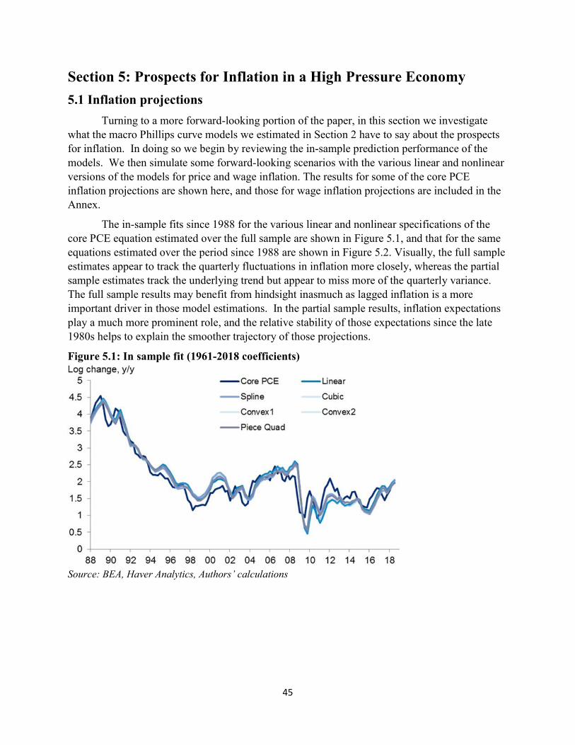
45

Section 5: Prospects for Inflation in a High Pressure Economy

5.1 Inflation projections

Turning to a more forward-looking portion of the paper, in this section we investigate what the macro Phillips curve models we estimated in Section 2 have to say about the prospects for inflation. In doing so we begin by reviewing the in-sample prediction performance of the models. We then simulate some forward-looking scenarios with the various linear and nonlinear versions of the models for price and wage inflation. The results for some of the core PCE inflation projections are shown here, and those for wage inflation projections are included in the Annex.

The in-sample fits since 1988 for the various linear and nonlinear specifications of the core PCE equation estimated over the full sample are shown in Figure 5.1, and that for the same equations estimated over the period since 1988 are shown in Figure 5.2. Visually, the full sample estimates appear to track the quarterly fluctuations in inflation more closely, whereas the partial sample estimates track the underlying trend but appear to miss more of the quarterly variance. The full sample results may benefit from hindsight inasmuch as lagged inflation is a more important driver in those model estimations. In the partial sample results, inflation expectations play a much more prominent role, and the relative stability of those expectations since the late 1980s helps to explain the smoother trajectory of those projections.

Figure 5.1: In sample fit (1961-2018 coefficients)

Source: BEA, Haver Analytics, Authors’ calculations

46

Figure 5.2: In sample fit (1988-2018 coefficients)


In Figure 5.3, we show a similar figure for the models estimated over the full sample, except that the focus here is on the fit during the tight labor market period of the latter 1960s. Whereas during other periods it was difficult to distinguish between the different nonlinear versions, when the labor market tightened significantly, the differences across these models began to show up significantly.

Figure 5.3: In-sample fit over the 1960s (1961-2018 coefficients)


Turning to the projections, we considered two scenarios. In the first scenario, unemployment was assumed to follow the median path in the FOMC’s December 2018 summary

47

of economic projections (SEP). In the second scenario, the unemployment rate is assumed to decline further to 3% by the end of 2020 and remain there through 2021. In both cases, the natural rate or NAIRU was assumed to remain at the FOMC’s median longer run projection of 4.4%. The resulting unemployment gaps are shown in Figure 5.4. Under both scenarios the unemployment gap is negative throughout, but diminishes in the SEP median scenario and declines to and remains at nearly-1.4% in the tighter labor market scenario.

Figure 5.4: Unemployment Gap Scenarios

Source: BLS, CBO, FRB, Haver Analytics, Authors’ calculations

For the price-Phillips curves, inflation expectations were assumed to hold steady at 2% (though this assumption was later relaxed), and relative import prices were held at their 2018Q3 values. Lagged inflation was projected dynamically by each model (i.e., next period’s lagged inflation was the model’s prediction of inflation this period). For the wage equation projections (which are reported in the Annex), inflation expectations and trend productivity growth were held constant at their 2018Q3 values and lagged inflation was handled in two different ways. In one case, lagged inflation was assumed to follow the December 2018 FOMC median projections. In a second case, lagged inflation was assumed to follow the mean projection of the various core PCE inflation models matched by sample period. (In this latter case, for example, lagged inflation for the wage-Phillips curves estimated over the longer sample period from the 1960s to 2018 was assumed to follow the mean projection of the price Phillips curves estimated over the same period.) Finally, in order to consider the possibility of a shift to a nonstationary or adaptive expectations regime, we endogenized inflation expectations, having them move with lagged inflation projections as discussed further below.15

15 We elected not to use the model itself to predict lagged inflation in a rational expectations framework because we wanted to see what would happen if the structure of the model reverted to more of an adaptive expectations framework as existed prior to the 1980s. The projections reported here are partial-equilibrium scenarios designed

48

Figures 5.5 and 5.6 present projections with the core PCE models estimated over the full sample and the more recent sample period respectively; in both cases FOMC median unemployment projections were used. The forecasts of inflation generally dip in the near term because of the lagged effects of the transitory drop in inflation in 2017. Models based on the full sample period show a significant upward trajectory over the next three years, more so for the nonlinear variants—especially the spline equation—than the linear version. This reflects the steeper nonlinear Phillips curve slopes that apply when the unemployment gap is negative. The more recent sample period yields forecasts that are much flatter and more in line with (though still several tenths above) the median FOMC inflation projections.

Figure 5.5: Core PCE Scenario 1: FOMC Median Unemployment Path, 1961-2018 Coefficients

Source: BEA, FRB, Haver Analytics, Authors’ calculations

to show the properties of the different models rather than true forecasts. These projections do not factor in the likely policy reactions that significant increases in inflation would induce.

1.0

1.5

2.0

2.5

3.0

3.5

4.0

4.5

5.0

1.0

1.5

2.0

2.5

3.0

3.5

4.0

4.5

5.0

2016 2017 2018 2019 2020 2021

Core PCE Linear Spline

Cubic Convex1 Convex2

Piece Quad Fed Dec Forecast

%, y/y %, y/y

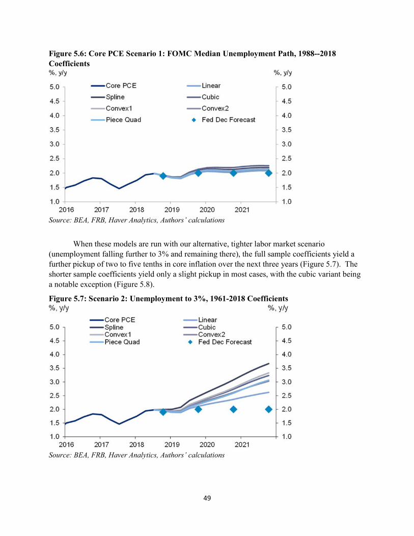
49

Figure 5.6: Core PCE Scenario 1: FOMC Median Unemployment Path, 1988--2018 Coefficients


When these models are run with our alternative, tighter labor market scenario (unemployment falling further to 3% and remaining there), the full sample coefficients yield a further pickup of two to five tenths in core inflation over the next three years (Figure 5.7). The shorter sample coefficients yield only a slight pickup in most cases, with the cubic variant being a notable exception (Figure 5.8).

Figure 5.7: Scenario 2: Unemployment to 3%, 1961-2018 Coefficients


50

Figure 5.8 Scenario 2: Unemployment to 3%, 1988-2018 coefficients


Finally, we considered what would happen if in the event of a further tightening of the labor market to 3% unemployment, inflation expectations shifted away from being anchored at 2% (as we have assumed in all of the projection scenarios so far) and instead became more adaptive. To achieve this effect, we estimated an equation for inflation expectations as a function of lagged inflation over the adaptive expectations period from the mid- 1960s to the early 1980s. Our specific model, using three lags on inflation was:

𝜋 = 0.63 + 0.30𝜋 + 0.02𝜋 + 0.34𝜋

based on data for the period 1964Q1 – 1981Q4.

Allowing inflation expectations to adjust away from a 2% anchor, albeit slowly, moves the inflation outcomes up noticeably further (Figure 5.9). The increase is considerably more subdued under the more recent sample estimation (Figure 5.10). If unemployment were to decline to 3% and remain there for a couple years, the full-sample results might be more pertinent than the post-1988 sample results, because a period of such tight labor markets could be enough to begin to shift the current very stationary Phillips curve into a more nonstationary regime as in Nalewaik’s work and the experience of the 1960s suggested. That is, inflation expectations would become more adaptive, inflation more persistent, and the Phillips curve steeper, as captured in the full sample coefficients. Were such a shift to occur, the various projections in Figure 5.15 say that inflation could rise to between 2.75% (linear model) and 4.25% (spline model) over the next three years in the event of the tighter labor market scenario. Of course, it is unlikely that inflation would rise as much as some of these model projections suggest over this time period, because the Fed would most likely step in with policy restraint if it became evident that inflation expectations were becoming unmoored.

51

Figure 5.9: Scenario 2: Unemployment goes to 3%, 1961-2018 Coefficients


Figure 5.10: Scenario 2: Unemployment goes to 3%, 1988-2018 Coefficients


52

Section 6. Conclusions As the USMPF gathers this year, belief that the Phillips curve is dead has never been stronger, at least not for the past 50 years. Unemployment has been running noticeably below most estimates of the natural rate for well over a year now, while core inflation has remained persistently below the Fed’s objective.

The Fed has moved essentially to neutral recently despite unemployment continuing to run noticeably below its estimate of NAIRU with ample momentum behind it, partly because of growing risks to the outlook abroad, but partly also because of concern that inflation remains slightly below 2% despite a seemingly tight labor market. Doubts about the Phillips curve relationship may well be on the rise even within the Fed.

Evidence that the price Phillips curve has been dormant for the past several decades does not necessarily mean that it is dead. As the empirical evidence in this paper indicates, the Phillips curve could be hibernating, and there is a risk of the Phillips curve waking up, with inflationary pressures rising in the face of an overheating labor market.

There are several arguments from the evidence in this paper that we can have concerns about inflation if we continue to experience a high-pressure economy.

First, some of our empirical specifications in Section 2 of the paper, suggest that the price-Phillips curve might have substantial nonlinearities. If these nonlinearities are present, the simulations in Section 5 suggest that inflation could rise above the Fed’s target level if the unemployment rate continues on the path projected in December by the FOMC participants, or declines even further. However, the evidence from the post-1988 sample period is much less supportive of these nonlinearities. We are not sure which Phillips curve sample periods provides more reliable information about where the Phillips curve is now. However, the state and MSA evidence suggests that the post-1988 Phillips curve may not be able to reveal these nonlinearities because there are so few observations of very tight labor markets since 1988 and possibly because of the endogoneity of monetary policy. The state and MSA data, which has many more observations with very tight labor markets, suggests that the Phillips curve with nonlinearities might be alive and well. Thus the reports of the death of the Phillips curve might be greatly exaggerated. We should not discount the possibility that substantial nonlinearities are present in today’s Phillips curve and so a high-pressure economy could lead to inflationary pressures.

Second, our evidence, both in the macro, time-series data and the state and MSA data in Sections 4 and 5, suggests that the wage-Phillips curve is alive and well. This is consistent with the observation that wage inflation has marched steadily, if slowly, upward in recent years as the labor market has tightened, as shown in Figure 6.1. However, Chair Powell (2018b) has noted, we did see something like this in the late 1990s-early 2000s without an inflation lift (Figure 6.2). But that was also a period during with strong dollar helped keep a tight lid on inflation, and the tight labor market was cut short by the recession of 2001, Could we see this play out again? Wage inflation did rise significantly in the late 90s (both in nominal terms and in excess of productivity trends), as it had in the mid 1960s. While the wage Phillips curve may have flattened some over time, it remains much steeper and evidence of nonlinearities much more robust than for the price Phillips curve in the post-1988 sample period. It is possible that the link between wage and price inflation has become weak, but this is a puzzle that requires further research.

53

Figure 6.1: Unemployment Gap and Wage Growth, 2008-2016

Source: BLS, CBO, Haver Analytics Figure 6.2: Unemployment Gap and Wage Growth, 1992-2002


Third, Nalewaik’s (2016) evidence suggests that the economy can switch from a stationary regime, in which shocks to inflation only have transitory effects on inflation and inflation expectations are anchored, to a nonstationary regime, in which shocks to inflation have persistent effects and inflation expectations become unanchored. Our case study of the 1960s in Section 4 and the parallels between that period and the current one suggest that there is a possibility that we could move to a nonstationary regime if the unemployment rate stays well

0.5

1.0

1.5

2.0

2.5

3.0

3.5

4.0

-1

0

1

2

3

4

5

08 09 10 11 12 13 14 15 16 17 18 19

Unemployment gap (ls)Avg hourly earnings: prod & nonsupervisory: total pvt industries (rs)Employment cost index: civilian workers (rs)Core PCE (rs)

% % y/y

0.5

1.0

1.5

2.0

2.5

3.0

3.5

4.0

4.5

5.0

-2

-1

0

1

2

3

92 93 94 95 96 97 98 99 00 01 02

Unemployment gap (ls)

Avg hourly earnings: prod & nonsupervisory: total pvt industries (rs)

Employment cost index: civilian workers (rs)

Core PCE (rs)

% % y/y

54

below the natural rate of unemployment for a long period of time, especially if political pressures begin to influence market expectations. We do not think this is a likely scenario because starting in 2012, the Federal Reserve has adopted the monetary policy strategy of inflation targeting which has proved successful in anchoring inflation expectations in many countries. However, changes in the composition of the FOMC could possibly weaken the Fed’s commitment to its inflation target, which would make an unmooring of inflation expectations more likely. If inflation expectations did become unanchored, our case study of the 1960s in Section 4 and the simulations in Section.5 do raise concerns that inflation could become a problem.

We want to be very clear that the evidence in this paper does not say that inflation will rise in the near future. First, our evidence is ambiguous about the degree to which the Phillips curve may have a steeper slope and nonlinearities because we obtain different results for the pre-1988 and post-1988 sample period. However, because of the lack of variation in the unemployment gap data since 1988 and the endogeneity of monetary policy in this sample period, we are more doubtful that the 1988-2018 estimated Phillips curve is reliable. Second, there is currently substantial uncertainty about whether the economy will remain in a high-pressure mode. Thus our analysis not about whether inflation will rise in the near future, but rather that we cannot be complacent about inflationary pressures. As we have discussed, the flattening of the Phillips curve in recent decades reflects some combination of the absence of very tight labor markets, the endogeneity bias of monetary policy, and the anchoring of inflation expectations. Monetary policy committed to stabilizing inflation has been central to all three of these factors. A departure from this policy would likely lead to a steepening of the Phillips curve.

55

References

Adrian, Tobias, Richard K. Crump, and Emanuel Moench, "Pricing the Term Structure with Linear Regressions," Journal of Financial Economics 110, no. 1 (October 2013): 110-138.

Babb, Nathan R. and Alan K. Detmeister (2017). "Nonlinearities in the Phillips Curve for the United States : Evidence Using Metropolitan Data," Finance and Economics Discussion Series 2017-070, Board of Governors of the Federal Reserve System.

Ball, Laurence M., and Sandeep Mazumder (2011). “Inflation Dynamics and the Great Recession”, National Bureau of Economic Research, Working Paper no. 17044.

Barnes, Michelle L. and Giovanni P. Olivei (2003). “Inside and Outside the Bounds: Threshold Estimates of the Phillips Curve,” Federal Reserve Bank of Boston New England Economic Review, 3-18.

Bernanke, Ben S. (2007). "Inflation Expectations and Inflation Forecasting," speech delivered at the Monetary Economics Workshop of the National Bureau of Economic Research Summer Institute, Cambridge, Mass., July 10, 2007.

Blanchard, Olivier (2016). "The U.S. Phillips Curve: Back to the 60s? " Policy Brief Number PB16-1. Washington: Peterson Institute for International Economics.

Brayton, Flint, John M. Roberts, and John C. Williams (1999). “What's Happened to the Phillips Curve?” Finance and Economics Discussion Series 99-49, Board of Governors of the Federal Reserve System.

Chodorow-Reich, Gabriel (forthcoming). "Geographic Cross-Sectional Fiscal Spending Multipliers: What Have We Learned?." American Economic Journal: Economic Policy.

Cecchetti, Stephen G., Michael E. Feroli, Peter Hooper, Anil K Kashyap, and Kermit L. Schoenholtz (2017). “Deflating Inflation Expectations: The Implications of Inflation’s Simple Dynamics,” US Monetary Policy Forum.

Daly, Mary C. and Bart Hobjin (2014). “Downward Nominal Wage Rigidities Bend the Phillips Curve,” Journal of Money, Credit and Banking, September 23, 2014.

Daly, Mary C., Bart Hobijn, and Benjamin Pyle (2016). “What’s Up with Wage Growth?”, Federal Reserve Bank of San Francisco Economic Letter 2016-07, March 7.

Doser, Alexander, Ricardo C. Nunes, Nikhil Rao and Viacheslav Sheremirov (2017). “Inflation Expectations and Nonlinearities in the Phillips Curve”, Federal Reserve Bank of Boston, Working Paper no. 17-11.

Fitzgerald, Terry J., and Juan Pablo Nicolini (2014). “Is there a Stable Relationship Between Unemployment and Future Inflation? Evidence from U.S. Cities,” Federal Reserve Bank of Minneapolis Research Department Working Paper 713, May.

Guren, Adam, Alisdair McKay, Emi Nakamura, and Jon Steinsson (2018). “What Do We Learn From Cross-Sectional Empirical Estimates in Macroeconomics?” mimeo.

Michael T. Kiley (2008). "Monetary policy actions and long-run inflation expectations," Finance and Economics Discussion Series 2008-03, Board of Governors of the Federal Reserve System.

56

Kiley, Michael T. (2015). "Low Inflation in the United States: A Summary of Recent Research," FEDS Notes. Board of Governors of the Federal Reserve System.

Kozicki, Sharon and Peter Tinsley (2001). “Term Structure Views of Monetary Policy under Alternative Models of Agent Expectations.” Journal of Economic Dynamics & Control, January, 149-84.

Kumar, Anil and Pia M. Orrenius (2016). "A closer look at the Phillips curve using state-level data," Journal of Macroeconomics, Elsevier, vol. 47(PA), pages 84-102.

Lacker, Jeffrey M (2017). Comments on “Inflation Dynamics in Stable and Unstable Policy Regimes: Comment on 'Deflating Inflation Expectations'” US Monetary Policy Forum, New York, March 3, 2017.

Leduc, Sylvain, Chitra Marti, and Daniel J. Wilson (2019), “Does Ultra-Low Unemployment Spur Rapid Wage Growth” Federal Reserve Bank of San Francisco Economic Letter, January 14.

Leduc, Sylvain and Daniel J. Wilson (2017). “Has the Wage Phillips Curve Gone Dormant?,” Federal Reserve Bank of San Francisco Economic Letter, October 16, 2017.

Luzzetti, Matthew, Peter Hooper, Francis Yared, and Laura Desplans, (2017). “Trapped in a low inflation expectations regime? Lessons from the 60s and 80s.” Deutsche Bank Economic Research Special Report, June 23.

McLeay, Michael and Silvana Tenreyro (2018). “Optimal Inflation and the Identification of the Phillips Curve,” manuscript, April.

Meltzer, Allan H., (2010). A History of the Federal Reserve: Volume 2, Chicago: University of Chicago Press

Mishkin, Frederic S. (2007). "Inflation Dynamics," International Finance Vol. 10, No. 3: 317-334.

Mishkin, Frederic S. (2011) “Monetary Policy Strategy: Lessons From the Crisis” in Marek Jarocinski, Frank Smets and Christian Thimann, eds. Monetary Policy Revisited: Lessons from the Crisis, Sixth ECB Central Banking Conference (European Central Bank: Frankfurt): 67-118

Murphy, Anthony. (2018). “The Death of the Phillips Curve?”, Federal Reserve Bank of Dallas, Working Paper 1801, January.

Nalewaik, Jeremy (2016). “Non-Linear Phillips Curves with Inflation Regime-Switching”, Finance and Economics Discussion Series 2016-078. Washington: Board of Governors of the Federal Reserve System

Ng, Wessel, and Sheiner (2018). “The Hutchins Center Explains: The Phillips Curve”, Brookings, August 21.

Orphanides, Athanasios and John C. Williams (2013). "Monetary Policy Mistakes and the Evolution of Inflation Expectations," NBER Chapter in: The Great Inflation: The Rebirth of Modern Central Banking, pages 255-288 National Bureau of Economic Research, Inc.

Peach, Richard W., Robert W. Rich, and Anna Cororaton (2011). “How Does Slack Influence Inflation?”, Federal Reserve Bank of New York, Current issues in economics and finance, Volume 17, Number 3201

57

Pfajfar, Damjan, and John M. Roberts (2018). "The Role of Expectations in Changed Inflation Dynamics," Finance and Economics Discussion Series 2018-062. Board of Governors of the Federal Reserve System.

Phillips, A. W. (1958). “The Relationship between Unemployment and the Rate of Change of Money Wages in the United Kingdom, 1861-1957.” Economica 25, no. 100: 283-99.

Powell, Jerome (2018a). “Monetary Policy and Risk Management at a Time of Low Inflation and Low Unemployment”, Speech at the "Revolution or Evolution? Reexamining Economic Paradigms" 60th Annual Meeting of the National Association for Business Economics, Boston, Massachusetts, October 2, 2018

Powell, Jerome (2018b). "Monetary Policy in a Changing Economy," Speech delivered at "Changing Market Structure and Implications for Monetary Policy," a symposium sponsored by the Federal Reserve Bank of Kansas City, Jackson Hole, Wyoming, August 24, 2018.

Roberts, John M. (2006). “Monetary Policy and Inflation Dynamics,” International Journal of Central Banking, vol. 2, no. 3, pp 193-230.

Romer, Christina D. and David H. Romer (2002). “The evolution of economic understanding and postwar stabilization policy”, National Bureau of Economic Research, Working Paper no. 9274, October, 2002.

Samuelson, Paul and Robert Solow (1960). “Analytical Aspecs of Anti-Inflation Policy,” American Economic Review 50 (Papers and Proceedings): 177-194.

Stock, James, and Mark Watson (2007). "Why Has U.S. Inflation Become Harder to Forecast?", Journal of Money, Credit, and Banking, vol. 39 (February), pp. 3-33.

Stock, James, and Mark Watson. (2009). “Phillips Curve Inflation Forecasts.” In Understanding Inflation and the Implications for Monetary Policy: A Phillips Curve Retrospective. Proceedings of the Federal Reserve Bank of Boston’s 2008 economic conference. Cambridge, Mass.: MIT Press.

Tobin, James (1972) “Inflation and Unemployment,” American Economic Review, vol. 62, no 1, March 1972, pp 1-18.

Yellen, Janet L. (2015). "Inflation Dynamics and Monetary Policy," Speech at the Philip Gamble Memorial Lecture, University of Massachusetts, Amherst, September 24, 2015.

Yellen, Janet L (2017). "Inflation, Uncertainty, and Monetary Policy," Speech delivered at "Prospects for Growth: Reassessing the Fundamentals," 59th Annual Meeting of the National Association for Business Economics, Cleveland, Ohio, September 26, 2017.

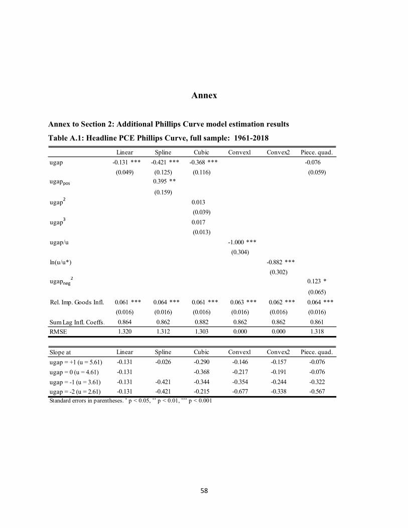
58

Annex

Annex to Section 2: Additional Phillips Curve model estimation results

Table A.1: Headline PCE Phillips Curve, full sample: 1961-2018

ugap -0.131 *** -0.421 *** -0.368 *** -0.076

ugappos 0.395 **

ugap2 0.013

ugap3 0.017

ugap/u -1.000 ***

ln(u/u*) -0.882 ***

ugapneg2 0.123 *



RMSE

Slope at

ugap = +1 (u = 5.61)

ugap = 0 (u = 4.61)

ugap = -1 (u = 3.61)



-0.131

-0.131

-0.131

-0.131

-0.421

-0.421

-0.026 -0.290

-0.338

-0.244

-0.191

-0.157

-0.677

-0.354

-0.217

-0.146

-0.215

-0.344

-0.368


1.318

-0.567

-0.322

-0.076

-0.076

Piece. quad.

0.862

1.320 1.312 1.303 0.000 0.000

(0.016)

0.864 0.862 0.882 0.862

(0.016)

0.861

(0.059)(0.116)(0.125)(0.049)

(0.159)

(0.039)

(0.013)

(0.304)

(0.302)

(0.065)

(0.016)(0.016)(0.016)(0.016)

59

Table A.2: Headline PCE Phillips Curve, extended sample: 1949-2018

ugap -0.057 -0.083 -0.192 -0.083

ugappos 0.039

ugap2

-0.042

ugap3

0.020

ugap/u -0.245

ln(u/u*) -0.301

ugapneg2 -0.042



RMSE

Slope at

ugap = +1 (u = 5.61)

ugap = 0 (u = 4.61)

ugap = -1 (u = 3.61)


0.086

0.001

-0.083

-0.083


-0.217

-0.115

-0.083

-0.065

-0.054

Piece. quad.

-0.057

-0.057

-0.057

-0.057

-0.083

-0.083

-0.044

-0.166

-0.087

-0.053

-0.036

0.212

-0.048

-0.192


(0.051) (0.145) (0.125) (0.073)

(0.198)

(0.058)

(0.018)

(0.312)

(0.310)

(0.087)

(0.016)

0.825 0.824 0.839 0.823 0.824 0.826

(0.016) (0.016) (0.016) (0.016) (0.016)

1.5541.552 1.555 1.552 1.553 0.000

60

Table A.3: Wage Phillips Curve (Compensation per Hour): 1964-2018

ugap -0.386 *** -0.847 *** -0.710 *** -0.300

ugappos 0.606 *

ugap2

0.029

ugap3

0.019

ugap/u -2.678 ***

ln(u/u*) -2.498 ***

ugapneg2 -0.206

Trend prod. growth. 0.671 ** 0.591 ** 0.525 * 0.603 ** 0.626 ** 0.641 **

RMSE

Slope at

ugap = +1 (u = 5.61)

ugap = 0 (u = 4.61)

ugap = -1 (u = 3.61)


2.7662.767 2.761 2.763 2.758 2.763

(0.138)

(0.285) (0.287) (0.282) (0.283) (0.283) (0.286)

(0.149) (0.247) (0.269) (0.182)

(0.356)

-0.386

-0.386

-0.386

-0.386

-0.847

-0.847

-0.240

0.524

0.112

-0.300

-0.300

-0.603

-0.712

-0.710

-0.595

-1.812

-0.947

-0.581

-0.392

Cubic Convex1

-0.957

-0.692

-0.542

-0.445

(0.094)

(0.030)

(0.798)

(0.883)



Linear Spline

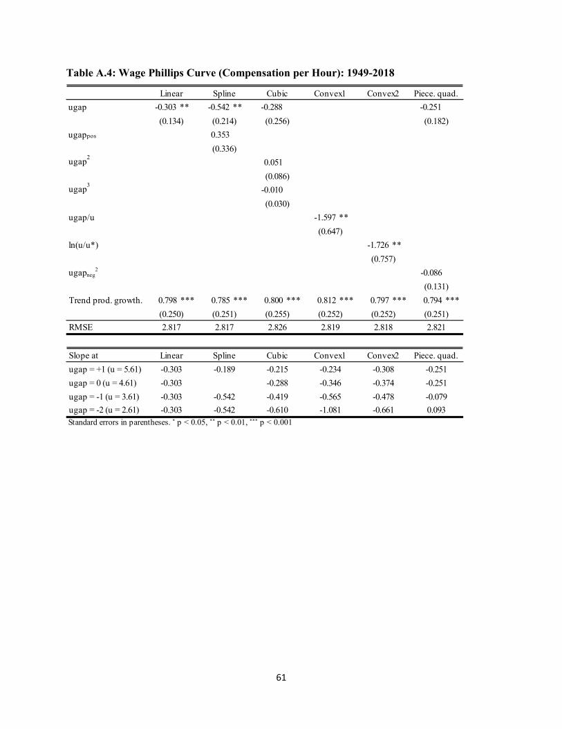
61

Table A.4: Wage Phillips Curve (Compensation per Hour): 1949-2018

ugap -0.303 ** -0.542 ** -0.288 -0.251

ugappos 0.353

ugap2

0.051

ugap3

-0.010

ugap/u -1.597 **

ln(u/u*) -1.726 **

ugapneg2 -0.086

Trend prod. growth. 0.798 *** 0.785 *** 0.800 *** 0.812 *** 0.797 *** 0.794 ***

RMSE

Slope at

ugap = +1 (u = 5.61)

ugap = 0 (u = 4.61)

ugap = -1 (u = 3.61)


2.817 2.817 2.826 2.819 2.818

(0.250) (0.251) (0.255) (0.252) (0.252)

(0.336)

(0.086)

(0.030)

(0.647)

(0.757)


(0.134) (0.214) (0.256)


0.093

-0.079

-0.251

-0.251

Piece. quad.

(0.182)

(0.131)

(0.251)

2.821

-0.346

-0.234

-0.661

-0.478

-0.374

-0.308


-0.303

-0.303

-0.303

-0.303

-0.542

-0.542

-0.189

-0.610

-0.419

-0.288

-0.215

-1.081

-0.565

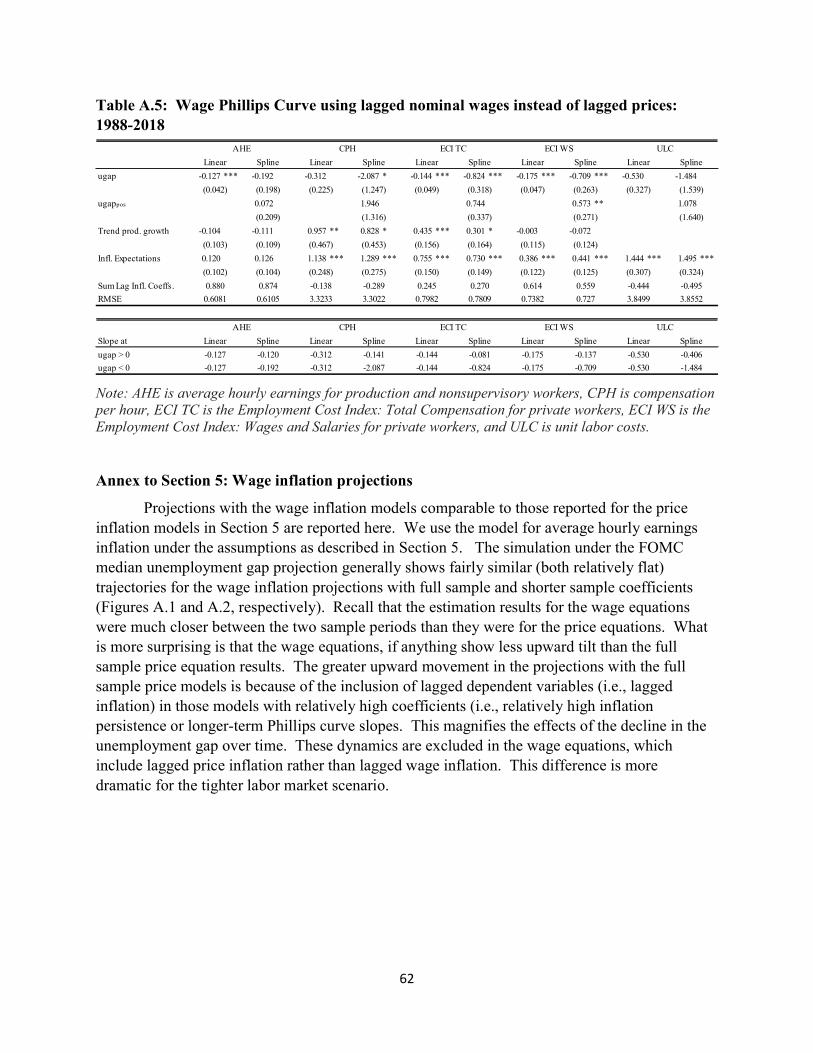
62

Table A.5: Wage Phillips Curve using lagged nominal wages instead of lagged prices: 1988-2018

Note: AHE is average hourly earnings for production and nonsupervisory workers, CPH is compensation per hour, ECI TC is the Employment Cost Index: Total Compensation for private workers, ECI WS is the Employment Cost Index: Wages and Salaries for private workers, and ULC is unit labor costs.

Annex to Section 5: Wage inflation projections

Projections with the wage inflation models comparable to those reported for the price inflation models in Section 5 are reported here. We use the model for average hourly earnings inflation under the assumptions as described in Section 5. The simulation under the FOMC median unemployment gap projection generally shows fairly similar (both relatively flat) trajectories for the wage inflation projections with full sample and shorter sample coefficients (Figures A.1 and A.2, respectively). Recall that the estimation results for the wage equations were much closer between the two sample periods than they were for the price equations. What is more surprising is that the wage equations, if anything show less upward tilt than the full sample price equation results. The greater upward movement in the projections with the full sample price models is because of the inclusion of lagged dependent variables (i.e., lagged inflation) in those models with relatively high coefficients (i.e., relatively high inflation persistence or longer-term Phillips curve slopes. This magnifies the effects of the decline in the unemployment gap over time. These dynamics are excluded in the wage equations, which include lagged price inflation rather than lagged wage inflation. This difference is more dramatic for the tighter labor market scenario.

ugap -0.127 *** -0.192 -0.312 -2.087 * -0.144 *** -0.824 *** -0.175 *** -0.709 *** -0.530 -1.484

ugappos 0.072 1.946 0.744 0.573 ** 1.078

Trend prod. growth -0.104 -0.111 0.957 ** 0.828 * 0.435 *** 0.301 * -0.003 -0.072

Infl. Expectations 0.120 0.126 1.138 *** 1.289 *** 0.755 *** 0.730 *** 0.386 *** 0.441 *** 1.444 *** 1.495 ***


RMSE

Slope at

ugap > 0

ugap < 0

0.559 -0.444 -0.495

(0.042) (0.198)

(0.209)

(0.103) (0.109)

(0.102) (0.104)

0.880 0.874 -0.138 -0.289 0.245 0.270 0.614

(0.124)

(0.248) (0.275) (0.150) (0.149) (0.122) (0.125) (0.307) (0.324)

(0.467) (0.453) (0.156) (0.164) (0.115)

(0.263) (0.327) (1.539)

(1.316) (0.337) (0.271) (1.640)

(0.225) (1.247) (0.049) (0.318) (0.047)

-0.127 -0.192

AHE

Linear Spline

-0.127 -0.120

AHE

Linear Spline

0.6081 0.6105


SplineLinearSplineLinearSplineLinearSplineLinear

3.8499 3.8552

Linear Spline Linear

3.3233 3.3022 0.7982 0.7382 0.727

-0.312 -0.141 -0.144 -0.081

0.7809

-0.406

-0.530 -1.484


Linear Spline Linear Spline

-0.312 -2.087 -0.144 -0.824

Spline

-0.175 -0.137

-0.175 -0.709

-0.530

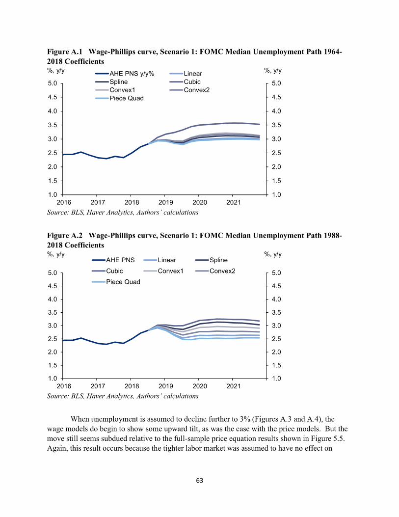
63

Figure A.1 Wage-Phillips curve, Scenario 1: FOMC Median Unemployment Path 1964-2018 Coefficients

Source: BLS, Haver Analytics, Authors’ calculations

Figure A.2 Wage-Phillips curve, Scenario 1: FOMC Median Unemployment Path 1988-2018 Coefficients


When unemployment is assumed to decline further to 3% (Figures A.3 and A.4), the wage models do begin to show some upward tilt, as was the case with the price models. But the move still seems subdued relative to the full-sample price equation results shown in Figure 5.5. Again, this result occurs because the tighter labor market was assumed to have no effect on

1.0

1.5

2.0

2.5

3.0

3.5

4.0

4.5

5.0

1.0

1.5

2.0

2.5

3.0

3.5

4.0

4.5

5.0

2016 2017 2018 2019 2020 2021

AHE PNS y/y% LinearSpline CubicConvex1 Convex2Piece Quad

%, y/y %, y/y

1.0

1.5

2.0

2.5

3.0

3.5

4.0

4.5

5.0

1.0

1.5

2.0

2.5

3.0

3.5

4.0

4.5

5.0

2016 2017 2018 2019 2020 2021

AHE PNS Linear Spline


Piece Quad

%, y/y %, y/y

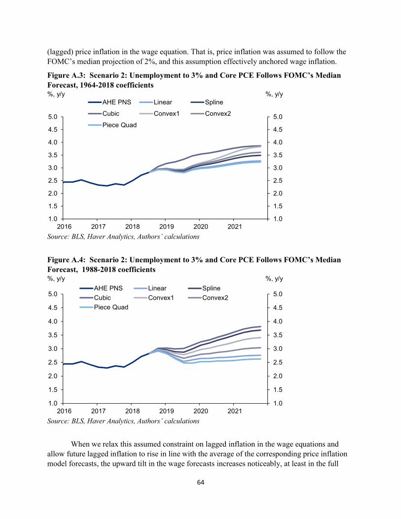
64

(lagged) price inflation in the wage equation. That is, price inflation was assumed to follow the FOMC’s median projection of 2%, and this assumption effectively anchored wage inflation.

Figure A.3: Scenario 2: Unemployment to 3% and Core PCE Follows FOMC’s Median Forecast, 1964-2018 coefficients


Figure A.4: Scenario 2: Unemployment to 3% and Core PCE Follows FOMC’s Median Forecast, 1988-2018 coefficients


When we relax this assumed constraint on lagged inflation in the wage equations and allow future lagged inflation to rise in line with the average of the corresponding price inflation model forecasts, the upward tilt in the wage forecasts increases noticeably, at least in the full

1.0

1.5

2.0

2.5

3.0

3.5

4.0

4.5

5.0

1.0

1.5

2.0

2.5

3.0

3.5

4.0

4.5

5.0

2016 2017 2018 2019 2020 2021



Piece Quad

%, y/y %, y/y

1.0

1.5

2.0

2.5

3.0

3.5

4.0

4.5

5.0

1.0

1.5

2.0

2.5

3.0

3.5

4.0

4.5

5.0

2016 2017 2018 2019 2020 2021



Piece Quad

%, y/y %, y/y

65

sample model projections (Figure 5A.5). The impact in the full sample results is more noticeably than in the post-1988 sample results (Figure A.6) because the corresponding price inflation forecasts rise faster in this scenario (compare Figures 5.7 and 5.8).

Figure A.5: Core PCE Follows Average of Core PCE Forecasts in the 3% Unemployment Scenarios Above, 1964-2018 Coefficients


Figure A.6: Core PCE Follows Average of Core PCE Forecasts in the 3% Unemployment Scenarios Above, 1988-2018 Coefficients


1.0

1.5

2.0

2.5

3.0

3.5

4.0

4.5

5.0

1.0

1.5

2.0

2.5

3.0

3.5

4.0

4.5

5.0

2016 2017 2018 2019 2020 2021



Piece Quad

%, y/y %, y/y

1.0

1.5

2.0

2.5

3.0

3.5

4.0

4.5

5.0

1.0

1.5

2.0

2.5

3.0

3.5

4.0

4.5

5.0

2016 2017 2018 2019 2020 2021



Piece Quad

%, y/y %, y/y

NBER WORKING PAPER SERIES · [email protected] î 6hfwlrq ,qwurgxfwlrq 6wduwlqj lq 0dufk...

Documents

Transcript of NBER WORKING PAPER SERIES · [email protected] î 6hfwlrq ,qwurgxfwlrq 6wduwlqj lq 0dufk...