Navigator GPS Receiver for Fast Acquisition and Weak Signal Space Applications

Presented at the ION GNSS Meeting, Long Beach, CA, September 21-24, 2004. 1

Navigator GPS Receiver for Fast Acquisition and

Weak Signal Space Applications

Luke Winternitz, Michael Moreau, Gregory J. Boegner, Jr. NASA Goddard Space Flight Center Steve Sirotzky, QSS Group, Inc.

BIOGRAPHY Luke Winternitz is an Electrical Engineer in the Hardware Components and Systems Branch at NASA’s Goddard Space Flight Center. He has worked at Goddard for three years primarily in the development of GPS receiver technology. He received Bachelors degrees in Electrical Engineering and Mathematics from the University of Maryland, College Park in 2001 and is currently a part-time graduate student there pursuing a Ph.D. Steve Sirotzky is an Electrical Engineer contracted to the Hardware Components and Systems Branch at NASA's Goddard Space Flight Center. He received his B.S. in Electrical and Computer Engineering from Carnegie Mellon in 1995. Steve spent three years at Qualcomm working on a low earth orbit CDMA based cellular phone system, and another four years at Torrent Networking Technologies/Ericsson IP Infrastructure designing Internet Routers before joining the NASA team. Michael Moreau is an Aerospace Engineer in the Flight Dynamics Analysis Branch at NASA’s Goddard Space Flight Center. His research is focused on applications of the Global Positioning System to enable autonomous navigation and formation flying of spacecraft, and the design of GPS receivers for use in high altitude orbits. He holds a Ph.D. from the University of Colorado, and currently serves as Space Representative on the ION Council. Gregory J. Boegner, Jr. is a senior Electrical Engineer in the Hardware Components and Systems Branch at NASA’s Goddard Space Flight Center. He has over 18 years experience designing analog and digital systems in the fields of communications, embedded control, and digital signal processing. Greg has worked for the U.S. Department of Defense, ASRC Aerospace Corporation, and as an independent consultant. He has a Bachelor of Science Degree in Electrical Engineering from Drexel University in Philadelphia.

ABSTRACT NASA Goddard Space Flight Center (GSFC) is developing a new space-borne GPS receiver that can operate effectively in the full range of Earth orbiting missions from Low Earth Orbit (LEO) to geostationary and beyond [1]. Navigator is designed to be a fully space flight qualified GPS receiver optimized for fast signal acquisition and weak signal tracking. The fast acquisition capabilities provide exceptional time to first fix performance (TTFF) with no a priori receiver state or GPS almanac information, even in the presence of high Doppler shifts present in LEO (or near perigee in highly eccentric orbits). The fast acquisition capability also makes it feasible to imp lement extended correlation intervals and therefore significantly reduce Navigator’s acquisition threshold. This greatly improves GPS observability when the receiver is above the GPS constellation (and satellites must be tracked from the opposite side of the Earth) by providing at least 10 dB of increased acquisition sensitivity. Fast acquisition and weak signal tracking algorithms have been implemented and validated on a hardware development board. A fully functional version of the receiver, employing most of the flight parts, with integrated navigation software is expected by mid 2005. An ultimate goal of this project is to license the Navigator design to an industry partner who will then market the receiver as a commercial product.

INTRODUCTION GPS has found wide application for precision spacecraft navigation and formation flying applications in low Earth orbits (LEO), but recent advances in GPS receiver designs and signal processing capabilities now make it feasible to consider using GPS to provide autonomous, onboard navigation capabilities for geostationary (GEO) or other high altitude space missions. The Geostationary Operational Environmental Satellite (GOES) Program provides one example of a program that would derive significant benefits from a GPS receiver capable of autonomously determining satellite position to 100 meters or less in a GEO orbit; however, options are extremely limited for procuring a receiver that could provide both


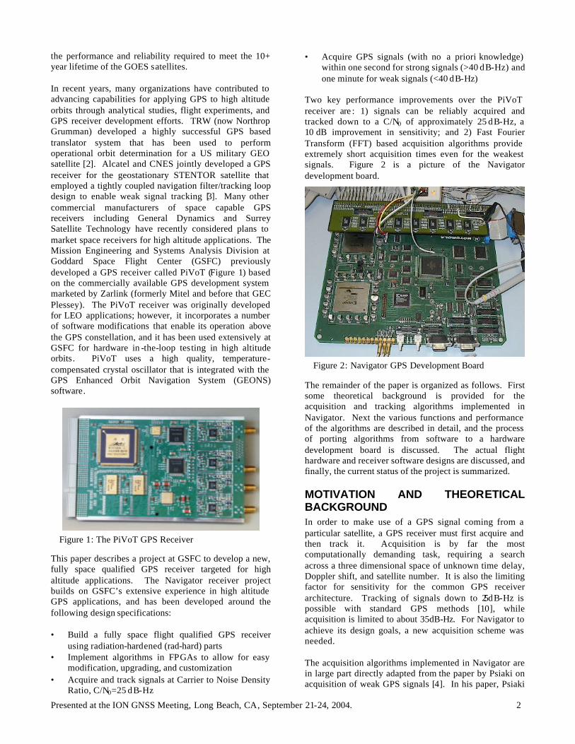
the performance and reliability required to meet the 10+ year lifetime of the GOES satellites. In recent years, many organizations have contributed to advancing capabilities for applying GPS to high altitude orbits through analytical studies, flight experiments, and GPS receiver development efforts. TRW (now Northrop Grumman) developed a highly successful GPS based translator system that has been used to perform operational orbit determination for a US military GEO satellite [2]. Alcatel and CNES jointly developed a GPS receiver for the geostationary STENTOR satellite that employed a tightly coupled navigation filter/tracking loop design to enable weak signal tracking [3]. Many other commercial manufacturers of space capable GPS receivers including General Dynamics and Surrey Satellite Technology have recently considered plans to market space receivers for high altitude applications. The Mission Engineering and Systems Analysis Division at Goddard Space Flight Center (GSFC) previously developed a GPS receiver called PiVoT (Figure 1) based on the commercially available GPS development system marketed by Zarlink (formerly Mitel and before that GEC Plessey). The PiVoT receiver was originally developed for LEO applications; however, it incorporates a number of software modifications that enable its operation above the GPS constellation, and it has been used extensively at GSFC for hardware in -the-loop testing in high altitude orbits. PiVoT uses a high quality, temperature-compensated crystal oscillator that is integrated with the GPS Enhanced Orbit Navigation System (GEONS) software.

Figure 1: The PiVoT GPS Receiver

This paper describes a project at GSFC to develop a new, fully space qualified GPS receiver targeted for high altitude applications. The Navigator receiver project builds on GSFC’s extensive experience in high altitude GPS applications, and has been developed around the following design specifications: • Build a fully space flight qualified GPS receiver

using radiation-hardened (rad-hard) parts • Implement algorithms in FPGAs to allow for easy

modification, upgrading, and customization • Acquire and track signals at Carrier to Noise Density

Ratio, C/N0=25 dB-Hz

• Acquire GPS signals (with no a priori knowledge) within one second for strong signals (>40 dB-Hz) and one minute for weak signals (<40 dB-Hz)

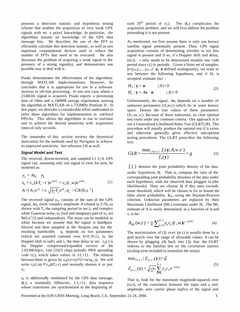
Two key performance improvements over the PiVoT receiver are : 1) signals can be reliably acquired and tracked down to a C/N0 of approximately 25 dB-Hz, a 10 dB improvement in sensitivity; and 2) Fast Fourier Transform (FFT) based acquisition algorithms provide extremely short acquisition times even for the weakest signals. Figure 2 is a picture of the Navigator development board.

Figure 2: Navigator GPS Development Board

The remainder of the paper is organized as follows. First some theoretical background is provided for the acquisition and tracking algorithms implemented in Navigator. Next the various functions and performance of the algorithms are described in detail, and the process of porting algorithms from software to a hardware development board is discussed. The actual flight hardware and receiver software designs are discussed, and finally, the current status of the project is summarized.

MOTIVATION AND THEORETICAL BACKGROUND In order to make use of a GPS signal coming from a particular satellite, a GPS receiver must first acquire and then track it. Acquisition is by far the most computationally demanding task, requiring a search across a three dimensional space of unknown time delay, Doppler shift, and satellite number. It is also the limiting factor for sensitivity for the common GPS receiver architecture. Tracking of signals down to 25dB-Hz is possible with standard GPS methods [10], while acquisition is limited to about 35dB-Hz. For Navigator to achieve its design goals, a new acquisition scheme was needed. The acquisition algorithms implemented in Navigator are in large part directly adapted from the paper by Psiaki on acquisition of weak GPS signals [4]. In his paper, Psiaki


presents a detection statistic and hypothesis testing scheme that enables the acquisition of very weak GPS signals with no a priori knowledge. In particular, the algorithms assume no knowledge of the GPS data message bits. He describes the use of the FFT to efficiently calculate this detection statistic, as well as two important computational devices used to reduce the number of FFTs that need to be executed. He also discusses the problem of acquiring a weak signal in the presence of a strong signal(s), and demonstrates one possible way to deal with it. Psiaki demonstrates the effectiveness of his algorithms through MATLAB imple mentations. However, he concludes that it is appropriate for use in a software receiver in off-line processing. In one test case, where a 21dB-Hz signal is acquired, Psiaki reports a processing time of 14hrs and a 240MB storage requirement running the algorithm in MATLAB on a 733MHz Pentium II. In this paper, we describe a considerable effort undertaken to tailor these algorithms for implementation in rad-hard FPGAs. This allows the algorithms to run in real-time and to achieve the desired sensitivity with acquisition times of only seconds. The remainder of this section reviews the theoretical motivation for the methods used by Navigator to achieve its improved sensitivity. See reference [4] as well.

Signal Model and Test

The received, downconverted, and sampled L1 C/A GPS signal can, assuming only one signal in view for now, be modeled as:

),0(~,||

),()(2

0σσ

ωττθθ

ωωω

CNneTeAA

ecekTcs

nAsy

kj

sNCj

kTjk

kTjsk

kkk

ss

==

=−=

+= (1)

The received signal yk, consists of the sum of the GPS signal, Ask (with complex amplitude A related to C/N0 as shown with Ts the sampling period in sec.), and complex white Gaussian noise, nk (real and imaginary part of nk are N(0,σ2/2) and independent). The noise can be modeled as white because we assume that the signal is bandpass filtered and then sampled at the Nyquist rate for the resulting bandwidth. sk depends on two parameters (which are assumed constant over k=0..N-1): ω, the Doppler shift in rad/s and τ, the time delay in sec. cω(.) is the Doppler compressed/expanded version of the 1.023Mchip/s, 1ms (1023 chip) periodic PRN spreading code c(.), which takes values in {-1,+1}. The relation between them is given by cω(x)=c(x*(1+ω/ωL1)). We will write ck(τ,ω) ≡ cω(kTs-τ) and normally shorten it to just ck. sk is additionally modulated by the GPS data message, d(.), a nominally 50bits/sec, {-1,+1}, data sequence whose transitions are synchronized to the beginning of

each 20th period of c(.). The d(.) complicates the acquisition problem, and we will first address the problem pretending it is not present. As mentioned, we first assume there is only one known satellite signal potentially present. Then, GPS signal acquisition consists of determining whether or not this signal is present and if so, it’s Doppler shift and delay, (ω,τ). τ only needs to be determined modulo one code period since c(.) is periodic. Given a finite set of samples, y=(y0,y1,…yN-1)’ (s, n defined analogously), we want to test between the following hypotheses, and if H1 is accepted, estimate (ω,τ):

0||:0||:

1

0

>⇔+==⇔=

AAHAH

nsyny

(2)

Unfortunately, the signal, As, depends on a number of unknown parameters (A ,ω,τ) which lie in some known space. Denote the true values of these parameters: (A*,ω∗ ,τ∗ ). Because of these unknowns, no clear optimal test exists under any common criteria. One approach is to use a Generalized Likelihood Ratio Test (GLRT) [8]. This procedure will usually produce the optimal test if it exists and otherwise generally gives effective sub-optimal testing procedures. The GLRT prescribes the following test:

γτωτω >=

)(),,;(max

0

1),,(

yy

fAf

GLR A (3)

)(⋅if denotes the joint probability density of the data

under hypothesis Hi. That is, compute the ratio of the corresponding joint probability densities of the data under each hypothesis, with the observed data plugged in (the likelihoods). Then we choose H1 if this ratio exceeds some threshold, which will be chosen to fix or bound the false alarm probability, PFA, using the Neyman-Pearson criterion. Unknown parameters are replaced by their Maximum Likelihood (ML) estimates under H1. The ML estimate of A is easily determined, as a function of ω and τ, to be:

skTjN

k kkNML ecyA ωωττω −−

=∑=1

01 ),(),( (4)

The maximization of (3) over (ω,τ) is usually done by a grid search over the range of allowable values. It can be shown by plugging (4) back into (3), that the GLRT reduces to the familiar test on the correlation statistic (scaling term included to normalize the noise):

skTjk

N

kkN

ecyZ

Z

ωστω

τωτω γ

−−

=∑=

>1

0

2),(

),(),(

2)(

~|)(|max

y

y (5)

That is, look for the maximum magnitude-squared, over (ω,τ), of the correlation between the input and a unit amplitude, zero carrier phase replica of the signal and


compare it against a threshold. This is equivalent to comparing the full ML estimate of the signal amplitude against a threshold, which is intuitively satisfying. It is also true that the ML estimates of (ω,τ) are provided as the arguments of the maximization.

Parallel vs. Serial Search The test described above requires the calculation of correlation at each (ω,τ) (on a grid of test points) using the same set of input samples. This will be referred to as the parallel search. In contrast, most traditional GPS receivers employ a serial search. In the serial case, a local signal generator steps through the search grid and at each (ω,τ) grid point computes a correlation with the input samples as the data streams in. When a correlation exceeds the threshold, a detection is declared at that particular (ω,τ). In the serial search, new data are used at each grid point. This amounts to performing an independent binary test at each grid point with (ω,τ) known (thus no need to estimate them). In fact, if phase is modeled as random and uniformly distributed in [0, 2π), then this is the optimal (Uniformly Most Powerful for |A|>0) test under the NP and Bayes criteria. In this case there is no maximization and the statistics of Z(ω,τ) completely specify the performance of the test. The false alarm probability is set for the individual tests and thus is actually the false alarm rate. This rate can be traded off against the detection probability. In the serial search, false alarms slow the acquisition process, but are not devastating because the tracking eventually fails when initialized with a false signal. After the failure, acquisition can continue where it left off. As mentioned before, in the parallel search, a single block of data is used to maximize |Z(ω,τ)| over the test grid. Although the same computations are done as in the serial case (only on a fixed block of data rather than new blocks), the problem is statistically very different. In this case, the test statistic is max|Z (ω,τ)| whose exact distribution is very difficult to obtain since there is dependence between the correlations across the search grid. The statistics of Z(ω,τ), which fully characterize the serial test, can be used in the parallel case to obtain bounds on the false alarm probability as well as the approximate performance. One (overly-conservative) method for controlling PFA, in the parallel search, is via the union bound. Here, the desired overall false alarm probability is divided by the number of grid points and then used to set the threshold assuming (ω,τ) known. A less conservative method is to assume:

)|)','(|Pr(max)|),(|Pr(max )','(),( γτωγτω τωτω >≈> ZZ (6)

where the (ω’,τ’) are the mutually independent points on the grid. There are approximately Kindep = 1023*DopplerRange*NTs of these independent points [4]. With independence, we can solve for the exact threshold

for a given PFA. Using PFA/Kindep in the (ω,τ) known test will give a very good approximation to the desired threshold. False alarms are less tolerable in the parallel case. There is a range of threshold values where there is a very high probability that at the true signal point, Z(ω∗,τ∗ ) will exceed the threshold, and so the signal should eventually be detected by the serial search. However, there is also a relatively large false alarm rate and it turns out there is a large probability that Z(ω∗ ,τ∗ ) is not the largest correlation over the grid. One way to look at it is that the correct decision, H1, is made but the estimation of (ω,τ) is bad. We refer to this as a “Type III” error, as opposed to false alarms under H0 or “Type I” errors, and missed detections under H1 or “Type II” errors. Another possible approach to this problem is as an M-ary test with H(ω,τ): “signal present at (ω,τ)”. Similar results can be obtained, however, we do not formulate the problem in this manner. If the parallel case has these new problems, why not then just run a serial search? The reason is that the serial search, where new data is used in each correlation, takes too long for weak signals. For example, using N corresponding to 1ms will allow for a best case acquisition of signals around 35dB-Hz, (with lots of false alarms). In this case TTFF could be on the order of 30min. If we want a 10 times improvement in sensitivity we could increase the N to 10ms (as will be shown) but in addition we also need to increase the fineness of the grid in the frequency dimension by another factor of 10 (also to be shown). This implies a new TTFF on the order of 3000 min! Somehow, the search needs to be parallelized. Either way, a large number of correlations need to be computed very quickly.

Resolution of the Search Grid

Even when the Type III error does not occur, and the maximization over the correlation grid identifies the true signal, it is unlikely that (ω∗ ,τ∗ ) falls exactly on a search grid point. Thus there are always losses caused by using a discrete search grid. The following results from expanding Eq. (5):

)2,0(~|),(|)(

)(2

;)()()(

2

)~

(

),(

)(*

1

0

2),(

00

0

*2

CNnR

neNT

neccAZ

zNC

effNC

zj

seffNC

z

R

kTjk

N

kkN

s

ωτ

ττ

ϑθ

ωτ

ωωστω

∆∆≡

+⋅=

+=

+

∆∆

−−−

=∑

4444 34444 21y

(7)

where (∆ω, ∆τ)=(ω−ω∗, τ−τ∗ ) is the Doppler and delay estimation error, and ?

~ is the (unimportant) phase of R(∆ω,∆τ). This R(∆ω,∆τ) (which approximately depends only on ∆τ) is sometimes called the ambiguity function, and for us it specifies the necessary fineness of the grid upon which the maximization of Eq. (5) is done.


Uncertainty or error in the estimates of ω and τ result in a reduced mean of the correlation statistic and can be viewed as a decrease of the effective input C/N0. The cross sections of R(.,.) are given by the following equations which are plotted in Figure 3. (R ≈ 0 if |∆τ|>Tchip).

2

22||2

)2/sin()2/sin(

|),0(|)1(|)0,(|s

sT TN

NTRR

chip ωω

ωτ τ

∆∆

=∆−≈∆ ∆

(8)

Figure 3: Ambiguity function cross-sections. Top with ∆ω=0, bottom with ∆τ=0.

The rule of thumb followed in the development of Navigator is to keep |∆ω|<1/(4NTs), restricting loss along frequency axis to 0.2dB and to keep |∆τ|<1/4 chip, which restricts loss to 2.5dB along the code-delay axis.

Performance of Coherent Integration For (ω,τ)=(ω∗ ,τ∗ ) and assuming the GPS data message bit is constant (either constant +1 or –1) over the samples of interest, the statistics of Z(ω,τ) are readily determined to be:

)(~|)(|:

)0(~|)(|:

)2,(~)(

)(2

22

2),(1

22

2),(0

~~

),(

0

λχ

χ

λλ

λ

τω

τω

ϑϑτω

y

y

y

ZH

ZH

eC?neZ

NTj

zj

sNC

+=

≡

(9)

Under H0 the test statistic is a chi-squared random variable with 2 degrees of freedom and under H1 it is a 2nd degree non-central chi-squared with non-centrality parameter λ, which is a product of twice the effective C/N0 and the integration time, NTs. As mentioned, these statistics fully characterize the serial search and can be used to bound the false alarm probability for the parallel search. They also provide the probability that the true signal will cross the threshold under H1, but do not account for the Type III event that

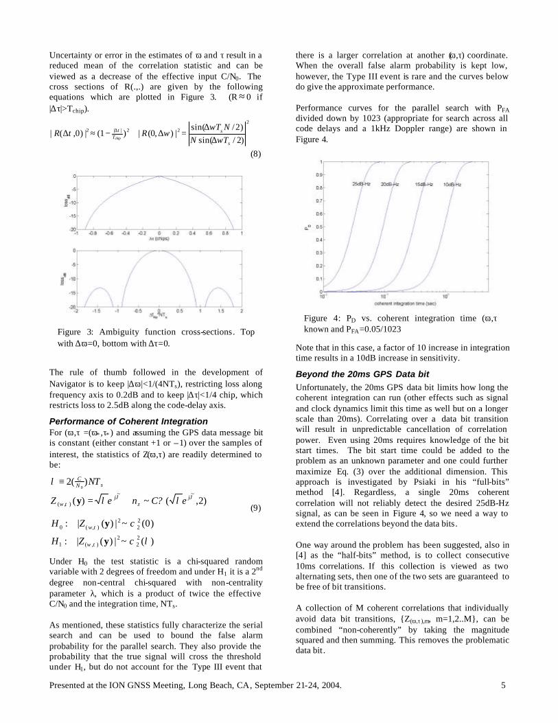
there is a larger correlation at another (ω,τ) coordinate. When the overall false alarm probability is kept low, however, the Type III event is rare and the curves below do give the approximate performance. Performance curves for the parallel search with PFA divided down by 1023 (appropriate for search across all code delays and a 1kHz Doppler range) are shown in Figure 4.

Figure 4: PD vs. coherent integration time (ω,τ) known and PFA=0.05/1023

Note that in this case, a factor of 10 increase in integration time results in a 10dB increase in sensitivity.

Beyond the 20ms GPS Data bit Unfortunately, the 20ms GPS data bit limits how long the coherent integration can run (other effects such as signal and clock dynamics limit this time as well but on a longer scale than 20ms). Correlating over a data bit transition will result in unpredictable cancellation of correlation power. Even using 20ms requires knowledge of the bit start times. The bit start time could be added to the problem as an unknown parameter and one could further maximize Eq. (3) over the additional dimension. This approach is investigated by Psiaki in his “full-bits” method [4]. Regardless, a single 20ms coherent correlation will not reliably detect the desired 25dB-Hz signal, as can be seen in Figure 4, so we need a way to extend the correlations beyond the data bits. One way around the problem has been suggested, also in [4] as the “half-bits” method, is to collect consecutive 10ms correlations. If this collection is viewed as two alternating sets, then one of the two sets are guaranteed to be free of bit transitions. A collection of M coherent correlations that individually avoid data bit transitions, {Z(ω,τ ),m, m=1,2..M}, can be combined “non-coherently” by taking the magnitude squared and then summing. This removes the problematic data bit.


),(),(*

1

0

2),,(),(

max

||

τωτω

τωτω

QQ

ZQM

mm

=

= ∑−

= (10)

Q* is then used as the test statistic to be compared against a threshold. This is the “Plong” detection statistic Psiaki suggests in [4] and justifies as the Locally Most Powerful (LMP) test under his assumptions. This type of combined coherent/non-coherent integration was previously suggested for GPS signal acquisition by [10] and has been commonly used since. Throughout the rest of the paper, this method of non-coherently combining M coherent integrations of duration L ms (i.e. N=(L*0.001)/Ts samples) each will be referred to as the “L/M integration.” Another important reason to keep the coherent integration period short is because of the structure of the ambiguity function along the frequency axis, as discussed above. Correlations can be combined non-coherently for as long as desired without the need for increasing frequency resolution. For 10ms coherent integration, a 25Hz grid spacing will result in a worst case loss of only 0.2dB.

Performance of Non-coherent Integration

Again, for (ω,τ) =(ω∗ ,τ∗ ) and assuming data-bit transitions have been avoided in each coherent integration interval, the statistics of Q are readily determined to be:

)(~)(:

)0(~)(:22),(1

22),(0

λχ

χ

τω

τω

MQH

QH

M

M

y

y (11)

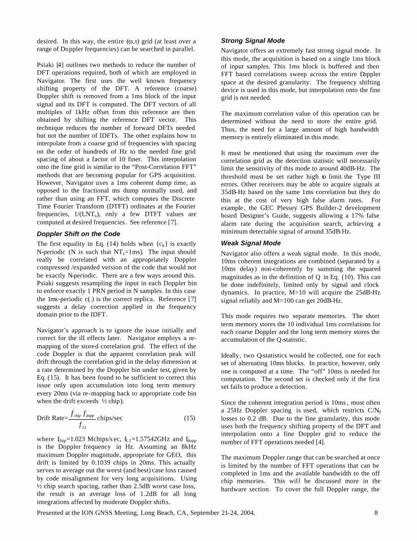
Performance curves for the parallel search with PFA divided down by 1023 are shown in Figure 5.

Figure 5: PD vs. total integration time for 10/M integrations with (ω,τ) known and PFA=0.05/1023

As may be expected, the gains from non-coherent integration come more slowly than from coherent integration. Sensitivity increases roughly with the square

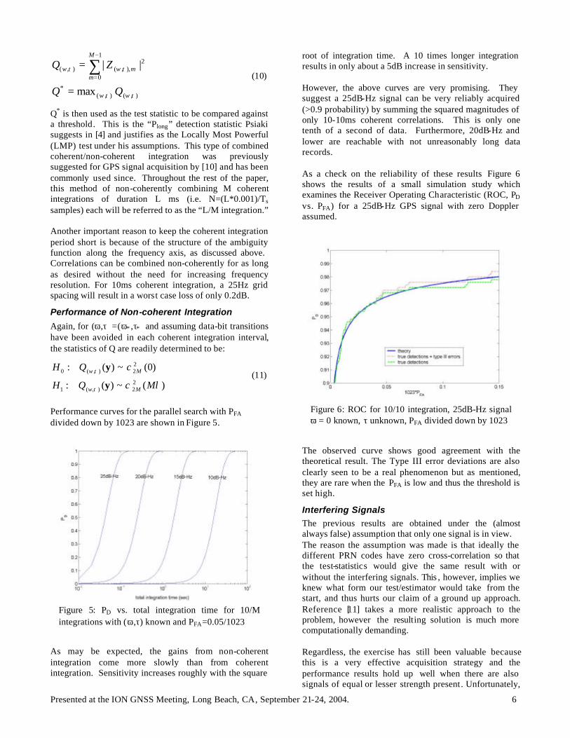
root of integration time. A 10 times longer integration results in only about a 5dB increase in sensitivity. However, the above curves are very promising. They suggest a 25dB-Hz signal can be very reliably acquired (>0.9 probability) by summing the squared magnitudes of only 10-10ms coherent correlations. This is only one tenth of a second of data. Furthermore, 20dB-Hz and lower are reachable with not unreasonably long data records. As a check on the reliability of these results Figure 6 shows the results of a small simulation study which examines the Receiver Operating Characteristic (ROC, PD vs. PFA) for a 25dB-Hz GPS signal with zero Doppler assumed.

Figure 6: ROC for 10/10 integration, 25dB-Hz signal ω = 0 known, τ unknown, PFA divided down by 1023

The observed curve shows good agreement with the theoretical result. The Type III error deviations are also clearly seen to be a real phenomenon but as mentioned, they are rare when the PFA is low and thus the threshold is set high.

Interfering Signals The previous results are obtained under the (almost always false) assumption that only one signal is in view. The reason the assumption was made is that ideally the different PRN codes have zero cross-correlation so that the test-statistics would give the same result with or without the interfering signals. This , however, implies we knew what form our test/estimator would take from the start, and thus hurts our claim of a ground up approach. Reference [11] takes a more realistic approach to the problem, however the resulting solution is much more computationally demanding. Regardless, the exercise has still been valuable because this is a very effective acquisition strategy and the performance results hold up well when there are also signals of equal or lesser strength present. Unfortunately,


the performance results do not hold up when many strong signals are present as well. This is due to the non-ideal cross-correlation properties of the C/A codes . The cross-correlation rejection for the C/A code is known to be about 23dB [9]. The primary effect of interfering signals is that the cross-correlation peaks cause the number of false alarms to increase for a given threshold level. The simplest solution is to increase the thresholds to control the PFA and correspondingly increase the integration intervals to recover PD. This will work when the power difference is moderate, but will fail for very large disparities (>15-20dB), at which point the acquisition of the weak signal becomes hopeless without somehow dealing with the interfering signal. One possible solution is through careful selection among the available antennas on the spacecraft or through the use of antenna phasing to help reject the unwanted strong “jamming” signal. Alternatively, one can try to acquire and track the strong signals first and then cancel them out of the input before attempting the weak signals. This is suggested by [9], demonstrated with success by Psiaki [4] and is what is effectively done in the ML GPS Receiver of [11]. During tracking, precise estimates of (ω,τ,θ) are maintained and all that is additionally needed is the signal amplitude, |A|, whose ML estimate was given in Eq. (4). It is possible to use this in online processing and it may be incorporated in the Navigator design in the future.

NAVIGATOR RECEIVER ALGORITHMS The Navigator receiver can quickly and reliably acquire and track signals down to 25dB-Hz and lower by employing special hardware that computes the Q*-statistic described above.

Navigator Design Principles The Navigator receiver design is based upon two central design principles. First, Navigator is intended to operate totally autonomously. That is, it does not require external data aiding or any other a priori information such as a current estimate of time, a recent GPS almanac or a converged navigation filter estimate of the receiver dynamics, etc. If such a priori information was available then Navigator may be able to make use of it, but it is not assumed. Second, Navigator operates in real time. Data is double buffered up front in 1ms blocks and processed as it comes in. Some advocate the use of large up front storage to buffer the entire record of sampled data needed for acquisition. Processing can then occur with relaxed time constraints, only needing to be so fast that the (ω,τ) estimate will still be valid when processing finishes. Then the receiver could operate in a faster than real-time mode to catch up with the streaming input, or simply begin tracking on the most recent samples. The problem with this method is that it requires a large up-front

memory that can be very expensive for a space qualified part. Further, the performance is ultimately limited by the size of this memory.

DFT-Based calculation of the correlation statistic The primary computational device employed by Navigator is the use of the DFT to calculate the 1ms correlations. When the FFT algorithm is used to compute these DFTs, large computational savings are achieved. Specifically, when an N-point DFT is computed using the FFT, the savings are of order N/log2(N) over direct computation. This method calculates all code delay correlations in ½ chip increments (for our implementation) using a single 1ms block of data. This is a well known technique used for GPS and more generally for Direct Sequence Spread Spectrum (DSSS) signal acquisition. See [12] and its associated references. Let x=(x0, x1 …xN-1)’ be a signal and X=(X0, X1…XN-1) be its DFT sequence (likewise for c and C). The “circular-correlation property” gives the following identity (where o means point by point multiplication of the vectors):

nNnk

N

kkn IDFTcxZ ][ *

mod)(

1

0

CX o== +

−

=∑ (12)

To apply this to our problem, use a 1ms block of the baseband downconverted input signal (in parentheses below) as the x and the DFT of the code sequence as C, which can be computed offline, and compute (let τ now represent an integer offset of the code between 0 and N-1):

ττω

τω

τω

][)(

)()(

*mod)(

1

0

1

0),(

CX

y

oIDFTcey

ceyZ

Nk

N

k

kTjk

k

N

k

kTjk

s

s

==

=

+

−

=

−

+

−

=

−

∑

∑ (13)

This gives the 1ms correlation. The effect of Doppler shift on the code sequence is ignored for now and will be discussed below. To get a longer correlation, add L consecutive 1ms block correlations:

∑∑ ∑

∑−

=

−

=+

−+

=

−

−

=

−+

==

=

1

0

*1

0mod)(

1)1(

1

0),(

][)(

)(

L

ll

L

lNk

lN

Nlk

kTjk

LN

k

kTjkk

IDFTcey

ecyZ

s

s

ττω

ωττω

CX

y

o

(14)

Just repeat this calculation and add up the squared magnitudes to get the desired Q-statistic. The Navigator acquisition hardware implements exactly this process. With this method, the Q-statistic is calculated for the entire code dimension based on a single block of input data. Further, if many FFTs can be completed in 1ms then the search across the Doppler dimension can be done as well. To do so, just repeat this method for each frequency on the search grid at whatever frequency granularity


desired. In this way, the entire (ω,τ) grid (at least over a range of Doppler frequencies) can be searched in parallel. Psiaki [4] outlines two methods to reduce the number of DFT operations required, both of which are employed in Navigator. The first uses the well known frequency shifting property of the DFT. A reference (coarse) Doppler shift is removed from a 1ms block of the input signal and its DFT is computed. The DFT vectors of all multiples of 1kHz offset from this reference are then obtained by shifting the reference DFT vector. This technique reduces the number of forward DFTs needed but not the number of IDFTs. The other explains how to interpolate from a coarse grid of frequencies with spacing on the order of hundreds of Hz to the needed fine grid spacing of about a factor of 10 finer. This interpolation onto the fine grid is similar to the “Post-Correlation FFT” methods that are becoming popular for GPS acquisition. However, Navigator uses a 1ms coherent dump time, as opposed to the fractional ms dump normally used, and rather than using an FFT, which computes the Discrete Time Fourier Transform (DTFT) ordinates at the Fourier frequencies, 1/(LNTs), only a few DTFT values are computed at desired frequencies. See reference [7].

Doppler Shift on the Code The first equality in Eq. (14) holds when {ck} is exactly N-periodic (N is such that NTs=1ms). The input should really be correlated with an appropriately Doppler compressed /expanded version of the code that would not be exactly N-periodic. There are a few ways around this. Psiaki suggests resampling the input in each Doppler bin to enforce exactly 1 PRN period in N samples. In this case the 1ms-periodic c(.) is the correct replica. Reference [7] suggests a delay correction applied in the frequency domain prior to the IDFT. Navigator’s approach is to ignore the issue initially and correct for the ill effects later. Navigator employs a re-mapping of the stored correlation grid. The effect of the code Doppler is that the apparent correlation peak will drift through the correlation grid in the delay dimension at a rate determined by the Doppler bin under test, given by Eq. (15). It has been found to be sufficient to correct this issue only upon accumulation into long term memory every 20ms (via re-mapping back to appropriate code bin when the drift exceeds ½ chip).

Drift Rate=1L

doppchip

f

ffchips/sec (15)

where fchip=1.023 Mchips/s ec, fL1=1.57542GHz and fdopp is the Doppler frequency in Hz. Assuming an 8kHz maximum Doppler magnitude, appropriate for GEO, this drift is limited by 0.1039 chips in 20ms. This actually serves to average out the worst (and best) case loss caused by code misalignment for very long acquisitions. Using ½ chip search spacing, rather than 2.5dB worst case loss, the result is an average loss of 1.2dB for all long integrations affected by moderate Doppler shifts.

Strong Signal Mode Navigator offers an extremely fast strong signal mode. In this mode, the acquisition is based on a single 1ms block of input samples. This 1ms block is buffered and then FFT based correlations sweep across the entire Doppler space at the desired granularity. The frequency shifting device is used in this mode, but interpolation onto the fine grid is not needed. The maximum correlation value of this operation can be determined without the need to store the entire grid. Thus, the need for a large amount of high bandwidth memory is entirely eliminated in this mode. It must be mentioned that using the maximum over the correlation grid as the detection statistic will necessarily limit the sensitivity of this mode to around 40dB-Hz. The threshold must be set rather high to limit the Type III errors. Other receivers may be able to acquire signals at 35dB-Hz based on the same 1ms correlation but they do this at the cost of very high false alarm rates. For example , the GEC Plessey GPS Builder-2 development board Designer’s Guide, suggests allowing a 17% false alarm rate during the acquisition search, achieving a minimum detectable signal of around 35dB-Hz.

Weak Signal Mode

Navigator also offers a weak signal mode. In this mode, 10ms coherent integrations are combined (separated by a 10ms delay) non-coherently by summing the squared magnitudes as in the definition of Q in Eq. (10). This can be done indefinitely, limited only by signal and clock dynamics. In practice, M=10 will acquire the 25dB-Hz signal reliably and M=100 can get 20dB-Hz. This mode requires two separate memories. The short term memory stores the 10 individual 1ms correlations for each coarse Doppler and the long term memory stores the accumulation of the Q-statistic. Ideally, two Q-statistics would be collected, one for each set of alternating 10ms blocks. In practice, however, only one is computed at a time. The “off” 10ms is needed for computation. The second set is checked only if the first set fails to produce a detection. Since the coherent integration period is 10ms , most often a 25Hz Doppler spacing is used, which restricts C/N0 losses to 0.2 dB. Due to the fine granularity, this mode uses both the frequency shifting property of the DFT and interpolation onto a fine Doppler grid to reduce the number of FFT operations needed [4]. The maximum Doppler range that can be searched at once is limited by the number of FFT operations that can be completed in 1ms and the available bandwidth to the off chip memories. This will be discussed more in the hardware section. To cover the full Doppler range, the


frequencies are searched sequentially in this maximum Doppler block size. Arbitrary L/M modes are available as well, but Navigator most commonly uses 1/1 (strong) and 10/M (weak). For example, if data-aiding is available then L>10 may be desirable.

Fine Acquisition

In weak signal mode, the (ω,τ) estimate provided by the acquisition module may not be accurate enough to initialize tracking, particularly in the ω dimension. Furthermore, determination of the location of the GPS data bit transition is essential when tracking weak signals. When the acquisition terminates with a successful detection, the estimated (ω,τ) is used to initialize a tracking correlator/channel. Open loop 1-PRN (~1ms) period accumulations are collected for a specified amount of time, e.g. J-PRN periods, during which the following statistic is calculated to determine an estimate of the bit transition time, i.e. to get bit lock (K=floor(J/20)).

∑ ∑−

=

++

+=∈=

1

0

21920

20}19,..0{

* maxargK

k

lk

lkj jl

Zl (16)

This assumes that the initial frequency estimate is good enough so residual frequency error does not wash out the above 20ms correlations. Following the aforementioned rule of thumb implies assuring |∆ω|<12.5Hz before attempting to compute Eq. (16). To resolve frequency more finely, we can process the same type of {Zk} post-correlation sequence. When the replica phase is kept continuous over K consecutive L ms coherent integration blocks, the individual correlations have the form:

kLNTkj

kk nebdZ s += ∆ )(ω (17)

Here, dk is the GPS data bit and b is a complex constant (essentially) independent of k. This being so, if we square each Zk (to remove the data bit), then we get a pure complex exponential plus (non-Gaussian) noise, for which, the maximum of the periodogram is an often used estimator of frequency. We can use the FFT engine to compute the periodogram and maximize it to get an estimate of 2∆ω. This has been shown to work nicely in the lab, using L = 1ms, for signals even below 25dB-Hz with J = 2048, giving a resolution of <1Hz for ∆ω. For smaller J, we zero-pad the Z-squared sequence. This assumes the frequency rate is small enough so the residual Doppler is roughly constant over J*L-ms. Depending on the situation, the two calculations can be done simultaneously, or first (16) then (17), or vice-versa.

Tracking

Navigator employs standard FLL/PLL/DLL tracking methods using 1ms correlations for strong signals and

with correlations extended to 20ms for tracking weak signals. It is shown in reference [10] that PLL phase tracking to 25dB-Hz is achievable with 20ms correlations and a good oscillator. Carrier phase tracking is known to be the weak link as compared with carrier frequency and code tracking. The theoretical bit error probability at C/N0=25dB-Hz is ~10-4 for (perfect) coherent demodulation of BPSK signals, so data demodulation can be done relatively well. Much below 25dB-Hz, using traditional FLL/PLL/DLL tracking, reliable data demodulation becomes difficult and phase tracking begins to fail. Bit error probabilities can be improved by averaging many cycles of the repeating GPS data message. This method may be employed in Navigator in the future. In [5], Psiaki demonstrates reliable zero a priori signal tracking and data demodulation of the C/A signal down to 15dB-Hz using extended Kalman filter methods. These methods have been thoroughly investigated by the authors, but were deemed to be too computationally intensive for the first implementation of Navigator.

NAVIGATOR HARDWARE DESIGN The Navigator receiver employs the conventional GPS receiver design consisting of a bank of hardware correlators controlled by a general purpose microprocessor. In addition, it adds a specialized acquisition module that rapidly calculates the long term detection statistic, Q*. A block diagram of the top-level Navigator design is shown in Figure 9.

MicroprocessorAnalog

Front End

Antenna

TrackingCorrelators

Acquisition Module

Memory

MicroprocessorAnalog

Front End

Antenna

TrackingCorrelators

Acquisition Module

Memory

Figure 9: System Block Diagram

All of the GPS specific hardware is implemented in VHDL to target rad-hard FPGAs. The reason for targeting FPGAs rather than an ASIC is partially cost constraint, but more importantly to maintain flexibility. Navigator is expected to grow in the near future (e.g. L2C functionality is to be added) and will act as a stepping stone for future GPS receiver development. FPGA implementation offers the greatest flexibility for growth and modification of the design. This is particularly important for space applications because it means that Navigator can be customized to best fit mission specific goals and requirements.


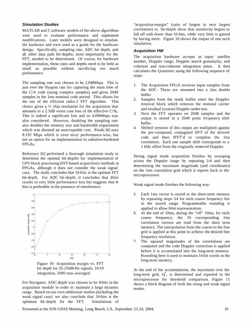
Simulation Studies MATLAB and C software models of the above algorithms were used to evaluate performance and implement modifications. Later models were designed to emulate the hardware and were used as a guide for the hardware design. Specifically, sampling rate, ADC bit depth, and all other data path bit-depths, most importantly for the FFT, needed to be determined. Of course, for hardware implementation, these rates and depths need to be held as small as possible without sacrificing too much performance. The sampling rate was chosen to be 2.048Msps. This is just over the Nyquist rate for capturing the main lobe of the C/A code (using complex samples) and gives 2048 samples in the 1ms nominal code period. This allows for the use of the efficient radix-2 FFT algorithm. This choice gives a ½ chip resolution for the acquisition that amounts to a 2.5dB worst case loss of the effective C/N0. This is indeed a significant loss and so 4.096Msps was also considered. However, doubling the sampling rate also doubles the memory size and bandwidth requirement which was deemed an unacceptable cost. Psiaki [4] uses 8.192 Msps which is even nicer performance-wise, but not an option for an implementation in radiation-hardened FPGAs. Reference [6] performed a thorough simulation study to determine the optimal bit-depths for implementation of GPS block processing (FFT-based acquisition) methods in FPGAs, although it does not consider the weak signal case. The study concludes that 10-bits is the optimal FFT bit-depth. For ADC bit-depth, it concludes that 2-bits results in very little performance loss but suggests that 8-bits is preferable in the presence of interference.

Figure 10: Acquisition margin vs. FFT bit depth for 25-29dB-Hz signals, 10/10 integration, 2000 runs averaged.

For Navigator, ADC depth was chosen to be 8-bits in the acquisition module in order to maintain a large dynamic range. Based on our own additional studies (including the weak signal case) we also conclude that 10-bits is the optimum bit -depth for the FFT. Simulations of

“acquisition-margin” (ratio of largest to next largest correlation) vs. bit-depth show that sensitivity begins to fall off with fewer than 10-bits, while very little is gained by having more. Figure 10 shows the output of one such simulation.

Acquisition HW The acquisition hardware accepts as input: satellite number, Doppler range, Doppler search granularity, and coherent and non-coherent integration times. It then calculates the Q-statistic using the following sequence of steps. 1. The Acquisition FPGA receives input samples from

the ADC. These are streamed into a 2ms double buffer.

2. Samples from the ready buffer enter the Doppler removal block which removes the nominal carrier and residual (coarse) Doppler under test.

3. Next the FFT operates on 2048 samples and the output is stored in a 2048 point frequency shift buffer.

4. Shifted versions of this output are multiplied against the pre-computed, conjugated DFT of the desired code and then IFFT’d to complete the 1ms correlation. Each one sample shift corresponds to a 1 kHz offset from the originally removed Doppler.

Strong signal mode acquisition finishes by sweeping across the Doppler range by repeating 2-4 and then determining the maximum magnitude (and coordinates) on the 1ms correlation grid which it reports back to the microprocessor. Weak signal mode finishes the following way: 5. Each 1ms vector is stored to the short-term memory

by repeating steps 3-4 for each coarse frequency bin in the search range. Programmable rounding is applied to allow 8-bit representation.

6. At the end of 10ms, during the “off” 10ms, for each coarse frequency, the 10 corresponding 1ms correlation vectors are read from the short term memory. The interpolation from the coarse to the fine grid is applied at this point to achieve the desired fine frequency resolution.

7. The squared magnitudes of the correlations are computed and the code Doppler correction is applied before it is accumulated into the long-term memory. Rounding here is used to maintain 16-bit words in the long-term memory.

At the end of the accumulations, the maximum over the long-term grid, Q*, is determined and reported to the microprocessor for threshold comparison. Figure 11 shows a block diagram of both the stong and weak signal modes.


pre-computed FFT’d

PRN codes

1ms

|.|2

FFT

X

1ms coherent correlation

memory

IFFT

1ms

peak correlation

detector

+

Analog Front End

1ms freq shift buffer

residualDopplerremoval

code Doppler correct

Micro-processor(ColdFire)

long- term correlation

memory

10ms coherent

combination (DFT)

1ms

|.|2

Weak Signal Mode Only

“Frequency Domain” Correlation

pre-computed FFT’d

PRN codes

1ms

|.|2

FFT

X

1ms coherent correlation

memory

IFFT

1ms

peak correlation

detector

+

Analog Front End

1ms freq shift buffer

residualDopplerremoval

code Doppler correct

Micro-processor(ColdFire)

long- term correlation

memory

10ms coherent

combination (DFT)

1ms

|.|2

Weak Signal Mode Only

“Frequency Domain” Correlation

Figure 11: Dual mode acquisition block diagram

Two potential bottlenecks limit the performance of the acquisition module: the bandwidth to off-chip SRAM (for accumulation of the correlation grids) and speed of the FFT operation, which is ultimately determined by the size of the FPGA. Running this algorithm in real-time requires a huge bandwidth to the off chip SRAM. To provide for this bandwidth, a 64-bit bus connects the SRAM to the acquisition FPGA. Running at 66MHz, this provides a 528MB/s bandwidth. Weak signal mode requires 32.8MB/s bandwidth per 1kHz Doppler search block and thus can cover 16kHz at once if limited only by memory bandwidth. The second bottleneck is in running the FFTs fast enough. The hardware has the capability of performing 23FFTs/ms . Assuming a 250Hz coarse Doppler spacing, this implies a maximum one pass Doppler coverage of 5.5kHz. The current design uses 4 parallel butterfly adders to implement the FFT, limited by the expected utilization of the flight FPGA. If the usage estimates are proven to be too conservative, the number of butterfly adders could be increased, providing improved FFT speed.

Tracking Hardware

The tracking FPGA consists of a standard block of hardware correlators. However, to improve FPGA usage efficiency, rather than processing samples at the sampling rate, data are stored in a FIFO and processed by time shared hardware running at a much higher rate than the sampler. The specific implementation consists of 3 time shared correlator blocks that give 12 channels each, for a total of 36 channels.

Receiver Flight Part Selection

Navigator has been designed to provide the highest levels of reliability in the severe radiation environment present in high Earth orbits: 1. All parts must be able to withstand a Total Dose

radiation level of 100 krad. This exposure is with no box shielding; spot shielding is permissible.

2. All parts must be tolerant to a 37 MeV-cm2/mg exposure, with no SEUs (single event upsets).

3. All parts must be SEL (single event latch-up) immune up to 90 MeV-cm2/mg.

Selecting parts that provide the required performance and survivability is a significant design challenge. The flight RF front end will be built around Peregrine Semiconductor’s PE8510x L1/L2 GPS front end ASIC. For the FPGAs, the Actel RTAX-2000 was selected. This is the largest rad-hard part offered by Actel as of the writing of this paper. The combinatorial and sequential logic meet Navigator’s radiation requirements. The RAMs on the Actel FPGA are actually considered soft (not immune from SEUs); however, Actel offers different EDAC (Error Detection and Correction) algorithms in their tool set to increase the data resiliency of SRAM. The flight SRAM will be a 4 BAE SRAM die packaged in MCM (Multi-Chip Module) by 3D-Plus. The baseline flight oscillator will be an ovenized crystal oscillator (OXO); however, a version of the receiver will be available using a high quality temperature controlled crystal oscillator (TCXO) for applications that wish to trade some power, mass, and cost savings for slightly reduced performance. The RH-CF5208 ColdFire was chosen as the primary microprocessor. It is a true embedded processor with very low-power consumption and almost no glue logic. The primary disadvantage of the ColdFire is its relatively modest computational power (~60 MIPS @ 66MHz) and lack of a floating-point unit. This has been partially compensated for by a custom implementation of a floating point co-processor in the FPGAs. The Navigator project has been able to take advantage of the ongoing development of the Subsystem Data Node (SDN), for NASA’s Solar Dynamics Observatory (SDO) which provides the ColdFire CPU and external interfaces integrated on a 6U-220 Compact PCI card, shown in Figure 12. The Core SDN design places the RH-CF5208 CPU and peripherals (including MIL-STD-1553, RS-422, cPCI, EEPROM, and an ADC) on half of a 6U-220 Compact PCI card. The other half is reserved for application specific hardware, in this case the GPS receiver hardware.


Figure 12: Core SDN, right half will host the GPS specific hardware in the Navigator flight design.

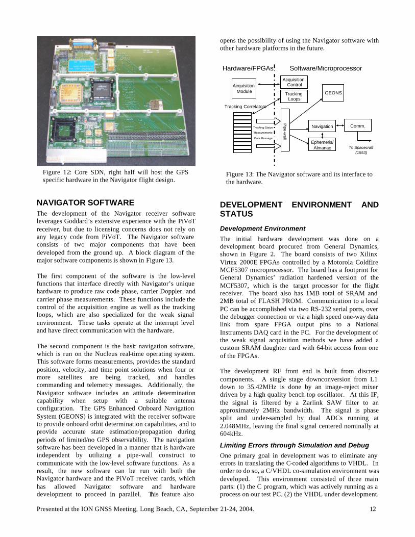
NAVIGATOR SOFTWARE The development of the Navigator receiver software leverages Goddard’s extensive experience with the PiVoT receiver, but due to licensing concerns does not rely on any legacy code from PiVoT. The Navigator software consists of two major components that have been developed from the ground up. A block diagram of the major software components is shown in Figure 13. The first component of the software is the low-level functions that interface directly with Navigator’s unique hardware to produce raw code phase, carrier Doppler, and carrier phase measurements. These functions include the control of the acquisition engine as well as the tracking loops, which are also specialized for the weak signal environment. These tasks operate at the interrupt level and have direct communication with the hardware. The second component is the basic navigation software, which is run on the Nucleus real-time operating system. This software forms measurements, provides the standard position, velocity, and time point solutions when four or more satellites are being tracked, and handles commanding and telemetry messages. Additionally, the Navigator software includes an attitude determination capability when setup with a suitable antenna configuration. The GPS Enhanced Onboard Navigation System (GEONS) is integrated with the receiver software to provide onboard orbit determination capabilities, and to provide accurate state estimation/propagation during periods of limited/no GPS observability. The navigation software has been developed in a manner that is hardware independent by utilizing a pipe-wall construct to communicate with the low-level software functions. As a result, the new software can be run with both the Navigator hardware and the PiVoT receiver cards, which has allowed Navigator software and hardware development to proceed in parallel. This feature also

opens the possibility of using the Navigator software with other hardware platforms in the future.

Pipe

-wall

Hardware/FPGAs

Acquisition Module Tracking

Loops

Acquisition Control

GEONS

Navigation

Ephemeris/Almanac

Comm.

Software/Microprocessor

Tracking Status

Measurements

Data Message

Tracking Correlators

To Spacecraft(1553)

Figure 13: The Navigator software and its interface to the hardware.

DEVELOPMENT ENVIRONMENT AND STATUS

Development Environment

The initial hardware development was done on a development board procured from General Dynamics, shown in Figure 2. The board consists of two Xilinx Virtex 2000E FPGAs controlled by a Motorola Coldfire MCF5307 microprocessor. The board has a footprint for General Dynamics’ radiation hardened version of the MCF5307, which is the target processor for the flight receiver. The board also has 1MB total of SRAM and 2MB total of FLASH PROM. Communication to a local PC can be accomplished via two RS-232 serial ports, over the debugger connection or via a high speed one-way data link from spare FPGA output pins to a National Instruments DAQ card in the PC. For the development of the weak signal acquisition methods we have added a custom SRAM daughter card with 64-bit access from one of the FPGAs. The development RF front end is built from discrete components. A single stage downconversion from L1 down to 35.42MHz is done by an image-reject mixer driven by a high quality bench top oscillator. At this IF, the signal is filtered by a Zarlink SAW filter to an approximately 2MHz bandwidth. The signal is phase split and under-sampled by dual ADCs running at 2.048MHz, leaving the final signal centered nominally at 604kHz.

Limiting Errors through Simulation and Debug

One primary goal in development was to eliminate any errors in translating the C-coded algorithms to VHDL. In order to do so, a C/VHDL co-simulation environment was developed. This environment consisted of three main parts: (1) the C program, which was actively running as a process on our test PC, (2) the VHDL under development,


which was running in simulation as a second process on the PC, and (3) a gasket (implemented as a software pipe) to allow the two processes to talk to one another. A common data file was fed into both the C and the VHDL processes. Through the gasket the results of the tracking and acquisition were compared every millisecond and any discrepancies were immediately flagged. Each simulation generated a log file describing its behavior any particular data transfers, any interrupts and, any errors. Each logic element in the acquisition FPGA contains an upstream and downstream debug RAM block. These RAMs are used to determine the proper execution of the algorithm. Any element (beginning with the Doppler Removal Block and ending with the IFFT) can be tested to ensure that it is behaving properly.

Status Development of the Navigator receiver is continuing using the commercial ColdFire and Xilinx FPGAs implemented on the development board shown in Figure 2. The receiver is being tested using GPS signals from multiple sources: a basic GPS signal generator capable of generating a single GPS channel and dynamics, a Spirent STR4500 GPS simulator, and live GPS signals from a rooftop antenna. Fast signal acquisition and tracking has been successfully demonstrated on strong signals (C/N0>40dB-Hz) with LEO dynamics. For a Doppler uncertainty range of ±50kHz and using a frequency search granularity of 250Hz, the receiver acquires satellites on 12 channels in less than 2 seconds with zero a priori knowledge. Weak signal acquisition has been shown to acquire 25dB-Hz signals reliably using the 10/10 integration. Considerably weaker signals have also been acquired using longer integrations. In weak signal mode, the Doppler range that can be covered in one pass is currently 5.7kHz at 25Hz granularity. For development, Navigator will offer 36 tracking channels and utilize 60% of one Xilinx FPGA , while acquisition will use approximately 75% of a second FPGA. The rad-hard Actel FPGAs offers less logic and RAM then the Xilinx counterparts, and thus will have higher utilization rates. For the flight design, acquisition will use two Actel FPGAs each at 40% utilization, while tracking will use 70% of a third FPGA. As the sum of the utilizations of the two flight acquisition FPGAs do not total 100%, it is possible that the acquisition design may fit in a single FPGA. However, the design still plans for three Actels total, which allows room for growth or features. For example, a floating point coprocessor has been implemented in the FPGAs to assist the ColdFire in its computational tasks. The “breadboard” version of the Navigator hardware will employ most of the flight parts. In particular, Actels (commercial AX2000’s, not the rad-hard version) rather

than Xilinx, the rad-hard ColdFire and SRAM, the RF front end and the OXO. Currently, the schematic capture for the breadboard design is underway. The breadboard version is expected to be ready in mid 2005.

SUMMARY Navigator is being developed as a fully space flight qualified GPS receiver optimized for fast signal acquisition and weak signal tracking. Considerable effort has been put forth to implement what is generally considered a non-real time software GPS receiver algorithm into real time hardware. The fast acquisition capabilities provide exceptional TTFF performance with no a priori receiver state or GPS almanac information, even in the presence of high Doppler shifts associated with LEO (or near perigee in highly eccentric orbits). The fast acquisition capability also makes it feasible to implement extended correlation intervals and therefore significantly reduce Navigator’s acquisition threshold. Fast acquisition and weak signal tracking algorithms have been implemented and validated on a hardware development board. The ultimate goal is to license the Navigator design to an industry partner who will then market the receiver as a commercial product. A fully functional “breadboard” version of the receiver with integrated navigation software is expected by mid 2005.

REFERENCES 1. J. R. Carpenter, D. C. Folta, M. C. Moreau, and D. A.

Quinn. “Libration point navigation concepts supporting the vision for space exploration.” To appear in Astrodynamics 2004. Univelt, 2004.

2. Kronman, J.D., "Experience Using GPS For Orbit Determination of a Geosynchronous Satellite," Proceedings of the Institute of Navigation GPS 2000 Conference, Salt Lake City, UT, September 2000.

3. C. Mehlen, D. Laurichesse, "Real-Time GEO Orbit Determination Using TOPSTAR 3000 GPS Receiver," Navigation , Vol. 48, No. 3, Fall 2001, pp. 169-180.

4. Psiaki, M. L. “Block Acquisition of Weak GPS Signals in a Software Receiver,” Proceedings of the Institute of Navigation GPS 2001 Conference, Salt Lake City, Utah, September 2001, pp.2838-2850.

5. Psiaki, M. L. “Extended Kalman Filter Methods for Tracking Weak GPS signals,” Proceedings of the Institute of Navigation GPS 2002 Conference, September 2002, pp.2539-2553

6. Gunawardena, S., “Feasibility Study for the Implementation of Global Positioning System Block Processing Techniques in Field Programmable Gate Arrays,” Masters Thesis. Ohio University, Nov. 2000.

7. Akopian, David, “A Fast Satellite Acquisition Method”, Proceedings of the Institute of Navigation GPS 2001 Conference, Salt Lake City, Utah, September 2001. pp. 2871-2881


8. Kay, Stephen, “Fundamentals of Statistical Signal Processing, Vol 2: Detection Theory, Ch. 7,” Prentice Hall PTR. Upper Saddle River, NJ. 1998.

9. Spilker, J.J., “Signal Structure and Theoretical Performance,” in Global Positioning System:Theory and Applications, Vol 1., B.W.Parkinson and J.J. Spilker Jr., Eds. Washington, DC: American institute of Aeronautics and Astronautics, 1996, ch. 3, pp.57-119.

10. Van Dierondonck, A.J., “GPS Receivers,” in Global Positioning System:Theory and Applications, Vol 1., B.W.Parkinson and J.J. Spilker Jr., Eds. Washington, DC: American institute of Aeronautics and Astronautics, 1996, ch. 8, pp.329-407.

11. Progri, I.F., Bromberg, M.C., Michalson W.R., “The Acquisition Process of a Maximum Likelihood GPS Receiver,” Proceedings of the Institute of Navigation GPS/GNSS 2003 Conference, September 2003, pp.2532-2542.

12. Tsui, J.B.Y. “Fundamentals of Global Positioning System Receivers: A Software Approach,” John Wiley &Sons Inc, 2000.

Navigator GPS Receiver for Fast Acquisition and Weak Signal Space Applications

Documents

Transcript of Navigator GPS Receiver for Fast Acquisition and Weak Signal Space Applications