Navigating the multiple meanings of diversity: a roadmap ...

I D E A A N DP E R S P E C T I V E Navigating the multiple meanings of b diversity:

a roadmap for the practicing ecologist

Marti J. Anderson,1* Thomas O.

Crist,2 Jonathan M. Chase,3 Mark

Vellend,4 Brian D. Inouye,5 Amy L.

Freestone,6 Nathan J. Sanders,7

Howard V. Cornell,8 Liza S.

Comita,9 Kendi F. Davies,10 Susan

P. Harrison,8 Nathan J. B. Kraft,11

James C. Stegen12 and Nathan G.

Swenson13

Abstract

A recent increase in studies of b diversity has yielded a confusing array of concepts,

measures and methods. Here, we provide a roadmap of the most widely used and

ecologically relevant approaches for analysis through a series of mission statements.

We distinguish two types of b diversity: directional turnover along a gradient vs. non-

directional variation. Different measures emphasize different properties of ecological

data. Such properties include the degree of emphasis on presence ⁄ absence vs. relative

abundance information and the inclusion vs. exclusion of joint absences. Judicious use of

multiple measures in concert can uncover the underlying nature of patterns in b diversity

for a given dataset. A case study of Indonesian coral assemblages shows the utility of a

multi-faceted approach. We advocate careful consideration of relevant questions,

matched by appropriate analyses. The rigorous application of null models will also help

to reveal potential processes driving observed patterns in b diversity.

Keywords

Biodiversity, community ecology, environmental gradients, heterogeneity, multivariate

analysis, species composition, turnover, variance partitioning, variation.

Ecology Letters (2010)

I N T R O D U C T I O N

b diversity, generally defined as variation in the identities of

species among sites, provides a direct link between

biodiversity at local scales (a diversity) and the broader

regional species pool (c diversity) (Whittaker 1960, 1972).

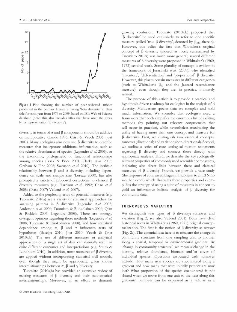
The past decade has witnessed an especially marked increase

in studies under the name of b diversity (Fig. 1). Indeed, the

study of b diversity is genuinely at the heart of community

ecology – what makes assemblages of species more or less

similar to one another at different places and times (Vellend

2010)?

Many different measures of b diversity have been

introduced, but there is no overall consensus about which

ones are most appropriate for addressing particular ecolog-

ical questions (Vellend 2001; Koleff et al. 2003; Jost 2007;

Jurasinski et al. 2009; Tuomisto 2010a,b). Debates persist

regarding whether the measures used for partitioning c

1Institute of Information and Mathematical Sciences (IIMS),

Massey University, Albany Campus, Auckland, New Zealand2Department of Zoology and Ecology Program, Miami

University, Oxford, OH 45056, USA3Department of Biology, Washington University, St Louis,

MO 63130, USA4Departments of Botany and Zoology, University of British

Colombia, Vancouver, BC, V6T 1Z4 Canada5Biological Science, Florida State University, Tallahassee,

FL 32306-4295, USA6Biology Department, Temple University, Philadelphia,

PA 19122, USA7Department of Ecology and Evolutionary Biology, 569 Dabney

Hall, University of Tennessee, Knoxville, TN 37996, USA

8Department of Environmental Science and Policy, University of

California, Davis, CA 95616, USA9National Center for Ecological Analysis and Synthesis,

735 State St., Suite 300, Santa Barbara, CA 93101, USA10Department of Ecology and Evolutionary Biology, University

of Colorado, Boulder, CO 80309, USA11Biodiversity Research Centre, University of British Columbia,

Vancouver, BC, V6T 1Z4 Canada12Department of Biology, University of North Carolina, Chapel

Hill, NC 27599, USA13Department of Plant Biology, Michigan State University, East

Lansing, MI 48824, USA

*Correspondence: E-mail: [email protected]

Ecology Letters, (2010) doi: 10.1111/j.1461-0248.2010.01552.x

� 2010 Blackwell Publishing Ltd/CNRS

diversity in terms of a and b components should be additive

or multiplicative (Lande 1996; Crist & Veech 2006; Jost

2007). Many ecologists also now use b diversity to describe

measures that incorporate additional information, such as

the relative abundances of species (Legendre et al. 2005), or

the taxonomic, phylogenetic or functional relationships

among species (Izsak & Price 2001; Clarke et al. 2006;

Graham & Fine 2008; Swenson et al. 2010). The intrinsic

relationship between b and a diversity, including depen-

dence on scale and sample size (Loreau 2000), has also

prompted a variety of proposed corrections to classical bdiversity measures (e.g. Harrison et al. 1992; Chao et al.

2005; Chase 2007; Vellend et al. 2007).

Added to the perplexing array of potential measures (e.g.

Tuomisto 2010a) are a variety of statistical approaches for

analysing patterns in b diversity (Legendre et al. 2005;

Anderson et al. 2006; Tuomisto & Ruokolainen 2006; Qian

& Ricklefs 2007; Legendre 2008). There are strongly

divergent opinions regarding these methods (Legendre et al.

2008; Tuomisto & Ruokolainen 2008), and how statistical

dependence among a, b and c influences tests of

hypotheses (Baselga 2010; Jost 2010; Veech & Crist

2010a,b). The use of different measures or analytical

approaches on a single set of data can naturally result in

quite different outcomes and interpretations (e.g. Smith &

Lundholm 2010). In addition, most measures of b diversity

are applied without incorporating statistical null models,

even though they might be appropriate, given known

interrelationships between a, b and c diversity.

Tuomisto (2010a,b) has provided an extensive review of

existing measures of b diversity and their mathematical

interrelationships. Moreover, in an effort to diminish

growing confusion, Tuomisto (2010a,b) proposed that

�b diversity� be used exclusively to refer to one specific

measure (called �true b diversity�, denoted by bMd therein).

However, this belies the fact that Whittaker�s original

concept of b diversity (indeed, as nicely summarized by

Tuomisto 2010a) was much more general; several different

measures of b diversity were proposed in Whittaker�s (1960,

1972) seminal work. Some plurality of concept is evident in

the framework of Jurasinski et al. (2009), who identified

�inventory�, �differentiation� and �proportional� b diversity.

However, this places certain measures in different categories

(such as Whittaker�s bW and the Jaccard resemblance

measure), even though they are, in practice, intimately

related.

The purpose of this article is to provide a practical and

hypothesis-driven roadmap for ecologists in the analysis of bdiversity. Multivariate species data are complex and hold

much information. We consider that ecologists need a

framework that both simplifies the enormous list of existing

methods (by pointing out relevant congruencies that

will occur in practice), while nevertheless maximizing the

utility of having more than one concept and measure for

b diversity. First, we distinguish two essential concepts:

turnover (directional) and variation (non-directional). Second,

we outline a series of core ecological mission statements

regarding b diversity and connect these directly with

appropriate analyses. Third, we describe the key ecologically

relevant properties of commonly used resemblance measures,

indicating also direct links between these and classical

measures of b diversity. Fourth, we provide a case study

(the response of coral assemblages in Indonesia to an El Nino

weather event) which illustrates these properties and exem-

plifies the strategy of using a suite of measures in concert to

yield an informative holistic analysis of b diversity for

community data.

T U R N O V E R V S . V A R I A T I O N

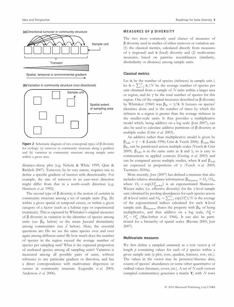
We distinguish two types of b diversity: turnover and

variation (Fig. 2; see also Vellend 2001). Both have clear

historical roots in Whittaker�s (1960, 1972) original concep-

tualization. The first is the notion of b diversity as turnover

(Fig. 2a). The essential idea here is to measure the change in

community structure from one sampling unit to another

along a spatial, temporal or environmental gradient. By

�change in community structure�, we mean a change in the

identity, relative abundance, biomass and ⁄ or cover of

individual species. Questions associated with turnover

include: How many new species are encountered along a

gradient and how many that were initially present are now

lost? What proportion of the species encountered is not

shared when we move from one unit to the next along this

gradient? Turnover can be expressed as a rate, as in a

30

15

20

25

0

5

10No.

of

pape

rs

Figure 1 Plot showing the number of peer-reviewed articles

published in the primary literature having �beta diversity� in their

title for each year from 1974 to 2009, based on ISIs Web of Science

database (note: this also includes titles that have used the greek

letter representation �b diversity�).

2 M. J. Anderson et al. Idea and Perspective


distance–decay plot (e.g. Nekola & White 1999; Qian &

Ricklefs 2007). Turnover, by its very nature, requires one to

define a specific gradient of interest with directionality. For

example, the rate of turnover in an east–west direction

might differ from that in a north–south direction (e.g.

Harrison et al. 1992).

The second type of b diversity is the notion of variation in

community structure among a set of sample units (Fig. 2b)

within a given spatial or temporal extent, or within a given

category of a factor (such as a habitat type or experimental

treatment). This is captured by Whittaker�s original measures

of b diversity as variation in the identities of species among

units (see bW below) or the mean Jaccard dissimilarity

among communities (see �d below). Here, the essential

questions are: Do we see the same species over and over

again among different units? By how much does the number

of species in the region exceed the average number of

species per sampling unit? What is the expected proportion

of unshared species among all sampling units? Variation is

measured among all possible pairs of units, without

reference to any particular gradient or direction, and has

a direct correspondence with multivariate dispersion or

variance in community structure (Legendre et al. 2005;

Anderson et al. 2006).

M E A S U R E S O F b D I V E R S I T Y

The two most commonly used classes of measures of

b diversity used in studies of either turnover or variation are:

(1) the classical metrics, calculated directly from measures

of c (regional) and a (local) diversity and (2) multivariate

measures, based on pairwise resemblances (similarity,

dissimilarity or distance) among sample units.

Classical metrics

Let ai be the number of species (richness) in sample unit i,

let �a ¼PN

i¼1 ai=N be the average number of species per

unit obtained from a sample of N units within a larger area

or region, and let c be the total number of species for this

region. One of the original measures described as b diversity

by Whittaker (1960) was bW ¼ c=�a. It focuses on species�identities alone and is the number of times by which the

richness in a region is greater than the average richness in

the smaller-scale units. It thus provides a multiplicative

model which, being additive on a log scale (Jost 2007), can

also be used to calculate additive partitions of b diversity at

multiple scales (Crist et al. 2003).

An additive rather than multiplicative model is given by

bAdd ¼ c� �a (Lande 1996; Crist & Veech 2006). bAdd, like

bW, can be partitioned across multiple scales (Veech & Crist

2009). bAdd is in the same units as �a and c, so is easy to

communicate in applied contexts (Gering et al. 2003) and

can be compared across multiple studies, when �a and bAdd

are expressed as proportions of c (Veech et al. 2003;

Tuomisto 2010a).

More recently, Jost (2007) has defined a measure that also

includes relative abundance information: bShannon = Hc ⁄ Ha,

where Hc ¼ expðH 0pooledÞ is an exponentiated Shannon–

Wiener index (i.e. effective diversity) for the c-level sample

unit (obtained by pooling abundances for each species across

all a-level units) and Ha ¼PN

i¼1 expðH 0i Þ=N is the average

of the exponentiated indices calculated for each a-level

sample unit. bShannon shares the property with bW of being

multiplicative, and thus additive on a log scale, H 0b ¼H 0c �H 0a (MacArthur et al. 1966). It can also be parti-

tioned for a hierarchy of spatial scales (Ricotta 2005; Jost

2007).

Multivariate measures

We first define a sampled community as a row vector y of

length p containing values for each of p species within a

given sample unit (a plot, core, quadrat, transect, tow, etc.).

The values in the vector may be presence ⁄ absence data,

counts of species� abundances or some other quantitative or

ordinal values (biomass, cover, etc.). A set of N such vectors

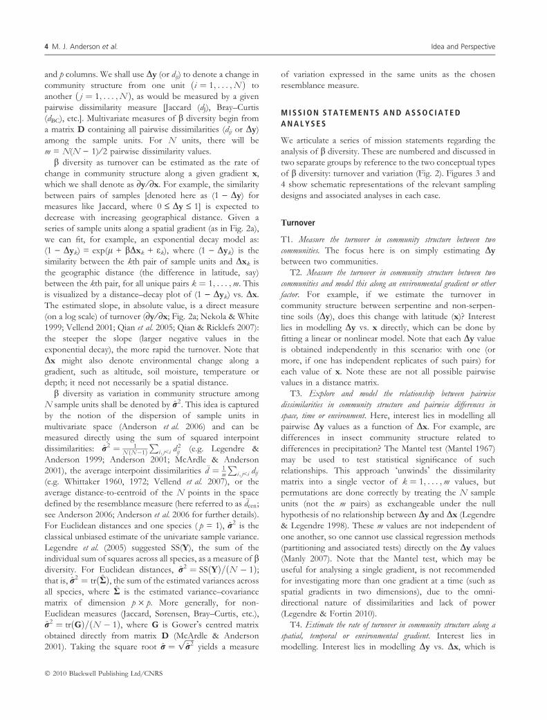
(sampled communities) generates a matrix Y, with N rows

(a) Directional turnover in community structure

Sample unit

Transect

Spatial, temporal or environmental gradient

(b) Variation in community structure (non-directional)

Sample unit

Spatial extentof sampling area

Figure 2 Schematic diagram of two conceptual types of b diversity

for ecology: (a) turnover in community structure along a gradient

and (b) variation in community structure among sample units

within a given area.

Idea and Perspective Roadmap for beta diversity 3


and p columns. We shall use Dy (or dij) to denote a change in

community structure from one unit ði ¼ 1; . . . ;N Þ to

another ð j ¼ 1; . . . ;N Þ, as would be measured by a given

pairwise dissimilarity measure [Jaccard (dJ), Bray–Curtis

(dBC), etc.]. Multivariate measures of b diversity begin from

a matrix D containing all pairwise dissimilarities (dij or Dy)

among the sample units. For N units, there will be

m = N(N ) 1) ⁄ 2 pairwise dissimilarity values.

b diversity as turnover can be estimated as the rate of

change in community structure along a given gradient x,

which we shall denote as ¶y ⁄ ¶x. For example, the similarity

between pairs of samples [denoted here as (1 ) Dy) for

measures like Jaccard, where 0 £ Dy £ 1] is expected to

decrease with increasing geographical distance. Given a

series of sample units along a spatial gradient (as in Fig. 2a),

we can fit, for example, an exponential decay model as:

(1 ) Dyk) = exp(l + bDxk + ek), where (1 ) Dyk) is the

similarity between the kth pair of sample units and Dxk is

the geographic distance (the difference in latitude, say)

between the kth pair, for all unique pairs k ¼ 1; . . . ;m. This

is visualized by a distance–decay plot of (1 ) Dyk) vs. Dx.

The estimated slope, in absolute value, is a direct measure

(on a log scale) of turnover (¶y ⁄ ¶x; Fig. 2a; Nekola & White

1999; Vellend 2001; Qian et al. 2005; Qian & Ricklefs 2007):

the steeper the slope (larger negative values in the

exponential decay), the more rapid the turnover. Note that

Dx might also denote environmental change along a

gradient, such as altitude, soil moisture, temperature or

depth; it need not necessarily be a spatial distance.

b diversity as variation in community structure among

N sample units shall be denoted by r2. This idea is captured

by the notion of the dispersion of sample units in

multivariate space (Anderson et al. 2006) and can be

measured directly using the sum of squared interpoint

dissimilarities: r2 ¼ 1N ðN�1Þ

Pi; j<i d 2

ij (e.g. Legendre &

Anderson 1999; Anderson 2001; McArdle & Anderson

2001), the average interpoint dissimilarities �d ¼ 1m

Pi; j<i dij

(e.g. Whittaker 1960, 1972; Vellend et al. 2007), or the

average distance-to-centroid of the N points in the space

defined by the resemblance measure (here referred to as �dcen;

see Anderson 2006; Anderson et al. 2006 for further details).

For Euclidean distances and one species ( p = 1), r2 is the

classical unbiased estimate of the univariate sample variance.

Legendre et al. (2005) suggested SS(Y), the sum of the

individual sum of squares across all species, as a measure of bdiversity. For Euclidean distances, r2 ¼ SSðYÞ=ðN � 1Þ;that is, r2 ¼ trðRÞ, the sum of the estimated variances across

all species, where R is the estimated variance–covariance

matrix of dimension p · p. More generally, for non-

Euclidean measures (Jaccard, Sørensen, Bray–Curtis, etc.),

r2 ¼ trðGÞ=ðN � 1Þ, where G is Gower�s centred matrix

obtained directly from matrix D (McArdle & Anderson

2001). Taking the square root r ¼ffiffiffiffiffir2p

yields a measure

of variation expressed in the same units as the chosen

resemblance measure.

M I S S I O N S T A T E M E N T S A N D A S S O C I A T E D

A N A L Y S E S

We articulate a series of mission statements regarding the

analysis of b diversity. These are numbered and discussed in

two separate groups by reference to the two conceptual types

of b diversity: turnover and variation (Fig. 2). Figures 3 and

4 show schematic representations of the relevant sampling

designs and associated analyses in each case.

Surnover

T1. Measure the turnover in community structure between two

communities. The focus here is on simply estimating Dy

between two communities.

T2. Measure the turnover in community structure between two

communities and model this along an environmental gradient or other

factor. For example, if we estimate the turnover in

community structure between serpentine and non-serpen-

tine soils (Dy), does this change with latitude (x)? Interest

lies in modelling Dy vs. x directly, which can be done by

fitting a linear or nonlinear model. Note that each Dy value

is obtained independently in this scenario: with one (or

more, if one has independent replicates of such pairs) for

each value of x. Note these are not all possible pairwise

values in a distance matrix.

T3. Explore and model the relationship between pairwise

dissimilarities in community structure and pairwise differences in

space, time or environment. Here, interest lies in modelling all

pairwise Dy values as a function of Dx. For example, are

differences in insect community structure related to

differences in precipitation? The Mantel test (Mantel 1967)

may be used to test statistical significance of such

relationships. This approach �unwinds� the dissimilarity

matrix into a single vector of k ¼ 1; . . . ;m values, but

permutations are done correctly by treating the N sample

units (not the m pairs) as exchangeable under the null

hypothesis of no relationship between Dy and Dx (Legendre

& Legendre 1998). These m values are not independent of

one another, so one cannot use classical regression methods

(partitioning and associated tests) directly on the Dy values

(Manly 2007). Note that the Mantel test, which may be

useful for analysing a single gradient, is not recommended

for investigating more than one gradient at a time (such as

spatial gradients in two dimensions), due to the omni-

directional nature of dissimilarities and lack of power

(Legendre & Fortin 2010).

T4. Estimate the rate of turnover in community structure along a

spatial, temporal or environmental gradient. Interest lies in

modelling. Interest lies in modelling Dy vs. Dx, which is



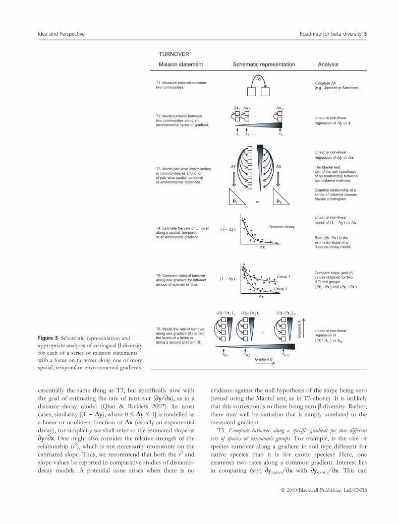
essentially the same thing as T3, but specifically now with

the goal of estimating the rate of turnover (¶y ⁄ ¶x), as in a

distance–decay model (Qian & Ricklefs 2007). In most

cases, similarity [(1 ) Dy), where 0 £ Dy £ 1] is modelled as

a linear or nonlinear function of Dx (usually an exponential

decay); for simplicity we shall refer to the estimated slope as

¶y ⁄ ¶x. One might also consider the relative strength of the

relationship (r2), which is not necessarily monotonic on the

estimated slope. Thus, we recommend that both the r2 and

slope values be reported in comparative studies of distance–

decay models. A potential issue arises when there is no

evidence against the null hypothesis of the slope being zero

(tested using the Mantel test, as in T3 above). It is unlikely

that this corresponds to there being zero b diversity. Rather,

there may well be variation that is simply unrelated to the

measured gradient.

T5. Compare turnover along a specific gradient for two different

sets of species or taxonomic groups. For example, is the rate of

species turnover along a gradient in soil type different for

native species than it is for exotic species? Here, one

examines two rates along a common gradient. Interest lies

in comparing (say) ¶ynative ⁄ ¶x with ¶yexotic ⁄ ¶x. This can

TURNOVER

Figure 3 Schematic representation and

appropriate analyses of ecological b diversity

for each of a series of mission statements

with a focus on turnover along one or more

spatial, temporal or environmental gradients.



be done visually by looking at plots of the models, but

note that lack of independence among the Dy values

precludes the use of a classical ANCOVA. A test of the null

hypothesis of no difference in the slopes may be done,

however, by randomly re-allocating the species into the

groups (native vs. exotic), but leaving x fixed, to generate

a null distribution for the difference in slopes. The

concept of halving distance (Soininen et al. 2007) might

also be considered here.

T6. Explore and model the rate of turnover along a gradient across

different levels of another factor or along another gradient. For

example, is the rate of turnover in marine benthic

invertebrates along a depth gradient different for different

latitudes or through time? Here, the response variable is

turnover (¶y ⁄ ¶x) along a chosen gradient, and one may

model this in response to a complex experimental design

(e.g. with several factors and their interactions) or sets of

other continuous predictor variables (e.g. temperature,

salinity, nutrients, etc.). There are no limitations on the

types of models that could be used here (linear or nonlinear,

classical or nonparametric), provided independent (and

preferably replicated) values of ¶y ⁄ ¶x are estimated at each

point within the sampling design. For example, separate

independent estimates of turnover along a depth gradient

¶y ⁄ ¶xdepth may be modelled as a function of latitude,

substratum type and ⁄ or nutrients.

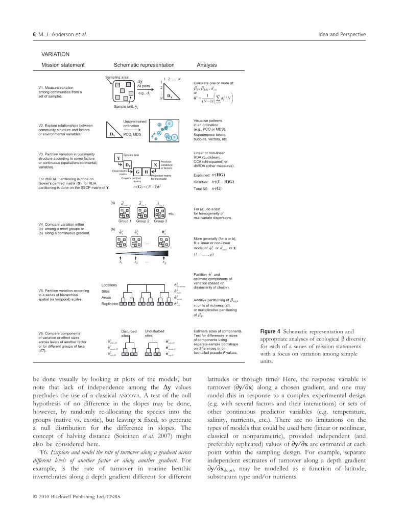
Figure 4 Schematic representation and

appropriate analyses of ecological b diversity

for each of a series of mission statements

with a focus on variation among sample

units.



Variation

V1. Measure the variation in community structure among a set of

samples. Here, the focus is simply on estimating variation,

which can be achieved by calculating one or more of the

classical (bW, bAdd) or multivariate measures discussed

above ( �d , r2 or �dcen, on the basis of a chosen resemblance

measure).

V2. Explore the relationship between community structure and

some factor(s) or variable(s) of interest. Here, interest lies in

visualizing the potential relationship of Y vs. x (a single

variable) or X (several continuous variables or indicators of

factors). The factor(s) or variable(s) of interest may be

temporal, spatial or environmental from an observational

survey, or they may be experimentally manipulated treat-

ments. Unconstrained ordination such as principal coordi-

nates analysis or non-metric multi-dimensional scaling

(MDS) can be used to examine patterns in a multivariate

data cloud on the basis of a chosen resemblance measure.

Potential relationships with X are explored by superimpos-

ing labels on points (for groups), bubbles (for quantitative

variables) or vectors (showing multiple linear relationships

with axes). This is called indirect gradient analysis (e.g. ter

Braak 1987) and covers a plethora of methods. Importantly,

differences in the relative sizes of multivariate dispersions

for different groups can be visualized on unconstrained

ordination plots (e.g. Anderson 2006; Chase 2007, 2010).

V3. Partition the variation in community structure in response to

some quantitative variables or factors (spatial, temporal, environmen-

tal, experimental). This is achieved by modelling Y in terms of

x (or X). The total variation in Y is r2, but interest lies here

specifically in determining how much of this variation is

explained by functions of other variables (and their overlap

if they are non-independent). For example, how much of

the spatial variation in communities of herbs is explained by

the factors of fire frequency, fencing to prevent grazing, and

their interaction? If the partitioning involves a fixed factor

(e.g. disturbed vs. undisturbed treatments in an experiment),

then the component of variation for that factor is

interpreted as an effect size. r2 can be partitioned directly

according to multi-factor experimental or hierarchical

sampling designs (using PERMANOVA; Anderson 2001;

Anderson et al. 2008) or continuous environmental or

spatial gradients [using redundancy analysis (RDA), canon-

ical correspondence analysis (CCA) or distance-based

redundancy analysis (dbRDA); Borcard et al. 1992; Legendre

& Anderson 1999; McArdle & Anderson 2001; Anderson

et al. 2008]. dbRDA on Euclidean distances yields a classical

RDA, as tr(G) = SS(Y) in that case, while dbRDA on chi-

squared distances yields results very close to CCA (ter Braak

1986). Partitioning in the space of the chi-squared, Hellinger

or chord measures can also be obtained by RDA on a simple

transformation of the values in matrix Y (Legendre &

Gallagher 2001). Advantages to using RDA, thus working

with SS(Y), on either raw or transformed data include the

direct interpretability of ordination axes in terms of the

original variables and the computational speed of partition-

ing a p · p matrix of sums of squares and cross products

(SSCP) rather than the N · N matrix (G) if N � p.

Although the direct link to original Y variables is broken

once a dissimilarity matrix D has been formed, dbRDA

allows much more flexibility in the choice of resemblance

measure (Jaccard, Sørensen, Bray–Curtis, etc.), and yields a

faster core algorithm when p > N. Also, dbRDA does not

require calculation of principal coordinates or corrections

for negative eigenvalues, but directly partitions matrix G (see

Fig. 4; McArdle & Anderson 2001; Anderson et al. 2008).

V4. Compare variation in community structure among several levels

of a factor (categorical) or along a gradient (continuous). For

example, does the degree of variation in species� identities

change with depth? If one has n replicate sample units

within each of g levels of a factor (N = g · n) then we can

formally test the null hypothesis of homogeneity of

multivariate dispersions (Anderson 2006; Anderson et al.

2006, 2008). For example, we can compare �dcen for shallow

vs. deep sites. A statistical comparison of r2‘ values

ð‘ ¼ 1; . . . ; gÞ among groups could also be performed

using a separate-sample bootstrap, as described by Manly

(2007) for univariate data. Furthermore, if groups occur

along a gradient (e.g. in a series of depth strata), then we

may model values of �d , �dcen or r2 vs. depth (x). More

complex designs are also possible where multiple values of

r2 have been obtained along more than one gradient or

factor.

V5. Partition the variation in community structure according to a

series of additive hierarchical spatial scales. When there is more

than one spatial scale of interest, a relevant sampling design

would have hierarchical random factors at a number of

scales within a region, such as locations, sites within

locations and replicates within sites. Here, one would

calculate (for example): r2total ¼ r2

replicates þ r2sites þ r2

locations.

This yields additive components of variation. Estimators for

these can be calculated from mean squares and tested using

permutation methods as pseudo multivariate variance

components (Anderson et al. 2005), direct analogues to the

unbiased univariate ANOVA estimators (Searle et al. 1992).

Although partitioning to obtain sums of squares for each

factor is calculated from SS(Y) (in RDA) or tr(G) (in

dbRDA or PERMANOVA), the actual components of variation

(r2, which take into account degrees of freedom), are

required for making valid comparisons. For analyses of one

variable using Euclidean distances, these are the classical

univariate variance components (Searle et al. 1992). Notably,

unbiased estimators for these components are derived from

expectations of mean squares, which will be specific not just to

the individual component being estimated, but also to the



particular model in which they are found; they will depend

especially on the nature of any nested structures and

whether factors included in the model are to be treated

as fixed or random (Searle et al. 1992; Anderson et al.

2008). Partitioning might also be done as c = a +

breplicates + bsites + blocations (Crist et al. 2003; Crist & Veech

2006). Note that a is a measure of diversity within a sample,

which is not discussed explicitly here in the form of a

variance component, but see Pelissier & Couteron (2007).

Thus, c is not the same as r2 because c includes a. Similarly,

a multiplicative hierarchical partition is: c = a · breplicates ·bsites · blocations. Either an additive or multiplicative parti-

tioning of these classical measures can be calculated, with

statistical tests of null hypotheses (Veech & Crist 2009).

Finally, for modelling scales of variation along a continuum,

rather than hierarchically, one may consider doing an

analysis using principal coordinate analysis of neighbour

matrices (PCNM) (Dray et al. 2006; Legendre et al. 2009).

V6. Compare individual components of variation in community

structure from a partitioning across some other factor or variable of

interest. For example, how does the partitioning of r2 change

when we look at disturbed vs. undisturbed environments?

Specifically, we may wish to test for a difference in the sizes

of individual components; is b diversity at the scale of sites,

r2sites, significantly larger (or smaller) in disturbed than in

undisturbed environments? A direct multivariate analogue

to the univariate two-tailed F-ratios (Underwood 1991)

could be used to compare such components, but with

P-values obtained using bootstrapping (Davison & Hinkley

1997; Manly 2007). Components could also be compared

across multiple levels of other factors, with formal tests for

differences obtained using bootstrapping, as has been done

to compare univariate variance components (Terlizzi et al.

2005).

V7. Compare components of variation in community structure for

different sets of species or taxonomic groups. An example here

might be: is b diversity for annelids at the scale of sites, r2sites,

larger (or smaller) than that for molluscs? This is a bit like

comparing components across levels of another factor (V6).

Components of variation for different groups of organisms

can be calculated and compared directly (Anderson et al.

2005). Care is needed, however, in designing formal tests; if

components for different groups are calculated from the

same dataset they may not be independent.

K E Y P R O P E R T I E S O F P A I R W I S E R E S E M B L A N C E

M E A S U R E S F O R E C O L O G I C A L I N T E R P R E T A T I O N

Pairwise dissimilarities form the basis of multivariate

analyses of b diversity. Different measures have different

properties. They emphasize different aspects of community

data and therefore can yield very different results. Rather

than being a handicap, we advocate that this plurality be

used as an advantage. Comparing and contrasting the results

obtained from judicious use of a suite of directly interpret-

able measures can yield important ecological insights into

the actual nature of patterns in b diversity. Analyses

performed using different measures correspond to different

underlying ecological hypotheses.

We provide here a key to the essential properties

associated with the most commonly used measures in the

ecological analysis of community data (Table 1; Fig. 5). See

Legendre & Legendre (1998), Koleff et al. (2003) and

Tuomisto (2010a,b) for more.

Presence ⁄ absence vs. relative abundance information

The first important conceptual distinction (Table 1; Fig. 5)

is between measures that use identities of species only

(presence ⁄ absence data), vs. those that include abundance

(or relative abundance or biomass or other) information as

well. The classical measures of bW and bAdd do not include

relative abundance information, but bShannon does. This

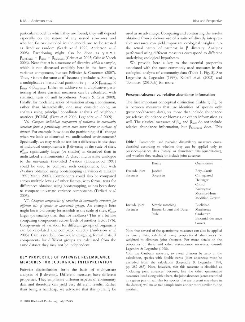
Table 1 Commonly used pairwise dissimilarity measures cross-

classified according to whether they can be applied only to

presence–absence data (binary) or abundance data (quantitative),

and whether they exclude or include joint absences

Binary Quantitative

Exclude joint

absences

Jaccard

Sørensen

Bray–Curtis

Chi squared

Hellinger

Chord

Kulczynski

Morisita-Horn

Modified Gower

Include joint

absences

Simple matching

Baroni-Urbani and Buser

Yule

Euclidean

Manhattan

Canberra*

Binomial deviance

Gower

Note that several of the quantitative measures can also be applied

to binary data, calculated using proportional abundances or

weighted to eliminate joint absences. For more details on the

properties of these and other resemblance measures, consult

Legendre & Legendre (1998).

*For the Canberra measure, to avoid division by zero in the

calculation, species with double zeros (joint absences) must be

excluded from the calculation (Legendre & Legendre 1998,

pp. 282–283). Note, however, that this measure is classified as

�including joint absences� because, like the other quantitative

measures listed along with it here, the joint absences (zeros recorded

in a given pair of samples for species that are present elsewhere in

the dataset) will make two sample units appear more similar to one

another.



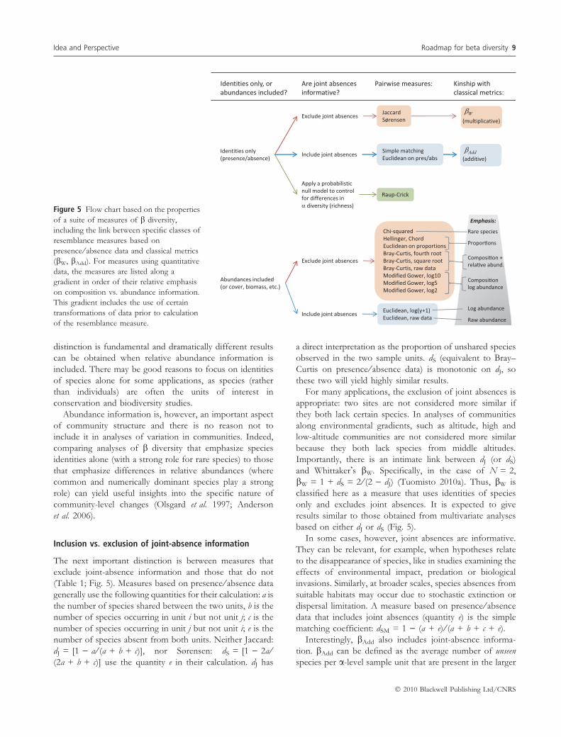
distinction is fundamental and dramatically different results

can be obtained when relative abundance information is

included. There may be good reasons to focus on identities

of species alone for some applications, as species (rather

than individuals) are often the units of interest in

conservation and biodiversity studies.

Abundance information is, however, an important aspect

of community structure and there is no reason not to

include it in analyses of variation in communities. Indeed,

comparing analyses of b diversity that emphasize species

identities alone (with a strong role for rare species) to those

that emphasize differences in relative abundances (where

common and numerically dominant species play a strong

role) can yield useful insights into the specific nature of

community-level changes (Olsgard et al. 1997; Anderson

et al. 2006).

Inclusion vs. exclusion of joint-absence information

The next important distinction is between measures that

exclude joint-absence information and those that do not

(Table 1; Fig. 5). Measures based on presence ⁄ absence data

generally use the following quantities for their calculation: a is

the number of species shared between the two units, b is the

number of species occurring in unit i but not unit j; c is the

number of species occurring in unit j but not unit i; e is the

number of species absent from both units. Neither Jaccard:

dJ = [1 ) a ⁄ (a + b + c)], nor Sørensen: dS = [1 ) 2a ⁄(2a + b + c)] use the quantity e in their calculation. dJ has

a direct interpretation as the proportion of unshared species

observed in the two sample units. dS (equivalent to Bray–

Curtis on presence ⁄ absence data) is monotonic on dJ, so

these two will yield highly similar results.

For many applications, the exclusion of joint absences is

appropriate: two sites are not considered more similar if

they both lack certain species. In analyses of communities

along environmental gradients, such as altitude, high and

low-altitude communities are not considered more similar

because they both lack species from middle altitudes.

Importantly, there is an intimate link between dJ (or dS)

and Whittaker�s bW. Specifically, in the case of N = 2,

bW = 1 + dS = 2 ⁄ (2 ) dJ) (Tuomisto 2010a). Thus, bW is

classified here as a measure that uses identities of species

only and excludes joint absences. It is expected to give

results similar to those obtained from multivariate analyses

based on either dJ or dS (Fig. 5).

In some cases, however, joint absences are informative.

They can be relevant, for example, when hypotheses relate

to the disappearance of species, like in studies examining the

effects of environmental impact, predation or biological

invasions. Similarly, at broader scales, species absences from

suitable habitats may occur due to stochastic extinction or

dispersal limitation. A measure based on presence ⁄ absence

data that includes joint absences (quantity e) is the simple

matching coefficient: dSM = 1 ) (a + e) ⁄ (a + b + c + e).

Interestingly, bAdd also includes joint-absence informa-

tion. bAdd can be defined as the average number of unseen

species per a-level sample unit that are present in the larger

Figure 5 Flow chart based on the properties

of a suite of measures of b diversity,

including the link between specific classes of

resemblance measures based on

presence ⁄ absence data and classical metrics

(bW, bAdd). For measures using quantitative

data, the measures are listed along a

gradient in order of their relative emphasis

on composition vs. abundance information.

This gradient includes the use of certain

transformations of data prior to calculation

of the resemblance measure.



c-level unit. Although bAdd = ½(b + c) when N = 2, the

inclusion of joint-absence information (e) in bAdd is explicit

when one considers the contribution (b*) of any two sample

units towards bAdd when N > 2, namely, b* = e + ½

(b + c). In addition, bAdd when N = 2 is also a function of

Euclidean distance (dEuc) when calculated on pres-

ence ⁄ absence data, namely bAdd = ½(dEuc)2 (Tuomisto

2010a). Thus, results obtained using bAdd are expected to

give similar results to multivariate analyses based on dSM.

There are many ecological dissimilarity measures that

include relative abundance information (Legendre & Legen-

dre 1998; Chao et al. 2005; Anderson et al. 2006; Clarke et al.

2006), and most of these exclude joint absences (Table 1;

Fig. 5). Measures in this class include Bray–Curtis, one of

the most popular abundance-based metrics (Bray & Curtis

1957; Clarke et al. 2006), along with modified Gower

(Anderson et al. 2006), chi squared (having a kinship with

correspondence analysis, ter Braak 1985; Legendre &

Legendre 1998) and Hellinger (Rao 1995; Legendre &

Gallagher 2001).

Joint-absence information may be relevant to include,

however, if hypotheses focus on phenomena that can cause

changes in total (rather than proportional) abundances,

biomass or cover, such as in studies of productivity,

upwelling, disturbance or predation. Measures in this

category include Euclidean distance and the Manhattan

measure. When analysing counts of abundances (which are

often overdispersed), such distances are usually calculated

on log( y + 1)-transformed data. Figure 5 shows schemat-

ically how changes in the choice of measure, as well as the

transformation used, will alter the relative importance of

composition, relative or raw abundance information in

terms of their contribution towards the results obtained, as a

continuum.

Probabilistic measures under a null model: accountingfor differences in a

Pairwise measures of dissimilarity, such as dJ or dS, will

depend to some extent on the number of species in the

sample units. When there is a large difference in richness

between two samples, the corresponding dissimilarity

should automatically increase, as the potential for overlap

(quantity a) is reduced (Koleff et al. 2003). This issue has led

to various attempts to remove the effect of differences in afrom measures of b diversity (Lennon et al. 2001).

One way to remove effects of a on b is to use a null-

modelling approach. For example, Raup & Crick (1979)

proposed a probabilistic resemblance measure, dRC, which is

interpretable as the probability that two sample units share

fewer species than expected for samples drawn randomly

from the species pool, given their existing differences in

richness (see also Chase 2007, 2010; Vellend et al. 2007).

More specifically, let a1 and a2 be the respective number of

species in each of two sample units. One generates a null

distribution of dJ from repeated random draws of a1 and a2

species from the species pool (c), with the probability of

drawing each species being its proportional occurrence in all

sample units. dRC is the proportion of pairs of communities

generated under the null model that share the same number

or more species in common than the original sample units.

Thus, dRC measures b diversity while conditioning on a.

Although dRC still depends on c (a topic for further

research), analyses based on dRC allow one to identify

changes in b diversity (increases in variation as measured by

dJ) that are driven by changes in a alone (Vellend et al.

2007). By teasing out the a-driven component of b diversity

for presence ⁄ absence data, the probabilistic null model

implemented by dRC yields a very useful tool that, especially

when coupled with well-designed experiments, can help to

unravel the underlying mechanisms generating variation in

ecological communities (Chase 2010).

R E V E A L I N G T H E N A T U R E O F C H A N G E S I N bD I V E R S I T Y U S I N G D I F F E R E N T M E A S U R E S :

A C A S E S T U D Y

A full set of analyses for all of the mission statements is

beyond the scope of this article, hence we focus here on an

illustration of how multiple analyses of a given dataset can

yield deeper insights than any one analysis. Rather than

choosing a single measure of b diversity, we recognize that

communities have a variety of ecological properties of

interest, and we advocate using a suite of measures, each

driven by specific hypotheses. This approach can directly

reveal the nature of changes in community structure. This is

not to suggest that all available measures should always be

used. Rather it is to compare results obtained using a subset

of contrasting measures that focus on different properties,

so meaningful interpretations can follow.

We illustrate this approach by analysing observational

data where the mission is to compare variation among

several groups of samples (V4a) in response to a distur-

bance. This is one of the most common and general mission

statements in ecological studies and this case study

purposefully exemplifies strong contrasts in results with

choice of resemblance measure. The percentage cover of

75 species of coral was measured along each of 10 transects

on reefs in the Tikus Islands, Indonesia, in each of several

years from 1981 to 1988 (Warwick et al. 1990; data are

provided in Appendix S1 in Supporting Information). In

1982, there was a dramatic bleaching of the corals

(disturbance), triggered by El Nino. We examined commu-

nity variation for n = 10 transects in three years: 1981, 1983

and 1985. Results differed dramatically for different

measures (Fig. 6; Table 2), but several classes of outcomes



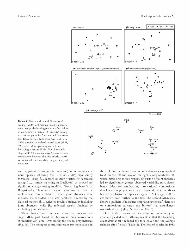
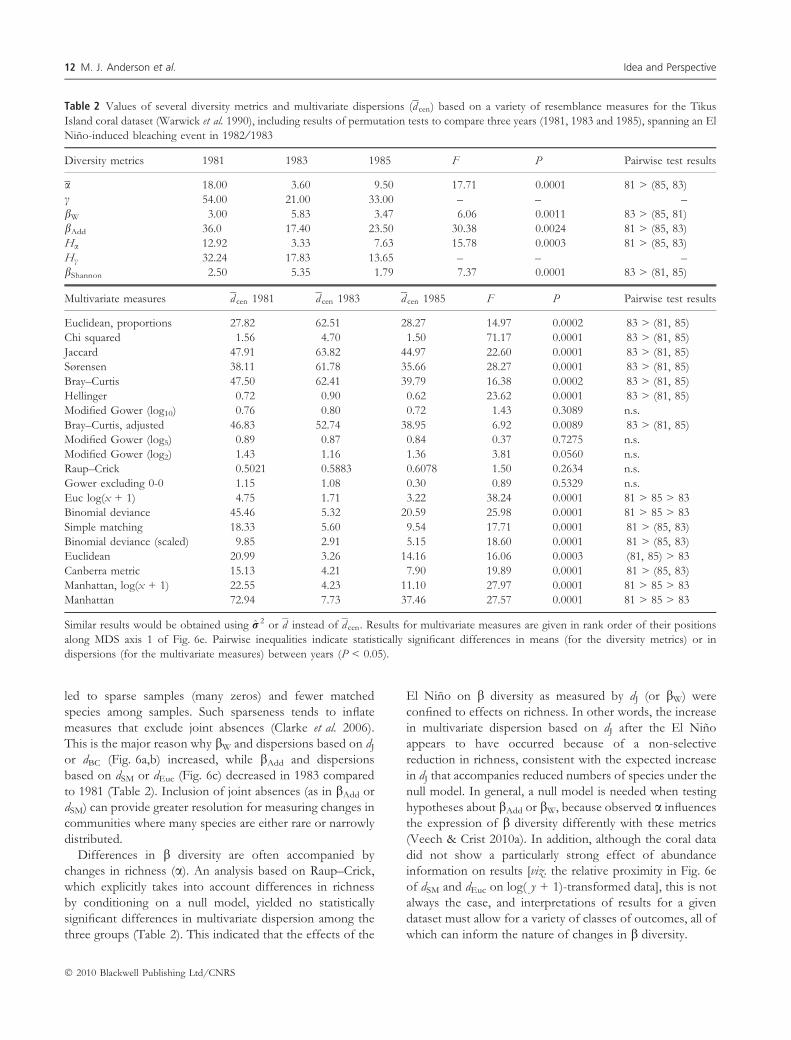
were apparent. b diversity (as variation) in communities of

coral species following the El Nino (1983) significantly

increased (using bW, Jaccard or Bray–Curtis), or decreased

(using bAdd, simple matching or Euclidean) or showed no

significant change (using modified Gower log base 5, or

Raup–Crick). There was a clear dichotomy between the

multivariate results obtained when joint absences were

included vs. excluded. This was paralleled directly by the

classical metrics: bAdd reflected results obtained by including

joint absences, while bW reflected results obtained by

excluding joint absences.

These classes of outcomes can be visualized in a second-

stage MDS plot based on Spearman rank correlations

(Somerfield & Clarke 1995) among the dissimilarity matrices

(Fig. 6e). The strongest contrast in results for these data is in

the exclusion vs. the inclusion of joint absences, exemplified

by dJ on the left and dSM on the right (along MDS axis 1),

which differ only in this respect. Exclusion of joint absences

led to significantly greater observed variability post-distur-

bance. Measures emphasizing proportional composition

(Euclidean on proportions, or chi squared, which tends to

heavily emphasize rare species, Legendre & Gallagher 2001)

are shown even further to the left. The second MDS axis

shows a gradient of measures emphasizing species� identities

or composition (towards the bottom) vs. abundances

(towards the top) (Fig. 6e; see also Fig. 5).

One of the reasons that including or excluding joint

absences yielded such differing results is that the bleaching

event dramatically reduced the total cover and the average

richness (�a) of corals (Table 2). The loss of species in 1983

1981 1983 1985(a) Jaccard (b) Bray Curtis

Stress: 0.15 Stress: 0.15

(c) Euclidean distance, ln(x + 1)-transformed data (d) Modified Gower (log base 5)

Stress: 0.08 Stress: 0.17

(e) 2nd-stage MDS

MG.10MG.5

MG.2

Gow.ex

Euc

Stress: 0.04

J

BC BCadj

Euc.p

Euc.log

ChiH

Man

Man.log

CanBdev.s

Sor

SM

Bdev

Figure 6 Non-metric multi-dimensional

scaling (MDS) ordinations based on several

measures (a–d) showing patterns of variation

in community structure (b diversity) among

n = 10 sample units for the coral data from

the Tikus Islands, Indonesia (Warwick et al.

1990) sampled in each of several years (1981,

1983 and 1985), spanning an El Nino

bleaching event in 1982 ⁄ 1983. A second-

stage MDS (e) shows relative Spearman rank

correlations between the dissimilarity matri-

ces obtained for these data using a variety of

measures.



led to sparse samples (many zeros) and fewer matched

species among samples. Such sparseness tends to inflate

measures that exclude joint absences (Clarke et al. 2006).

This is the major reason why bW and dispersions based on dJ

or dBC (Fig. 6a,b) increased, while bAdd and dispersions

based on dSM or dEuc (Fig. 6c) decreased in 1983 compared

to 1981 (Table 2). Inclusion of joint absences (as in bAdd or

dSM) can provide greater resolution for measuring changes in

communities where many species are either rare or narrowly

distributed.

Differences in b diversity are often accompanied by

changes in richness (a). An analysis based on Raup–Crick,

which explicitly takes into account differences in richness

by conditioning on a null model, yielded no statistically

significant differences in multivariate dispersion among the

three groups (Table 2). This indicated that the effects of the

El Nino on b diversity as measured by dJ (or bW) were

confined to effects on richness. In other words, the increase

in multivariate dispersion based on dJ after the El Nino

appears to have occurred because of a non-selective

reduction in richness, consistent with the expected increase

in dJ that accompanies reduced numbers of species under the

null model. In general, a null model is needed when testing

hypotheses about bAdd or bW, because observed a influences

the expression of b diversity differently with these metrics

(Veech & Crist 2010a). In addition, although the coral data

did not show a particularly strong effect of abundance

information on results [viz. the relative proximity in Fig. 6e

of dSM and dEuc on log( y + 1)-transformed data], this is not

always the case, and interpretations of results for a given

dataset must allow for a variety of classes of outcomes, all of

which can inform the nature of changes in b diversity.

Table 2 Values of several diversity metrics and multivariate dispersions (d cen) based on a variety of resemblance measures for the Tikus

Island coral dataset (Warwick et al. 1990), including results of permutation tests to compare three years (1981, 1983 and 1985), spanning an El

Nino-induced bleaching event in 1982 ⁄ 1983

Diversity metrics 1981 1983 1985 F P Pairwise test results

a 18.00 3.60 9.50 17.71 0.0001 81 > (85, 83)

c 54.00 21.00 33.00 – – –

bW 3.00 5.83 3.47 6.06 0.0011 83 > (85, 81)

bAdd 36.0 17.40 23.50 30.38 0.0024 81 > (85, 83)

Ha 12.92 3.33 7.63 15.78 0.0003 81 > (85, 83)

Hc 32.24 17.83 13.65 – – –

bShannon 2.50 5.35 1.79 7.37 0.0001 83 > (81, 85)

Multivariate measures d cen 1981 d cen 1983 d cen 1985 F P Pairwise test results

Euclidean, proportions 27.82 62.51 28.27 14.97 0.0002 83 > (81, 85)

Chi squared 1.56 4.70 1.50 71.17 0.0001 83 > (81, 85)

Jaccard 47.91 63.82 44.97 22.60 0.0001 83 > (81, 85)

Sørensen 38.11 61.78 35.66 28.27 0.0001 83 > (81, 85)

Bray–Curtis 47.50 62.41 39.79 16.38 0.0002 83 > (81, 85)

Hellinger 0.72 0.90 0.62 23.62 0.0001 83 > (81, 85)

Modified Gower (log10) 0.76 0.80 0.72 1.43 0.3089 n.s.

Bray–Curtis, adjusted 46.83 52.74 38.95 6.92 0.0089 83 > (81, 85)



Raup–Crick 0.5021 0.5883 0.6078 1.50 0.2634 n.s.

Gower excluding 0-0 1.15 1.08 0.30 0.89 0.5329 n.s.

Euc log(x + 1) 4.75 1.71 3.22 38.24 0.0001 81 > 85 > 83

Binomial deviance 45.46 5.32 20.59 25.98 0.0001 81 > 85 > 83

Simple matching 18.33 5.60 9.54 17.71 0.0001 81 > (85, 83)

Binomial deviance (scaled) 9.85 2.91 5.15 18.60 0.0001 81 > (85, 83)

Euclidean 20.99 3.26 14.16 16.06 0.0003 (81, 85) > 83

Canberra metric 15.13 4.21 7.90 19.89 0.0001 81 > (85, 83)

Manhattan, log(x + 1) 22.55 4.23 11.10 27.97 0.0001 81 > 85 > 83

Manhattan 72.94 7.73 37.46 27.57 0.0001 81 > 85 > 83

Similar results would be obtained using r 2 or d instead of d cen. Results for multivariate measures are given in rank order of their positions

along MDS axis 1 of Fig. 6e. Pairwise inequalities indicate statistically significant differences in means (for the diversity metrics) or in

dispersions (for the multivariate measures) between years (P < 0.05).



C A U T I O N A R Y N O T E S

When discussing b diversity, clarity is needed regarding the

type of b diversity of interest: either turnover by reference

to a specific gradient or variation (Fig. 2). The sampling

design and ensuing analysis should reflect this (Figs 3 and

4). In addition, while a variety of measures may be used

advantageously in concert, results must be interpreted in

accordance with the ecological properties emphasized by

those measures.

Recently, b diversity was described as a �level 3

abstraction�, where one examines �variation in variation in

raw data� (Tuomisto & Ruokolainen 2006). Analyses of

quantities such as �dcen;‘ or models of r2‘ vs. x‘, as in missions

V4(a) or V4(b) above, are indeed analyses of how variation,

itself, is changing along a gradient or among regions.

However, the estimated variance of the dissimilarity values,

namely, r2d ¼ 1

ðm�1ÞP

i; j<i ðdij � �d Þ2 (Tuomisto & Ruokolai-

nen 2006) is not an interpretable measure of b diversity.

Simply put, the m = N(N ) 1) ⁄ 2 pairs of dissimilarity

values calculated from a set of N sample units are not

independent of one another. There are not (m ) 1) degrees

of freedom in the system as implied by this approach.

Unfortunately, the nature of the non-independence among

dij values for a given system of N points is not easy to

unravel for direct modelling purposes.

It has been suggested, furthermore, that multiple regres-

sion directly on dissimilarities can be used to �partition�variation in Dy, such as Dyk = l + b1Dxk + b2Dzk + ek,

where Dxk are (say) spatial distances and Dzk are environ-

mental distances. It is certainly possible to estimate

coefficients for this model, despite obvious violation of

the assumption of independence. However, the usual

agenda here is to see how much of the �variation� in Dy is

�explained� by space vs. the environment (Duivenvoorden

et al. 2002; Tuomisto et al. 2003). Unfortunately, there is no

clear sense in which the fitting of Dx to Dy has �controlled�for spatial relationships among the sample units, and the

meaning of the partial relationship of Dy with Dz, given Dx,

in terms of actual underlying spatial variation, is quite

unclear. Dutilleul et al. (2000) have demonstrated how the

Mantel correlation between distance matrices does not

accurately reflect known true correlations in underlying

variables, even for Euclidean distances on univariate normal

variables. Furthermore, Manly (2007, p. 215) has shown

how the effects of even simple spatial autocorrelation are

not removed by the regression of Dy on spatial distances

Dx. Thus, we do not advocate the use of multiple regression

directly on dissimilarity values (where the Dy values are

treated as a univariate response variable). The partial Mantel

approach (Smouse et al. 1986) has been known for some

time to be problematic for interpretation (e.g. Dutilleul et al.

2000; Legendre 2000; Legendre et al. 2005; Legendre &

Fortin 2010), in contrast with the simple Mantel test

which is a valid approach to relate two distance matrices

(Fig. 3, T3).

What is even more problematic is the use of partitioning

methods to make direct inferences regarding the relative

importance of underlying processes driving patterns in

b diversity (e.g. Duivenvoorden et al. 2002; Tuomisto et al.

2003). For example, researchers partition r2 into a portion

explained by a set of spatial variables (X), a portion

explained by a set of measured environmental variables (Z),

some overlap in what these two sets explain, and a residual

(unexplained) portion using RDA or dbRDA (Borcard et al.

1992; Legendre et al. 2009). This, in and of itself, is fine (see

V3 above). However, extreme caution is required when

interpreting results; it is sometimes claimed that the portion

attributable to �space� directly represents the relative

importance of �neutral processes� (sensu Hubbell 2001),

while that portion attributable to �environment� represents

the relative importance of �niche-based processes�. Unfor-

tunately, such conclusions cannot logically be inferred from

observational data (Underwood 1990). First, spatial struc-

ture in measured environmental variables (leading to

overlap in explained variation), precludes any logical

inference about whether processes were niche-based or

neutral. Also, apparently �spatial� portions interpreted as

�neutral� could simply have been due to unmeasured

environmental variables. For example, researchers often

neglect small-scale environmental variables when studying

ecological systems at large scales. This does not necessarily

mean that small-scale variation (appearing in the �spatial�portion when using the rather powerful method of PCNM,

for example, Dray et al. 2006) is driven by neutral

processes. Even variation attributed to environmental

variables alone might co-incidentally mirror patterns in

species that actually arose from neutral processes. Finally,

individual species vary in their degree of aggregation

(McArdle & Anderson 2004), so neutral processes should

yield spatial patterns at different scales for different species.

Thus, patterns in multivariate data are not easily interpreted

regarding the actual mechanisms at work for individual

species.

Methods of partitioning are helpful for uncovering

patterns and generating hypotheses (Underwood et al.

2000). To test potential mechanisms underlying observed

patterns, manipulative experiments isolating the factor(s) of

interest are required (Chase 2007, 2010). When controlled

experiments are not possible, a �toe-in-the-door� regarding

mechanisms might be obtained from ever-more-specific

null models (Chase 2007; Vellend et al. 2007), incorporating

explicit hypotheses regarding species pools (c) at a variety

of scales, or expectations of occupancies or relative

abundances. Insights can also be achieved through con-

trasting simultaneous analyses of observational data using



taxonomic, phylogenetic and functional b diversity (e.g.

Graham & Fine 2008; Swenson et al. 2010). In addition,

simulations of ecological processes under a variety

of stochastic and deterministic forces might be used to

identify plausible hypotheses for the mechanisms governing

b diversity.

C O N C L U S I O N S

We agree that researchers should be explicit about which

�b diversity� they are referring to, but we disagree that there

is only one �true b diversity� sensu Tuomisto (2010a).

Multivariate species data are information rich. Plurality in

the concept of b diversity can yield important ecological

insights when navigated well. By knowing the properties of

the measures being used and applying more than one, the

underlying ecological structures in the data generating

patterns in b diversity can be revealed, such as a selective

vs. non-selective loss of shared species, or an increase in the

variance of log-abundances.

We highlight the special utility of null models for

studying b diversity, which can eliminate the dependence

of b diversity on a diversity (e.g. the Raup–Crick measure)

and ⁄ or c diversity. Using the Raup–Crick measure also goes

some way (though not entirely) towards alleviating the

well-known problem of the classical (and most often used)

measures of b diversity (Whittaker, Jaccard and Sørensen),

which lose resolution for datasets having many samples that

share few species. This occurs in sparse datasets (often

encountered in studies of disturbance or predation) and also

in datasets spanning large spatial or temporal scales (as in

studies of latitudinal gradients or biogeography). The

appropriate species pool (c) to use in null models, especially

at broad scales, remains an important topic for future

research.

We consider that future studies of b diversity will lie

not just in the meaningful use of multiple approaches for

examining patterns, but also in the development of stronger

frameworks for assessing underlying processes. More

experiments directly testing mechanisms which generate

b diversity are needed. Where manipulative experiments are

not feasible (at large spatial or temporal scales), simulations,

multi-scale null models and con-joint analyses of abundance,

taxonomic, phylogenetic and functional information might

be used to narrow down potential instrumental models of

the mechanisms driving b diversity.

A C K N O W L E D G E M E N T S

This work was made possible by support from the National

Center for Ecological Analysis and Synthesis (NCEAS), Santa

Barbara, USA, through the activities of the working group

entitled �A synthesis of patterns, analyses, and mechanisms

of b diversity along ecological gradients�. M.J. Anderson was

also supported by a Royal Society of New Zealand Marsden

Grant (MAU0713). J.C. Stegen was supported by an NSF

Postdoctoral Fellowship in Bioinformatics (DBI-0906005).

N.J. Sanders was supported by grant DOE-PER DE-FG-02-

08ER64510. N.J.B. Kraft was supported by the NSERC

CREATE Training Program in Biodiversity Research. We

thank P. Legendre and an anonymous referee for their

comments on the manuscript.

R E F E R E N C E S

Anderson, M.J. (2001). A new method for non-parametric multi-

variate analysis of variance. Austral Ecol., 26, 32–46.

Anderson, M.J. (2006). Distance-based tests for homogeneity of

multivariate dispersions. Biometrics, 62, 245–253.

Anderson, M.J., Diebel, C.E., Blom, W.M. & Landers, T.J. (2005).

Consistency and variation in kelp holdfast assemblages: spatial

patterns of biodiversity for the major phyla at different taxo-

nomic resolutions. J. Exp. Mar. Biol. Ecol., 320, 35–56.

Anderson, M.J., Ellingsen, K.E. & McArdle, B.H. (2006). Multi-

variate dispersion as a measure of beta diversity. Ecol. Lett., 9,

683–693.

Anderson, M.J., Gorley, R.N. & Clarke, K.R. (2008). PERMA-

NOVA+ for PRIMER: Guide to Software and Statistical Methods.

PRIMER-E, Plymouth, UK.

Baselga, A. (2010). Multiplicative partition of true diversity yields

independent alpha and beta components; additive partition does

not. Ecology, 91, 1974–1981.

Borcard, D., Legendre, P. & Drapeau, P. (1992). Partialling out the

spatial component of ecological variation. Ecology, 73, 1045–1055.

ter Braak, C.J.F. (1985). Correspondence analysis of incidence and

abundance data: properties in terms of a unimodal response

model. Biometrics, 41, 859–873.

ter Braak, C.J.F. (1986). The analysis of vegetation-environment

relationships by canonical correspondence analysis. Vegetatio, 69,

69–77.

ter Braak, C.J.F. (1987). Ordination. In: Data Analysis in Community

and Landscape Ecology (eds Jongman, R.H.G., ter Braak, C.J.F. &

van Tongeren, O.F.R.). Pudoc, Wageningen, The Netherlands,

pp. 91–173.

Bray, J.R. & Curtis, J.T. (1957). An ordination of the upland forest

communities of southern Wisconsin. Ecol. Monogr., 27, 325–349.

Chao, A., Chazdon, R.L., Colwell, R.K. & Shen, T.-J. (2005). A new

statistical approach for assessing similarity of species composi-

tion with incidence and abundance data. Ecol. Lett., 8, 148–159.

Chase, J.M. (2007). Drought mediates the importance of stochastic

community assembly. Proc. Natl. Acad. Sci. USA, 104, 17430–

17434.

Chase, J.M. (2010). Stochastic community assembly causes higher

biodiversity in more productive environments. Science, 328,

1388–1391.

Clarke, K.R., Somerfield, P.J. & Chapman, M.G. (2006). On

resemblance measures for ecological studies, including taxo-

nomic dissimilarities and a zero-adjusted Bray–Curtis coefficient

for denuded assemblages. J. Exp. Mar. Biol. Ecol., 330, 55–80.

Crist, T.O. & Veech, J.A. (2006). Additive partitioning of rarefac-

tion curves and species-area relationships: unifying a-, b- and



c-diversity with sample size and habitat area. Ecol. Lett., 9, 923–

932.

Crist, T.O., Veech, J.A., Gering, J.C. & Summerville, K.S. (2003).

Partitioning species diversity across landscapes and regions: a

hierarchical analysis of a, b, and c-diversity. Am. Nat., 162, 734–

743.

Davison, A.C. & Hinkley, D.V. (1997). Bootstrap Methods and Their

Application. Cambridge University Press, Cambridge.

Dray, S., Legendre, P. & Peres-Neto, P. (2006). Spatial modelling: a

comprehensive framework for principal coordinate analysis of

neighbour matrices (PCNM). Ecol. Model., 196, 483–493.

Duivenvoorden, J.F., Svenning, J.-C. & Wright, S.J. (2002). Beta

diversity in tropical forests. Science, 295, 636–637.

Dutilleul, P., Stockwell, J.D., Frigon, F. & Legendre, P. (2000). The

Mantel versus Pearson�s correlation analysis: assessment of the

differences for biological and environmental studies. J. Agric.

Biol. Env. Stat., 5, 131–150.

Gering, J.C., Crist, T.O. & Veech, J.A. (2003). Additive partitioning

of species diversity across multiple spatial scales: implications for

regional conservation of biodiversity. Cons. Biol., 17, 488–499.

Graham, C.H. & Fine, P.V.A. (2008). Phylogenetic beta diversity:

linking ecological and evolutionary processes across space in

time. Ecol. Lett., 11, 1265–1277.

Harrison, S., Ross, S.J. & Lawton, J.H. (1992). Beta diversity on

geographic gradients in Britain. J. Anim. Ecol., 61, 151–158.

Hubbell, S.J. (2001). The Unified Neutral Theory of Biodiversity and

Biogeography. Princeton University Press, New Jersey.

Izsak, C. & Price, A.R.G. (2001). Measuring beta-diversity using a

taxonomic similarity index, and its relation to spatial scale. Mar.

Ecol. Prog. Ser., 215, 69–77.

Jost, L. (2007). Partitioning diversity into independent alpha and

beta components. Ecology, 88, 2427–2439.

Jost, L. (2010). Independence of alpha and beta diversities. Ecology,

91, 1969–1974.

Jurasinski, G., Retzer, V. & Beierkuhnlein, C. (2009). Inventory,

differentiation, and proportional diversity: a consistent termi-

nology for quantifying species diversity. Oecologia, 159, 15–26.

Koleff, P., Gaston, K.J. & Lennon, J.J. (2003). Measuring

beta diversity for presence-absence data. J. Anim. Ecol., 72, 367–

382.

Lande, R. (1996). Statistics and partitioning of species diversity, and

similarity among multiple communities. Oikos, 76, 5–13.

Legendre, P. (2000). Comparison of permutation methods for the

partial correlation and partial Mantel tests. J. Statist. Comput. Sim.,

67, 37–73.

Legendre, P. (2008). Studying beta diversity: ecological variation

partitioning by multiple regression and canonical analysis. J. Plant

Ecol., 1, 3–8.

Legendre, P. & Anderson, M.J. (1999). Distance-based redundancy

analysis: testing multispecies responses in multifactorial ecolog-

ical experiments. Ecol. Monogr., 69, 1–24.

Legendre, P. & Fortin, M.-J. (2010). Comparison of the Mantel test

and alternative approaches for detecting complex multivariate

relationships in the spatial analysis of genetic data. Mol. Ecol.

Resour., 10, 831–844.

Legendre, P. & Gallagher, E.D. (2001). Ecologically meaningful

transformations for ordination of species data. Oecologia, 129,

271–280.

Legendre, P. & Legendre, L. (1998). Numerical Ecology, 2nd edn.

Elsevier, Amsterdam.

Legendre, P., Borcard, D. & Peres-Neto, P.R. (2005). Analyzing

beta diversity: partitioning the spatial variation of community

composition data. Ecol. Monogr., 75, 435–450.

Legendre, P., Borcard, D. & Peres-Neto, P.R. (2008). Analyzing

or explaining beta diversity? Comment. Ecology, 89, 3238–

3244.

Legendre, P., Mi, X., Ren, H., Ma, K., Yu, M., Sun, I.-F. et al.

(2009). Partitioning beta diversity in a sub-tropical broad-leaved

forest in China. Ecology, 90, 663–674.

Lennon, J.J., Koleff, P., Greenwood, J.J.D. & Gaston, K.J. (2001).

The geographical structure of British bird distributions: diversity,

spatial turnover and scale. J. Anim. Ecol., 70, 966–979.

Loreau, M. (2000). Are communities saturated? On the relationship

between a, b and c diversity. Ecol. Lett., 3, 73–76.

MacArthur, R., Recher, H. & Cody, M. (1966). On the relation

between habitat selection and species diversity. Am. Nat., 100,

319–332.

Manly, B.F.J. (2007). Randomization, Bootstrap and Monte Carlo Methods

in Biology, 3rd edn. Chapman & Hall, London.

Mantel, N. (1967). The detection of disease clustering and a gen-

eralized regression approach. Cancer Res., 27, 209–220.

McArdle, B.H. & Anderson, M.J. (2001). Fitting multivariate

models to community data: a comment on distance-based

redundancy analysis. Ecology, 82, 290–297.

McArdle, B.H. & Anderson, M.J. (2004). Variance heterogeneity,

transformations and models of species abundance: a cautionary

tale. Can. J. Fish. Aquat. Sci., 61, 1294–1302.

Nekola, J.C. & White, P.S. (1999). The distance decay of similarity

in biogeography and ecology. J. Biogeogr., 26, 867–878.

Olsgard, F., Somerfield, P.J. & Carr, M.R. (1997). Relationships

between taxonomic resolution and data transformations in

analyses of a macrobenthic community along an established

pollution gradient. Mar. Ecol. Prog. Ser., 149, 173–181.

Pelissier, R. & Couteron, P. (2007). An operational, additive

framework for species diversity partitioning and beta-diversity

analysis. J. Ecol., 95, 294–300.

Qian, H. & Ricklefs, R.E. (2007). A latitudinal gradient in large-

scale beta diversity for vascular plants in North America. Ecol.

Lett., 10, 737–744.

Qian, H., Ricklefs, R.E. & White, P.S. (2005). Beta diversity of

angiosperms in temperate floras of eastern Asia and eastern

North America. Ecol. Lett., 8, 15–22.

Rao, C.R. (1995). A review of canonical coordinates and an alter-

native to correspondence analysis using Hellinger distance.

Questiio, 19, 23–63.

Raup, D.M. & Crick, R.E. (1979). Measurement of faunal similarity

in paleontology. J. Paleontol., 53, 1213–1227.

Ricotta, C. (2005). On hierarchical diversity decomposition. J. Veg.

Sci., 16, 223–226.

Searle, S.R., Casella, G. & McCulloch, C.E. (1992). Variance Com-

ponents. John Wiley & Sons, New York.

Smith, T.W. & Lundholm, J.T. (2010). Variation partitioning as

a tool to distinguish between niche and neutral processes.

Ecography, 33, 648–655.

Smouse, P.E., Long, J.C. & Sokal, R.R. (1986). Multiple-regression

and correlation extensions of the Mantel test of matrix corre-

spondence. Syst. Zool., 35, 627–632.

Soininen, J., McDonald, R. & Hillebrand, H. (2007). The distance

decay of similarity in ecological communities. Ecography, 30,

3–12.



Somerfield, P.J. & Clarke, K.R. (1995). Taxonomic levels, in marine

community studies, revisited. Mar. Ecol. Prog. Ser., 127, 113–119.

Swenson, N.G., Anglada-Cordero, P. & Barone, J.A. (2010).

Deterministic tropical tree community turnover: evidence from

patterns of functional beta diversity along an elevational gradi-

ent. Proc. R. Soc. B, DOI: 10.1098/rspb.2010.1369.

Terlizzi, A., Benedetti-Cecchi, L., Bevilacqua, S., Fraschetti, S.,

Guidetti, P. & Anderson, M.J. (2005). Multivariate and univariate

asymmetrical analyses in environmental impact assessment: a

case study of Mediterranean subtidal sessile assemblages. Mar.

Ecol. Prog. Ser., 289, 27–42.

Tuomisto, H. (2010a). A diversity of beta diversities: straightening

up a concept gone awry. Part 1. Defining beta diversity as a

function of alpha and gamma diversity. Ecography, 33, 2–22.

Tuomisto, H. (2010b). A diversity of beta diversities: straightening

up a concept gone awry. Part 2. Quantifying beta diversity and

related phenomena. Ecography, 33, 23–45.

Tuomisto, H. & Ruokolainen, K. (2006). Analyzing or explaining

beta diversity? Understanding the targets of different methods of

analysis. Ecology, 87, 2697–2708.

Tuomisto, H. & Ruokolainen, K. (2008). Analyzing or explaining

beta diversity? Reply. Ecology, 89, 3244–3256.

Tuomisto, H., Ruokolainen, K. & Yli-Halla, M. (2003). Dispersal,

environment, and floristic variation of western Amazonian for-

ests. Science, 299, 241–244.

Underwood, A.J. (1990). Experiments in ecology and management

– their logics, functions and interpretations. Austral. J. Ecol., 15,

365–358.

Underwood, A.J. (1991). Beyond BACI: experimental designs for

detecting human environmental impacts on temporal variations

in natural populations. Aust. J. Mar. Freshw. Res., 42, 569–587.

Underwood, A.J., Chapman, M.G. & Connell, S.D. (2000).

Observations in ecology: you can�t make progress on processes

without understanding the patterns. J. Exp. Mar. Biol. Ecol., 250,

97–115.

Veech, J.A. & Crist, T.O. (2009). PARTITION: Software for Hier-

archical Partitioning of Species Diversity, ver. 3.0. Available at: http://

www.users.muohio.edu/cristto/partition.htm.

Veech, J.A. & Crist, T.O. (2010a). Diversity partitioning without

statistical independence of alpha and beta. Ecology, 91, 1964–

1969.

Veech, J.A. & Crist, T.O. (2010b). Toward a unified view of

diversity partitioning. Ecology, 91, 1988–1992.

Veech, J.A., Crist, T.O. & Summerville, K.S. (2003). Intraspecific

aggregation decreases local species diversity of arthropods.

Ecology, 84, 3376–3383.

Vellend, M. (2001). Do commonly used indices of b-diversity

measure species turnover? J. Veg. Sci., 12, 545–552.

Vellend, M. (2010). Conceptual synthesis in community ecology. Q.

Rev. Biol., 85, 183–206.

Vellend, M., Verheyen, K., Flinn, K.M., Jacquemyn, H., Kolb, A.,

Van Calster, H. et al. (2007). Homogenization of forest plant

communities and weakening of species-environment relation-

ships via agricultural land use. J. Ecol., 95, 565–573.

Warwick, R.M., Clarke, K.R. & Suharsono (1990). A statistical

analysis of coral community responses to the 1982-83 El Nino in

the Thousand Islands, Indonesia. Coral Reefs, 8, 171–179.

Whittaker, R.H. (1960). Vegetation of the Siskiyou Mountains,

Oregon and California. Ecol. Monogr., 30, 279–338.

Whittaker, R.H. (1972). Evolution and measurement of species

diversity. Taxon, 21, 213–251.

S U P P O R T I N G I N F O R M A T I O N

Additional Supporting Information may be found in the

online version of this article:

Appendix S1 Tikus Island coral dataset.

As a service to our authors and readers, this journal provides

supporting information supplied by the authors. Such

materials are peer-reviewed and may be re-organized for

online delivery, but are not copy-edited or typeset. Technical

support issues arising from supporting information (other

than missing files) should be addressed to the authors.

Editor, Helmut Hillebrand

Manuscript received 21 June 2010

First decision made 27 July 2010

Second decision made 29 September 2010

Manuscript accepted 6 October 2010



Navigating the multiple meanings of diversity: a roadmap ...

Documents

Transcript of Navigating the multiple meanings of diversity: a roadmap ...