Natural Resources – A Curse on Income Equality?

Stockholm School of Economics Department of Economics Master’s Thesis in International Economics

Natural Resources – A Curse on Income Equality?

Abstract This thesis aims at assessing an eventual relationship between natural resource abundance and income inequality. Using existing theories on the natural resource curse, three implications for income inequality are derived and empirically tested. Income inequality is measured by the Gini coefficient while natural resources are split in different categories in order to account for the possibility that different resources have different effects. However, all types are measured as shares of GDP.

The results of the empirical analysis suggest that there exist a fairly strong relationship between the variables of interest. “Point resources”, such as metals and ores, have an increasing impact on income inequality while more diffuse resources such as agricultural products seem to have no effect. However, the picture is somewhat blurred since fuel, also regarded as a “point resource”, seems to share the same pattern as the diffuse resources. The findings apply for actual levels of income inequality and resource dependency as well as for changes in income inequality and resource dependency but the results are clearly less significant when measuring changes. Keywords: Income inequality, natural resource abundance, Gini coefficient, natural resource curse, fixed effects estimation.

Author: Christian Lannerberth (20511) Tutor: Jesper Roine Discussants: Oskar Krönmark and Inga Svinhufvud Examiner: Mats Lundahl Presentation: January 12th 2010

Table of Contents 1. Introduction................................................................................................................. 4

1.1 Purpose................................................................................................................ 4 1.2 Hypotheses.......................................................................................................... 5 1.3 Delimitations....................................................................................................... 5 1.4 Disposition .......................................................................................................... 6

2 Main concepts and theoretical background................................................................. 7 2.1 Natural resources ................................................................................................ 7 2.2 Income inequality................................................................................................ 8 2.3 The natural resource curse .................................................................................. 9

2.3.1 The Dutch disease ....................................................................................... 9 2.3.2 Rent-seeking ............................................................................................. 10 2.3.3 Institutions and types of resources............................................................ 10

2.4 Implications on income inequality.................................................................... 11 2.5 Previous research .............................................................................................. 12 2.6 What else determines income inequality?......................................................... 13

3 Method and data........................................................................................................ 15 3.1 Method .............................................................................................................. 15

3.1.1 Control variables....................................................................................... 15 3.1.2 Causality ................................................................................................... 16 3.1.3 Specification of the regression models ..................................................... 17 3.1.4 Hypothesis 1.............................................................................................. 18 3.1.5 Hypothesis 2.............................................................................................. 19 3.1.6 Hypothesis 3.............................................................................................. 21 3.1.7 Sensitivity analysis and robustness tests................................................... 21

3.2 Data ................................................................................................................... 22 3.2.1 General comments on the data sample...................................................... 22 3.2.2 Time span.................................................................................................. 23 3.2.3 Included countries..................................................................................... 23 3.2.4 Income inequality...................................................................................... 23 3.2.5 Natural resource exports ........................................................................... 24 3.2.6 Control variables....................................................................................... 25

4 Results....................................................................................................................... 26 4.1 Levels of income inequality.............................................................................. 26

4.1.1 Primary exports......................................................................................... 27 4.1.2 Subcategories ............................................................................................ 28

4.2 Changes in income inequality........................................................................... 30 4.2.1 Primary exports......................................................................................... 32 4.2.2 Subcategories ............................................................................................ 33

4.3 Robustness tests ................................................................................................ 34 5 Discussion................................................................................................................. 37

5.1 Levels vs changes ............................................................................................. 37 5.2 Regression models ............................................................................................ 37 5.3 Natural resource measures ................................................................................ 38 5.4 Future research.................................................................................................. 38

2

Conclusion ........................................................................................................................ 40 6 References................................................................................................................. 41 7 Appendix A............................................................................................................... 44

3

1. Introduction The world’s income distribution is segmented, not only between countries but also in countries. Individual and household incomes vary, quite naturally, by occupation, education, social situation, age and many other aspects. However this “natural” distribution is very different across countries. For example, in South Africa 63% of the total income belonged to the richest quintile of the population in 2000, while in Sweden only 37% did (WDI 2009a). History, culture, politics etcetera are believed to account for a large part of these differences but also several other factors have been suggested to have an effect on a country’s income distribution (Perkins et al 2006). One such factor proposed by scholars is natural resource abundance.1 However, the empirical analyses of such a relationship are few.

Ross (2007, p138) states that “surprisingly little is known about the relationship between mineral wealth and income inequality”. At the same time, there exists a vast literature on the theory that minerals, as well as other natural resources, have detrimental effects on growth, more known as the “natural resource curse”. In this thesis, I propose that the mechanics suggested to negatively affect growth are likely to have effect on income distribution as well.

1.1 Purpose Relying on the assumption stated above, the purpose of this thesis is to use the main strands of natural resource curse theory to determine if and how natural resource abundance affects income inequality. The assumed implications will then be quantitatively tested on a global dataset using an econometric approach. The study may cast new light over a topic yet lacking strong empirical findings. Hopefully, the new extensive income inequality dataset used in the analysis that, to my knowledge, never has been applied to natural resource abundance before will prove to be valuable. Further, the study is important not only from a development economics point of view but also because of the potential policy implications the result may have. Many argue that a more equal income distribution has moral as well as economic advantages (Perkins et al 2006) and therefore new findings on this matter could be of use to policy developers.

1 see for example Gylfasson 2007 or Ross 2007

4

1.2 Hypotheses To test the effects of natural resources on income distribution, I use three hypotheses derived from natural resource curse theory. The hypotheses and a basic argument in line with theory are presented below, while a more thorough discussion and motivation of them could be found in section 2.3 and 2.4. Hypothesis 1 Natural resource abundant countries tend to have higher levels of income inequality than other countries: A main theme of the natural resource curse theory is that natural resources invite to unproductive activities with the sole objective to keep the natural resource gains in as few hands as possible. In as much as such behaviour is successful, I suggest that income distribution should be more diversified than in countries without natural resources. Hypothesis 2 Natural resource booms increase a country’s income inequality, and vice versa: Partly in line with the reasoning above but also because natural resources are believed to reduce the competiveness of all other tradable sectors in an economy, I believe that the income distribution gap between those lucky few involved in resource extraction and those involved in other sectors should increase when natural resource gains rise. When they fall however, wages and return on capital in the natural resource sector should do as well and hence have an equalising effect on income. Hypothesis 3 If there exists a relationship between natural resources and income inequality, this depends on the type of resource: If a resource is easy to control, it is more probable that a few individuals succeed in riping the complete benefits of it than if it is not. Also, more diffuse and labour-intensive resources should imply less income differences between the natural resource sector and other sectors. Hence, I argue that the former kind of “point source” resources should imply higher income inequality than the latter.

1.3 Delimitations Even though the thesis has generalising ambitions, the analysis and its implications are limited in several ways. First of all, only one measure of income inequality is used and all measures of resource dependency are based on the same structure. It is thus possible that studies using different proxies for the same variables could get different results than those

5

presented here. Furthermore, the empirical analysis focuses only on a limited period of time and lacks data for a majority of the world’s countries. Hence, the conclusions could not be used to explain the development or courses of events during other time periods and the result should be thoroughly questioned before applying it to countries not included in the sample. It should also be noted that patterns of income distribution between different regions in a country or local income distribution are not assessed in the thesis.

1.4 Disposition The thesis is divided into six main chapters. The next chapter gives an overview of basic concepts, the natural resource curse theory and its implications for income inequality as well as a description of previous research. Chapter 3 describes and discusses the methods and material used in the analysis while the results are presented in chapter 4. The main results and their implications are discussed in chapter 5 and chapter 6 concludes.

6

2 Main concepts and theoretical background

2.1 Natural resources When thinking about eventual effects of natural resources, the first question that arises is naturally, what is actually a natural resource? It seems fairly obvious that metals and oil are natural resources, since they are practically found in nature and could not be reproduced anywhere else. But what about crops as coffee or tobacco? These are obviously not there to grab but need to be cultivated. However, they can only be cultivated where the climate, soil etc is favourable for the crop, making if not the crop itself then at least these favourable conditions to a kind of resource. But does this then make maize and wheat resources as well? These could not be grown everywhere even though the necessary conditions are less specific.

Many would argue that the border line of what could be called a natural resource has been crossed somewhere in the reasoning above but economists usually do not. In fact all primary commodities (including all of those mentioned above) are often included in the notion of natural resources in empirical analysis. By doing this, they are effectively opposed to manufactured products (Sachs and Warner 1995). In this thesis I follow the established practice and define natural resources as primary commodities. Yet I acknowledge the distinction between different types of primary commodities by dividing these in three subsections in the empirical analysis. The next question that requires an answer is how to measure resource abundance. Of course, the most accurate measure of say oil abundance is the estimated net worth of oil reserves in a country. However, two problems arise immediately. First, how to estimate the net worth of the resource wheat? We could try to estimate a total value of future production if we assume that they will continue to produce the same quantity to eternity and that the wheat price will be constant, but how probable is that? Second, returning to the oil, if much of the oil reserve is still not extracted but buried deeply under ground, how is it supposed to affect the economy at all? Because of these two objections, natural resource abundance is most often measured in a way that tells how much of a resource that is produced, extracted or exported. In this thesis, the third measure is used, mainly due to questions of data availability.

To see how important natural resources are for different countries, the values in absolute terms are seldom used but rather divided by some other measure, most commonly a country’s GDP. By doing this, it is possible to directly compare the relative importance of natural resources for different countries. Because of this advantage, natural

7

resources exports are measured as a share of GDP in this thesis as well. Hence, it is rather the natural resource dependency than the natural resource abundance that is examined. In this thesis, as in many other research papers, these two expressions are used synonymously.2

2.2 Income inequality When studying income inequality, the Gini coefficient is the most frequently used statistic since it is considered to be a useful summary indicator of inequality. The coefficient could most easily be understood by looking at a country’s Lorenz curve. Such a curve is depicted in figure 2.1 and shows the share of total income received by any cumulative percentage of households. If all households receive exactly the same income, the curve would follow a 45 degree line but if they do not, it necessarily lies below the line. The Gini coefficient is obtained by dividing the area between the Lorenz curve and the 45 degree line (area A) by the complete area below the line (area A+B). Thus, a value between 0 and 1 is obtained which for convenience is multiplied by 100. A Gini coefficient of 0 thus imply perfect equality (the Lorenz curve follows the 45 degree line) and a Gini coefficient of 100 implies perfect inequality (1 household receives all income) (Perkins et al 2006).

Figure 2.1 The Lorenz curve The Gini coefficient is however not completely flawless, since it is a summarising measure on every household’s income. Two countries having exactly the same Gini coefficient could indeed have very different income distributions. As long as the total

2 For a thorough discussion of different natural resource measures, see for example Brunnschweiler 2008

8

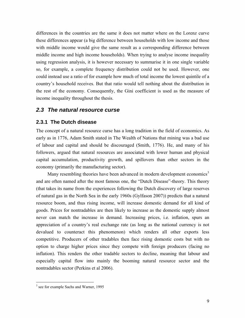
differences in the countries are the same it does not matter where on the Lorenz curve these differences appear (a big difference between households with low income and those with middle income would give the same result as a corresponding difference between middle income and high income households). When trying to analyse income inequality using regression analysis, it is however necessary to summarise it in one single variable so, for example, a complete frequency distribution could not be used. However, one could instead use a ratio of for example how much of total income the lowest quintile of a country’s household receives. But that ratio would tell nothing about the distribution in the rest of the economy. Consequently, the Gini coefficient is used as the measure of income inequality throughout the thesis.

2.3 The natural resource curse

2.3.1 The Dutch disease The concept of a natural resource curse has a long tradition in the field of economics. As early as in 1776, Adam Smith stated in The Wealth of Nations that mining was a bad use of labour and capital and should be discouraged (Smith, 1776). He, and many of his followers, argued that natural resources are associated with lower human and physical capital accumulation, productivity growth, and spillovers than other sectors in the economy (primarily the manufacturing sector).

Many resembling theories have been advanced in modern development economics3 and are often named after the most famous one, the “Dutch Disease”-theory. This theory (that takes its name from the experiences following the Dutch discovery of large reserves of natural gas in the North Sea in the early 1960s (Gylfason 2007)) predicts that a natural resource boom, and thus rising income, will increase domestic demand for all kind of goods. Prices for nontradables are then likely to increase as the domestic supply almost never can match the increase in demand. Increasing prices, i.e. inflation, spurs an appreciation of a country’s real exchange rate (as long as the national currency is not devalued to counteract this phenomenon) which renders all other exports less competitive. Producers of other tradables then face rising domestic costs but with no option to charge higher prices since they compete with foreign producers (facing no inflation). This renders the other tradable sectors to decline, meaning that labour and especially capital flow into mainly the booming natural resource sector and the nontradables sector (Perkins et al 2006).

3 see for example Sachs and Warner, 1995

9

The course of events described has theoretically two primary implications on economic growth. First, the decrease in production of tradables leads to a deviation from the country’s optimal development path which implies a lower growth rate. Second, a reduction of the traded sector means less learning by doing, since it is believed that it is primarily in the traded manufacturing industry that this positive externality appears. The result is a lower productivity growth than would otherwise be the case, reducing the growth rate even further. The combination of these two effects may eventually be sufficiently strong to outweigh the initial increase in income that the natural resource boom generated (Torvik 2009).

Apart from the Dutch disease-theory, two other categories of explanations to the natural resource curse appear frequently in the literature. These are discussed below.

2.3.2 Rent-seeking The role of rent-seeking has been proposed to explain the natural resource curse. By rent-seeking it is meant that instead of engaging in productive activities, people try to obtain a larger piece of the existing pie. For example, they may use bribes and other sorts of corruption to gain favourable treatment (such as special control rights, lower taxes etc) by the bureaucrats or the government (Perkins et al 2006). This distorts the economy in several ways, besides the obvious fact that labour and effort is used for non-productive activities, it may also result in non-optimal public policies and in non-optimal use of production factors (Bulte et al 2005). The negative effects of rent-seeking are thought to be extra severe when it comes to natural resources because the resource rents are easily appropriable. In natural resource abundant countries, such activities thus risk to reduce or even deprive the net gain of the natural resource (Torvik 2009).

2.3.3 Institutions and types of resources Second, a group of theories arguing that the resource curse operates through a combination of bad institutions and the type of resource has been put forward lately. It has been fairly proved that for example the level of corruption, rule of law and the risk of expropriation of private investment increase the risk of rent-seeking behaviour and conflicts which in turn have negative effects on economic development (Torvik 2009). The theories thus argue that there is no direct effect of resource abundance on economic performance but an important indirect effect if these institutions are of low quality. The windfall gains from natural resources give both rulers and other powerful people (such as oligarchs) higher than normal incentives to keep (or even create) bad institutions because

10

it allows them to ripe a bigger part of the gains themselves, at the cost of other parts of the society.

However, it is not only the quality of the institutions that matters but also the type of the natural resources. ‘‘Point resources’’, such as fuels and minerals, are, according to these theories, more likely to cause problems because the ownership and the gains could easily be concentrated in a few hands while food and agricultural raw materials, which are diffuse and less valuable natural resources, should have less or no effect (Bulte et al 2005 and Boschini et al 2007).

2.4 Implications on income inequality The natural resource curse theories outlined above have important implications for income inequality.

First, a natural resource boom should, according to the theory of “Dutch disease”, reduce the international competitiveness of the other sectors of the economy and, in turn, probably reduce the demand for labour in these sectors. Since many natural resources (most notably minerals and fuel) do not generate as much employment as other sectors (e.g. manufactures or small agriculture) the outcome is likely to be higher unemployment and/or lower equilibrium wage rate and rising return on capital. By the assumption that capital (and thus the return on capital) is controlled by a minority of the population, this reasoning gives that (even if the GDP/capita rises) income inequality should increase (Berry 2008 and Ross 2007). The reasoning hence supports an argument analogous with hypothesis 2, stated above.

Second, if natural resources give rise to rent seeking (as proposed by the second natural resource curse theory), it is highly probable that this in turn will lead to higher income inequality. In order to not do that the natural resource rents in fact need to be more equally distributed than labour income among the population. Since the very idea of rent-seeking is to favour yourself at the expense of others this is however not probable (Gylfason 2007). Would natural resource abundance even decrease institutional quality, income inequality would most certainly increase since worse and less reliable institutions probably also means that some will be favoured at the expense of others. From this second strand of the natural resource curse theory, hypothesis 1 is derived.

Third, the notion of “point resources” should have similar implications on income distribution as on economic growth. Hence, if the type of the resource matters, fuel, metals and other such precious and concentrated resources should follow the pattern described above and increase income inequality while agricultural raw materials and food should have less or no effect. This theory is tested with hypothesis 3.

11

2.5 Previous research As indicated in section 2.3, the research on the natural resource curse is massive but the specific relationship between natural resource abundance and income inequality has received much less attention. However, a few previous studies should be noted.

Most recently, Goderis and Malone conducted a study on natural resources and income inequality drawing on the same statement from Ross (2007) as is cited in the introduction of this thesis. Yet it differs in several aspects from the analysis carried out here. First of all, Goderis and Malone only investigate the effect of a change in natural resource abundance, neglecting the question of what a constant high or low level would imply. Second, they develop a formal theory in the context of a two sector growth model, predicting that income distribution would turn slightly more equal immediately after a natural resource boom but then slowly return to the initial distribution as the economy grows. Their panel data analysis of 90 countries between 1965 and 1999 strongly supports the theory. Hence, making no theoretical use of the natural resource curse they develop and find evidence for a reasoning that is contrary to mine (that an increase in natural resource abundance would imply a less equal income distribution and this effect is supposed to be stable until the resource abundance eventually declines).

A first glance at the results from the Goderis and Malone empirical analysis seems to increase the odds of my hypotheses but several aspects in their empirical testing change the picture. First of all they measure the difference in the Gini coefficient as annual changes although “income distribution statistics are not expected to change markedly between two successive years” (Odedokun and Round 2004, p292). Hence, much of the assessed changes could as well depend on measurement error as on actual changes. Second, their data on both income inequality and natural resources could be questioned. To measure income inequality they use a dataset from Galbraith and Kum (2005) with estimated measures of income inequality which gives a very comprehensive but not so reliable sample. What is even more disputable however, is their proxy for natural resources. Instead of measuring actual changes in a country’s resource dependency, they construct weights by dividing the individual 1990 export values for 50 different commodities by the total value of 1990 commodity exports for each country. These weights are then used for each year during the whole period and are only adjusted for the world price change in the commodities. Hence, when comparing a country’s, say, natural gas exports in 1965 and 1990 the weight is the same, no matter if the natural gas had been discovered or not in 1965.

12

Apart from Goderis and Malone, Berry (2008) concludes in a case study of four mineral dependent developing countries that the challenge to achieve good enough employment growth in order to avoid a high or rising level of inequality under mineral dependency is severe. Leamer et al (1999) also shows in a paper that since large natural resource sectors hinder capital to flow to the manufacturing sector, this depresses workers’ incentive to accumulate skills. Such a development could, they argue, explain a stable higher level of income inequality since the large income differences between the capital owners and the rest of the population is sustained. The conclusion is consistent with the theory of rent-seeking used in this thesis.

By relaxing the definition of natural resources one step, it could also be argued that Sokoloff and Engerman (2000) in their much cited work on factor endowments, institutions and income inequality study a similar topic. They explain the different development of income inequality in European colonies in the Americas by their initial endowments. In the southern colonies, the most profitable option was to produce cash crops with considerable economies of scale (such as sugar or cotton) while the northern were best suited to crops that required smallholder production, such as grain. This conditioned the early development of their institutions since cash crops favoured very unequal systems, with economic and political power concentrated in the hands of a few land owners whereas the absence of economies of scale led to a much more egalitarian land distribution. Sokoloff and Engerman argue that this initial difference explains why North America sustained institutions that emphasised equal opportunities while in South America the political institutions that favoured the rich and excluded the poor remained. Hence, even if their research differ in scope and time span, it still apply to the rent-seeking and institutional approach to the natural resource curse and its expected implications for income distribution.

2.6 What else determines income inequality? Of course, many other factors than natural resources probably affect a country’s income distribution. However, the literature on the determinants on income inequality is as dispersed as it is large. For a long time, Simon Kuznets’ notion of a quadratic relationship between economic development and income inequality was the prevailing main explanation. According to Kuznets (1955), higher and more dispersed returns of factors of production in industry compared to in agriculture implied that the least developed countries, where almost everyone were supposed to work in the rural sector, should be the most egalitarian. In countries that had commenced to industrialise, inequality should rise because of the different returns from the two sectors but when the transition from the

13

low-return rural to the high-return industrial sector was almost accomplished income inequality should start to fall again. This relationship, which should look like an inverted U, is commonly denoted the Kuznets curve and was until the late 1980s most often supported in empirical studies (Perkins et al 2006). However, more recent research has rejected this theory empirically by showing that such a pattern rather arises from country specific effects. Neither, a robust, strong case for a simple linear relationship exists (Deininger and Squire 1998). Nevertheless, empirical results supporting either the Kuznets curve (Thornton 2001), a positive linear trend (e.g. Odedokun and Round 2004) or a negative linear trend (Goderis and Malone 2008) are still not unusual.

Many other variables have been proposed to influence income distribution and quite a few of them have received at least some empirical support. Below, I mention some of the most convincing ones. For example, the inflation rate has been proved to have a decreasing impact due to the unexpected component (Mocan 1999 or Bishop et al 1994) while Li et al (2000) and Gyimah-Brempong and de Camacho (2006) among others reveal an increasing effect of the level of corruption. Goderis and Malone also find support for an equalising impact of democratisation.

A few variables have proven to be significant in many analyses but with different effects. These include government expenditures which theoretically have been thought to have a decreasing effect on income inequality but in empirical analyses, the results have been mixed (see for example Odedokun and Round 2004 and Tanninen 1999). That the level of trade openness should have some impact on the income distribution is also often supported but the sign of the coefficient differs. Barro (2000) finds it to increase income inequality while Milanovic (2005) says it mainly has a reducing effect.

14

3 Method and data

3.1 Method As stated in the introduction, this thesis uses a statistical approach in order to test the hypotheses put forward. Since the main purpose is to conclude if any general trends regarding natural resources and income inequality can be observed, a more qualitative approach, for example a comparative case study, would not have been to very much help. Instead, a dataset as large and as reliable as could be found was compiled, resulting in an unbalanced panel consisting of yearly data between 1962 and 2006 for a maximum of 101 countries.

The unbalancedness results from the fact that for many countries, there does not exist data for all variables during the entire period (this is especially the case for income inequality data). As long as full information for a country exists for at least two periods of study, it has nevertheless been included. Countries with only one observation were dropped since these could not be included in the regression models where country fixed effects were used (see section 3.1.3 for explanation). Hence, the actual number of included countries is 85 when regressing the level of income inequality on the level of natural resource dependency and 77 when testing for changes in the same variables.

The data (discussed in detail in section 3.2) has been processed and analysed in the statistical software package Stata (v10.0).

3.1.1 Control variables As stated in section 2.6, many studies of the determinants of income distribution have been conducted before and many variables have been claimed to have impact on income distribution. In order to control that natural resources have a specific effect on the Gini coefficient even when accounting for other possible explanatory variables some of these have been included in the regression analysis. These variables which already have been mentioned in section 2.6 are:

− GDP per capita − Squared GDP per capita (I chose to include also the squared term of the GDP per

capita in order to account for the Kuznets curve since it turned out to have at least as much explanatory power as only the linear term)

− Openness to trade − Level of democracy − Government expenditure

15

(Data sources of these variables are discussed in section 3.2.6) Some of the variables highlighted by other studies have not been included because of one of three reasons:

(i) they are believed to be an effect of the natural resource abundance/boom (e.g institutional measures and inflation rate). Including for example the inflation rate as an individual explanatory variable would not make sense since, according to the Dutch disease theory, a natural resource boom affects the inflation rate which I in turn suggest affects the income distribution.

(ii) they proved to be completely insignificant in any regression specification (iii) they reduced the number of observations dramatically.

However, some variables were used to test the robustness of the results and none of them altered the natural resource coefficients significantly.

3.1.2 Causality The problem of knowing which variable that is the causal one is a fundamental problem in many econometric studies. To try to correct for this problem, all independent variables in the regressions have been lagged compared to the independent ones. When lagging the independent variables, it should be impossible to have an inverse causality since the dependent observation not yet has taken place at the time of the independent observation.

However, if an observation is part of a trend spread out over several periods, this is no longer the case. Even if a correlation is found between the assumed dependent variable and the assumed lagged independent variable, the true causality could be the other way around, a long lasting trend in the “dependent” variable affects the lag in the “independent” one. Neither is it possible to be completely sure of the optimal lag. In this case, how many years does it take for natural resources to affect income distribution? A too short lag may mean that an actual correlation is missed because the effects take longer than the lag used. A too long lag could imply essentially the same thing, if a change in one variable affects another almost immediately, running a regression with a five year lag would miss the correlation completely. By logical reasoning when choosing different lags, I have tried to minimise the risks of inverted causality but the essential problem should nevertheless be kept in mind when looking at the final results.

16

3.1.3 Specification of the regression models To obtain the most accurate results in my empirical analysis, the data and the hypotheses have been tested using several different econometrical techniques. The four different models are described and motivated below.

To start with, all equations have been regressed as pooled cross sections by using a simple Ordinary Least Square (OLS) method.4 In this setting, the data is regarded to be cross-sectional and the fact that there exists more than one observation for many countries but originating from different time periods is ignored. Instead, each observation is practically regarded as a specific country, implying that when running the first regression in section 4.1 with 559 observations, this could be interpreted as comparing a sample of 559 different countries at the same time. This does not need to be problematic, as long as I could prove, or at least argue convincing, that the data does not exhibit unobserved time and/or country specific effects.

However, it seems very reasonable that there exist such effects which the OLS-model fails to take into account. First, it would be rather strange if a certain country would not have a wide range of specific features that are highly consistent over time. Such specific effects could be anything from “culture” to a constantly undervalued exchange rate which may or may not influence income distribution. It is exactly the fact that I cannot give a complete list of them that makes it impossible to incorporate these variables in a cross-sectional setting. To test if the data shows signs of time persistent country heterogeneity, I tested a null hypothesis saying that individual dummy variables for each country were jointly equal to zero against a two-sided alternative. This null hypothesis was rejected at a 1% significance level (F statistic) for all regression equations used to test the hypotheses, thus implying that the models should be corrected for unobserved country fixed effects.

A country fixed effects model was obtained by using the within regression estimator.5 This estimator time-demeans the dependent as well as all the independent variables and the error term which makes the unobserved fixed effect disappear from the equation. The time-demeaned variables are then regressed by pooled OLS (Wooldridge 2009). This is performed automatically by most statistical software packages (in this case Stata v10.0) which also reports the “eliminated intercept” but this is actually only the average of the automatically obtained individual-specific intercepts (Wooldridge 2009).

4 see for example Wooldridge 2009 5 See Wooldridge 2009 or Park 2009 for a thorough review of within estimation.

17

Since this model automatically corrects for all time-constant variables, no such variables could be included in the analysis.

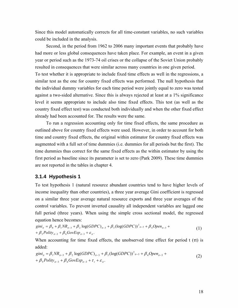
Second, in the period from 1962 to 2006 many important events that probably have had more or less global consequences have taken place. For example, an event in a given year or period such as the 1973-74 oil crises or the collapse of the Soviet Union probably resulted in consequences that were similar across many countries in one given period. To test whether it is appropriate to include fixed time effects as well in the regressions, a similar test as the one for country fixed effects was performed. The null hypothesis that the individual dummy variables for each time period were jointly equal to zero was tested against a two-sided alternative. Since this is always rejected at least at a 1% significance level it seems appropriate to include also time fixed effects. This test (as well as the country fixed effect test) was conducted both individually and when the other fixed effect already had been accounted for. The results were the same.

To run a regression accounting only for time fixed effects, the same procedure as outlined above for country fixed effects were used. However, in order to account for both time and country fixed effects, the original within estimator for country fixed effects was augmented with a full set of time dummies (i.e. dummies for all periods but the first). The time dummies thus correct for the same fixed effects as the within estimator by using the first period as baseline since its parameter is set to zero (Park 2009). These time dummies are not reported in the tables in chapter 4.

3.1.4 Hypothesis 1 To test hypothesis 1 (natural resource abundant countries tend to have higher levels of income inequality than other countries), a three year average Gini coefficient is regressed on a similar three year average natural resource exports and three year averages of the control variables. To prevent inverted causality all independent variables are lagged one full period (three years). When using the simple cross sectional model, the regressed equation hence becomes:

.))(log()log(

3635

3432

332310

ititit

ititititit

GovExpPolityOpenGDPCGDPCNRgini

εβββββββ

++++++++=

−−

−−−− (1)

When accounting for time fixed effects, the unobserved time effect for period t (τt) is added:

.))(log()log(

3635

3432

33231

ittitit

ititititit


ετββββββ

++++++++=

−−

−−−− (2)

18

When accounting for country fixed effect, an unobserved country fixed effect for country i (αi) is added instead:

itiitit

ititititit


εαββββββ

++++++++=

−−

−−−−

3635

3432

33231 ))(log()log( (3)

Finally, with a two-way fixed effect model, both effects are added:

itititit

ititititit


εατββββββ

+++++++++=

−−

−−−−

3635

3432

33231 ))(log()log( (4)

(since the last equation in fact is regressed with time dummy variables in Stata, τt is in reality a set of T-1 dummies with individual coefficients but the interpretation is the same). The variables are as follows: giniit = Gini coefficient for country i at time t NRit-3 = Natural resource exports for country i at time t-3 Log(GDPC)it-3 = GDP per capita for country i at time t-3 (logarithmic) Log(GDPC)2

it-3 = Squared GDP per capita for country i at time t-3 (logarithmic) Openit-3 = Openness to trade for country i at time t-3 Polityit-3 = Polity score for country i at time t-3 GovExpit-3 = Government expenditure for country i at time t-3

3.1.5 Hypothesis 2 To test hypothesis 2 (natural resource booms increase a country’s income inequality, and vice versa) I regress the changes over time in the two variables of interest. Further, I include the initial level of natural resource exports as well in order to be able to compare the effect of a change with the effect of a certain level of abundance.

In line with Odedokun and Round (2004) (quoted in section 2.5) I think that annual changes in the Gini coefficient (a rather stable variable that risks to be flawed with measurement errors) may depend on chance as well as on causal relationships and therefore I use three year intervals instead. All control variables used to test hypothesis 1 seems equally valid in this setting and are therefore included. However these are still three year averages since it is their relative levels that are believed to influence income inequality development. In addition to these control variables, the initial Gini coefficient is also added since it seems plausible that a very high (low) coefficient poses restrictions on future increases (decreases).

A potential problem when using individual natural resource observations or when calculating the difference between two of them is that large annual price fluctuations in some resources could have adverse effects on the result. To counteract this problem, each

19

“yearly” observation was calculated as a mean of the actual year, the preceding year and the following year. Hence, when computing the change in primary exports 2001-2004, “year 2004” was the average of the years 2003, 2004 and 2005 and “year 2001” was the average of the years 2000, 2001 and 2002. Even if the same problem does not arise for the Gini coefficient, this was calculated in the same way for reasons of comparability.

In order to prevent inverted causality all independent variables are lagged one year, meaning that change in natural resource exports 2001-2004 is compared with a change in the Gini coefficient 2002-2005.A full period lag (i.e. three years) was considered but deemed inappropriate since an eventual effect of natural resources should be fairly immediate. The four regression equations used in the second analysis are thus: Simple cross-sectional OLS:

itititit

itititititit

GovExpPolityOpenGDPCGDPCNRNRGinigini

εβββββββββ

+++++++Δ+++=Δ

−−−

−−−−−

181716

12

5141342310 ))(log()log( (5)

Time fixed effects:

ittititit

itititititit


ετββββββββ

++++++++Δ++=Δ

−−−

−−−−−

181716

12

514134231 ))(log()log( (6)

Country fixed effects:

itiititit

itititititit


εαββββββββ

++++++++Δ++=Δ

−−−

−−−−−

181716

12

514134231 ))(log()log( (7)

Time and country fixed effects:

ititititit

itititititit


εατββββββββ

+++++++++Δ++=Δ

−−−

−−−−−

181716

12

514134231 ))(log()log( (8)

(since the last equation in fact is regressed with time dummy variables in Stata, τt is in reality a set of T-1 dummies with individual coefficients but the interpretation is the same). The variables are as follows: Δginiit = Change in the Gini coefficient for country i during time t giniit-3 = Gini coefficient for country i at time t-3 NRit-4 = Natural resource exports for country i at time t-4 ΔNRit-1 = Change in natural resource exports for country i at time t-1 Log(GDPC)it-1 = GDP per capita for country i at time t-1 (logarithmic) Log(GDPC)2

it-1 = Squared GDP per capita for country i at time t-1 (logarithmic) Openit-1 = Openness to trade for country i at time t-1 Polityit-1 = Polity score for country i at time t-1 GovExpit-1 = Government expenditure for country i at time t-1

20

3.1.6 Hypothesis 3 To test the third hypothesis (if there exists a relationship between natural resources and income inequality this depends on the type of resource), an augmented version of those models used to test hypothesis 1 and 2 is used. But, instead of using the complete primary exports variable (which include both “point resources” such as ores and oil, and other exports such as rice or meat), I include three mutually excluding subsections: (i) agricultural raw materials and food exports, (ii) fuel exports, and (iii) ores and metals exports. The eventual different effects of these three components are then evaluated in order to reach a conclusion.

The subsections follow the definitions used by the United Nations Conference on Trade and Development (UNCTAD)6 and were chosen to in a simple way discern different kind of resources. For example, agricultural raw materials and food exports effectively distinguish cultivable resources from “existing” ones. The division of the non-renewable resources in ores and metals on the one hand and fuels on the other is maybe a little bit more far-fetched. However, the reason is that fuels several times have been pointed out to be quite a special case. First, no other natural resource is even close to have such a great influence on a country’s economy, especially in the Middle East. Second, more often than is the case for other natural resources, fuel reserves are controlled or even owned by the government which implies that the consequences for income distribution could be different than for privately owned resources. For example, both inflation and rent-seeking could be suppressed by the government if they responsibly take care of the gains. Ross (2007) also demonstrates that oil exporting countries have considerably larger public sectors than similar countries and according to Milanovic (2001), governments tend to compress the wages of their employees which should have an equalising effect on income distribution.

3.1.7 Sensitivity analysis and robustness tests To control the robustness of the empirical results, a few measures are taken. First of all, all regression models was tested for, and showed strong signs of, heteroskedasticity. The null hypothesis that the error term was homoskedastic was always rejected also at a 1 % significance level. As a consequence, the regression results reported in this thesis have all been obtained by using White’s heteroskedasticity-robust standard errors. Second, the regression models as well as the data were modified in several ways in order to test if this

6 see for example UNCTAD Handbook of Statistics 2008 for a complete definition on each category

21

altered the result. The tests and their results could not be included explicitly in the thesis but the tests are described and important findings are reported in section 4.3.

3.2 Data In this section, all data used in the empirical analysis is presented and discussed. Descriptive statistics of each variable are presented in table 3.1.

3.2.1 General comments on the data sample Completely depending on secondary data, the empirical analysis is subject to several potential problems. First, it is beyond my capacity to control the validity of each observation. The data could thus suffer both from mere typing errors and from measurement errors arisen when collecting the primary data. The first problem could be somewhat controlled for by analysing the descriptive statistics of all variables in table 3.1. Apart from concluding that the summarised observations seem reasonable not much could be done even if the robustness test (reported in section 4.3) where outliers are excluded could control for flagrant typing errors. Similarly, the risk of measurement errors could be noted but not really corrected for. For this reason, the statistical sources used have been chosen with the twofold objective of both generate a large enough sample and have a high degree of reliability. Table 3.1 Descriptive statistics Observations Mean Standard

deviation. Minimum value Maximum value

Gini (average) 559 46.5091 7.4889 27.2275 78.6050

Primary exports (average) 559 0.1000 0.0826 0.0022 0.6762 Agricultural raw materials and food exports (average) 559 0.0593 0.0558 0.0009 0.3310

Fuel exports (average) 559 0.0270 0.0622 0 0.6500

Ores and metal exports (average) 559 0.0137 0.0303 0 0.4257

Per capita income (average) 559 8136.9210 8794.4270 131.6955 37964.8500

Openness to trade (average) 559 0.6108 0.3200 0.0975 2.0424

Polity score (average) 559 0.7548 0.3170 0 1

Government expenditure (average) 559 0.1990 0.0717 0.0710 0.5876

Gini (change) 489 0.1173 2.6890 -12.0623 8.6958

Primary exports (change) 489 -0.0034 0.0254 -0.2730 0.1001 Agricultural raw materials and food exports (change) 489 -0.0030 0.0143 -0.0581 0.0662

Fuel exports (change) 489 0.0002 0.0187 -0.2665 0.0867

Ores and metal exports (change) 489 -0.0005 0.0070 -0.0814 0.0422

22

3.2.2 Time span In the empirical analysis, data for the period 1962-2005 have been used. The period was chosen in order to construct a data set containing as many observations as possible from the chosen sources. Since natural resource data was not obtainable for years preceding 1962 this was chosen as the base year. In a similar manner, 2005 was chosen as the end year since it was not possible to obtain observations for all variables for years thereafter. As a standard, three year periods have been analysed since annual periods were deemed unreliable and longer periods resulted in too many lost observations. Because of the use of lagged and three year mean variables described in section 3.1.4 and 3.1.5 the maximum number of analysed periods was 13 (starting in 2005 and backwards) when testing levels as well as changes.

3.2.3 Included countries In appendix A, a full list of included countries along with the number of observed time periods for each of the two settings can be found. The sample comprises countries from all continents and with different levels of development but with a slight bias towards more developed countries. Obviously, this is a consequence of the fact that many developing countries lack complete data. In general, all countries with enough data are included in the analysis with two exceptions. These two are Belgium and Singapore which hardly have any natural resources but nevertheless show up as big primary exporters in the data. This is due to the fact that they import large quantities of natural resources and then re-exports them without processing them enough to re-label them to manufactured products. Because of this inconsistency these countries are excluded.

3.2.4 Income inequality A great drawback on the comparability of income inequality data is the multitude of different techniques and definitions used when collecting it. To start with, it is not always income distribution that is measured but instead consumption or wealth distribution. Any of these distributions could also be reported as either per household, per employee or per person, and on top of that the distribution could be reported as either net or gross income. Apparently, such differences greatly impair the comparability of different data sources and are the main explication of the unreliability of many empirical studies of income inequality. Often, researchers have had to choose either to only use fully comparable data and end up with a very small dataset or to ignore the problem and use different measures anyway.

23

To bring order to the field of income distribution, Deininger and Squire assembled in 1996 the to that date biggest compilation of economic inequality data by combining earlier datasets that were deemed to live up to a certain quality but still was not completely comparable. Even though they clearly stated the comparability problem, the full set has been used in hundreds of cross-national studies, usually with low or no precaution. This compilation has today evolved to the World Income Inequality Database (WIID), provided by the World Institute for Development Economics Research of the U.N. University and contains over 5000 observations in 160 different countries. However, the main problem of incomparable observations remains, implying that the most comprehensive set of truly comparable observations only includes 508 observations in 71 countries.

To resolve this problem, however, Solt (2009) recently has tried to format all observations in the WIID to one single income distribution measure by using a custom missing-data algorithm and another smaller but highly reliable data set (the Luxembourg Income Study) as a standard.7 The result was a set of 3331 observations of net income inequality and 3273 of gross income inequality, called the Standardized World Income Inequality Database (SWIID). To date, this is the largest and most reliable database existing, which therefore is used in the analysis.

In the choice between using net or gross income observations, I have chosen to use the latter. This is because the study aims to see what the effect of natural resources has on income distribution, ceteris paribus. If natural resource dependency at first affects income distribution but then is differenced away by progressive redistributive policies, we will have two effects that are equally important but together equals out their respective effects. To avoid such a situation, the gross income seems to be the only correct measure. Using net instead of gross figures makes a great difference in highly redistributive countries as Sweden but in most other countries, especially developing countries, the difference is not that big since they have quite uniform taxes and limited redistributive powers (Solt 2009).

3.2.5 Natural resource exports The four different measures of natural resources all come from the World Bank’s World Development Indicators (WDI) database. The WDI however reports these statistics as share of merchandise exports whereas the natural resource curse literature primarily uses exports as share of GDP (for reasons described in section 2.1). Therefore the observations

7 for a thorough explanation of how the standardisation was carried out, see Solt 2009

24

had to be rescaled by using the WDI statistic of total merchandise exports which in turn could be divided with its statistic for annual GDP. Although requiring a little calculation, such rescaling should not have any negative effect when it comes to reliability.

3.2.6 Control variables Reliability does not only depend on how carefully a single observation is collected, but also on how it was processed compared to another observation. Different data providers often use slightly different processing or calculation techniques which could have different effects on the final value. To get a correct relation between the natural resources variables and the control variables (as well as between the control variables) the latter were, as far as possible, taken from the same data provider as the natural resource statistics, the WDI. Below is a short description of the data and its source for each variable.8

Per capita income – To measure per capita income, and thus the level of economic development attained I used WDI:s indicator for GDP/capita in constant prices. Constant prices were chosen to keep inflation out of the picture.

Openness to trade – To account for a country’s openness to trade, WDI:s measure of trade as a percentage of GDP was used. Other proxies (such as changes in tariff revenues) were considered but this was chosen because of its common use and high data availability.

Government expenditure – To measure government expenditure I used the Penn World Table (PWT) Mark 6.2 indicator of “Government share of real GDP in constant prices”. The WDI database also include an expenditure statistic but since this is not completely inclusive, I deemed the PWT variable to be more accurate even though yet another data provider had to be included.

Level of democracy – To account for how democratic a country is, I used the overall Polity measure from the Polity IV Project, a score that in my data is ranging from 0 to 1. 0 representing a completely autocratic regime and 1 representing a completely democratic one.

8 for more information about these variables, please see WDI (2009b), Heston et al (2006) and Marshall and Jaggers (2009)

25

4 Results In the following two sections, the main results of the empirical analysis are reported and commented. In 4.1, the hypothesis that natural resource abundant countries have higher income inequality (hypothesis 1) is tested and in 4.2 the hypothesis that an increase in natural resource dependency raises income inequality and vice versa (hypothesis 2) is tested. As mentioned above, the third hypothesis about the importance of different natural resources is tested simultaneously in both 4.1 and 4.2. In section 4.3, finally, the findings in the two first sections are tested for robustness.

4.1 Levels of income inequality Before running the first regression measuring the level of income distribution, the simple correlations between all variables used in these regressions are inspected. Table 4.1 reports these correlations and from the table, it can be seen that the Gini coefficient is mostly correlated with income per capita but that it is still on a very modest level. Regarding the measures of natural resources, the difference in their correlation with the Gini coefficient and the large spread of their intracorrelation are highly noteworthy. This implies that using different measures should give differing results and justifies the use of four different measures in the analysis.

The fairly large correlation difference between per capita income and the two first natural resource measures on the one hand and per capita income and the two last natural resources on the other could also be noted. A similar pattern is present for the openness to trade.

Table 4.1 Correlation matrix Gini Primary

exports Agr. and food exp.

Fuel exports

Ores and met. exp.

Per cap. income

(Per cap. income)2

Open-ness

Polity score

Gov. expend.

Gini 1.0000

Primary exports 0.1414 1.0000 Agricultural raw materials and food exports 0.2230 0.5631 1.0000

Fuel exports -0.0941 0.6639 -0.1259 1.0000

Ores and metals exports 0.1683 0.3261 -0.0464 -0.0126 1.0000

Per capita income (logarithm) -0.2720 -0.2542 -0.2772 -0.0461 -0.0882 1.0000 (Per capita income)2 (logarithm) -0.2849 -0.2675 -0.2842 -0.0525 -0.0984 0.9958 1.0000

Openness to trade -0.0538 0.3583 0.3582 0.1022 0.1077 0.0152 -0.0042 1.0000

Polity score -0.0778 -0.1134 -0.0089 -0.0735 -0.1420 0.6404 0.6390 0.1250 1.0000

Government expenditure -0.0697 0.1162 0.0770 -0.0011 0.1772 -0.1268 -0.1398 0.3129 -0.0367 1.0000

26

Inspecting only the control variables, it could be concluded that they all seem to be rather uncorrelated with each other except for income per capita and the polity score. This last correlation should however not be high enough to pose any statistical problems for the regressions. Lastly, it could be noted that the per capita income and the per capita income squared are, as they should be, almost completely correlated.

Next, we turn to the results of the regressions specified in section 3.1.4. Each table include the four different models used.

4.1.1 Primary exports In table 4.2, the broadest natural resource measure, primary exports, have been regressed by equations 1-4. Starting with the first column, reporting the simple cross-sectional regression, all control variables turn out to be significant at least on the 10% level. However the signs of the coefficients are ambiguous. The support for the Kuznets curve is indeed substantial with the linear per capita income term being positive and the quadratic term being negative, and also the openness trade have the expected negative sign. But the polity score have positive instead of the expected negative sign. Also the government expenditure coefficient has the intuitively wrong sign but this is in line with earlier results from Odedokun and Round (2004). When it comes to the variable of principal interest, the primary exports, it turns out to have a positive and significant impact on the Gini coefficient, thus an increase in a country’s share of primary exports would raise the country’s income inequality, as suggested by hypothesis 1. Table 4.2 Primary exports (1) (2) (3) (4)

22.6985** 21.5081* 52.2569** 43.1384* Intercept (11.4252) (11.5129) (21.5290) (22.0017) 7.9689* 8.5679* -1.9434 5.6660 Primary exports (4.4468) (4.5564) (4.2239) (4.5158) 8.3796*** 8.6937*** -5.7455 -0.5860 Per capita income (logarithm) (2.8509) (2.8728) (5.0263) (5.2671) -0.6514*** -0.6636*** 0.5830** 0.0884 (Per capita income)2 (logarithm) (0.1763) (0.1772) (0.2972) (0.3299) -2.4711** -3.2274*** -4.0288*** -5.1675*** Openness to trade (1.1419) (1.2446) (1.4051) (1.3599) 4.4866*** 4.2110*** 1.3667 -1.1560 Polity score (1.4105) (1.4720) (1.1081) (1.1379) -12.0695 -11.7397*** 12.7073* 16.0453** Government expenditure (4.2277) (4.3033) (6.5740) (7.0856)

Country fixed effects No No Yes Yes Time fixed effects No Yes No Yes R2 0.1439 0.1430 0.0702 0.1508 Countries 85 85 85 85 N 559 559 559 559 Notes: Dependent variable is Gini. Robust standard errors in parentheses. * Significant at 10%; ** significant at 5%; *** significant at 1%.

27

Turning to column 2, it shows that introducing time fixed effects does not alter the picture. The controls keep their signs and significance as well as primary exports.

When using country fixed effects instead though, the picture changes in several aspects. First, primary exports turn negative but it is far from significant. Also, the Kuznets curve is completely reversed, implying that an increase in an already high per capita income actually would raise income inequality but only one of the two terms is significant. The government expenditure follows the same trend and change sign while the polity score turns insignificant.

When combining the two fixed effects in column 4 the pattern of less significant variables from column 3 is firm. Not surprisingly, both per capita income terms turn insignificant, since they apparently inherit very different time and country fixed effects, but the inverted Kuznets curve remains. Notably, openness to trade continues to be significant at a 1% level and its impact is perceptible but not substantial. A 10 percentage points higher trade as a share of GDP would imply a half a point higher Gini coefficient. The variable of main interest, primary exports, regains its expected positive sign but is still insignificant. The polity score also reverses and take on the expected negative sign but remains insignificant.

Looking at the results from all four regression models, a conclusion, which will prove to hold for all forthcoming regressions as well, is that models that do not control for omitted fixed effects variables are biased. This is in line with the results of the income inequality article by Gourdon et al (2008) where the same conclusion is drawn. When comparing column 1 and column 4 directly, we can see that four out of six coefficients in fact have switched signs and only two remains significant

Regarding the results for primary exports, they give some but very limited support to hypothesis 1 since the variable is completely insignificant in the most accurate model. In line with hypothesis 3, I therefore continue the analysis by splitting primary exports in its three main parts, agricultural and food products, fuel, and ores and metals.

4.1.2 Subcategories Table 4.3 reports the results of similar regressions as those in table 4.2 but with the primary exports variable divided into three subsections, agricultural raw materials and food exports, fuel exports and ores and metals exports. A quick glance at the control variables, tells that these exhibit the same pattern in all four models as when using only primary exports. They are all significant at virtually the same levels and have the same signs.

28

The more interesting are the new natural resource variables. Beginning with column 1, all three categories seem to have significant but very different effects on the Gini coefficient. As supposed by hypothesis 1 and 3, ores and metals turn out to have a very large increasing effect, significant at the 1% level but the other variables rather oppose hypothesis 3. Agricultural and food products have also a significant and positive (but smaller) effect while fuel, which is as much a “point resource” as ores and metals, actually seems to have an equalising effect on the income distribution. Table 4.3 Subcategories (1) (2) (3) (4)

22.7423** 20.6542** 62.3737*** 54.0259** Intercept (10.4924) (10.4170) (21.9385) (21.9578) 23.7091*** 27.0243*** -19.5184** -8.5067 Agricultural raw materials and food

exports (6.5960) (6.9318) (8.7338) (8.8580) -8.4338** -8.3611*** -2.6827 2.9021 Fuel exports (3.3558) (3.5929) (4.7651) (4.4067) 46.9647*** 48.6960*** 46.7131*** 58.8913*** Ores and metals exports (6.3547) (6.5590) (14.0789) (14.0462) 8.1246*** 8.6923*** -7.7265 -2.3785 Per capita income (logarithm) (2.6535) (2.6329) (5.1312) (5.3070) -0.6203*** -0.6415*** 0.6840** 0.1548 (Per capita income)2 (logarithm) (0.1656) (0.1643) (0.3038) 0.3334 -3.3218*** -4.5539*** -4.1763*** -5.3120*** Openness to trade (1.1998) (1.3310) (1.4238) (1.3586) 4.1919*** 3.4180** 1.4074 -1.2046 Polity score (1.4625) (1.5669) (1.0987) (1.1249) -14.0619*** -14.0064*** 10.6366 12.7602* Government expenditure (3.9229) (4.0081) (6.5079) (7.0045)

Country fixed effects No No Yes Yes Time fixed effects No Yes No Yes R2 0.1998 0.2045 0.0932 0.1738 Countries 85 85 85 85 N 559 559 559 559 Notes: Dependent variable is Gini. Robust standard errors in parentheses. * Significant at 10%; ** significant at 5%; *** significant at 1%. To control the validity of these findings, we turn to more specified regressions in columns 2 to 4. First, adding time fixed effects to the data does not alter the picture at all but rather confirms and amplifies the same results. When controlling for country fixed effects however, several changes occur. The effect of agricultural raw materials and food is completely reversed and now seems to have a significant and almost as large negative effect as its positive one in the first model. A similar but not as strong trend can be noted for fuel. Its negative effect is reduced by two thirds and is insignificant even at the 10 % level. When it comes to the last measure, ores and metals, the effect is stable: the sign, size and significance all remain the same as in previous models.

By controlling for both time and country fixed effects in column 4 it can be concluded that unobserved country fixed effects have a great impact on income

29

distribution since the trend from column 3 to a large extent persists. Not surprisingly though, the agriculture term turns insignificant since country and time specific effects apparently have very different consequences. Since it remains negative it indicates that the latter is more important but not enough to make it statistically significant.

With the two-way fixed effects model, fuel enters for the first time with the expected positive sign but not surprisingly it is completely insignificant, hence implying that fuel abundance have no or very different effects on income distribution. This is an obvious setback to hypothesis 1 and 3 since fuel is a “point resource” that should have an increasing effect on income inequality.

When moving on to ores and metals, the supportive trend from the previous columns is even amplified. As the only significant natural resource variable in column 4, it turns out to have a clear positive effect on income inequality. The coefficient takes on such a high value in the fourth regression that merely a 1.7 percentage point higher export of ores and metals as share of GDP would, ceteris paribus, entail a 1 point higher Gini coefficient. The result clearly supports hypothesis 1 and when contrasted to agricultural raw materials and food also hypothesis 3. However, the case of fuel blurs the picture.

Briefly comparing column 4 in table 4.2 and 4.3 supports this conclusion, since it proves that it is ores and metals that drive the positive result of primary exports. With these encouraging findings, we move on to see if a similar relationship can be traced also in actual changes in income inequality.

4.2 Changes in income inequality As in the previous section, I begin by investigating the correlations between the regressed variables. The five last control variables are the same as in section 4.1 and hence, their intracorrelations are similar. However, the initial value of the Gini coefficient is also included in the model and appears to have a negative correlation with a change in the Gini coefficient. When looking at the eight natural resource variables, it can be noted that the initial levels of natural resource dependency are higher correlated with the Gini change than the changes in resource dependency. We will see if this holds in the regressions as well.

It could also be noted that changes in all four natural resource variables are quite highly negatively correlated with the initial dependency. Lastly, we see that all of the control variables have very modest correlations with both the dependent variable as well as with the natural resource variables.

30

Table 4.4 Correlation matrix

Gini (change)

Gini (value)

Prim. exp. (share)

Agr. food exp. (sh.)

Fuel exp. (share)

Ores met. exp. (sh.)

Prim. exp. (change)

Agr. food exp. (ch.)

Fuel exp. (change)

Ores met. exp. (ch.)

Per capita income

(Per cap. income)2

Openness to trade

Polity score

Gov. expend.

Gini (chan ge) 01.0 00

Gini (initial va lue) 6 0-0.2 30 1.0 00

Primary exports (initial share) -0.0992 0.1933 1.0000

Agricultural raw materials and food exports (initial share) -0.0835 0.2410 0.6461 1.0000

Fuel exports (initial share) -0.0202 -0.0646 0.6220 -0.0915 1.0000

Ores and metals exports (initial share) -0.0738 0.1896 0.3028 -0.0342 -0.0165 1.0000

Primary exports (change) -0.0315 -0.0487 -0.4191 -0.1861 -0.3644 -0.0949 1.0000

Agricultural raw materials and food exports (change) 0.0063 -0.0719 -0.2690 -0.3620 -0.0229 0.0235 0.6177 1.0000

Fuel exports (change) -0.0677 0.0386 -0.2863 0.0334 -0.4725 0.0512 0.7459 0.0128 1.0000

Ores and metals exports (change) 0.0541 -0.1332 -0.2058 -0.0249 -0.0120 -0.5299 0.3728 0.1646 0.0068 1.0000

Per capita income (logarithm) 0.1128 -0.3053 -0.2425 -0.3013 0.0021 -0.0787 0.1126 0.1269 0.0308 0.0670 1.0000

(Per capita income)2 (logarithm) 0.1100 -0.3191 -0.2583 -0.3086 -0.0082 -0.0888 0.1146 0.1263 0.0340 0.0672 0.9957 1.0000

Openness to trade -0.0242 -0.0179 0.3708 0.3808 0.0916 0.0962 -0.1172 -0.1748 -0.0033 -0.0594 -0.0052 -0.0263 1.0000

Polity score 0.0932 -0.1001 -0.0688 -0.0046 -0.0335 -0.1246 0.0310 -0.0069 0.0325 0.0398 0.6368 0.6357 0.1050 1.0000

Government expenditure 0.1094 -0.0553 0.1133 0.1248 -0.0504 0.1716 -0.0182 -0.0410 -0.0000 0.0180 -0.1017 -0.1160 0.2908 -0.0249 1.0000

4.2.1 Primary exports As in section 4.1, I start by regressing equation 5-8 on the broadest natural resource measure, primary exports. The results are presented in table 4.5.

Looking at the control variables, the most noteworthy is that the initial value of the Gini coefficient has a very significant and increasing effect on the future development of the Gini coefficient all through the four regression models. That is, a higher initial Gini coefficient results in a lower change than otherwise (whether the predicted change itself is positive or negative of course depends on all variables). One possible interpretation of this is that income distribution, in itself is a converging force. For a country with a high Gini coefficient, it is more probable that it will decrease no matter what the other variables look like but for a country with a really low initial Gini coefficient, the risk that other factors will increase the Gini coefficient is higher.

The other controls, included as average values exactly as in section 4.1, show a similar but less significant pattern as when studying levels. Focusing on the fourth and most accurate regression, the trade openness, polity score and government expenditure variables all have the same signs and significance levels. When it comes to the per capita income terms, these now have “Kuznets-supporting” coefficients also with the two-way fixed effects model but since they are not close to be significant, it is of minor importance.

Turning to the natural resource variables, we can tell that in column 1, which reports the simple cross-sectional regression, hypothesis 2 is completely rejected. The initial share of primary exports as well as its change during the period has significant negative effects on the Gini coefficient. The result hence implies that both a high initial resource dependency as well as an increase in resource dependency would decrease income inequality. Adding time and country fixed effects somewhat alters this picture (especially when using the two-way fixed effects model) but at the same time, both terms turn completely insignificant. The sole conclusion to draw is thus that primary exports dependency does not affect the development of the Gini coefficient and nor does primary exports booms. By splitting the measure in three, we will try to determine if this is because of opposing effects by different resources or if it is because no relationship exists.

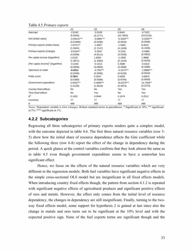
Table 4.5 Primary exports (1) (2) (3) (4)

-2.6162 -3.0109 6.6441 -0.7622 Intercept (5.5044) (5.2777) (22.7663) (23.5118) -0.09151*** -0.0881*** -0.3320*** -0.3325*** Gini (initial value) (0.01906) (0.0186) (0.0534) (0.0568) -2.8721** -1.6507 -1.5681 6.0524 Primary exports (initial share) (1.5924) (1.7147) (4.1249) (5.1535) -8.9164** -5.3547 -5.2191 -0.4996 Primary exports (change) (4.6269) (4.8111) (5.5428) (6.0052) 1.6125 1.6691 -1.4300 1.9868 Per capita income (logarithm) (1.3871) (1.3360) (5.1224) (5.4529) -0.1034 -0.1013 0.2688 -0.0315 (Per capita income)2 (logarithm) (0.0839) (0.0805) (0.2908) (0.3280) -0.5311 -0.7557** -3.1574*** -2.8985*** Openness to trade (0.3269) (0.3595) (0.9139) (0.9503) 0.7814 0.3547 0.5406 -0.8876 Polity score (0.5369) (0.5589) (0.8794) (0.9009) 4.5423*** 4.4085*** 16.6373*** 14.7350** Government expenditure (1.6135) (1.6616) (5.4970) (6.2270)

Country fixed effects No No Yes Yes Time fixed effects No Yes No Yes R2 0.1002 0.0940 0.1974 0.2512 Countries 77 77 77 77 N 489 489 489 489 Notes: Dependent variable is Gini (change). Robust standard errors in parentheses. * Significant at 10%; ** significant at 5%; *** significant at 1%.

4.2.2 Subcategories Regressing all three subcategories of primary exports renders quite a complex model, with the outcome depicted in table 4.6. The first three natural resource variables (row 3-5) show how the initial share of resource dependence affects the Gini coefficient while the following three (row 6-8) report the effect of the change in dependency during the period. A quick glance at the control variables confirms that they look almost the same as in table 4.5 even though government expenditure seems to have a somewhat less significant effect.

Hence, we focus on the effects of the natural resource variables which are very different in the regression models. Both fuel variables have significant negative effects in the simple cross-sectional OLS model but are insignificant in all fixed effects models. When introducing country fixed effects though, the pattern from section 4.1.2 is repeated with significant negative effects of agricultural products and significant positive effects of ores and metals. However, the effect only comes from the initial level of resource dependency, the changes in dependency are still insignificant. Finally, turning to the two-way fixed effects model, some support for hypothesis 2 is gained at last since also the change in metals and ores turns out to be significant at the 10% level and with the expected positive sign. None of the fuel exports terms are significant though and the

33

change variable even has a negative instead of a positive sign, completely opposing its expected unequalising influence as a “point resource”.

The results reported in tables 4.5 and 4.6 could be summarised as ambiguous but with some support for hypothesis 2. Primary exports as such do not seem to have any influence on the changes in the Gini coefficient while one of two “point resource” categories does. The significance is however far less solid in this setting than when looking at changes. It is also clear that the initial share of resource dependency is more important than is an eventual boom or fall.

Table 4.6 Subcategories (1) (2) (3) (4)

-2.7252 -3.2566 18.5791 10.3769 Intercept (5.5852) (5.3811) (21.84579 (23.0092) -0.0912*** -0.0890*** -0.3433*** -0.3468*** Gini (initial value) (0.0193) (0.0187) (0.0538) (0.0583) -1.7110 -0.0081 -17.2811** -5.7508 Agricultural raw materials and food

exports (initial share) (2.3450) (2.4862) (7.4303) (8.0486) -3.7603* -2.7748 -2.3686 3.0522 Fuel exports (initial share) (2.1646) (2.1910) (5.0909) (5.8938) -3.5035 -2.3499 36.8875*** 50.1898*** Ores and metal exports (initial share) (6.0916) (6.5822) (10.9409) (13.1083) -5.6489 -4.1695 -11.0708 -9.8585 Agricultural raw materials and food

exports (change) (7.6851) (7.8802) (9.3439) (9.4184) -13.1300** -8.6335 -7.4298 -2.9411 Fuel exports (change) (6.4199) (6.5235) (7.4075) (8.0131) -1.2449 2.4482 15.7760 36.2279* Ores and metal exports (change) (15.0915) (18.1294) (19.3784) (24.0505) 1.6272 1.7300 -3.5801 0.3086 Per capita income (logarithm) (1.4017) (1.3536) (4.9474) (5.3866) -0.1033 -0.1033 0.3768 0.0299 (Per capita income)2 (logarithm) (0.0844) (0.0810) (0.2840) (0.3275) -0.5479 -0.8285** -3.4693*** -3.1927*** Openness to trade (0.3351) (0.3742) (0.9511) (0.9724) 0.7273 0.2535 0.6856 -0.8621 Polity score (0.5687) (0.5940) (0.8714) (0.9041) 4.4913*** 4.3469** 13.2941** 10.7179* Government expenditure (1.7389) (1.7845) (5.3642) (6.0864)

Country fixed effects No No Yes Yes Time fixed effects No Yes No Yes R2 0.1022 0.0963 0.2164 0.2700 Countries 77 77 77 77 N 489 489 489 489 Notes: Dependent variable is Gini (change). Robust standard errors in parentheses. * Significant at 10%; ** significant at 5%; *** significant at 1%.

4.3 Robustness tests To control the robustness of the results above, a few measures were taken. First of all, as mentioned above, all models have been regressed and reported with White’s heteroskedastic robust standard errors since all regressions appeared to have high risk of heteroskedasticity.

34

Furthermore, the models were regressed with a large amount of other variables that either have been shown to have significant effect in former studies or easily could be argued to have, no one altering the result of the variables of interest (i.e. the measures of natural resources) significantly.9

Most of these were completely insignificant but it can be noted that for example the level of investment as share of GDP (source: Penn Word Tables, Mark 6.2) seemed to have an increasing effect on both levels of and changes in income inequality at the 10 % significance level. Further, the ICRG (International Country Risk Guide) index of law and order had an equally significant but negative effect on the level of the Gini coefficient and their index of socioeconomic conditions seemed to have an as significant positive effect on the change in the Gini coefficient. However the ICRG variables were not included in the main specifications since they did not have enough observations.

It could also be noted that the models were regressed without the quadratic term of the level of income per capita to account only for linear relationships, resulting in that the linear term either was insignificant or had the same sign as the linear term in the main regressions. Also, the other controls were dropped one by one to see if this changed the impact of the natural resources but this was never the case. The value of the coefficient differed a little but no change of sign or significance level occurred.

As a third measure to test the robustness of the results, the data was cleared for

outliers using the DFITS command in Stata. Belsley et al (1980) suggest that all

observations with a DFITS-value larger than nk*2 (where k is the number of

independent variables and n is the number of observations) may be potential outliers and

these were therefore dropped from the dataset (35 of 559 observations when testing the

level of income inequality and 31 of 489 when testing the change in income inequality).10

Then, all equations were regressed again, confirming the natural resource results.

However, a few changes in the control variables were noted, particularly, the level of

government expenditure turned insignificant in the models testing hypothesis 1.

Lastly the original variables were regressed with different time periods and lags. As discussed earlier, the regressions risk suffering from inverted causality and it is not

9 These variables were: other GDP/capita variables, Penn World Table’s variable for trade openness, capital formation as share of GDP, investment share of GDP, domestic price level, population, average years of schooling and several of ICRG:s country risk variables. The results from all regressions are available from the author on request. 10 Countries with excluded observations are marked with asterisks in Appendix A.

35

possible to theoretically determine how long it takes for an independent variable to affect the dependent one. Hypothesis 1 was therefore tested with time periods of 5 and 10 years instead of 3 (and hence with lags of 5 and 10 years on the independent variables), resulting in similar or slightly stronger results but with much less observations and included countries. Not only because of the fewer periods but also because many countries had missing data for a year or two in these 5 or 10 year periods which disqualified them from the sample.

When testing hypothesis 2 over 5 year periods instead of 3 similar results were obtained. If the 3 year periods were regressed with a 2 or 3 years lag on the independent variables instead of 1 year however, the significance of virtually all variables but especially the controls trade openness and government expenditure and the two natural resource variables decreased. It could be argued that this implies that the 1 year lagged regressions used in the thesis suffers from inverted causality but I would rather say that is a sign of a correct chosen lag. I draw this conclusion since the trend was the same for all independent variables and most control variables could not possibly suffer from inverted causality (it is not probable that for example the income distribution would have an effect on the openness of trade).

To summarise the results of the robustness tests, it could be concluded that the main results reported in section 4.1 and 4.2 all seem to be very robust. However, before closing this section, it should be noted that the most important “threat” to the accuracy of the empirical analysis, the lack of data, could not be controlled for. Even though the data sets used include more observations than most other studies of income inequality, more than half of the world’s countries are not included in the empirical analysis. This is extra problematic since many known natural resource exporters in Africa and the Middle East are among the excluded countries.

36

5 Discussion The results of the empirical analysis are diverse, not only do I get different results when testing income inequality levels or changes but also, the results differ depending on the specification of the regression models and on which measure of natural resources is used. Each of these topics is discussed below and the chapter ends with some suggestions for future research.

5.1 Levels vs changes Comparing the empirical results from the levels of and the changes in income inequality, it could be concluded that the support for hypothesis 1 is weaker than for hypothesis 2 but that none could be rejected. However, since both income distribution and natural resource dependency are quite stable variables, it is not surprising that the relationship is weaker for changes in these variables. More than 40% of the observations in the “change-setting” changed less than 1 Gini point and about 55% of the observations had a change in primary exports dependency of less than 1 percentage point. Hence, when both dependent and independent variables mostly uphold status quo, even very small and negligible changes become important. That the change in ores and metals dependency nevertheless turns out to have a positive effect on the Gini coefficient at the 10% significance level may imply that the actual effect, adjusted for measurement errors, could be substantial. The robustness of the relationship at least indicates that it is not a mere coincidence.

5.2 Regression models As concluded in section, 4.1.1, the impact of most variables is not consistent throughout both simple cross-sectional analysis and models accounting for time and country fixed effects. By only looking at the output of these four models, not many conclusions can be drawn since the variables do not keep the same sign on the coefficient and differ greatly in significance levels. The result of the fixed effects tests reported in section 3.1.3 therefore form a revealing and necessary guidance. Besides telling that the two-way fixed effects model is the most accurate of the four models they also prove the statement made in the introduction that income distribution first and foremost depends on such factors as history and culture. Country specific aspects and certain global events and trends apparently play such a large role that the impact of most other variables can be reversed. Knowing this, it is even more noteworthy that ores and metals exports remain significant at the 1% level with similar coefficients in all four regressions models in section 4.1. Only the trade openness variable shows a comparable robust pattern.

37

5.3 Natural resource measures The strongest conclusion that can be drawn by dividing primary exports into three subcategories is that the “effect” of primary exports should not be trusted. Apparently, different resources have different (if any) effects on income inequality and this holds both when looking at levels of or changes in the Gini coefficient. The complete effect of a country’s primary resource abundance thus seems to depend solely on its relative distribution of these resources. This conclusion gives strong support to hypothesis 3 but the underlying assumption could be contested. The different effects are supposed to depend on the type of the resource but still the two categories of “point resources”, fuel and ores and metals, seems to have completely different impact.

The unexpected signs of fuel might be a result of its special characteristics pointed out in section 3.1.6. Especially, peculiarities in the ownership structure and the unusual large public sectors in fuel exporting countries may suppress income inequality. It is yet remarkable that such effects would completely erase the Dutch disease and rent-seeking effects, seemingly apparent in ores and metals abundant countries. Another explanation to the unexpected result could therefore be the lack of data for many fuel exporting countries. Of the countries included in the dataset, many export no or very limited quantities of fuel and this fact may imply that the estimated effects are unreliable.

The differences between the three subcategories used in this analysis also pose another question: What happens if the primary exports would be divided in another way? Would the results hold if instead of three, ten categories were used? And exactly which resources do affect the income distribution and which do not? Just as the primary exports turned out to be an unreliable measure of the impact of natural resource dependency on income distribution, the subcategories I used instead may actually be equally unreliable if they contain opposing effects as well.

5.4 Future research Even though this thesis has answered a few questions it has raised even more. For example, the different results between income distribution levels and changes need more attention. Since the measuring of changes could be argued to be more sensitive, it seems appropriate to also pay more attention to different kinds of changes. Apparently, most changes in natural resource dependency are small and probably slow and it could therefore be interesting to analyse the same phenomenon by accounting for eventual differences between small changes and more substantial ones. Another related topic would be to analyse any differences between ups and downs in natural resource dependency.

38

The unexpected tendency of fuel exports also needs further investigation. Is this due to the lack of data for many fuel dependent countries or is it due to different causal relationships than in ores and metals dependent countries. Somehow, the missing data question needs to be acknowledged and controlled for without loosing too much in data reliability.

Also, a comparison of different kinds of countries (such as developed and developing countries) would be of interest. By using both income per capita measures and country fixed effects in my empirical analysis, I accounted for the possibility that the level of development affects income distribution but I did not analyse if natural resource dependency have different effects in developed and developing countries.

Lastly, this thesis clearly demonstrates that natural resources are not the only area of interest to future research. For example the control variable government expenditure has turned out to have a significant and quite counterintuitive effect both on levels of and changes in income inequality. It is thus a relationship that deserves more thorough investigation.

39

Conclusion The aim of this thesis was to empirically test the implications of natural resource curse theory on income inequality. Hence, I derived three hypotheses about such a relationship.

In the analysis I find support for the first hypothesis that natural resource abundant countries have higher levels of income inequality but this is only true for ores and metals abundant countries. Since more diffuse resources such as agricultural products seems to not have any impact when correcting for country and time heterogeneity, the third hypothesis that different resources would have different impacts is supported as well. However the hypothesis is weakened since fuel exports, which according to hypothesis 3 should have a similar effect as ores and metals, does not have a significant effect. When analysing changes in income inequality, I find a similar but less significant relationship. The second hypothesis, that an increase in natural resource dependency increases income inequality and vice versa thus gets some but weak support. The weaker support could however be due to the fact that the data is more unreliable.

To summarise, none of the hypotheses put forward in this thesis could be rejected but future research, contesting and evaluating the findings, needs to be conducted before any reliable conclusions may be drawn.

40

6 References Barro, Robert J. (2000), “Inequality and growth in a panel of countries”, Journal of

Economic Growth Vol. 5, No. 1, 5-32.

Belsley, David A., Kuh, Edwin and Welsch, Roy E. (1980), Regression diagnostics : identifying influential data and sources of collinearity. New York: John Wiley & Sons.

Berry, Albert (2008), “Growth, Employment and Distribution Impacts of Minerals Dependency: Four Case Studies”, South African Journal of Economics Vol. 76, No. 2, 148-174.

Bishop, John A., Formby, J. F. and Sakano, R. (1994), “Evaluating Changes in the Distribution of Income in the United States”, Journal of Income Distribution Vol. 4, No. 1, 79-105.

Boschini, Anne D., Pettersson, Jan and Roine, Jesper (2007), “Resource Curse or Not: A Question of Appropriability”, Scandinavian Journal of Economics Vol. 109, No. 3, 593-617.

Brunnschweiler, Christa N. (2008), “Cursing the Blessings? Natural Resource Abundance, Institutions and Economic Growth”, World Development Vol. 36, No. 3, 399-419.

Bulte, Erwin H., Damania, Richard and Deacon, Robert T. (2005), “Resource Intensity, Institutions, and Development”, World Development Vol. 33, No. 7, 1029-1044.

Deininger, Klaus and Squire, Lyn (1996), “Measuring income inequality: a new data-base”, World Bank Economic Review Vol. 10, No. 3, 565–591.

Deininger, Klaus and Squire, Lyn (1998), “New ways of looking at old issues: inequality and growth”, Journal of Development Economics Vol. 57, 259–287.

Galbraith, James K. and Kum, Hyunsub (2005), “Estimating the Inequality of Household Incomes: A Statistical Approach to the Creation of a Dense and Consistent Global Data Set”, Review of Income and Wealth Vol. 51, 115-143.

Goderis, Benedikt and Malone, Samuel W. (2008), “Natural Resource Booms and Inequality: Theory and Evidence”, CSAE Working Paper 2008-11.

Gourdon, Julien, Maystre, Nicolas and de Melo, Jaime (2008), “Openness, inequality and poverty: Endowments matter”, The Journal of International Trade & Economic Development Vol. 17, No. 3, 343-378.

Gylfason, Thorvaldur (2007), “The International Economics of Natural Resources and Growth”, Minerals and Energy – Raw Materials Report Vol. 22, No. 1, 7-17.

Gyimah-Brempong, Kwabena and de Camacho, Samaria Munoz (2006), “Corruption, Growth, and Income Distribution: Are thereRegional Differences?”, Economics of Governance Vol 7, 245–269.

41

Heston, Alan, Summers, Robert and Aten, Bettina (2006), “Penn World Table Version 6.2”. Center for International Comparisons of Production, Income and Prices at the University of Pennsylvania.

Kuznets, Simon (1955), “Economic Growth and Income Inequality”, American Economic Review Vol. 45, No. 1.

Leamer, Edward E., Maul, Hugo, Rodriguez, Sergio and Schott, Peter K. (1999), “Does natural resource abundance increase Latin American income inequality?”, Journal of Development Economics Vol.. 59, 3–42.

Li, Hongyi, Xu, L. C. and Zou H., (2000), “Corruption, Income Distribution, and Growth”, Economics and Politics Vol. 12, No. 2, 155–82.

Marshall, Monty G. and Jaggers, Keith (2009), “Polity IV Project: Dataset Users’ Manual”. Working paper, Polity IV Project.

Milanovic, Branko (2001), “Determinants of Cross- Country Income In equality: An ‘Augmented’ Kuznets Hypothesis”, World Bank Policy Research Working Papers.

Milanovic, Branko (2005), “Can We Discern the Effect of Globalization on Income Distribution? Evidence from Household Surveys”, The World Bank Economic Review Vol. 19, No. 1, 21-44.

Mocan, H. Naci (1999), “Structural Unemployment, Cyclical Unemployment, and Income Inequality”, Review of Economics and Statistics Vol. 81, No. 1, 122–34.

Odedokun, M. O. and Round, Jeffrey I. (2004), “Determinants of Income Inequality and its Effects on Economic Growth: Evidence from African Countries”, Working paper, African Development Bank.

Park, Hun Myoung (2009), “Linear Regression Models for Panel Data Using SAS, Stata, LIMDEP, and SPSS”, Working Paper. The University Information Technology Services (UITS) Center for Statistical and Mathematical Computing, Indiana University.

Perkins, Dwight H., Radelet, Steven and Lindauer, David L. (2006), Economics of Development. New York and London: W. W. Norton & Company.

Ross, Michael L. (2007), “How Mineral-Rich States Can Reduce Inequality” in Sachs, Jeffrey D., Stiglitz Joseph E. and Humphreys Macartan (eds), Escaping the Resource Curse. New York: Columbia University Press.

Sachs, Jeffrey D. and Warner, Andrew M. (1995), “Natural Resource Abundance and Economic Growth”, NBER Working paper 5398.

Smith, Adam (1776) [1976], An Inquiry into the Nature and Causes of the Wealth of Nations. Oxford: Clarendon Press.

Sokoloff, Kenneth L. and Engerman, Stanley L. (2000), “History Lessons: Institutions, Factors Endowments, and Paths of Development in the New World”, The Journal of Economic Perspectives Vol. 14, No. 3, 217-232.

Solt, Frederick (2009), “Standardizing the World Income Inequality Database”, Social Science Quarterly Vol. 90, No. 2, 231-242. SWIID Version 2.0, July 2009.

42

Tanninen, H. (1999), “Income Inequality, Government Expenditures and Growth”, Applied Economics Vol. 31, No. 9, 1109–1117.

Thornton, John (2001), “The Kuznets Inverted-U Hypothesis: Panel Data Evidence from 96 Countries”, Applied Economics Letters Vol. 8, No. 1, 15–16.

Torvik, Ragnar (2009), “Why do some resource-abundant countries succeed while others do not?”, Oxford Review of Economic Policy Vol. 25, No. 2, 241–256.

UNCTAD (2008), Handbook of International Trade and Development Statistics. New York: United Nations.

WDI (2009a), “Income share held by highest 20%” in World Development Indicators 2009. Washington DC: The World Bank.

WDI (2009b), “Definitions”. Available [online]: http://go.worldbank.org.ludwig.lub.lu.se/9YF6198AX0 [15-12-2009]

Wooldridge, Jeffrey M. (2009), Introductory Econometrics – A Modern Approach. South Western.

43

http://go.worldbank.org.ludwig.lub.lu.se/9YF6198AX0

7 Appendix A Country Levels Changes Country Levels Changes Argentina 11 10 Macedonia, FYR 3 2 Australia 13 12 Madagascar 4 3* Austria 4 4 Malawi 7* 6* Bangladesh 8 6* Malaysia 8 8 Bolivia 2 - Mauritius 5 5 Brazil 10* 9* Mexico 10* 9 Bulgaria 2* 2 Moldova 3* 3* Canada 11 10 Morocco 8 7* Chile 8 7 Nepal 8* 7* China 5 5 Netherlands 9 8 Colombia 10 9 New Zealand 10 10 Costa Rica 9 9 Nicaragua 3 2 Croatia 3 2 Nigeria 2* - Czech Republic 3 2 Norway 10* 9* Denmark 10 9 Pakistan 10 9 Dominican Republic 5 2 Panama 7* 7 Ecuador 5 5* Paraguay 2 - Egypt 8 8 Peru 8 7 El Salvador 9 8 Philippines 9 9 Estonia 2 2 Poland 4 4 Fiji 3 4 Portugal 8* 7 Finland 9 8 Romania 4 4 France 10 9* Russian Federation 2 - Georgia 2 - Senegal 2 2* Germany 8 6 Slovak Republic 3 3 Greece 8 7 Slovenia 3 3 Guatemala 8 7 South Africa 7* 5* Haiti 3 2 Spain 8 7 Honduras 5 5 Sri Lanka 5 4 Hungary 10* 9 Sweden 13 12 Indonesia 9 8* Switzerland 6 6 Iran 3 2* Thailand 9 8 Ireland 8 7 Trinidad and Tobago 4 4* Israel 9 8 Tunisia 8 8 Italy 12 11 Uganda 3 2 Jamaica 9* 9* Ukraine 2 - Japan 12 12* United Kingdom 13 12 Jordan 5 4 United States 13 12 Kazakhstan 2* - Uruguay 7 7 Kenya 6 4 Venezuela 9 8* Korea, Republic of 10 10 Yemen, Republic of 2 - Latvia 3 2 Zambia 3* 2* Lithuania 3 3 Note: *One or several observations were excluded when testing the results for outliers.

44

Natural Resources – A Curse on Income Equality?

Documents

Transcript of Natural Resources – A Curse on Income Equality?