Natural Phenomena and Human Economic Behavioral …
106
Natural Phenomena and Human Economic Behavioral Influence in Multi-Factor Predictive Modeling The Harvard community has made this article openly available. Please share how this access benefits you. Your story matters Citable link http://nrs.harvard.edu/urn-3:HUL.InstRepos:37736810 Terms of Use This article was downloaded from Harvard University’s DASH repository, and is made available under the terms and conditions applicable to Other Posted Material, as set forth at http:// nrs.harvard.edu/urn-3:HUL.InstRepos:dash.current.terms-of- use#LAA
Transcript of Natural Phenomena and Human Economic Behavioral …

Natural Phenomena and HumanEconomic Behavioral Influence inMulti-Factor Predictive Modeling
The Harvard community has made thisarticle openly available. Please share howthis access benefits you. Your story matters
Citable link http://nrs.harvard.edu/urn-3:HUL.InstRepos:37736810
Terms of Use This article was downloaded from Harvard University’s DASHrepository, and is made available under the terms and conditionsapplicable to Other Posted Material, as set forth at http://nrs.harvard.edu/urn-3:HUL.InstRepos:dash.current.terms-of-use#LAA
Natural Phenomena and Human Economic Behavioral Influence in Multi-Factor
Predictive Modeling
Shawn J. Mushtaq
A Thesis in the Field of International Relations
for the Master of Liberal Arts Degree
Harvard University
November 2017

© Copyright 2017 Shawn J. Mushtaq. All Rights Reserved.

Abstract
This research investigates the impact of human economic behavioral activity and
the Earth’s magnetic field in the area of financial economics using the Fama-French 3-
Factor Model as a test subject. The research objective is to test whether human economic
and geomagnetic activity could improve quantifiable estimated outputs in the Fama-
French Model—and to discover if there are any relationships with these variables that
could have a profound influence in predicting financial market or economic activity.
After reviewing all data and research approaches, the concluding analysis
indicates that geomagnetic activity does not have strong enough influence to reasonably
predict equity and fund returns. For human economic behavior, the absolute change in
Money Velocity and U-3 Unemployment improves the original Fama-French 3-Factor
Model by nearly 3% and outpaces the 5-Factor model under an array of tests. Keywords
for this research are: (i) Financial Economics, (ii) Quantitative Methodology, (iii)
Investment Portfolio Management, (iv) Geophysics, and (v) Machine Learning. Research
supervision was directed under Muhammet Bas, Ph.D. at the Department of Government,
Harvard University Graduate School of Arts and Sciences.
iv
Table of Contents
I. Introduction….……………………………………………….…………………………1
Research Questions………………………………….…...………………………..2
Research Hypothesis……………………………………………...……….…...….2
Research Significance……………………………………….……...…………..…3
II. Definition of Terms…..…...............................................................................................4
III. Literature Review – Background of the Problem…..…................................................8
IV. Research Methodology……………………………………………..………………..16
V. Data Transformations…………………………………...…………………………….23
VI. Limitations…………………………………………………………………...………26
VII. Quantitative Modeling with Returns………..…………………………..………..…27
Original Approach: State Street Corporation Stock Returns……….....................27
Original Approach: Vanguard S&P 500 Fund Returns.…….…………….……..34
EMA Approach: State Street Corporation Stock Returns….……………..……...43
EMA Approach: Vanguard S&P 500 Fund Returns….…………....……...……..46
Concluding Analysis for Chapter VII…………………………………...…...…..50
VIII. Model Validation & Estimation ………………………………………...…………53
List of Qualifying Models………………………………………………..………53
Model Fitness Test: STT Observed verses Predicted Values…..……………..…54
Model Fitness Test: Vanguard Observed verses Predicted Values ………..……56

v
Robustness Analysis on Modeled Vanguard Returns: 2008-2009 Financial
Crisis..........................................................................................................58
Alternative 5-Factor Model verses the Fama-French 5-Factor Model…………..59
Concluding Analysis for Chapter VIII…………………………….......................62
IX. Research Conclusion………………………………………………...........................64
Appendix A: Experiential Modeling with Adjusted Closed Prices…………...…………67
Section A-1: Modeling with STT Stock Prices ………………….....…...………68
Section A-2: Modeling with Vanguard Fund Prices……………....……...……...69
Section A-3: STT Robustness Analysis & Model Fitness…………..…...…...….72
Section A-4: Vanguard S&P 500 Robustness Analysis & Model Fitness…….…75
Appendix B: Data Transformation Approach for Returns………………...……………..78
Section B-1: State Street Corporation Stock Returns…………………….…..….79
Section B-2: Vanguard S&P 500 Fund Returns……………………………..…..82
Appendix C: Causality of Earth’s Magnetic Field and Human Economic Behavior……85
Appendix D: Correlation Matrix for STT Prices & Returns……………………….….…87
Appendix E: Correlation Matrix for Vanguard S&P 500 Fund Prices & Returns….…....91
X. References…………………………………………………………………...…..……95
vi
List of Tables
Table 5-1: Data Transformations………………………………………………………...23
Table 7-1: STT Original Model Regression Results, Part 1…………………………..…28
Table 7-2: STT Original Model Regression Results, Part 2…...……….………………..29
Table 7-3: STT Original Model Regression Results, Part 3.……...……………………..30
Table 7-4: STT Money Velocity Relationship Test...........................................................31
Table 7-5: STT Adjusted FFModel v. Original.................................................................32
Table 7-6: STT Original Model Regression Results, Part 4…..…………………………33
Table 7-7: Van500 Original Model Regression Results, Part 1……………………….…35
Table 7-8: Van500 SumKp Relationship Test……………………………………...……36
Table 7-9: Van500 Ap Relationship Test…………..………………………………..…..36
Table 7-10: Van500 Cp Relationship Test…………………………………………….…36
Table 7-11: Van500 Adjusted DirectModelEcon v. FFModel…………..…………....…37
Table 7-12: Van500 Original Model Regression Results, Part 2……………...…………38
Table 7-13: Van500 Adjusted Model 2 v. FFModel ……………..…………………...…39
Table 7-14: Van500 Original Model Regression Results, Part 3………………...………40
Table 7-15: Van500 Original Model Regression Results, Part 4……..……………….…41
Table 7-16: STT EMA Approach, Part 1…………...……………………………………44
Table 7-17: STT EMA Kp Index Relationship Test…………………………………..…45
Table 7-18: STT EMA Approach, Part 2...………………………………………………45
Table 7-19: Van500 EMA Approach, Part 1…...……………………………..…………47

vii
Table 7-20: Van500 PerSavRateEMA Relationship Test...………………………...……48
Table 7-21: Van500 EMA Approach, Part 2………………………………………….…49
Table 7-22: STT Short-Listed Models for Chapter VII……………………………….…51
Table 7-23: Van500 Short-Listed Models for Chapter VII…………………………...…53
Table 8-1: All Qualifying Models…………………………………………………..……54
Table 8-2: 2008-2009 Financial Crisis (Vanguard) Predicted vs. Observed Returns……59
Table 8-3: Alternative 5-Factor v. Fama-French 5-Factor on STT Returns ………….…60
Table 8-4: Alternative 5-Factor v. Fama-French 5-Factor on Vanguard Returns ………61
Table A-1.1: STT Model Regression Results ………………………………………...…68
Table A-2.1: Van500 Regression Results……………………………………………..…69
Table A-3.1: 2008-2009 Financial Crisis (STT) Predicted vs. Observed Prices…...……74
Table A-4.1: 2008-2009 Financial Crisis (Vanguard) Predicted vs. Observed Prices…..77
Table B-1.1: STT Transformed Data Approach, Part 1……………………………..…...79
Table B-1.2: STT Transformed Data Approach, Part 2…………………………….....…80
Table B-2.1: Van500 Transformed Data Approach, Part 1……………………..…….…82
Table B-2.2: Van500 Transformed Data Approach, Part 2…………………………..….83
Table C-1: Results for Causality of Earth’s Magnetic Field and Human Economic
Behavior………………………………………………………………...…..……86
1
Chapter I
Introduction
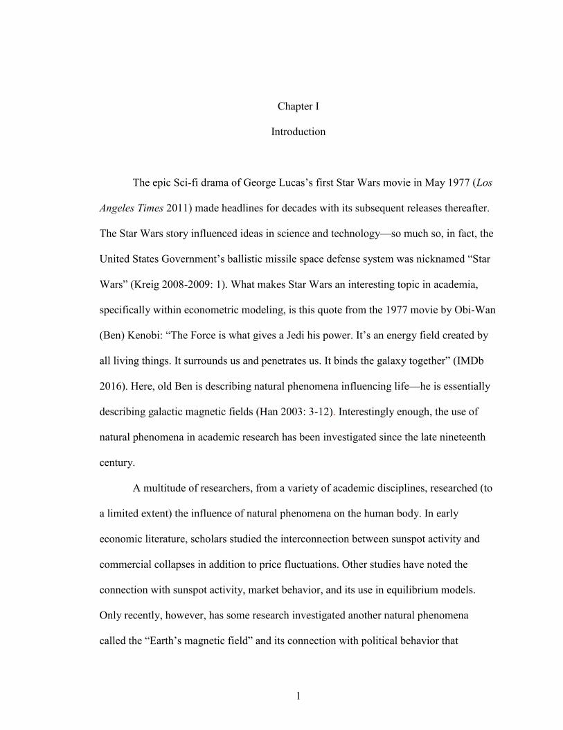
The epic Sci-fi drama of George Lucas’s first Star Wars movie in May 1977 (Los
Angeles Times 2011) made headlines for decades with its subsequent releases thereafter.
The Star Wars story influenced ideas in science and technology—so much so, in fact, the
United States Government’s ballistic missile space defense system was nicknamed “Star
Wars” (Kreig 2008-2009: 1). What makes Star Wars an interesting topic in academia,
specifically within econometric modeling, is this quote from the 1977 movie by Obi-Wan
(Ben) Kenobi: “The Force is what gives a Jedi his power. It’s an energy field created by
all living things. It surrounds us and penetrates us. It binds the galaxy together” (IMDb
2016). Here, old Ben is describing natural phenomena influencing life—he is essentially
describing galactic magnetic fields (Han 2003: 3-12). Interestingly enough, the use of
natural phenomena in academic research has been investigated since the late nineteenth
century.
A multitude of researchers, from a variety of academic disciplines, researched (to
a limited extent) the influence of natural phenomena on the human body. In early
economic literature, scholars studied the interconnection between sunspot activity and
commercial collapses in addition to price fluctuations. Other studies have noted the
connection with sunspot activity, market behavior, and its use in equilibrium models.
Only recently, however, has some research investigated another natural phenomena
called the “Earth’s magnetic field” and its connection with political behavior that

2
potentially influences the outcome of market behavior in quantitative modeling (East
2014: 193-195). With such a colorful array of literature spanning physics to psychology,
however, this thesis will not continue to investigate how sunspot activity impacts
quantifiable societal outcomes, but use the natural phenomena of Earth’s magnetic field
to understand its influence and predictive power.
Research Questions
Since there is a research gap associating the Earth’s magnetic field with market
activity, this research will attempt to answer the following questions:
1. Although research has revealed the potential interconnection of geomagnetic
activity with market behavior, could this natural phenomena actually increase the
prediction power of quantitative models?
2. What about the human behavioral element—does that play a role in econometric
modeling?
Research Hypotheses
This research hypothesizes that, based on existing literature, the Earth’s magnetic
field might have a minute influence on improving quantifiable estimated outputs.
Although it can be hypothesized that magnetic activity could influence human economic
behavior, the use of the human behavioral element in econometric modeling might also
reveal some changes in predicted outputs. Despite the possibility of these variables
having some influence in quantitative estimation, the purpose of the thesis is to provide
grounded analysis for a better understanding of this research area—and contribute

3
meaningful findings that could give rise to new research areas outside the scope of
financial economics.
The thesis uses quantitative techniques to determine the variables’ possible impact
in estimated outputs. Additionally, this analysis relies on historical time-series data used
by an array of academic disciplines and institutions: such as geophysics, the social
sciences, and governmental agencies.
Research Significance
The significance of the final outcome in this research should reveal (a) the
relationships between or among the variables used in this research; (b) the influence of
geomagnetic activity in econometric outputs; (c) lastly, the impact of human economic
behavior, with and without geomagnetic activity, in quantitative estimation.

4
Chapter II
Definition of Terms
Chapter II defines all data used in this research. Applications, such as RStudio
(including packages) and Microsoft Excel, was utilized for data transformations,
adjustments, analysis, and storage:
Kp Index (abbreviation:“SumKp”): an independent variable of the Earth’s Magnetic
Field activity derived from the K Planetary Index which is transformed from its 3-
hourly range to a monthly average (NOAA 2016). Due to the lack of data quality from
the United States National Oceanic and Atmospheric Administration (NOAA), this data
was retrieved from the British Geological Survey in the United Kingdom. Chapter V
discusses additional transformations for this variable.
Ap Index (abbreviation:“Ap”): an independent variable measuring geomagnetic storm
events in a 24-hour time period derived from the Kp Index which aligns, to some
degree, with sunspot activity (NOAA 2016). For this research, the Index was
transformed to a monthly average. Due to the lack of data quality from the United
States National Oceanic and Atmospheric Administration (NOAA), this data was
retrieved from the British Geological Survey in the United Kingdom. The data is also
transformed using a variety of mathematical techniques to test its impact on market
activity—this is discussed later in Chapter V.
Cp & C9 Index (abbreviation:“Cp” & “C9”): both Cp and C9 are independent variables
measuring overall magnetic activity. The C9 Index, however, converts the Cp Index to

5
a single digit from 0 to 9 (Ivory 2016: 1). These variables were converted to a monthly
average for this research. Since this data is not provided by the United States National
Oceanic and Atmospheric Administration (NOAA) at the time of retrieval, the British
Geological Survey in the United Kingdom served as an access-point for this
information. Chapter V discusses additional transformations for these variable.
Personal Consumption Expenditure (abbreviation:“PerConsumEx”): an independent
human economic behavior variable representing spending on goods and services within
the United States. This data frequency is monthly and seasonally adjusted with
additional data transformations discussed in Chapter V. The information was retrieved
from the Federal Reserve Bank of St. Louis.
Velocity of M2 Money Stock (abbreviation:“ M2Money”): an independent human
economic behavior variable representing all U.S. currency in circulation which includes
investment, savings, and deposit accounts. The data frequency is monthly in billions of
U.S. Dollars and seasonally adjusted. This information was retrieved from the Federal
Reserve Bank of St. Louis. Additional data transformations were conducted for this
research study (See Chapter V).
Personal Savings Rate (abbreviation:“PerSavRate”): an independent human economic
behavior variable describing the percentage rate at which U.S. citizens save their
money from disposable income. This data has a monthly frequency, is seasonally
adjusted, and in billions of U.S. Dollars. The data was provided by the Federal Reserve
Bank of St. Louis. Additional data transformations were conducted for this research
study (See Chapter V).

6
Unemployment (abbreviation:“U3Unemploy”): an independent human economic
behavior variable that represents seasonally adjusted U-3 unemployment rate in the
United States. The data frequency is monthly and retrieved from the United States
Bureau of Labor of Statistics. Additional data transformations were conducted for this
research study (See Chapter V).
MktRF, SMB, HML, RMW, and CMA: independent variables representing factors used
in Fama-French’s model: such as MktRF, also abbreviated as (Rmt – Rft), which
represents the return for the New York Stock Exchange (NYSE), NASDAQ, and the
American Stock Exchange (AMEX) minus the U.S. Treasury Bill rate (at one month);
SMB reflects the mean return from a small portfolio minus large portfolios; HML is
calculated by subtracting the high book-to-market to the Small B/M value on value
portfolios and growth portfolios; RMW is calculated by subtracting two robust
portfolios from two weak operating portfolios in term of their mean return; lastly,
CMA’s calculation is similar to RMW, but considers the level of risk tolerance by
subtracting high and low risk portfolios (French 2016: 1). These variables were
retrieved from Kenneth French’s website at the Tuck School of Business, Dartmouth
College.
STT: a dependent variable representing State Street Corporation’s monthly closed-
adjusted stock price to incorporate dividends and splits (NYSE: STT). The data was
retrieved from Yahoo Finance.
Van500: a dependent variable representing Vanguard’s S&P 500 Index fund
(NASDAQ: VFINX) that closely tracks the S&P 500 Index. The fund consists of the
largest American corporations which accounts for 75% of the U.S. stock market’s value

7
(Vanguard 2016). The data frequency is monthly and incorporates adjusted closed
domestic stock price to account for dividends and splits. This data was retrieved from
Yahoo Finance.

8
Chapter III
Literature Review − Background of the Problem
The first academic literature documenting the Earth’s Magnetic Field was
published by William Gilbert in De Magnete. Gilbert (1600/1958) discussed the Earth’s
magnetic field as a force controlling the North and South Pole. In addition, Gilbert
(1600/1958) also explained how the geomagnetic field dictates the behavior of a
compass’s needle in terms of the true North, South, East, and West that is dependent on
the geographical location of the measurement being observed or recorded.
Lanza & Meloni (2006) has noted that the Earth’s magnetic field is divided into
three parts: (1) the internal field, also known as the Main Field; (2) the magnetosphere,
which is the external field; and (3) the ionosphere, which is responsible for global
variation in magnetism on Earth. Although the origins of the geomagnetic field are still
being studied, the Main Field is produced by the Earth’s fluid core; in addition, the
external field (i.e., magnetosphere) is produced by electric currents protecting Earth from
solar wind dictated by the Sun’s behavior (Lanza & Meloni 2006: 1). According to the
National Oceanic and Atmospheric Administration (NOAA), the Earth’s magnetic field is
measured by the following:
declination (D), inclination (I), horizontal intensity (H), the north (X) and
east (Y) components of the horizontal intensity, vertical intensity (Z), and
total intensity (F). The parameters describing the direction of the magnetic
field are declination (D) and inclination (I). D and I are measured in units
of degrees, positive east for D and positive down for I. The intensity of the
total field (F) is described by the horizontal component (H), vertical
component (Z), and the north (X) and east (Y) components of the

9
horizontal intensity. These components may be measured in units of gauss
but are generally reported in nanoTesla (1nT * 100,000 = 1 gauss). The
Earth’s magnetic field intensity is roughly between 25,000 - 65,000 nT (.25
- .65 gauss). Magnetic declination is the angle between magnetic north and
true north. D is considered positive when the angle measured is east of true
north and negative when west. Magnetic inclination is the angle between
the horizontal plane and the total field vector, measured positive into Earth.
In older literature, the term “magnetic elements” often referred to D, I, and
H (NOAA 2016).
NOAA (2016) also measures the magnetic field with indices: such as [K], [KP], and
[AP]; the [K] Index represents a 3 hour range of magnetic activity; the [KP] Index is a
planetary mean measurement of the [K] Index; the [AP] Index is similar to the [KP]
Index in that it measures the earliest maximum value in a 24-hour time period. Lastly, the
[Cp] Index is a qualitative estimate of overall magnetic activity, which aggregates daily
[AP] measurements—this index also has a counterpart called the [C9] Index that converts
the [Cp] Index to one digit ranging from 0 to 9 (Ivory 2016: 1). With this knowledge, the
question is: how influential could magnetic activity be in quantitative modeling? Since
there is limited information on the subject, history has shown that researchers have used
natural phenomena in a variety of studies.
Hyde Clarke’s “A Preliminary Inquiry into the Physical Laws Governing the
Periods of Famines and Panics” was one of the first publications describing how a natural
phenomenon could be interconnected with economic activity. After Clarke (1847)
introduced the concept of “physical economy,” he compared cycles of crops including
price fluctuations, famine periods, the influence of solar and lunar winds on Earth’s
weather, and harvest periods. The result was that speculation, famine, and panic can
occur in roughly ten or eleven year intervals (Clarke 1847: 157). Outside factors, such as

10
solar and lunar winds influencing weather trends on Earth leading to economic
fluctuations, prompted an investigation into the physical laws of sunspot behavior.
In “Commercial Crisis and Sun-Spots,” Jevons referenced Hyde Clarke’s
exploration on how nature can influence economic outcomes. Jevons (1878) focused his
research on sunspot activity and commercial collapses; the end result from his study
revealed a 10.8 year interval in the commercial collapse timeline of 1825, 1836-9, 1847,
1857, and 1866; when comparing that interval with the duration of sunspot activity, the
results revealed a difference of 0.3.1 The discovery of business cycles linking with
sunspot activity led to a quantitative standard in the twentieth century.
“Do Sunspots Matter?” introduced the sunspot equilibrium formulated by Karl
Shell and David Cass in response to the 1878 study by Jevons. The purpose of this
equilibrium model was to deviate away from the traditional models that yielded certainty
equilibria to a broader and more non-traditional approach (Shell and Cass 1983: 195).
Shell and Cass’s final overall result was that sunspots are an extrinsic random variable
that do not influence general economic principles; the equilibrium, however, can offer an
explanation of excess volatility.
Bizer et al. (2014) produced one of the first and most recent experimental studies
which explored strategic coordination and sunspot activity in economic forecasting. The
final result was that accurate predictions were finite with low payoffs under this model.
1 The commercial collapse interval (10.8) was deducted by the sunspot interval
(10.5). This calculation was intended to show the difference between actual verses
predicted results.
11
Bizer et al. (2014) suggested that more research should be conducted to reduce herding
for forecasters to support anti-herding.
“Sunspots, GDP, and the Stock Market” used raw data from the National
Aeronautics and Space Administration (NASA) that recorded the number of sunspots
over time. They analyzed the moving average of sunspot behavior, the Dow Jones
Industrial Average (DJIA), and the U.S. gross domestic product. The concluding results
were that the correlation between these variables is insignificant. Modis (2007), however,
noted that sunspot activity and its unusual similarity with the DJIA and U.S. GDP
warrants further investigation by scholars.
Russian academics Belkin & Poluyakhtov investigated the relationship between
solar activity cycles (i.e., sunspots), real U.S. GDP, and interest rates in “Unconventional
Cyclical Theory: Cyclical Solar Activity and the Cyclical Development of the Economy.”
Data used in their research was the annual indexes of real U.S. GDP and the number of
Wolf W—an indicator of solar activity. Belkin & Poluyakhtov (2011) analyzed extreme
deviations from the mean solar cycle activity including maximums and minimums in
correlation with GDP and interest rate growth. Belkin & Poluyakhtov (2011) concluded
that solar activity and interest rates appear to be correlated with a coefficient of 79%. In
addition, the authors (2011) also noted a possible economic decline from 2013-2015.
“Unemployment, and Recessions, or Can the Solar Activity Cycle Shape the Business
Cycle?” revisited solar activity maximums and their correlation with U.S. recessions—
roughly seven solar maximums revealed eight out of thirteen recessions plus low U.S
unemployment being preceded by six solar maximums with a rapid increase of
unemployment following a two to three year lag. Gorbanev (2012) methodology used

12
monthly data of sunspot numbers from the National Aeronautics and Space
Administration (NASA) and the U.S. National Oceanic and Atmospheric Administration
(NOAA).
In 2014, Jakie R. East published the first political science dissertation on how
natural phenomena, such as the Sun and Earth, could not only have a connection with
economics, but human behavior entitled “Natural Phenomena as Potential Influence on
Social and Political Behavior: The Earth’s Magnetic Field.” East’s ( 2014) dissertation
analyzed the baseline relationship between geomagnetic frequencies and an array of
societal outcomes within several social science disciplines.
For Political Science and Criminology, East (2014) illustrated that one area of the
natural phenomena effect on human behavior was expressed by the “opportunity and
motivation theory” under SAD (Seasonal Affective Disorder), where higher temperatures
correlates with less crime and the lack of sunlight is associated with depression and
suicide that influences the melatonin and serotonin areas of the brain (East 2014: 14-15).
Sociology, Psychology, and Biology has predominantly used a number of natural
phenomena variables to explain human behavior derived from Charles Darwin’s idea of
natural selection (East 2014: 16-17). For example, East (2014) noted that the New
Ecological Paradigm (NEP) uses natural phenomena variables to explain how human
behavior might be influenced by this environment (East 2014: 17). In addition, subfields
of psychology, such as environmental and evolutionary, examines how human behavior
and the environment interact with each other (East 2014: 17-18).
Although Economics has not heavily researched how geophysical variables are
interconnected with human behavior, which in turn, to some degree, could influence

13
market fluctuations, East (2014) analyzed how the Earth’s magnetic field could explain
swings in market prices. More specifically, for daily low & high numbers in the stock
market, an escalation in the [y] and [h] component of the magnetic field tends to increase
the distance between high and low numbers (East 2014: 193). In addition, East (2014)
also used the AP Index of the magnetic field to refine a model that analyzes U.S.
Presidential messages and its influence on the Dow Jones Industrial Average (DJIA) and
the National Association of Securities Dealers Automated Quotations (NASDAQ) index;
in East’s (2014) analysis, the magnetic variable did, in fact, slightly refine Martin’s (2008)
model (East 2014: 197-200).
Other literature, authored by Babayev & Allahverdiyeva (2007), noted that severe
magnetic disturbances can cause negative human emotional responses. Palmer, Rycroft,
and Cermack (2006) revealed that extreme low or high geomagnetic activity could affect
melatonin levels and cardiovascular health. Karasek et al. (1998) also published a study
revealing the effect of magnetic fields on melatonin levels within the human brain. East
(2014) also cited the interconnection between magnetic activity and the human brain’s
melatonin and serotonin levels. To better understand how both natural phenomena (i.e.,
magnetic activity) and human behavior could potentially influence outputs in quantitative
modeling, the Fama-French model is reviewed.
William F. Sharpe introduced the theory of the Capital Pricing Asset Model
(CAPM) in 1964 entitled “Capital Asset Prices: A Theory of Market Equilibrium under
Conditions of Risk,” with later contributions by John Linter (1965a, b), Jack Treynor
(1962), and Jan Mossin (1966); the CAPM model is described as:
Er= rf + βi(Em – rf) (1)

14
where:
Es = Expected return,
Rf = Risk free rate,
βi = Sensitive of a security,
Em = Expected market return,
(Em – rf) = Risk premium.
This model calculates the expected (predicted) return of a security or portfolio. In
equilibrium, the total risk is not priced—instead, it is market risk (systematic); in addition
the model also takes on specific risk (i.e., β)—meaning risk of the asset being estimated.
CAPM eventually became a benchmark for later quantitative equations to estimate
(predict) possible returns.
Following the contribution from Sharpe (1964), Linter (1965a, b), Treynor
(1962), and Mossin (1966) was the introduction of the three-factor model by Eugene
Fama and Kenneth French (1992, 1993) extending the CAPM model; the Fama-French
(1992, 1993) regression model is represented by the following equation:
Rit – Rft = αi + βi(Rmt – Rft) + siSMB +hiHMLt +ϵit ;
t = 1, 2..T for each i = 1, 2…N (2)
where:
αi = Intercept of the regression line;
Rit = For period t, return on security or portfolio i;
Rft = Risk free return;
Rmt = Return on the value-weighted market portfolio;
βi = Sensitive of a security;
siSMB = Small minus big;
hiHMLt = High minus low B/M;
ϵit = Standard error of the estimate.
The extension of the CAPM model by Fama and French (1992, 1993) added two more
betas (β) to the equation: SMB and HML. HML (β2) is calculated by subtracting the high

15
book-to-market to the Small B/M value. The theory behind this Fama and French’s
(1992, 1993) beta allows the model to recognize additional risk exposure between growth
and valued stocks. For SMB (β3), this is calculated by the difference between small and
large stocks—Fama and French’s (1992, 1993) calculation is essentially trying to explain
excess returns on a portfolio by market capitalization making this beta a measure of size
risk—meaning that smaller firms are exposed to more risk due to their lack of
diversification.
Overall, these models are designed to predict an outcome based on market
behavior. Since there is literature suggesting the interconnection with geomagnetic
activity and its influence on human behavior, could this natural phenomena actually
increase the prediction power of this model? What about the human element—does that
play a role in econometric modeling? This research will attempt to answer these
questions and provide grounded analysis for real-world model owners.

16
Chapter IV
Research Methodology
The research design will use a scenario analysis with differing categories: such as
a direct, indirect, and alternative quantitative modeling approach for the Fama-French 3-
factor model—this analyzes any improvement of the original model’s prediction
capabilities—and investigates the possible impact of the added variables on expected
returns without the Fama-French’s 3-Factor Model. The output of expected (predicated)
returns also incorporates a two-fold comparative analysis for model performance—this
includes single stock returns (i.e., State Street Corporation) and fund returns representing
500 of America’s largest corporations closely tracking the S&P 500 Index (i.e., Vanguard
S&P 500 Index Fund). The reason for using the Vanguard S&P 500 Fund is because the
Fama-French model typically performs much stronger compared to the use of a single
stock due to most of the 3-factors being constructed on a microeconomic level—the Fund
is also used to better understand how added variables behave in a larger market
environment. These assets are analyzed to determine if the modeling approaches
mentioned below increase estimation performance of the original Fama-French output.
The following is the direct approach equation:
Rit = αi + βi(Rmt – Rft) + siSMB +hiHMLt + β4it + β5it + β6it + ϵit ;
t = 1, 2..T for each i = 1, 2…N (3)
where:
αi = Intercept of the regression line;
Rit = For period t, return on security or portfolio i;
Rft = Risk free return;

17
Rmt = Return on the value-weighted market portfolio;
βi = Sensitive of a security;
siSMB = Small minus big;
hiHMLt = High minus low B/M;
β4it = SumKp activity for period t;
β5it = AP activity for period t;
β6it = Cp activity for period t;
ϵit = Standard error of the estimate.
The direct approach equation with human economic behavior variables is as follows:
Rit = αi + βi(Rmt – Rft) + siSMB +hiHMLt + β4it + β5it + β6it + β7it + β8it + β9it +
β10it + ϵit ; t = 1, 2..T for each i = 1, 2…N (4)
where:
αi = Intercept of the regression line;
Rit = For period t, return on security or portfolio i;
Rft = Risk free return;
Rmt = Return on the value-weighted market portfolio;
βi = Sensitive of a security;
siSMB = Small minus big;
hiHMLt = High minus low B/M;
β4it = SumKp activity for period t;
β5it = AP activity for period t;
β6it = Cp activity for period t;
β7it = Personal Consumption Expenditure for period t;
β8it = Velocity of M2 Money Stock for period t;
β9it = Personal Savings Rate for period t;
β10it = U-3 Unemployment for period t;
ϵit = Standard error of the estimate.
Alternative Model 1 Equation:
Rit = αi + βi(Rmt – Rft) + siSMB +hiHMLt + ∆β4it + ∆β5it + ∆β6it + ϵit ;
t = 1, 2..T for each i = 1, 2…N (5)
where:
αi = Intercept of the regression line;
Rit = For period t, return on security or portfolio i;
Rft = Risk free return;

18
Rmt = Return on the value-weighted market portfolio;
βi = Sensitive of a security;
siSMB = Small minus big;
hiHMLt = High minus low B/M;
∆β4it = SumKp activity for period t;
∆β5it = AP activity for period t;
∆β6it = Cp activity for period t;
ϵit = Standard error of the estimate.
Alternative Model 2 Equation:
Rit = αi + βi(Rmt – Rft) + siSMB +hiHMLt + ∆β4it + ∆β5it + ∆β6it + ∆β7it + ∆β8it
+ ∆β9it + ∆β10it + ϵit ; t = 1, 2..T for each i = 1, 2…N (6)
where:
αi = Intercept of the regression line;
Rit = For period t, return on security or portfolio i;
Rft = Risk free return;
Rmt = Return on the value-weighted market portfolio;
βi = Sensitive of a security;
siSMB = Small minus big;
hiHMLt = High minus low B/M;
∆β4it = SumKp activity for period t;
∆β5it = AP activity for period t;
∆β6it = Cp activity for period t;
∆β7it = Personal Consumption Expenditure for period t;
∆β8it = Velocity of M2 Money Stock for period t;
∆β9it = Personal Savings Rate for period t;
∆β10it = U-3 Unemployment for period t;
ϵit = Standard error of the estimate.
Alternative Model 3 Equation:
Rit = αi + βi(Rmt – Rft) + siSMB +hiHMLt + ∆β4it + ∆β5it + ∆β6it + ∆β7it + ϵit ; t =
1, 2..T for each i = 1, 2…N (7)
where:
αi = Intercept of the regression line;
Rit = For period t, return on security or portfolio i;
19
Rft = Risk free return;
Rmt = Return on the value-weighted market portfolio;
βi = Sensitive of a security;
siSMB = Small minus big;
hiHMLt = High minus low B/M;
∆β4it = Personal Consumption Expenditure for period t;
∆β5it = Velocity of M2 Money Stock for period t;
∆β6it = Personal Savings Rate for period t;
∆β7it = U-3 Unemployment for period t;
ϵit = Standard error of the estimate.
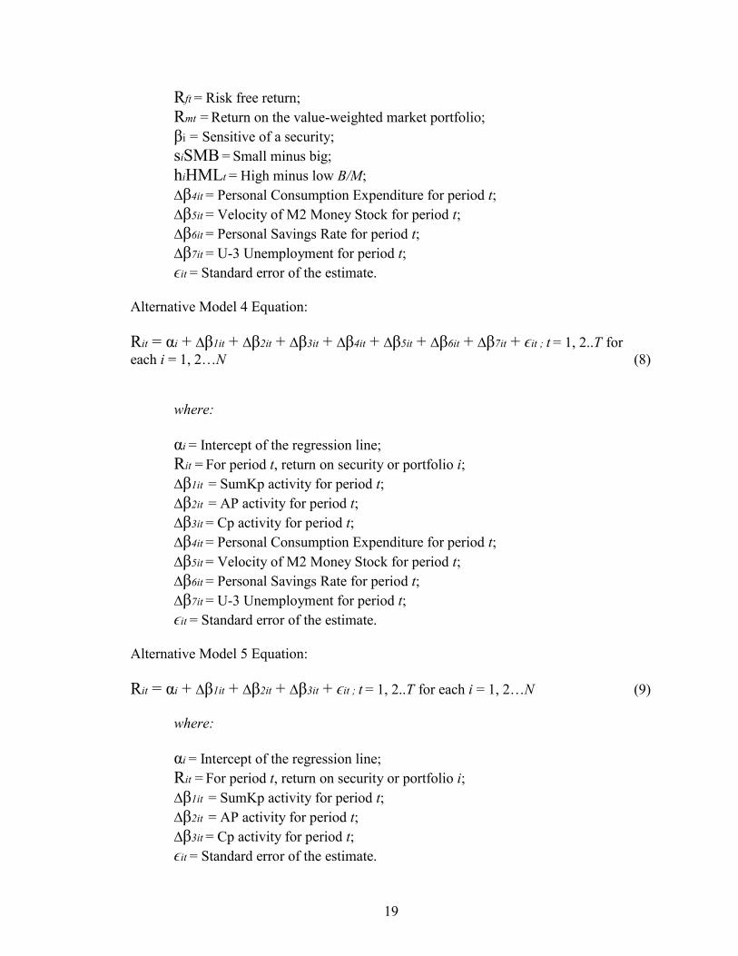
Alternative Model 4 Equation:
Rit = αi + ∆β1it + ∆β2it + ∆β3it + ∆β4it + ∆β5it + ∆β6it + ∆β7it + ϵit ; t = 1, 2..T for
each i = 1, 2…N (8)
where:
αi = Intercept of the regression line;
Rit = For period t, return on security or portfolio i;
∆β1it = SumKp activity for period t;
∆β2it = AP activity for period t;
∆β3it = Cp activity for period t;
∆β4it = Personal Consumption Expenditure for period t;
∆β5it = Velocity of M2 Money Stock for period t;
∆β6it = Personal Savings Rate for period t;
∆β7it = U-3 Unemployment for period t;
ϵit = Standard error of the estimate.
Alternative Model 5 Equation:
Rit = αi + ∆β1it + ∆β2it + ∆β3it + ϵit ; t = 1, 2..T for each i = 1, 2…N (9)
where:
αi = Intercept of the regression line;
Rit = For period t, return on security or portfolio i;
∆β1it = SumKp activity for period t;
∆β2it = AP activity for period t;
∆β3it = Cp activity for period t;
ϵit = Standard error of the estimate.
20
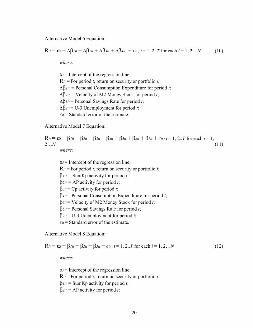
Alternative Model 6 Equation:
Rit = αi + ∆β1it + ∆β2it + ∆β3it + ∆β4it + ϵit ; t = 1, 2..T for each i = 1, 2…N (10)
where:
αi = Intercept of the regression line;
Rit = For period t, return on security or portfolio i;
∆β1it = Personal Consumption Expenditure for period t;
∆β2it = Velocity of M2 Money Stock for period t;
∆β3it = Personal Savings Rate for period t;
∆β4it = U-3 Unemployment for period t;
ϵit = Standard error of the estimate.
Alternative Model 7 Equation:
Rit = αi + β1it + β2it + β3it + β4it + β5it + β6it + β7it + ϵit ; t = 1, 2..T for each i = 1,
2…N (11) where:
αi = Intercept of the regression line;
Rit = For period t, return on security or portfolio i;
β1it = SumKp activity for period t;
β2it = AP activity for period t;
β3it = Cp activity for period t;
β4it = Personal Consumption Expenditure for period t;
β5it = Velocity of M2 Money Stock for period t;
β6it = Personal Savings Rate for period t;
β7it = U-3 Unemployment for period t;
ϵit = Standard error of the estimate.
Alternative Model 8 Equation:
Rit = αi + β1it + β2it + β3it + ϵit ; t = 1, 2..T for each i = 1, 2…N (12)
where:
αi = Intercept of the regression line;
Rit = For period t, return on security or portfolio i;
β1it = SumKp activity for period t;
β2it = AP activity for period t;

21
β3it = Cp activity for period t;
ϵit = Standard error of the estimate.
Alternative Model 9 Equation:
Rit = αi + β1it + β2it + β3it + β4it + ϵit ; t = 1, 2..T for each i = 1, 2…N (13)
where:
αi = Intercept of the regression line;
Rit = For period t, return on security or portfolio i;
β1it = Personal Consumption Expenditure for period t;
β2it = Velocity of M2 Money Stock for period t;
β3it = Personal Savings Rate for period t;
β4it = U-3 Unemployment for period t;
ϵit = Standard error of the estimate.
In addition to the original modeling approach noted above, the research also utilizes two
other frameworks: such as the data transformation and exponential moving average
(EMA) approach. The transformation approach (see Appendix B) uses existing data to
better understand if any real impact may be viable for quantitative estimation; the data
transformation approach, however, will not use models located in the original approach.
Moreover, since geomagnetic data tends to be noisy, added betas are re-calculated to their
EMA form—human economic behavioral data is also transformed to understand their
impact in quantitative estimation. In addition, since both Cp and C9 are measurements of
the same geomagnetic frequency (with differing approaches), only Cp is utilized due to a
slight positive correlation increase with State Street stock returns—the same approach is
also applied to the Vanguard S&P 500 Fund. Lastly, data is correlated, using Pearson’s
correlation, to determine if any relationships exists between or among independent and
dependent variables (see Appendix D & E).

22
The variable selection process will have a p-value cap of 5%; a variance inflation
factor (VIF) analysis is also conducted to ensure that the selected variables are not
inflating model fitness metrics and to reduce multicollinearity; if a VIF analysis reveals
severe inflation, the removal of the variable will likely occur. Autocorrelation will be
addressed on a case-by-case basis—if severity is detected, generalized least square
regression or dependent variable differencing might occur. Data with the strongest
dependent variable relationship and model fit is tested against the Fama-French’s original
model (see Chapter VIII) to determine if there is any quantitative estimation
improvement—this includes conducting an analysis comparing actual verses estimated
outcomes to determine the model’s true reliability of predicted returns. Additionally, a
robustness analysis, during the 2008-2009 Financial Crisis, is used to test whether the
selected models can predict swings in the market. Lastly, human economic behavioral
and geomagnetic variables are tested for causality using the Granger test (see Appendix
C)—this is to determine if there are any underlying relationships among human
behavioral economic and geomagnetic variables (Granger 1988: 199-211). Although it is
not known if these variables reveal a relationship with each other for a predicted
outcome, it could be hypothesized that the unknown and known measurement error for
the time-series regression models should not reveal a significance of - 0 -.

23
Chapter V
Data Transformations
All variables used in Chapter II have undergone data transformations outside the
scope of absolute delta to better understand their impact in predicting returns; although a
select number of variables have already undergone a seasonality transformation from
their original source, this research did not adjust for seasonality. Table 5-1 below
illustrates the equation used to transform each independent variable including its name
and variable description ranging from September 1986 to November 2014.
Table 5-1: Data Transformations
Variable Name Variable
Equation Variable Description
PerConsumExDelta X2t - X1t
Personal Consumptions Expenditure transformed to express
the change (∆) from the current rate in time X2t minus the
previous rate X1t.
M2MoneyDelta X2t - X1t Velocity of Money transformed to express the change (∆)
from the current rate in time X2t minus the previous rate X1t.
PerSavDelta X2t - X1t Personal Savings Rate transformed to express the change (∆)
from the current rate in time X2t minus the previous rate X1t.
U3UnemployDelta X2t - X1t
U-3 unemployment rate transformed to express the change
(∆) from the current rate in time X2t minus the previous rate
X1t.
Kppwhalf √Xt The KP Index datum is square-rooted .
KPLN Ln(Xt) The KP Index datum transformed to its natural-logarithm.
SumKPDelta X2t - X1t The KP Index transformed to express the change (∆) from the
current rate in time X2t minus the previous rate X1t.
SumKPInv 1 ÷ Xt 1 divides the KP Index datum.
SumKPInvDelta X2t - X1t The derivative of SumKPInv transformed to express the
change (∆) from the current rate in time X2t minus the

24
previous rate X1t.
Appw8 Xt(1/0.8) The AP Index datum is squared by 1/0.8.
ApLn Ln(Xt) The AP Index datum transformed to its natural-logarithm.
APSqrt √ Xt The AP Index datum square-rooted for the data series.
APDelta X2t - X1t
The AP Index data series transformed to express the change
(∆) from the current rate in time X2t minus the previous rate
X1t.
APInv 1 ÷ Xt 1 divides the AP Index datum.
APInvDelta X2t - X1t
The derivative of APInv transformed to express the change
(∆) from the current rate in time X2t minus the previous rate
X1t.
Cppwnine Xt(1/9) The CP Index datum is squared by 1/9.
CpLn Ln(Xt) The CP Index datum transformed to its natural-logarithm.
CpSqrt √ Xt The CP Index datum square-rooted for the data series.
CPDelta X2t - X1t
The CP Index data series transformed to express the change
(∆) from the current rate in time X2t minus the previous rate
X1t.
CpInv 1 ÷ Xt 1 divides the CP index datum.
CpInvDelta X2t - X1t
The derivative of CpInv transformed to express the change
(∆) from the current rate in time X2t minus the previous rate
X1t.
C9pwsqurt Xt(2) The C9 Index datum is squared.
C9Ln Ln(Xt) The C9 Index datum transformed to its natural-logarithm.
C9Squrt √ Xt The C9 Index datum square-rooted for the data series.
C9Delta X2t - X1t
The C9 Index data series transformed to express the change
(∆) from the current rate in time X2t minus the previous rate
X1t.
C9Inv 1 ÷ Xt 1 divides the C9 Index datum.
C9InvDelta X2t - X1t
The derivative of C9Inv transformed to express the change
(∆) from the current rate in time X2t minus the previous rate
X1t.
25
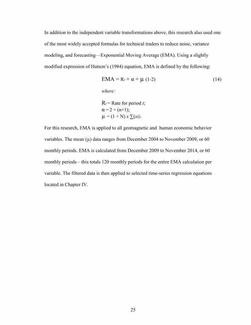
In addition to the independent variable transformations above, this research also used one
of the most widely accepted formulas for technical traders to reduce noise, variance
modeling, and forecasting—Exponential Moving Average (EMA). Using a slightly
modified expression of Hutson’s (1984) equation, EMA is defined by the following:
EMA = Rt + α + µ (1-2) (14)
where:
Rt = Rate for period t;
α = 2 ÷ (n+1);
µ = (1 ÷ N) x ∑(xi).
For this research, EMA is applied to all geomagnetic and human economic behavior
variables. The mean (µ) data ranges from December 2004 to November 2009, or 60
monthly periods. EMA is calculated from December 2009 to November 2014, or 60
monthly periods—this totals 120 monthly periods for the entire EMA calculation per
variable. The filtered data is then applied to selected time-series regression equations
located in Chapter IV.

26
Chapter VI
Limitations
This research design is limited by advanced knowledge of geophysics. Since there
are multiple variables involved outside the scope of this design, it would be improbable
to identity every aspect and element influencing the research outcome. Moreover, the use
of more advanced quantitative techniques, such as vector autoregression (VAR)
modeling, is limited. Research limitations may also extends to medical and psychology
research used to evaluate and explain human behavior. In addition, this research is
limited to the 13 observatories measuring magnetic activity worldwide. Human economic
behavior data is limited to the United States. Data quality is limited to selected sources
mentioned in this research and cannot guarantee 100% accuracy of the raw data used.
The processing component is limited to least squares regression due to Fama and
French’s methodology choice; moreover, time-series data is not adjusted for lag. Models
that use Fama-French factors may only be applied to the equities market, or funds
constructed with stocks due to the research approach used. If the model(s) does not
include Fama-French factors, this research may only be applied to asset classes being
bought or sold in economies comparable with the United States—this is due to the nature
of the data being used in the analysis.
27
Chapter VII
Quantitative Modeling with Returns
Chapter VII is comprised of all time-series regression model approaches using
data in the original approach illustrated on Chapter IV and EMA filtered data for both
State Street Corporation’s stock and the Vanguard S&P 500 Index Fund percent-returns;
correlation matrices are located in Appendix D to E.
Original Approach: State Street Corporation Stock Returns
This section uses all equations (3 – 13) located in Chapter IV. After all regression
outputs have been calculated with the selected data, the model’s parameters maybe
modified (if applicable) to meet the cut-off p-value of any measurement over 5%. The
monthly time-series range is from October 1986 to November 2014. The first table
reveals regression results for the Direct Model Equation 3 (“DirectModel”) and the
direct model with human economic behavior variables, Equation 4 (“DirectModelEcon”)
compared with the Fama-French model (“FFModel”) using State Street Corporation
adjusted stock returns. For variable elimination, the focus of the regression output
includes the following: (i) Adj. R2, (ii) RMSE (root-mean-squared-error), and (iii) p-
values (0.1%, 1%, or 5%). A variance inflation factor (VIF) analysis will typically occur
after the model’s parameters have been adjusted.

28
Table 7-1: STT Original Model Regression Results, Part 1
In both the DirectModel and DirectModelEcon, added variables have reduced the
models’ goodness-of-fit compared the FFModel by the decrease in Adj. R2. In addition,
RMSE has increased compared to the FFModel which suggests that these models have
less predictability. All added variables compared to the original FFModel have a p-value
above 5% regardless if they were tested separately or together—this suggests a weak
relationship with State Street Corporation’s stock return. In the DirectModel equation,
aggregating all geomagnetic indices creates multicollinearity with variance inflation
factors (VIF) ranging from 14 (min) to 502 (max). DirectModelEcon, which includes
both geomagnetic and human economic variables, revealed that the economic parameters
DirectModel DirectModelEcon FFModel
===============================================
(Intercept) 0.23272 0.97533 -0.06705
(0.86118) (1.29853) (0.13014)
MktRF 0.36905 *** 0.37291 *** 0.36832 ***
(0.02981) (0.02994) (0.02967)
SMB -0.09371 * -0.09492 * -0.09350 *
(0.04258) (0.04299) (0.04236)
HML 0.21288 *** 0.21666 *** 0.21147 ***
(0.04670) (0.04671) (0.04613)
SumKp -0.01097 -0.00385
(0.01889) (0.01983)
Ap 0.00214 -0.00456
(0.06268) (0.06380)
Cp 2.75657 1.81069
(4.86835) (5.10027)
PerConsumEx -0.00029
(0.00031)
M2Money 0.0004
(0.00031)
PerSavRate -0.11966
(0.14328)
U3Unemploy -0.13806
(0.12954)
-------------------------------------------------------------------------------
R^2 0.32797 0.33967 0.32647
Adj. R^2 0.31579 0.31948 0.32042
Num. obs. 338 338 338
RMSE 2.3617 2.35532 2.3537
===============================================
*** p < 0.001, ** p < 0.01, * p < 0.05

29
have inflation factors at 49 and 40 for personal consumption expeditors (PerConsumEx)
including money velocity (M2Money)—the results suggest that severe multicollinearity
exists when these parameters are used. The Fama-French model is the best model for
predicting State Street stock returns under this scenario based on Adj. R2, RMSE, and
probability values. Table 7-2 displays results for models 1 to 3 which includes the
absolute change (delta) in both geomagnetic and human economic behavior.
Table 7-2: STT Original Model Regression Results, Part 2
Model 1 Model 2 Model 3 FFModel
==========================================================
(Intercept) -0.06662 -0.05318 0.15167 -0.06705
(0.13064) (0.21847) (0.59268) (0.13014)
MktRF 0.36615 *** 0.36058 *** 0.36019 *** 0.36832 ***
(0.02995) (0.03035) (0.08190) (0.02967)
SMB -0.09061 * -0.10563 * 0.04623 -0.09350 *
(0.04272) (0.04336) (0.11671) (0.04236)
HML 0.21403 *** 0.20961 *** 0.31496 * 0.21147 ***
(0.04669) (0.04716) (0.12686) (0.04613)
SumKPDelta -0.00727 -0.00953
(0.02919) (0.02930)
APDelta -0.01159 -0.00677
(0.05243) (0.05248)
CPDelta 1.38283 1.73015
(6.10560) (6.12231)
PerConsumExDelta 0.00619 -0.01094
(0.00446) (0.01206)
M2MoneyDelta -0.00652 0.01342
(0.00471) (0.01270)
PerSavDelta 0.00559 -0.17342
(0.16921) (0.45808)
U3UnemployDelta 0.68023 -2.66238
(0.84619) (2.28092)
--------------------------------------------------------------------------------------------------
R^2 0.32746 0.33676 0.07174 0.32647
Adj. R^2 0.31527 0.31648 0.05211 0.32042
Num. obs. 338 338 339 338
RMSE 2.3626 2.36052 6.40795 2.3537
==========================================================
*** p < 0.001, **p < 0.01, * p < 0.05
Both models 1 and 2 has decreased performance compared to the Fama-French
model. Multicollinearity exists when geomagnetic indices are used in Model 1: such as
30
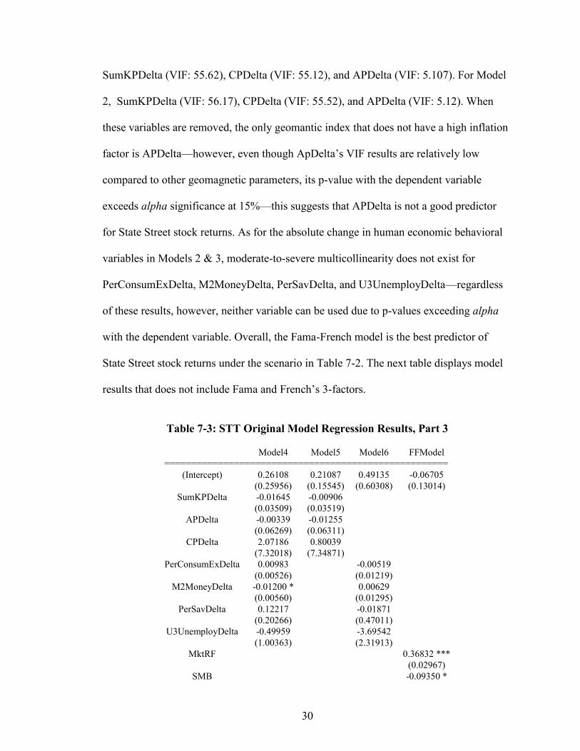
SumKPDelta (VIF: 55.62), CPDelta (VIF: 55.12), and APDelta (VIF: 5.107). For Model
2, SumKPDelta (VIF: 56.17), CPDelta (VIF: 55.52), and APDelta (VIF: 5.12). When
these variables are removed, the only geomantic index that does not have a high inflation
factor is APDelta—however, even though ApDelta’s VIF results are relatively low
compared to other geomagnetic parameters, its p-value with the dependent variable
exceeds alpha significance at 15%—this suggests that APDelta is not a good predictor
for State Street stock returns. As for the absolute change in human economic behavioral
variables in Models 2 & 3, moderate-to-severe multicollinearity does not exist for
PerConsumExDelta, M2MoneyDelta, PerSavDelta, and U3UnemployDelta—regardless
of these results, however, neither variable can be used due to p-values exceeding alpha
with the dependent variable. Overall, the Fama-French model is the best predictor of
State Street stock returns under the scenario in Table 7-2. The next table displays model
results that does not include Fama and French’s 3-factors.
Table 7-3: STT Original Model Regression Results, Part 3
Model4 Model5 Model6 FFModel
=====================================================
(Intercept) 0.26108 0.21087 0.49135 -0.06705
(0.25956) (0.15545) (0.60308) (0.13014)
SumKPDelta -0.01645 -0.00906
(0.03509) (0.03519)
APDelta -0.00339 -0.01255
(0.06269) (0.06311)
CPDelta 2.07186 0.80039
(7.32018) (7.34871)
PerConsumExDelta 0.00983 -0.00519
(0.00526) (0.01219)
M2MoneyDelta -0.01200 * 0.00629
(0.00560) (0.01295)
PerSavDelta 0.12217 -0.01871
(0.20266) (0.47011)
U3UnemployDelta -0.49959 -3.69542
(1.00363) (2.31913)
MktRF 0.36832 ***
(0.02967)
SMB -0.09350 *
31
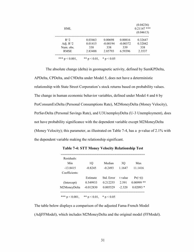
The absolute change (delta) in geomagnetic activity, defined by SumKPDelta,
APDelta, CPDelta, and C9Delta under Model 5, does not have a deterministic
relationship with State Street Corporation’s stock returns based on probability values.
The change in human economic behavior variables, defined under Model 4 and 6 by
PerConsumExDelta (Personal Consumptions Rate), M2MoneyDelta (Money Velocity),
PerSavDelta (Personal Savings Rate), and U3UnemployDelta (U-3 Unemployment), does
not have probability significance with the dependent variable except M2MoneyDelta
(Money Velocity); this parameter, as illustrated on Table 7-4, has a p-value of 2.1% with
the dependent variable making the relationship significant.
Table 7-4: STT Money Velocity Relationship Test
The table below displays a comparison of the adjusted Fama-French Model
(AdjFFModel), which includes M2MoneyDelta and the original model (FFModel).
(0.04236)
HML 0.21147 ***
(0.04613)
-----------------------------------------------------------------------------------------
R^2 0.03463 0.00698 0.00816 0.32647
Adj. R^2 0.01415 -0.00194 -0.00372 0.32042
Num. obs. 338 338 339 338
RMSE 2.83488 2.85793 6.59396 2.3537
=====================================================
*** p < 0.001, ** p < 0.01, * p < 0.05
===============================================
Residuals:
Min 1Q Median 3Q Max
-13.8415 -0.8245 -0.2493 1.1647 11.1416
Coefficients:
Estimate Std. Error t value Pr(>|t|)
(Intercept) 0.549933 0.212255 2.591 0.00999 **
M2MoneyDelta -0.012830 0.005529 -2.320 0.02093 *
===============================================
*** p < 0.001, ** p < 0.01, * p < 0.05

32
Table 7-5: STT Adjusted FFModel v. Original
AdjFFModel FFModel
=================================
(Intercept) 0.11346 -0.06705
(0.18044) (0.13014)
MktRF 0.36421 *** 0.36832 ***
(0.02975) (0.02967)
SMB -0.09746 * -0.09350 *
(0.04238) (0.04236)
HML 0.20425 *** 0.21147 ***
(0.04633) (0.04613)
M2MoneyDelta -0.00667
(0.00463)
--------------------------------------------------------
R^2 0.33065 0.32647
Adj. R^2 0.32261 0.32042
Num. obs. 338 338
RMSE 2.34991 2.3537
=================================
*** p < 0.001, ** p < 0.01, * p < 0.05
Although the p-value for M2MoneyDelta is no longer significant due to inflation
from other parameters, the Adj. R2 and RMSE appears to have slightly improved model
performance at 32.26% (AdjFFModel) verses 32.04% (FFModel)—RMSE at 2.35
(AdjFFModel) verses 2.353 (FFModel). For all variables in the alternative model,
variance inflation factors are within reasonability at 1.09 (MktRF), 1.13 (SMB), 1.14
(HML), and 1.03 (M2MoneyDelta). The intercept of AdjFFModel suggests that the
expected State Street single stock return rate is 11% per month; the slope can be viewed
as the expected one-unit per share stock increase results in an escalation of MktRF’s
coefficient by 0.36, SMB by -0.097, and HML by 0.20 with the change in money velocity
by -0.006, respectively. The Fama-French model reveals that the expected State Street
single stock return rate decreases 7% per month; the slope can be viewed as the expected
one-unit per share stock return decrease results in an increase of MktRF’s coefficient by
33
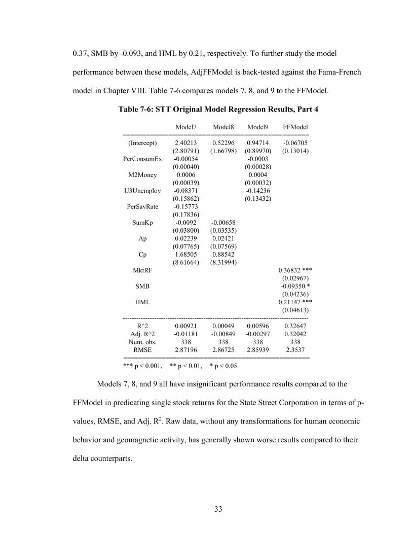
0.37, SMB by -0.093, and HML by 0.21, respectively. To further study the model
performance between these models, AdjFFModel is back-tested against the Fama-French
model in Chapter VIII. Table 7-6 compares models 7, 8, and 9 to the FFModel.
Table 7-6: STT Original Model Regression Results, Part 4
Model7 Model8 Model9 FFModel
=================================================
(Intercept) 2.40213 0.52296 0.94714 -0.06705
(2.80791) (1.66798) (0.89970) (0.13014)
PerConsumEx -0.00054 -0.0003
(0.00040) (0.00028)
M2Money 0.0006 0.0004
(0.00039) (0.00032)
U3Unemploy -0.08371 -0.14236
(0.15862) (0.13432)
PerSavRate -0.15773
(0.17836)
SumKp -0.0092 -0.00658
(0.03800) (0.03535)
Ap 0.02239 0.02421
(0.07765) (0.07569)
Cp 1.68505 0.88542
(8.61664) (8.31994)
MktRF 0.36832 ***
(0.02967)
SMB -0.09350 *
(0.04236)
HML 0.21147 ***
(0.04613)
-----------------------------------------------------------------------------------
R^2 0.00921 0.00049 0.00596 0.32647
Adj. R^2 -0.01181 -0.00849 -0.00297 0.32042
Num. obs. 338 338 338 338
RMSE 2.87196 2.86725 2.85939 2.3537
=================================================
*** p < 0.001, ** p < 0.01, * p < 0.05
Models 7, 8, and 9 all have insignificant performance results compared to the
FFModel in predicating single stock returns for the State Street Corporation in terms of p-
values, RMSE, and Adj. R2. Raw data, without any transformations for human economic
behavior and geomagnetic activity, has generally shown worse results compared to their
delta counterparts.
34
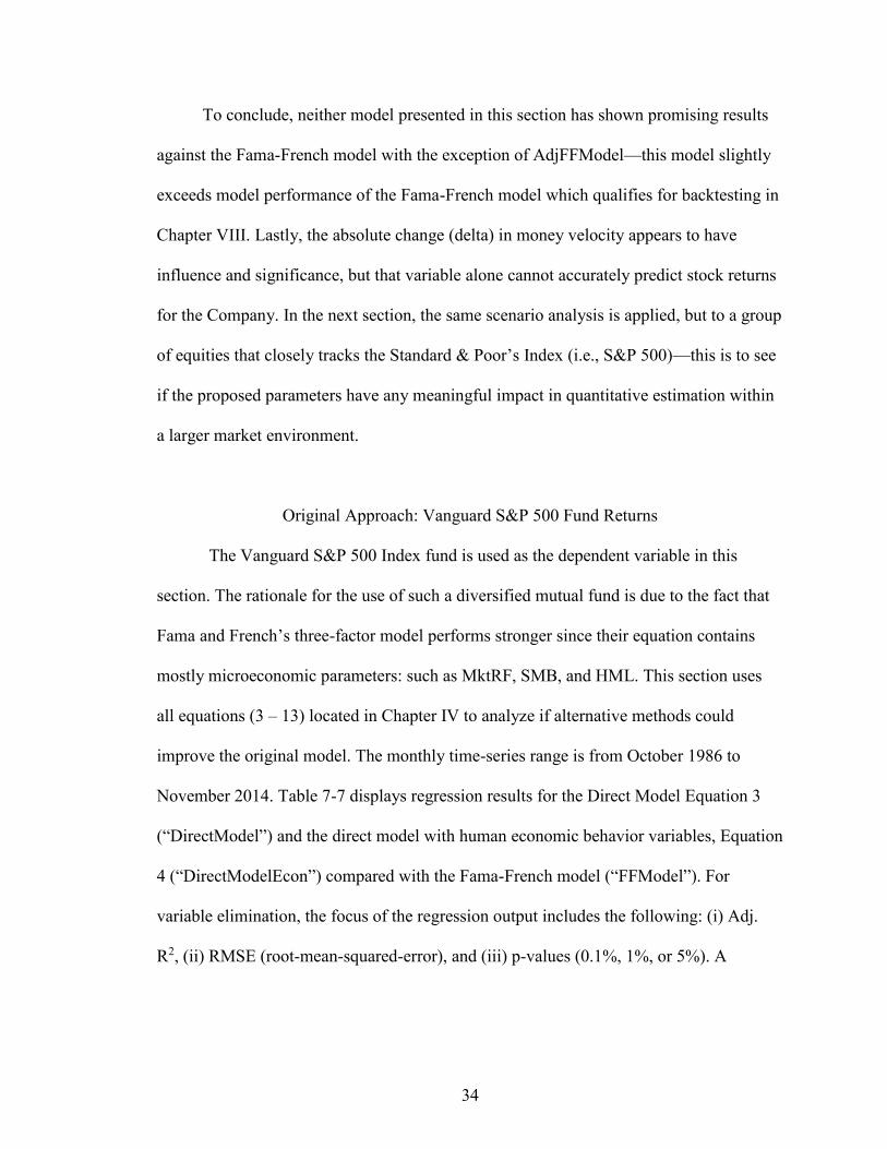
To conclude, neither model presented in this section has shown promising results
against the Fama-French model with the exception of AdjFFModel—this model slightly
exceeds model performance of the Fama-French model which qualifies for backtesting in
Chapter VIII. Lastly, the absolute change (delta) in money velocity appears to have
influence and significance, but that variable alone cannot accurately predict stock returns
for the Company. In the next section, the same scenario analysis is applied, but to a group
of equities that closely tracks the Standard & Poor’s Index (i.e., S&P 500)—this is to see
if the proposed parameters have any meaningful impact in quantitative estimation within
a larger market environment.
Original Approach: Vanguard S&P 500 Fund Returns
The Vanguard S&P 500 Index fund is used as the dependent variable in this
section. The rationale for the use of such a diversified mutual fund is due to the fact that
Fama and French’s three-factor model performs stronger since their equation contains
mostly microeconomic parameters: such as MktRF, SMB, and HML. This section uses
all equations (3 – 13) located in Chapter IV to analyze if alternative methods could
improve the original model. The monthly time-series range is from October 1986 to
November 2014. Table 7-7 displays regression results for the Direct Model Equation 3
(“DirectModel”) and the direct model with human economic behavior variables, Equation
4 (“DirectModelEcon”) compared with the Fama-French model (“FFModel”). For
variable elimination, the focus of the regression output includes the following: (i) Adj.
R2, (ii) RMSE (root-mean-squared-error), and (iii) p-values (0.1%, 1%, or 5%). A

35
variance inflation factor (VIF) analysis will typically occur after the model’s parameters
have been adjusted.
Table 7-7: Van500 Original Model Regression Results, Part 1
The DirectModel produces model performance results that is similar to the
FFModel by Adj. R2 and RMSE; however, after testing for significance at 5% or below
(Tables 7-8 to 7-10) with geomagnetic variables located below, these variables produce
inflated model performance metrics.
DirectModel DirectModelEcon FFModel
===============================================
(Intercept) -0.00290 0.00718 0.00257 ***
(0.00330) (0.00538) (0.00032)
MktRF 0.01005 *** 0.01006 *** 0.01004 ***
(0.00007) (0.00007) (0.00007)
SMB -0.00196 *** -0.00192 *** -0.00195 ***
(0.00010) (0.00010) (0.00010)
HML 0.00026 * 0.00024 * 0.00027 *
(0.00011) (0.00011) (0.00011)
SumKp 0.00008 -0.00002
(0.00007) (0.00007)
Ap -0.00001 0.00014
(0.00015) (0.00015)
Cp -0.01374 0.00075
(0.01649) (0.01650)
PerConsumEx 0.00000
0.00000
M2Money 0.00000
0.00000
PerSavRate 0.00052
(0.00034)
U3Unemploy -0.00087 **
(0.00030)
-------------------------------------------------------------------------------
R^2 0.98399 0.98521 0.98361
Adj. R^2 0.9837 0.98476 0.98347
Num. obs. 338 338 338
RMSE 0.00566 0.00547 0.0057
===============================================
*** p < 0.001, ** p < 0.01, * p < 0.05
36
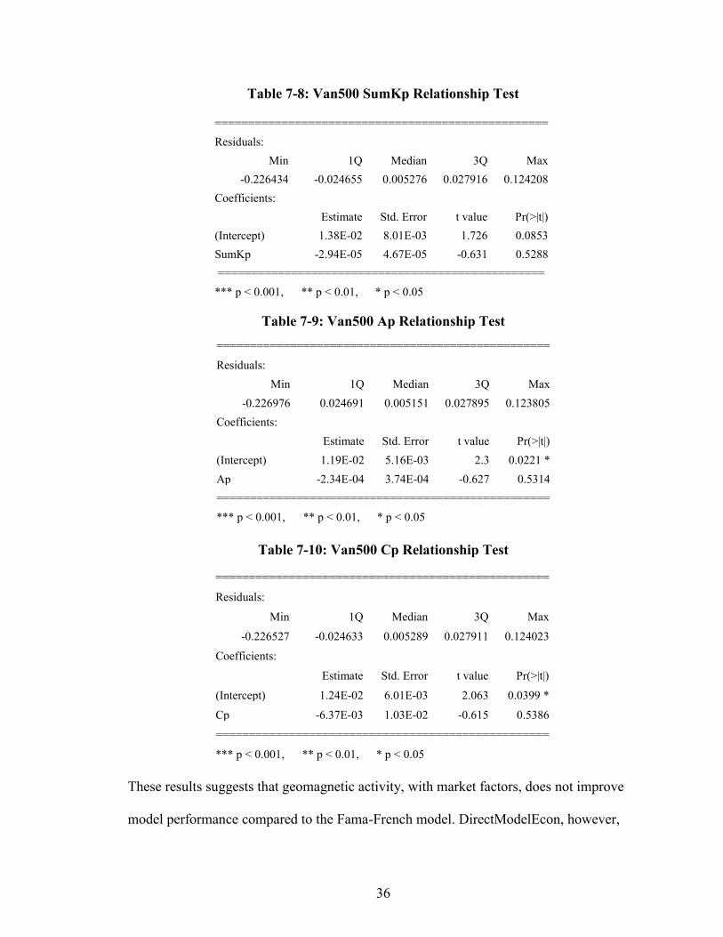
Table 7-8: Van500 SumKp Relationship Test
==================================================
Residuals:
Min 1Q Median 3Q Max
-0.226434 -0.024655 0.005276 0.027916 0.124208
Coefficients:
Estimate Std. Error t value Pr(>|t|)
(Intercept) 1.38E-02 8.01E-03 1.726 0.0853
SumKp -2.94E-05 4.67E-05 -0.631 0.5288
=================================================
*** p < 0.001, ** p < 0.01, * p < 0.05
Table 7-9: Van500 Ap Relationship Test
Table 7-10: Van500 Cp Relationship Test ==================================================
Residuals:
Min 1Q Median 3Q Max
-0.226527 -0.024633 0.005289 0.027911 0.124023
Coefficients:
Estimate Std. Error t value Pr(>|t|)
(Intercept) 1.24E-02 6.01E-03 2.063 0.0399 *
Cp -6.37E-03 1.03E-02 -0.615 0.5386
==================================================
*** p < 0.001, ** p < 0.01, * p < 0.05
These results suggests that geomagnetic activity, with market factors, does not improve
model performance compared to the Fama-French model. DirectModelEcon, however,
==================================================
Residuals:
Min 1Q Median 3Q Max
-0.226976 0.024691 0.005151 0.027895 0.123805
Coefficients:
Estimate Std. Error t value Pr(>|t|)
(Intercept) 1.19E-02 5.16E-03 2.3 0.0221 *
Ap -2.34E-04 3.74E-04 -0.627 0.5314
==================================================
*** p < 0.001, ** p < 0.01, * p < 0.05
37
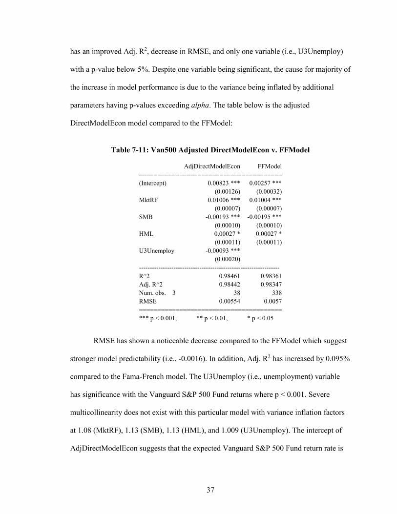
has an improved Adj. R2, decrease in RMSE, and only one variable (i.e., U3Unemploy)
with a p-value below 5%. Despite one variable being significant, the cause for majority of
the increase in model performance is due to the variance being inflated by additional
parameters having p-values exceeding alpha. The table below is the adjusted
DirectModelEcon model compared to the FFModel:
Table 7-11: Van500 Adjusted DirectModelEcon v. FFModel
RMSE has shown a noticeable decrease compared to the FFModel which suggest
stronger model predictability (i.e., -0.0016). In addition, Adj. R2 has increased by 0.095%
compared to the Fama-French model. The U3Unemploy (i.e., unemployment) variable
has significance with the Vanguard S&P 500 Fund returns where p < 0.001. Severe
multicollinearity does not exist with this particular model with variance inflation factors
at 1.08 (MktRF), 1.13 (SMB), 1.13 (HML), and 1.009 (U3Unemploy). The intercept of
AdjDirectModelEcon suggests that the expected Vanguard S&P 500 Fund return rate is
AdjDirectModelEcon FFModel
=======================================
(Intercept) 0.00823 *** 0.00257 ***
(0.00126) (0.00032)
MktRF 0.01006 *** 0.01004 ***
(0.00007) (0.00007)
SMB -0.00193 *** -0.00195 ***
(0.00010) (0.00010)
HML 0.00027 * 0.00027 *
(0.00011) (0.00011)
U3Unemploy -0.00093 ***
(0.00020)
-----------------------------------------------------------------
R^2 0.98461 0.98361
Adj. R^2 0.98442 0.98347
Num. obs. 3 38 338
RMSE 0.00554 0.0057
=======================================
*** p < 0.001, ** p < 0.01, * p < 0.05
38
0.82% (USD) per month; the slope can be viewed as the expected one-unit fund return
increase, per month, results in an escalation of MktRF’s coefficient by 0.01, SMB by -
0.001, and HML by 0.0002 with U-3 unemployment by -0.006, respectively. The Fama-
French model reveals that the expected Vanguard fund return rate is an increase of 0.26%
(USD) per month; the slope can be viewed as the expected one-unit Fund return increase,
per month, results in an escalation of MktRF’s coefficient by 0.01, SMB by -0.002, and
HML by 0.0002, respectively. To further study model performance between these
models, AdjDirectModelEcon is back-tested against the Fama-French model in Chapter
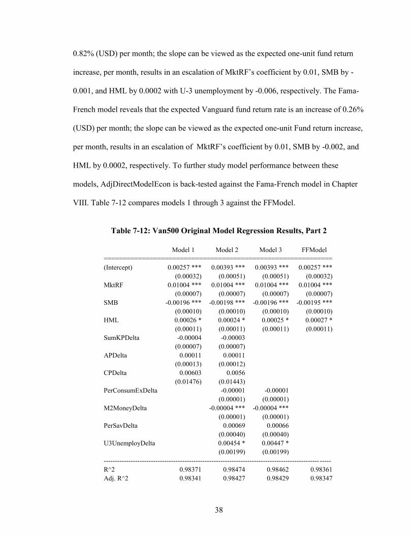
VIII. Table 7-12 compares models 1 through 3 against the FFModel.
Table 7-12: Van500 Original Model Regression Results, Part 2
Model 1 Model 2 Model 3 FFModel
============================================================
(Intercept) 0.00257 *** 0.00393 *** 0.00393 *** 0.00257 ***
(0.00032) (0.00051) (0.00051) (0.00032)
MktRF 0.01004 *** 0.01004 *** 0.01004 *** 0.01004 ***
(0.00007) (0.00007) (0.00007) (0.00007)
SMB -0.00196 *** -0.00198 *** -0.00196 *** -0.00195 ***
(0.00010) (0.00010) (0.00010) (0.00010)
HML 0.00026 * 0.00024 * 0.00025 * 0.00027 *
(0.00011) (0.00011) (0.00011) (0.00011)
SumKPDelta -0.00004 -0.00003
(0.00007) (0.00007)
APDelta 0.00011 0.00011
(0.00013) (0.00012)
CPDelta 0.00603 0.0056
(0.01476) (0.01443)
PerConsumExDelta -0.00001 -0.00001
(0.00001) (0.00001)
M2MoneyDelta -0.00004 *** -0.00004 ***
(0.00001) (0.00001)
PerSavDelta 0.00069 0.00066
(0.00040) (0.00040)
U3UnemployDelta 0.00454 * 0.00447 *
(0.00199) (0.00199)
------------------------------------------------------------------------------------------------ -----
R^2 0.98371 0.98474 0.98462 0.98361
Adj. R^2 0.98341 0.98427 0.98429 0.98347

39
The change in geomagnetic activity (i.e., SumKPDelta, APDelta, and CPDelta),
as shown in Model 1, has decreased model performance in RMSE, p-values, and Adj. R2.
Human economic behavior variables M2MoneyDelta (i.e., the change in money velocity)
and U3UnemployDelta (i.e., the change in unemployment) all have promising results and
statistically significant. Table 7-13 represents the adjusted version of Model 2 compared
to the FFModel.
Table 7-13: Van500 Adjusted Model 2 v. FFModel
AdjModel 2 FFModel
====================================
(Intercept) 0.00354 *** 0.00257 ***
(0.00043) (0.00032)
MktRF 0.01003 *** 0.01004 ***
(0.00007) (0.00007)
SMB -0.00199 *** -0.00195 ***
(0.00010) (0.00010)
HML 0.00026 * 0.00027 *
(0.00011) (0.00011)
M2MoneyDelta -0.00004 **
(0.00001)
U3UnemployDelta 0.00489 *
(0.00198)
-------------------------------------------------------------
R^2 0.98434 0.98361
Adj. R^2 0.9841 0.98347
Num. obs. 338 338
RMSE 0.00559 0.0057
====================================
*** p < 0.001, ** p < 0.01, * p < 0.05
Model performance of AdjModel 2 has shown an increase in Adj. R2 by 0.063%.
In addition, RMSE has decreased by 0.0011 which indicates stronger estimation
performance (and absolute fit) compared to the FFModel when the absolute change
(delta) in both Money Velocity and U-3 unemployment is used in the model. Severe
Num. obs. 338 338 338 338
RMSE 0.00571 0.00556 0.00556 0.0057
============================================================
*** p < 0.001, ** p < 0.01, * p < 0.05

40
multicollinearity does not exist with this particular model with variance inflation factors
at 1.10 (MktRF), 1.14 (SMB), 1.15 (HML), 1.027 (M2MoneyDelta), and 1.0031
(U3UnemployDelta). The intercept of AdjModel 2 suggests that the expected Vanguard
S&P 500 Fund return rate is 0.35% (USD) per month; the slope can be viewed as the
expected one-unit fund return increase, per month, results in an escalation of MktRF’s
coefficient by 0.01, SMB by -0.002, HML by 0.0003, and the change in money velocity
by -0.00004 with U-3 unemployment (delta) by 0.005, respectively. To further study the
model performance between these models, AdjDirectModelEcon is back-tested against
the Fama-French model in Chapter VIII. Table 7-14 compares models 4 to 6 against the
FFModel.
Table 7-14: Van500 Original Model Regression Results, Part 3
Model 4 Model 5 Model 6 FFModel
========================================================
(Intercept) 0.00940 * 0.00900 *** 0.00933 * 0.00257 ***
(0.00403) (0.00241) (0.00403) (0.00032)
SumKPDelta -0.00048 -0.00037
(0.00054) (0.00055)
APDelta -0.00037 -0.00051
(0.00097) (0.00098)
CPDelta 0.08572 0.06691
(0.11366) (0.11393)
PerConsumExDelta 0.00014 0.00014
(0.00008) (0.00008)
M2MoneyDelta -0.00016 -0.00016
(0.00009) (0.00009)
PerSavDelta 0.00325 0.00368
(0.00315) (0.00314)
U3UnemployDelta -0.01553 -0.01367
(0.01558) (0.01555)
MktRF 0.01004 ***
(0.00007)
SMB -0.00195 ***
(0.00010)
HML 0.00027 *
(0.00011)
----------------------------------------------------------------------------------------------- -

41
Models 4 to 6 do not contain any Fama-French factors (i.e., MktRF, SMB, and
HML). These models use absolute change (delta) in either geomagnetic activity, human
economic behavior, or both. Based on performance results, neither of these models would
be a candidate for backtesting against the FFModel. In addition, no statistical significance
was revealed in this scenario between each additional variable (aside from the Fama-
French factors) and the dependent variable. Table 7-15 includes results for models 7 to 9
against the Fama-French model.
Table 7-15: Van500 Original Model Regression Results, Part 4
R^2 0.03533 0.01072 0.02445 0.98361
Adj. R^2 0.01487 0.00184 0.01273 0.98347
Num. obs. 338 338 338 338
RMSE 0.04402 0.04431 0.04406 0.0057
========================================================
*** p < 0.001, ** p < 0.01, * p < 0.05
Model 7 Model 8 Model 9 FFModel
==================================================
(Intercept) 0.05952 0.01761 0.02433 0.00257 ***
(0.04347) (0.02590) (0.02393) (0.00032)
PerConsumEx -0.00001 -0.00001
(0.00001) (0.00001)
M2Money 0.00001 0.00001
(0.00001) (0.00001)
U3Unemploy 0.00107 0.00166
(0.00246) (0.00237)
PerSavRate -0.00165 -0.00168
(0.00276) (0.00276)
SumKp -0.00038 -0.00012
(0.00059) (0.00055)
Ap -0.00001 -0.00019
(0.00120) (0.00118)
Cp 0.0678 0.02516
(0.13340) (0.12917)
MktRF 0.01004 ***
(0.00007)
SMB -0.00195 ***
(0.00010)
HML 0.00027 *
(0.00011)
42
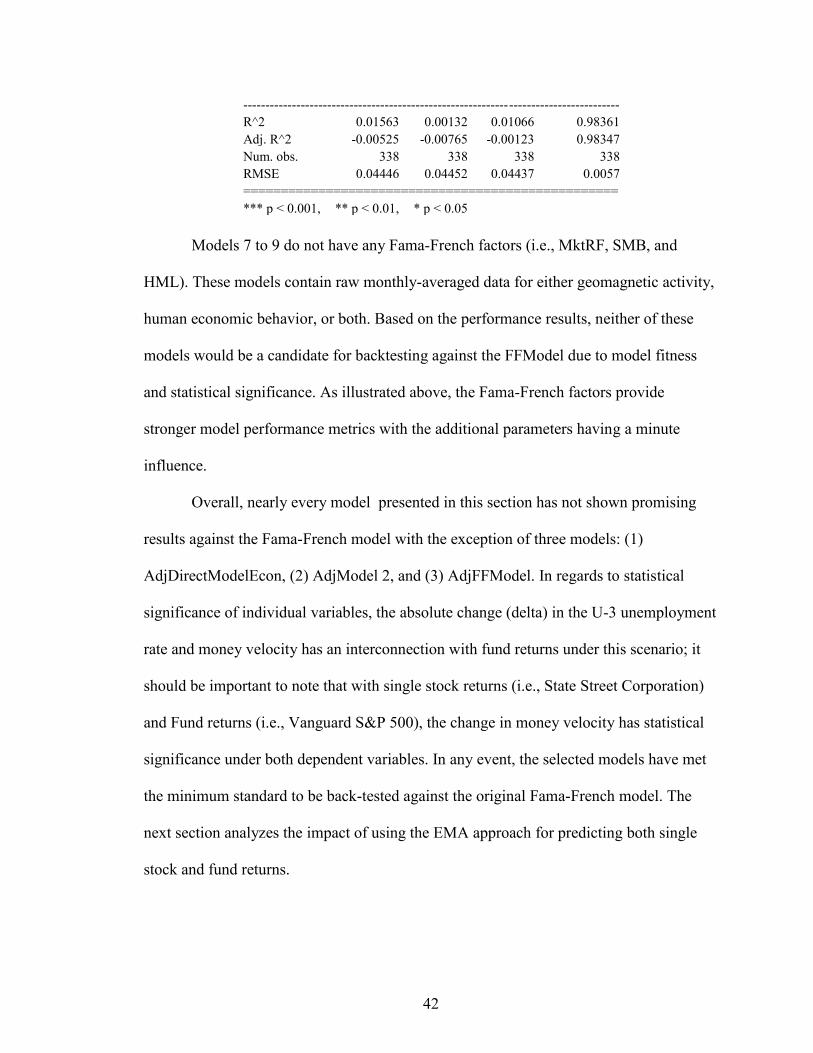
Models 7 to 9 do not have any Fama-French factors (i.e., MktRF, SMB, and
HML). These models contain raw monthly-averaged data for either geomagnetic activity,
human economic behavior, or both. Based on the performance results, neither of these
models would be a candidate for backtesting against the FFModel due to model fitness
and statistical significance. As illustrated above, the Fama-French factors provide
stronger model performance metrics with the additional parameters having a minute
influence.
Overall, nearly every model presented in this section has not shown promising
results against the Fama-French model with the exception of three models: (1)
AdjDirectModelEcon, (2) AdjModel 2, and (3) AdjFFModel. In regards to statistical
significance of individual variables, the absolute change (delta) in the U-3 unemployment
rate and money velocity has an interconnection with fund returns under this scenario; it
should be important to note that with single stock returns (i.e., State Street Corporation)
and Fund returns (i.e., Vanguard S&P 500), the change in money velocity has statistical
significance under both dependent variables. In any event, the selected models have met
the minimum standard to be back-tested against the original Fama-French model. The
next section analyzes the impact of using the EMA approach for predicting both single
stock and fund returns.
-------------------------------------------------------------------------------------
R^2 0.01563 0.00132 0.01066 0.98361
Adj. R^2 -0.00525 -0.00765 -0.00123 0.98347
Num. obs. 338 338 338 338
RMSE 0.04446 0.04452 0.04437 0.0057
==================================================
*** p < 0.001, ** p < 0.01, * p < 0.05

43
EMA Approach: State Street Corporation Stock Returns
In this section, the Exponential Moving Average (EMA) calculation is applied to
all geomagnetic and human economic behavior variables. The mean (µ) data ranges from
December 2004 to November 2009, or 60 monthly periods. EMA is calculated from
December 2009 to November 2014, or 60 monthly periods—this totals 120 monthly
periods for the entire EMA calculation per variable. The filtered data is then applied to
selected time-series regression equations without absolute delta (i.e., models 7, 8, and 9)
located in Chapter IV. After the time-series regression outputs have been calculated with
the selected data, the model’s parameters are later modified (if applicable) to meet the
cut-off p-value of any measurement over 5%. To meet this requirement, the focus of the
regression output includes the following: (i) Adj. R2, (ii) RMSE (root-mean-squared-
error), and (iii) p-values (0.1%, 1%, or 5%). A variance inflation factor (VIF) analysis
will typically occur after the model’s parameters have been adjusted (or removed). Table
7-16 includes the DirectModelEMA, where geomagnetic variables are included with the
Fama-French factors—and DirectModelEconEMA, which includes all variables from
DirectModelEMA, but with human economic behavior—these models are then compared
to the original Fama-French model (FFModel).

44
Table 7-16: STT EMA Approach, Part 1
DirectModelEMA DirectModelEconEMA FFModel
==========================================================
(Intercept) -145.83535 * -446.40157 -0.03378
(59.42577) (254.28985) (0.29873)
MktRF 0.49109 *** 0.51782 *** 0.51092 ***
(0.08590) (0.08977) (0.08534)
SMB -0.0117 -0.03624 -0.05085
(0.14966) (0.15563) (0.14276)
HML 0.41218 * 0.29543 0.34808 *
(0.16210) (0.17854) (0.15638)
SumKPEMA 3.02710 * 2.66491
(1.23583) (1.38704)
APEMA 18.87762 32.51185
(10.93672) (19.66680)
CPEMA -1061.32479 * -1286.97534 *
(476.66508) (606.47685)
PerConsumExEMA 0.05901
(0.04160)
PerSavRateEMA 1.63146
(3.48629)
U3UnemployEMA -1.96478
(1.99826)
M2MoneyEMA -0.03292
(0.02227)
---------------------------------------------------------------------------------------------------
R^2 0.58268 0.60854 0.53096
Adj. R^2 0.53544 0.52865 0.50583
Num. obs. 60 60 60
RMSE 2.08313 2.09828 2.14849
==========================================================
*** p < 0.001, ** p < 0.01, * p < 0.05
With the FFModel at an Adj. R2 of 50.58%, a RMSE of 2.1484, and an
insignificant p-value of Fama and French’s market parameter (SMB), a leaner
DirectModelEMA equation may prove more viable since the geomagnetic variable
(SumKPEMA) appears to have a statistical significance with its dependent variable. In
regards to DirectModelEconEMA, the model appears to not provide any significant
factors other than its inflated Adj. R2 and RMSE including insignificant p-values, with the
exception of Fama and French’s market parameter (MktRF). Below is a relationship test,

45
to determine if DirectModelEMA should be re-fitted, of the geomagnetic parameter
SumKPEMA with the dependent variable (i.e., STT).
Table 7-17: STT EMA Kp Index Relationship Test
Based on a p-value for SumKPEMA of 51.4%, this variable is insignificant and deflated
by other parameters in the DirectModelEMA equation. Table 7-18 below displays a
comparison of models 7, 8, and 9 to the FFModel:
Table 7-18: STT EMA Approach, Part 2
Model7EMA Model8EMA Model9EMA FFModel
===========================================================
(Intercept) -262.68058 -132.11973 17.09298 -0.03378
(358.02382) (87.03036) (187.22814) (0.29873)
PerConsumExEMA 0.03922 -0.00194
(0.05749) (0.03552)
PerSavRateEMA 5.83306 4.5926
(5.01775) (2.87692)
U3UnemployEMA -3.51136 -2.26238
(2.86517) (2.05875)
M2MoneyEMA -0.02315 -0.00042
(0.03069) (0.01976)
SumKPEMA 1.38665 2.62064
(1.96201) (1.79145)
APEMA 25.65702 19.95769
(27.99070) (15.91724)
CPEMA -902.60629 -981.66054
(881.36444) (697.82388)
MktRF 0.51092 ***
(0.08534)
===========================================
Residuals:
Min 1Q Median 3Q Max
-6.7003 -1.6085 0.2185 1.7968 7.3115
Coefficients:
Estimate Std. Error t value Pr(>|t|)
(Intercept) -1.12E+01 1.79E+01 -0.622 0.536
SumKPEMA 9.91E-02 1.51E-01 0.656 0.514
===========================================
*** p < 0.001, ** p < 0.01, * p < 0.05

46
SMB -0.05085
(0.14276)
HML 0.34808 *
(0.15638)
----------------------------------------------------------------------------------------------------
R^2 0.11598 0.0419 0.06518 0.53096
Adj. R^2 -0.00302 -0.00942 -0.00281 0.50583
Num. obs. 60 60 60 60
RMSE 3.0609 3.07066 3.06057 2.14849
===========================================================
*** p < 0.001, ** p < 0.01, * p < 0.05
Overall, the Exponential Moving Average (EMA) data filter approach for both
geomagnetic and human economic behavioral activity appears to not have meaningful
significance for predicting single stock returns by p-values, Adj. R2, and RSME. In the
end, the best performer for quantitative estimation, in this exercise, is the Fama-French
model (i.e., FFModel). The next section will use the same approach with the
Corporation’s stock returns, but at the fund level exposing the proposed variables to a
larger market environment.
EMA Approach: Vanguard S&P 500 Fund Returns
The reason for using Vanguard S&P 500 is because the Fama-French model
typically performs much stronger compared to the use of a single stock due to its
parameter construction. In this section, the Exponential Moving Average (EMA)
calculation is applied to all geomagnetic and human economic behavior variables. The
mean (µ) data ranges from December 2004 to November 2009, or 60 monthly periods.
EMA is calculated from December 2009 to November 2014, or 60 monthly periods—this
totals 120 monthly periods for the entire EMA calculation per variable. The filtered data
is then applied to selected time-series regression equations without absolute delta (i.e.,
models 7, 8, and 9) located in Chapter IV. After the time-series regression outputs have

47
been calculated with the selected data, the model’s parameters could be modified (if
applicable) to meet the cut-off p-value of any measurement over 5%. To meet this
requirement, the focus of the regression output includes the following: (i) Adj. R2, (ii)
RMSE (root-mean-squared-error), and (iii) p-values (0.1%, 1%, or 5%). A variance
inflation factor (VIF) analysis will typically occur after the model’s parameters have been
adjusted (or removed). Table 7-19 contains the DirectModelEMA, where geomagnetic
variables are included with the Fama-French factors—and DirectModelEconEMA, which
uses all variables from DirectModelEMA, but with human economic behavior—these
models are then compared to the original Fama-French model (FFModel) for Vanguard
S&P 500 Fund returns.
Table 7-19: Van500 EMA Approach, Part 1
DirectModelEMA DirectModelEconEMA FFModel
===========================================================
(Intercept) 0.01426 -0.2371 -0.0001
(0.05186) (0.21621) (0.00025)
MktRF 0.00990 *** 0.00992 *** 0.00993 ***
(0.00007) (0.00008) (0.00007)
SMB -0.00133 *** -0.00135 *** -0.00140 ***
(0.00013) (0.00013) (0.00012)
HML 0.00012 0.00017 0.00005
(0.00014) (0.00015) (0.00013)
SumKPEMA 0.00005 0.00106
(0.00108) (0.00118)
APEMA -0.00677 0.01156
(0.00954) (0.01672)
CPEMA 0.0923 -0.45197
(0.41594) (0.51565)
PerConsumExEMA 0.00003
(0.00004)
PerSavRateEMA -0.00666 *
(0.00296)
U3UnemployEMA 0.00272
(0.00170)
M2MoneyEMA -0.00001
(0.00002)
----------------------------------------------------------------------------------------------------
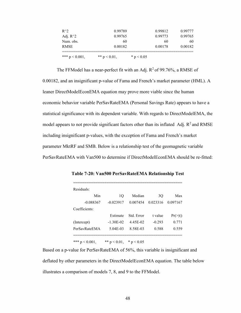
48
The FFModel has a near-perfect fit with an Adj. R2 of 99.76%, a RMSE of
0.00182, and an insignificant p-value of Fama and French’s market parameter (HML). A
leaner DirectModelEconEMA equation may prove more viable since the human
economic behavior variable PerSavRateEMA (Personal Savings Rate) appears to have a
statistical significance with its dependent variable. With regards to DirectModelEMA, the
model appears to not provide significant factors other than its inflated Adj. R2 and RMSE
including insignificant p-values, with the exception of Fama and French’s market
parameter MktRF and SMB. Below is a relationship test of the geomagnetic variable
PerSavRateEMA with Van500 to determine if DirectModelEconEMA should be re-fitted:
Table 7-20: Van500 PerSavRateEMA Relationship Test
Based on a p-value for PerSavRateEMA of 56%, this variable is insignificant and
deflated by other parameters in the DirectModelEconEMA equation. The table below
illustrates a comparison of models 7, 8, and 9 to the FFModel.
R^2 0.99789 0.99812 0.99777
Adj. R^2 0.99765 0.99773 0.99765
Num. obs. 60 60 60
RMSE 0.00182 0.00178 0.00182
===========================================================
*** p < 0.001, ** p < 0.01, * p < 0.05
=================================================
Residuals:
Min 1Q Median 3Q Max
-0.088367 -0.023917 0.007454 0.023316 0.097167
Coefficients:
Estimate Std. Error t value Pr(>|t|)
(Intercept) -1.30E-02 4.45E-02 -0.293 0.771
PerSavRateEMA 5.04E-03 8.58E-03 0.588 0.559
=================================================
*** p < 0.001, ** p < 0.01, * p < 0.05
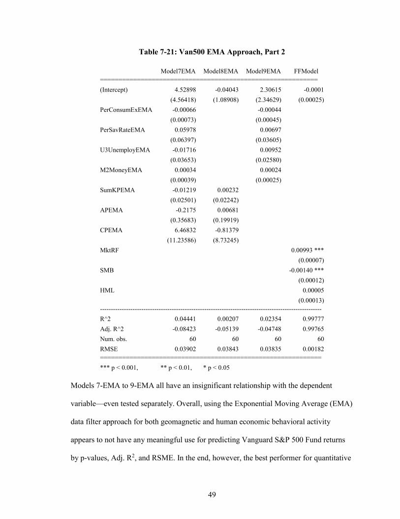
49
Table 7-21: Van500 EMA Approach, Part 2
Model7EMA Model8EMA Model9EMA FFModel
===========================================================
(Intercept) 4.52898 -0.04043 2.30615 -0.0001
(4.56418) (1.08908) (2.34629) (0.00025)
PerConsumExEMA -0.00066 -0.00044
(0.00073) (0.00045)
PerSavRateEMA 0.05978 0.00697
(0.06397) (0.03605)
U3UnemployEMA -0.01716 0.00952
(0.03653) (0.02580)
M2MoneyEMA 0.00034 0.00024
(0.00039) (0.00025)
SumKPEMA -0.01219 0.00232
(0.02501) (0.02242)
APEMA -0.2175 0.00681
(0.35683) (0.19919)
CPEMA 6.46832 -0.81379
(11.23586) (8.73245)
MktRF 0.00993 ***
(0.00007)
SMB -0.00140 ***
(0.00012)
HML 0.00005
(0.00013)
------------------------------------------------------------------------------------------------------
R^2 0.04441 0.00207 0.02354 0.99777
Adj. R^2 -0.08423 -0.05139 -0.04748 0.99765
Num. obs. 60 60 60 60
RMSE 0.03902 0.03843 0.03835 0.00182
============================================================
*** p < 0.001, ** p < 0.01, * p < 0.05
Models 7-EMA to 9-EMA all have an insignificant relationship with the dependent
variable—even tested separately. Overall, using the Exponential Moving Average (EMA)
data filter approach for both geomagnetic and human economic behavioral activity
appears to not have any meaningful use for predicting Vanguard S&P 500 Fund returns
by p-values, Adj. R2, and RSME. In the end, however, the best performer for quantitative

50
estimation in this exercise is the Fama-French model (i.e., FFModel). The last section
concludes the analysis for Chapter VII.
Concluding Analysis for Chapter VII
Chapter VII analyzed how geomagnetic and human economic behavioral
parameters could impact fund and stock returns against the Fama-French model. This
Chapter used the original approach, which includes regression equations in Chapter IV
and the EMA approach located in Chapter V. The original approach in State Street
Corporation’s stock returns concluded that the absolute change (delta) in the velocity of
money (M2MoneyDelta) is statistically significant at 2.1%; by adding that parameter to
the original Fama-French model (i.e., AdjFFModel), it slightly improved model
performance compared to the original despite the p-value being inflated above the 5%
significance level. Model output for the Vanguard S&P 500 Fund experienced promising
results with AdjDirectModelEcon and AdjModel 2. For AdjDirectModelEcon, the U-3
unemployment rate has statistical significance at p < 0.001 with improved Adj. R2 and
RMSE when compared to the original Fama-French model. AdjModel 2 revealed that not
only the absolute change in the U-3 unemployment rate has statistical significance with
fund returns, but also the velocity of money at p < 0.001 and p < 0.01, respectively; the
overall model performance revealed a slight improvement in both Adj. R2 and RMSE
when compared to the original Fama-French model. Since these models have challenging
metrics against the benchmark, they are back-tested in Chapter VIII. The tables below
represent short-listed models for this Chapter.

51
Table 7-22: STT Short-Listed Models for Chapter VII
AdjFFModel FFModel
=================================
(Intercept) 0.11346 -0.06705
(0.18044) (0.13014)
MktRF 0.36421 *** 0.36832 ***
(0.02975) (0.02967)
SMB -0.09746 * -0.09350 *
(0.04238) (0.04236)
HML 0.20425 *** 0.21147 ***
(0.04633) (0.04613)
M2MoneyDelta -0.00667
(0.00463)
--------------------------------------------------------
R^2 0.33065 0.32647
Adj. R^2 0.32261 0.32042
Num. obs. 338 338
RMSE 2.34991 2.3537
=================================
*** p < 0.001, ** p < 0.01, * p < 0.05
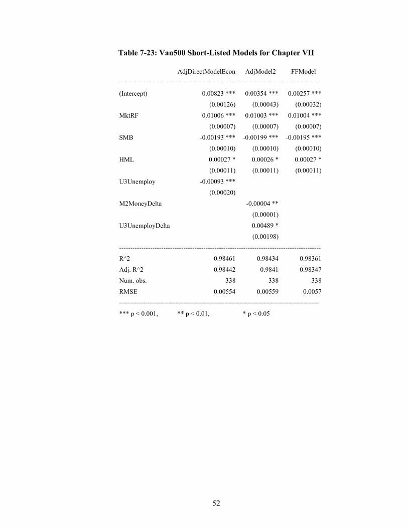
52
Table 7-23: Van500 Short-Listed Models for Chapter VII
AdjDirectModelEcon AdjModel2 FFModel
=====================================================
(Intercept) 0.00823 *** 0.00354 *** 0.00257 ***
(0.00126) (0.00043) (0.00032)
MktRF 0.01006 *** 0.01003 *** 0.01004 ***
(0.00007) (0.00007) (0.00007)
SMB -0.00193 *** -0.00199 *** -0.00195 ***
(0.00010) (0.00010) (0.00010)
HML 0.00027 * 0.00026 * 0.00027 *
(0.00011) (0.00011) (0.00011)
U3Unemploy -0.00093 ***
(0.00020)
M2MoneyDelta -0.00004 **
(0.00001)
U3UnemployDelta 0.00489 *
(0.00198)
-------------------------------------------------------------------------------------------
R^2 0.98461 0.98434 0.98361
Adj. R^2 0.98442 0.9841 0.98347
Num. obs. 338 338 338
RMSE 0.00554 0.00559 0.0057
=====================================================
*** p < 0.001, ** p < 0.01, * p < 0.05
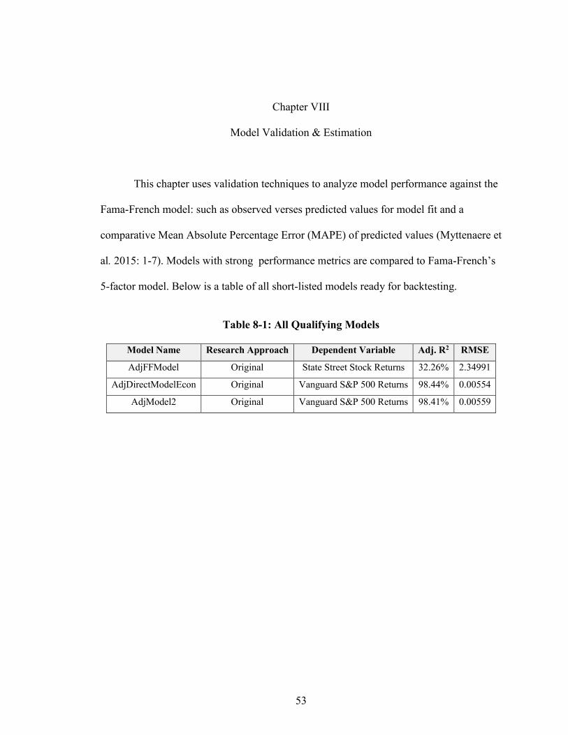
53
Chapter VIII
Model Validation & Estimation
This chapter uses validation techniques to analyze model performance against the
Fama-French model: such as observed verses predicted values for model fit and a
comparative Mean Absolute Percentage Error (MAPE) of predicted values (Myttenaere et
al. 2015: 1-7). Models with strong performance metrics are compared to Fama-French’s
5-factor model. Below is a table of all short-listed models ready for backtesting.
Table 8-1: All Qualifying Models
Model Name Research Approach Dependent Variable Adj. R2 RMSE
AdjFFModel Original State Street Stock Returns 32.26% 2.34991
AdjDirectModelEcon Original Vanguard S&P 500 Returns 98.44% 0.00554
AdjModel2 Original Vanguard S&P 500 Returns 98.41% 0.00559

54
Model Fitness Test: STT Observed verses Predicted Values
This section will use the selected models above and predict values, compare those
predicted values to observed (actual) values, then analyze those quantities to the
corresponding Fama-French model for State Street Corporation’s stock returns. This
section uses 338 known periods (months) in this exercise for both dependent and
independent variables using returns. For a model(s) to meet or exceed performance
metrics against the benchmark, their average predication accuracy, calculated by the
Mean Absolute Percentage Error (MAPE), has to outperform the Fama-French model;
any model with a percentage error over 100 is absolutely inaccurate. Figure 8-1 compares
observed (actual) stock returns to the model’s predicted results (AdjFFModel) including
the Fama-French model (FFModel).
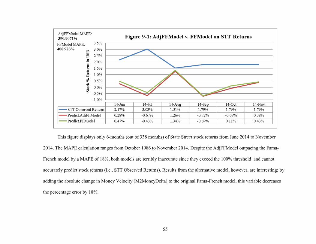
55
This figure displays only 6-months (out of 338 months) of State Street stock returns from June 2014 to November
2014. The MAPE calculation ranges from October 1986 to November 2014. Despite the AdjFFModel outpacing the Fama-
French model by a MAPE of 18%, both models are terribly inaccurate since they exceed the 100% threshold and cannot
accurately predict stock returns (i.e., STT Observed Returns). Results from the alternative model, however, are interesting; by
adding the absolute change in Money Velocity (M2MoneyDelta) to the original Fama-French model, this variable decreases
the percentage error by 18%.
56
Model Fitness Test: Vanguard Observed verses Predicted Values
This section uses selected models noted in this Chapter and predict values,
compare those predicted values to observed (actual) values, then analyze those predicted
quantities to the corresponding Fama-French model for the Vanguard S&P 500 Fund
returns—the fund represents 75% of the U.S stock market. This section uses 338 known
periods (months) in this exercise for both the dependent and independent variable using
returns. For a model(s) to meet or exceed expectations of model performance, their
average predication accuracy, calculated by the Mean Absolute Percentage Error
(MAPE), has to outperform the Fama-French model. Any model with a percentage error
over 100 is absolutely inaccurate. Figure 8-2 compares observed (actual) fund returns to
the models’ predicted results (i.e., AdjDirectModelEcon and AdjModel2) including the
Fama-French model (FFModel).

57
For the Vanguard S&P 500 Fund, the table displays only 6-months (out of 338 months) of percent returns, in USD (i.e.,
United States Dollars), from June 2014 to November 2014. The MAPE calculation ranges from November 1986 to November
2014. All models presented in this table has less than a 25% historical percentage error. AdjModel2, in this case, has the best
performance metrics—the equation incorporates all Fama-French factors, but with added variables: such as the absolute
change in both money velocity and U-3 unemployment. These added variables reduce the Fama-French forecasting error by
2.753% on a historical basis. AdjDirectModelEcon’s performance is slightly worse than AdjModel2 with only U-3
unemployment and Fama-French factors used.

58
Robustness Analysis on Modeled Vanguard Returns: 2008-2009 Financial Crisis
During the 2008-2009 Financial Crisis, all models have performed exceptionally
well compared to actual percent returns (i.e., Van500 Returns). As noted earlier,
historically, the alternative model (i.e., AdjModel2) had a mean absolute percentage error
of 2.753% less than the Fama-French model. Between September to November 2008,
AdjModel2 was slightly closer to actual returns by an average difference of 0.06%
compared to the Fama-French model at 0.12%. The alternative model does have stronger
performance metrics compared to the Fama-French model, but the results are so close
that some scholars may warrant this comparison immaterial. If these models were used on
actual portfolios, however, fund managers (or market participants) would choose the best
overall model by historical performance if it can increase their bottom-line. The
alternative model contains all Fama-French factors, plus the absolute change in both U-3
unemployment and velocity of money equating to a 5-factor model.
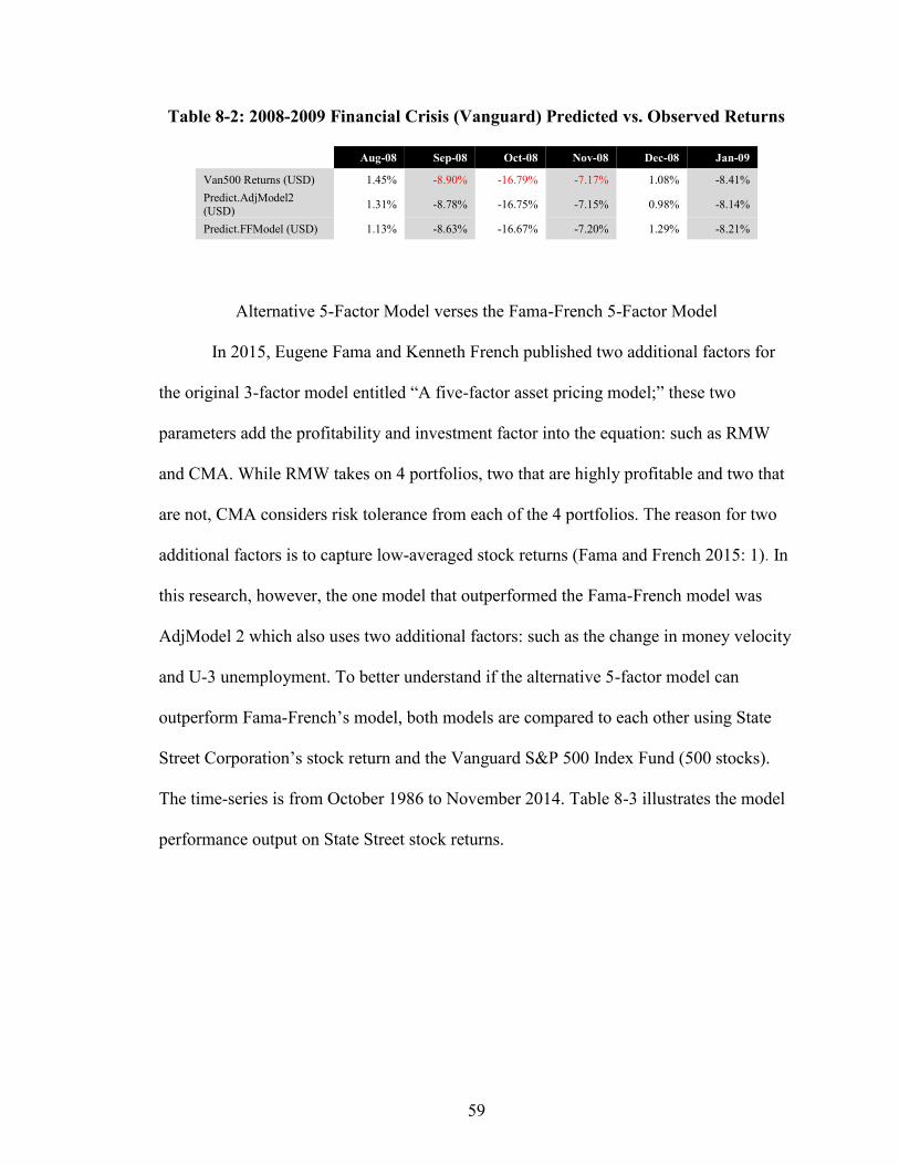
59
Table 8-2: 2008-2009 Financial Crisis (Vanguard) Predicted vs. Observed Returns
Aug-08 Sep-08 Oct-08 Nov-08 Dec-08 Jan-09
Van500 Returns (USD) 1.45% -8.90% -16.79% -7.17% 1.08% -8.41%
Predict.AdjModel2 (USD)
1.31% -8.78% -16.75% -7.15% 0.98% -8.14%
Predict.FFModel (USD) 1.13% -8.63% -16.67% -7.20% 1.29% -8.21%
Alternative 5-Factor Model verses the Fama-French 5-Factor Model
In 2015, Eugene Fama and Kenneth French published two additional factors for
the original 3-factor model entitled “A five-factor asset pricing model;” these two
parameters add the profitability and investment factor into the equation: such as RMW
and CMA. While RMW takes on 4 portfolios, two that are highly profitable and two that
are not, CMA considers risk tolerance from each of the 4 portfolios. The reason for two
additional factors is to capture low-averaged stock returns (Fama and French 2015: 1). In
this research, however, the one model that outperformed the Fama-French model was
AdjModel 2 which also uses two additional factors: such as the change in money velocity
and U-3 unemployment. To better understand if the alternative 5-factor model can
outperform Fama-French’s model, both models are compared to each other using State
Street Corporation’s stock return and the Vanguard S&P 500 Index Fund (500 stocks).
The time-series is from October 1986 to November 2014. Table 8-3 illustrates the model
performance output on State Street stock returns.

60
Table 8-3: Alternative 5-Factor v. Fama-French 5-Factor on STT Returns
The intercept of AdjModel2 suggests that the expected State Street stock return
rate is 12% (USD) per month; the slope can be viewed as the expected one-unit stock
return increase, per month, results in an escalation of MktRF’s coefficient by 0.366, SMB
by -0.095, HML by 0.20, M2MoneyDelta by -0.006, and U3UnemployDelta by 0.540,
respectively. For FFModel5, the model’s intercept suggests that the expected State Street
stock return rate is 2.1% (USD) per month; the slope can be viewed as the expected one-
unit stock return increase, per month, results in an escalation of MktRF’s coefficient by
0.34, SMB by -0.169, HML by 0.239, RMW by -0.20, and CMA by 0.015, respectively.
Lastly, FFModel’s output metrics resulted in an intercept that suggests expected State
AdjModel2 FFModel5 FFModel
==============================================
(Intercept) 0.12003 0.02099 -0.06705
(0.18088) (0.13438) (0.13014)
MktRF 0.36613 *** 0.34002 *** 0.36832 ***
(0.02993) (0.03293) (0.02967)
SMB -0.09938 * -0.16948 *** -0.09350 *
(0.04252) (0.04736) (0.04236)
HML 0.20703 *** 0.23944 *** 0.21147 ***
(0.04656) (0.06127) (0.04613)
M2MoneyDelta -0.00692
(0.00465)
U3UnemployDelta 0.54042
(0.83120)
RMW -0.20639 ***
(0.06164)
CMA 0.01521
(0.08759)
------------------------------------------------------------------------------
R^2 0.3315 0.34925 0.32647
Adj. R^2 0.32143 0.33944 0.32042
Num. obs. 338 338 338
RMSE 2.35195 2.32052 2.3537
==============================================
*** p < 0.001, ** p < 0.01, * p < 0.05
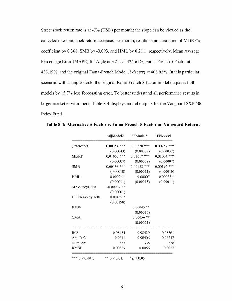
61
Street stock return rate is at -7% (USD) per month; the slope can be viewed as the
expected one-unit stock return decrease, per month, results in an escalation of MktRF’s
coefficient by 0.368, SMB by -0.093, and HML by 0.211, respectively. Mean Average
Percentage Error (MAPE) for AdjModel2 is at 424.61%, Fama-French 5 Factor at
433.19%, and the original Fama-French Model (3-factor) at 408.92%. In this particular
scenario, with a single stock, the original Fama-French 3-factor model outpaces both
models by 15.7% less forecasting error. To better understand all performance results in
larger market environment, Table 8-4 displays model outputs for the Vanguard S&P 500
Index Fund.
Table 8-4: Alternative 5-Factor v. Fama-French 5-Factor on Vanguard Returns
AdjModel2 FFModel5 FFModel
===============================================
(Intercept) 0.00354 *** 0.00220 *** 0.00257 ***
(0.00043) (0.00032) (0.00032)
MktRF 0.01003 *** 0.01017 *** 0.01004 ***
(0.00007) (0.00008) (0.00007)
SMB -0.00199 *** -0.00182 *** -0.00195 ***
(0.00010) (0.00011) (0.00010)
HML 0.00026 * -0.00005 0.00027 *
(0.00011) (0.00015) (0.00011)
M2MoneyDelta -0.00004 **
(0.00001)
U3UnemployDelta 0.00489 *
(0.00198)
RMW 0.00045 **
(0.00015)
CMA 0.00056 **
(0.00021)
--------------------------------------------------------------------------------
R^2 0.98434 0.98429 0.98361
Adj. R^2 0.9841 0.98406 0.98347
Num. obs. 338 338 338
RMSE 0.00559 0.0056 0.0057
===============================================
*** p < 0.001, ** p < 0.01, * p < 0.05

62
The intercept of AdjModel2 suggests that the expected Vanguard S&P 500 Fund
return rate is 0.35% (USD) per month; the slope can be viewed as the expected one-unit
fund return increase, per month, results in an escalation of MktRF’s coefficient by 0.01,
SMB by -0.0019, HML by 0.00026, M2MoneyDelta by -0.00004, and U3UnemployDelta
by 0.0048, respectively. For FFModel5, the model’s intercept suggests that the expected
Fund return rate is 0.22% (USD) per month; the slope can be viewed as the expected one-
unit stock return increase, per month, results in an escalation of MktRF’s coefficient by
0.01, SMB by -0.182, HML by -0.00005, RMW by 0.00045, and CMA by 0.00056,
respectively. Lastly, FFModel’s output metrics resulted in an intercept that suggests
expected State Street stock return rate is at 0.257% (USD) per month; the slope can be
viewed as the expected one-unit stock return increase, per month, results in an escalation
of MktRF’s coefficient by 0.01, SMB by -0.0019, and HML by 0.00027, respectively. In
terms of MAPE, the AdjModel2 yields a 21.83% forecasting error, FFModel5 at 24.64%,
and the FFModel at 24.6%. Out of all the models, the alternative 5-factor construction
outpaces all Fama-French results, in this exercise, by at least 2.753% in forecasting error.
The next section concludes this chapter.
Concluding Analysis for Chapter VIII
This chapter back-tested selected models against both the Fama-French 3 and 5-
Factor model. With actual verses predicted values using State Street stock returns, the
alternative model (i.e., AdjFFModel) outperformed the Fama-French 3-factor model by
MAPE at 390.90% versus the FFModel at 408.923%.Vanguard S&P Index Fund’s top
performer in quantitative estimation, on returns, is AdjModel2 with proven metrics that

63
outpaces the Fama-French 3-Factor model by nearly 3% less in historical forecasting
error.
In the Fama-French 5 factor model comparison, AdjModel 2 had more forecasting
error compared to the 3-factor model, but less against the 5-factor equation for single
stock returns (i.e., State Street Corporation). In terms of larger market exposure (i.e.,
Vanguard S&P 500 Index Fund), AdjModel 2 captures less forecasting error compared to
both Fama-French models.
Overall, the model with best overall fit, the least mean absolute percentage error,
and able to recognize severe market fluctuations against the Fama-French model is
AdjModel2. Although, in most cases, equations containing human economic behavior has
stronger model performance metrics compared to geomagnetic parameters, the change in
human behavioral activity defined by unemployment and money velocity, in combination
with three Fama-French factors, has the strongest impact in quantitative estimation. Next,
Chapter IX will conclude the entire analysis for this research.
64
Chapter IX
Research Conclusion
This research attempted to shed light on natural phenomena and human economic
behavioral impact in quantitative estimation using the Fama-French 3-factor model as a
benchmark. Chapter VII analyzed how all three methodological approaches could impact
quantitative estimation of equity and fund returns. Chapter VIII validated, estimated, and
compared short-listed models in previous chapters to Fama-French’s three and five factor
model. Appendix B discussed modeling results from transformed data. Appendix C
analyzed causality between geomagnetic indices and human economic behavior.
Appendix D and E revealed correlation results for all variables used in the research. The
purpose of this analysis is to answer two questions listed below:
1. Although research has revealed the potential interconnection of geomagnetic
activity with market behavior, could this natural phenomena actually increase the
prediction power of quantitative models?
2. What about the human behavioral element—does that play a role in econometric
modeling?
In addition to the questions above, this research hypothesized that the Earth’s magnetic
field and human economic behavior might play a small role with improving quantifiable
estimated outputs. Moreover, it was also hypothesized that magnetic activity could have a
direct impact on the defined human economic behavioral variables. In essence, some
initial claims are true for the proposed research questions. To answer question one,

65
geomagnetic activity does not have a strong impact in improving quantitative estimation
on returns, as revealed earlier for both a single stock and the top 500 combined equity
shares traded on the U.S. stock market. After accounting for data transformations in the
proposed modeling approaches, performance results were also insignificant against the
Fama-French Model. In addition, the EMA approach for equity and fund returns did not
reveal anything significant enough to improve or outpace the benchmark.
For question two, variables defined as human economic behavioral activity does
have a role to play in the Fama-French modeling approach. The change in the money
velocity and U-3 unemployment has statistical significance with returns under the
original approach for the Vanguard S&P 500 Fund; State Street stock returns, however,
only has a relationship with money velocity and not U-3 unemployment. So, since a few
human economic behavioral variables are decent predictors of returns, what about
causality? Is there any evidence suggesting that geomagnetic behavior might influence
human economic outcomes?
In Appendix C, this research analyzed whether causality might exist between
these two groups of data: (a) geomagnetic indices and (b) human economic behavior.
Unfortunately, the Granger test demonstrated that economic and geomagnetic data does
not contain enough information to forecast each other—in essence, there is an
insignificant direct or indirect connection among these parameters—this defeats the
research’s second null hypothesis suggesting that it does.
On the performance front, the only model worthy of mention is AdjModel2. This
model was tested against both the 3-Factor and 5-Factor model. In all cases except one,
the alternative 5-factor model outpaced Fama and French’s approach by a mean absolute

66
percentage error of roughly 3% less than the benchmark. In both a large and small
market environment, this model does have the potential to recognize swings in behavior
more accurately than the benchmark. Although this research area still needs maturing,
Eugene Fama and Kenneth French should consider environmental influences, such as
human economic behavior, legitimate factors to better estimate returns. In this research,
the evidence is clear that practitioners and academics should look outside their narrow
boarders for other significant factors that might influence research and investment
outcomes.
In conclusion, the first null hypothesis is considered half true: human economic
behavior does play, to some degree, a role in quantitative estimation on returns while
geomagnetic activity does not have strong enough influence in this research approach.
Although this study only scrapes the surface of answering the unknown, there are now
potential research gaps with additional asset classes: such as real estate, commodities,
fixed income, foreign exchange, and other investment vehicles. Among these asset
classes, regions and industries participating in any market should also be researched. In
artificial intelligence and machine learning for the financial industry, practitioners should
explore how this data might impact predicted outcomes due to the results in this research.
Lastly, although human economic behavior revealed some influence in this controlled
mathematical study with two dependent variables under one asset class, opportunities for
new research possibilities exist and should be sought-out for most academic disciplines
and practitioners.

67
Appendix A
Experiential Modeling with Adjusted Closed Prices
Chapter VII used fund and stock returns as the dependent variable. The original
Fama-French equation calls for returns, not adjusted closed prices. In this Appendix,
however, the dependent variable is changed to non-stationary adjusted closed prices. The
rationale for a dependent variable change is to analyze any impact of geomagnetic and
human economic behavior on temporal trends in price fluctuations. This chapter uses
both the original approach illustrated on Chapter IV and EMA filtered data for both asset
prices. In regards to the original approach, the monthly time-series ranges from October
1986 to November 2014. The data range derived from the EMA approach is from
December 2004 to November 2009, or 60 monthly periods; EMA is calculated from
December 2009 to November 2014, or 60 monthly periods. For variable elimination, the
focus of the regression output will include the following: (i) Adj. R2, (ii) RMSE (root-
mean-squared-error), and (iii) p-values (0.1%, 1%, or 5%). A variance inflation factor
(VIF) analysis will typically occur after the model’s parameters have been adjusted (or
removed). Robustness analysis during the 2008-2009 Financial Crisis, in addition to a
model fitness test of observed verses predict values, is displayed in this appendix. Models
are denoted with a “P” to signify that the dependent variable represents adjusted closed
prices and not returns. Section A-1 analyzes final regression results for State Street
Corporation’s closed adjusted prices.

68
Section A-1: State Street Corporation Stock Prices
Table A-1.1: STT Model Regression Results
AdjDir..EconP AdjDir..EconP2 AdjDir..EconP3
==================================================
(Intercept) 5.93391 10.20130 *** -26.60961 ***
(3.54589) (2.54811) (3.03669)
SumKp 0.01657
(0.00961)
PerConsumEx 0.00581 *** 0.00562 *** 0.00716 ***
(0.00021) (0.00018) (0.00022)
PerSavRate -3.61286 *** -3.64793 ***
(0.27851) (0.27858)
DSavKp 0.02982 *
(0.01166)
-------------------------------------------------------------------------------------
R^2 0.87265 0.87152 0.80947
Adj. R^2 0.87151 0.87075 0.80833
Num. obs. 338 338 338
RMSE 7.47867 7.5007 9.13397
==================================================
*** p < 0.001, ** p < 0.01, * p < 0.05
Variance inflation factors for the AdjDirectModelEconP equation are at 1.49
(SumKP), 1.946 (PerConsumEx), and 1.40 (PerSavRate)—variables, such as the
PerConsumEx and PerSavRate, are higher than expected inflation factors causing the
SumKP’s p-value to be inflated. With the SumKP removed, AdjDirectModelEconP2’s
variance inflation factors are at 1.393 (PerConsumEx) and 1.393 (PerSavRate). To further
enhance the geomagnetic Kp Index, an independent variable difference calculation was
conducted between PerSavRate and SumKp with a new variable entitled “DSavKp”—
using this variable along with PerConsumEx, the AdjDirectModelEconP3 equation
decreased the p-value of the Kp Index below 5%, but greater than 1% when modeled with
human economic behavior—this model, however, suffers from a lowered Adjusted R2

69
and a higher RMSE; variance inflation actors are at 1.45 for both PerConsumEx and
DSavKp. All alternative models have an Adj. R2 of at least 80%.
The intercept of AdjDirectModelEconP suggests that the expected State Street
stock return rate is $5.93 (USD) per month; the slope can be viewed as the expected one-
unit increase of the stock return, per month, results in an escalation of SumKp’s
coefficient by 0.02, personal consumption expenditure (PerConsumEx) by 0.00581, and
personal savings rate (PerSavRate) by -3.612, respectively. Regarding
AdjDirectModelEconP2, the intercept suggests that the expected State Street stock return
rate is $10.20 (USD) per month; the slope can be viewed as the expected one-unit
increase of the stock return, per month, results in an escalation of personal consumption
expenditure’s coefficient (PerConsumEx) by 0.00562 and personal savings rate
(PerSavRate) by -3.64, respectively. Lastly, AdjDirectModelEconP3’s intercept
concludes that the expected State Street stock return rate, per share, is -$26.61 (USD) per
month; the slope can be viewed as the expected one-unit decrease of the stock return, per
month, results in an escalation of personal consumption expenditure’s coefficient
(PerConsumEx) by 0.00716 and the difference between personal savings rate and the KP
index (DSavKp) by 0.02982, respectively. Section A-2 analyzes regression results for the
Vanguard S&P 500 Fund.
Section A-2: Vanguard S&P 500 Fund Prices
Table A-2.1: Van500 Regression Results
AltRefitMod1 AltRefitMod2 AdjDir..EconP3
==================================================
(Intercept) -70.28248 ** -76.81129 *** 41.10021 ***
(24.84088) (21.64883) (3.45093)
PerSavRate -2.24614 ** -2.08346 **
(0.69629) (0.69371)
M2MoneyEMA 0.03500 *** 0.03565 ***

70
(0.00095) (0.00100)
APEMA -11.99171 **
(3.45945)
CPEMA -272.32490 ***
(72.87854)
C9 -0.88783
(0.62934)
M2Money 0.01731 ***
(0.00030)
U3Unemploy -11.12161 ***
(0.43383)
-------------------------------------------------------------------------------------
R^2 0.96408 0.96508 0.93283
Adj. R^2 0.96216 0.96321 0.93222
Num. obs. 60 60 338
RMSE 5.57431 5.49619 10.68677
==================================================
*** p < 0.001, ** p < 0.01, * p < 0.05
Variance inflation factors, for AltRefitMod1, are at 1.04 (PerSavRate), 1.14
(M2MoneyEMA), and 1.14(APEMA). For AltRefitMod2, inflation factors are now at
1.06 (PerSavRate), 1.30 (M2MoneyEMA), and 1.31(CPEMA). Using the Cp
geomagnetic index, compared to the AP Index, the variable slightly inflates the variance.
The intercept of AltRefitMod1 suggests that the expected Vanguard S&P 500 Index Fund
return rate is -$70.28 (USD) per month; the slope can be viewed as the expected one-unit
stock return decrease, per month, results in a de-escalation of personal savings rate’s
coefficient by -2.24, money velocity by 0.035, and APEMA by -11.991, respectively. For
AltRefitMod2, the model’s intercept suggests that the expected Vanguard S&P 500 Index
Fund rate is $-76.81 (USD) per month; the slope can be viewed as the expected one-unit
fund return decrease, per month, results in a de-escalation of personal savings rate’s
coefficient by -2.08, M2MoneyEMA by 0.035, and CPEMA by -272.32, respectively.
The Fama-French model is still expected to outpace both alternative models, but
regardless of those metrics, these models will be back-tested. Under AdjDirectModel-

71
EconP3, the inflation factors are at 1.43 (C9), 1.65 (M2Money), and 1.25(U3Unemploy).
The intercept of AdjDirectModelEconP3 suggests that the expected Vanguard S&P 500
Index Fund return rate is $41.10 (USD) per month; the slope can be viewed as the
expected one-unit fund return increase, per month, results in an escalation of the velocity
of money’s (M2Money) coefficient by 0.0173, unemployment (U3Unemploy) by -
11.121, and the geomagnetic C9 Index (C9) by -0.887, respectively. Section A-3 analyzes
model fitness and robustness for single stock prices.
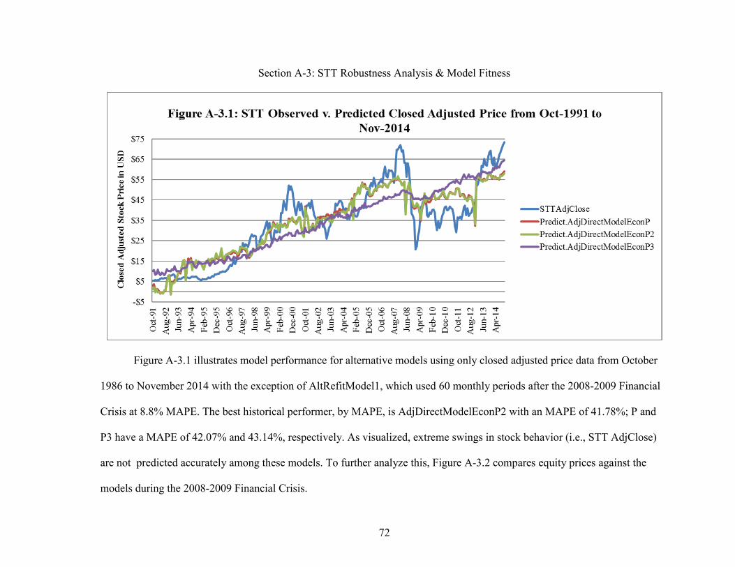
72
Section A-3: STT Robustness Analysis & Model Fitness
Figure A-3.1 illustrates model performance for alternative models using only closed adjusted price data from October
1986 to November 2014 with the exception of AltRefitModel1, which used 60 monthly periods after the 2008-2009 Financial
Crisis at 8.8% MAPE. The best historical performer, by MAPE, is AdjDirectModelEconP2 with an MAPE of 41.78%; P and
P3 have a MAPE of 42.07% and 43.14%, respectively. As visualized, extreme swings in stock behavior (i.e., STT AdjClose)
are not predicted accurately among these models. To further analyze this, Figure A-3.2 compares equity prices against the
models during the 2008-2009 Financial Crisis.
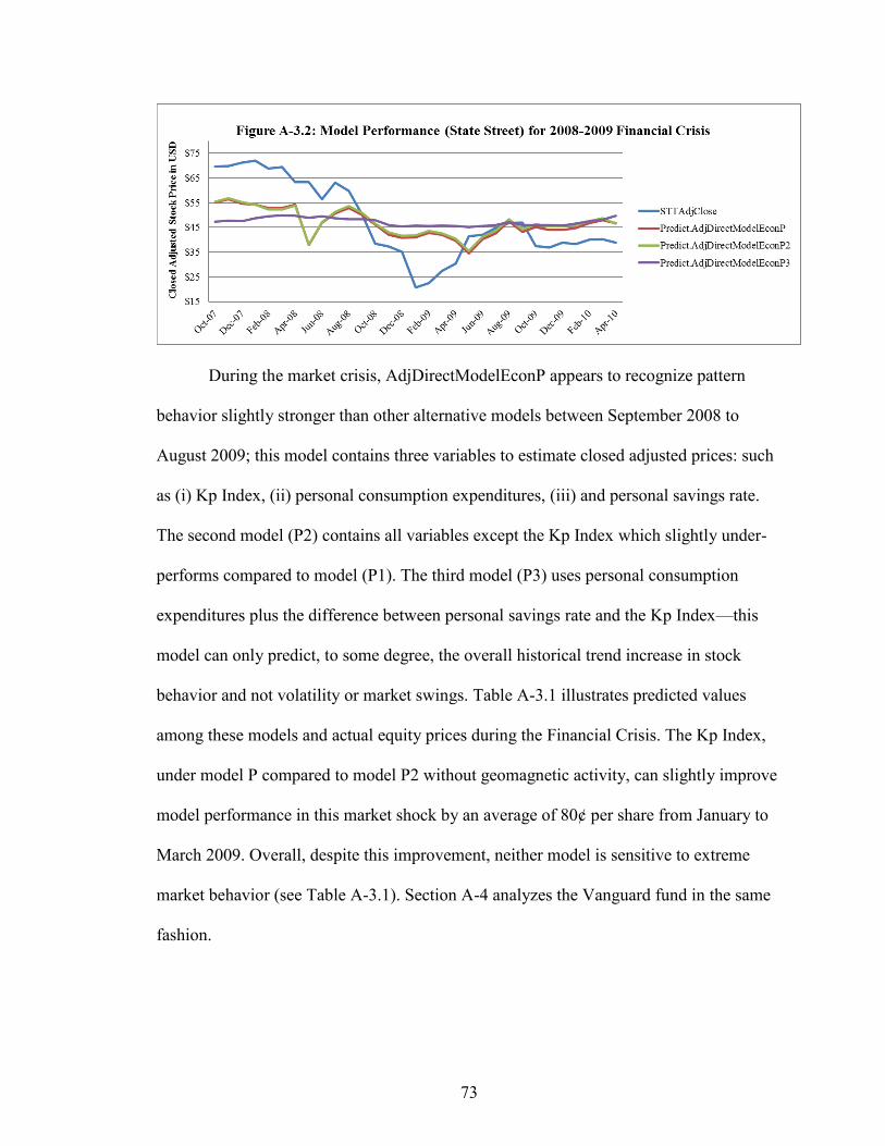
73
During the market crisis, AdjDirectModelEconP appears to recognize pattern
behavior slightly stronger than other alternative models between September 2008 to
August 2009; this model contains three variables to estimate closed adjusted prices: such
as (i) Kp Index, (ii) personal consumption expenditures, (iii) and personal savings rate.
The second model (P2) contains all variables except the Kp Index which slightly under-
performs compared to model (P1). The third model (P3) uses personal consumption
expenditures plus the difference between personal savings rate and the Kp Index—this
model can only predict, to some degree, the overall historical trend increase in stock
behavior and not volatility or market swings. Table A-3.1 illustrates predicted values
among these models and actual equity prices during the Financial Crisis. The Kp Index,
under model P compared to model P2 without geomagnetic activity, can slightly improve
model performance in this market shock by an average of 80¢ per share from January to
March 2009. Overall, despite this improvement, neither model is sensitive to extreme
market behavior (see Table A-3.1). Section A-4 analyzes the Vanguard fund in the same
fashion.

74
Table A-3.1: 2008-2009 Financial Crisis (STT) Predicted vs. Observed Prices
Column1 Dec-08 Jan-09 Feb-09 Mar-09 Apr-09 May-09
STTAdjClose (USD) 35.048183 20.736618 22.518881 27.437977 30.42424 41.406563
Predict.AdjDirectModelEconP (USD) 40.730626 41.048973 42.711146 42.0710226 39.739094 34.5756186
Predict.AdjDirectModelEconP2 (USD) 41.597521 41.866624 43.598454 42.684597 40.490221 35.4831193
Predict.AdjDirectModelEconP3 (USD) 45.29521 45.71013 45.51953 45.77006 45.45998 45.16978

75
Section A-4: Vanguard S&P 500 Robustness Analysis & Model Fitness
The Vanguard alternative models are using closed adjusted price data from October 1986 to November 2014 with the
exception of AdjDirectModelEconEMAP, which used 60 monthly periods after the 2008-2009 Financial Crisis at 2.7% MAPE.
The best historical performer, by MAPE, is AdjDirectModelEconP3 with an MAPE of 21.22%; Mod 2 & 3 have a MAPE of at
least 124%. As visualized, extreme swings in fund behavior (i.e., Van500IndexAdjClose) are not predicted accurately among
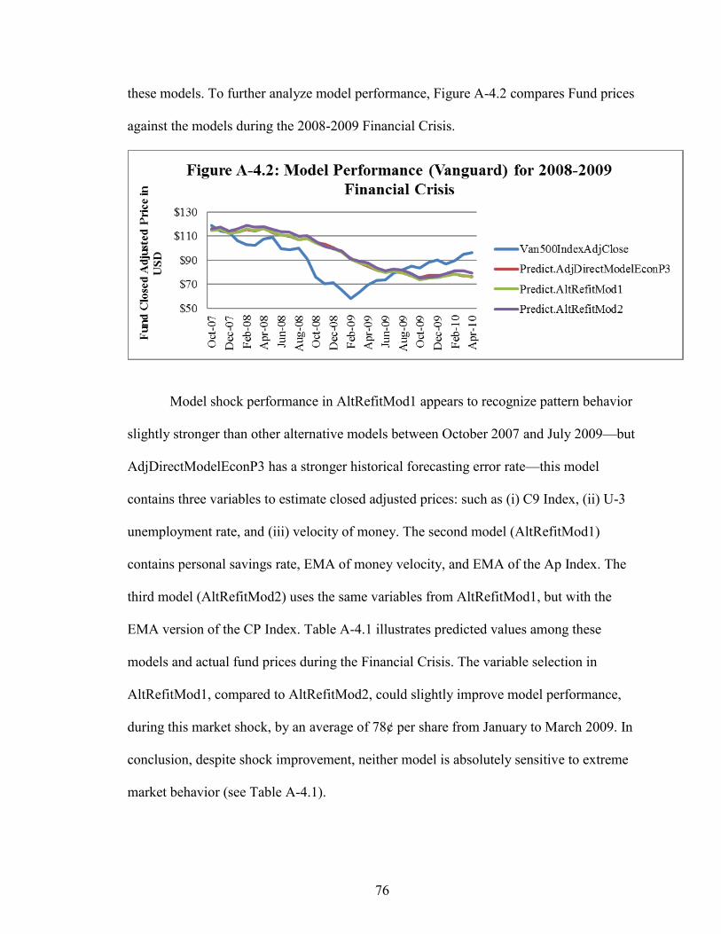
76
these models. To further analyze model performance, Figure A-4.2 compares Fund prices
against the models during the 2008-2009 Financial Crisis.
Model shock performance in AltRefitMod1 appears to recognize pattern behavior
slightly stronger than other alternative models between October 2007 and July 2009—but
AdjDirectModelEconP3 has a stronger historical forecasting error rate—this model
contains three variables to estimate closed adjusted prices: such as (i) C9 Index, (ii) U-3
unemployment rate, and (iii) velocity of money. The second model (AltRefitMod1)
contains personal savings rate, EMA of money velocity, and EMA of the Ap Index. The
third model (AltRefitMod2) uses the same variables from AltRefitMod1, but with the
EMA version of the CP Index. Table A-4.1 illustrates predicted values among these
models and actual fund prices during the Financial Crisis. The variable selection in
AltRefitMod1, compared to AltRefitMod2, could slightly improve model performance,
during this market shock, by an average of 78¢ per share from January to March 2009. In
conclusion, despite shock improvement, neither model is absolutely sensitive to extreme
market behavior (see Table A-4.1).
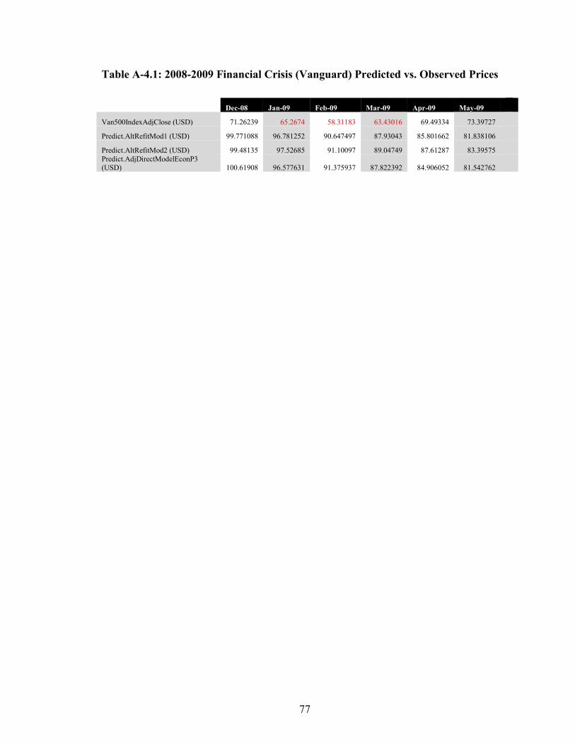
77
Table A-4.1: 2008-2009 Financial Crisis (Vanguard) Predicted vs. Observed Prices
Dec-08 Jan-09 Feb-09 Mar-09 Apr-09 May-09
Van500IndexAdjClose (USD) 71.26239 65.2674 58.31183 63.43016 69.49334 73.39727
Predict.AltRefitMod1 (USD) 99.771088 96.781252 90.647497 87.93043 85.801662 81.838106
Predict.AltRefitMod2 (USD) 99.48135 97.52685 91.10097 89.04749 87.61287 83.39575
Predict.AdjDirectModelEconP3
(USD) 100.61908 96.577631 91.375937 87.822392 84.906052 81.542762
78
Appendix B
Data Transformation Approach for Returns
This section will use transformed independent variables, outside absolute delta, in
time-series regression; the only exception in this exercise is that Fama-French’s market
parameters are not modified nor included in other models—this is to better understand
the variables’ impact before being included into the Fama-French Model for both State
Street stock and Vanguard S&P 500 Fund returns. Since most geomagnetic variables
have not shown promising results, they have undergone heavier data transformations
compared to the human economic behavioral variables. The objective of this analysis is
to understand if there is any meaningful information that can be used to improve the
Fama-French model. The data transformation methods are located in Chapter V. In
addition, the monthly time-series range is from October 1986 to November 2014. This
section will not follow typical equation patterns located in Chapter IV. Instead, the
analysis uses a linear regression matrix format, then compares the multiple outputs to the
Fama-French model. For variable elimination, the focus of the regression output includes
the following: (i) Adj. R2, (ii) RMSE (root-mean-squared-error), and (iii) p-values (0.1%,
1%, or 5%). A variance inflation factor (VIF) analysis will typically occur after the
model’s parameters have been adjusted (or removed). The following matrix is expressed
below:
Yt = Xt + t (15)

79
Section B-1: State Street Corporation Stock Returns
Table B-1.1: STT Transformed Data Approach, Part 1
TransModel 1 TransModel 2 TransModel 3 FFModel
========================================================
(Intercept) 9.79023 6.11946 -1.3108 -0.06705
(13.78657) (29.68894) (3.57921) (0.13014)
Kppwhalf 0.46999
(0.82055)
Appw8 0.00565
(0.02967)
Cppwnine -16.69977
(25.18379)
C9pwsqurt -0.03646
(0.11436)
KPLN 0.61833
(4.74959)
ApLn -0.34917
(1.40881)
CpLn 5.84214
(6.98404)
C9Ln -5.29675
(4.05846)
KpSqrt 0.05211
(0.94232)
APSqrt -0.19308
(0.75467)
CpSqrt 24.04645
(26.37132)
C9Squrt -10.42755
(8.34498)
MktRF 0.36832 ***
(0.02967)
SMB -0.09350 *
(0.04236)
HML 0.21147 ***
(0.04613)
------------------------------------------------------------------------------------------------
R^2 0.00182 0.00844 0.00576 0.32647
Adj. R^2 -0.01017 -0.00347 -0.00619 0.32042
Num. obs. 338 338 338 338
RMSE 2.86964 2.8601 2.86397 2.3537
========================================================
*** p < 0.001, ** p < 0.01, * p < 0.05
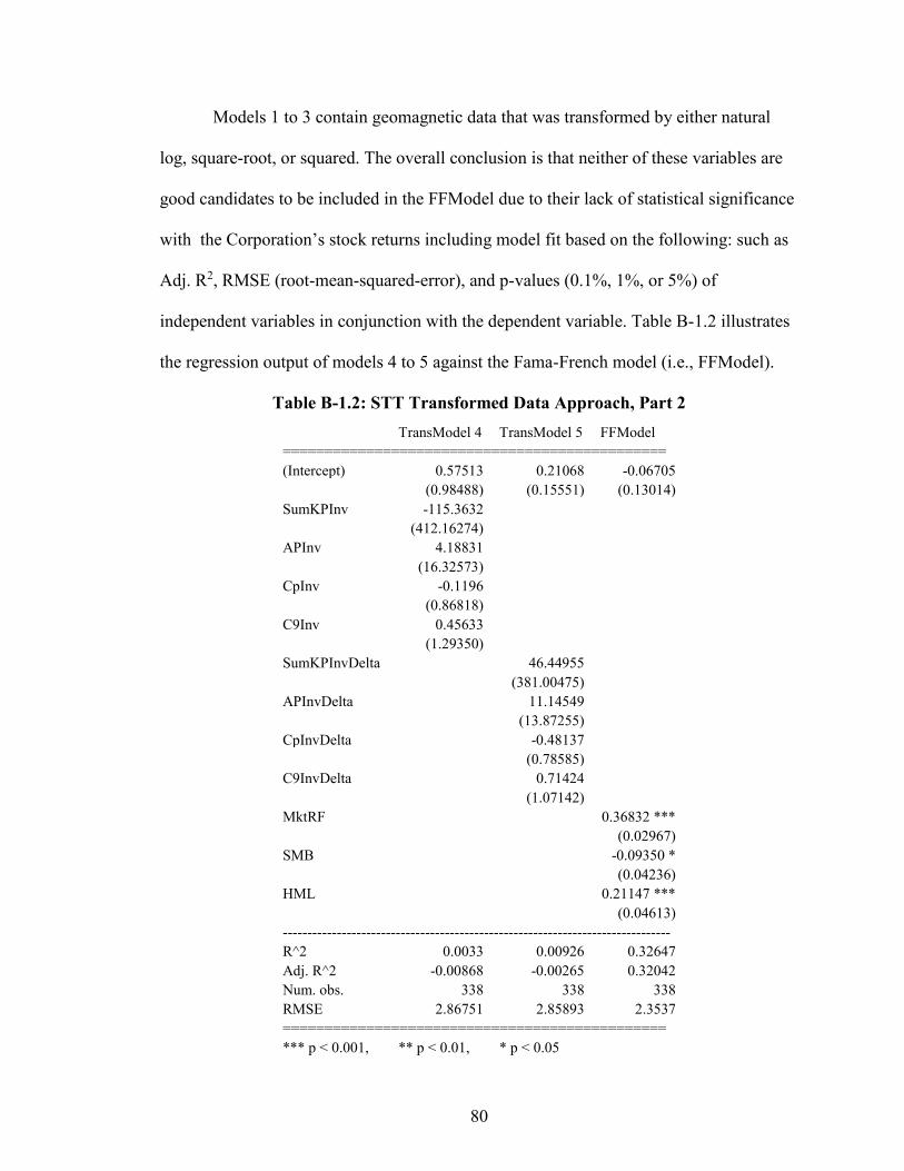
80
Models 1 to 3 contain geomagnetic data that was transformed by either natural
log, square-root, or squared. The overall conclusion is that neither of these variables are
good candidates to be included in the FFModel due to their lack of statistical significance
with the Corporation’s stock returns including model fit based on the following: such as
Adj. R2, RMSE (root-mean-squared-error), and p-values (0.1%, 1%, or 5%) of
independent variables in conjunction with the dependent variable. Table B-1.2 illustrates
the regression output of models 4 to 5 against the Fama-French model (i.e., FFModel).
Table B-1.2: STT Transformed Data Approach, Part 2
TransModel 4 TransModel 5 FFModel
==============================================
(Intercept) 0.57513 0.21068 -0.06705
(0.98488) (0.15551) (0.13014)
SumKPInv -115.3632
(412.16274)
APInv 4.18831
(16.32573)
CpInv -0.1196
(0.86818)
C9Inv 0.45633
(1.29350)
SumKPInvDelta 46.44955
(381.00475)
APInvDelta 11.14549
(13.87255)
CpInvDelta -0.48137
(0.78585)
C9InvDelta 0.71424
(1.07142)
MktRF 0.36832 ***
(0.02967)
SMB -0.09350 *
(0.04236)
HML 0.21147 ***
(0.04613)
-------------------------------------------------------------------------------
R^2 0.0033 0.00926 0.32647
Adj. R^2 -0.00868 -0.00265 0.32042
Num. obs. 338 338 338
RMSE 2.86751 2.85893 2.3537
==============================================
*** p < 0.001, ** p < 0.01, * p < 0.05

81
As defined in Chapter V, TransModel 4 takes on the rate for geomagnetic activity
at (1 ÷ xt). TransModel 5 uses the derivative calculated in TransModel 4 where each
variable is then transformed into its delta form. Overall, neither of these variables have
revealed any parameter significance with single stock returns including overall model fit;
therefore, neither of the transformed variables are included in the Fama-French model for
model performance analysis. The next section will follow the same approach with these
transformed parameters, but within a larger market environment.
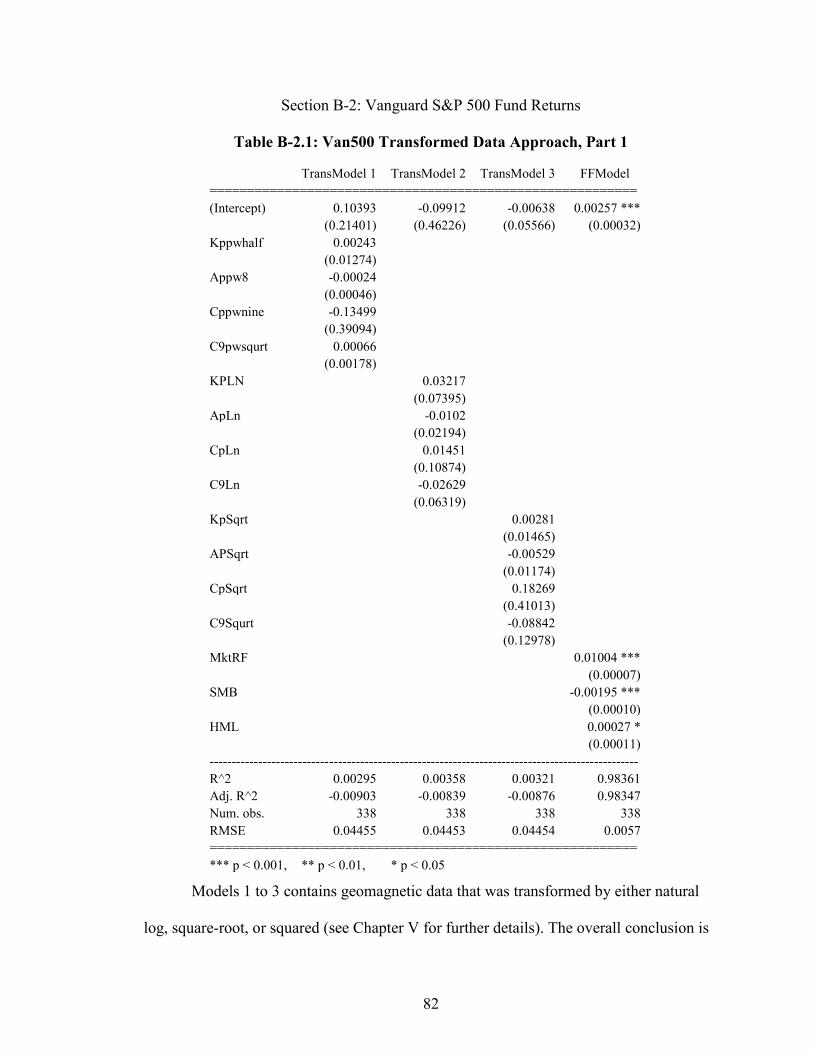
82
Section B-2: Vanguard S&P 500 Fund Returns
Table B-2.1: Van500 Transformed Data Approach, Part 1
Models 1 to 3 contains geomagnetic data that was transformed by either natural
log, square-root, or squared (see Chapter V for further details). The overall conclusion is
TransModel 1 TransModel 2 TransModel 3 FFModel
=========================================================
(Intercept) 0.10393 -0.09912 -0.00638 0.00257 ***
(0.21401) (0.46226) (0.05566) (0.00032)
Kppwhalf 0.00243
(0.01274)
Appw8 -0.00024
(0.00046)
Cppwnine -0.13499
(0.39094)
C9pwsqurt 0.00066
(0.00178)
KPLN 0.03217
(0.07395)
ApLn -0.0102
(0.02194)
CpLn 0.01451
(0.10874)
C9Ln -0.02629
(0.06319)
KpSqrt 0.00281
(0.01465)
APSqrt -0.00529
(0.01174)
CpSqrt 0.18269
(0.41013)
C9Squrt -0.08842
(0.12978)
MktRF 0.01004 ***
(0.00007)
SMB -0.00195 ***
(0.00010)
HML 0.00027 *
(0.00011)
-------------------------------------------------------------------------------------------------
R^2 0.00295 0.00358 0.00321 0.98361
Adj. R^2 -0.00903 -0.00839 -0.00876 0.98347
Num. obs. 338 338 338 338
RMSE 0.04455 0.04453 0.04454 0.0057
=========================================================
*** p < 0.001, ** p < 0.01, * p < 0.05
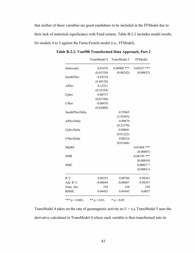
83
that neither of these variables are good candidates to be included in the FFModel due to
their lack of statistical significance with Fund returns. Table B-2.2 includes model results
for models 4 to 5 against the Fama-French model (i.e., FFModel).
Table B-2.2: Van500 Transformed Data Approach, Part 2
TransModel 4 TransModel 5 FFModel
===============================================
(Intercept) 0.01676 0.00900 *** 0.00257 ***
(0.01530) (0.00242) (0.00032)
SumKPInv -4.85218
(6.40120)
APInv 0.12521
(0.25354)
CpInv 0.00737
(0.01348)
C9Inv -0.00976
(0.02009)
SumKPInvDelta -0.55865
(5.92493)
APInvDelta 0.09679
(0.21570)
CpInvDelta -0.00041
(0.01222)
C9InvDelta 0.00216
(0.01666)
MktRF 0.01004 ***
(0.00007)
SMB -0.00195 ***
(0.00010)
HML 0.00027 *
(0.00011)
-------------------------------------------------------------------------------
R^2 0.00353 0.00706 0.98361
Adj. R^2 -0.00844 -0.00487 0.98347
Num. obs. 338 338 338
RMSE 0.04453 0.04445 0.0057
===============================================
*** p < 0.001, ** p < 0.01, * p < 0.05
TransModel 4 takes on the rate of geomagnetic activity at (1 ÷ xt). TransModel 5 uses the
derivative calculated in TransModel 4 where each variable is then transformed into its

84
delta form. Overall, neither variable tested provides any statistical significance to be
included into the Fama-French model for model performance analysis.
Overall, the data transformation approach for both dependent variables revealed
that neither parameter could improve model estimation due to insignificant p-values with
its dependent variable. The next appendix discusses the Granger test for causality.

85
Appendix C
Causality of Earth’s Magnetic Field and Human Economic Behavior
To test causality among the geomagnetic field indices and the proposed human
economic behavioral variables, the Granger Causality test is utilized. The human
economic variables includes their raw monthly average form. Each variable is tested
separately and not through multivariate analyses which uses vector auto-regression. The
final result does not necessarily warrant a 100% certainty that X causes Y—but,
according to Granger (1988), the method may reveal a causal relationship of causality
between or among variables for prediction—this research is statistically trying to show if
there is enough information in X that could help predict Y. In addition, optimal lag order,
for each variable, is revealed through this test. A p-value near (or above) 5% suggests no
causality between the variables (i.e., fail to reject the null hypothesis). The test will also
use a reverse approach were the independent variable becomes dependent, as well as the
dependent to independent.
After all variables were tested, the analysis indicated that geomagnetic activity
does not Granger-cause human economic behavior—this is also true for the reverse
approach. Despite the results not adhering to minimal standards, the Cp and Ap indices
were closest to testing positive for causality with personal savings rate at 9.3% and 6.2%,
respectively. Table C-1 illustrates the results for this test. The time-series is from October
1986 to November 2014 for all raw monthly averaged data.

86
Table C-1: Results for Causality of Earth’s Magnetic Field and Human Economic Behavior2
Independent
Variable Dependent Variable
P-
Value Reject Null?
Lag
Order
Reverse
Order P-
Val
Reverse
Order
Lag
Reject Null?
SumKp Money Velocity 0.6364 Fail to Reject 1 0.2988 9 Fail to Reject
CP Money Velocity 0.5788 Fail to Reject 1 0.1843 12 Fail to Reject
AP Money Velocity 0.6618 Fail to Reject 1 0.6029 7 Fail to Reject
C9 Money Velocity 0.6431 Fail to Reject 1 0.1299 12 Fail to Reject
SumKp U-3 Unemployment 0.2886 Fail to Reject 11 0.3998 1 Fail to Reject
CP U-3 Unemployment 0.1896 Fail to Reject 11 0.4171 1 Fail to Reject
AP U-3 Unemployment 0.7216 Fail to Reject 11 0.615 1 Fail to Reject
C9 U-3 Unemployment 0.267 Fail to Reject 17 0.4169 1 Fail to Reject
SumKp Personal Savings Rate 0.1179 Fail to Reject 19 0.2137 1 Fail to Reject
CP Personal Savings Rate 0.0929 Fail to Reject 19 0.1547 1 Fail to Reject
AP Personal Savings Rate 0.06207 Fail to Reject 19 0.5498 1 Fail to Reject
C9 Personal Savings Rate 0.1639 Fail to Reject 19 0.141 1 Fail to Reject
SumKp Personal Consumption 0.331 Fail to Reject 22 0.2359 1 Fail to Reject
CP Personal Consumption 0.3154 Fail to Reject 21 0.2497 1 Fail to Reject
AP Personal Consumption 0.7591 Fail to Reject 1 0.3714 1 Fail to Reject
C9 Personal Consumption 0.3164 Fail to Reject 21 0.2278 1 Fail to Reject
2 (Zeileis & Hothorn 2002)
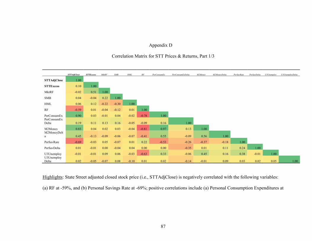
87
Appendix D
Correlation Matrix for STT Prices & Returns, Part 1/3
STTAdjClose STTExcess MktRF SMB HML RF PerConsumEx PerConsumExDelta M2Money M2MoneyDelta PerSavRate PerSavDelta U3Unemploy U3UnemployDelta
STTAdjClose 1.00
STTExcess 0.10 1.00
MktRF -0.02 0.51 1.00
SMB 0.04 -0.04 0.22 1.00
HML 0.06 0.12 -0.22 -0.30 1.00
RF -0.59 0.01 -0.04 -0.12 0.01 1.00
PerConsumEx 0.90 0.03 -0.01 0.04 -0.02 -0.78 1.00
PerConsumEx
Delta 0.19 0.11 0.13 0.16 -0.05 -0.09 0.16 1.00
M2Money 0.83 0.04 0.02 0.03 -0.04 -0.81 0.97 0.13 1.00 M2MoneyDelt
a 0.45 -0.13 -0.09 -0.06 -0.07 -0.41 0.55 -0.09 0.56 1.00
PerSavRate -0.69 -0.03 0.05 -0.07 0.01 0.22 -0.53 -0.26 -0.37 -0.18 1.00
PerSavDelta 0.01 -0.01 0.00 -0.04 0.04 0.00 0.00 -0.35 0.01 0.11 0.24 1.00
U3Unemploy -0.01 -0.01 0.09 0.06 -0.03 -0.63 0.33 -0.06 0.45 0.16 0.38 -0.01 1.00
U3UnemployDelta 0.02 -0.05 -0.07 0.08 -0.10 0.01 0.02 -0.14 -0.01 0.09 0.03 0.02 0.05 1.00
Highlights: State Street adjusted closed stock price (i.e., STTAdjClose) is negatively correlated with the following variables:
(a) RF at -59%, and (b) Personal Savings Rate at -69%; positive correlations include (a) Personal Consumption Expenditures at

88
90%, (b) Velocity of Money at 83%, and (c) the absolute change in the Velocity of
Money at 45%. For State Street stock returns (i.e., STTExcess), the Fama-French factor
MktRF tested positive at 51%.

89
Correlation Matrix for STT Prices & Returns, Part 2/3
STTAdjClose STTExcess SumKp Kppwhalf KPLN SumKPDelta SumKPInv SumKPInvDelta Ap Appw8 ApLn APSqrt APDelta APInv APInvDelta
STTAdjClose 1.00
STTExcess 0.10 1.00
SumKp -0.47 0.00 1.00
Kppwhalf -0.47 0.00 0.99 1.00
KPLN -0.46 0.00 0.97 0.99 1.00
SumKPDelta -0.01 -0.08 0.32 0.30 0.28 1.00
SumKPInv 0.40 0.00 -0.87 -0.91 -0.96 -0.22 1.00
SumKPInvDelta 0.00 0.08 -0.24 -0.25 -0.27 -0.75 0.30 1.00
Ap -0.39 0.01 0.94 0.91 0.87 0.39 -0.73 -0.24 1.00
Appw8 -0.37 0.01 0.92 0.88 0.83 0.40 -0.69 -0.23 1.00 1.00
ApLn -0.43 0.00 0.97 0.98 0.97 0.34 -0.90 -0.28 0.94 0.91 1.00
APSqrt -0.42 0.01 0.97 0.96 0.93 0.37 -0.82 -0.26 0.99 0.97 0.98 1.00
APDelta -0.01 -0.08 0.27 0.25 0.22 0.89 -0.16 -0.55 0.43 0.45 0.32 0.38 1.00
APInv 0.38 0.00 -0.87 -0.92 -0.95 -0.25 0.99 0.30 -0.77 -0.73 -0.93 -0.86 -0.21 1.00
APInvDelta 0.01 0.09 -0.25 -0.26 -0.27 -0.77 0.29 0.95 -0.28 -0.27 -0.32 -0.30 -0.65 0.33 1.00
Highlights: State Street adjusted closed stock price (i.e., STTAdjClose) is negatively correlated with the following
geomagnetic variables: (a) SumKp at -47%, (b) Kppwhalf at -47%, (c) KPLN at -46%, (d) Ap at -39%, (e) Appw8 at -37%, (f)
ApLn at -43%, and (g) ApSqrt at -42%; positive correlations include (a) SumKPInv at 40% and (b) APInv at 38%. For State
Street stock returns (i.e., STTExcess), nothing significant was revealed.
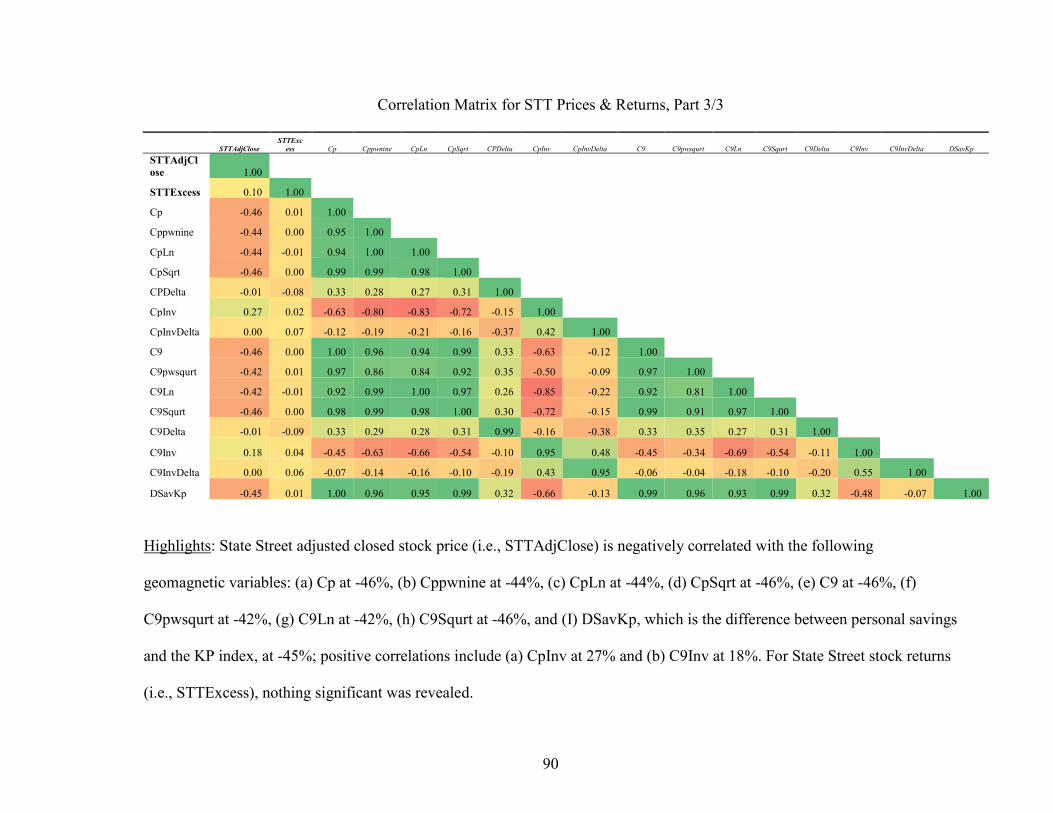
90
Correlation Matrix for STT Prices & Returns, Part 3/3
STTAdjClose
STTExc
ess Cp Cppwnine CpLn CpSqrt CPDelta CpInv CpInvDelta C9 C9pwsqurt C9Ln C9Squrt C9Delta C9Inv C9InvDelta DSavKp
STTAdjCl
ose 1.00
STTExcess 0.10 1.00
Cp -0.46 0.01 1.00
Cppwnine -0.44 0.00 0.95 1.00
CpLn -0.44 -0.01 0.94 1.00 1.00
CpSqrt -0.46 0.00 0.99 0.99 0.98 1.00
CPDelta -0.01 -0.08 0.33 0.28 0.27 0.31 1.00
CpInv 0.27 0.02 -0.63 -0.80 -0.83 -0.72 -0.15 1.00
CpInvDelta 0.00 0.07 -0.12 -0.19 -0.21 -0.16 -0.37 0.42 1.00
C9 -0.46 0.00 1.00 0.96 0.94 0.99 0.33 -0.63 -0.12 1.00
C9pwsqurt -0.42 0.01 0.97 0.86 0.84 0.92 0.35 -0.50 -0.09 0.97 1.00
C9Ln -0.42 -0.01 0.92 0.99 1.00 0.97 0.26 -0.85 -0.22 0.92 0.81 1.00
C9Squrt -0.46 0.00 0.98 0.99 0.98 1.00 0.30 -0.72 -0.15 0.99 0.91 0.97 1.00
C9Delta -0.01 -0.09 0.33 0.29 0.28 0.31 0.99 -0.16 -0.38 0.33 0.35 0.27 0.31 1.00
C9Inv 0.18 0.04 -0.45 -0.63 -0.66 -0.54 -0.10 0.95 0.48 -0.45 -0.34 -0.69 -0.54 -0.11 1.00
C9InvDelta 0.00 0.06 -0.07 -0.14 -0.16 -0.10 -0.19 0.43 0.95 -0.06 -0.04 -0.18 -0.10 -0.20 0.55 1.00
DSavKp -0.45 0.01 1.00 0.96 0.95 0.99 0.32 -0.66 -0.13 0.99 0.96 0.93 0.99 0.32 -0.48 -0.07 1.00
Highlights: State Street adjusted closed stock price (i.e., STTAdjClose) is negatively correlated with the following
geomagnetic variables: (a) Cp at -46%, (b) Cppwnine at -44%, (c) CpLn at -44%, (d) CpSqrt at -46%, (e) C9 at -46%, (f)
C9pwsqurt at -42%, (g) C9Ln at -42%, (h) C9Squrt at -46%, and (I) DSavKp, which is the difference between personal savings
and the KP index, at -45%; positive correlations include (a) CpInv at 27% and (b) C9Inv at 18%. For State Street stock returns
(i.e., STTExcess), nothing significant was revealed.
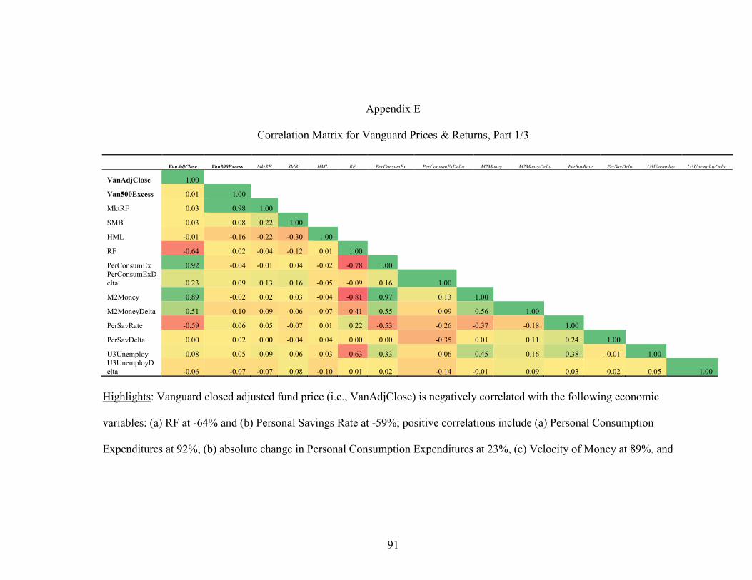
91
Appendix E
Correlation Matrix for Vanguard Prices & Returns, Part 1/3
VanAdjClose Van500Excess MktRF SMB HML RF PerConsumEx PerConsumExDelta M2Money M2MoneyDelta PerSavRate PerSavDelta U3Unemploy U3UnemployDelta
VanAdjClose 1.00
Van500Excess 0.01 1.00
MktRF 0.03 0.98 1.00
SMB 0.03 0.08 0.22 1.00
HML -0.01 -0.16 -0.22 -0.30 1.00
RF -0.64 0.02 -0.04 -0.12 0.01 1.00
PerConsumEx 0.92 -0.04 -0.01 0.04 -0.02 -0.78 1.00
PerConsumExD
elta 0.23 0.09 0.13 0.16 -0.05 -0.09 0.16 1.00
M2Money 0.89 -0.02 0.02 0.03 -0.04 -0.81 0.97 0.13 1.00
M2MoneyDelta 0.51 -0.10 -0.09 -0.06 -0.07 -0.41 0.55 -0.09 0.56 1.00
PerSavRate -0.59 0.06 0.05 -0.07 0.01 0.22 -0.53 -0.26 -0.37 -0.18 1.00
PerSavDelta 0.00 0.02 0.00 -0.04 0.04 0.00 0.00 -0.35 0.01 0.11 0.24 1.00
U3Unemploy 0.08 0.05 0.09 0.06 -0.03 -0.63 0.33 -0.06 0.45 0.16 0.38 -0.01 1.00 U3UnemployD
elta -0.06 -0.07 -0.07 0.08 -0.10 0.01 0.02 -0.14 -0.01 0.09 0.03 0.02 0.05 1.00
Highlights: Vanguard closed adjusted fund price (i.e., VanAdjClose) is negatively correlated with the following economic
variables: (a) RF at -64% and (b) Personal Savings Rate at -59%; positive correlations include (a) Personal Consumption
Expenditures at 92%, (b) absolute change in Personal Consumption Expenditures at 23%, (c) Velocity of Money at 89%, and

92
(d) the absolute change in the Velocity of Money at 51%. For Vanguard fund returns (i.e.,
Van500Excess), the Fama-French factor MktRF tested positive at 98%.
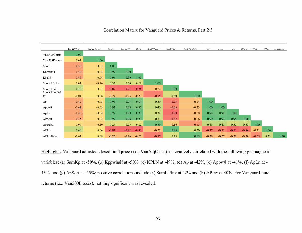
93
Correlation Matrix for Vanguard Prices & Returns, Part 2/3
VanAdjClose Van500Excess SumKp Kppwhalf KPLN SumKPDelta SumKPInv SumKPInvDelta Ap Appw8 ApLn APSqrt APDelta APInv APInvDelta
VanAdjClose 1.00
Van500Excess 0.01 1.00
SumKp -0.50 -0.03 1.00
Kppwhalf -0.50 -0.04 0.99 1.00
KPLN -0.49 -0.04 0.97 0.99 1.00
SumKPDelta 0.01 -0.10 0.32 0.30 0.28 1.00
SumKPInv 0.42 0.04 -0.87 -0.91 -0.96 -0.22 1.00 SumKPInvDel
ta -0.01 0.08 -0.24 -0.25 -0.27 -0.75 0.30 1.00
Ap -0.42 -0.03 0.94 0.91 0.87 0.39 -0.73 -0.24 1.00
Appw8 -0.41 -0.03 0.92 0.88 0.83 0.40 -0.69 -0.23 1.00 1.00
ApLn -0.45 -0.04 0.97 0.98 0.97 0.34 -0.90 -0.28 0.94 0.91 1.00
APSqrt -0.45 -0.04 0.97 0.96 0.93 0.37 -0.82 -0.26 0.99 0.97 0.98 1.00
APDelta 0.00 -0.10 0.27 0.25 0.22 0.89 -0.16 -0.55 0.43 0.45 0.32 0.38 1.00
APInv 0.40 0.04 -0.87 -0.92 -0.95 -0.25 0.99 0.30 -0.77 -0.73 -0.93 -0.86 -0.21 1.00
APInvDelta -0.01 0.08 -0.25 -0.26 -0.27 -0.77 0.29 0.95 -0.28 -0.27 -0.32 -0.30 -0.65 0.33 1.00
Highlights: Vanguard adjusted closed fund price (i.e., VanAdjClose) is negatively correlated with the following geomagnetic
variables: (a) SumKp at -50%, (b) Kppwhalf at -50%, (c) KPLN at -49%, (d) Ap at -42%, (e) Appw8 at -41%, (f) ApLn at -
45%, and (g) ApSqrt at -45%; positive correlations include (a) SumKPInv at 42% and (b) APInv at 40%. For Vanguard fund
returns (i.e., Van500Excess), nothing significant was revealed.

94
Correlation Matrix for Vanguard Prices & Returns, Part 3/3
VanAdjClose Van500Excess Cp Cppwnine CpLn CpSqrt CPDelta CpInv CpInvDelta C9 C9pwsqurt C9Ln C9Squrt C9Delta C9Inv C9InvDelta
VanAdjClose 1.00
Van500Excess 0.01 1.00
Cp -0.49 -0.03 1.00
Cppwnine -0.47 -0.04 0.95 1.00
CpLn -0.46 -0.04 0.94 1.00 1.00
CpSqrt -0.49 -0.04 0.99 0.99 0.98 1.00
CPDelta 0.00 -0.09 0.33 0.28 0.27 0.31 1.00
CpInv 0.28 0.04 -0.63 -0.80 -0.83 -0.72 -0.15 1.00
CpInvDelta 0.00 0.08 -0.12 -0.19 -0.21 -0.16 -0.37 0.42 1.00
C9 -0.49 -0.03 1.00 0.96 0.94 0.99 0.33 -0.63 -0.12 1.00
C9pwsqurt -0.46 -0.02 0.97 0.86 0.84 0.92 0.35 -0.50 -0.09 0.97 1.00
C9Ln -0.45 -0.04 0.92 0.99 1.00 0.97 0.26 -0.85 -0.22 0.92 0.81 1.00
C9Squrt -0.49 -0.04 0.98 0.99 0.98 1.00 0.30 -0.72 -0.15 0.99 0.91 0.97 1.00
C9Delta 0.00 -0.10 0.33 0.29 0.28 0.31 0.99 -0.16 -0.38 0.33 0.35 0.27 0.31 1.00
C9Inv 0.19 0.03 -0.45 -0.63 -0.66 -0.54 -0.10 0.95 0.48 -0.45 -0.34 -0.69 -0.54 -0.11 1.00
C9InvDelta 0.00 0.06 -0.07 -0.14 -0.16 -0.10 -0.19 0.43 0.95 -0.06 -0.04 -0.18 -0.10 -0.20 0.55 1.00
Highlights: Vanguard adjusted closed fund price (i.e., VanAdjClose) is negatively correlated with the following geomagnetic
variables: (a) Cp at -49%, (b) Cppwnine at -47%, (c) CpLn at -46%, (d) CpSqrt at -49%, (e) C9 at -49%, (f) C9pwsqurt at -
46%, (g) C9Ln at -45%, and (h) C9Squrt at -49%; positive correlations include (a) CpInv at 28% and (b) C9Inv at 19%. For
Vanguard fund returns (i.e., Van500Excess), nothing significant was revealed.
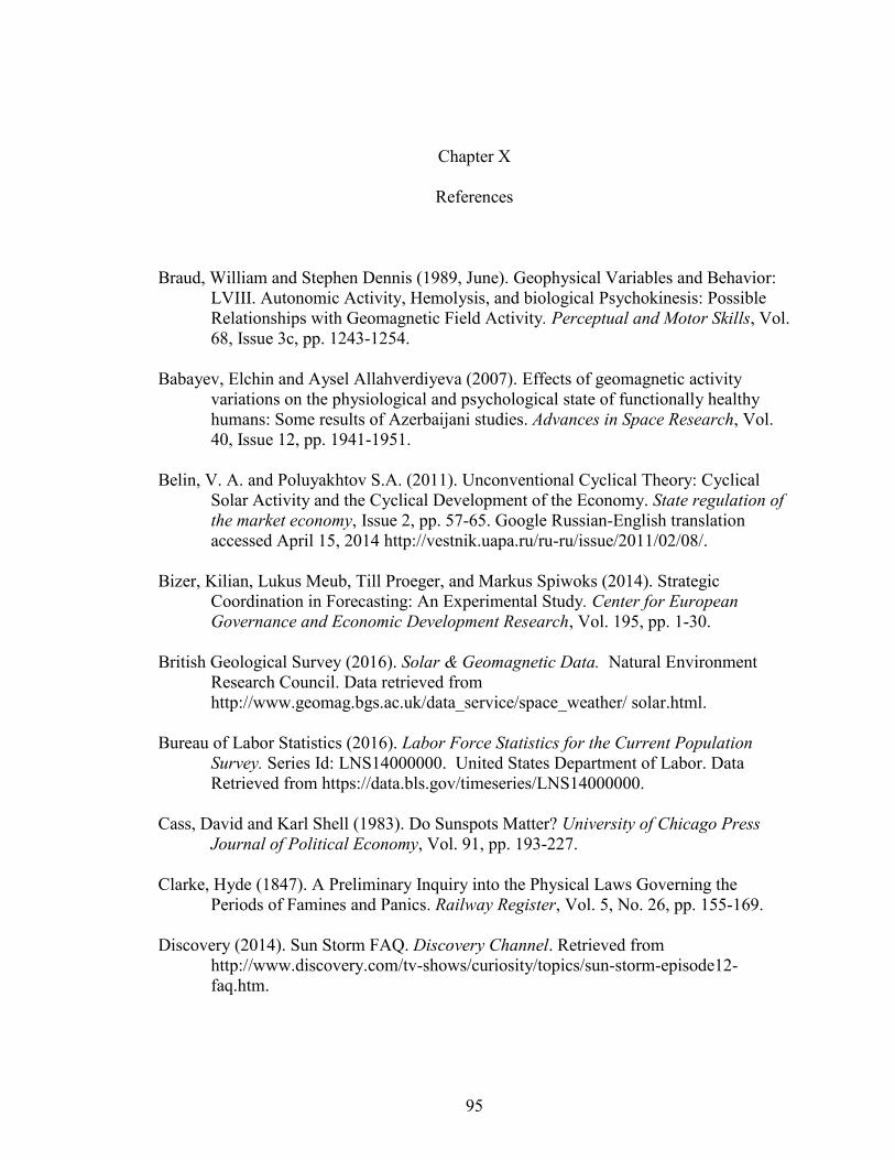
95
Chapter X
References
Braud, William and Stephen Dennis (1989, June). Geophysical Variables and Behavior:
LVIII. Autonomic Activity, Hemolysis, and biological Psychokinesis: Possible
Relationships with Geomagnetic Field Activity. Perceptual and Motor Skills, Vol.
68, Issue 3c, pp. 1243-1254.
Babayev, Elchin and Aysel Allahverdiyeva (2007). Effects of geomagnetic activity
variations on the physiological and psychological state of functionally healthy
humans: Some results of Azerbaijani studies. Advances in Space Research, Vol.
40, Issue 12, pp. 1941-1951.
Belin, V. A. and Poluyakhtov S.A. (2011). Unconventional Cyclical Theory: Cyclical
Solar Activity and the Cyclical Development of the Economy. State regulation of
the market economy, Issue 2, pp. 57-65. Google Russian-English translation
accessed April 15, 2014 http://vestnik.uapa.ru/ru-ru/issue/2011/02/08/.
Bizer, Kilian, Lukus Meub, Till Proeger, and Markus Spiwoks (2014). Strategic
Coordination in Forecasting: An Experimental Study. Center for European
Governance and Economic Development Research, Vol. 195, pp. 1-30.
British Geological Survey (2016). Solar & Geomagnetic Data. Natural Environment
Research Council. Data retrieved from
http://www.geomag.bgs.ac.uk/data_service/space_weather/ solar.html.
Bureau of Labor Statistics (2016). Labor Force Statistics for the Current Population
Survey. Series Id: LNS14000000. United States Department of Labor. Data
Retrieved from https://data.bls.gov/timeseries/LNS14000000.
Cass, David and Karl Shell (1983). Do Sunspots Matter? University of Chicago Press
Journal of Political Economy, Vol. 91, pp. 193-227.
Clarke, Hyde (1847). A Preliminary Inquiry into the Physical Laws Governing the
Periods of Famines and Panics. Railway Register, Vol. 5, No. 26, pp. 155-169.
Discovery (2014). Sun Storm FAQ. Discovery Channel. Retrieved from
http://www.discovery.com/tv-shows/curiosity/topics/sun-storm-episode12-
faq.htm.

96
Dougal-Roney, S.M. and Gunther Vogal (1990). Some Speculations of the effect of
Geomagnetism on the Pineal Gland. PSI Research Center. Retrieved from
http://www.psi-researchcentre.co.uk/article_10.htm.
East, Jackie R (2014). Natural Phenomena as Potential Influence on Social and Political
Behavior: The Earth’s Magnetic Field (Doctoral Dissertation). Retrieved from
http://uknowledge.uky.edu/polysci_etds/11. (Paper 11).
Fama, Eugene and Kenneth French (1992). The Cross-Section of Expected Stock
Returns. The Journal of Finance, Vol. 47, Issue 2, pp. 427-465.
Fama, Eugene and Kenneth French (1993). Common Risk Factors in the Returns on
Stocks and Bonds. Journal of Financial Economics, Vol. 33, pp. 3-56.
Fama, Eugene and Kenneth French (2015). A five-factor asset pricing model. Journal of
Financial Economics, Vol. 116, Issue 1, pp. 1-22.
Fama, Eugene (2016). Data Library. Dartmouth Tuck School of Business. Data retrieved
from http://mba.tuck.dartmouth.edu/pages/faculty/ken.french/data_library.html.
Federal Reserve Bank of St. Louis (2016). Personal Saving Rate, Percent, Monthly,
Seasonally Adjusted Annual Rate. Federal Reserve Economic Data. Data retrieved
from https://fred.stlouisfed.org.
Federal Reserve Bank of St. Louis (2016). Personal Consumption Expenditures, Billions
of Dollars, Monthly, Seasonally Adjusted Annual Rate. Economic Research
Division. Data retrieved from https://fred.stlouisfed.org.
Federal Reserve Bank of St. Louis (2016). M2 Money Stock, Billions of Dollars, Monthly,
Seasonally Adjusted. Economic Research Division. Data retrieved from
https://fred.stlouisfed.org.
Gorbanev, Mikhail (2012). Sunspots, Unemployment, and Recessions, or Can the Solar
Activity Cycle Shape the Business Cycle? Munich Personal RePEc Archive, No.
40271, pp. 1-36.
Gilbert, William (1958). De Magnete. (P. Fleury Mottelay, Trans.). New York, NY:
Dover. (Original work published in 1600).
Granger, C.W.J. (1988). Some recent development in a concept of causality. Journal of
Econometrics, Vol. 39, Issue 1-2 pp. 199-211.
Hans, J.L. (2003). The Large-Scale Magnetic Field Structure of our Galaxy: Efficiently
Deduced from Pulsar Rotation Measures. In: Uyaniker, B., Reich, W.,
Wielebinksi, R. The Magnetized Interstellar Medium. Antalya, Turkey. pp. 3-12.

97
Hutson, Jack (1984). Filter Price Data: Moving Averages vs. Exponential Moving
Averages. Stocks & Commodities, Vol. 2, Issue 3, pp. 102-103.
Hyndman, RJ (2017). forecast: Forecasting functions for time series and linear models.
R package version 8.0. Retrieved from https://cran.r-
project.org/web/packages/forecast/.
IMDb (2016). Star Wars: Episode IV – A New Hope (1977). Quotes.
http://www.imdb.com/title/tt0076759/quotes.
Ivory, Kevin (2016). Geomagnetic ap, AP, CP, and C9 Indices. The Max Planck Society.
Retrieved from http://wwwuser.gwdg.de/~rhennin/ap.html.
Jevons, W.S. (1878, Nov). Commercial Crises and Sun-Spots. Nature, Vol. 19, pp. 33-37.
Karasek M, Woldanska-Okonska M, Czernicki J, Zylinska K, Swietoslawski J (1998).
Chronic Exposure to 2.9 mT, 40Hz Magnetic Field Reduces Melatonin
Concentrations in Humans. Journal of Pineal Research, Vol. 25, Issue 4, 240-
244.
Krieg, Melanie (2008-2009). “Star Wars”: The Strategic Defense Initiative. UC David
Prized Writing. http://prizedwriting.ucdavis.edu/past/2008-2009/201cstar-
wars201d-the-strategic-defense-initiative.
LA Times (2011). ‘Star Wars’: A Look Back on Opening Day in May 1977. Hero
Complex. http://herocomplex.latimes.com/movies/star-wars-a-look-back-on-
opening-day-in-may-1977/.
Lanza, Roberto and Antonio Meloni (2006). The Earth’s Magnetism: An Introduction for
Geologists. New York, NY: Springer. pp. 1-267.
Leifeld, Philip (2013). texreg: Conversion of Statistical Model Output in R to LaTeX and
HTML Tables. R package version 2.15.0. https://cran.r-project.org/web/packages
/texreg/index.html.
Linter, John (1965a). Security Prices, Risk, and Maximal From Diversification. The
Journal of Finance, Vol. 20, Issue 4, pp. 587-615.
Linter, John (1965b). The Valuation of Risk Assets and the Selection of Risky
Investments in Stock Portfolios and Capital Budgets. The Review of Economics
and Statistics, Vol. 47, Issue 1, pp. 13-37.
Martin, T. (2008). Bully Pulpits and Financial Markets: Presidential Influence of Wall
Street (Doctoral Dissertation). University of Kentucky.

98
Modis, Theodore (2007, June). Sunspots, GDP and the Stock Market. Technological
Forecasting & Social Change, Vol. 74: pp. 1508-1514.
Mossin, Jan (1966). Equilibrium in a Capital Asset Market. The Econometric Society,
Vol. 34, Issue 4, pp. 768-783.
Myttenaere, Arnaud De, Boris Golden, Benedicte Le Grand, and Fabrice Rossi (2015,
June). Using the Mean Absolute Percentage Error for Regression Models. Cornell
University Library, pp.1-7 . Retrieved from https://arxiv.org/abs/1506.04176v1.
NOAA (2016). What are the Magnetic Elements? National Centers for Environmental.
Information retrieved from https://www.ngdc.noaa.gov/geomag/faqgeom.shtml#
What_is_the_Main_Field.
Palmer, S.J., M.J. Rycroft and M. Cermack (2006, Sept). Solar and geomagnetic activity,
extremely low frequency magnetic and electric fields and human health at the
Earth’s surface. Surveys in Geophysics, Vol. 27, Issue 5: pp. 557-595.
Palmer, Roxanne (2012, Sept). Astronomers Reach Verdict on Distance from Earth to
Sun, Finally. International Business Times. http://www.ibtimes.com/astronomers-
reach-verdict-distance-earth-sun-finally-790128.
Sharpe, William F (1964). Capital Asset Prices: A Theory of Market Equilibrium Under
Conditions of Risk? The Journal of Finance, Vol. 19, Issue 3, pp. 425-442.
Treynor, Jack L (1962). Jack Tryenor’s ‘Toward a Theory of Market Value of Risk
Assets.’ SSRN. http://papers.ssrn.com/sol3/papers.cfm?abstract_id=628187.
Vanguard Group, Inc. (2016). Vanguard 500 Index Fund Investor Shares (VFINX).
Vanguard Funds. Information retrieved from
https://personal.vanguard.com/us/funds/snapshot?FundId=
0040&FundIntExt=INT.
Yahoo (2016). State Street Corporation (STT). Yahoo Finance. Stock data retrieved from
https://finance.yahoo.com/quote/stt?ltr=1.
Yahoo (2016). Vanguard 500 Index Inv (VFINX). Yahoo Finance. Stock data retrieved
from https://finance.yahoo.com/quote/VFINX?p=VFINX.
Zeileis, Achim and Torsten Hothorn (2002). Diagnostic Checking in Regression
Relationships. R News 2(3), 7-10. Retrieved from https://cran.r-
project.org/web/packages/lmtest/.