
Natural Language Processing - Anoop Sarkaranoopsarkar.github.io/nlp-class/assets/slides/lm.pdf · 1...
50
0 SFU NatLangLab Natural Language Processing Anoop Sarkar anoopsarkar.github.io/nlp-class Simon Fraser University October 20, 2017
Transcript of Natural Language Processing - Anoop Sarkaranoopsarkar.github.io/nlp-class/assets/slides/lm.pdf · 1...

0
SFUNatLangLab
Natural Language Processing
Anoop Sarkaranoopsarkar.github.io/nlp-class
Simon Fraser University
October 20, 2017
1
Natural Language Processing
Anoop Sarkaranoopsarkar.github.io/nlp-class
Simon Fraser University
Part 1: Probability models of Language
2
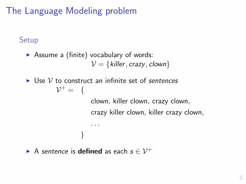
The Language Modeling problem
Setup
I Assume a (finite) vocabulary of words:V = {killer , crazy , clown}
I Use V to construct an infinite set of sentencesV+ = {
clown, killer clown, crazy clown,
crazy killer clown, killer crazy clown,
. . .
}
I A sentence is defined as each s ∈ V+
3
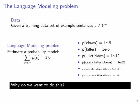
The Language Modeling problem
DataGiven a training data set of example sentences s ∈ V+
Language Modeling problem
Estimate a probability model:∑s∈V+
p(s) = 1.0
I p(clown) = 1e-5
I p(killer) = 1e-6
I p(killer clown) = 1e-12
I p(crazy killer clown) = 1e-21
I p(crazy killer clown killer) = 1e-110
I p(crazy clown killer killer) = 1e-127
Why do we want to do this?
4
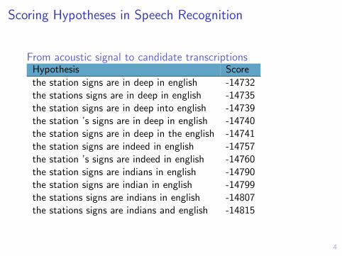
Scoring Hypotheses in Speech Recognition
From acoustic signal to candidate transcriptionsHypothesis Score
the station signs are in deep in english -14732the stations signs are in deep in english -14735the station signs are in deep into english -14739the station ’s signs are in deep in english -14740the station signs are in deep in the english -14741the station signs are indeed in english -14757the station ’s signs are indeed in english -14760the station signs are indians in english -14790the station signs are indian in english -14799the stations signs are indians in english -14807the stations signs are indians and english -14815
5
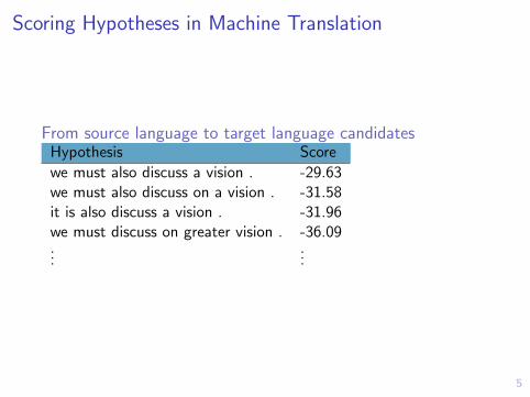
Scoring Hypotheses in Machine Translation
From source language to target language candidatesHypothesis Score
we must also discuss a vision . -29.63we must also discuss on a vision . -31.58it is also discuss a vision . -31.96we must discuss on greater vision . -36.09...
...
6
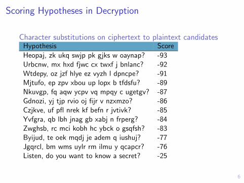
Scoring Hypotheses in Decryption
Character substitutions on ciphertext to plaintext candidatesHypothesis Score
Heopaj, zk ukq swjp pk gjks w oaynap? -93Urbcnw, mx hxd fjwc cx twxf j bnlanc? -92Wtdepy, oz jzf hlye ez vyzh l dpncpe? -91Mjtufo, ep zpv xbou up lopx b tfdsfu? -89Nkuvgp, fq aqw ycpv vq mpqy c ugetgv? -87Gdnozi, yj tjp rvio oj fijr v nzxmzo? -86Czjkve, uf pfl nrek kf befn r jvtivk? -85Yvfgra, qb lbh jnag gb xabj n frperg? -84Zwghsb, rc mci kobh hc ybck o gsqfsh? -83Byijud, te oek mqdj je adem q iushuj? -77Jgqrcl, bm wms uylr rm ilmu y qcapcr? -76Listen, do you want to know a secret? -25
7
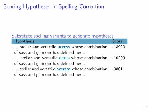
Scoring Hypotheses in Spelling Correction
Substitute spelling variants to generate hypothesesHypothesis Score
... stellar and versatile acress whose combinationof sass and glamour has defined her ...
-18920
... stellar and versatile acres whose combinationof sass and glamour has defined her ...
-10209
... stellar and versatile actress whose combinationof sass and glamour has defined her ...
-9801
8
Probability models of language
Question
I Given a finite vocabulary set VI We want to build a probability model P(s) for all s ∈ V+
I But we want to consider sentences s of each length `separately.
I Write down a new model over V+ such that P(s | `) is in themodel
I And the model should be equal to∑
s∈V+ P(s).
I Write down the model ∑s∈V+
P(s) = . . .
9
Natural Language Processing
Anoop Sarkaranoopsarkar.github.io/nlp-class
Simon Fraser University
Part 2: n-grams for Language Modeling
10
Language models
n-grams for Language ModelingHandling Unknown Tokens
Smoothing n-gram ModelsSmoothing Counts
Add-one SmoothingAdditive SmoothingInterpolation: Jelinek-Mercer Smoothing
Backoff Smoothing with DiscountingBackoff Smoothing with Discounting
Evaluating Language Models
Event Space for n-gram Models
11
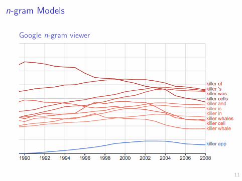
n-gram Models
Google n-gram viewer
12
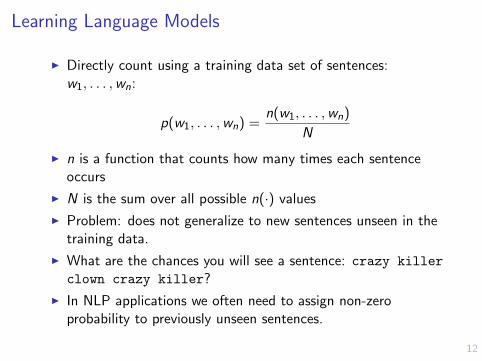
Learning Language Models
I Directly count using a training data set of sentences:w1, . . . ,wn:
p(w1, . . . ,wn) =n(w1, . . . ,wn)
N
I n is a function that counts how many times each sentenceoccurs
I N is the sum over all possible n(·) values
I Problem: does not generalize to new sentences unseen in thetraining data.
I What are the chances you will see a sentence: crazy killer
clown crazy killer?
I In NLP applications we often need to assign non-zeroprobability to previously unseen sentences.
13
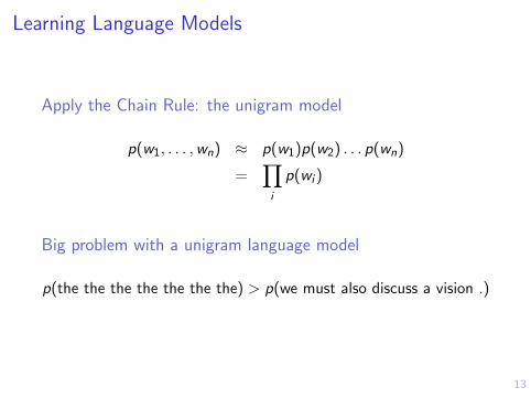
Learning Language Models
Apply the Chain Rule: the unigram model
p(w1, . . . ,wn) ≈ p(w1)p(w2) . . . p(wn)
=∏i
p(wi )
Big problem with a unigram language model
p(the the the the the the the) > p(we must also discuss a vision .)
14
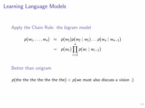
Learning Language Models
Apply the Chain Rule: the bigram model
p(w1, . . . ,wn) ≈ p(w1)p(w2 | w1) . . . p(wn | wn−1)
= p(w1)n∏
i=2
p(wi | wi−1)
Better than unigram
p(the the the the the the the) < p(we must also discuss a vision .)
15
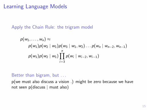
Learning Language Models
Apply the Chain Rule: the trigram model
p(w1, . . . ,wn) ≈p(w1)p(w2 | w1)p(w3 | w1,w2) . . . p(wn | wn−2,wn−1)
p(w1)p(w2 | w1)n∏
i=3
p(wi | wi−2,wi−1)
Better than bigram, but . . .
p(we must also discuss a vision .) might be zero because we havenot seen p(discuss | must also)
16
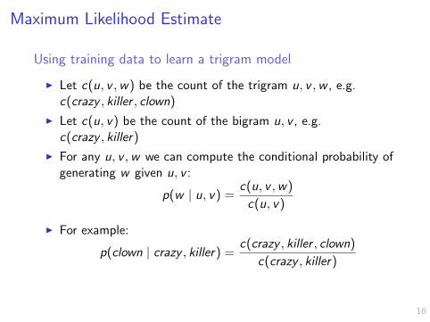
Maximum Likelihood Estimate
Using training data to learn a trigram model
I Let c(u, v ,w) be the count of the trigram u, v ,w , e.g.c(crazy , killer , clown)
I Let c(u, v) be the count of the bigram u, v , e.g.c(crazy , killer)
I For any u, v ,w we can compute the conditional probability ofgenerating w given u, v :
p(w | u, v) =c(u, v ,w)
c(u, v)
I For example:
p(clown | crazy , killer) =c(crazy , killer , clown)
c(crazy , killer)
17
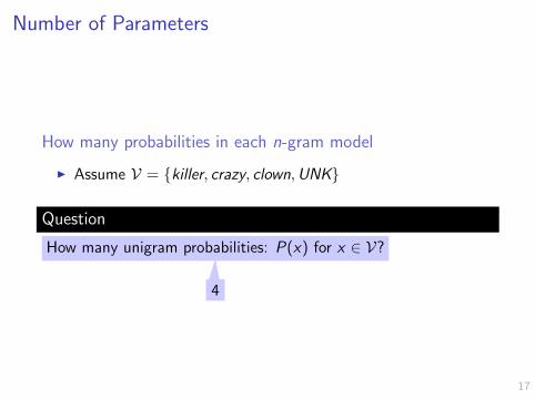
Number of Parameters
How many probabilities in each n-gram model
I Assume V = {killer, crazy, clown,UNK}
Question
How many unigram probabilities: P(x) for x ∈ V?
4
18
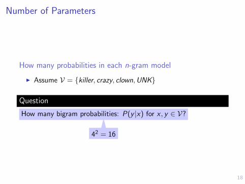
Number of Parameters
How many probabilities in each n-gram model
I Assume V = {killer, crazy, clown,UNK}
Question
How many bigram probabilities: P(y |x) for x , y ∈ V?
42 = 16
19
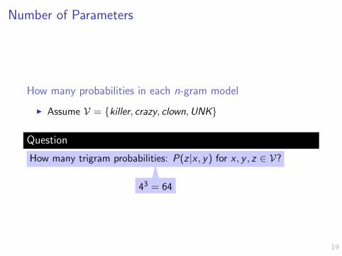
Number of Parameters
How many probabilities in each n-gram model
I Assume V = {killer, crazy, clown,UNK}
Question
How many trigram probabilities: P(z |x , y) for x , y , z ∈ V?
43 = 64
20
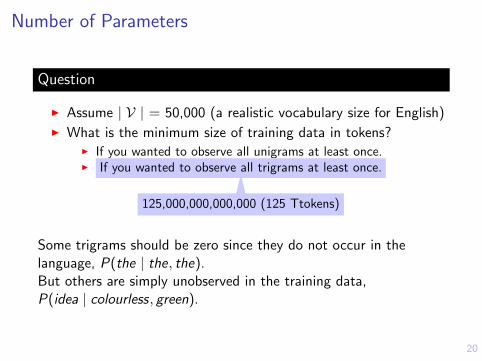
Number of Parameters
Question
I Assume | V | = 50,000 (a realistic vocabulary size for English)I What is the minimum size of training data in tokens?
I If you wanted to observe all unigrams at least once.I If you wanted to observe all trigrams at least once.
125,000,000,000,000 (125 Ttokens)
Some trigrams should be zero since they do not occur in thelanguage, P(the | the, the).But others are simply unobserved in the training data,P(idea | colourless, green).
21
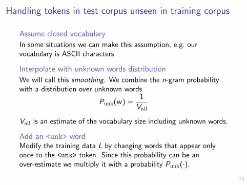
Handling tokens in test corpus unseen in training corpus
Assume closed vocabulary
In some situations we can make this assumption, e.g. ourvocabulary is ASCII characters
Interpolate with unknown words distribution
We will call this smoothing. We combine the n-gram probabilitywith a distribution over unknown words
Punk(w) =1
Vall
Vall is an estimate of the vocabulary size including unknown words.
Add an <unk> wordModify the training data L by changing words that appear onlyonce to the <unk> token. Since this probability can be anover-estimate we multiply it with a probability Punk(·).
22
Natural Language Processing
Anoop Sarkaranoopsarkar.github.io/nlp-class
Simon Fraser University
Part 3: Smoothing Probability Models
23
Language models
n-grams for Language ModelingHandling Unknown Tokens
Smoothing n-gram ModelsSmoothing Counts
Add-one SmoothingAdditive SmoothingInterpolation: Jelinek-Mercer Smoothing
Backoff Smoothing with DiscountingBackoff Smoothing with Discounting
Evaluating Language Models
Event Space for n-gram Models
24
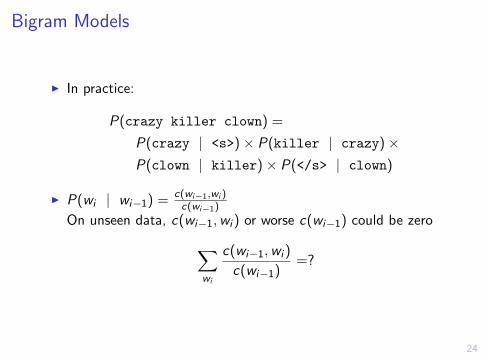
Bigram Models
I In practice:
P(crazy killer clown) =
P(crazy | <s>)× P(killer | crazy)×P(clown | killer)× P(</s> | clown)
I P(wi | wi−1) =c(wi−1,wi )c(wi−1)
On unseen data, c(wi−1,wi ) or worse c(wi−1) could be zero∑wi
c(wi−1,wi )
c(wi−1)=?
25
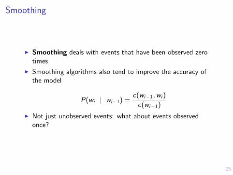
Smoothing
I Smoothing deals with events that have been observed zerotimes
I Smoothing algorithms also tend to improve the accuracy ofthe model
P(wi | wi−1) =c(wi−1,wi )
c(wi−1)
I Not just unobserved events: what about events observedonce?
26
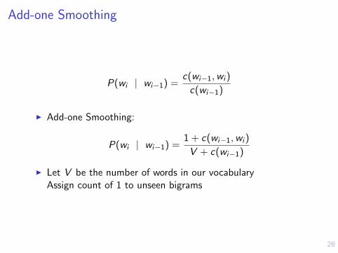
Add-one Smoothing
P(wi | wi−1) =c(wi−1,wi )
c(wi−1)
I Add-one Smoothing:
P(wi | wi−1) =1 + c(wi−1,wi )
V + c(wi−1)
I Let V be the number of words in our vocabularyAssign count of 1 to unseen bigrams
27
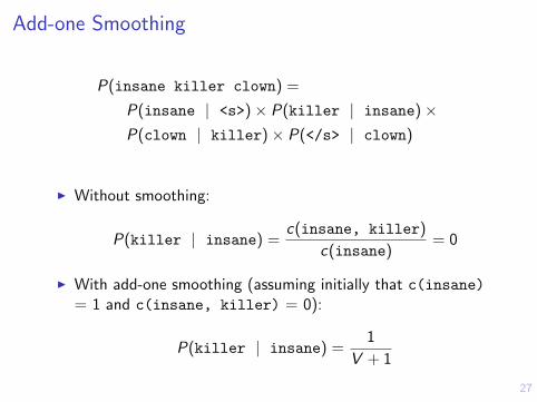
Add-one Smoothing
P(insane killer clown) =
P(insane | <s>)× P(killer | insane)×P(clown | killer)× P(</s> | clown)
I Without smoothing:
P(killer | insane) =c(insane, killer)
c(insane)= 0
I With add-one smoothing (assuming initially that c(insane)= 1 and c(insane, killer) = 0):
P(killer | insane) =1
V + 1
28
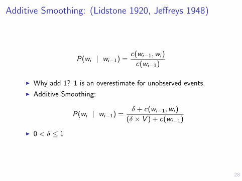
Additive Smoothing: (Lidstone 1920, Jeffreys 1948)
P(wi | wi−1) =c(wi−1,wi )
c(wi−1)
I Why add 1? 1 is an overestimate for unobserved events.
I Additive Smoothing:
P(wi | wi−1) =δ + c(wi−1,wi )
(δ × V ) + c(wi−1)
I 0 < δ ≤ 1
29
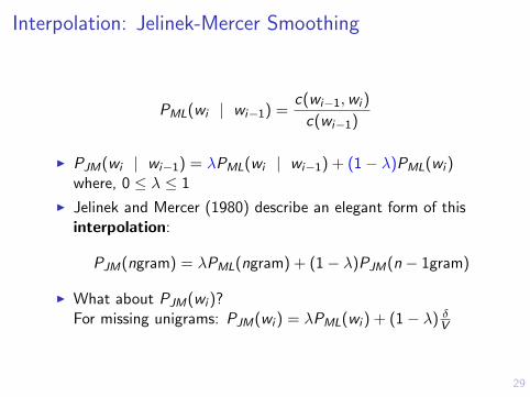
Interpolation: Jelinek-Mercer Smoothing
PML(wi | wi−1) =c(wi−1,wi )
c(wi−1)
I PJM(wi | wi−1) = λPML(wi | wi−1) + (1− λ)PML(wi )where, 0 ≤ λ ≤ 1
I Jelinek and Mercer (1980) describe an elegant form of thisinterpolation:
PJM(ngram) = λPML(ngram) + (1− λ)PJM(n − 1gram)
I What about PJM(wi )?For missing unigrams: PJM(wi ) = λPML(wi ) + (1− λ) δV
30
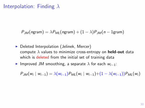
Interpolation: Finding λ
PJM(ngram) = λPML(ngram) + (1− λ)PJM(n − 1gram)
I Deleted Interpolation (Jelinek, Mercer)compute λ values to minimize cross-entropy on held-out datawhich is deleted from the initial set of training data
I Improved JM smoothing, a separate λ for each wi−1:
PJM(wi | wi−1) = λ(wi−1)PML(wi | wi−1)+(1− λ(wi−1))PML(wi )
31
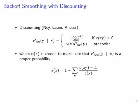
Backoff Smoothing with Discounting
I Discounting (Ney, Essen, Kneser)
Pabs(y | x) =
{c(xy)−D
c(x) if c(xy) > 0
α(x)Pabs(y) otherwise
I where α(x) is chosen to make sure that Pkatz(y | x) is aproper probability
α(x) = 1−∑y
c(xy)− D
c(x)
32
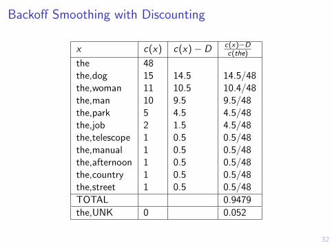
Backoff Smoothing with Discounting
x c(x) c(x)− D c(x)−Dc(the)
the 48the,dog 15 14.5 14.5/48the,woman 11 10.5 10.4/48the,man 10 9.5 9.5/48the,park 5 4.5 4.5/48the,job 2 1.5 4.5/48the,telescope 1 0.5 0.5/48the,manual 1 0.5 0.5/48the,afternoon 1 0.5 0.5/48the,country 1 0.5 0.5/48the,street 1 0.5 0.5/48
TOTAL 0.9479
the,UNK 0 0.052
33
Natural Language Processing
Anoop Sarkaranoopsarkar.github.io/nlp-class
Simon Fraser University
Part 4: Evaluating Language Models
34
Language models
n-grams for Language ModelingHandling Unknown Tokens
Smoothing n-gram ModelsSmoothing Counts
Add-one SmoothingAdditive SmoothingInterpolation: Jelinek-Mercer Smoothing
Backoff Smoothing with DiscountingBackoff Smoothing with Discounting
Evaluating Language Models
Event Space for n-gram Models
35
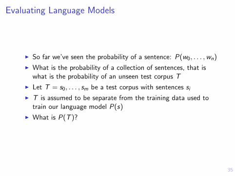
Evaluating Language Models
I So far we’ve seen the probability of a sentence: P(w0, . . . ,wn)
I What is the probability of a collection of sentences, that iswhat is the probability of an unseen test corpus T
I Let T = s0, . . . , sm be a test corpus with sentences siI T is assumed to be separate from the training data used to
train our language model P(s)
I What is P(T )?
36
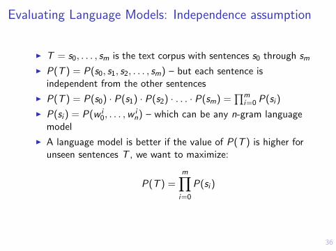
Evaluating Language Models: Independence assumption
I T = s0, . . . , sm is the text corpus with sentences s0 through smI P(T ) = P(s0, s1, s2, . . . , sm) – but each sentence is
independent from the other sentences
I P(T ) = P(s0) · P(s1) · P(s2) · . . . · P(sm) =∏m
i=0 P(si )
I P(si ) = P(w i0, . . . ,w
in) – which can be any n-gram language
model
I A language model is better if the value of P(T ) is higher forunseen sentences T , we want to maximize:
P(T ) =m∏i=0
P(si )
37
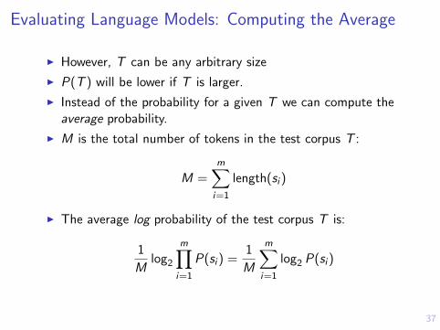
Evaluating Language Models: Computing the Average
I However, T can be any arbitrary size
I P(T ) will be lower if T is larger.
I Instead of the probability for a given T we can compute theaverage probability.
I M is the total number of tokens in the test corpus T :
M =m∑i=1
length(si )
I The average log probability of the test corpus T is:
1
Mlog2
m∏i=1
P(si ) =1
M
m∑i=1
log2 P(si )
38
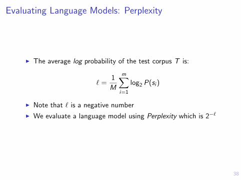
Evaluating Language Models: Perplexity
I The average log probability of the test corpus T is:
` =1
M
m∑i=1
log2 P(si )
I Note that ` is a negative number
I We evaluate a language model using Perplexity which is 2−`
39
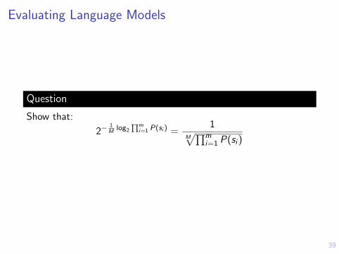
Evaluating Language Models
Question
Show that:
2−1M
log2∏m
i=1 P(si ) =1
M√∏m
i=1 P(si )
40
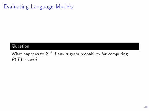
Evaluating Language Models
Question
What happens to 2−` if any n-gram probability for computingP(T ) is zero?
41
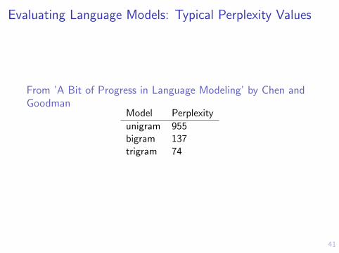
Evaluating Language Models: Typical Perplexity Values
From ’A Bit of Progress in Language Modeling’ by Chen andGoodman
Model Perplexity
unigram 955bigram 137trigram 74
42
Natural Language Processing
Anoop Sarkaranoopsarkar.github.io/nlp-class
Simon Fraser University
Part 5: Event space in Language Models
43
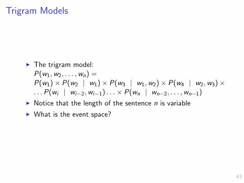
Trigram Models
I The trigram model:P(w1,w2, . . . ,wn) =P(w1)× P(w2 | w1)× P(w3 | w1,w2)× P(w4 | w2,w3)×. . .P(wi | wi−2,wi−1) . . .× P(wn | wn−2, . . . ,wn−1)
I Notice that the length of the sentence n is variable
I What is the event space?
44
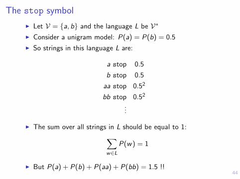
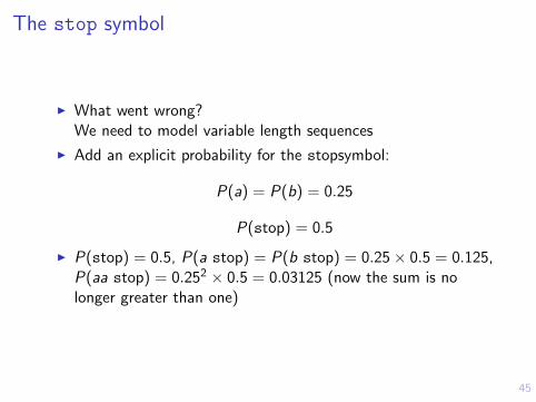
The stop symbol
I Let V = {a, b} and the language L be V∗
I Consider a unigram model: P(a) = P(b) = 0.5
I So strings in this language L are:
a stop 0.5
b stop 0.5
aa stop 0.52
bb stop 0.52
...
I The sum over all strings in L should be equal to 1:∑w∈L
P(w) = 1
I But P(a) + P(b) + P(aa) + P(bb) = 1.5 !!
45
The stop symbol
I What went wrong?We need to model variable length sequences
I Add an explicit probability for the stopsymbol:
P(a) = P(b) = 0.25
P(stop) = 0.5
I P(stop) = 0.5, P(a stop) = P(b stop) = 0.25× 0.5 = 0.125,P(aa stop) = 0.252 × 0.5 = 0.03125 (now the sum is nolonger greater than one)
46
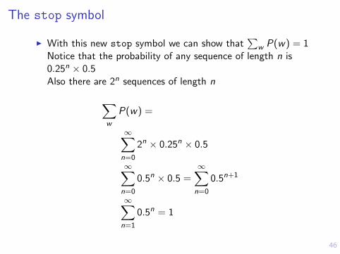
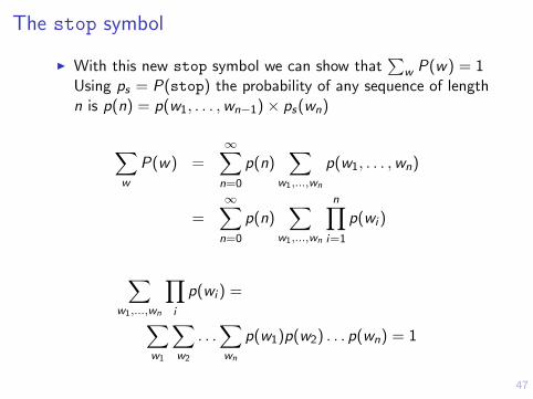
The stop symbol
I With this new stop symbol we can show that∑
w P(w) = 1Notice that the probability of any sequence of length n is0.25n × 0.5Also there are 2n sequences of length n
∑w
P(w) =
∞∑n=0
2n × 0.25n × 0.5
∞∑n=0
0.5n × 0.5 =∞∑n=0
0.5n+1
∞∑n=1
0.5n = 1
47
The stop symbol
I With this new stop symbol we can show that∑
w P(w) = 1Using ps = P(stop) the probability of any sequence of lengthn is p(n) = p(w1, . . . ,wn−1)× ps(wn)
∑w
P(w) =∞∑n=0
p(n)∑
w1,...,wn
p(w1, . . . ,wn)
=∞∑n=0
p(n)∑
w1,...,wn
n∏i=1
p(wi )
∑w1,...,wn
∏i
p(wi ) =∑w1
∑w2
. . .∑wn
p(w1)p(w2) . . . p(wn) = 1
48
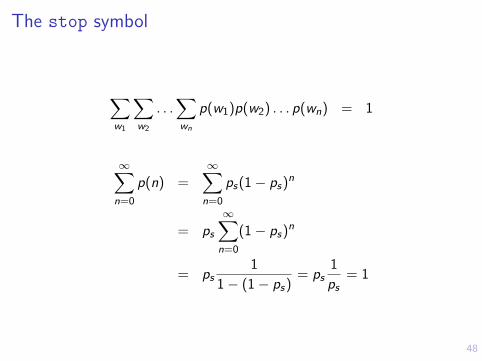
The stop symbol
∑w1
∑w2
. . .∑wn
p(w1)p(w2) . . . p(wn) = 1
∞∑n=0
p(n) =∞∑n=0
ps(1− ps)n
= ps
∞∑n=0
(1− ps)n
= ps1
1− (1− ps)= ps
1
ps= 1
49
Acknowledgements
Many slides borrowed or inspired from lecture notes by MichaelCollins, Chris Dyer, Kevin Knight, Philipp Koehn, Adam Lopez,Graham Neubig and Luke Zettlemoyer from their NLP coursematerials.
All mistakes are my own.
A big thank you to all the students who read through these notesand helped me improve them.