Natural Gas Engineering Dr.B. Pankaj Tiwari Department of...
17
Natural Gas Engineering Dr.B. Pankaj Tiwari Department of Chemical Engineering Indian Institute of Technology – Guwahati Module No # 01 Lecture No # 03 Introduction to Natural Gas – III Hello everyone we are still in the week one introduction to natural gas this is third lecture on introduction to natural gas. (Refer Slide Time: 00:40) In this lecture we are going to understand some of the mathematical techniques those will be using and we go further in our class. So let us revise what we studies in second natural gas introduction class we had discussed about the phase diagram in detail. We started with component 1 when only one component is present we are having the phase behavior means PVT diagram and specifically PT diagram when we are changing temperature and pressure condition how component can go to vapor phase to liquid phase and liquid phase to vapor phase. The line that represent the separation is called the vapor pressure line and the dew point and bubble point both are same when the component single component is present in the system. We extended our discussion to two component system or multi component system or
Transcript of Natural Gas Engineering Dr.B. Pankaj Tiwari Department of...

Natural Gas EngineeringDr.B. Pankaj Tiwari
Department of Chemical EngineeringIndian Institute of Technology – Guwahati
Module No # 01Lecture No # 03
Introduction to Natural Gas – III
Hello everyone we are still in the week one introduction to natural gas this is third lecture on
introduction to natural gas.
(Refer Slide Time: 00:40)
In this lecture we are going to understand some of the mathematical techniques those will be
using and we go further in our class. So let us revise what we studies in second natural gas
introduction class we had discussed about the phase diagram in detail. We started with
component 1 when only one component is present we are having the phase behavior means
PVT diagram and specifically PT diagram when we are changing temperature and pressure
condition how component can go to vapor phase to liquid phase and liquid phase to vapor
phase.
The line that represent the separation is called the vapor pressure line and the dew point and
bubble point both are same when the component single component is present in the system.
We extended our discussion to two component system or multi component system or

specifically for hydro carbon mixture or system of multi component system compose of
several hydro carbon components.
In that discussion we had understanding of when the mixture is consider for phase behavior
study or specifically on PT diagram it creates an envelope. And that envelope is having
bubble line bubble point curve on one side and the dew point curve on the second type and
both the sides of the envelope they just concede at the point that is called the critical point
compared to single point critical point in multicomponent system is not the highest
temperature or highest pressure point.
Highest temperature point where only the beyond that only the gas will be available or the
system will be only in the gas phase is called cricondentherm. Similar for the pressure when
the system above that pressure will always be on the liquid phase irrespective of the
temperature.
We understand criconderbar and concondentherm we also understand how to classify the
reservoir based on the phase diagram that depends on the composition of the gas or the fluid
being produced at what condition means reservoir condition and surface condition the fluid
is being considered the shape of this envelope will depend on the composition if we are
having the different composition of the mixture the shape will be different.
Based on that we can classify where what shape this particular envelope is taking it is going to a
liquid side or more towards the vapor side if we consider the fluid is at a reservoir condition.
Our case is more specifically towards the natural gas. So natural gas reservoir are classified
as dry, wet and condensate it means initially the reservoir pressure is somewhere here that is
beyond the crecondentherm temperature.
The reservoir condition are here so for example if it is here point A this is a gas reservoir because
the temperature is beyond cricondentherm temperature and we are isothermally reducing the
pressure we are always getting the gas phase only but there might be situation when it is
entering in the two phase system we will be having the wet system or wet gas system.

Then will be a situation when the initial reservoir temperature and pressure or somewhere here or
specifically the temperature is between critical point and cricondemtherm. If this is the
situation isothermally we are reducing the temperature this system will pass through several
quality lines and those quality lines will say the phase change is happening the gas is going
to liquid or some part of the gas is going to liquid when it is entering in the envelope and
further reducing the pressure the liquid is getting re-vaporized.
This behavior is reversible compared to single compound represent that is why it is called as
retrograde behavior and it produces liquid at this surface facility or during the when the
pressure is reaching within this envelope condition we called it retrograde condensate gas
reservoir. If the condition are very near to very critical point it will pass through several
quality lines it means the system will be changing it composition very frequently from gas
phase to liquid phase, liquid phase to gas phase.
And when this is happening this will be very complex phenomena to understand when exactly
the pressure and temperature are going to affect the composition and how the fluid is going
to change from gas phase to liquid phase and from the liquid phase to gas phase. The
problem comes when the phase change is happening near the wellbore region near the
region the liquid is getting accumulated the liquid which comes out or dropped out from the
gas phase is getting accumulated reducing the permeability for the gas ceasing the
production of gas and create a problem.
Similar may happen in the pipeline where the pressure and temperature are reaching up to certain
point when the liquid is coming out from the gas phase and chocking the wellbore or
creating certain different type of two phase flow system where it is required to understand
how to deal with this kind of problem and this problem called the liquid loading problem.
All this understanding of phase behavior change when the fluid is travelling from reservoir to
surface different temperature and pressure zone how it is changing the phase is very
important to apply the proper mechanism how to control the production? How to control
liquid production that is being produced from a gas reservoir is very important also
important for the prediction of production behavior in the future.

This also very important when we are designing the surface facilities especially the separator
when this fluid is coming to the surface it is going to be in a dry gas like this kind of the A
point it is going to be a bad gas when it is entering in this region phase envelope and it is
going to be a condensate or retrograde condensate type of fluid where we are having sudden
change of from vapor to liquid, liquid to vapor when we are changing the pressure.
That is because very important we will discuss in the class of separator when this condensation
happen or retrograde condensation behavior happens certain mechanism can be applied
based on experience based on the understanding of compressive understanding of the
reservoir this tells us or provide us certain guidelines how to take appropriate measurement
appropriate action to avoid the ceasing of production sometimes recovering the valuable
production like the liquid that is more valuable than the gas we are not leaving them in the
reservoir itself.
That can be done by having the gas cycling is whatever the gas is being produced on the surface
can be re-injected in the well and that will change the composition of the fluid with in the
reservoir domain or in wellbore that will allow to come allow the liquid to come out to
surface with the gas other could be injecting some solvent those could be gaseous or liquid
solvent those allowing the liquid to come out to surface or artificial lift mechanism also be
applied.
So with this understand we can say if we are having the understanding of phase behavior from
the reservoir temperature pressure to surface temperature and pressure we can classify the
system or the production well at the separator are based on the GOR gas to oil ratio what
type of reservoir it is it can also be understood with the help of degree API of liquid it is
producing for example the dry gas reservoir will produce more liquid wet gas will be having
some very transparent liquid and condensate will be having fluid of around 45 degree API.
(Refer Slide Time: 08:58)

So GOR, API and color can also distinguish what type of the reservoir gas reservoir it is with this
I would like to introduce you some of the techniques those we are going to use very
frequently when we are dealing with the natural gas classes. The need of the technique will
start from the beginning itself and we are understanding how to calculate the properties of
the natural gas how the natural gas is being produced how we are treating the natural gas at
the end how we are transporting this natural gas to consumer.
Some mathematical tools are required to solve the mathematical expression those represent each
of this phenomena. So one of the technique is trapezoidal rule this is to integrate any
function which are going to get in your complex system of mathematical equation being
system is very complex because the properties are function of composition and when
composition are changing our properties will get change properties are changing certain
parameters we will get in and when this parameter are changing the behavior or nature of the
mathematical equation those are present in particular phenomena for example IPR, WPR
and CPR or any other will also get affected.
So the trapezoidal rule is a technique for approximating the definite integral and in this
techniques the area under the curve is measured for example we are having this kind of the
function fx that supposed to be integrated from a to b with respect to x. So fx is the integral a
is the lower limit of integration b is the upper limit of integration if the function is very

simple like we can integrate analytically we can do that putting the limit we will get the
answer or we will get how what is the area under this curve.
For example if it is represented by fx what is the area under this curve can be easily calculated if
this function fx is having analytical solution very simple solution certain cases when the
analytical solution either very complex or not available we can still integrate that thing.
In that case what we can do we can use trapezoidal kind of the rules or there are several
integration process trapezoidal is one of them and one of the simplest among the we can
integrate considering the trapezoidal shape of the curve we can use this formula that says
area under this curve can be represented by b – a function value at a + function value of b /
2.
So the average of both the function value multiple by the range over which this area is
distributed from a to b we can do this we can calculate the fe value this function value at a
we can calculate function value of b. When we are having like large area to be integrated
what we can do to improve the accuracy of the calculation we can divide this in a several
segment. For example if this area is divided in n segment and each segment is having the
width of h that is calculated by b – a / n.
n is number of the segments we are going to divide this x axis for example this is our y axis is y
fx. So what we can do we can calculate xn + 1 is next just action + x we keep adding h
increment in each and calculating the area using the same formula for that one segment
second segment and all the segment and then we can calculate the we can add up all this
segments area using the trapezoidal rule and we can say the total area under this curve can
be estimated with the help of this formula.
Where a is the approximate area of this curve equal to h is a b – a yn / 2 then we are having the
value at one point is A this is kind of F of A this is F of B and +2 all the intermediate terms
we are having should be added up and multiply by 2 and this will give us the area. You will
find the application of this trapezoidal rule at several places specifically when we are going
to discuss about one of the mathematical way of representing gas properties is called pseudo

real gas pressure that is defined as mp and that is mathematically defined as integration 2p /
Mu z dp.
Here you see we are integrating with respect to p but Mu and z both are not constant they are the
function of pressure and for such kind of system when we are integration any base pressure
to pressure of interest what we can say we can divide this pv to p in a small segment can
calculate the value of Mu and z between that small segment we can calculate the average
properties of Mu average values of z and integral submission or cumulative summation of
all this small integral will give us the value of mp at that pressure of interest.
(Refer Slide Time: 14:30)
Another technique that we are going to discuss is Newton Raphson methods you will find during
the course you will find there are several situation there are several mathematical equation
when we are having this kind of the function where x the parameter of interest which we are
supposed to calculate is a function of itself like x is appearing on the left hand as well as on
the right hand side this appears in IPR this appears in several formulas where we need to do
some iteration processor or optimization processor to find out the root of or the value of x
that satisfied this situation.
One of the simplest technique is Newton Raphson method or Newton method this method is
based on this simple idea of the linearization recursive algorithm may be adopted recursion
is we are using the new approximation based on the previous approximation whatever the

value you got in the last step you are using that value as the Mu value for the next step. So
this is a step y is a processors where attritions are performed newton Rephson can provide us
the value of x that should be used.
If it is just a simple first order system we know how to solve the equation and get the value of x
if it is a quadrating nature we can get the formula we are having even polynomial of third
order or even up to forth order we can solve it or when it is very complex in nature not
necessary it is just a polynomial it may be in the law form may the exponential form or it
may be a combination of anything in that situation having a numerical method in hand is
very good to calculate the root of that equation or value of the parameter is satisfied that
equation.
So in newton Raphson method what we do first we rearrange the equation given to us in the form
of fx = 0 take everything on the left hand side make right side 0 and we are in this situation
what we do we start solving it by choosing suitable initial gas and that initial gas is very
important because for example this is having this kind of shape when we know this
intersecting this x coordinate at r location this r is the root for this equation y = fx we want
to know the value of r means the value of x = r where this is curve this curve intersecting x
coordinate.
But we do not what that value is we can initially guess some value for example here it is x1 some
literature it is start from x0 let us say we are a x1 we are starting first iteration if the gas
value that x1 when we know x1 value we can calculate this point on the curve this is x1 fx1
this is if it is 1 this is fx1. By having the tangent principle or the tangent on that point we can
guess the Mu value xn + 1 and that xn + 1 is x2 for the first iteration that x1 + 1 = x1 – fxn /
f prime xn.
f prime xn will come and when we are trying this tangent on this point so to calculate the next
approximation what we need initial gas first condition initial gas second the function value
at initial value second take the derivative of that function f prime and evaluate the value of
the function f prime at that condition xn and if it is happening what we are going to get the
Mu value xn + 1 by using this formula.
So when we get the Mu value xn+1 we have to judge the value achieved is the desired value or
not means the value which going to satisfy the function we can judge either putting that
value in function and saying fx n + 1 is becoming 0 or not means it is a root of that
polynomial or the function fx or not other way could be calculating in terms of the absolute
relative approximation error that says if the error is 2.00 this up to the decimal point dew on
we can stop otherwise we have to repeat.
So acceptable then end otherwise next step simply says xn next xn = xn + 1 this is somewhere xn
+ 1. After replacing this we are again here we can calculate the value at the next step and we
can keep doing this we are approaching more towards our solution so we started from xn we
are moving towards r and when we value is acceptable when the function value fx is 0 up to
the decimal point we want we are ok and we can say this the solutions of the equation of the
residue value of x that is to satisfy that equation.
As I said this is going to be face several time in our natural gas class so better let us understand
this for more time with the help of an example.
(Refer Slide Time: 20:11)
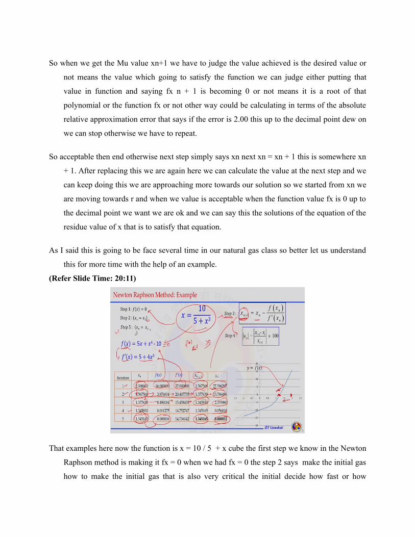
That examples here now the function is x = 10 / 5 + x cube the first step we know in the Newton
Raphson method is making it fx = 0 when we had fx = 0 the step 2 says make the initial gas
how to make the initial gas that is also very critical the initial decide how fast or how

accurate you are going to achieve the actual root or real root of the real function that can be
done by putting few values of x and saying when it is coming negative is lesser than 0 and
when it is greater than 0 we can take one when if it is the situation.
When it is one condition it is negative another condition is positive we can say the value of root
between these two limits and we can take positive side and start the calculation. For example
in this case we are going to assume one value once we assume that value based on certain
understanding how to choose the initial gas we can go to next step third and step third is
calculate the Mu value because the value is you had in your hand for xn that is assume value
may not be correct.
So for the next round we have to go xn + 1 that says use this formula xn-fxn / fx prime xn you
will get xn + 1. Once you get this fourth step calculate the error if satisfy it is ok otherwise
go to step 5 replace the value put it in the recursive mode go back to step 3 and start doing
this thing. So the example which I had chosen is if we rearrange this it will like fx = 5x + x
to the power of 4 – 10 simple and that is equal to 0.
Now the job is how to find out the value of x that is going to satisfy this expression fx now we
can calculate f prime x is also that is 5 + 4x cube. So the newton Raphson method depends
on the function we are having can be derivate can be go through under the derivative or not.
So we got this f prime x 5 + 4x cube let us begin either write mathematical code in some
mathematical language or just can just go do work in the work sheet excel or some other.
So let us say here we did work in the MS office excel where iteration 1 says initial gas that I had
chosen 2 put up to certain decimal point for the accuracy to at that xnI calculated fx and f
prime x because I already know how to put the value of xn and calculate those function fx as
well as f prime x. Now the Mu value xn + 1 I can use this formula I got to the xn + 1 next is
calculate the error when I calculate the absolute error it came out as 27 not acceptable of
course.
We have to go to next step two this value xn + 1 should come here and when it is xn become
1.567 certain decimal points we have to calculate again fx, f prime x and process like this
only you will get xn + 1 again calculate the error it is ok no we can go back to iteration
number 3 where x3 is from the previous calculation xn + 1 is this x this valve it come here
similar calculation for fx, f prime x we are going to get Mu value of xn + 1 and error is still
significant high to 2 point something.
We are going to forth iteration when we are going to do fourth iteration more it came out error is
0.05% if you are satisfy you can stop here if you want more accurate result we can go to
another steps and that an another steps is the value of function at that point is 0.000006 that
means we almost find the root of the equation that satisfy it up to decimal five decimal point
and the error is also very low that is why we can terminate our iteration and can say the
value of x is 1.345165 is the root of the equation that we are solving.
Here we can see the from picture also this is the functionality for this y = fx initial gas we had
taken around this 2 and from 2 we moved further and fourth fifth iteration we reach a point
where it is intersecting this and the value came out is 1.345 this is very simple technique and
it will be very required when we are solving several numerical problems of natural gas
engineering.
(Refer Slide Time: 25:51)
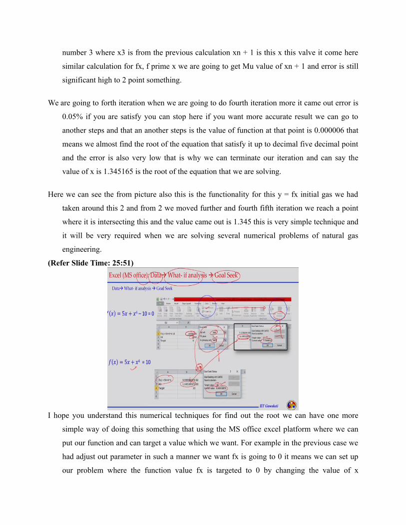
I hope you understand this numerical techniques for find out the root we can have one more
simple way of doing this something that using the MS office excel platform where we can
put our function and can target a value which we want. For example in the previous case we
had adjust out parameter in such a manner we want fx is going to 0 it means we can set up
our problem where the function value fx is targeted to 0 by changing the value of x
repeatedly and that can be done if we go into MS office go to data and data what if analysis
and that is where the goal seek is.
Here I have highlighted that part it says if we go to data we will see this what if analysis mode
here you will see 2, 3 drop down one of them is goal seek you just choose the goal seek and
you will be able to get the this kind of the small window which says set cell is you can write
the expression here which I had written here in the B2 if you write that expression 5x + x to
the power 4 – 10 in this form you can just click that cell here means if you are setting cell
B2 to set value 0.
Because i want this function to be 0 and while changing the value of x0 initial gas I have taken
here very high we have chosen 13 and when I hit ok the iteration will start the X0 value will
keep changing and while changing this value of x0 the function value will be evaluated
internally and finally what we are going to get the answer is like this that says the function
value is 10 to the power – 6 this almost 0 and at that condition the value of x is 1.345164.
And if you see at this condition the target value was 0 we achieved almost 0 means up to then to
the -6 point we reach if it is 0 numerically and the value we are going to get for x is almost
same up to 4 decimal point same as what we got from the Newton Raphson method. So this
is one of the simplest convenient technique that is available in MS office you just need to
write the expression in what particular shell and that another targeted cell changing that
particular cell you are going to achieve the function value and that function value not
necessary be 0 it can be anything.
For example in second case when I adjusted this fx in such a manner 5x to the power 4 = 10 I
had written the expression here 5x + x to the power 4 and I want this function is getting
converted to 10 by changing the value x. Similar I will go to data from data I will go to what
if analysis and from what if analysis we will get this window similar window here I will set
again B2 set value now I will change my set value is 10.
So it ask the set cells should reach what value also it should reach the value of 10 when I am
asking this hitting ok but solution will coming out like this it says the target value was 10 the
software or the internal iteration could achieve 9.999388 something and at this condition the
value of x is 1.3451. So same equation we solve the same the value should also be same if
we compare almost up to 3, 4 decimal points the value is same.
So with the help of this goal seek in not only able to solve any function which should reach 0
value like in the Newton Raphson case we take everything on the left hand side and make
the function value = 0 but with help of goal seek you can target I want this production
pressure I want to calculate at this production pressure what is my flow rate it you do need
to take everything on the left hand side and making the function value 0 that is one of the
usefulness of this goal seek tool in the MS office.
(Refer Slide Time: 30:16)
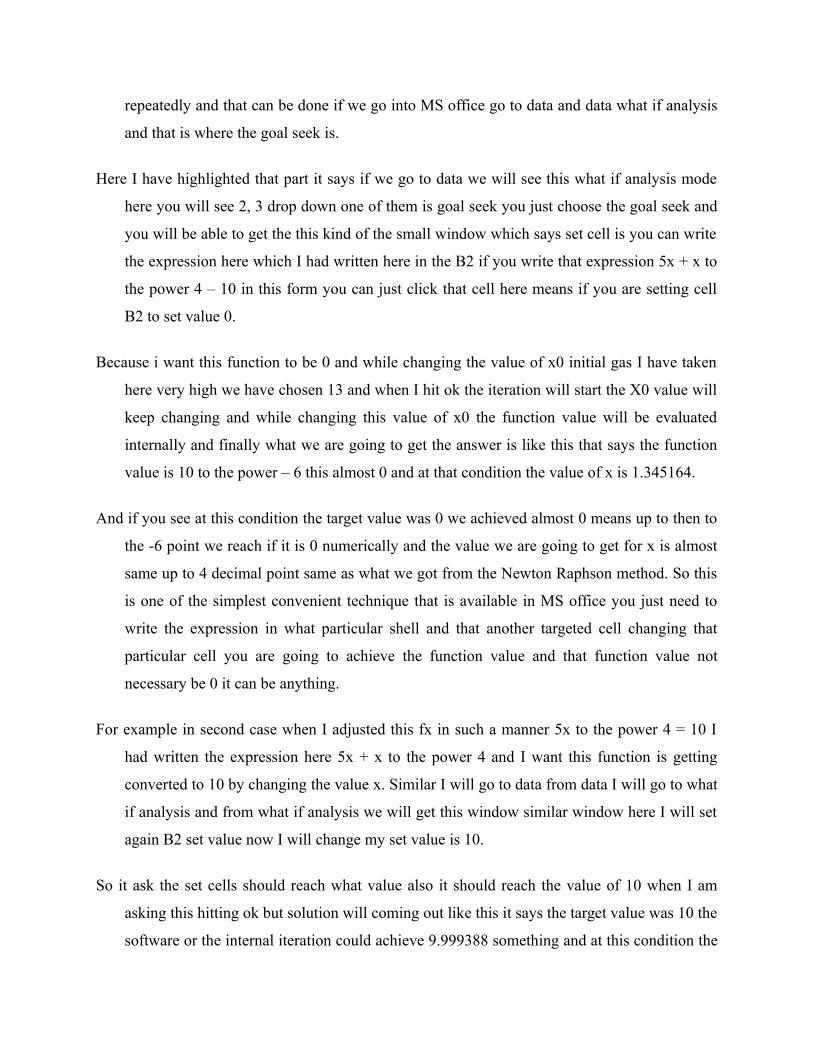
Another thing which you will frequently face in natural gas calculations or in the numerical part
having several correlation or the charts this charts are developed long time back based on
several experimental experiments mostly those are based on the experiments or the data
collected from the field experiments. For example here I am showing for viscosity it is very
complex it says how the viscosity is the function of gas gravity as well as molecular weight
and this is the temperature data.
Now corrections should be made for the impurities like in hydrogen CO2 and S2S present in that
so if you are having a gas mixture which is having the hydrocarbon and non-carbon gases
you are supposed to calculate the Viscosity even this advent atmosphere supposed to
calculate at higher pressure you have to read this chart or you have to use some correlation

those are developed out based on this chart and you will often found those correlation need
some iteration.
They need come iteration and that is why the Newton Raphson method or the Goldsmith
technique or this macros those can be written in excel will help you to solve such complex
problem. Another example could be when we are having very simple case of fluid is being
float on the pipeline and when the fluid is flowing through the pipeline if we want to
understand the behavior of the fluid we know we have to calculate the Reynolds number
because Reynolds number tells us the flow is under laminar conditions or under the
turbulent conditions.
It is very much required because the value of friction factor that appears in the energy balance
equation when we are setting up the problem for fluid flow through pipeline we see the F
value depends on the Reynolds number and based on the Reynolds number and the
roughness of the pipe or the other parameter we have to calculate the either the Moody’s
friction factor or Moody’s friction factor or finding friction factor.
To have that we have to calculate the Reynolds number and when we look Reynolds number is a
function of Q and Q is a function of temperate and pressure it becomes complex systems.
Just to read a small chart we can read that chart if we know the Reynolds number value and
the Reynolds number value depends on other parameter that is why it becomes little bit
complex problem when we deal the some real situation like the real gas system where the
properties are function of temperature and pressure and when we are going to read any chart
or any correlation that depends on the range as been chosen.
So in summary I would like to say the empirical correlation and chart will often appear in the
calculation and we have to understand how to read those chart and how to calculate the
parameter of interest using the correlation those have been developed from these chart. The
correlation may be little different because the way the chart has been read what parameter is
dependent parameters and independent parameters are chosen to represent the complexity
involved in these charts.
(Refer Slide Time: 33:49)
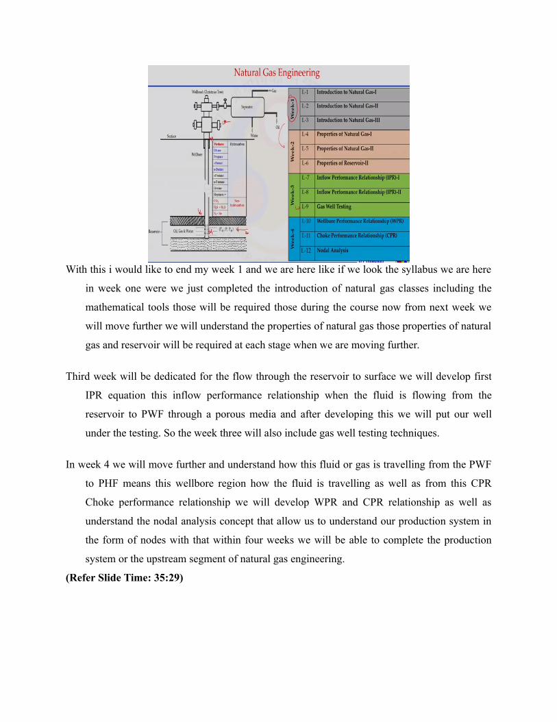
With this i would like to end my week 1 and we are here like if we look the syllabus we are here
in week one were we just completed the introduction of natural gas classes including the
mathematical tools those will be required those during the course now from next week we
will move further we will understand the properties of natural gas those properties of natural
gas and reservoir will be required at each stage when we are moving further.
Third week will be dedicated for the flow through the reservoir to surface we will develop first
IPR equation this inflow performance relationship when the fluid is flowing from the
reservoir to PWF through a porous media and after developing this we will put our well
under the testing. So the week three will also include gas well testing techniques.
In week 4 we will move further and understand how this fluid or gas is travelling from the PWF
to PHF means this wellbore region how the fluid is travelling as well as from this CPR
Choke performance relationship we will develop WPR and CPR relationship as well as
understand the nodal analysis concept that allow us to understand our production system in
the form of nodes with that within four weeks we will be able to complete the production
system or the upstream segment of natural gas engineering.
(Refer Slide Time: 35:29)

Further in week 5 we will be understanding the natural gas processing as well as the first
equipment the natural gas is going to encounter at the surface is separator we will be having
the understanding of separator as well as separator design further moving we will refer our
natural gas by using the dehydration and sweeting process. So week 7 will be on the
measurement of natural gas as well as transportation of natural gas from surface facility
consumer in the form of either LNG or CNG or through the pipeline the special focus will
be on pipeline design.
In the final week we will discuss some of the source those we encounter in the natural gas
conventional natural gas production as well as we will dedicate some time to understand the
unconventional natural gas resources and finally it will be a review class that is where I will
summarizing all the content of this course. If you see here more number of lecturers are
appearing so it may happens some of the lectures are getting merged. For example the
special resource be natural gas production may be merge with transportation of natural gas
class.
Similarly here the measurement of natural may get merged with the compressor design so there
may be a slightly change in the structure of the lectures but altogether it will be twenty hours
lecture and we will try to understand all the aspects or we will cover all the aspect of the
natural gas production system.
(Refer Slide Time: 37:11)
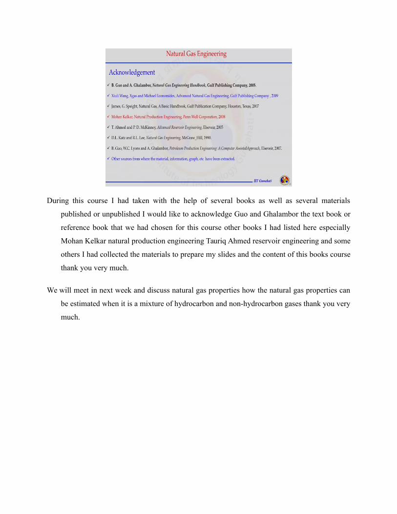
During this course I had taken with the help of several books as well as several materials
published or unpublished I would like to acknowledge Guo and Ghalambor the text book or
reference book that we had chosen for this course other books I had listed here especially
Mohan Kelkar natural production engineering Tauriq Ahmed reservoir engineering and some
others I had collected the materials to prepare my slides and the content of this books course
thank you very much.
We will meet in next week and discuss natural gas properties how the natural gas properties can
be estimated when it is a mixture of hydrocarbon and non-hydrocarbon gases thank you very
much.