Natural frequency of Cobiax flat slabs Lukas Wolskiirancobiax.com/f/web/520354458021.pdf · Natural...
112
Natural frequency of Cobiax ® flat slabs Lukas Wolski Thesis submitted in partial fulfilment of the requirements for MSc in Civil and Structural Engineering Coventry University September, 2006
Transcript of Natural frequency of Cobiax flat slabs Lukas Wolskiirancobiax.com/f/web/520354458021.pdf · Natural...
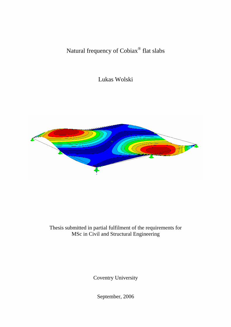
Natural frequency of Cobiax® flat slabs
Lukas Wolski
Thesis submitted in partial fulfilment of the requirements for MSc in Civil and Structural Engineering
Coventry University
September, 2006
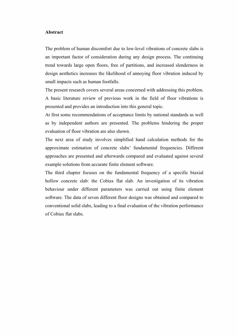
Abstract
The problem of human discomfort due to low-level vibrations of concrete slabs is
an important factor of consideration during any design process. The continuing
trend towards large open floors, free of partitions, and increased slenderness in
design aesthetics increases the likelihood of annoying floor vibration induced by
small impacts such as human footfalls.
The present research covers several areas concerned with addressing this problem.
A basic literature review of previous work in the field of floor vibrations is
presented and provides an introduction into this general topic.
At first some recommendations of acceptance limits by national standards as well
as by independent authors are presented. The problems hindering the proper
evaluation of floor vibration are also shown.
The next area of study involves simplified hand calculation methods for the
approximate estimation of concrete slabs’ fundamental frequencies. Different
approaches are presented and afterwards compared and evaluated against several
example solutions from accurate finite element software.
The third chapter focuses on the fundamental frequency of a specific biaxial
hollow concrete slab: the Cobiax flat slab. An investigation of its vibration
behaviour under different parameters was carried out using finite element
software. The data of seven different floor designs was obtained and compared to
conventional solid slabs, leading to a final evaluation of the vibration performance
of Cobiax flat slabs.

Acknowledgments
First of all I would thank my supervisor Dr. Messaoud Saidani for his support,
patience and guidance throughout the development of this thesis. Thanks are also
due to Dr John Davies and John Karadelis for their advice and their help to realise
this research.
I would like to express sincere gratitude to Prof. Dr.-Ing. Andrej Albert for his
generous support and guidance throughout this dissertation. His suggestions and
encouragement has been greatly appreciated.
Many thanks are due to Cobiax Technologies GmbH in Darmstadt, Germany and
Cobiax Technologies Ltd in London, United Kingdom. Special thanks go to
Dr. Karsten Pfeffer and Daniel Ptacek who helped to establish this project and
supported it during its completion.
I must also thank Christian Roggenbuck, for his constant support and helpful
advice not only throughout this research but for the entire last year.
Finally, I need to thank my family and especially my girlfriend for their never
ending belief in me and my ability to accomplish what I set out to do. Their
support and love have allowed me to achieve this goal.
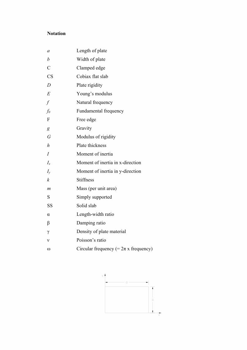
Notation
a Length of plate
b Width of plate
C Clamped edge
CS Cobiax flat slab
D Plate rigidity
E Young’s modulus
f Natural frequency
f0 Fundamental frequency
F Free edge
g Gravity
G Modulus of rigidity
h Plate thickness
I Moment of inertia
Ix Moment of inertia in x-direction
Iy Moment of inertia in y-direction
k Stiffness
m Mass (per unit area)
S Simply supported
SS Solid slab
α Length-width ratio
β Damping ratio
γ Density of plate material
ν Poisson’s ratio
ω Circular frequency (= 2π x frequency)
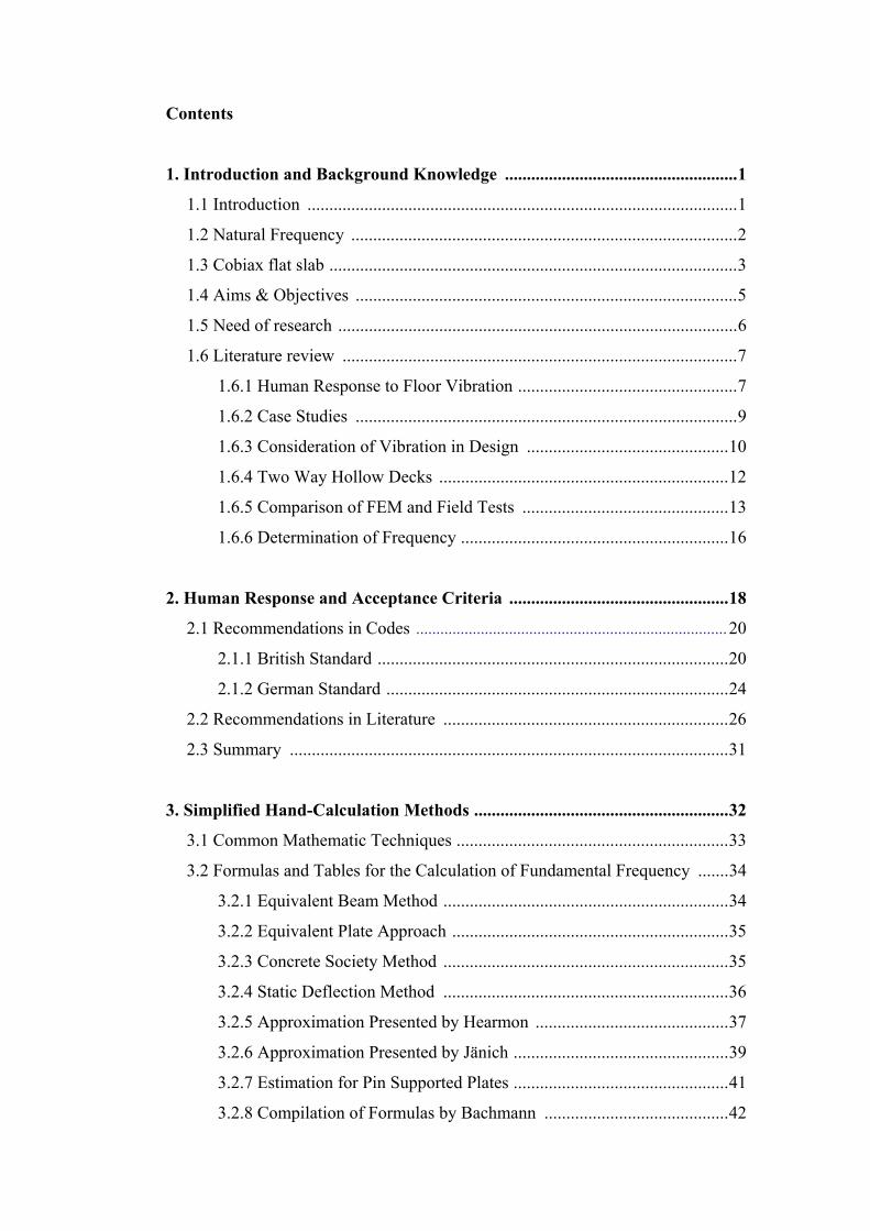
Contents
1. Introduction and Background Knowledge .....................................................1
1.1 Introduction ..................................................................................................1
1.2 Natural Frequency ........................................................................................2
1.3 Cobiax flat slab .............................................................................................3
1.4 Aims & Objectives .......................................................................................5
1.5 Need of research ...........................................................................................6
1.6 Literature review ..........................................................................................7
1.6.1 Human Response to Floor Vibration ..................................................7
1.6.2 Case Studies .......................................................................................9
1.6.3 Consideration of Vibration in Design ..............................................10
1.6.4 Two Way Hollow Decks ..................................................................12
1.6.5 Comparison of FEM and Field Tests ...............................................13
1.6.6 Determination of Frequency .............................................................16
2. Human Response and Acceptance Criteria ..................................................18
2.1 Recommendations in Codes .............................................................................20
2.1.1 British Standard ................................................................................20
2.1.2 German Standard ..............................................................................24
2.2 Recommendations in Literature .................................................................26
2.3 Summary ....................................................................................................31
3. Simplified Hand-Calculation Methods ..........................................................32
3.1 Common Mathematic Techniques ..............................................................33
3.2 Formulas and Tables for the Calculation of Fundamental Frequency .......34
3.2.1 Equivalent Beam Method .................................................................34
3.2.2 Equivalent Plate Approach ...............................................................35
3.2.3 Concrete Society Method .................................................................35
3.2.4 Static Deflection Method .................................................................36
3.2.5 Approximation Presented by Hearmon ............................................37
3.2.6 Approximation Presented by Jänich .................................................39
3.2.7 Estimation for Pin Supported Plates .................................................41
3.2.8 Compilation of Formulas by Bachmann ..........................................42
3.2.9 Compilation of Formulas by Blevins ...............................................44
3.3 Analysis of Results .....................................................................................45
3.4 Conclusion ..................................................................................................47
4. Numerical Analysis .........................................................................................48
4.1 Software ......................................................................................................49
4.2 Verification of Software Accuracy .............................................................50
4.2 General Settings .........................................................................................52
4.3 Analysis of Results .....................................................................................54
4.4 Conclusion ..................................................................................................59
5. Conclusions and Recommendations ..............................................................60
5.1 General Conclusions ...................................................................................60
5.2 Areas of Future Research ...........................................................................61
References ............................................................................................................62
APPENDIX A (Simplified Hand Calculation) ....................................................67
APPENDIX B (Calculated Values by FEM) .......................................................93
APPENDIX C (Cobiax Information) .................................................................101
Figures
Figure 1.1 Cobiax cage modules ...........................................................................3
Figure 1.2 Cobiax semi-precast slabs ....................................................................4
Figure 2.1 BS 6472 (1992): Coordinate systems for vibration influencing
humans ...............................................................................................21
Figure 2.2 BS 6472 (1992): Building vibration z-axis curves for
acceleration (r.m.s.) ............................................................................23
Figure 2.3 DIN 4150-2 (1999) progression of assessment procedure .................25
Figure 2.4 Reiher-Meister scale ...........................................................................26
Figure 2.5 Graph of reduced human response .....................................................27
Figure 2.6 Annoyance criteria by Allen and Rainer ............................................ 28
Figure 3.1 Frequency parameter for continuous slabs .........................................43
Figure 3.2 Comparison of hand-calculated and computed frequencies ...............45
Figure 3.3 Individual accuracy of approximations ..............................................46
Figure 3.4 Average accuracy of approximations .................................................47
Figure 4.1 Cobiax module ...................................................................................49
Figure 4.2 1.Mode shape obtained by Tornow-Software ....................................51
Figure 4.3 1.Mode shape obtained by RFEM ......................................................51
Figure 4.4 Fundamental frequencies for a single span slab .................................54
Figure 4.5 3-D view of frequency dependency ...................................................55
Figure 4.6 Cobiax advantages against loading ....................................................56
Figure 4.7 Accuracy of ‘critical’ load for continuous slab ..................................58
Figure C.1 Comparison of spans and concrete quantity .....................................104
Figure C.2 Comparison of spans and loads ........................................................104

Tables
Table 2.1 BS 6472 (1992): Multiplying factors .................................................22
Table 2.2 Extract of DIN 4150-2 (1999): Reference values A for residential
and similarly used buildings ...............................................................24
Table 2.3 Values of K and β ...............................................................................29
Table 2.4 Human perception criteria by Bolton .................................................30
Table 2.5 Overall acceptance levels for various types of environment .............30
Table 3.1 Frequency paramenter provided by Hearmon ....................................38
Table 3.2 K and N parameters ............................................................................40
Table 3.3 Frequency parameters for pin supports ..............................................41
Table 3.4 Frequency paramenter provided by Bachmann ..................................42
Table 3.5 Frequency paramenter provided by Blenvis ......................................44
Table 4.1 Cobiax’ advantage related to loads and thickness ..............................56
Table 4.2 Accuracy of ‘critical’ load for one span slab .....................................58
Table 4.3 Extract of imposed loadings in BS 6399-1 (1996)
and DIN 1055-3 (2002) ......................................................................59
Table A.1 Summary of approximate hand calculation ........................................92
Table B.1 Simply supported slab, one-way spanning .........................................94
Table B.2 Simply supported slab, two-way spanning .........................................95
Table B.3 Two span slab, two-way spanning .....................................................96
Table B.4 Three span slab, two-way spanning ...................................................97
Table B.5 1x1 bay slab, supported by columns ..................................................98
Table B.6 2x1 bay slab, supported by columns ..................................................99
Table B.7 3x3 bay slab, supported by columns ................................................100
Table C.1 Existing Cobiax projects ..................................................................102
Table C.2 Factors considering reduced stiffness ..............................................103
Table C.3 Cobiax parameters ............................................................................104
1. Introduction and Background Knowledge Lukas Wolski
1
1. Introduction and Background Knowledge
1.1 Introduction
In the last years, the number of floor vibration complaints in residential buildings
and offices increased significantly (Hanagan 2005, Williams and Waldron 1994,
Naeim F. 1991). The two usual causes for this annoying problem are human
activities such as walking, running, jumping or dancing and mechanical
movement from, for example, air-conditioning systems, heating, and washing and
drying machines. In rarer cases, indirect excitations from automobiles on parking
levels below a floor, or transmitted vibration through building columns from other
floors or the ground are to blame.
The psychological effect of the up-and-down motion caused by floor vibration can
be immense. Generally, it gives people an ‘unpleasant’ feeling and prompts fear
of structural collapse. This feeling increases even more if a person is not actively
involved in inducing the acting load. People’s quality of life and working
conditions, then, are negatively affected by perceptible vibration and so it is
usually considered undesirable.
However, floor vibration does not only affect the inhabitants of a building; in
extreme cases it can also lead to fatigue failures or damage structural elements
which results in costly remodelling. Additionally, buildings housing sensitive
equipment such as hospitals, laboratories and manufacturing plants that use
modern micro- and nanotechnologies are in especial need of protection.
The problem of vexatious floor vibration is not new. Civil engineer Thomas
Tredgold (1828) wrote: "girders should always be made as deep as they can to
avoid the inconvenience of not being able to move on the floor without shaking
everything in the room." In the past, a simple deflection criterion (deflection of
less than span/x under distributed live load) usually ensured structures against
‘heavy’ vibration, but because of the current trend towards longer spans and
lighter floor systems (the result of more aesthetical and efficient constructions),
this approach no longer works and the need to reconsider floor vibration has
increased. Slender structural forms and decreased floor mass reduce natural
frequency as well as structural damping and so floor vibration has become an area
of concern.
1. Introduction and Background Knowledge Lukas Wolski
2
There exist several ways to prevent or at least reduce this problem. The simplest
and most effective method for machinery-induced floor vibration is to isolate the
source from the ground. This could be by means of springs, insulating plates or
other elastic bodies.
However, for human-induced vibration it is impossible to isolate the source from
the floor system. In this case humans are both the source and receiver of
vibrations which makes the situation very difficult. Thus, the structure itself must
be considered and modified to prevent annoying floor vibration. One way of
addressing this problem is to increase natural frequency to a level which can
hardly be perceived by a building’s occupants.
1.2 Natural Frequency
Natural frequency is one of the fundamental parameters used in the determination
of a structure’s response to dynamic loads. It is the frequency at which an elastic
object naturally vibrates when hit, struck, or otherwise disturbed. Every system
able to oscillate has its own natural frequencies. A pendulum, for example, always
oscillates at the same frequency when set in motion. Its frequency depends only
on physical properties such as the mass, length or stiffness of the spring.
Furthermore, the amount of natural frequencies for a system depends on its degree
of freedom and thus on its complexity. The lowest natural frequency of a system
is called its fundamental frequency. If a forced vibration is applied to a system, at
its natural frequency only a minimum of energy is required to keep it in vibration.
It is important to know the natural frequency of an object to predict its behaviour
in relation to vibration. The most important reason for this is resonance. If a
varying force with a frequency equal to the natural frequency is applied to a
system, the oscillation will become violent. Its amplitude will increase highly and
damages may occur. Although rare, total collapse is possible due to overloading
or failure in fatigue (this scenario predominantly affects bridges).
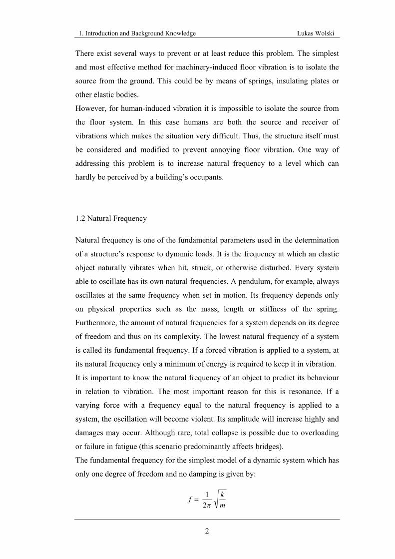
The fundamental frequency for the simplest model of a dynamic system which has
only one degree of freedom and no damping is given by:
mkf
21 π
=
1. Introduction and Background Knowledge Lukas Wolski
3
In this case the natural frequency simply depends on the stiffness k and the total
mass m of the system. This equation indicates the importance of these two
qualities for a dynamic system. For concrete floors, the stiffness is composed of
further three factors: it depends on Young's modulus, Poisson’s ratio and the
moment of inertia of the considered structure.
To minimise the perception of floor vibration it is important to achieve as high as
possible values for the system’s natural frequencies. This will occur if the
stiffness is very high and the mass is by contrast very low. This is the ideal case
which will result in very high frequencies. The opposite effect happens if a high
mass in combination with a low stiffness starts to vibrate and therefore this
situation should be avoided.
1.3 Cobiax flat slab
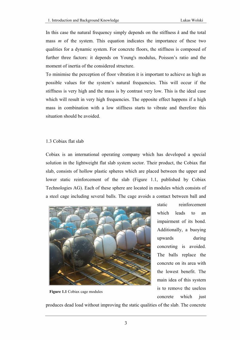
Cobiax is an international operating company which has developed a special
solution in the lightweight flat slab system sector. Their product, the Cobiax flat
slab, consists of hollow plastic spheres which are placed between the upper and
lower static reinforcement of the slab (Figure 1.1, published by Cobiax
Technologies AG). Each of these sphere are located in modules which consists of
a steel cage including several balls. The cage avoids a contact between ball and
static reinforcement
which leads to an
impairment of its bond.
Additionally, a buoying
upwards during
concreting is avoided.
The balls replace the
concrete on its area with
the lowest benefit. The
main idea of this system
is to remove the useless
concrete which just
produces dead load without improving the static qualities of the slab. The concrete
Figure 1.1 Cobiax cage modules
1. Introduction and Background Knowledge Lukas Wolski
4
forms a hard shell with struts by using appropriately located cavities formed by
hollow spheres. Nevertheless the slab has the same load bearing behaviour as
traditional solid slabs and brings along some improvements to them. First of all
Cobiax slabs weighs up to 35% less than solid slabs of equivalent dimensions.
This has a positive effect on the number of necessary vertical bearing elements
(up to 40% less column usage). It is also feasible to create large spans, up to more
than 20 m, without using beams. These two factors increase the possibilities of
open areas in buildings, making more alterations possible. Furthermore, the mass
reduction is noticeable in designing foundations, leading to savings in the amount
of material used. Other advantages include reductions in CO2 emissions, savings
in the amount of reinforcement needed, the application of all common standard
designs and the smooth bottom view. This, the common formwork and the biaxial
load bearing made possible by the hollow section’s spherical shape are also
advantages over common hollow concrete slabs such as waffle decks.
During the design process a few changes concerning the slab’s specific qualities
should be considered, including the decrease in stiffness for Cobiax slabs caused
by the reduced moment of inertia compared to a solid slab. For this purpose
numeric factors have already been determined and can be easily used for
conversion (see Appendix C). Besides small modifications the whole design
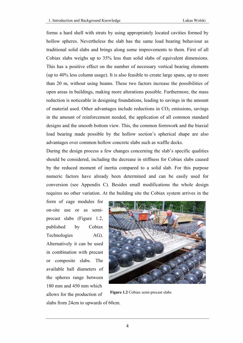
requires no other variation. At the building site the Cobiax system arrives in the
form of cage modules for
on-site use or as semi-
precast slabs (Figure 1.2,
published by Cobiax
Technologies AG).
Alternatively it can be used
in combination with precast
or composite slabs. The
available ball diameters of
the spheres range between
180 mm and 450 mm which
allows for the production of
slabs from 24cm to upwards of 60cm.
Figure 1.2 Cobiax semi-precast slabs
1. Introduction and Background Knowledge Lukas Wolski
5
1.4 Aims and Objectives
The general aim of this dissertation is to investigate the impact of Cobiax flat
slabs’ specific qualities on their fundamental frequencies in comparison to solid
concrete floors. As in both main numerical factors for the fundamental frequency
the stiffness as well as the mass of the subject is decreased, the consequence for
the slabs’ behaviour in case of natural frequency should be researched. The result
should clarify if and how these different qualities affect the slabs’ performance.
Furthermore it should deliver an overview of the treatment of concrete floors’
natural frequencies in structural engineering.
This study investigates three objectives. Firstly, due to varying estimations
concerning the limits of structures’ natural frequencies, different evaluations
following national codes and independent recommendations will be presented.
Afterwards a compilation of simplified methods for hand calculations will be
provided. They will be tested in some example calculations and their accuracy
when compared with “finite element values” will be investigated. The third
objective is the main area of this research. A precise comparison of Cobiax flat
slabs and traditional solid slabs will be undertaken using finite element software.
The data yielded will then be thoroughly analysed. This will result in a detailed
evaluation of the characteristic qualities of a Cobiax flat slab.
1. Introduction and Background Knowledge Lukas Wolski
6
1.5 Purpose of Research
This research is developed in collaboration with Cobiax Technologies GmbH,
Darmstadt, Germany and Cobiax Technologies Ltd, London. To market their
product effectively Cobiax must possess all necessary information concerning its
structural behaviour. Some areas of performance are yet to be investigated,
including the Cobiax slabs’ behaviour in relation to natural frequency; a detailed
comparison with a conventional concrete solid slab is also required. As already
explained, natural frequency in this context depends on two major factors. The
first is the stiffness of a slab which depends on its basic material as well as
geometry. Compared to a solid slab the material property is the same but due to its
hollow inside section, the Cobiax flat slab has a different geometry. This results in
a lower stiffness, which indicates a decrease in its natural frequency.
The second key component of the equation for natural frequency is the mass.
Contrary to the stiffness, where the hollow sections of the spheres have a negative
influence, in the case of mass they are an advantage. The one-third reduction in
concrete becomes perceivable and increases the value of natural frequency. The
decrease of both values has an opposite effect; one will improve the solution and
the other will impair it. The question is how much these characteristics impact on
the product’s performance and so which is to be the decisive factor in the final
evaluation and recommendations.
The research will carry out a clear investigation of this problem and deliver an
unambiguous judgement. It is important to explore all possible advantages of the
Cobiax flat slab as, in the future, this research may help to convince clients
worried about the effects of the slabs’ lower stiffness on its dynamic qualities.
1. Introduction and Background Knowledge Lukas Wolski
7
1.6 Literature review
1.6.1 Human Response to Floor Vibration
Arthur Bolton (1994) explained the importance of dynamics in structural
engineering with the following sentence: “Crowds go to fairgrounds to be
subjected to quite large accelerations and enjoy the sensation, but if subjected to a
tiny fraction of that excitation in a building they might become sick or anxious.”
The psychological effect of vibrating structures, then, can be profound. It can
cause people discomfort, nausea or anxiety. Of course these are all extreme
reactions, but milder effects present a difficult problem because of wide variations
in human sensitivity. There is also dependence on whether subjects are alone or in
a group; one particularly sensitive person amongst other people can sometimes
trigger off a collective belief that a barely perceptible vibration is dangerous or
uncomfortable. Another criterion of percipience vibration is the activity which is
being pursued at the time. Usually people are more sensitive to vibration when
they are in a quiet and untroubled area rather than, for example, a busy region.
Furthermore the direction of vibrations affects the percipience. Investigations
show that a translation in a horizontal direction has more effect than one in a
vertical direction. As a result of all these factors it is difficult to set an accurate
borderline between ‘acceptable’ and ‘unacceptable’ levels of vibration. It is only
possible to provide data with ranges which are definitely unacceptable and thus
should be prevented.
Reiher and Meister (1931) performed investigations to obtain such ranges. People
of different ages, professions and provenances had to stand and lie on a vibrated
platform. The tests covered sinusoidal vertical as well as sinusoidal horizontal
vibration. The frequencies used started from 3 Hertz up to 70 Hertz and
amplitudes from 0.0001 to 1.0 cm, figures which approach realistic values. During
the tests, noise was an important factor. It was necessary to minimize noise as
much as possible so as not to disturb hearing and thus the results.
After a vibration impact of 5 minutes every subject had to evaluate their
“sentiences”. They had to organise their “sentiences” into six groups which
ranged from “not perceptible” to “very disturbing”. After finishing all tests, the
1. Introduction and Background Knowledge Lukas Wolski
8
results were plotted in charts showing frequency against amplitude. All results
were included in these charts and afterwards it was possible to draw borderlines
for each category. These charts are one possible means of evaluating the
consequences of vibration for the human body. In general Reiher and Meister
recommend avoiding the last two categories. Residential areas should also avoid
vibration from category 4 which translates as “keenly noticeable” vibration.
A similar investigation was carried out by Wiss and Parmelee (1974). They
extended the amount of subjected persons from 10 to 40 and confined the scope of
their tests to a standing position. All persons had to assess their perception using
five classifications. For a steady-state condition (0 damping) this investigation
showed a lower perceptible for a particular frequency and displacement compared
of those performed by Reiher and Meister. However, the performance and
analysis of the studies were not exactly the same and so could explain these
differences. Further results concerned the effect of changing the damping for the
perception of vibration. It was assumed that if the damping was increased from
0.02 to 0.20 of critical, the product of frequency and displacement would
approximately double.
In general Bachmann (1987) recommends avoiding frequencies below 7.5Hz for
office buildings made of reinforced concrete. This value ensures that even the
third harmonic is taken into consideration, which means, that besides to the
fundamental frequency its integer multiples are regarded. For example, if the
frequency is f, the harmonics have frequency 2f, 3f, 4f, etc. Compared to
pedestrian structures such as gymnasia or sport halls where it is sufficient to
regard the second harmonic, for office buildings it is necessary to consider the
third harmonic as the occupants are more sensitive. Not only the occupants,
however, should be protected against vibration. Human motions such as walking,
running, dancing and skipping are sufficient to cause overstressing of the
structure, and in extreme cases the loss of structural integrity, damage to non-
structural elements (e.g. claddings), and development of cracking or excessive
noise (e.g. due to reverberating equipment).
1. Introduction and Background Knowledge Lukas Wolski
9
Brownjohn (2001) investigated the energy dissipation from vibrating slabs due to
human-structure interaction. It was clarified how the presence of people located
on a vibrating structure affects its dynamic behaviour. For this purpose a simply
supported 7m x 1m x 0.075m prestressed concrete plank was forced to vibrate
while a subject was standing on it. Five different sets of test were performed,
including the subject sitting on a plastic chair, standing erect, with knees slightly
bent, with knees very bent and finally with a solid mass equivalent to the subject.
The results confirmed that the human body acts dynamically with the structure by
decreasing its natural frequency. This was explained by the fact that the effective
mass is increased as well, but it was also identified that the human body has a
beneficial effect concerning damping ratio because, depending on posture,
damping can increase significantly.
1.6.2 Case Studies
The importance of both vibration problems and proper fundamental frequencies is
shown by Hanagan (2005), who has published a paper containing several case
studies on walking-induced floor vibration in existing buildings. This type of
vibration is shown to affect different types of buildings including offices, a
classroom and a clothing store. In each of these cases, the cause of vibration was
people walking around the space.
In one case, occupants of an office building started to report annoying floor
vibration in 2004. Interestingly, this building was constructed in 1974 and there
had been no previous complaints concerning floor vibration. After an
investigation measuring the acceleration of the affected slabs, it was detected that
the fundamental frequency of this floor system was about 4.7 Hz. This value is not
acceptable nowadays but it shows that even low frequencies might work well in
special circumstances. After almost 30 years vibration problems occurred due to
the removing of partitions which resulted in reduced damping and a higher
vibration.
Another case study in this paper shows the importance of complying with current
recommendations for natural frequencies. In this study structural engineers
suggested a more substantial floor system, including a thicker slab, to meet
1. Introduction and Background Knowledge Lukas Wolski
10
recommendations designed to avoid vibration problems. However, as a result of
previous experience with this building type, the higher costs involved and the
absence of vibration problems in the past, the developer elected for a thinner
solution. Unfortunately he was wrong and the occupants perceived motions close
to walk paths. The complaints stopped immediately after additional support and
damping was created through the use of full-height partitions.
Further case studies were presented by Bachmann (1992). He published ten cases
of vibration problems produced by human activity. One example specified
serviceability problems in a two-story gymnasium. Every time the upper hall was
used by fitness classes, floor vibration was noticed in the hall below and glazed
exterior walls started to vibrate horizontally. Additional effects included rattling
of doors and shutters and clattering of equipment. An investigation was carried
out to determine the dynamical qualities of the floor. It was established that the
fundamental frequency was about 4.9 Hz. When people jumped with a frequency
of approximately 2.48 Hz, resonance was excited by the second harmonic. In
order to avoid annoying effects and possible fatigue damage the fundamental
frequency was improved to 7.3 Hz by increasing the floor’s stiffness.
Other cases discussed in this paper showed similar problems caused by low
fundamental frequency and excitation by humans which resulted in significant
modifications being made.
1.6.3 Consideration of Vibration in Design
Fisher and West (2001) divided the consideration of human response to floor
vibration into four major steps. First of all the natural frequency should be
calculated which is affected by acceleration due to gravity, Young’s modulus,
moment of inertia, supported weight and the span of the structure. Afterwards the
initial amplitude should be calculated. Damping of a floor is another essential
factor as it affects the duration and nature of the vibration: physical tests showed
damping percentages ranging from 3% for bare floors to 6% for finished floors
and up to 13% for finished floors with partitions. The fourth factor is a standard of
measure involving the previous three figures. For this purpose graphs are used,
1. Introduction and Background Knowledge Lukas Wolski
11
with axes showing the frequency and displacement amplitude. The human
response to these factors is then plotted.
The adverse effects and therefore the necessary avoidance of resonance were
illustrated in a report by Cooney and King (1988). It was claimed that, due to
resonance, the motion of a floor may be magnified by up to 20 times its static load
condition. A significant increase in acceleration, velocity and displacement
occurs; an effect which should be avoided by all means. For this purpose the
authors provided a design method to identify a possible risk of resonance for
floors: specifically, vibration induced by human activities. First the expected load
of the area including all participants and their activities had to be assessed.
Occupants’ activities will lead to an appropriate forcing frequency and their total
load in combination with a particular factor will give the dynamic load. Special
literature, for example the BS 6472 (1992), will provide values for the acceptable
limiting of acceleration. The final steps are the determination of the total floor
load including the dynamical load component and further the calculation of the
fundamental frequency for the structure. With the help of these data and a special
equation presented by the authors an initial check of potential resonance may be
made. Where the acceptable level of acceleration was exceeded, increasing the
stiffness was suggested along with relocating or controlling the activity or just
accepting the discomfort.
The Canadian Institute for Scientific and Technical Information (1980) published
a paper to provide a better understanding of vibration due to dynamical loads. The
paper was specified to human induced vibration and gave a general overview of
this topic. The maximum walking frequency for a person was given as 3 Hz; the
approximate frequency for jumping was 5 Hz, but as also told, these values were
unlikely to be reached. Also included were approximated equations for the
fundamental frequency of simply supported, clamped and cantilever beams and
uniaxial plates. Furthermore the relationships between static and dynamic
deformation and vibration behaviour under periodic and single loads were shown
by equations and examples. The example given of a group jumping in a
gymnasium clarified that static deflection remains unchanged for different
1. Introduction and Background Knowledge Lukas Wolski
12
fundamental frequencies. However, the dynamical deflection increased for a
reduced frequency and reached extreme values in the case of resonance.
Crist and Shaver (1976) complained about insufficient investigation of floor
vibration in national codes. The accuracy of an evaluation for floor vibration can
be complicated by such factors as a lack of necessary components. In addition the
structure location, the type of structure, the type of occupancy and damping
should be considered in literature. An additional cause for concern was the
insufficient provision of data for evaluation which must then be qualified through
further research.
Furthermore, this publication explained the complexity surrounding the
determination of human activity and occupant response. Both are random
variables. The dynamic load caused by the former depends on varying
characteristic factors including walking gait, variation in weight, heel-to-ball of
foot contact and footwear. Influences on the perception go beyond the technical
values of frequency, direction and duration to encompass psychological factors in
form of mental state, motivation and experience and the physical factors of sound
and sight.
1.6.4 Two Way Hollow Decks
An overview of the general structural performance of biaxial hollow section slabs
of the type Cobiax produces is presented by Pfeffer (2002), who investigated the
slabs’ bond between reinforcement and concrete, flexure load-bearing capacity,
deflection and punching behaviour. Initial tests showed that due to the contact of
spheres with reinforcement the bond between reinforcement and concrete
decreased in these areas. This led to a development of reduction factors and
furthermore to a suggestion for improving slab design by relocating the spheres
from the reinforcement. However, the flexure load-bearing capacity of a two-axis
hollow slab is comparable to a solid slab. If the concrete compression zone is
above the sphere, it can be dimensioned as a rectangular cross-section by means
of the usual methods. As a result of the decreased self-weight the bending
performance of a hollow section slab is better than a solid slab. This occurs up to
1. Introduction and Background Knowledge Lukas Wolski
13
an external load-to-self weight ratio of 1:5. In case of punching it was discovered
that load capacity is approximately 50% lower if spheres are included. To avoid
this disadvantage, it is recommended that spheres are removed from inside the
punching area. This results in a similar punching capacity to solid slabs and
allows for a common punching design.
Another structural behaviour, the transverse force capacity, was investigated by
Schnellenbach-Held (2003). A comparison between biaxial hollow section slabs
and conventional concrete solid slabs showed the differences in their shear force
performance. Though the load-bearing capacity before and after shear crack
formation was similar, the failure load of the lightweight slabs was about 45%
lower than the breaking load achieved with solid slabs. This can be explained by
the reduced concrete area which decreases the transmission of tensile stresses. For
slabs without shear reinforcement, this is the main impact on transverse force
capacity.
1.6.5 Comparison of FEM and Field Tests
The results discussed in this research can be compared to the real behaviour of
Cobiax slabs. Emad El-Dardiry et al. (2002) ran an investigation which yielded
good results. He and his colleagues compared measured natural frequencies of an
existing building with values calculated by different finite element models. For
this purpose and as a part of the European Concrete Building Project (ECBP) a
realistic office building was constructed inside the BRE Cardington Laboratory. It
was a seven-storey in-situ concrete building consisting of long-span flat slabs
supported by columns designed to Eurocode 2. Each floor was 3.75m high, giving
a total height of 26.25 m. The building had three bays of 7.50 m constituting a
width of 22.50 m and four bays of 7.50 m making a length of 30.00 m. All slabs
were designed as reinforced concrete flat slabs with 0.25m thickness. The
intended imposed load was 2.5 kN/m².
After finishing the construction, Building Research Establishment Ltd conducted
dynamic tests on the floors. The tests involved monitoring the acceleration of the
centre of each floor area in response to a heel-drop. The response was then
1. Introduction and Background Knowledge Lukas Wolski
14
converted to an autospectrum using a “Fast Fourier Transform” procedure and the
dominant natural frequency was identified. All seven floors were covered by
measurements from 11 different locations on each floor. The measurements
provided a basis for evaluating the quality of different FE models. Consequently,
FE analysis of several commonly used models was conducted, and the numerical
and experimental results compared. The engineers used the FE software LUSAS
and modelled different approaches to floor-column connection.
One result of this investigation was that, while the different models used in this
study give different frequencies, the mode shapes are similar in a global sense. All
approaches had a variance of between 2% and 17% from the measured values.
The average difference was 12%. Another conclusion of a prior investigation was
the negligible effect of mesh size on dynamic behaviour. In case of natural
frequency all three meshes considered had no significant impact. However, they
affected the appearance of the mode shapes and so a fine mesh was used.
A similar comparison was performed by Williams et al. (1993). Tests were carried
out on reinforced and prestressed concrete floors of various configurations,
covering the full range of spans and thicknesses encountered in typical structures.
Newly cast, bare floors as well as already finished floors including false floors
and services were tested. The building types tested included offices and car parks.
These types are structurally quite similar with the exception of the lack of any
finishes on the floor of the car park, which results in lower damping values.
The experimental set-up used a hammer test, in which a soft-tipped hammer
generates the input excitation through a striking motion. By using other
experimental equipment general vibration qualities such as natural frequencies,
mode shapes or damping ration were determined. A single bay within the test
floor was chosen as the test panel and divided into a 5 x 5 grid of equally spaced
points. Afterwards every point was investigated five times to obtain an averaged
response for each specific point. Later a finite element model was created using I-
DEAS finite element software to compare the gained values.
A detailed comparison was given here for the specific example of a car park in
Wycombe. The car park consisted of a 0.21m thick slab, supported by post-
tensioned beams along column lines.
1. Introduction and Background Knowledge Lukas Wolski
15
The results of this comparison show that the computer model gives very good
estimates for the first three frequencies. All three frequencies are quite similar to
those investigated. The averaged difference between both results is about 4%.
It was supposed that, due to the increasing importance of accurately representing
the boundary condition, natural frequencies of higher modes would exhibit less
similarity. However, as when assessing potential human discomfort due to
vibration only the first few frequencies are important, the investigation concluded
that it is possible to obtain a reasonable estimate of the dynamic characteristics of
a floor by using finite element software.
Osborne and Ellis (1990) have presented a study of vibration design and testing of
long-span lightweight floors, focussing on the estimation and evaluation of floor
design. One major objective was the comparison between simplified hand
calculations, computer supported calculations and accurate tests on-site. It was
shown that all three, and especially the latter cases, predict similar values; the
estimated frequency of a computer analysis was just 0.16 Hz (approximate 3%)
higher than measured frequency.
Another interesting finding of this study was the change in dynamic behaviour
from the bare floor to a finished floor including a false floor, service installations
and fire protection. Although the finished floor showed only a small increase of
damping and stiffness, qualitative observation by people performing a heel drop
test agreed an improved perception.
The vibration assessment floor from Ove Arup & Partners (2004) provides
particularly useful information because of its strong resemblance to the Cobiax
flat slab system. The report includes the results of an investigation into the
vibration behaviour of a floor for a typical hospital. For this case an idealised area
of hospital floor was assumed. Its properties included 400mm thickness, 315mm
ball size and 3 x 3 square bays. Each bay had a span of 9m x 9m. The imposed
loads were estimated as realistic in-service values averaged over the entire floor
area. Using the finite element software MSC NASTRAN, a model was created to
analyse the floor’s dynamic performance. The slab was modelled as a 400mm
thick solid slab and its specific qualities were considered by a reduced stiffness
1. Introduction and Background Knowledge Lukas Wolski
16
and mass. The analysis showed that the fundamental frequency of this floor is
11.8Hz. Furthermore a footfall response analysis was carried out to obtain the
root-mean-square (r.m.s.) velocity of the floor. Afterwards all results were
compared with a floor of 400mm solid concrete. The first natural frequency
reduces to 10.4Hz, a decrease of 12%. The responses for Bubbledeck slabs are
16% higher than those for a solid slab of the same 400mm thickness.
1.6.6 Determination of Frequency
Mazumdar (1971) determined the fundamental frequency of elastic plates of
arbitrary shape by aid of constant deflection lines. For this purpose he assumed
the classical small-deflection theory to be valid. His method for the case of
elliptical plates was illustrated specifically because of its increased complexity
compared to other shapes. The assumption that the lines of equal deflection also
had an elliptical shape was made in response to the problem of determining the
resulting time-dependent deflection field. This approximation is then only valid
for slender elliptical plates, making this method only practical for thin plates.
After the determination of all necessary dynamical equations, two examples were
calculated. One plate was supposed to have clamped edges and the second was
simply supported, an estimation which had previously only been published in one
work. Furthermore the author compared his method with results already
established in literature. For small ratios of both semi-lengths this comparison
showed very similar outcomes to the other present values.
Jones (1975) used this method and extended the comparison. He investigated
simplified calculations for the fundamental frequency of structures with different
shapes and boundary conditions such as equilateral triangular, rectangular or
semicircular plates. Afterwards he also compared these approximations with
computed and more exact values. As before, the results of this comparison were
very good. For the example of a clamped quadratic plate, the difference between
the two estimations was 0.05%.
1. Introduction and Background Knowledge Lukas Wolski
17
Magrab (1976) adopted a different approach to estimating the natural frequencies
for plates. He derived an expression for orthotropic rectangular plates with simply
supported, elastically supported or clamped boundary conditions. Instead of using
existing estimation methods and thin-plate theory which relies on a length-to-
thickness ratio he solved the problem with another mathematical technique: the
Mindlin-Timoshenko theory. This theory is an improvement on the Euler-
Bernoulli beam theory, which condensed a beam to a 1-D structure. Another
assumption of this theory is that the plane cross-section of a beam remains plane
and normal to the reference line when the beam deforms due to bending.
In addition to this hypothesis Timoshenko's theory considers sheer and rotational
inertia effects and the resulting deformation. Comparing an example with other
estimations which use the thin-plate theory yielded analogical values with
differences between 0.08% and 3.7%. Excepting the estimate values of Elishakoff
(1974), all other fundamental frequencies are higher than those calculated by the
author. This results from the consideration of transverse sheer and rotary inertia
which also imbibes vibration energy additional to bending as required by the thin-
plate theory.
The influence of Timoshenko’s additional consideration, rotational inertia and
sheer deformation for rectangular plates, was formerly investigated by Mindlin,
Schacknow and Deresiewicz (1956) who determined a method to obtain natural
frequencies with coupled modes. Special regard was given for the case of a plate
with one pair of parallel free edges and the other pair simply supported.
Leissa (1973) presented a study of approximate formulas for free vibration of
rectangular plates. It was the first compilation of all 21 cases which involved all
possible combination of classical boundary conditions, like clamped, simply
supported and free edges. Amongst other techniques he used the Ritz method or
the beam function for this purpose. This led to the production of a set of 21 tables
for the estimation of the first 9 modes for each plate including different length-to-
width ratios. Furthermore the effect of changing Poisson’s ratio on the natural
frequencies was presented. In every case the frequency depends on Poisson’s
ratio. An example of a plate supported on two parallel edges by simply-supports
2. Human Response and Acceptance Criteria Lukas Wolski
18
and on the other a pair of free edges showed that increasing Poisson’s ratio caused
a decrease in natural frequency. Other objectives of this investigation were the
evaluation of accuracy compared to the referenced Warburton’s formulas for
natural frequencies and the effect of changing edge condition upon the frequencies
and their accuracy.
2. Human Response and Acceptance Criteria
Evaluation of measured or calculated values of floor vibration must be carried out
in order to predict its influence on the surrounding environment. This requirement
creates the need for specific acceptance criteria. It is possible to classify the
effects floor vibration has on its environment into three main areas:
- Overstressing of structural members
- Physiological effect on people
- Impact of production processes with sensitive equipment or susceptible
machinery in general
(Bachmann and Ammann, 1987)
Of these three, most attention is paid to human response. This is because damage
and fatigue failure of structural elements due to walking-induced floor vibration
are unusual, and every different type of machinery has its own very specific
requirements. Different acceptance criteria and recommendations have been
developed to measure human response. Unfortunately, though, it is not possible to
provide exact limit values and this can obviate perception of motion. As the
variety of human responses to floor vibration varies greatly, these criteria can only
utilise reference values gained by experience or field tests. The complexity of both
perception levels and human sensitivity to vibration is illustrated by a high
number of interrelated factors. Among them are:
Direction of motion: Humans evaluate every direction of motion
differently. Generally vertical foot-to-head vibration
is considered more annoying than horizontal chest-
2. Human Response and Acceptance Criteria Lukas Wolski
19
to-back vibration (Cooney and King 1988).
However, every direction of motion has to be
considered because of its potential occurrence.
While horizontal vibration causes only small
concern in offices and other workplaces, its
importance increases in the design of residences and
hotels where sleeping comfort must be considered.
Personal characteristics: Different responses are given depending on the age,
sex and level of concentration of the subjects as well
as those of surrounding community.
Timing and duration: Motions at night are less tolerated than those
occurring during the day. Furthermore continuous
motion (steady-state) is more annoying than motion
caused by infrequent impact (transient).
Expectation: If subjects are forewarned of vibration, their
perception will be less sensitive
Current activity: Different levels of acceptance exist for office work,
physical work, resting, dining and dancing.
Acceptance levels are also affected by the
surrounding environment (e.g. home, office or
gymnasium).
Since the pioneering work of Reiher and Meister (1931), most vibration criteria
provide graphs defining regions of acceptable and unacceptable vibration. Usually
these are plotted in frequency versus peak acceleration due to gravity of the floor
vibration, but other numerous parameters such as velocity or displacement of the
treated floor can be included. On the graph, single lines represent a constant level
of human reaction (isoperceptibility lines) with the region above a line denoting
unacceptable vibration. These act as boundaries between different levels of
perception.
2. Human Response and Acceptance Criteria Lukas Wolski
20
2.1 Recommendations in Codes
2.1.1 British Standard
In British Standard BS6399-1:1996 Annex A, two different approaches are
recommended for the design of domestic and residential structures, especially
single family buildings. In areas subjected to dancing or jumping there can be an
increased risk of unpleasant floor movement and even resonance may occur. In
order to avoid this phenomenon, it is recommended that vertical natural frequency
is limited to at least to 8.4Hz and horizontal natural frequency to a minimum of
4.0 Hz. These frequencies should be calculated for the empty structure.
Another approach is to consider dynamic loads as well as dead and static imposed
loadings during the design stage. Deformation due to dynamic loads should not
exceed limits appropriate to the building or structure type.
No detailed specifications are provided for lightweight and long span structures.
Only the general advice of taking floor vibration into account and the
recommendation of specialist guidance documents are given:
Where lightweight and long span structures are used as concourses and public spaces,
they are likely to be subjected to inadvertent or deliberate synchronized movement by
people, causing dynamic excitation. The design provisions should take account of the
nature and intended use of the structure, the potential number of people and their possible
behaviour. Structural design should be undertaken with the help of specialist advice and
specialist guidance documents, as required by the appropriate certifying authority.
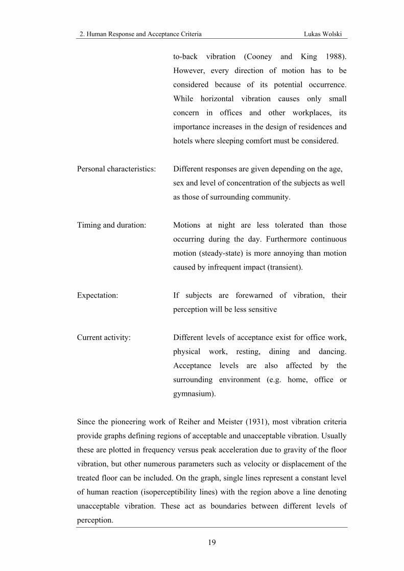
A more detailed treatment of floor vibration is covered by the British Standard
BS 6472:1992 “Guide to evaluation of human exposure to vibration in buildings
(1 Hz to 80 Hz)”. This guide has a general approach, for application to many
vibratory environments. It is applicable to vibrations transmitted through the
supporting surface to the body as a whole by considering different positions and
all three axes, as defined in figure 2.1.
Within the range of 1 to 80 Hz, the guide also considers different types of
structures including offices, residential buildings or critical working areas such
2. Human Response and Acceptance Criteria Lukas Wolski
21
x-axis: back to chest
y-axis: right side to left side
z-axis: foot to head
as operating theatres. All allowable vibrations are provided in curves of
annoyance for humans in terms of direction of transmission, frequency and
acceleration or velocity. While acceleration is given as r.m.s. acceleration (root-
mean-square acceleration), velocity is specified as a peak value. In terms of
human response the British Standard divides vibrations into two classes:
impulsive and continuous vibration.
Impulsive vibration is defined as a rapid build-up to and decrease from a peak; for
example vibration caused by the impact of a single heavy object on a floor. This
type may also consist of several cycles of vibration providing that duration is
short (less than approximately 2 seconds). The other category describes
continuous vibration which remains uninterrupted over a certain time period (for
example vibration caused by a group of people walking). Their different
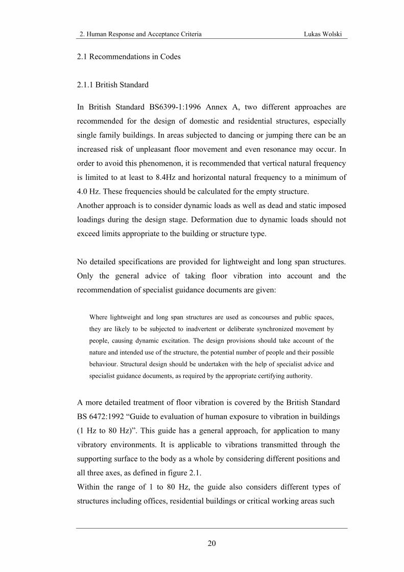
consideration is given by individual multiplication factors shown in table 2.1.
These factors are used to multiply the base curves and obtain the according curve
for a specific case.
Figure 2.1 BS 6472 (1992) Coordinate systems for vibration influencing humans
2. Human Response and Acceptance Criteria Lukas Wolski
22
Multiplying factors (see notes 1 and 5)
Place Time Exposure to continuous
vibration [16 h day, 8 h night] (see note 2 and Appendix B)
Impulsive vibration excitation with up to 3 occurrences
(see note 8)
Day 1 1 Critical working areas (e.g. hospital operating theatres, precision laboratories (see notes 3 and 10)
Night 1 1
Day 2 to 4 (see note 4) 60 to 90 (see notes 4 and 9, and Appendix B)
Residential
Night 1.4 20
Day 4 128 (see note 6) Office Day
Night 4 128
Day 8 (see note 7) 128 (see notes 6 and 7) Workshops
Night 8 128
NOTE 1 Table 5 leads to magnitudes of vibration below which the probability of adverse comments is low (any acoustical noise caused by structural vibration is not considered).
NOTE 2 Doubling of the suggested vibration magnitudes may result in adverse comment and this may increase significantly if the magnitudes are quadrupled (where available, dose/response curves may be consulted).
NOTE 3 Magnitudes of vibration in hospital operating theatres and critical working places pertain to periods of time when operations are in progress or critical work is being performed. At other times magnitudes as high as those for residences are satisfactory provided there is due agreement and warning.
NOTE 4 Within residential areas people exhibit wide variations of vibration tolerance. Specific values are dependent upon social and cultural factors, psychological attitudes and expected degree of intrusion.
NOTE 5 Vibration is to be measured at the point of entry to the entry to the subject. Where this is not possible then it is essential that transfer functions be evaluated.
NOTE 6 The magnitudes for vibration in offices and workshop areas should not be increased without considering the possibility of significant disruption of working activity.
NOTE 7 Vibration acting on operators of certain processes such as drop forges or crushers, which vibrate working places, may be in a separate category from the workshop areas considered in Table 3. The vibration magnitudes specified in relevant standards would then apply to the operators of the exciting processes. NOTE 8 Appendix C contains guidance on assessment of human response to vibration induced by blasting.
NOTE 9 When short term works such as piling, demolition and construction give rise to impulsive vibrations it should be borne in mind that undue restriction on vibration levels can significantly prolong these operations and result in greater annoyance. In certain circumstances higher magnitudes can be used.
NOTE 10 In cases where sensitive equipment or delicate tasks impose more stringent criteria than human comfort, the corresponding more stringent values should be applied. Stipulation of such criteria is outside the scope of this standard.
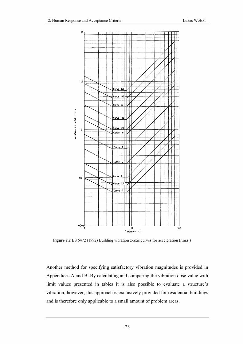
Figure 2.2 shows one example of a multiplied curve where the frequency is
plotted against the r.m.s. acceleration. It is recommended that the frequency-
acceleration combination is kept below the line which corresponds to the relevant
case, therefore minimising adverse comments or complaints of vibration.
Table 2.1 BS 6472 (1992) Multiplying factors
2. Human Response and Acceptance Criteria Lukas Wolski
23
Another method for specifying satisfactory vibration magnitudes is provided in
Appendices A and B. By calculating and comparing the vibration dose value with
limit values presented in tables it is also possible to evaluate a structure’s
vibration; however, this approach is exclusively provided for residential buildings
and is therefore only applicable to a small amount of problem areas.
Figure 2.2 BS 6472 (1992) Building vibration z-axis curves for acceleration (r.m.s.)
2. Human Response and Acceptance Criteria Lukas Wolski
24
2.1.2 German Standard
The German Institute for Standardisation published a similar code entitled DIN
4150-2 (1999) “Erschütterungen im Bauwesen; Einwirkungen auf den Menschen
in Gebäuden”. This code provides recommendations concerning humans’
vibration perception in residential and similarly used buildings and is applicable
to periodic as well as non-periodic vibrations. It also deals with frequencies from
1 to 80 Hz and considers all three axes of a human body as well as different types
of buildings; but in contrast to the English code, the German DIN uses a modified
parameter called KB value, which depends on the frequency of motion and was
established to assess the acceptance of motion by limiting the frequency to
specified values (see table 2.2).
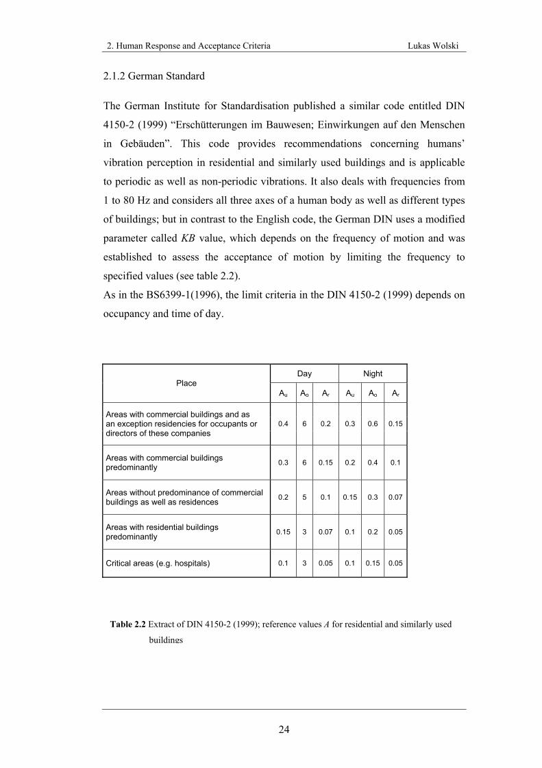
As in the BS6399-1(1996), the limit criteria in the DIN 4150-2 (1999) depends on
occupancy and time of day.
Day Night Place
Au Ao Ar Au Ao Ar
Areas with commercial buildings and as an exception residencies for occupants or directors of these companies
0.4 6 0.2 0.3 0.6 0.15
Areas with commercial buildings predominantly 0.3 6 0.15 0.2 0.4 0.1
Areas without predominance of commercial buildings as well as residences 0.2 5 0.1 0.15 0.3 0.07
Areas with residential buildings predominantly 0.15 3 0.07 0.1 0.2 0.05
Critical areas (e.g. hospitals) 0.1 3 0.05 0.1 0.15 0.05
Table 2.2 Extract of DIN 4150-2 (1999); reference values A for residential and similarly used
buildings
2. Human Response and Acceptance Criteria Lukas Wolski
25
For the comparison of measured and recommended limit values two different KB
parameters are used. These are represented by KBFmax for the maximum motion
and KBFTr , which is an averaged value spread over the assessment time. These
two values must be estimated for each of the three axes in which motion may
occur. The worst case becomes decisive.
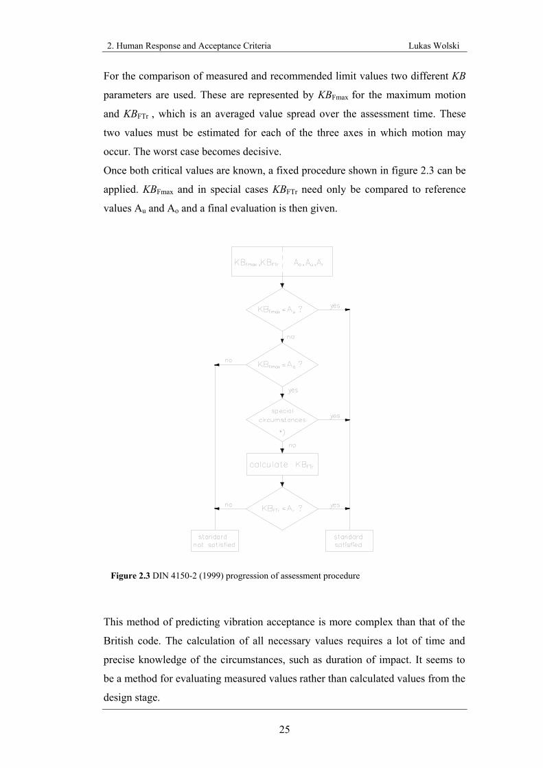
Once both critical values are known, a fixed procedure shown in figure 2.3 can be
applied. KBFmax and in special cases KBFTr need only be compared to reference
values Au and Ao and a final evaluation is then given.
This method of predicting vibration acceptance is more complex than that of the
British code. The calculation of all necessary values requires a lot of time and
precise knowledge of the circumstances, such as duration of impact. It seems to
be a method for evaluating measured values rather than calculated values from the
design stage.
Figure 2.3 DIN 4150-2 (1999) progression of assessment procedure
2. Human Response and Acceptance Criteria Lukas Wolski
26
2.2 Recommendations in Literature
Besides national codes and standards, many independent and individual
recommendations are available. These are partly developed from practical tests on
subjects and partly gained by experience of existing buildings. The following
paragraphs will deliver an overview of some of the recommendations found in
literature.
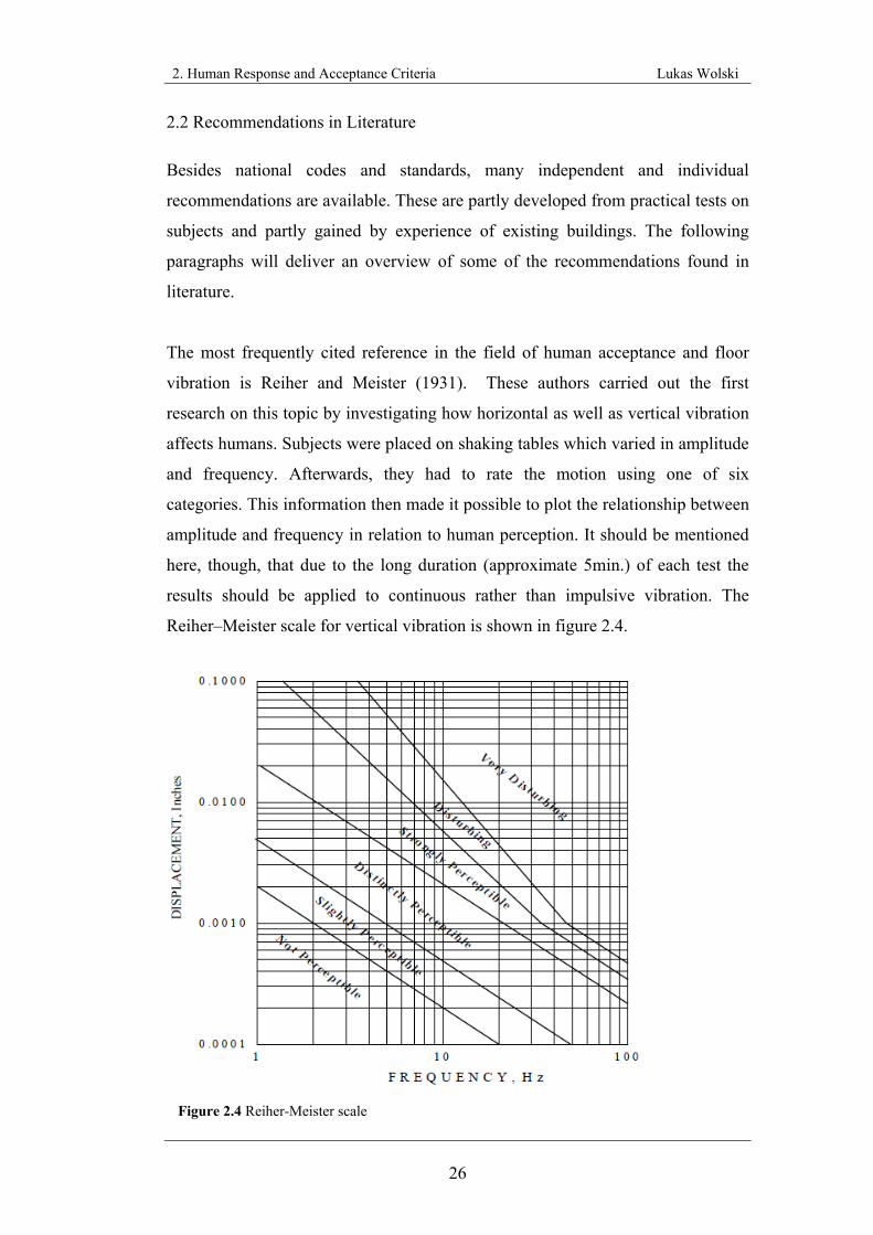
The most frequently cited reference in the field of human acceptance and floor
vibration is Reiher and Meister (1931). These authors carried out the first
research on this topic by investigating how horizontal as well as vertical vibration
affects humans. Subjects were placed on shaking tables which varied in amplitude
and frequency. Afterwards, they had to rate the motion using one of six
categories. This information then made it possible to plot the relationship between
amplitude and frequency in relation to human perception. It should be mentioned
here, though, that due to the long duration (approximate 5min.) of each test the
results should be applied to continuous rather than impulsive vibration. The
Reiher–Meister scale for vertical vibration is shown in figure 2.4.
Figure 2.4 Reiher-Meister scale
2. Human Response and Acceptance Criteria Lukas Wolski
27
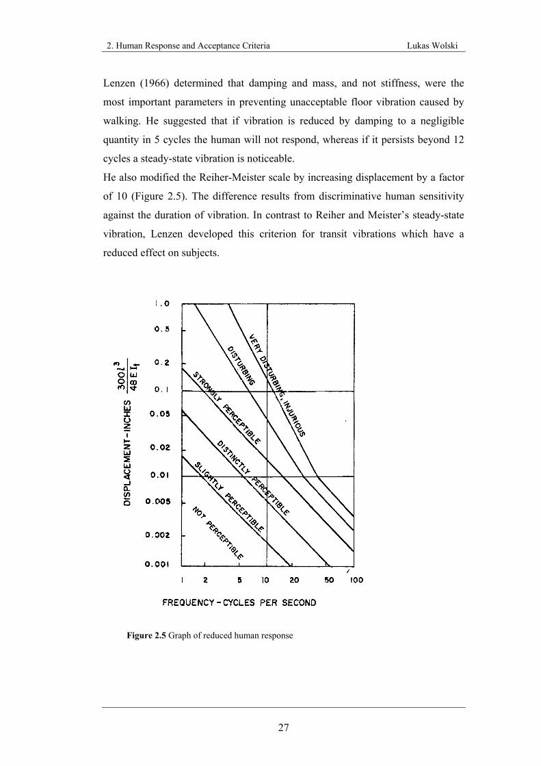
Lenzen (1966) determined that damping and mass, and not stiffness, were the
most important parameters in preventing unacceptable floor vibration caused by
walking. He suggested that if vibration is reduced by damping to a negligible
quantity in 5 cycles the human will not respond, whereas if it persists beyond 12
cycles a steady-state vibration is noticeable.
He also modified the Reiher-Meister scale by increasing displacement by a factor
of 10 (Figure 2.5). The difference results from discriminative human sensitivity
against the duration of vibration. In contrast to Reiher and Meister’s steady-state
vibration, Lenzen developed this criterion for transit vibrations which have a
reduced effect on subjects.
Figure 2.5 Graph of reduced human response
2. Human Response and Acceptance Criteria Lukas Wolski
28
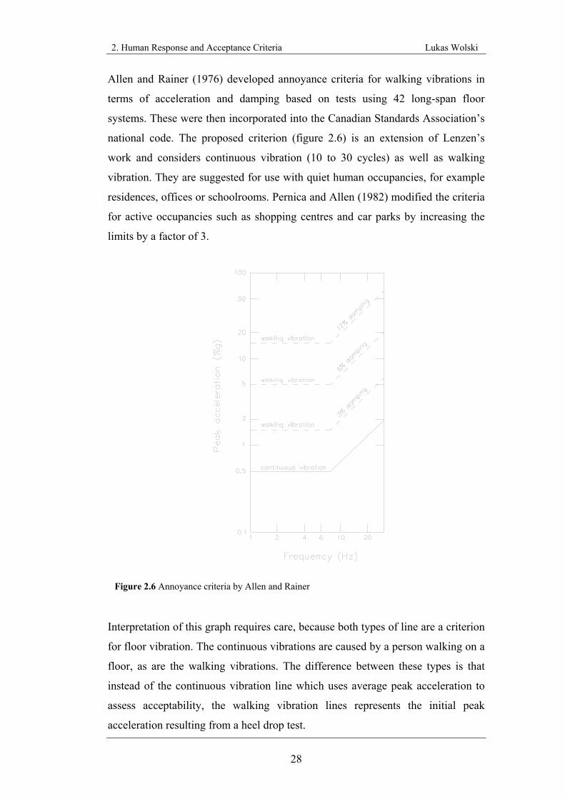
Allen and Rainer (1976) developed annoyance criteria for walking vibrations in
terms of acceleration and damping based on tests using 42 long-span floor
systems. These were then incorporated into the Canadian Standards Association’s
national code. The proposed criterion (figure 2.6) is an extension of Lenzen’s
work and considers continuous vibration (10 to 30 cycles) as well as walking
vibration. They are suggested for use with quiet human occupancies, for example
residences, offices or schoolrooms. Pernica and Allen (1982) modified the criteria
for active occupancies such as shopping centres and car parks by increasing the
limits by a factor of 3.
Interpretation of this graph requires care, because both types of line are a criterion
for floor vibration. The continuous vibrations are caused by a person walking on a
floor, as are the walking vibrations. The difference between these types is that
instead of the continuous vibration line which uses average peak acceleration to
assess acceptability, the walking vibration lines represents the initial peak
acceleration resulting from a heel drop test.
Figure 2.6 Annoyance criteria by Allen and Rainer
2. Human Response and Acceptance Criteria Lukas Wolski
29
Allen and Murray (1993) mentioned the necessity of the first three harmonics in
avoiding resonance. The third harmonic should be considered for a single person
walking with normal velocity. For jogging or more than one person, only the first
two harmonics are important. If the number of persons walking on a structure
increases then the dynamic loading does increase, but at the same time lack of
coherence at higher harmonics increases. However, generally such cases are rare
enough to not be a problem in practice.
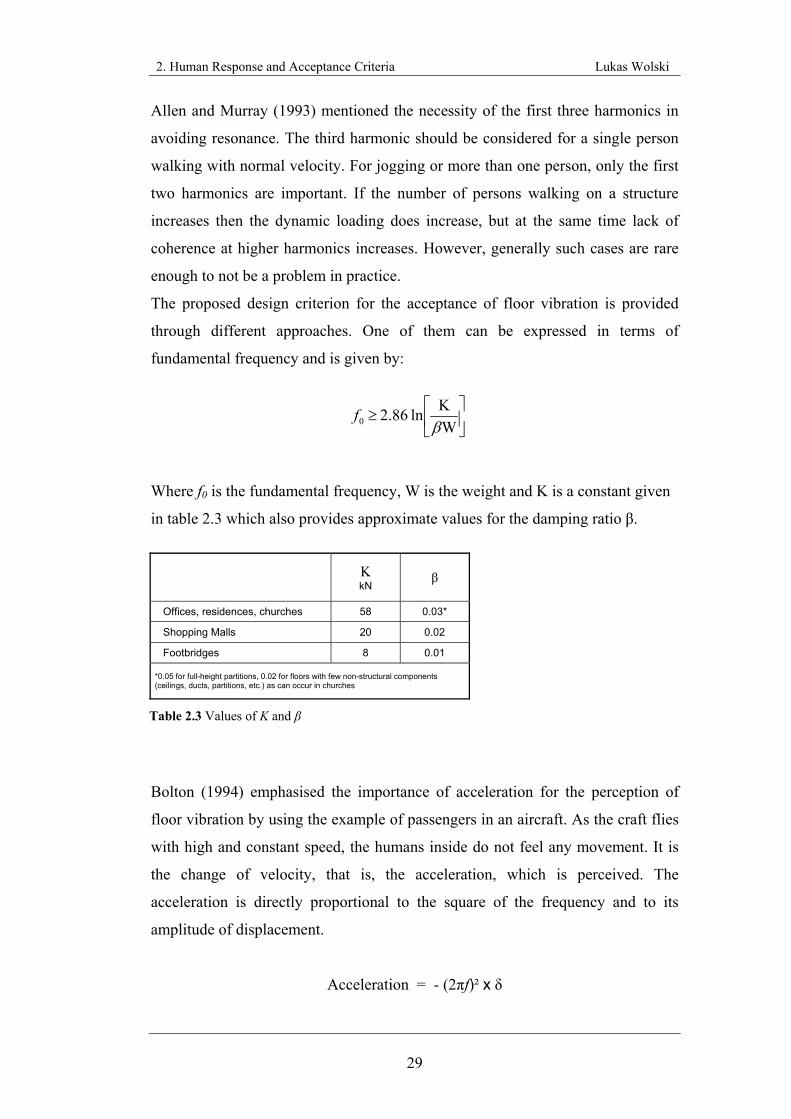
The proposed design criterion for the acceptance of floor vibration is provided
through different approaches. One of them can be expressed in terms of
fundamental frequency and is given by:
⎥⎦
⎤⎢⎣
⎡≥
WKln 2.86 0 β
f
Where f0 is the fundamental frequency, W is the weight and K is a constant given
in table 2.3 which also provides approximate values for the damping ratio β.
K kN β
Offices, residences, churches 58 0.03*
Shopping Malls 20 0.02
Footbridges 8 0.01
*0.05 for full-height partitions, 0.02 for floors with few non-structural components (ceilings, ducts, partitions, etc.) as can occur in churches
Bolton (1994) emphasised the importance of acceleration for the perception of
floor vibration by using the example of passengers in an aircraft. As the craft flies
with high and constant speed, the humans inside do not feel any movement. It is
the change of velocity, that is, the acceleration, which is perceived. The
acceleration is directly proportional to the square of the frequency and to its
amplitude of displacement.
Acceleration = - (2πf)² x δ
Table 2.3 Values of K and β
2. Human Response and Acceptance Criteria Lukas Wolski
30
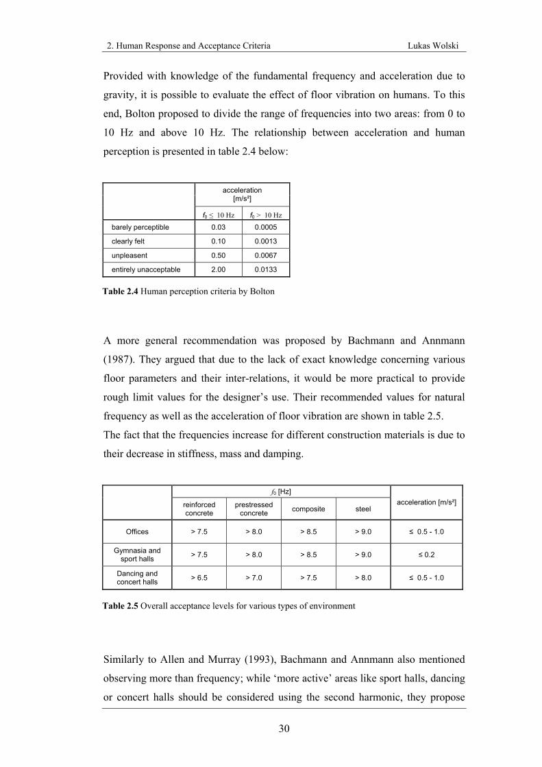
Provided with knowledge of the fundamental frequency and acceleration due to
gravity, it is possible to evaluate the effect of floor vibration on humans. To this
end, Bolton proposed to divide the range of frequencies into two areas: from 0 to
10 Hz and above 10 Hz. The relationship between acceleration and human
perception is presented in table 2.4 below:
acceleration [m/s²]
f0 ≤ 10 Hz f0 > 10 Hz
barely perceptible 0.03 0.0005
clearly felt 0.10 0.0013
unpleasent 0.50 0.0067
entirely unacceptable 2.00 0.0133
A more general recommendation was proposed by Bachmann and Annmann
(1987). They argued that due to the lack of exact knowledge concerning various
floor parameters and their inter-relations, it would be more practical to provide
rough limit values for the designer’s use. Their recommended values for natural
frequency as well as the acceleration of floor vibration are shown in table 2.5.
The fact that the frequencies increase for different construction materials is due to
their decrease in stiffness, mass and damping.
f0 [Hz]
reinforced concrete
prestressed concrete composite steel
acceleration [m/s²]
Offices > 7.5 > 8.0 > 8.5 > 9.0 ≤ 0.5 - 1.0
Gymnasia and sport halls > 7.5 > 8.0 > 8.5 > 9.0 ≤ 0.2
Dancing and concert halls > 6.5 > 7.0 > 7.5 > 8.0 ≤ 0.5 - 1.0
Similarly to Allen and Murray (1993), Bachmann and Annmann also mentioned
observing more than frequency; while ‘more active’ areas like sport halls, dancing
or concert halls should be considered using the second harmonic, they propose
Table 2.4 Human perception criteria by Bolton
Table 2.5 Overall acceptance levels for various types of environment
2. Human Response and Acceptance Criteria Lukas Wolski
31
high tuning with respect to the third harmonic of load-time function for offices or
other quiet working places.
Other literature presents this topic with less accuracy and provides only rough
limit values for consideration during the design of floor systems.
For the prevention of resonance Fisher and West (2001) recommend avoiding
natural frequencies of between 1 and 4 Hz for ‘walking areas’ and 5 Hz for
‘dancing areas’.
Cooney and King (1988) mentioned that crowds involved in activities such as
dancing or gymnastic can be synchronised by music or other means up to
frequencies of 6 Hz. Beyond this limit they become uncoordinated and a random
forcing function results. Therefore they suggest checking floors with natural
frequency below 6 Hz and possible support of assembly occupancies for
resonance.
Furthermore, Hanes (1970) reported that studies using automobile and aircraft
passengers showed that the natural frequency of human internal organs is between
5-8 Hz. Therefore, floor systems with natural frequencies in that range could
possibly cause human discomfort and should be avoided.
Morrison (2006) specified the interfering frequencies of individual sub systems
within the body. Some examples are the abdomen-thorax region, 3 Hz, the spine,
5 Hz or the heart, 7 Hz. The frequencies at which the whole human body is most
sensitive are 3 - 6 Hz and 10 - 14 Hz.
2.3 Summary
The effects of vibration on humans vary so widely that evaluation is very complex
and depends on many factors. In general, it is difficult to set accurate limits to any
parameters. However, past research has attempted to obtain boundaries for
different kinds of structures and activities. These should result in improved
ambience in new structures as well as decreasing the chance of justifiable
complaints made by users.
3. Simplified Hand-Calculation Methods Lukas Wolski
32
3. Simplified Hand-Calculation Methods
In the past, there have been many attempts to find simplified methods for
calculating the fundamental frequency of structures. Before finite element
software and computer packages, which predict all necessary information
accurately within a few seconds, this information needed to be estimated. Even
today, when computers are used universally, additional hand calculations are still
recommended because they help to give an initial assessment and are able to
forecast critical areas before or during the design stage. Alternatively, they might
be used as an additional check on results calculated by a computer (Weber 2002).
Simple equations and tables make it possible to estimate natural frequencies in a
very short space of time. Furthermore, only a few predictions are necessary, these
being material properties such as the Young's modulus or the Poisson ratio and
geometrical properties such as thickness of the structure or the length of span.
Equipped with this data and a simple calculator, fundamental frequency can be
predicted in seconds, provided the structure is not too complex. As the frequencies
of complex structures would require huge efforts to hand-calculate, methods are
only published for simple models such as one-span or continuous beams, one-span
slabs or chimneys and pylons. The simplification is usually based on beam theory
and can easily be adopted for these kinds of structures.
Another simplification of these methods is the assumption of boundary condition.
In reality, the grade of restraint for each support is unclear. Obviously in practice
the support conditions are rarely simply supported or truly fixed, but in
simplifications all supports are assumed to be 100% simply supported or clamped.
This produces only small inaccuracies compared with the real dynamic behaviour
of structures.
Other factors can also affect the accuracy between model and real behaviour.
There are some influences which a simplification cannot or will not predict. An
example of one such influence is the dissipation of energy due to contributions
from coating or a suspended ceiling. This increases the damping ratio and
therefore counteracts the vibration. Brownjohn (2001) also highlighted that a
certain amount of vibration is reduced by occupants standing on the floor, a factor
which cannot be predicted in hand calculations. Another difficulty is the non-
linearity which may occur after cracking. Once the concrete starts to crack, the
3. Simplified Hand-Calculation Methods Lukas Wolski
33
effective stiffness is in flux. Due to the smaller amount of concrete cross-section,
the moment of inertia decreases, resulting in a higher natural frequency.
These are a few circumstances which prevent 100% accurate values from being
made; nevertheless, in many cases simplified estimations can provide good
practical results and therefore initial ideas concerning the dynamical behaviour of
the structure. Thus, problematical areas can be identified in an early design stage.
This chapter deals with simplified methods for calculating the fundamental
frequency of slabs. For this purpose a summary of some existing literature
providing equations or tables is presented and is checked against their accuracy.
Therefore, calculations for a set of common structural slabs considering free
undamped natural frequency for rectangular isotropic plates are carried out
(Appendix A). Afterwards each example is compared against more exact values
calculated by finite element software, enabling a general evaluation of their
practical use to be undertaken.
3.1 Common Mathematic Techniques
When estimating the necessary values of eigenvalues, natural frequency or mode
shapes, simplified methods usually involve different mathematical techniques.
The main ideas of two different approaches, the Stodola method and the Rayleigh
method, are described briefly below.
Referring to Caverson., Waldron and Williams (1994) the best-known approach is
the Stodola method. This is an iterative method, in which the shape mode of an
element is estimated and the initial forces associated with this mode shape are
determined. A static analysis is carried out concerning these forces, providing a
deflected shape for the condition. Instead of the previous estimated mode shape,
the new deflection shape is now used for the same procedure. These iterations are
then repeated until a sufficiently accurate solution is achieved.
The Rayleigh and Rayleigh-Ritz methods are also widely used to predict the
natural frequency of structures. The Rayleigh method is based on the principle of
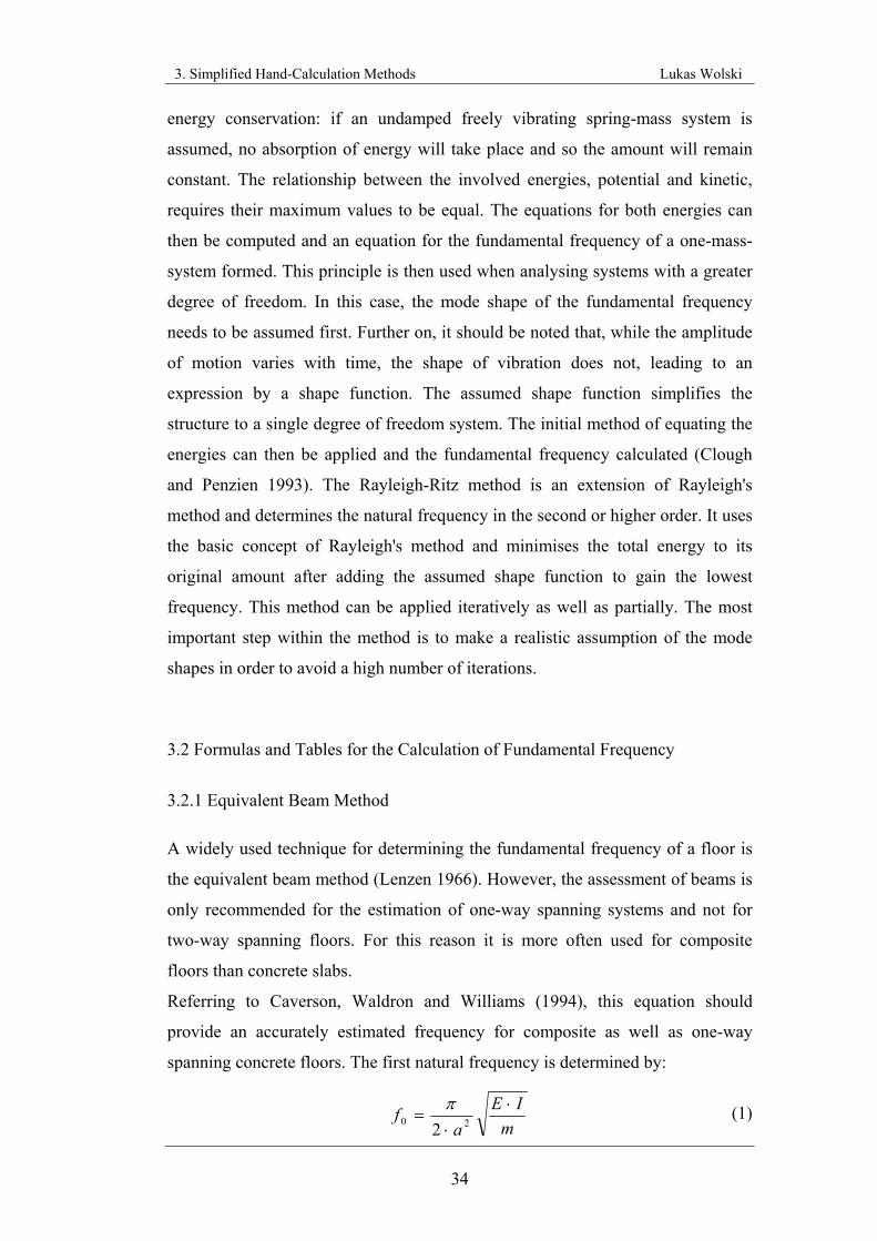
3. Simplified Hand-Calculation Methods Lukas Wolski
34
mIE
af ⋅
⋅= 20 2
π
energy conservation: if an undamped freely vibrating spring-mass system is
assumed, no absorption of energy will take place and so the amount will remain
constant. The relationship between the involved energies, potential and kinetic,
requires their maximum values to be equal. The equations for both energies can
then be computed and an equation for the fundamental frequency of a one-mass-
system formed. This principle is then used when analysing systems with a greater
degree of freedom. In this case, the mode shape of the fundamental frequency
needs to be assumed first. Further on, it should be noted that, while the amplitude
of motion varies with time, the shape of vibration does not, leading to an
expression by a shape function. The assumed shape function simplifies the
structure to a single degree of freedom system. The initial method of equating the
energies can then be applied and the fundamental frequency calculated (Clough
and Penzien 1993). The Rayleigh-Ritz method is an extension of Rayleigh's
method and determines the natural frequency in the second or higher order. It uses
the basic concept of Rayleigh's method and minimises the total energy to its
original amount after adding the assumed shape function to gain the lowest
frequency. This method can be applied iteratively as well as partially. The most
important step within the method is to make a realistic assumption of the mode
shapes in order to avoid a high number of iterations.
3.2 Formulas and Tables for the Calculation of Fundamental Frequency
3.2.1 Equivalent Beam Method
A widely used technique for determining the fundamental frequency of a floor is
the equivalent beam method (Lenzen 1966). However, the assessment of beams is
only recommended for the estimation of one-way spanning systems and not for
two-way spanning floors. For this reason it is more often used for composite
floors than concrete slabs.
Referring to Caverson, Waldron and Williams (1994), this equation should
provide an accurately estimated frequency for composite as well as one-way
spanning concrete floors. The first natural frequency is determined by:
(1)
3. Simplified Hand-Calculation Methods Lukas Wolski
35
3.2.2 Equivalent Plate Approach
In addition to the equivalent beam method only applicable to one-way spanning
concrete slabs, Williams and Waldron (1994) as well as Jeary (1997) presented an
equation for the fundamental frequency of simply supported two-way spanning
slabs. Thanks to the influence of all three dimensions and the flexure rigidity of
the plate D, it incorporates biaxial slab properties and provides good solutions.
(2)
3.2.3 Concrete Society Method
Another calculation procedure for biaxial slabs was proposed by the Concrete
Society (2005). As with the equivalent plate approach, it uses an approximation of
the equivalent beam method and considers the increased stiffness of a two-way
spanning floor. This leads to two independent orthogonal modes occurring for
both directions individually. The lower of both natural frequencies can be
considered as the fundamental frequency for this slab. A general advantage of this
method is its multifarious application to different types of slabs including solid,
ribbed and waffle, and its additional consideration of several bays for each
direction. However, the following equations are just presented for solid slabs in
one direction (x-direction). The characteristics of the second direction mode are
determined by interchanging the x- and y-subscripts in these equations.
The first step is to define the effective aspect ration of the slab by:
(3)
Afterwards it is necessary to calculate the modification factor kx:
(4)
211
xxk
λ+=
41
⎟⎟⎠
⎞⎜⎜⎝
⎛=
x
y
y
xxx EI
EIl
lnλ
⎟⎟⎠
⎞⎜⎜⎝
⎛+= 220 2 yx llm
Df 11 π
3. Simplified Hand-Calculation Methods Lukas Wolski
36
( )⎟⎟⎟⎟
⎠
⎞
⎜⎜⎜⎜
⎝
⎛ +−−=
2
11'' yx
bxxx
nnffff
The natural frequency for slabs with perimeter supports is:
(5)
For slabs without perimeter supports, the latter equation has to be modified by
calculation of an additional frequency fb:
(6)
The final natural frequency can now be obtained by:
(7)
3.2.4 Static Deflection Method
As seen in paragraph 3.1, it is possible to calculate the natural frequency by aid of
the kinetic and potential energy within the structure. As a result of the associations
of both, kinetic energy with the motion of mass and potential energy with the
strain energy stored in the elastic structure during deformation, a relationship
between the natural frequency and the deflection of a structure exists. This
relationship can be used to calculate the fundamental frequency for structures
whose static deflection is known. The derivation of an equation for an example of
the spring-mass-system demonstrates the relationship well. The static deflection
of a mass attached on a spring is given by:
(8)
4'
2
y
yxx ml
EIkf π
=
kgm
S⋅
=δ
4
4
4
1
2
xy
yx
x
x
b
lEIlEI
mlEI
f
+
=
π
3. Simplified Hand-Calculation Methods Lukas Wolski
37
The natural frequency is already known as:
(9)
Now it is possible to incorporate equation 3.4.1 into equation 3.1 which gives:
(10)
The final equation shows that only the acceleration due to gravity and the
maximum static deflection are required to obtain the fundamental frequency. But
due to an additional factor, the length of span is involved now, this method should
be more accurate than that of equation 1. Of course, this depends on the accuracy
of the estimated static deflection but the higher amount of necessary data used in
the calculation of static deflection allows this initial conclusion.
A modified version of this method was published by Blenvis (1979), who used the
expression derived by Mazumdar (1971) and modified by Jones (1975) for
calculating fundamental frequency. These earlier authors developed a method to
estimate natural frequency aided by the constant deflection lines of an element.
Although this equation was developed for clamped elliptic plates, it also predicts
the first frequency of plates of various shapes and boundary conditions. The new
equation is now:
(11)
3.2.5 Approximation Presented by Hearmon
Hearmon (1959) presented approximations for the estimation of rectangular
orthotropic plates using the already derived expressions from Warburton (1954)
and extending them to orthotropic plates with a combination of clamped or
mkf
π21
=
S
gfδπ2
277.1=
S
gfδπ2
1=
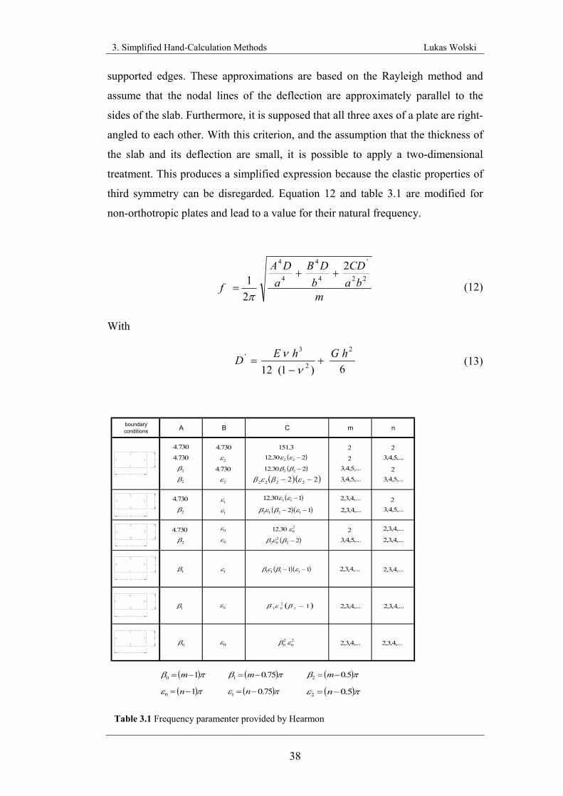
3. Simplified Hand-Calculation Methods Lukas Wolski
38
supported edges. These approximations are based on the Rayleigh method and
assume that the nodal lines of the deflection are approximately parallel to the
sides of the slab. Furthermore, it is supposed that all three axes of a plate are right-
angled to each other. With this criterion, and the assumption that the thickness of
the slab and its deflection are small, it is possible to apply a two-dimensional
treatment. This produces a simplified expression because the elastic properties of
third symmetry can be disregarded. Equation 12 and table 3.1 are modified for
non-orthotropic plates and lead to a value for their natural frequency.
(12) With
(13)
boundary conditions A B C m n
20 30.12 ε
2730.4 730.4730.4
730.4
730.4
2ε
1ε
730.42β
1β
1β
0β
0ε
,...5,4,3
,...4,3,2
3.151( )2 30.12 22 −εε
( )2 30.12 22 −ββ
( ) ( )2 2 2222 −− εβεβ
( )1 30.12 11 −εε
( )( )1 2 1212 −− εβεβ
( )2 2202 −βεβ
( )( )1 1 1111 −− εβεβ
( )11201 −βεβ
20
20 εβ
2
2
2
2
2
,...5,4,3
,...5,4,3 ,...5,4,3
,...5,4,3
,...4,3,2
,...4,3,2
,...4,3,2
,...4,3,2 ,...4,3,2
,...4,3,2
,...4,3,2 ,...4,3,2
,...4,3,2
2β
2β
2β
2ε
1ε
1ε
0ε
0ε
0ε
,...5,4,3
( )πβ 10 −= m ( )πβ 75.01 −= m ( )πβ 5.02 −= m
( )πε 10 −= n ( )πε 75.01 −= n ( )πε 5.02 −= n
Table 3.1 Frequency paramenter provided by Hearmon
mba
CDb
DBa
DA
f22
'
4
4
4
4 2
21
++=
π
6
)1( 12 2
2
3' hGhED +
−=
νν
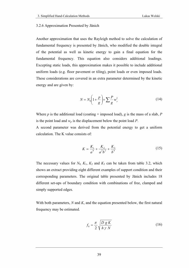
3. Simplified Hand-Calculation Methods Lukas Wolski
39
3.2.6 Approximation Presented by Jänich
Another approximation that uses the Rayleigh method to solve the calculation of
fundamental frequency is presented by Jänich, who modified the double integral
of the potential as well as kinetic energy to gain a final equation for the
fundamental frequency. This equation also considers additional loadings.
Excepting static loads, this approximation makes it possible to include additional
uniform loads (e.g. floor pavement or tiling), point loads or even imposed loads.
These considerations are covered in an extra parameter determined by the kinetic
energy and are given by:
(14)
Where p is the additional load (coating + imposed load), g is the mass of a slab, P
is the point load and wp is the displacement below the point load P.
A second parameter was derived from the potential energy to get a uniform
calculation. The K value consists of:
(15)
The necessary values for N0, K1, K2 and K3 can be taken from table 3.2, which
shows an extract providing eight different examples of support condition and their
corresponding parameters. The original table presented by Jänich includes 18
different set-ups of boundary condition with combinations of free, clamped and
simply supported edges.
With both parameters, N and K, and the equation presented below, the first natural
frequency may be estimated.
(16)
∑+⎟⎟⎠
⎞⎜⎜⎝
⎛+= 2
0 1P
wgP
gpNN
43
222
41
bK
baK
aKK ++=
Nhg KDf
γ
π20 =
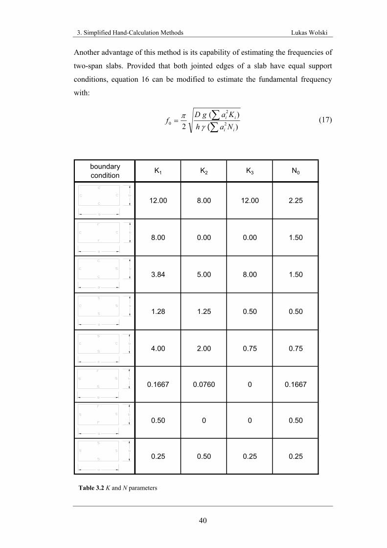
3. Simplified Hand-Calculation Methods Lukas Wolski
40
Another advantage of this method is its capability of estimating the frequencies of
two-span slabs. Provided that both jointed edges of a slab have equal support
conditions, equation 16 can be modified to estimate the fundamental frequency
with:
(17)
boundary condition
K1 K2 K3 N0
12.00 8.00 12.00 2.25
8.00 0.00 0.00 1.50
3.84 5.00 8.00 1.50
1.28 1.25 0.50 0.50
4.00 2.00 0.75 0.75
0.1667 0.0760 0 0.1667
0.50 0 0 0.50
0.25 0.50 0.25 0.25
))(
2 2
2
0ii
ii
NahKag D
f∑∑=
( γ
π
Table 3.2 K and N parameters
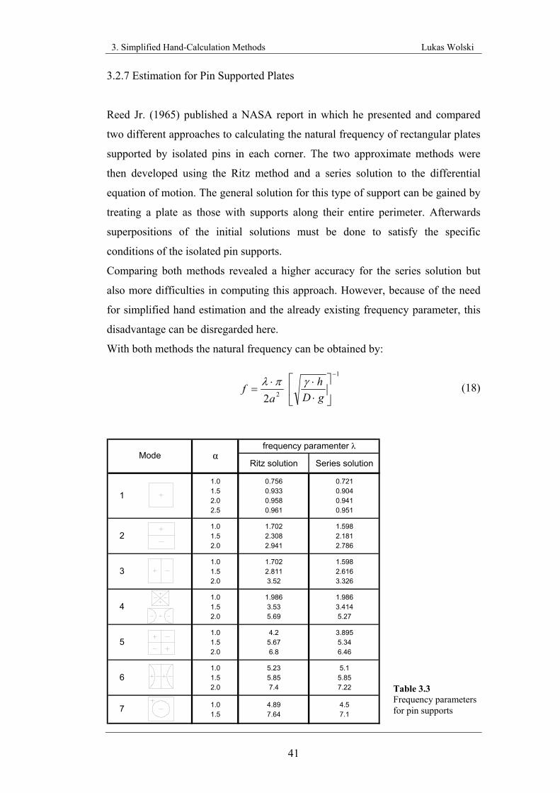
3. Simplified Hand-Calculation Methods Lukas Wolski
41
3.2.7 Estimation for Pin Supported Plates
Reed Jr. (1965) published a NASA report in which he presented and compared
two different approaches to calculating the natural frequency of rectangular plates
supported by isolated pins in each corner. The two approximate methods were
then developed using the Ritz method and a series solution to the differential
equation of motion. The general solution for this type of support can be gained by
treating a plate as those with supports along their entire perimeter. Afterwards
superpositions of the initial solutions must be done to satisfy the specific
conditions of the isolated pin supports.
Comparing both methods revealed a higher accuracy for the series solution but
also more difficulties in computing this approach. However, because of the need
for simplified hand estimation and the already existing frequency parameter, this
disadvantage can be disregarded here.
With both methods the natural frequency can be obtained by:
(18)
Ritz solution Series solution
1.0 0.756 0.7211.5 0.933 0.9042.0 0.958 0.9412.5 0.961 0.951
1.0 1.702 1.5981.5 2.308 2.1812.0 2.941 2.786
1.0 1.702 1.5981.5 2.811 2.6162.0 3.52 3.326
1.0 1.986 1.9861.5 3.53 3.4142.0 5.69 5.27
1.0 4.2 3.8951.5 5.67 5.342.0 6.8 6.46
1.0 5.23 5.11.5 5.85 5.852.0 7.4 7.22
1.0 4.89 4.51.5 7.64 7.1
αfrequency paramenter λ
4
5
Mode
6
7
1
2
3
2
1
2
−
⎥⎦
⎤⎢⎣
⎡
⋅⋅⋅
=gDh
af γπλ
Table 3.3 Frequency parameters for pin supports
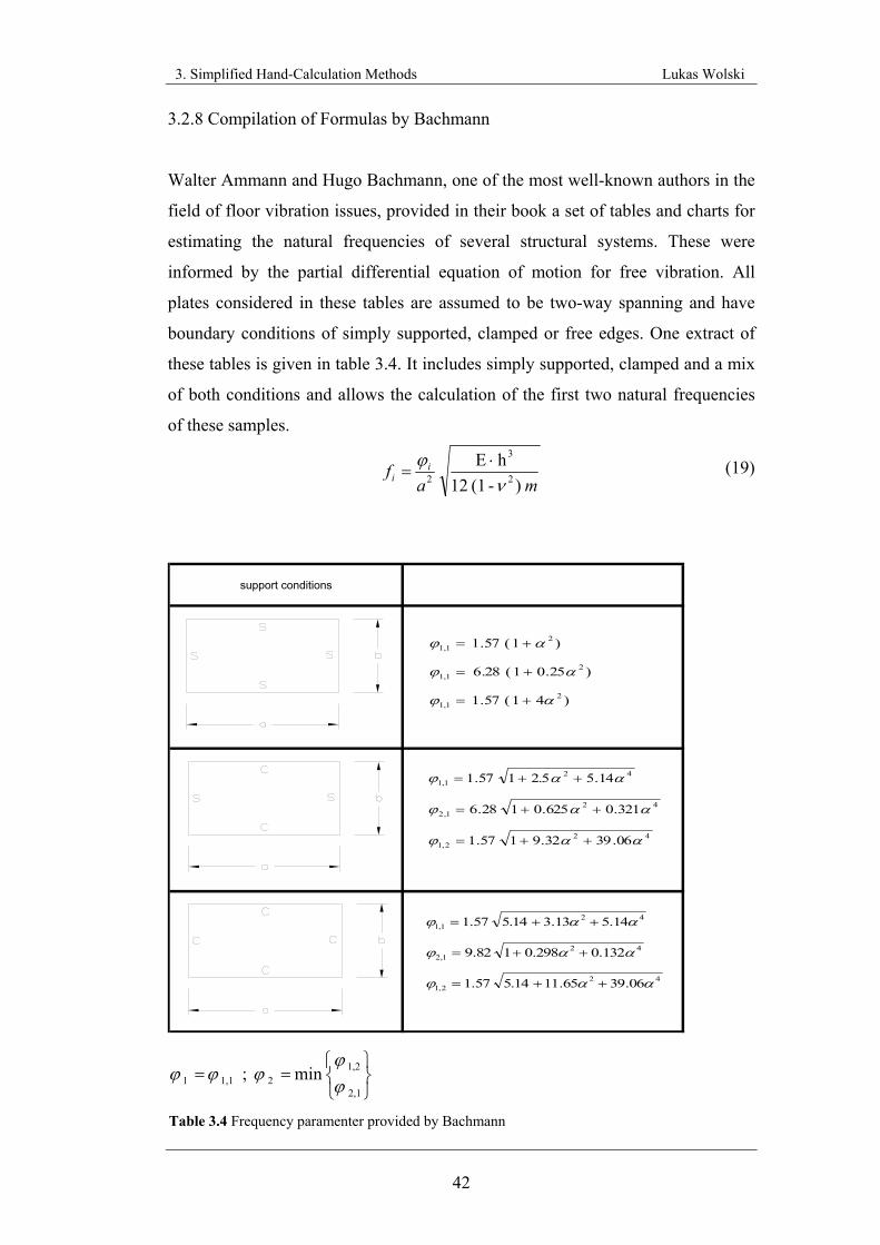
3. Simplified Hand-Calculation Methods Lukas Wolski
42
3.2.8 Compilation of Formulas by Bachmann
Walter Ammann and Hugo Bachmann, one of the most well-known authors in the
field of floor vibration issues, provided in their book a set of tables and charts for
estimating the natural frequencies of several structural systems. These were
informed by the partial differential equation of motion for free vibration. All
plates considered in these tables are assumed to be two-way spanning and have
boundary conditions of simply supported, clamped or free edges. One extract of
these tables is given in table 3.4. It includes simply supported, clamped and a mix
of both conditions and allows the calculation of the first two natural frequencies
of these samples.
(19)
support conditions
422,1
421,2
421,1
06.3932.91 57.1
321.0625.01 28.6
14.52.51 57.1
ααϕ
ααϕ
ααϕ
++=
++=
++=
422,1
421,2
421,1
06.3965.115.14 57.1
132.0298.01 82.9
14.513.35.14 57.1
ααϕ
ααϕ
ααϕ
++=
++=
++=
)41 ( 57.1
)25.01 ( .286
)1 ( 57.1
21,1
21,1
21,1
αϕ
αϕ
αϕ
+=
+=
+=
min ; 2,1
1,2 2 1,1 1
⎭⎬⎫
⎩⎨⎧
==ϕϕ
ϕϕϕ
Table 3.4 Frequency paramenter provided by Bachmann
maf i
i )-(1 12hE 2
3
2 νϕ ⋅
=
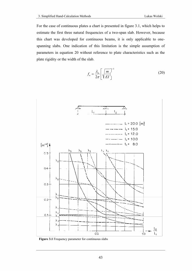
3. Simplified Hand-Calculation Methods Lukas Wolski
43
For the case of continuous plates a chart is presented in figure 3.1, which helps to
estimate the first three natural frequencies of a two-span slab. However, because
this chart was developed for continuous beams, it is only applicable to one-
spanning slabs. One indication of this limitation is the simple assumption of
parameters in equation 20 without reference to plate characteristics such as the
plate rigidity or the width of the slab.
(20)
Figure 3.1 Frequency parameter for continuous slabs
1
2
−
⎥⎦
⎤⎢⎣
⎡=
EImf n
n πλ
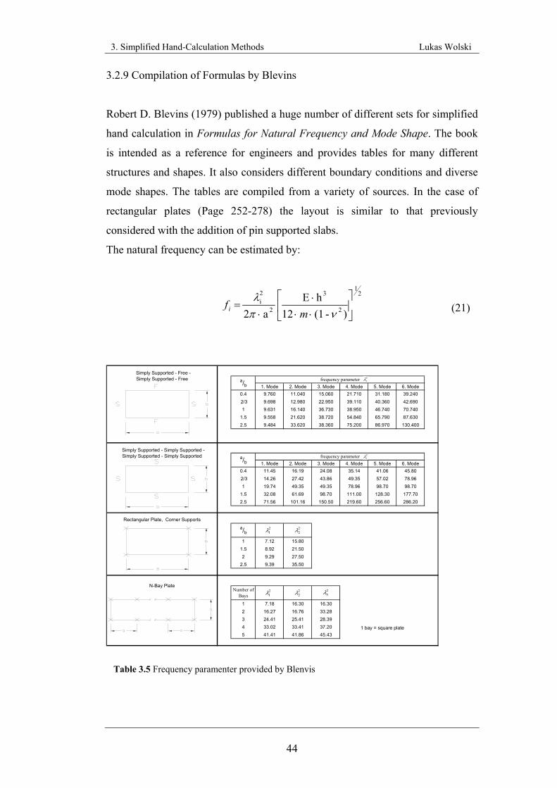
3. Simplified Hand-Calculation Methods Lukas Wolski
44
3.2.9 Compilation of Formulas by Blevins
Robert D. Blevins (1979) published a huge number of different sets for simplified
hand calculation in Formulas for Natural Frequency and Mode Shape. The book
is intended as a reference for engineers and provides tables for many different
structures and shapes. It also considers different boundary conditions and diverse
mode shapes. The tables are compiled from a variety of sources. In the case of
rectangular plates (Page 252-278) the layout is similar to that previously
considered with the addition of pin supported slabs.
The natural frequency can be estimated by:
(21)
1. Mode 2. Mode 3. Mode 4. Mode 5. Mode 6. Mode0.4 9.760 11.040 15.060 21.710 31.180 39.2402/3 9.698 12.980 22.950 39.110 40.360 42.6901 9.631 16.140 36.730 38.950 46.740 70.740
1.5 9.558 21.620 38.720 54.840 65.790 87.6302.5 9.484 33.620 38.360 75.200 86.970 130.400
1. Mode 2. Mode 3. Mode 4. Mode 5. Mode 6. Mode0.4 11.45 16.19 24.08 35.14 41.06 45.802/3 14.26 27.42 43.86 49.35 57.02 78.961 19.74 49.35 49.35 78.96 98.70 98.70
1.5 32.08 61.69 98.70 111.00 128.30 177.702.5 71.56 101.16 150.50 219.60 256.60 286.20
1 7.12 15.801.5 8.92 21.502 9.29 27.50
2.5 9.39 35.50
1 7.18 16.30 16.302 16.27 16.76 33.283 24.41 25.41 28.394 33.02 33.41 37.20 1 bay = square plate5 41.41 41.86 45.43
Simply Supported - Free - Simply Supported - Free
Simply Supported - Simply Supported -Simply Supported - Simply Supported
frequency parametera/b
a/bfrequency parameter
Rectangular Plate, Corner Supports
N-Bay PlateNumber of
Bays
a/b
2iλ
21λ
22λ
23λ
21λ
22λ
2iλ
21
2
3
2
2i
)-(1 12h E
a 2 ⎥
⎦
⎤⎢⎣
⎡
⋅⋅⋅
⋅=
νπλ
mfi
Table 3.5 Frequency paramenter provided by Blenvis
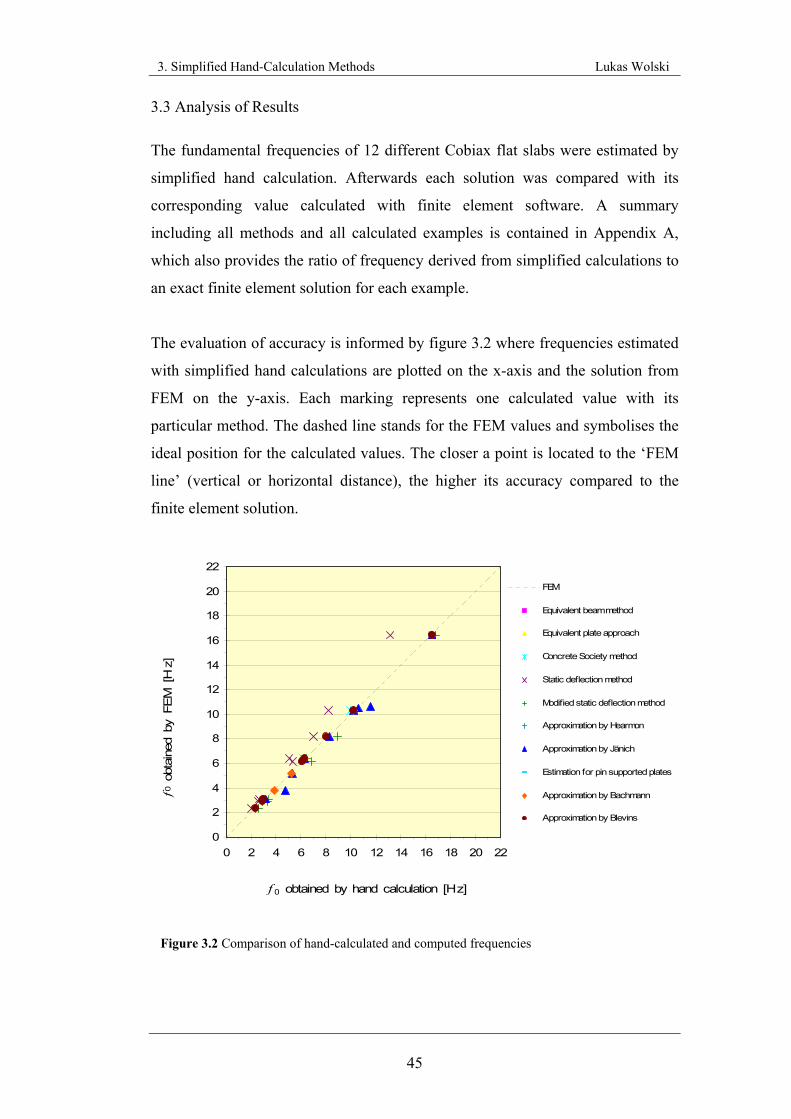
3. Simplified Hand-Calculation Methods Lukas Wolski
45
3.3 Analysis of Results
The fundamental frequencies of 12 different Cobiax flat slabs were estimated by
simplified hand calculation. Afterwards each solution was compared with its
corresponding value calculated with finite element software. A summary
including all methods and all calculated examples is contained in Appendix A,
which also provides the ratio of frequency derived from simplified calculations to
an exact finite element solution for each example.
The evaluation of accuracy is informed by figure 3.2 where frequencies estimated
with simplified hand calculations are plotted on the x-axis and the solution from
FEM on the y-axis. Each marking represents one calculated value with its
particular method. The dashed line stands for the FEM values and symbolises the
ideal position for the calculated values. The closer a point is located to the ‘FEM
line’ (vertical or horizontal distance), the higher its accuracy compared to the
finite element solution.
0
2
4
6
8
10
12
14
16
18
20
22
0 2 4 6 8 10 12 14 16 18 20 22
f 0 obtained by hand calculation [H z]
f0 o
btai
ned
by
FEM
[H
z]
FEM
Equivalent beam method
Equivalent plate approach
Concrete Society method
Static deflection method
Modified static deflection method
Approximation by Hearmon
Approximation by Jänich
Estimation for pin supported plates
Approximation by Bachmann
Approximation by Blevins
Figure 3.2 Comparison of hand-calculated and computed frequencies
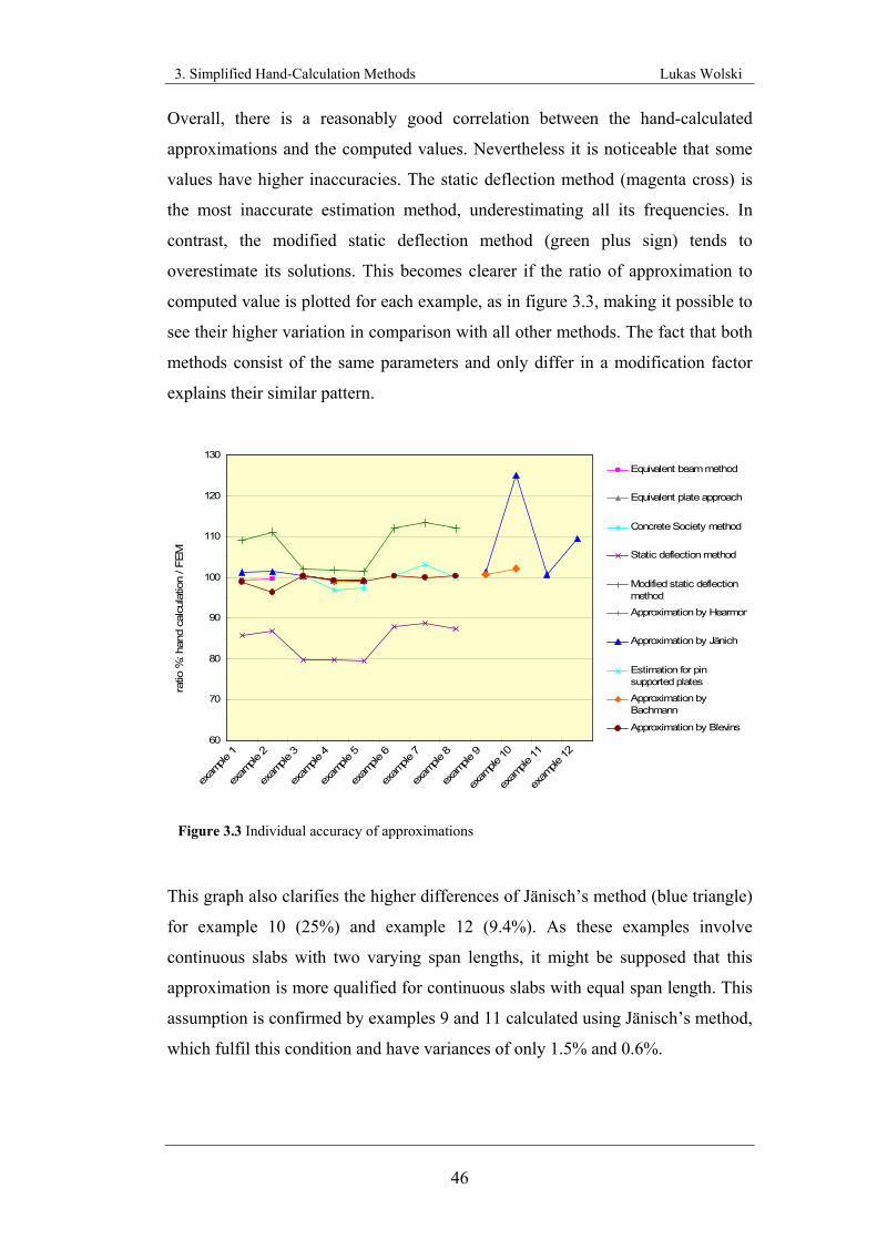
3. Simplified Hand-Calculation Methods Lukas Wolski
46
Overall, there is a reasonably good correlation between the hand-calculated
approximations and the computed values. Nevertheless it is noticeable that some
values have higher inaccuracies. The static deflection method (magenta cross) is
the most inaccurate estimation method, underestimating all its frequencies. In
contrast, the modified static deflection method (green plus sign) tends to
overestimate its solutions. This becomes clearer if the ratio of approximation to
computed value is plotted for each example, as in figure 3.3, making it possible to
see their higher variation in comparison with all other methods. The fact that both
methods consist of the same parameters and only differ in a modification factor
explains their similar pattern.
60
70
80
90
100
110
120
130
exam
ple 1
exam
ple 2
exam
ple 3
exam
ple 4
exam
ple 5
exam
ple 6
exam
ple 7
exam
ple 8
exam
ple 9
exam
ple 10
exam
ple 11
exam
ple 12
ratio
%: h
and
calc
ulat
ion
/ FEM
Equivalent beam method
Equivalent plate approach
Concrete Society method
Static deflection method
Modified static deflectionmethod
Approximation by Hearmon
Approximation by Jänich
Estimation for pinsupported plates
Approximation byBachmann
Approximation by Blevins
This graph also clarifies the higher differences of Jänisch’s method (blue triangle)
for example 10 (25%) and example 12 (9.4%). As these examples involve
continuous slabs with two varying span lengths, it might be supposed that this
approximation is more qualified for continuous slabs with equal span length. This
assumption is confirmed by examples 9 and 11 calculated using Jänisch’s method,
which fulfil this condition and have variances of only 1.5% and 0.6%.
Figure 3.3 Individual accuracy of approximations
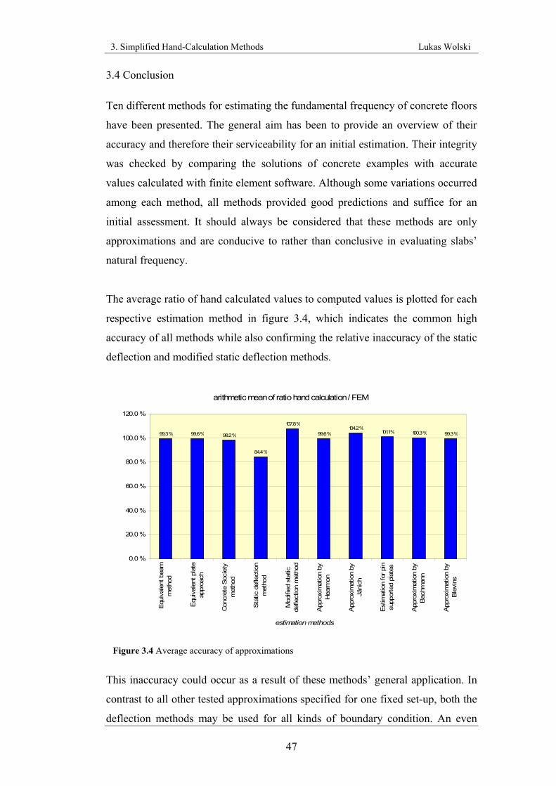
3. Simplified Hand-Calculation Methods Lukas Wolski
47
3.4 Conclusion
Ten different methods for estimating the fundamental frequency of concrete floors
have been presented. The general aim has been to provide an overview of their
accuracy and therefore their serviceability for an initial estimation. Their integrity
was checked by comparing the solutions of concrete examples with accurate
values calculated with finite element software. Although some variations occurred
among each method, all methods provided good predictions and suffice for an
initial assessment. It should always be considered that these methods are only
approximations and are conducive to rather than conclusive in evaluating slabs’
natural frequency.
The average ratio of hand calculated values to computed values is plotted for each
respective estimation method in figure 3.4, which indicates the common high
accuracy of all methods while also confirming the relative inaccuracy of the static
deflection and modified static deflection methods.
arithmetic mean of ratio hand calculation / FEM
99.6 % 98.2 %
84.4 %
107.8 %
99.6 %104.2 %
101.1 % 100.3 % 99.3 %99.3 %
0.0 %
20.0 %
40.0 %
60.0 %
80.0 %
100.0 %
120.0 %
Equ
ival
ent b
eam
met
hod
Equ
ival
ent p
late
appr
oach
Con
cret
e S
ocie
tym
etho
d
Sta
tic d
efle
ctio
nm
etho
d
Mod
ified
sta
ticde
flect
ion
met
hod
App
roxi
mat
ion
byH
earm
on
App
roxi
mat
ion
byJä
nich
Est
imat
ion
for p
insu
ppor
ted
plat
es
App
roxi
mat
ion
byB
achm
ann
App
roxi
mat
ion
byB
levi
ns
estimation methods
This inaccuracy could occur as a result of these methods’ general application. In
contrast to all other tested approximations specified for one fixed set-up, both the
deflection methods may be used for all kinds of boundary condition. An even
Figure 3.4 Average accuracy of approximations
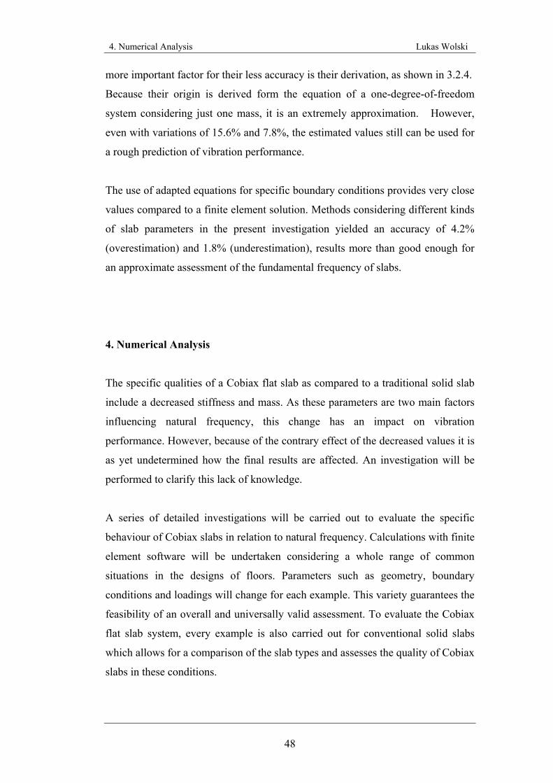
4. Numerical Analysis Lukas Wolski
48
more important factor for their less accuracy is their derivation, as shown in 3.2.4.
Because their origin is derived form the equation of a one-degree-of-freedom
system considering just one mass, it is an extremely approximation. However,
even with variations of 15.6% and 7.8%, the estimated values still can be used for
a rough prediction of vibration performance.
The use of adapted equations for specific boundary conditions provides very close
values compared to a finite element solution. Methods considering different kinds
of slab parameters in the present investigation yielded an accuracy of 4.2%
(overestimation) and 1.8% (underestimation), results more than good enough for
an approximate assessment of the fundamental frequency of slabs.
4. Numerical Analysis
The specific qualities of a Cobiax flat slab as compared to a traditional solid slab
include a decreased stiffness and mass. As these parameters are two main factors
influencing natural frequency, this change has an impact on vibration
performance. However, because of the contrary effect of the decreased values it is
as yet undetermined how the final results are affected. An investigation will be
performed to clarify this lack of knowledge.
A series of detailed investigations will be carried out to evaluate the specific
behaviour of Cobiax slabs in relation to natural frequency. Calculations with finite
element software will be undertaken considering a whole range of common
situations in the designs of floors. Parameters such as geometry, boundary
conditions and loadings will change for each example. This variety guarantees the
feasibility of an overall and universally valid assessment. To evaluate the Cobiax
flat slab system, every example is also carried out for conventional solid slabs
which allows for a comparison of the slab types and assesses the quality of Cobiax
slabs in these conditions.
4. Numerical Analysis Lukas Wolski
49
4.1 Software
Because this research was undertaken in collaboration with Cobiax Technologies
GmbH, Germany, special software was provided for the investigation, namely the
finite element software Tornow-Software, established in Germany since 1983.
The software is subdivided into several packages for individual scopes. For this
investigation the “FEM-Tripla” package, developed for the design of floor
systems, was applied. A big advantage here was its additional ‘Cobiax module’
(Figure 4.1), specially generated for the design of Cobiax flat slabs. After the
input of all necessary data, including thickness of the slab and ball diameter, the
corresponding decreasing of mass and stiffness are taken into consideration.
The package has different set-ups for investigating natural frequency and is
capable of calculating up to 10 natural frequencies using different approaches.
The following investigation considers the first three frequencies with the main
focus on fundamental frequency. Analysis of the natural frequencies is calculated
using the Lanczos algorithm, an iterative algorithm which employs the Lanczos
recursion. This is a process of defining or expressing a function or the solution to
a problem in terms of itself, by producing a recursive function. However, it is also
a very powerful solver and well known as an efficient method of finding
eigenvalues and eigenvectors of matrices. The Lanczos procedure is generally
Figure 4.1 Cobiax module
4. Numerical Analysis Lukas Wolski
50
used for large sparse matrices. Cullum and Willoughby (1985) summarised the
basic steps in any Lanczos procedure as shown below.
1. Transform a given ‘symmetric’ matrix A into a family of ‘symmetric’
tridiagonal matrices of varying sizes
2. Compute eigenvalues and eigenvectors of certain members of this
family
3. Take some or all of these eigenvalues as approximations to eigenvalues
of matrix A and map the corresponding eigenvectors of the tridiagonal
matrix into Ritz vectors for matrix A
4. Use these Ritz vectors as approximations to the eigenvectors of A
The accuracy of the calculated frequencies is set to 10-5 and is also improved by a
small and detailed mesh.
4.2 Verification of Software Accuracy
In terms of the obtained values’ accuracy, an initial test is carried out. A proof in
form of a comparison between Tornow-Software and a second finite element
software will clarify that Tornow-Software provides exact and accurate values.
For this purpose a slab was modelled with both types of software and its
fundamental frequency as well as its mode shape was calculated.
The used software is called RFEM 2.01 established by Dlubal Software. It is a
finite element software applicable for a wide range of tasks in structural
engineering.
The comparison consists of an example considering following parameters:
- One span solid slab
- All edges are simply supported
- 10m x 10m x 0.3m
- E = 28,300 N/mm² ; ν = 0.2 (C30/37)
- Imposed load q = 5.0 kN/m²
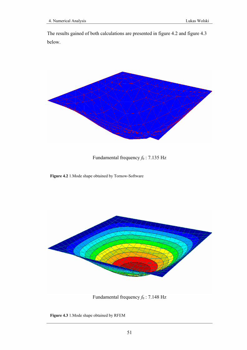
4. Numerical Analysis Lukas Wolski
51
The results gained of both calculations are presented in figure 4.2 and figure 4.3
below.
Fundamental frequency f0 : 7.135 Hz
Fundamental frequency f0 : 7.148 Hz
Figure 4.2 1.Mode shape obtained by Tornow-Software
Figure 4.3 1.Mode shape obtained by RFEM
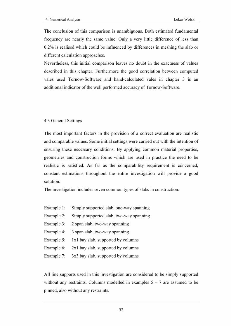
4. Numerical Analysis Lukas Wolski
52
The conclusion of this comparison is unambiguous. Both estimated fundamental
frequency are nearly the same value. Only a very little difference of less than
0.2% is realised which could be influenced by differences in meshing the slab or
different calculation approaches.
Nevertheless, this initial comparison leaves no doubt in the exactness of values
described in this chapter. Furthermore the good correlation between computed
vales used Tornow-Software and hand-calculated vales in chapter 3 is an
additional indicator of the well performed accuracy of Tornow-Software.
4.3 General Settings
The most important factors in the provision of a correct evaluation are realistic
and comparable values. Some initial settings were carried out with the intention of
ensuring these necessary conditions. By applying common material properties,
geometries and construction forms which are used in practice the need to be
realistic is satisfied. As far as the comparability requirement is concerned,
constant estimations throughout the entire investigation will provide a good
solution.
The investigation includes seven common types of slabs in construction:
Example 1: Simply supported slab, one-way spanning
Example 2: Simply supported slab, two-way spanning
Example 3: 2 span slab, two-way spanning
Example 4: 3 span slab, two-way spanning
Example 5: 1x1 bay slab, supported by columns
Example 6: 2x1 bay slab, supported by columns
Example 7: 3x3 bay slab, supported by columns
All line supports used in this investigation are considered to be simply supported
without any restraints. Columns modelled in examples 5 – 7 are assumed to be
pinned, also without any restraints.
4. Numerical Analysis Lukas Wolski
53
For each of these seven systems a range of different geometries are regarded.
These include changes in length of spans (6m-17m) and different width of spans
(4m-17m). The proper thickness was obtained with information offered on
Cobiax’s website (2006) and is provided in appendix C. One good resource here
was a diagram presenting amongst other things the interrelationship between slab
length and necessary thickness as well as ball diameter. Furthermore, a list of
already existing projects including floor geometries and ball diameters was used
to estimate an appropriate deck thickness. Depending on this thickness, which
ranges from between 30cm and 60cm, a proper Cobiax hollow sphere (Ø22.5cm-
Ø45cm) was used. A detailed description including all parameters is given in the
corresponding tables in appendix B.
As regards material properties, realistic terms are assumed by using a concrete
providing a quality of C30/37. As this is an averaged concrete quality, common in
design, it will deliver useful values. Referring to DIN1045-1, 9.1.7, its mean
Young's modulus is 28,300 N/mm². The second material quality, the Poisson ratio,
is supposed to be 0.2 for the concrete used in both types of slabs. According to
DIN 1055-1, 5.1, the unit weight for reinforced concrete is 25.0 kN/m³, the value
used to calculate the dead load. In addition, each slab is also loaded with
1.5 kN/m² to represent loading due to possible use of coating.
For further loadings it is important to consider the wide range of structures Cobiax
flat slabs are suitable for, including residences, offices and car parks. Thus, rather
than limiting this investigation to one design situation, as wide an application field
as possible is regarded. The imposed loads are staged according to this purpose. A
loading of 5.0 kN/m² is stepwise decreased by degrees of 25%, leading to further
loads of 3.75 kN/m², 2.50 kN/m², 1.25 kN/m², and finally 0 kN/m². In addition to
the dead load these five different loadings are used for each slab, providing a
variety of possible set-ups.
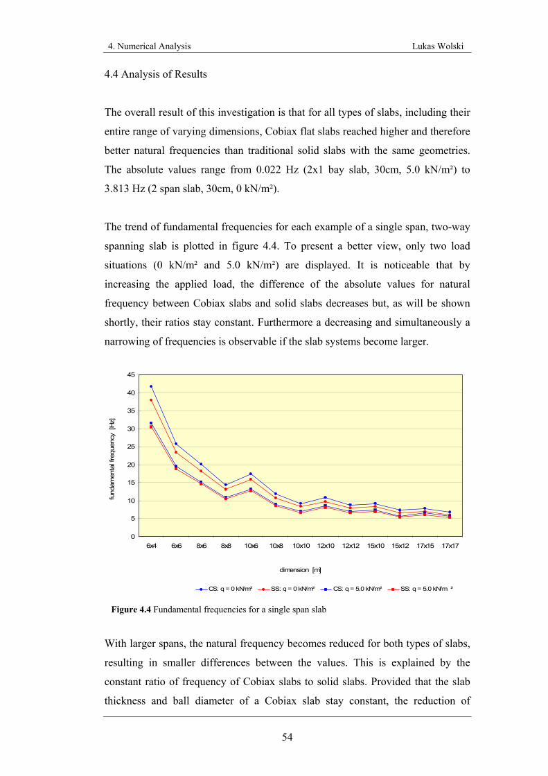
4. Numerical Analysis Lukas Wolski
54
4.4 Analysis of Results
The overall result of this investigation is that for all types of slabs, including their
entire range of varying dimensions, Cobiax flat slabs reached higher and therefore
better natural frequencies than traditional solid slabs with the same geometries.
The absolute values range from 0.022 Hz (2x1 bay slab, 30cm, 5.0 kN/m²) to
3.813 Hz (2 span slab, 30cm, 0 kN/m²).
The trend of fundamental frequencies for each example of a single span, two-way
spanning slab is plotted in figure 4.4. To present a better view, only two load
situations (0 kN/m² and 5.0 kN/m²) are displayed. It is noticeable that by
increasing the applied load, the difference of the absolute values for natural
frequency between Cobiax slabs and solid slabs decreases but, as will be shown
shortly, their ratios stay constant. Furthermore a decreasing and simultaneously a
narrowing of frequencies is observable if the slab systems become larger.
0
5
10
15
20
25
30
35
40
45
6x4 6x6 8x6 8x8 10x6 10x8 10x10 12x10 12x12 15x10 15x12 17x15 17x17
dimension [m]
fund
amen
tal f
requ
ency
[H
z]
CS: q = 0 kN/m² SS: q = 0 kN/m² CS: q = 5.0 kN/m² SS: q = 5.0 kN/m ²
With larger spans, the natural frequency becomes reduced for both types of slabs,
resulting in smaller differences between the values. This is explained by the
constant ratio of frequency of Cobiax slabs to solid slabs. Provided that the slab
thickness and ball diameter of a Cobiax slab stay constant, the reduction of
Figure 4.4 Fundamental frequencies for a single span slab
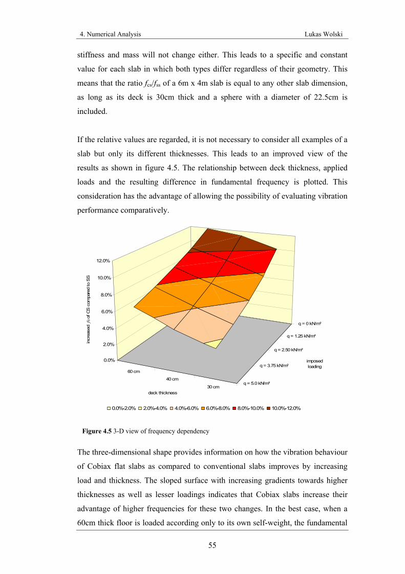
4. Numerical Analysis Lukas Wolski
55
stiffness and mass will not change either. This leads to a specific and constant
value for each slab in which both types differ regardless of their geometry. This
means that the ratio fcs/fss of a 6m x 4m slab is equal to any other slab dimension,
as long as its deck is 30cm thick and a sphere with a diameter of 22.5cm is
included.
If the relative values are regarded, it is not necessary to consider all examples of a
slab but only its different thicknesses. This leads to an improved view of the
results as shown in figure 4.5. The relationship between deck thickness, applied
loads and the resulting difference in fundamental frequency is plotted. This
consideration has the advantage of allowing the possibility of evaluating vibration
performance comparatively.
30 cm
40 cm
60 cm
q = 0 kN/m²
q = 1.25 kN/m²
q = 2.50 kN/m²
q = 3.75 kN/m²
q = 5.0 kN/m²
0.0%
2.0%
4.0%
6.0%
8.0%
10.0%
12.0%
incr
ease
d
f 0
of C
S c
ompa
red
to S
S
deck thickness
imposed loading
0.0%-2.0% 2.0%-4.0% 4.0%-6.0% 6.0%-8.0% 8.0%-10.0% 10.0%-12.0%
The three-dimensional shape provides information on how the vibration behaviour
of Cobiax flat slabs as compared to conventional slabs improves by increasing
load and thickness. The sloped surface with increasing gradients towards higher
thicknesses as well as lesser loadings indicates that Cobiax slabs increase their
advantage of higher frequencies for these two changes. In the best case, when a
60cm thick floor is loaded according only to its own self-weight, the fundamental
Figure 4.5 3-D view of frequency dependency
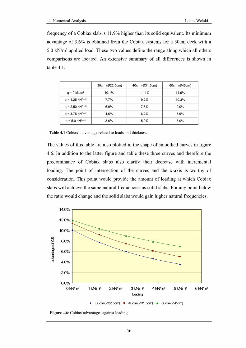
4. Numerical Analysis Lukas Wolski
56
frequency of a Cobiax slab is 11.9% higher than its solid equivalent. Its minimum
advantage of 3.6% is obtained from the Cobiax systems for a 30cm deck with a
5.0 kN/m² applied load. These two values define the range along which all others
comparisons are located. An extensive summary of all differences is shown in
table 4.1.
30cm (Ø22.5cm) 40cm (Ø31.5cm) 60cm (Ø45cm)
q = 0 kN/m² 10.1% 11.4% 11.9%
q = 1.25 kN/m² 7.7% 9.2% 10.3%
q = 2.50 kN/m² 6.0% 7.5% 9.0%
q = 3.75 kN/m² 4.6% 6.2% 7.9%
q = 5.0 kN/m² 3.6% 5.0% 7.0%
The values of this table are also plotted in the shape of smoothed curves in figure
4.6. In addition to the latter figure and table these three curves and therefore the
predominance of Cobiax slabs also clarify their decrease with incremental
loading. The point of intersection of the curves and the x-axis is worthy of
consideration. This point would provide the amount of loading at which Cobiax
slabs will achieve the same natural frequencies as solid slabs. For any point below
the ratio would change and the solid slabs would gain higher natural frequencies.
0.0%
2.0%
4.0%
6.0%
8.0%
10.0%
12.0%
14.0%
0 kN/m² 1 kN/m² 2 kN/m² 3 kN/m² 4 kN/m² 5 kN/m² 6 kN/m²loading
adva
ntag
e of
CS
30cm (Ø22.5cm) 40cm (Ø31.5cm) 60cm (Ø45cm)
Figure 4.6: Cobiax advantages against loading
Table 4.1 Cobiax’ advantage related to loads and thickness
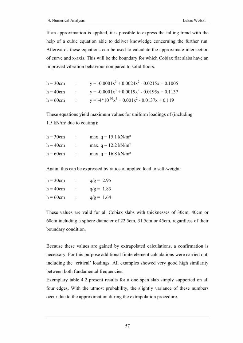
4. Numerical Analysis Lukas Wolski
57
If an approximation is applied, it is possible to express the falling trend with the
help of a cubic equation able to deliver knowledge concerning the further run.
Afterwards these equations can be used to calculate the approximate intersection
of curve and x-axis. This will be the boundary for which Cobiax flat slabs have an
improved vibration behaviour compared to solid floors.
h = 30cm : y = -0.0001x3 + 0.0024x2 - 0.0215x + 0.1005
h = 40cm : y = -0.0001x3 + 0.0019x2 - 0.0195x + 0.1137
h = 60cm : y = -4*10-05x3 + 0.001x2 - 0.0137x + 0.119
These equations yield maximum values for uniform loadings of (including
1.5 kN/m² due to coating):
h = 30cm : max. q = 15.1 kN/m²
h = 40cm : max. q = 12.2 kN/m²
h = 60cm : max. q = 16.8 kN/m²
Again, this can be expressed by ratios of applied load to self-weight:
h = 30cm : q/g = 2.95
h = 40cm : q/g = 1.83
h = 60cm : q/g = 1.64
These values are valid for all Cobiax slabs with thicknesses of 30cm, 40cm or
60cm including a sphere diameter of 22.5cm, 31.5cm or 45cm, regardless of their
boundary condition.
Because these values are gained by extrapolated calculations, a confirmation is
necessary. For this purpose additional finite element calculations were carried out,
including the ‘critical’ loadings. All examples showed very good high similarity
between both fundamental frequencies.
Exemplary table 4.2 present results for a one span slab simply supported on all
four edges. With the utmost probability, the slightly variance of these numbers
occur due to the approximation during the extrapolation procedure.
4. Numerical Analysis Lukas Wolski
58
CS SS Dimension f0 [Hz] f0 [Hz]
ratio fCS/fSS
8m x 8m x 0.3m 8.279 8.299 0.998 12m x 12m x 0.4m 5.843 5.740 1.018 17m x 17m x 0.6m 4.491 4.393 1.022
Another check of the accuracy is given in figure 4.7. This chart has plotted the
direct relationship of applied load and resulting fundamental frequency for both
types of slab. In this case, the values relate to a continuous slab with two equal
spans and the same length-width ratio. Like before, it is noticeable that the
obtained ‘critical’ value for 30cm slabs provides the highest accuracy which is
indicated by the very close intersection of both upper curves relating to the
predicted value (dashed line). But even if the approximation according to 40cm
and 60cm slabs are less accurate, the variance of 2% is still accurate enough to
evaluate the relationship between both types of slab.
0.00
2.00
4.00
6.00
8.00
10.00
12.00
14.00
16.00
0 2 4 6 8 10 12 14 16 18 20 22 24 26 28
applied load [kN]
fund
amen
tal f
requ
ency
[Hz]
CS: 8m x 8m x 30cm SS: 8m x 8m x 30cm CS: 12m x 12m x 40cm
SS: 12m x 12m x 40cm CS: 17m x 17m x 60cm SS: 17m x 17m x 60cm
The change in ratio between the different types of slab is caused by the decreasing
relevance the Cobiax slabs’ reduced self-weight. If the applied loadings are
similar to the self-weight, the reduction of approximately 30% mass is an
advantage for Cobiax slabs. However, once the applied loads increase, the self-
weight becomes just a small amount of the overall load and is therefore negligible.
If this occurs, the only difference on the part of Cobiax slabs is the reduced
stiffness which has a negative impact on the vibration behaviour and therefore
leads to lower natural frequencies.
Figure 4.7 Accuracy of ‘critical’ load for continuous slab
Table 4.2 Accuracy of ‘critical’ load for one span slab
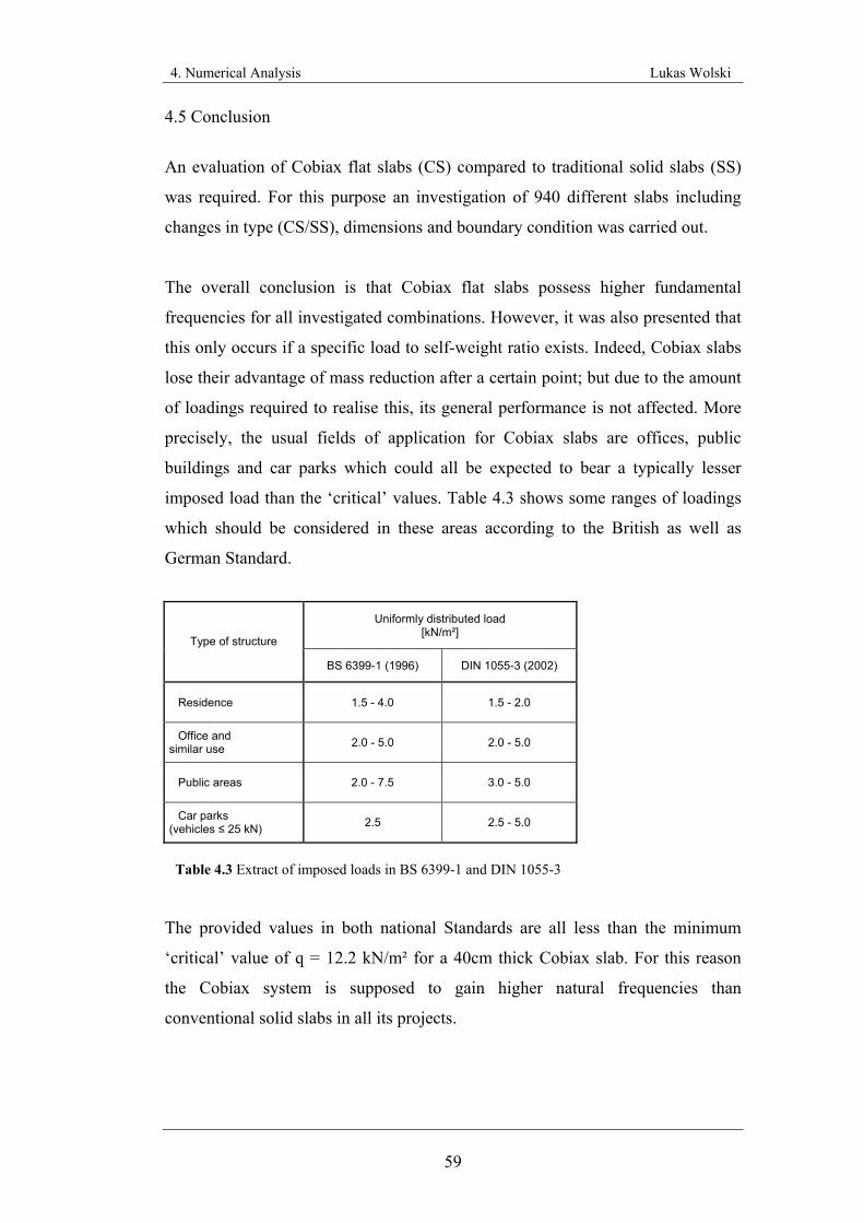
4. Numerical Analysis Lukas Wolski
59
4.5 Conclusion
An evaluation of Cobiax flat slabs (CS) compared to traditional solid slabs (SS)
was required. For this purpose an investigation of 940 different slabs including
changes in type (CS/SS), dimensions and boundary condition was carried out.
The overall conclusion is that Cobiax flat slabs possess higher fundamental
frequencies for all investigated combinations. However, it was also presented that
this only occurs if a specific load to self-weight ratio exists. Indeed, Cobiax slabs
lose their advantage of mass reduction after a certain point; but due to the amount
of loadings required to realise this, its general performance is not affected. More
precisely, the usual fields of application for Cobiax slabs are offices, public
buildings and car parks which could all be expected to bear a typically lesser
imposed load than the ‘critical’ values. Table 4.3 shows some ranges of loadings
which should be considered in these areas according to the British as well as
German Standard.
Uniformly distributed load [kN/m²]
Type of structure
BS 6399-1 (1996) DIN 1055-3 (2002)
Residence 1.5 - 4.0 1.5 - 2.0
Office and similar use 2.0 - 5.0 2.0 - 5.0
Public areas 2.0 - 7.5 3.0 - 5.0
Car parks (vehicles ≤ 25 kN) 2.5 2.5 - 5.0
The provided values in both national Standards are all less than the minimum
‘critical’ value of q = 12.2 kN/m² for a 40cm thick Cobiax slab. For this reason
the Cobiax system is supposed to gain higher natural frequencies than
conventional solid slabs in all its projects.
Table 4.3 Extract of imposed loads in BS 6399-1 and DIN 1055-3
5. Conclusions and Recommendations Lukas Wolski
60
5. Conclusions and Recommendations
5.1 General Conclusions
This research presents an overall view of natural frequency of concrete slabs in
structural engineering. Although it is a very large field of consideration, already
existing literature and research done in past provide good knowledge.
In case of human acceptance due to floor vibration a variety of recommendation is
available. By people like Reiher and Meister (1931), Wiss and Parmelee (1974)
or Brownjohn (2001) many investigations were carried out to improve the
knowledge of this topic. Nowadays, with help of the wide range of
recommendation, no significant complaints should occur. This conclusion is
supported by different case studies including annoying floor vibration, as shown
by Bachmann (1992) and Hanagan (2005). All cases describing vibration
complaints confirm very low natural frequencies of their floors and therefore a
high risk of perceptible motions.
Approximate hand-calculations presented in chapter three are a very well-know
area. Due to the fact that computer supported calculations were not available,
natural frequencies had to be estimated by hand calculations in the past. The high
amount of existing literature gives an easy access and considers common slab
types. In terms of accuracy of these simplifications performed comparisons of
hand-calculated values and solutions obtained by finite element software
confirmed their high quality. Even if some methods include small inaccuracy, it is
still possible to use them as an initial estimation. With all existing computer
software nowadays these methods are used for rough estimations anyway.
Chapter four containing the main issue of this research shows the improved
vibration performance of Cobiax flat slabs compared to conventional solid slabs.
A detailed investigation clarified the different effects of the reduced weight and
stiffness of Cobiax slabs. It is shown that due to their lower dead load Cobiax flat
slabs achieve higher natural frequencies for common practical use. However, with
an increasing of imposed load this advantage decreases and after a certain point
5. Conclusions and Recommendations Lukas Wolski
61
Cobiax slabs show lower and therefore worse natural frequencies. This change
happens because the ‘negative reduction’ of stiffness remains constant while after
increasing the ratio of applied load to self weight the ‘positive reduction’ of mass
decreases constantly until it becomes negligible.
An estimation of these ‘critical’ values indicates that because of the high amount
of imposed loadings necessary to achieve this change, the vibration behaviour is
still passable. All application areas Cobiax flat slabs used to focus show less
imposed load than the ‘critical’ values obtained.
5.2 Areas of Future Research
Because the fact that vibration performance of structures covers very large field of
consideration, further investigation are possible.
According to Lenzen (1966) one further important factor is the damping. A high
damping value is necessary to reduced floor vibration during its first cycles to avoid
human perception. Due to its reduced weight, the damping ratio is changed and leads to
other differences between Cobiax slabs and traditional solid slabs.
Another point which should be regarded is the thickness variety of Cobiax slabs.
Because each sphere diameter may be used for different thicknesses, the load reduction
changes as well. Again, this leads to individual ‘critical’ values for each slab-thickness
ratio. If, for example, a 22.5cm diameter ball is located inside a 40cm slab instead of a
30cm, the load reduction decreases from approximate 32% to 24%. According to
chapter four this would decrease the ‘critical’ value at which Cobiax slabs lose their
advantage compared to solid slabs.
References Lukas Wolski
62
References
Bachmann H. and Ammann W. (1987) Vibration in structures: Induced by man
and machines, International Association for Bridge and Structural Engineering
(IABSE)
Bachmann H. (1992) Case studies of structures with man-induced vibration,
Journal of Structural Engineering, 118(3), 631-647
Bachmann H. et al. (1995) Vibration problems in structures: practical guidelines,
Brinkhäuser Verlag
Bilbao S. (2002) Timoshenko's beam equations
http://ccrma.stanford.edu/~bilbao/master/node163.html [28 August 2006]
Blevins R.D. (1979) Formulas for natural frequency and mode shape, Krieger
Publishing Company
Bolton A. (1978) Natural frequencies of structures for designers,
The Structural Engineer, 56A(9), 245-253
Bolton A. (1994) Structural dynamics in practice: A guide for professional
engineers, McGraw-Hill
British Standards Institution (1992) BS 6472, Guide to evaluation of human
exposure to vibration in buildings (1 Hz to 80 Hz)
British Standards Institution (1996) BS 6399-1 Loading for buildings;
Part 1: Code of practice for dead and imposed loads
Brownjohn J.M.W. (2001) Energy dissipation from vibrating floor slabs due to
human structure interaction, Shock and Vibration, 8(6), 315-323
Clough R.W. and Penzien J. (1993) Dynamics of structures, 2nd edn. McGraw-Hill
References Lukas Wolski
63
Cobiax (2004) Planungshilfe: Cobiax Flachdecken, Cobiax Technologies AG
Cobiax (2006) Steifigkeitsfaktoren zur Berücksichtigung der Verminderung durch
Hohlkörper, Cobiax Technologies AG
Cobiax (2006) Lightweight solutions in concrete
http://www.cobiax.com [28 August 2006]
Concrete Society Working Party (2005) Post-tensioned concrete floor; Design
handbook, The Concrete Society
Cooney R.C. and King A.B. (1988) Serviceability criteria for buildings, Branz
study report, Building Research Association of New Zealand
Crist R.A. and Shaver J.R (1976) Deflection performance; Criteria for floors,
U.S. Department of Commerce, National Bureau of Standards
Cullum J.K. and Willoughby R.A. (1985) Lanczos algorithms for large
symmetric eigenvalues computations, Brickhäuser-Boston
Deutsches Institut für Normung (2001) DIN 1045-1, Tragwerke aus Beton,
Stahlbeton und Spannbeton; Teil 1: Bemessung und Konstruktion
Deutsches Institut für Normung (2002) DIN 1055-3, Einwirkungen auf
Tragwerke; Teil 3: Eigen- und Nutzlasten für Hochbauten
Deutsches Institut für Normung (2001) DIN 4150-1, Erschütterungen im
Bauwesen; Teil 1: Vorermittlung von Schwingungsgrößen
Deutsches Institut für Normung (1999) DIN 4150-2, Erschütterungen im
Bauwesen; Teil 2: Einwirkungen für Hochbauten
Elishakoff I.B. (1974) Vibration analysis of clamped square orthotropic plate,
American Institute of Aeronautics and Astronautics Journal, 12, 921-924
References Lukas Wolski
64
Emad El-Dardiry E. et al. (2002) Improving FE models of a long-span flat
concrete floor using natural frequency measurements, Computers and
Structures, 80, 2145–2156
Fisher J.M. and West M.A. (2001) Serviceability design considerations for low-
rise buildings, American Institute of Steel Construction
Griffin M.J. (1990) Handbook of human vibration, Academic Press Ltd.
Hanes R.M. (1970) Human sensitivity to whole-body vibration in urban
transportation systems: A literature review, Applied Physics Laboratory,
The Johns Hopkins University, Maryland.
Hearmon R.F.S. (1959) The frequency of flexural vibration of rectangular
orthotropic plates with clamped or supported edges, Journal of Applied
Mechanics, 26, 537-540
Jeary A. (1997) Designer’s guide to the dynamic response of structures,
E & FN Spon
Leissa A.W. (1973) The free vibration of rectangular plates, Journal of Sound and
Vibration, 31(3), 257-293
Linda M.and Hanagan L.M. (2005) Walking-Induced Floor Vibration Case
Studies, Journal of Architectural Engineering, 11(1), 14-18
Magrab E.B. (1977) Natural frequencies of elastically supported orthotropic
rectangular plates, Journal of the Acoustical Society of America, 61(1), 79-83
Mazumdar J. (1971) Transverse vibration of elastic plates by method of constant
deflection lines, Journal of Sound and Vibration, 18(2), 147-155
Mindlin R.D., Schacknow A. and Deresiewicz H. (1956) Flexural vibration of
rectangular plates, Journal of Applied Mechanics, 23, 430-436
References Lukas Wolski
65
Morrison J.B. (2006) Human response to vibration
http://www.sfu.ca [15 August 2006]
Osborne K.P. and Ellis B.R. (1990) Vibration design and testing of a long-span
lightweight floor, The Structural Engineer, 68(10), 181-186
Ove Arup & Partners (2004) Typical hospital floor; Vibration assessment,
Bubbledeck UK Ltd.
Pernica G. and Allen D.E. (1982) Floor vibration measurements in a shopping
centre, Canadian Journal of Civil Engineering, 9(2), 149-155
Pernica G. and Allen D.E. (1998) Control of Floor Vibration
http://irc.nrc-cnrc.gc.ca/pubs/ctus/22_e.html [11 August 2006]
Pfeffer K. (2002) Untersuchung zum Biege- und Durchstanztragverhalten von
zweiachsigen Hohlkörperdecken, VDI Verlag
Reed R.E.Jr. (1965) Comparison of methods in calculating frequencies of corner
supported rectangular plates, NASA Technical Note, NASA TN D-3030
Reiher H. and Meister F.J. (1931) Die Empfindlichkeit des Menschen gegen
Erschütterungen, Forschung auf dem Gebiet des Ingenieurwesens, 2(11),
381-386
Schnellenbach-Held M. (2003) Transverse force capability of the BubbleDeck,
Expert Report, Institute for Solid Construction, Technical University
Darmstadt
Tredgold T. (1828) Elementary Principles of Carpentry, 2nd Ed., J. Taylor
Warburton G.B. (1954) The vibration of rectangular plates, Proceedings of the
Institution of Mechanical Engineers, 168, 371-384
References Lukas Wolski
66
Weber B. (2002) Vorlesung Tragwerksdynamik, Institut für Baustatik und
Konstruktion, ETH Zürich
Wikipedia (2006) Rayleigh-Ritz-Prinzip
http://de.wikipedia.org/wiki/Rayleigh-Ritz-Prinzip [15 August 2006]
Wikipedia (2006) Rayleigh-Ritz method
http://en.wikipedia.org/wiki/Rayleigh-Ritz_method [15 August 2006]
Williams M.S. et al. (1993) Comparison of finite element and field test results for
the vibration of concrete floors, Int. Conf. on Structural Dynamics Modelling:
Test, Analysis and Correlation, Cranfield, 79-88
Wiss J.F. and Parmelee R.H. (1974) Human Perception of Transient Vibrations,
Journal of the Structural Division, ASCE, 100(ST4), 773-787
Young Benidickson V. (1993) Dealing with Excessive Floor Vibrations
http://irc.nrc-cnrc.gc.ca/pubs/cp/gen4_e.html [11 August 2006]
APPENDIX A Lukas Wolski
67
APPENDIX A
General Assumption ..............................................................................................68
Example 1 .............................................................................................................69
Example 2 .............................................................................................................71
Example 3 .............................................................................................................73
Example 4 .............................................................................................................76
Example 5 .............................................................................................................79
Example 6 .............................................................................................................82
Example 7 .............................................................................................................83
Example 8 .............................................................................................................86
Example 9 .............................................................................................................88
Example 10 ...........................................................................................................89
Example 11 ...........................................................................................................90
Example 12 ...........................................................................................................91
Summary of results ...............................................................................................92
APPENDIX A Lukas Wolski
68
General Assumption
The accuracy of the simplified hand calculation method proposed in chapter 3.2
was checked by the following example. To obtain comparable values, all methods
within each example dealt with the same set-up. It was assumed that all floors
were built using the Cobiax flat slab system. For the calculation of the
fundamental frequency no further loadings besides the self-weight were implied.
The material qualities were chosen for a C30/37 concrete with a Young's modulus
of 28 300 N/mm² and a density of 25 kN/m³. Depending on the geometry of each
system, the ball size diameter was 22.5cm or 31.5cm. For these two Cobiax flat
slab systems specific qualities such as stiffness reduction and deal load were
considered according to Appendix C. The boundary conditions included simply
supported one-way as well as two-way spanning floors, and pin supported 1x1
and 1x2 bay slabs. The only value which changed during this comparison was the
Poisson ratio. In general all examples used a Poisson ratio of 0.2, but because two
of the tables used for the estimation of pin supported slabs imply a Poisson ratio
of 0.3 these examples had to be modified and the Poisson ratio was increased.
Furthermore, it is important that every example used only suitable estimations for
its boundary condition. A comparison of specific methods to provide appropriate
solutions for different boundary conditions was waived on this occasion.
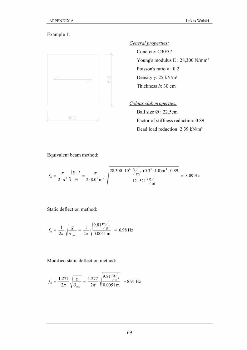
APPENDIX A Lukas Wolski
69
Example 1:
General properties:
Concrete: C30/37
Young's modulus E : 28,300 N/mm²
Poisson's ratio ν : 0.2
Density γ: 25 kN/m³
Thickness h: 30 cm
Cobiax slab properties:
Ball size Ø : 22.5cm
Factor of stiffness reduction: 0.89
Dead load reduction: 2.39 kN/m²
Equivalent beam method:
Hz .098
mkg521 12
0.89 1.0)m(0.3 m
N 10300,28
m8.0 2
2
432
6
2220 =⋅
⋅⋅⋅
⋅=
⋅⋅
=ππ
mIE
af
Static deflection method:
Hz 6.98 m 0051.0s
m 81.9
21
21
2
0 ===πδπ stat
gf
Modified static deflection method:
Hz 8.91 m 0051.0s
m 81.9
2277.1
2277.1
2
0 ===πδπ stat
gf
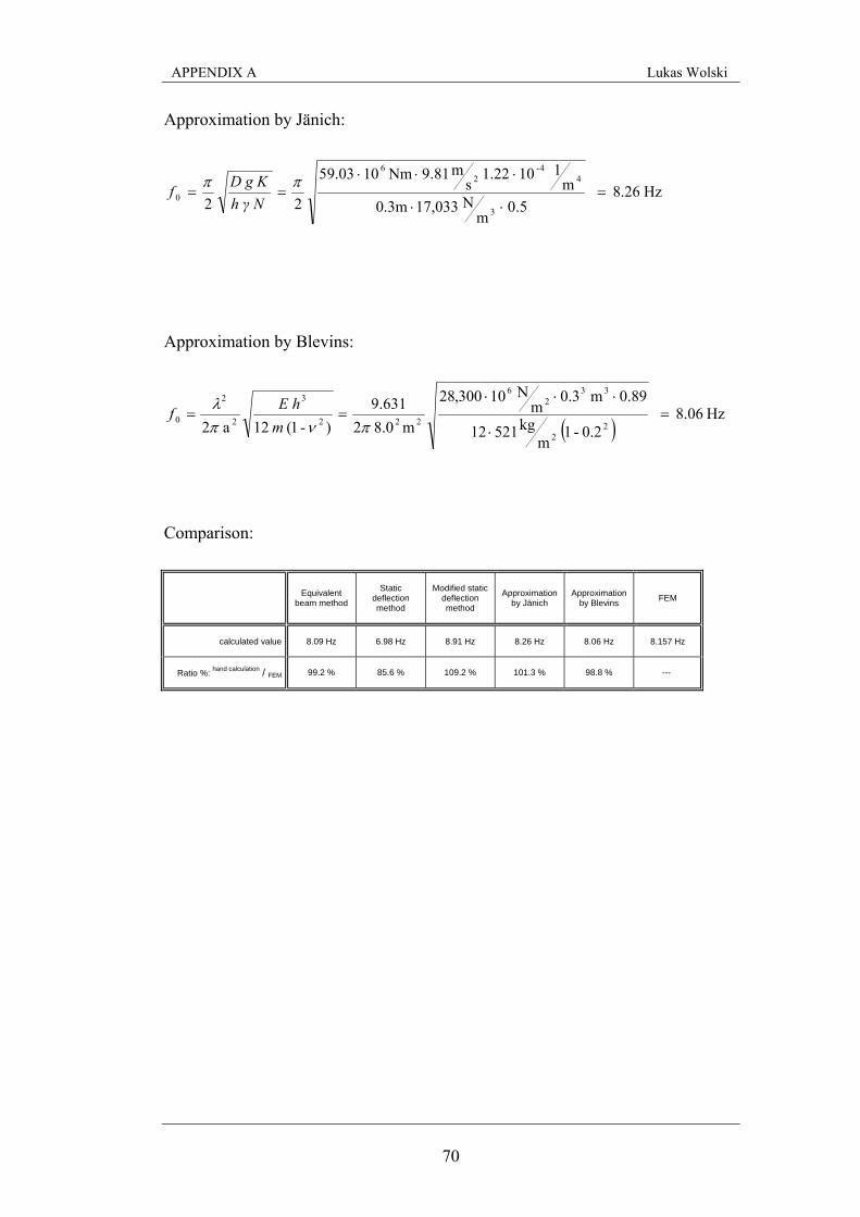
APPENDIX A Lukas Wolski
70
Approximation by Jänich:
Hz 8.26 5.0
mN 17,033 0.3m
m1101.22
sm81.9 Nm109.035
2 2 3
44-
26
0 =⋅⋅
⋅⋅⋅==ππ
N h γD g Kf
Approximation by Blevins:
( ) Hz 8.06
0.2-1 m
kg521 12
0.89 m 0.3 m
N10300,28
m8.0 2631.9
)-1( 12
a 2 22
332
6
222
3
2
2
0 =⋅
⋅⋅⋅==
πνπλ
mhEf
Comparison:
Equivalent beam method
Static deflection method
Modified static deflection method
Approximation by Jänich
Approximation by Blevins FEM
calculated value 8.09 Hz 6.98 Hz 8.91 Hz 8.26 Hz 8.06 Hz 8.157 Hz
Ratio %: hand calculation / FEM 99.2 % 85.6 % 109.2 % 101.3 % 98.8 % ---
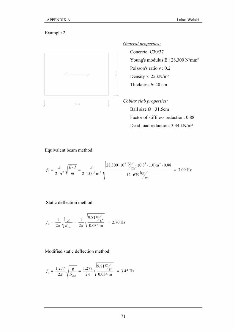
APPENDIX A Lukas Wolski
71
Example 2:
General properties:
Concrete: C30/37
Young's modulus E : 28,300 N/mm²
Poisson's ratio ν : 0.2
Density γ: 25 kN/m³
Thickness h: 40 cm
Cobiax slab properties:
Ball size Ø : 31.5cm
Factor of stiffness reduction: 0.88
Dead load reduction: 3.34 kN/m²
Equivalent beam method:
Hz .093
mkg679 12
0.88 1.0)m(0.3 m
N 10300,28
m15.0 2
2
432
6
2220 =⋅
⋅⋅⋅
⋅=
⋅⋅
=ππ
mIE
af
Static deflection method:
Hz 2.70 m 034.0s
m 81.9
21
21
2
0 ===πδπ stat
gf
Modified static deflection method:
Hz 3.45 m 034.0s
m 81.9
2277.1
2277.1
2
0 ===πδπ stat
gf
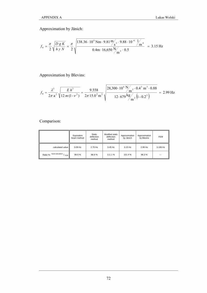
APPENDIX A Lukas Wolski
72
Approximation by Jänich:
Hz 3.15 5.0
mN 16,650 0.4m
m1109.88
sm81.9 Nm1036.138
2
2 3
46-
26
0 =⋅⋅
⋅⋅⋅⋅==π
γπ
Nhg KDf
Approximation by Blevins:
( ) Hz 2.99
0.2-1 m
kg679 12
0.88 m 0.4 m
N10300,28
m15.0 2558.9
)-1( 12
a 2 22
332
6
222
3
2
2
0 =⋅
⋅⋅⋅==
πνπλ
mhEf
Comparison:
Equivalent beam method
Static deflection method
Modified static deflection method
Approximation by Jänich
Approximation by Blevins FEM
calculated value 3.09 Hz 2.70 Hz 3.45 Hz 3.15 Hz 2.99 Hz 3.106 Hz
Ratio %: hand calculation / FEM 99.5 % 86.9 % 111.1 % 101.4 % 96.3 % ---
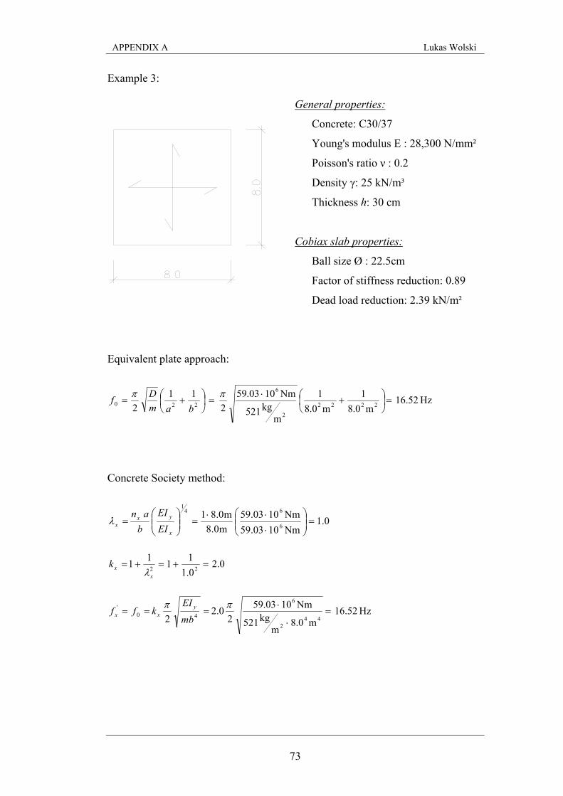
APPENDIX A Lukas Wolski
73
Example 3:
General properties:
Concrete: C30/37
Young's modulus E : 28,300 N/mm²
Poisson's ratio ν : 0.2
Density γ: 25 kN/m³
Thickness h: 30 cm
Cobiax slab properties:
Ball size Ø : 22.5cm
Factor of stiffness reduction: 0.89
Dead load reduction: 2.39 kN/m²
Equivalent plate approach:
Hz 16.52 m0.8
1m0.8
1
mkg 215
Nm1003.592
11 2 2222
2
6
220 =⎟⎠⎞
⎜⎝⎛ +
⋅=⎟
⎠⎞
⎜⎝⎛ +=
ππbam
Df
Concrete Society method:
0.1Nm1003.59Nm1003.59
m0.8m0.81
6
641
=⎟⎟⎠
⎞⎜⎜⎝
⎛
⋅⋅⋅
=⎟⎟⎠
⎞⎜⎜⎝
⎛=
x
yxx EI
EIb
anλ
0.20.11111 22 =+=+=
xxk
λ
Hz 16.52 m0.8
mkg521
Nm1003.592
2.0 2
44
2
6
40' =
⋅
⋅===
ππmbEI
kff yxx
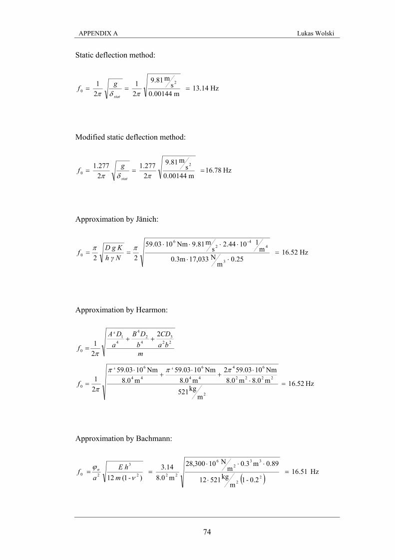
APPENDIX A Lukas Wolski
74
Static deflection method:
Hz 13.14 m 00144.0
sm 81.9
21
21
2
0 ===πδπ stat
gf
Modified static deflection method:
Hz 16.78 m 00144.0
sm 81.9
2277.1
2277.1
2
0 ===πδπ stat
gf
Approximation by Jänich:
Hz 16.52 25.0
mN 17,033 0.3m
m11044.2
sm81.9 Nm109.035
2 2 3
44-
26
0 =⋅⋅
⋅⋅⋅⋅==ππ
N h γD g Kf
Approximation by Hearmon:
Hz 16.52
mkg521
m0.8m0.8Nm1003.592
m0.8Nm1003.59
m0.8Nm1003.59
21
2
21
2
2222
64
44
6
44
6
0
223
42
4
41
0
44
4
=⋅⋅
+⋅
+⋅
=
++=
πππ
π
π
f
mba
CDb
DBa
DA
f
Approximation by Bachmann:
( )Hz 16.51
0.2-1 m
kg521 12
0.89 m0.3 m
N10300,28
m8.03.14
)-1( 12
22
332
6
222
3
20 =⋅
⋅⋅⋅==
νϕ
mhE
af n
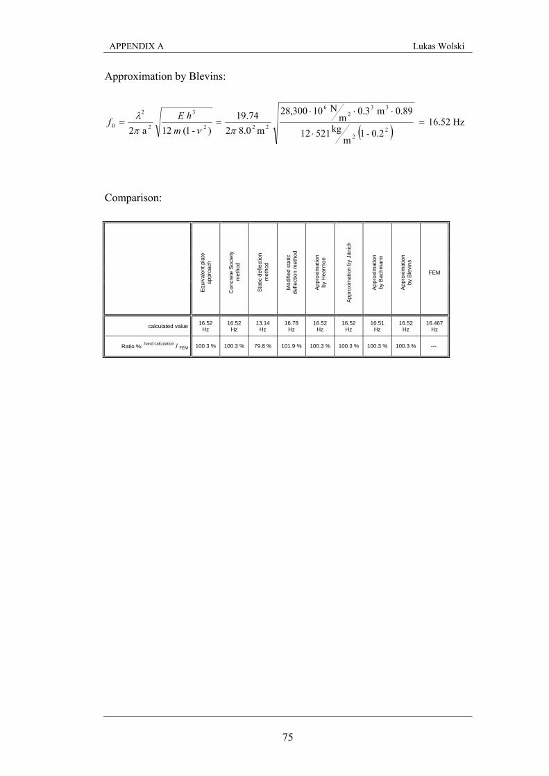
APPENDIX A Lukas Wolski
75
Approximation by Blevins:
( ) Hz 16.52
0.2-1 m
kg521 12
0.89 m 0.3 m
N10300,28
m8.0 274.19
)-1( 12
a 2 22
332
6
222
3
2
2
0 =⋅
⋅⋅⋅==
πνπλ
mhEf
Comparison:
Equ
ival
ent p
late
ap
proa
ch
Con
cret
e S
ocie
ty
met
hod
Sta
tic d
efle
ctio
n m
etho
d
Mod
ified
sta
tic
defle
ctio
n m
etho
d
App
roxi
mat
ion
by
Hea
rmon
App
roxi
mat
ion
by J
änic
h
App
roxi
mat
ion
by
Bac
hman
n
App
roxi
mat
ion
by
Ble
vins
FEM
calculated value 16.52 Hz
16.52 Hz
13.14 Hz
16.78 Hz
16.52 Hz
16.52 Hz
16.51 Hz
16.52 Hz
16.467 Hz
Ratio %: hand calculation / FEM 100.3 % 100.3 % 79.8 % 101.9 % 100.3 % 100.3 % 100.3 % 100.3 % ---
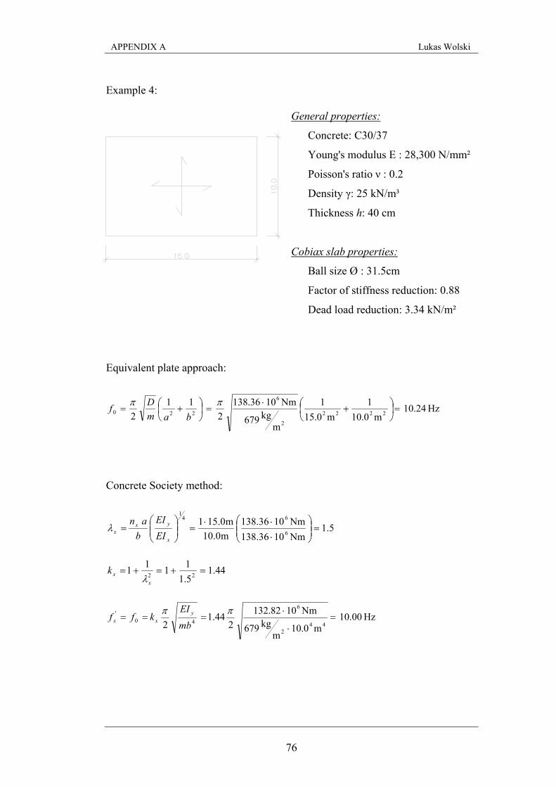
APPENDIX A Lukas Wolski
76
Example 4:
General properties:
Concrete: C30/37
Young's modulus E : 28,300 N/mm²
Poisson's ratio ν : 0.2
Density γ: 25 kN/m³
Thickness h: 40 cm
Cobiax slab properties:
Ball size Ø : 31.5cm
Factor of stiffness reduction: 0.88
Dead load reduction: 3.34 kN/m²
Equivalent plate approach:
Hz 10.24 m0.10
1m0.15
1
mkg 796
Nm1036.1382
11 2 2222
2
6
220 =⎟⎠⎞
⎜⎝⎛ +
⋅=⎟
⎠⎞
⎜⎝⎛ +=
ππbam
Df
Concrete Society method:
5.1Nm1036.381Nm1036.381
m0.10m0.151
6
641
=⎟⎟⎠
⎞⎜⎜⎝
⎛
⋅⋅⋅
=⎟⎟⎠
⎞⎜⎜⎝
⎛=
x
yxx EI
EIb
anλ
44.15.11111 22 =+=+=
xxk
λ
Hz 10.00 m0.10
mkg679
Nm1082.1322
1.44 2
44
2
6
40' =
⋅
⋅===
ππmbEI
kff yxx
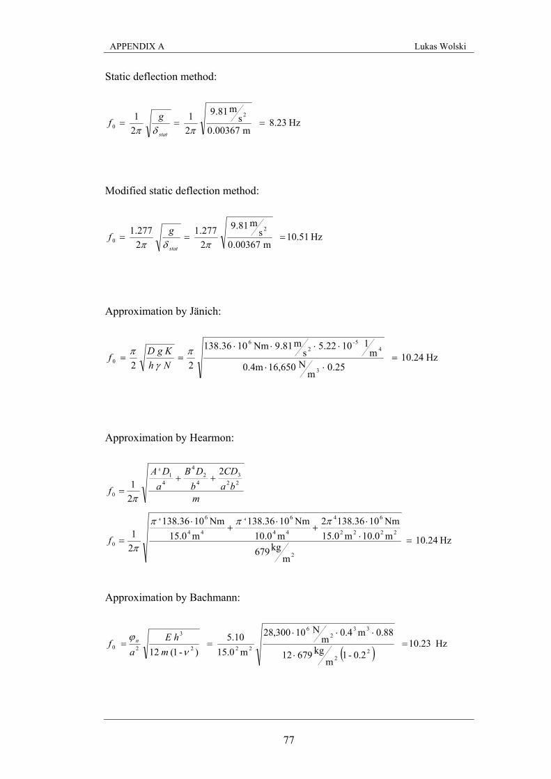
APPENDIX A Lukas Wolski
77
Static deflection method:
Hz 8.23 m 00367.0
sm 81.9
21
21
2
0 ===πδπ stat
gf
Modified static deflection method:
Hz 10.51 m 00367.0
sm 81.9
2277.1
2277.1
2
0 ===πδπ stat
gf
Approximation by Jänich:
Hz 10.24 25.0
mN 16,650 0.4m
m11022.5
sm81.9 Nm1036.138
2
2 3
45-
26
0 =⋅⋅
⋅⋅⋅⋅==π
γπ
Nhg KDf
Approximation by Hearmon:
Hz 10.24
mkg679
m0.10m0.15Nm1036.1382
m0.10Nm1036.138
m0.15Nm1036.138
21
2
21
2
2222
64
44
6
44
6
0
223
42
4
41
0
44
4
=⋅⋅
+⋅
+⋅
=
++=
πππ
π
π
f
mba
CDb
DBa
DA
f
Approximation by Bachmann:
( )Hz 10.23
0.2-1 m
kg679 12
0.88 m0.4 m
N10300,28
m15.05.10
)-1( 12
22
332
6
222
3
20 =⋅
⋅⋅⋅==
νϕ
mhE
af n
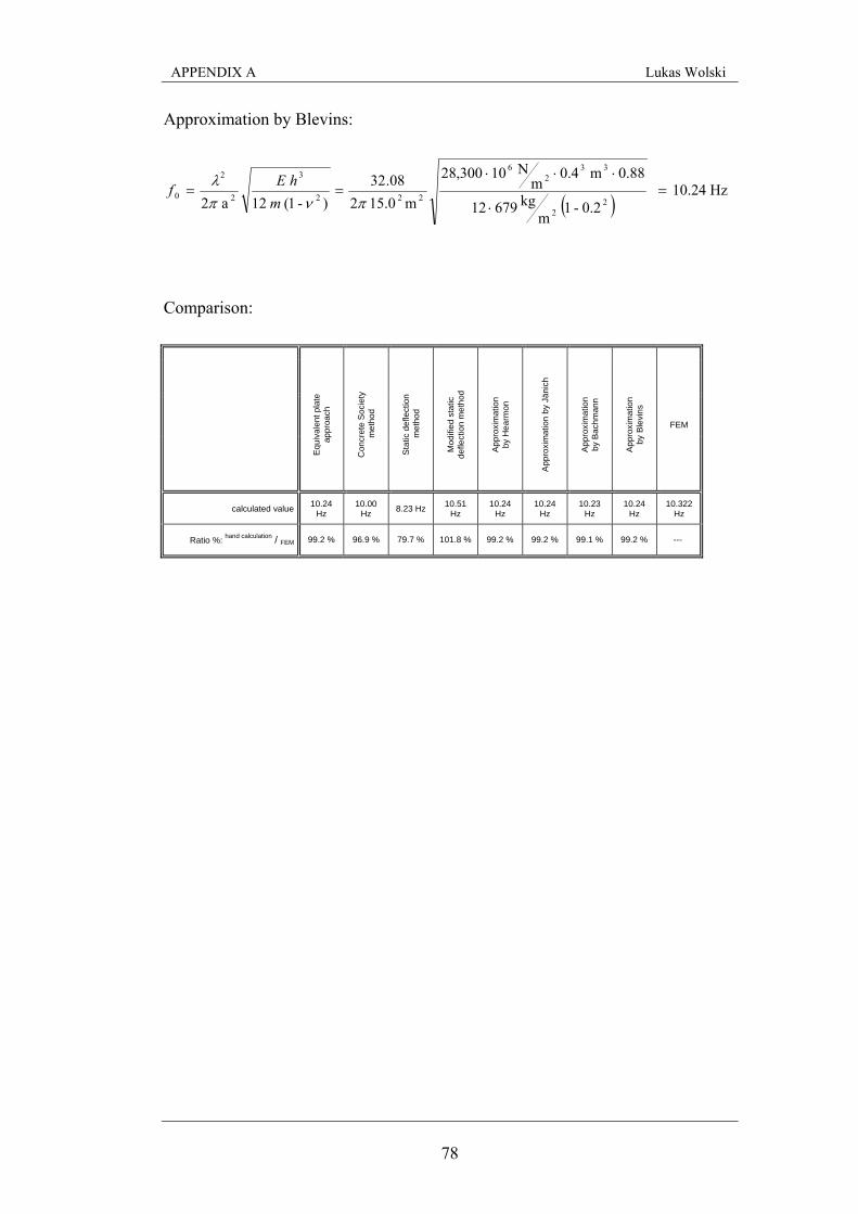
APPENDIX A Lukas Wolski
78
Approximation by Blevins:
( ) Hz 10.24
0.2-1 m
kg679 12
0.88 m 0.4 m
N10300,28
m15.0 208.32
)-1( 12
a 2 22
332
6
222
3
2
2
0 =⋅
⋅⋅⋅==
πνπλ
mhEf
Comparison:
Equ
ival
ent p
late
ap
proa
ch
Con
cret
e S
ocie
ty
met
hod
Sta
tic d
efle
ctio
n m
etho
d
Mod
ified
sta
tic
defle
ctio
n m
etho
d
App
roxi
mat
ion
by
Hea
rmon
App
roxi
mat
ion
by J
änic
h
App
roxi
mat
ion
by
Bac
hman
n
App
roxi
mat
ion
by
Ble
vins
FEM
calculated value 10.24 Hz
10.00 Hz 8.23 Hz 10.51
Hz 10.24
Hz 10.24
Hz 10.23
Hz 10.24
Hz 10.322
Hz
Ratio %: hand calculation / FEM 99.2 % 96.9 % 79.7 % 101.8 % 99.2 % 99.2 % 99.1 % 99.2 % ---
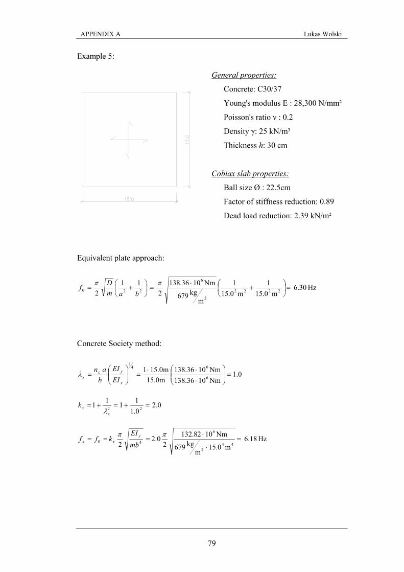
APPENDIX A Lukas Wolski
79
Example 5:
General properties:
Concrete: C30/37
Young's modulus E : 28,300 N/mm²
Poisson's ratio ν : 0.2
Density γ: 25 kN/m³
Thickness h: 30 cm
Cobiax slab properties:
Ball size Ø : 22.5cm
Factor of stiffness reduction: 0.89
Dead load reduction: 2.39 kN/m²
Equivalent plate approach:
Hz 6.30 m0.15
1m0.15
1
mkg 796
Nm1036.1382
11 2 2222
2
6
220 =⎟⎠⎞
⎜⎝⎛ +
⋅=⎟
⎠⎞
⎜⎝⎛ +=
ππbam
Df
Concrete Society method:
0.1Nm1036.381Nm1036.381
m0.15m0.151
6
641
=⎟⎟⎠
⎞⎜⎜⎝
⎛
⋅⋅⋅
=⎟⎟⎠
⎞⎜⎜⎝
⎛=
x
yxx EI
EIb
anλ
0.20.11111 22 =+=+=
xxk
λ
Hz 6.18 m0.15
mkg679
Nm1082.1322
2.0 2
44
2
6
40' =
⋅
⋅===
ππmbEI
kff yxx

APPENDIX A Lukas Wolski
80
Static deflection method:
Hz 5.05 m 00975.0
sm 81.9
21
21
2
0 ===πδπ stat
gf
Modified static deflection method:
Hz 6.44 m 75.009.0
sm 81.9
2277.1
2277.1
2
0 ===πδπ stat
gf
Approximation by Jänich:
Hz 6.30 25.0
mN 16,650 0.4m
m110975.1
sm81.9 Nm1036.138
2
2 3
45-
26
0 =⋅⋅
⋅⋅⋅⋅==π
γπ
Nhg KDf
Approximation by Hearmon:
Hz 6.30
mkg679
m0.15m0.15Nm1036.1382
m0.15Nm1036.138
m0.15Nm1036.138
21
2
21
2
2222
64
44
6
44
6
0
223
42
4
41
0
44
4
=⋅⋅
+⋅
+⋅
=
++=
πππ
π
π
f
mba
CDb
DBa
DA
f
Approximation by Bachmann:
( )Hz 6.29
0.2-1 m
kg679 12
0.88 m0.4 m
N10300,28
m15.03.14
)-1( 12
22
332
6
222
3
20 =⋅
⋅⋅⋅==
νϕ
mhE
af n
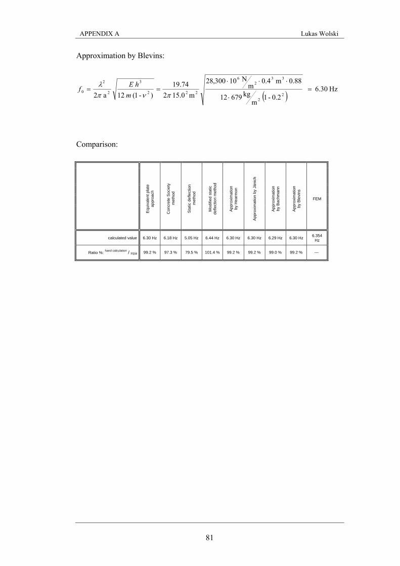
APPENDIX A Lukas Wolski
81
Approximation by Blevins:
( ) Hz 6.30
0.2-1 m
kg679 12
0.88 m 0.4 m
N10300,28
m15.0 274.19
)-1( 12
a 2 22
332
6
222
3
2
2
0 =⋅
⋅⋅⋅==
πνπλ
mhEf
Comparison:
Equ
ival
ent p
late
ap
proa
ch
Con
cret
e S
ocie
ty
met
hod
Sta
tic d
efle
ctio
n m
etho
d
Mod
ified
sta
tic
defle
ctio
n m
etho
d
App
roxi
mat
ion
by
Hea
rmon
App
roxi
mat
ion
by J
änic
h
App
roxi
mat
ion
by
Bac
hman
n
App
roxi
mat
ion
by
Ble
vins
FEM
calculated value 6.30 Hz 6.18 Hz 5.05 Hz 6.44 Hz 6.30 Hz 6.30 Hz 6.29 Hz 6.30 Hz 6.354 Hz
Ratio %: hand calculation / FEM 99.2 % 97.3 % 79.5 % 101.4 % 99.2 % 99.2 % 99.0 % 99.2 % ---
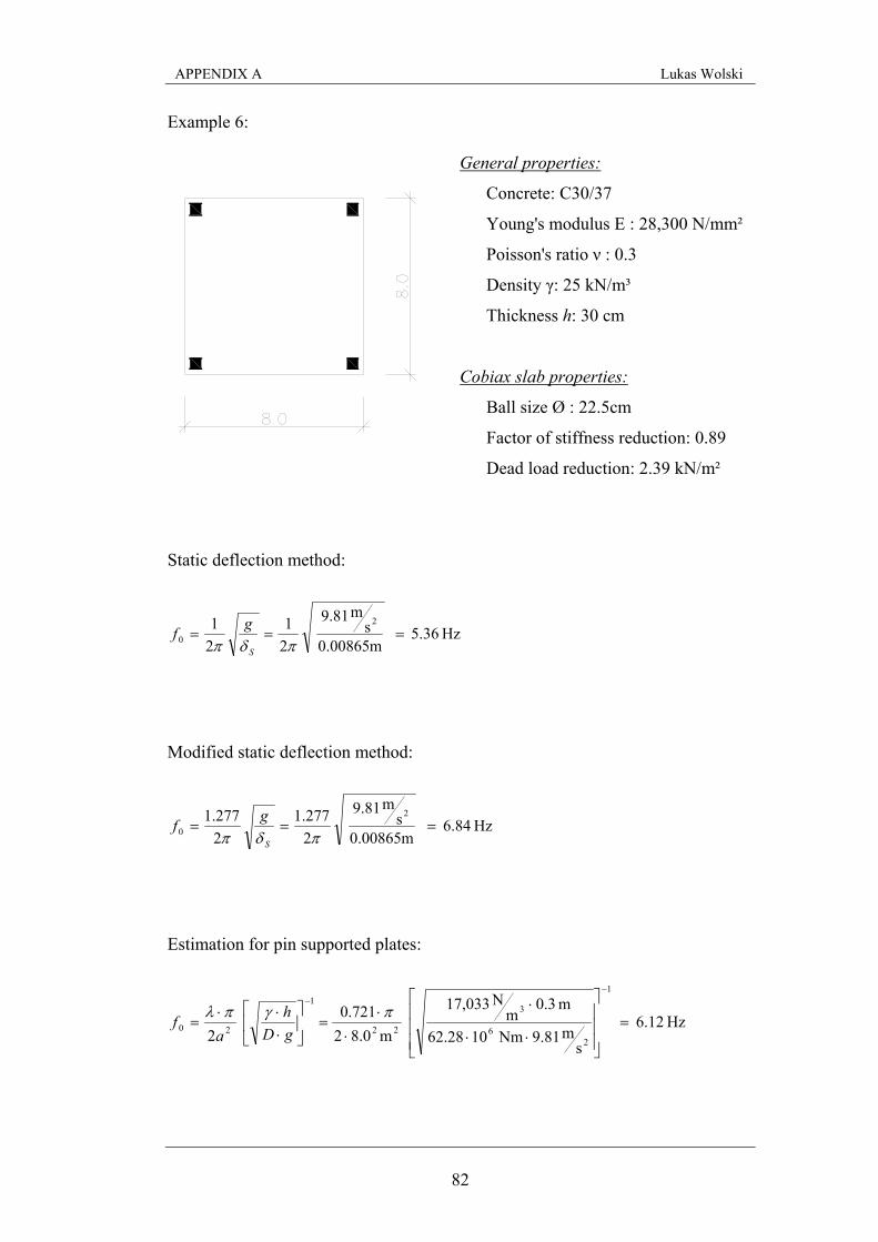
APPENDIX A Lukas Wolski
82
Example 6:
General properties:
Concrete: C30/37
Young's modulus E : 28,300 N/mm²
Poisson's ratio ν : 0.3
Density γ: 25 kN/m³
Thickness h: 30 cm
Cobiax slab properties:
Ball size Ø : 22.5cm
Factor of stiffness reduction: 0.89
Dead load reduction: 2.39 kN/m²
Static deflection method:
Hz 5.36 m00865.0
sm81.9
21
21 2
0 ===πδπ S
gf
Modified static deflection method:
Hz 6.84 m00865.0
sm81.9
2277.1
2277.1 2
0 ===πδπ S
gf
Estimation for pin supported plates:
Hz 6.12
sm 81.9Nm 1028.62
m 3.0m
N033,17
m0.82721.0
2
1
26
3
22
1
20 =⎥⎥⎥
⎦
⎤
⎢⎢⎢
⎣
⎡
⋅⋅
⋅
⋅⋅
=⎥⎦
⎤⎢⎣
⎡
⋅⋅⋅
=
−−
πγπλgDh
af
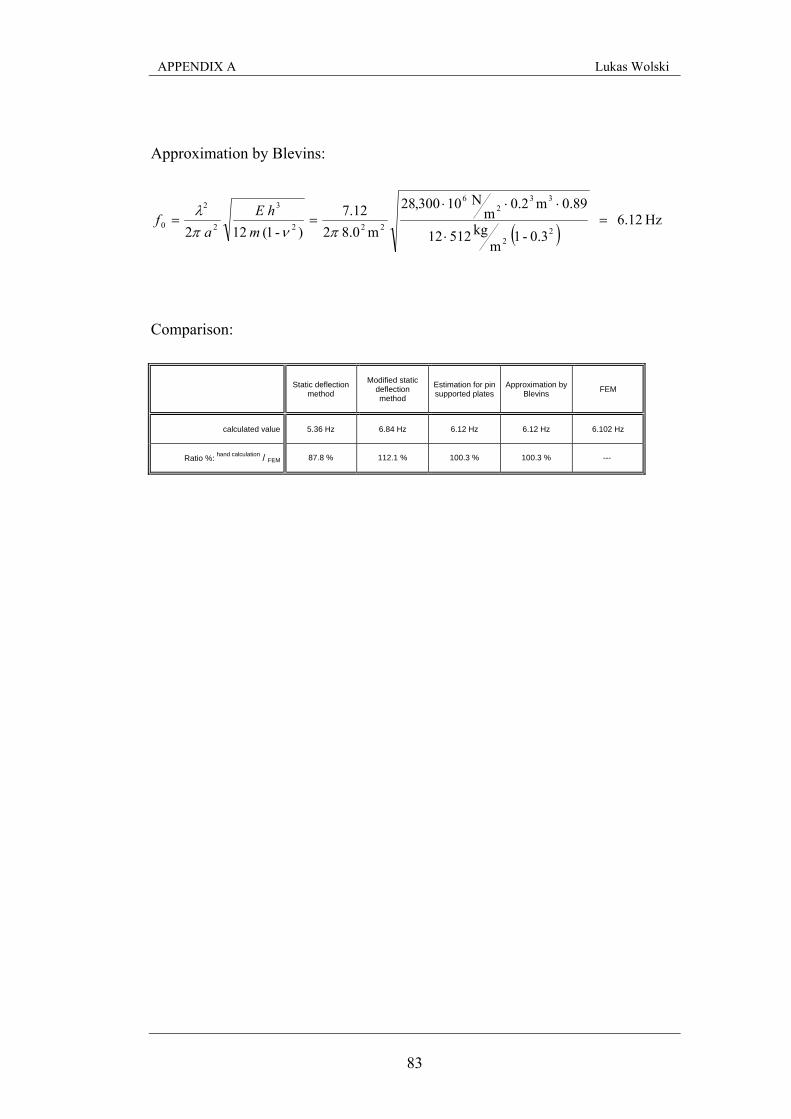
APPENDIX A Lukas Wolski
83
Approximation by Blevins:
( ) Hz 6.12
0.3-1 m
kg512 12
0.89 m0.2 m
N10300,28
m8.0 212.7
)-1( 12
2 22
332
6
222
3
2
2
0 =⋅
⋅⋅⋅==
πνπλ
mhE
af
Comparison:
Static deflection method
Modified static deflection method
Estimation for pin supported plates
Approximation by Blevins FEM
calculated value 5.36 Hz 6.84 Hz 6.12 Hz 6.12 Hz 6.102 Hz
Ratio %: hand calculation / FEM 87.8 % 112.1 % 100.3 % 100.3 % ---
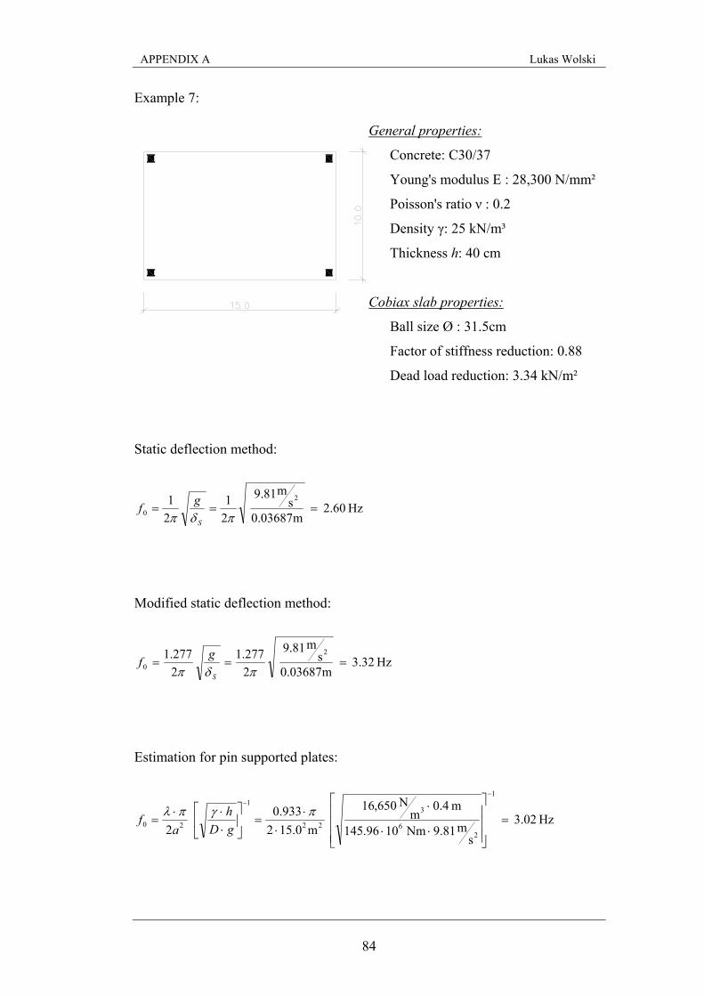
APPENDIX A Lukas Wolski
84
Example 7:
General properties:
Concrete: C30/37
Young's modulus E : 28,300 N/mm²
Poisson's ratio ν : 0.2
Density γ: 25 kN/m³
Thickness h: 40 cm
Cobiax slab properties:
Ball size Ø : 31.5cm
Factor of stiffness reduction: 0.88
Dead load reduction: 3.34 kN/m²
Static deflection method:
Hz 2.60 m03687.0
sm81.9
21
21 2
0 ===πδπ S
gf
Modified static deflection method:
Hz 3.32 m03687.0
sm81.9
2277.1
2277.1 2
0 ===πδπ S
gf
Estimation for pin supported plates:
Hz 3.02 s
m 81.9Nm 1096.145
m 4.0m
N650,16
m0.152933.0
2
1
26
3
22
1
20 =⎥⎥⎥
⎦
⎤
⎢⎢⎢
⎣
⎡
⋅⋅
⋅
⋅⋅
=⎥⎦
⎤⎢⎣
⎡
⋅⋅⋅
=
−−
πγπλgDh
af
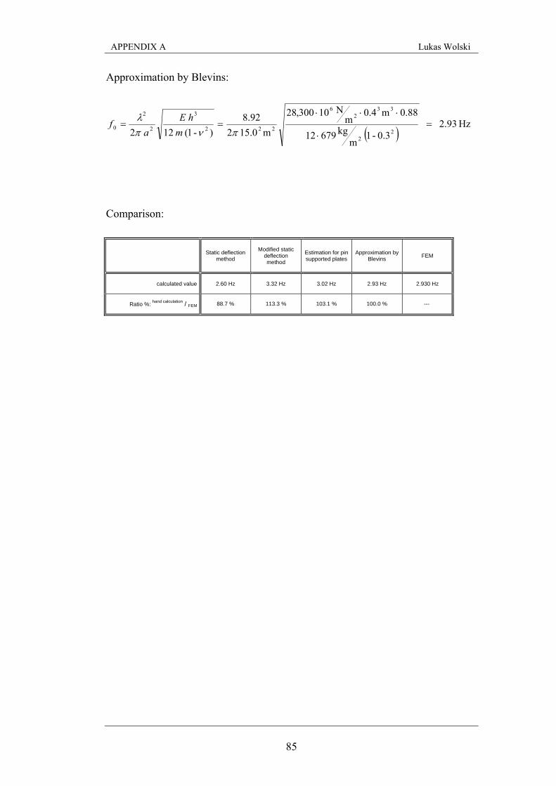
APPENDIX A Lukas Wolski
85
Approximation by Blevins:
( ) Hz 2.93
0.3-1 m
kg679 12
0.88 m0.4 m
N10300,28
m15.0 292.8
)-1( 12
2 22
332
6
222
3
2
2
0 =⋅
⋅⋅⋅==
πνπλ
mhE
af
Comparison:
Static deflection method
Modified static deflection method
Estimation for pin supported plates
Approximation by Blevins FEM
calculated value 2.60 Hz 3.32 Hz 3.02 Hz 2.93 Hz 2.930 Hz
Ratio %: hand calculation / FEM 88.7 % 113.3 % 103.1 % 100.0 % ---
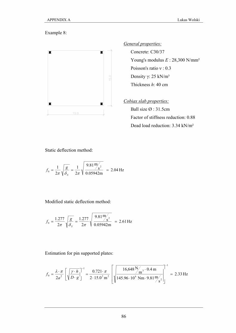
APPENDIX A Lukas Wolski
86
Example 8:
General properties:
Concrete: C30/37
Young's modulus E : 28,300 N/mm²
Poisson's ratio ν : 0.3
Density γ: 25 kN/m³
Thickness h: 40 cm
Cobiax slab properties:
Ball size Ø : 31.5cm
Factor of stiffness reduction: 0.88
Dead load reduction: 3.34 kN/m²
Static deflection method:
Hz 2.04 m05942.0
sm81.9
21
21 2
0 ===πδπ S
gf
Modified static deflection method:
Hz 2.61 m05942.0
sm81.9
2277.1
2277.1 2
0 ===πδπ S
gf
Estimation for pin supported plates:
Hz 2.33 s
m 81.9Nm 1096.145
m 4.0m
N648,16
m0.152721.0
2
1
26
3
22
1
20 =⎥⎥⎥
⎦
⎤
⎢⎢⎢
⎣
⎡
⋅⋅
⋅
⋅⋅
=⎥⎦
⎤⎢⎣
⎡
⋅⋅⋅
=
−−
πγπλgDh
af
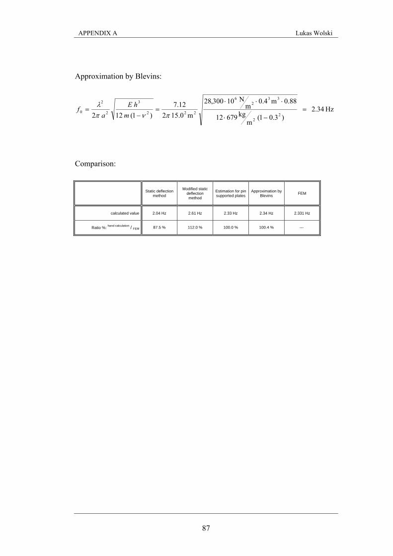
APPENDIX A Lukas Wolski
87
Approximation by Blevins:
Hz 2.34 )3.01(
mkg679 12
0.88 m0.4 m
N10300,28
m15.0 212.7
)1( 12
2 22
332
6
222
3
2
2
0 =−⋅
⋅⋅⋅=
−=
πνπλ
mhE
af
Comparison:
Static deflection method
Modified static deflection method
Estimation for pin supported plates
Approximation by Blevins FEM
calculated value 2.04 Hz 2.61 Hz 2.33 Hz 2.34 Hz 2.331 Hz
Ratio %: hand calculation / FEM 87.5 % 112.0 % 100.0 % 100.4 % ---
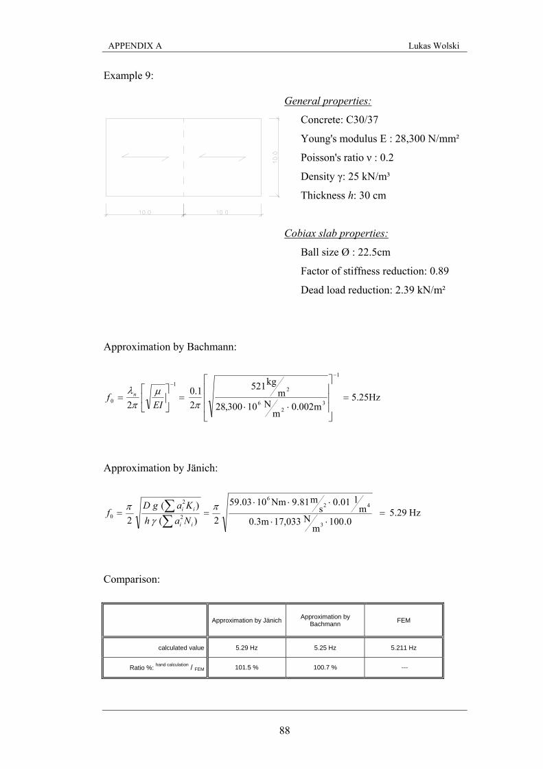
APPENDIX A Lukas Wolski
88
Example 9:
General properties:
Concrete: C30/37
Young's modulus E : 28,300 N/mm²
Poisson's ratio ν : 0.2
Density γ: 25 kN/m³
Thickness h: 30 cm
Cobiax slab properties:
Ball size Ø : 22.5cm
Factor of stiffness reduction: 0.89
Dead load reduction: 2.39 kN/m²
Approximation by Bachmann:
Hz25.5m002.0
mN10300,28
mkg521
2
1.0 2
1
32
6
21
0 =⎥⎥⎥
⎦
⎤
⎢⎢⎢
⎣
⎡
⋅⋅=⎥
⎦
⎤⎢⎣
⎡=
−
−
πμ
πλ
EIf n
Approximation by Jänich:
Hz 5.29 0.100
mN 17,033 0.3m
m101.0
sm81.9 Nm1003.59
2)( )(
2 3
426
2
2
0 =⋅⋅
⋅⋅⋅==
∑∑ π
γπ
ii
ii
NahKag D
f
Comparison:
Approximation by Jänich Approximation by Bachmann FEM
calculated value 5.29 Hz 5.25 Hz 5.211 Hz
Ratio %: hand calculation / FEM 101.5 % 100.7 % ---
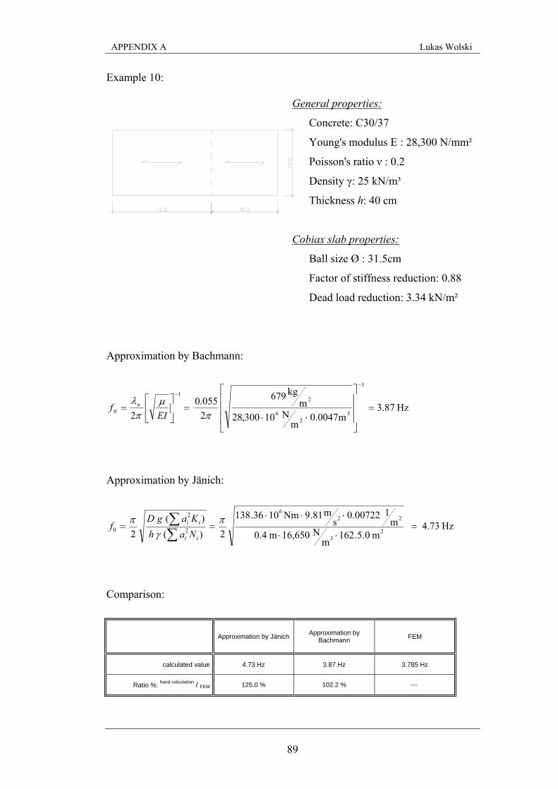
APPENDIX A Lukas Wolski
89
Example 10:
General properties:
Concrete: C30/37
Young's modulus E : 28,300 N/mm²
Poisson's ratio ν : 0.2
Density γ: 25 kN/m³
Thickness h: 40 cm
Cobiax slab properties:
Ball size Ø : 31.5cm
Factor of stiffness reduction: 0.88
Dead load reduction: 3.34 kN/m²
Approximation by Bachmann:
Hz 87.3m0047.0
mN10300,28
mkg679
2055.0
2
1
32
6
21
0 =⎥⎥⎥
⎦
⎤
⎢⎢⎢
⎣
⎡
⋅⋅=⎥
⎦
⎤⎢⎣
⎡=
−
−
πμ
πλ
EIf n
Approximation by Jänich:
Hz 4.73 m 0.5.162
mN 16,650 m 0.4
m100722.0
sm81.9 Nm1036.138
2)( )(
2 23
226
2
2
0 =⋅⋅
⋅⋅⋅==
∑∑ π
γπ
ii
ii
NahKag D
f
Comparison:
Approximation by Jänich Approximation by Bachmann FEM
calculated value 4.73 Hz 3.87 Hz 3.785 Hz
Ratio %: hand calculation / FEM 125.0 % 102.2 % ---
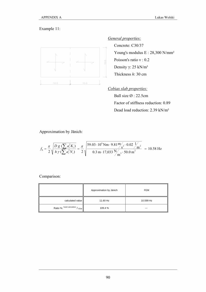
APPENDIX A Lukas Wolski
90
Example 11:
General properties:
Concrete: C30/37
Young's modulus E : 28,300 N/mm²
Poisson's ratio ν : 0.2
Density γ: 25 kN/m³
Thickness h: 30 cm
Cobiax slab properties:
Ball size Ø : 22.5cm
Factor of stiffness reduction: 0.89
Dead load reduction: 2.39 kN/m²
Approximation by Jänich:
Hz 10.58 m 0.50
mN 17,033 m 0.3
m102.0
sm81.9 Nm1003.59
2)( )(
2 23
226
2
2
0 =⋅⋅
⋅⋅⋅==
∑∑ π
γπ
ii
ii
NahKag D
f
Comparison:
Approximation by Jänich FEM
calculated value 11.60 Hz 10.599 Hz
Ratio %: hand calculation / FEM 109.4 % ---
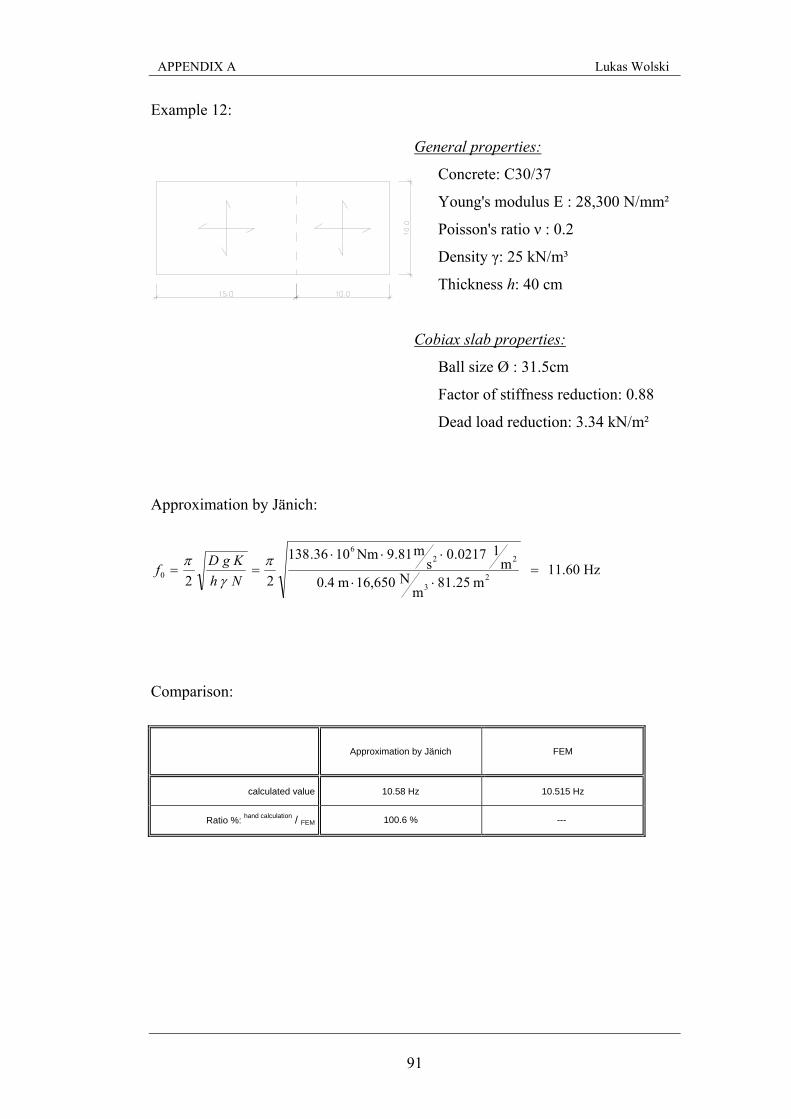
APPENDIX A Lukas Wolski
91
Example 12:
General properties:
Concrete: C30/37
Young's modulus E : 28,300 N/mm²
Poisson's ratio ν : 0.2
Density γ: 25 kN/m³
Thickness h: 40 cm
Cobiax slab properties:
Ball size Ø : 31.5cm
Factor of stiffness reduction: 0.88
Dead load reduction: 3.34 kN/m²
Approximation by Jänich:
Hz 11.60 m 25.81
mN 16,650 m 0.4
m10217.0
sm81.9 Nm1036.138
2
2 23
226
0 =⋅⋅
⋅⋅⋅==π
γπ
Nhg KDf
Comparison:
Approximation by Jänich FEM
calculated value 10.58 Hz 10.515 Hz
Ratio %: hand calculation / FEM 100.6 % ---
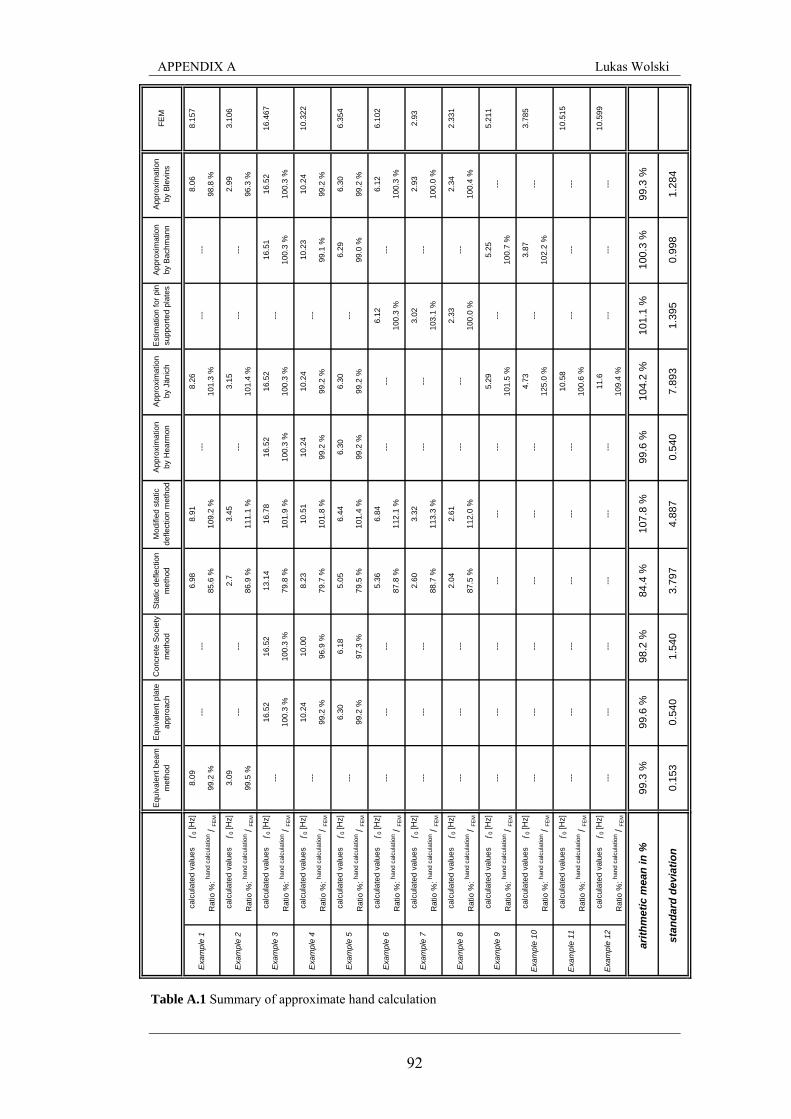
APPENDIX A Lukas Wolski
92
Table A.1 Summary of approximate hand calculation
calc
ulat
ed v
alue
s
f 0 [H
z]8.
096.
988.
918.
268.
068.
157
Rat
io %
: hand
cal
cula
tion /
FEM
99.2
%85
.6 %
109.
2 %
101.
3 %
98.8
%
calc
ulat
ed v
alue
s
f 0 [H
z]3.
092.
73.
453.
152.
993.
106
Rat
io %
: hand
cal
cula
tion /
FEM
99.5
%86
.9 %
111.
1 %
101.
4 %
96.3
%
calc
ulat
ed v
alue
s
f 0 [H
z]16
.52
16.5
213
.14
16.7
816
.52
16.5
216
.51
16.5
216
.467
Rat
io %
: hand
cal
cula
tion /
FEM
100.
3 %
100.
3 %
79.8
%10
1.9
%10
0.3
%10
0.3
%10
0.3
%10
0.3
%
calc
ulat
ed v
alue
s
f 0 [H
z]10
.24
10.0
08.
2310
.51
10.2
410
.24
10.2
310
.24
10.3
22
Rat
io %
: hand
cal
cula
tion /
FEM
99.2
%96
.9 %
79.7
%10
1.8
%99
.2 %
99.2
%99
.1 %
99.2
%
calc
ulat
ed v
alue
s
f 0 [H
z]6.
306.
185.
056.
446.
306.
306.
296.
306.
354
Rat
io %
: hand
cal
cula
tion /
FEM
99.2
%97
.3 %
79.5
%10
1.4
%99
.2 %
99.2
%99
.0 %
99.2
%
calc
ulat
ed v
alue
s
f 0 [H
z]5.
366.
846.
126.
126.
102
Rat
io %
: hand
cal
cula
tion /
FEM
87.8
%11
2.1
%10
0.3
%10
0.3
%
calc
ulat
ed v
alue
s
f 0 [H
z]2.
603.
323.
022.
932.
93
Rat
io %
: hand
cal
cula
tion /
FEM
88.7
%11
3.3
%10
3.1
%10
0.0
%
calc
ulat
ed v
alue
s
f 0 [H
z]2.
042.
612.
332.
342.
331
Rat
io %
: hand
cal
cula
tion /
FEM
87.5
%11
2.0
%10
0.0
%10
0.4
%
calc
ulat
ed v
alue
s
f 0 [H
z]5.
295.
255.
211
Rat
io %
: hand
cal
cula
tion /
FEM
101.
5 %
100.
7 %
calc
ulat
ed v
alue
s
f 0 [H
z]4.
733.
873.
785
Rat
io %
: hand
cal
cula
tion /
FEM
125.
0 %
102.
2 %
calc
ulat
ed v
alue
s
f 0 [H
z]10
.58
10.5
15
Rat
io %
: hand
cal
cula
tion /
FEM
100.
6 %
calc
ulat
ed v
alue
s
f 0 [H
z]11
.610
.599
Rat
io %
: hand
cal
cula
tion /
FEM
109.
4 %
99.3
%
0.15
30.
540
1.54
03.
797
4.88
70.
540
1.39
50.
998
1.28
4
107.
8 %
99.6
%10
1.1
%10
0.3
%10
4.2
%99
.6 %
98.2
%84
.4 %
Exa
mpl
e 5
Exa
mpl
e 6
Exa
mpl
e 7
Exa
mpl
e 8
Exa
mpl
e 1
---
99.3
%
---
---
---
---
---
---
---
Exa
mpl
e 2
Exa
mpl
e 3
Exa
mpl
e 4
Equ
ival
ent b
eam
m
etho
d
---
---
Equ
ival
ent p
late
ap
proa
chC
oncr
ete
Soc
iety
m
etho
dS
tatic
def
lect
ion
met
hod
App
roxi
mat
ion
by B
levi
nsFE
MM
odifi
ed s
tatic
de
flect
ion
met
hod
App
roxi
mat
ion
by H
earm
onE
stim
atio
n fo
r pin
su
ppor
ted
plat
esA
ppro
xim
atio
n by
Bac
hman
n A
ppro
xim
atio
n by
Jän
ich
Exa
mpl
e 9
Exa
mpl
e 10
Exa
mpl
e 11
Exa
mpl
e 12
7.89
3
arith
met
ic m
ean
in %
stan
dard
dev
iatio
n
---
---
---
---
---
---
---
---
---
---
---
---
---
---
---
---
---
---
---
---
---
---
---
---
---
---
---
---
---
---
---
---
---
---
---
---
---
---
---
---
---
---
---
---
---
---
---
---
---
---
---
---
---
---
---
---
---
---
APPENDIX B Lukas Wolski
93
APPENDIX B
(Calculated Values by FEM) Simply supported slab, one-way spanning ............................................................94
Simply supported slab, two-way spanning ...........................................................95
2 span slab, two-way spanning .............................................................................96
3 span slab, two-way spanning .............................................................................97
1x1 bay slab, supported by columns .....................................................................98
2x1 bay slab, supported by columns .....................................................................99
3x3 bay slab, supported by columns ...................................................................100
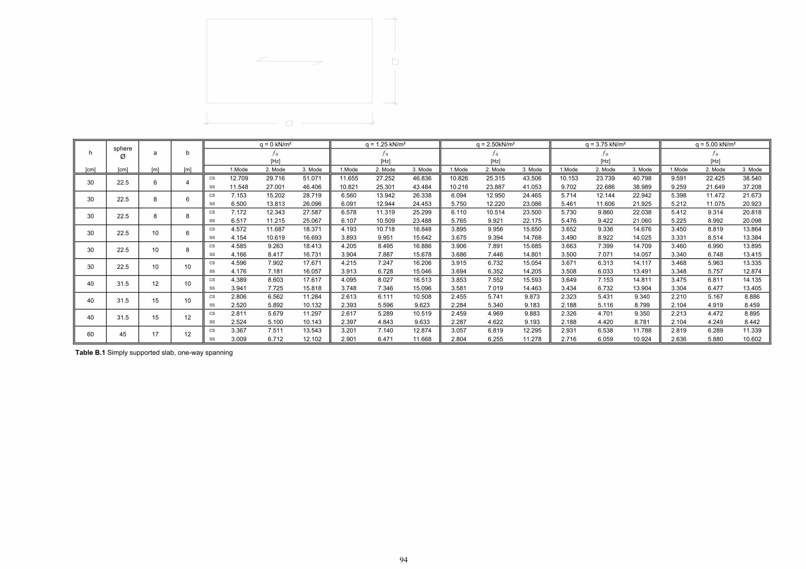
q = 0 kN/m² q = 1.25 kN/m² q = 2.50kN/m² q = 3.75 kN/m² q = 5.00 kN/m²f 0 f 0 f 0 f 0 f 0
[Hz] [Hz] [Hz] [Hz] [Hz][cm] [cm] [m] [m] 1.Mode 2. Mode 3. Mode 1.Mode 2. Mode 3. Mode 1.Mode 2. Mode 3. Mode 1.Mode 2. Mode 3. Mode 1.Mode 2. Mode 3. Mode
CS 12.709 29.716 51.071 11.655 27.252 46.836 10.826 25.315 43.506 10.153 23.739 40.798 9.591 22.425 38.540SS 11.548 27.001 46.406 10.821 25.301 43.484 10.216 23.887 41.053 9.702 22.686 38.989 9.259 21.649 37.208CS 7.153 15.202 28.719 6.560 13.942 26.338 6.094 12.950 24.465 5.714 12.144 22.942 5.398 11.472 21.673SS 6.500 13.813 26.096 6.091 12.944 24.453 5.750 12.220 23.086 5.461 11.606 21.925 5.212 11.075 20.923CS 7.172 12.343 27.587 6.578 11.319 25.299 6.110 10.514 23.500 5.730 9.860 22.038 5.412 9.314 20.818SS 6.517 11.215 25.067 6.107 10.509 23.488 5.765 9.921 22.175 5.476 9.422 21.060 5.225 8.992 20.098CS 4.572 11.687 18.371 4.193 10.718 16.848 3.895 9.956 15.650 3.652 9.336 14.676 3.450 8.819 13.864SS 4.154 10.619 16.693 3.893 9.951 15.642 3.675 9.394 14.768 3.490 8.922 14.025 3.331 8.514 13.384CS 4.585 9.263 18.413 4.205 8.495 16.886 3.906 7.891 15.685 3.663 7.399 14.709 3.460 6.990 13.895SS 4.166 8.417 16.731 3.904 7.887 15.678 3.686 7.446 14.801 3.500 7.071 14.057 3.340 6.748 13.415CS 4.596 7.902 17.671 4.215 7.247 16.206 3.915 6.732 15.054 3.671 6.313 14.117 3.468 5.963 13.335SS 4.176 7.181 16.057 3.913 6.728 15.046 3.694 6.352 14.205 3.508 6.033 13.491 3.348 5.757 12.874CS 4.389 8.603 17.617 4.095 8.027 16.513 3.853 7.552 15.593 3.649 7.153 14.811 3.475 6.811 14.135SS 3.941 7.725 15.818 3.748 7.346 15.096 3.581 7.019 14.463 3.434 6.732 13.904 3.304 6.477 13.405CS 2.806 6.562 11.284 2.613 6.111 10.508 2.455 5.741 9.873 2.323 5.431 9.340 2.210 5.167 8.886SS 2.520 5.892 10.132 2.393 5.596 9.623 2.284 5.340 9.183 2.188 5.116 8.799 2.104 4.919 8.459CS 2.811 5.679 11.297 2.617 5.289 10.519 2.459 4.969 9.883 2.326 4.701 9.350 2.213 4.472 8.895SS 2.524 5.100 10.143 2.397 4.843 9.633 2.287 4.622 9.193 2.188 4.420 8.781 2.104 4.249 8.442CS 3.367 7.511 13.543 3.201 7.140 12.874 3.057 6.819 12.295 2.931 6.538 11.788 2.819 6.289 11.339SS 3.009 6.712 12.102 2.901 6.471 11.668 2.804 6.255 11.278 2.716 6.059 10.924 2.636 5.880 10.602
Table B.1 Simply supported slab, one-way spanning
asphere
Øh b
15 12
60 45 17 12
12 10
31.5 15 10
40
40
40
31.5
31.5
30 22.5 10 10
30 22.5 10 8
30 22.5 10 6
30 22.5 8 8
30 22.5 8 6
30 22.5 6 4
94
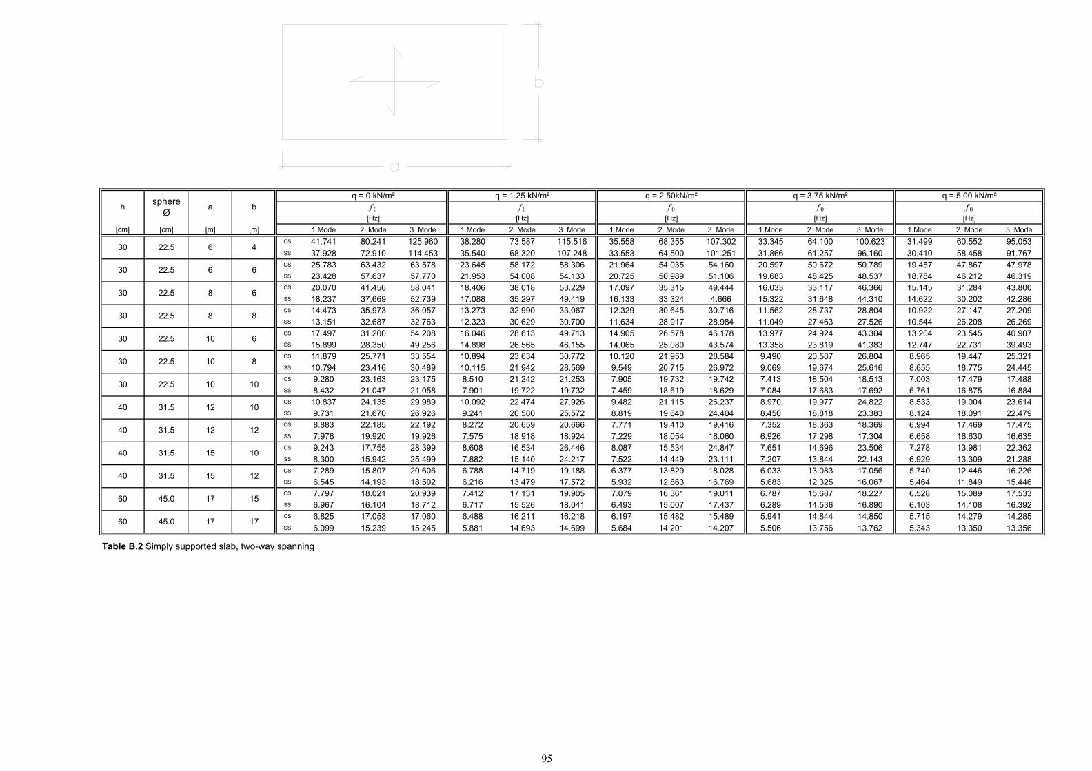
q = 0 kN/m² q = 1.25 kN/m² q = 2.50kN/m² q = 3.75 kN/m² q = 5.00 kN/m²f 0 f 0 f 0 f 0 f 0
[Hz] [Hz] [Hz] [Hz] [Hz][cm] [cm] [m] [m] 1.Mode 2. Mode 3. Mode 1.Mode 2. Mode 3. Mode 1.Mode 2. Mode 3. Mode 1.Mode 2. Mode 3. Mode 1.Mode 2. Mode 3. Mode
CS 41.741 80.241 125.960 38.280 73.587 115.516 35.558 68.355 107.302 33.345 64.100 100.623 31.499 60.552 95.053SS 37.928 72.910 114.453 35.540 68.320 107.248 33.553 64.500 101.251 31.866 61.257 96.160 30.410 58.458 91.767CS 25.783 63.432 63.578 23.645 58.172 58.306 21.964 54.035 54.160 20.597 50.672 50.789 19.457 47.867 47.978SS 23.428 57.637 57.770 21.953 54.008 54.133 20.725 50.989 51.106 19.683 48.425 48.537 18.784 46.212 46.319CS 20.070 41.456 58.041 18.406 38.018 53.229 17.097 35.315 49.444 16.033 33.117 46.366 15.145 31.284 43.800SS 18.237 37.669 52.739 17.088 35.297 49.419 16.133 33.324 4.666 15.322 31.648 44.310 14.622 30.202 42.286CS 14.473 35.973 36.057 13.273 32.990 33.067 12.329 30.645 30.716 11.562 28.737 28.804 10.922 27.147 27.209SS 13.151 32.687 32.763 12.323 30.629 30.700 11.634 28.917 28.984 11.049 27.463 27.526 10.544 26.208 26.269CS 17.497 31.200 54.208 16.046 28.613 49.713 14.905 26.578 46.178 13.977 24.924 43.304 13.204 23.545 40.907SS 15.899 28.350 49.256 14.898 26.565 46.155 14.065 25.080 43.574 13.358 23.819 41.383 12.747 22.731 39.493CS 11.879 25.771 33.554 10.894 23.634 30.772 10.120 21.953 28.584 9.490 20.587 26.804 8.965 19.447 25.321SS 10.794 23.416 30.489 10.115 21.942 28.569 9.549 20.715 26.972 9.069 19.674 25.616 8.655 18.775 24.445CS 9.280 23.163 23.175 8.510 21.242 21.253 7.905 19.732 19.742 7.413 18.504 18.513 7.003 17.479 17.488SS 8.432 21.047 21.058 7.901 19.722 19.732 7.459 18.619 18.629 7.084 17.683 17.692 6.761 16.875 16.884CS 10.837 24.135 29.989 10.092 22.474 27.926 9.482 21.115 26.237 8.970 19.977 24.822 8.533 19.004 23.614SS 9.731 21.670 26.926 9.241 20.580 25.572 8.819 19.640 24.404 8.450 18.818 23.383 8.124 18.091 22.479CS 8.883 22.185 22.192 8.272 20.659 20.666 7.771 19.410 19.416 7.352 18.363 18.369 6.994 17.469 17.475SS 7.976 19.920 19.926 7.575 18.918 18.924 7.229 18.054 18.060 6.926 17.298 17.304 6.658 16.630 16.635CS 9.243 17.755 28.399 8.608 16.534 26.446 8.087 15.534 24.847 7.651 14.696 23.506 7.278 13.981 22.362SS 8.300 15.942 25.499 7.882 15.140 24.217 7.522 14.449 23.111 7.207 13.844 22.143 6.929 13.309 21.288CS 7.289 15.807 20.606 6.788 14.719 19.188 6.377 13.829 18.028 6.033 13.083 17.056 5.740 12.446 16.226SS 6.545 14.193 18.502 6.216 13.479 17.572 5.932 12.863 16.769 5.683 12.325 16.067 5.464 11.849 15.446CS 7.797 18.021 20.939 7.412 17.131 19.905 7.079 16.361 19.011 6.787 15.687 18.227 6.528 15.089 17.533SS 6.967 16.104 18.712 6.717 15.526 18.041 6.493 15.007 17.437 6.289 14.536 16.890 6.103 14.108 16.392CS 6.825 17.053 17.060 6.488 16.211 16.218 6.197 15.482 15.489 5.941 14.844 14.850 5.715 14.279 14.285SS 6.099 15.239 15.245 5.881 14.693 14.699 5.684 14.201 14.207 5.506 13.756 13.762 5.343 13.350 13.356
Table B.2 Simply supported slab, two-way spanning
60 45.0 17 17
60 45.0 17 15
40 31.5 15 12
40 31.5 15 10
40 31.5 12 12
40 31.5 12 10
30 22.5 10 10
30 22.5 10 8
30 22.5 10 6
30 22.5 8 8
30 22.5 8 6
30 22.5 6 6
30 22.5 6 4
sphere Øh a b
95
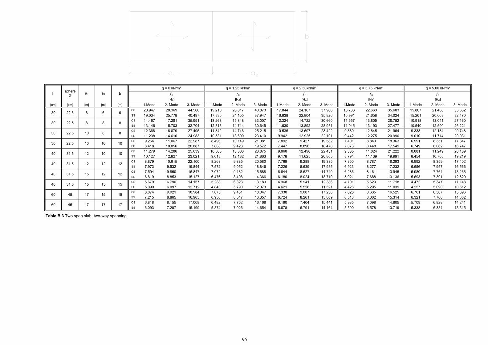
q = 0 kN/m² q = 1.25 kN/m² q = 2.50kN/m² q = 3.75 kN/m² q = 5.00 kN/m²f 0 f 0 f 0 f 0 f 0
[Hz] [Hz] [Hz] [Hz] [Hz][cm] [cm] [m] [m] [m] 1.Mode 2. Mode 3. Mode 1.Mode 2. Mode 3. Mode 1.Mode 2. Mode 3. Mode 1.Mode 2. Mode 3. Mode 1.Mode 2. Mode 3. Mode
CS 20.947 28.369 44.568 19.210 26.017 40.873 17.844 24.167 37.966 16.733 22.663 35.603 15.807 21.408 33.632SS 19.034 25.778 40.497 17.835 24.155 37.947 16.838 22.804 35.826 15.991 21.658 34.024 15.261 20.668 32.470CS 14.467 17.281 35.991 13.268 15.848 33.007 12.324 14.722 30.660 11.557 13.805 28.752 10.918 13.041 27.160SS 13.146 15.703 32.704 12.318 14.714 30.645 11.630 13.892 28.931 11.045 13.193 27.477 10.540 12.590 26.221CS 12.368 16.079 27.495 11.342 14.746 25.215 10.536 13.697 23.422 9.880 12.845 21.964 9.333 12.134 20.748SS 11.238 14.610 24.983 10.531 13.690 23.410 9.942 12.925 22.101 9.442 12.275 20.990 9.010 11.714 20.031CS 9.264 11.067 22.987 8.496 10.149 21.081 7.892 9.427 19.582 7.401 8.840 18.363 6.991 8.351 17.347SS 8.418 10.056 20.887 7.888 9.423 19.572 7.447 8.896 18.478 7.073 8.448 17.549 6.749 8.062 16.747CS 11.279 14.286 25.639 10.503 13.303 23.875 9.868 12.498 22.431 9.335 11.824 21.222 8.881 11.249 20.189SS 10.127 12.827 23.021 9.618 12.182 21.863 9.178 11.625 20.865 8.794 11.139 19.991 8.454 10.708 19.219CS 8.879 10.615 22.100 8.268 9.885 20.580 7.769 9.288 19.335 7.350 8.787 18.293 6.992 8.359 17.402SS 7.973 9.532 19.844 7.572 9.052 18.846 7.226 8.639 17.985 6.923 8.277 17.232 6.656 7.957 16.566CS 7.594 9.860 16.847 7.072 9.182 15.688 6.644 8.627 14.740 6.286 8.161 13.945 5.980 7.764 13.266SS 6.819 8.853 15.127 6.476 8.408 14.366 6.180 8.024 13.710 5.921 7.688 13.136 5.693 7.391 12.629CS 5.679 6.790 14.157 5.288 6.323 13.183 4.968 5.941 12.386 4.701 5.620 11.718 4.472 5.347 11.148SS 5.099 6.097 12.712 4.843 5.790 12.073 4.621 5.526 11.521 4.428 5.295 11.039 4.257 5.090 10.612CS 8.074 9.921 18.984 7.675 9.431 18.047 7.330 9.007 17.236 7.028 8.635 16.525 6.761 8.307 15.896SS 7.215 8.865 16.965 6.956 8.547 16.357 6.724 8.261 15.809 6.513 8.002 15.314 6.321 7.766 14.862CS 6.818 8.155 17.008 6.482 7.752 16.168 6.190 7.404 15.441 5.935 7.098 14.805 5.709 6.828 14.241SS 6.093 7.287 15.199 5.874 7.026 14.654 5.678 6.791 14.164 5.500 6.578 13.719 5.338 6.384 13.315
Table B.3 Two span slab, two-way spanning
bh sphere Ø
a1 a2
15
60 45 17 17 17
60 45 17 15
12
40 31.5 15 15 15
40 31.5 15 12
10
40 31.5 12 12 12
40 31.5 12 10
8
30 22.5 10 10 10
30 22.5 10 8
6
30 22.5 8 8 8
30 22.5 8 6
96
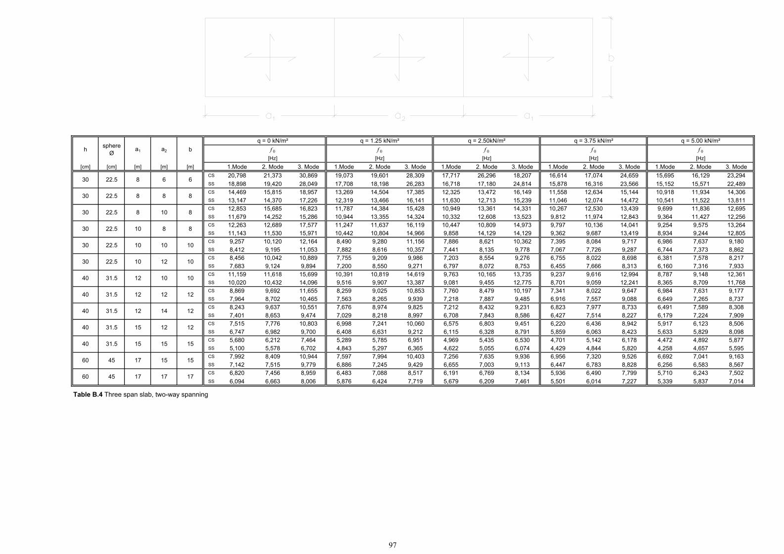
q = 0 kN/m² q = 1.25 kN/m² q = 2.50kN/m² q = 3.75 kN/m² q = 5.00 kN/m²f 0 f 0 f 0 f 0 f 0
[Hz] [Hz] [Hz] [Hz] [Hz][cm] [cm] [m] [m] [m] 1.Mode 2. Mode 3. Mode 1.Mode 2. Mode 3. Mode 1.Mode 2. Mode 3. Mode 1.Mode 2. Mode 3. Mode 1.Mode 2. Mode 3. Mode
CS 20,798 21,373 30,869 19,073 19,601 28,309 17,717 26,296 18,207 16,614 17,074 24,659 15,695 16,129 23,294SS 18,898 19,420 28,049 17,708 18,198 26,283 16,718 17,180 24,814 15,878 16,316 23,566 15,152 15,571 22,489CS 14,469 15,815 18,957 13,269 14,504 17,385 12,325 13,472 16,149 11,558 12,634 15,144 10,918 11,934 14,306SS 13,147 14,370 17,226 12,319 13,466 16,141 11,630 12,713 15,239 11,046 12,074 14,472 10,541 11,522 13,811CS 12,853 15,685 16,823 11,787 14,384 15,428 10,949 13,361 14,331 10,267 12,530 13,439 9,699 11,836 12,695SS 11,679 14,252 15,286 10,944 13,355 14,324 10,332 12,608 13,523 9,812 11,974 12,843 9,364 11,427 12,256CS 12,263 12,689 17,577 11,247 11,637 16,119 10,447 10,809 14,973 9,797 10,136 14,041 9,254 9,575 13,264SS 11,143 11,530 15,971 10,442 10,804 14,966 9,858 14,129 14,129 9,362 9,687 13,419 8,934 9,244 12,805CS 9,257 10,120 12,164 8,490 9,280 11,156 7,886 8,621 10,362 7,395 8,084 9,717 6,986 7,637 9,180SS 8,412 9,195 11,053 7,882 8,616 10,357 7,441 8,135 9,778 7,067 7,726 9,287 6,744 7,373 8,862CS 8,456 10,042 10,889 7,755 9,209 9,986 7,203 8,554 9,276 6,755 8,022 8,698 6,381 7,578 8,217SS 7,683 9,124 9,894 7,200 8,550 9,271 6,797 8,072 8,753 6,455 7,666 8,313 6,160 7,316 7,933CS 11,159 11,618 15,699 10,391 10,819 14,619 9,763 10,165 13,735 9,237 9,616 12,994 8,787 9,148 12,361SS 10,020 10,432 14,096 9,516 9,907 13,387 9,081 9,455 12,775 8,701 9,059 12,241 8,365 8,709 11,768CS 8,869 9,692 11,655 8,259 9,025 10,853 7,760 8,479 10,197 7,341 8,022 9,647 6,984 7,631 9,177SS 7,964 8,702 10,465 7,563 8,265 9,939 7,218 7,887 9,485 6,916 7,557 9,088 6,649 7,265 8,737CS 8,243 9,637 10,551 7,676 8,974 9,825 7,212 8,432 9,231 6,823 7,977 8,733 6,491 7,589 8,308SS 7,401 8,653 9,474 7,029 8,218 8,997 6,708 7,843 8,586 6,427 7,514 8,227 6,179 7,224 7,909CS 7,515 7,776 10,803 6,998 7,241 10,060 6,575 6,803 9,451 6,220 6,436 8,942 5,917 6,123 8,506SS 6,747 6,982 9,700 6,408 6,631 9,212 6,115 6,328 8,791 5,859 6,063 8,423 5,633 5,829 8,098CS 5,680 6,212 7,464 5,289 5,785 6,951 4,969 5,435 6,530 4,701 5,142 6,178 4,472 4,892 5,877SS 5,100 5,578 6,702 4,843 5,297 6,365 4,622 5,055 6,074 4,429 4,844 5,820 4,258 4,657 5,595CS 7,992 8,409 10,944 7,597 7,994 10,403 7,256 7,635 9,936 6,956 7,320 9,526 6,692 7,041 9,163SS 7,142 7,515 9,779 6,886 7,245 9,429 6,655 7,003 9,113 6,447 6,783 8,828 6,256 6,583 8,567CS 6,820 7,456 8,959 6,483 7,088 8,517 6,191 6,769 8,134 5,936 6,490 7,799 5,710 6,243 7,502SS 6,094 6,663 8,006 5,876 6,424 7,719 5,679 6,209 7,461 5,501 6,014 7,227 5,339 5,837 7,014
Table B.4 Three span slab, two-way spanning
17
h sphere Ø
a1 a2 b
60 45 17 17
15
60 45 17 15 15
40 31.5 15 15
12
40 31.5 15 12 12
40 31.5 12 14
10
40 31.5 12 12 12
40 31.5 12 10
10
30 22.5 10 12 10
30 22.5 10 10
8
30 22.5 10 8 8
30 22.5 8 10
6
30 22.5 8 8 8
30 22.5 8 6
97
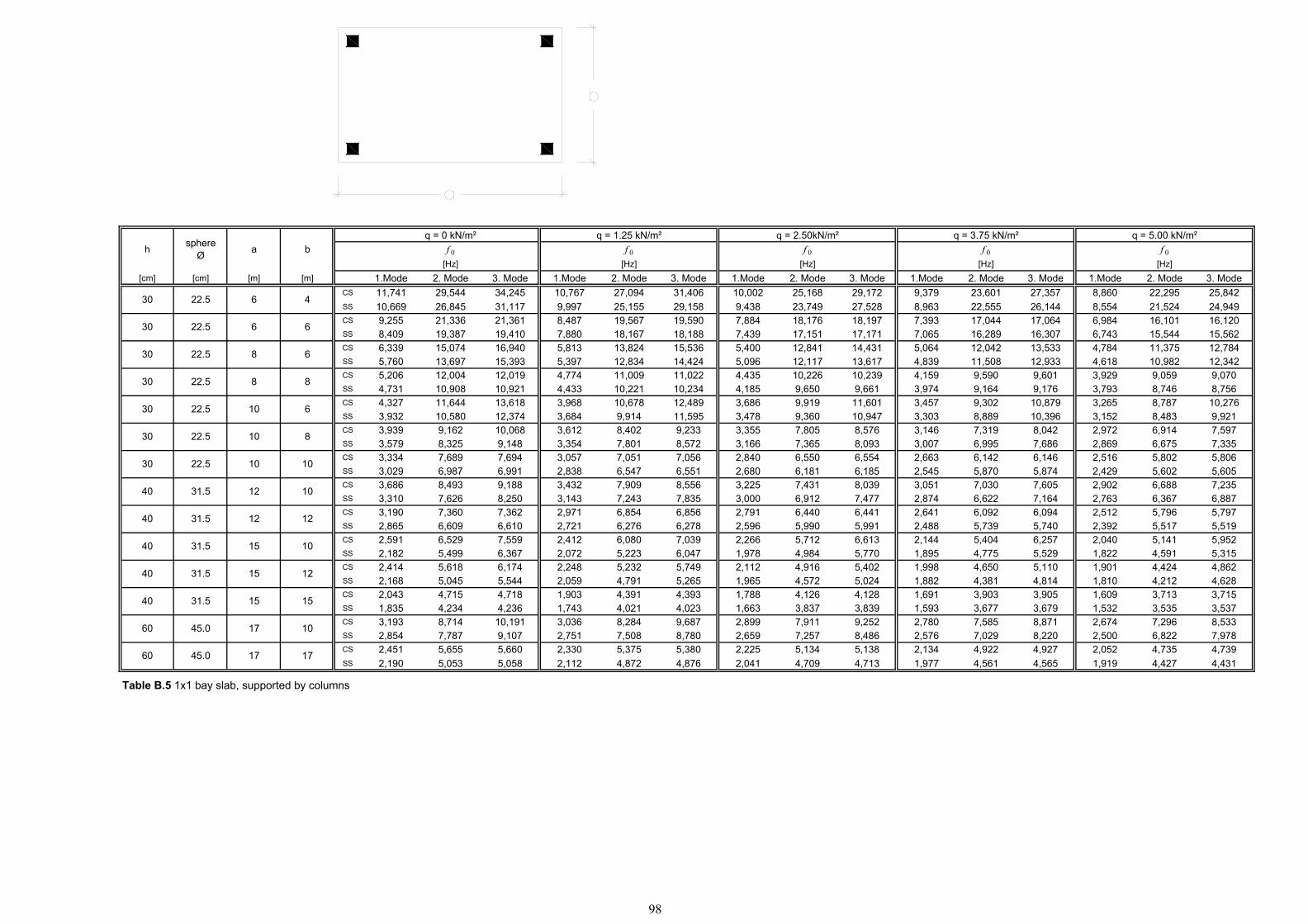
q = 0 kN/m² q = 1.25 kN/m² q = 2.50kN/m² q = 3.75 kN/m² q = 5.00 kN/m²f 0 f 0 f 0 f 0 f 0
[Hz] [Hz] [Hz] [Hz] [Hz][cm] [cm] [m] [m] 1.Mode 2. Mode 3. Mode 1.Mode 2. Mode 3. Mode 1.Mode 2. Mode 3. Mode 1.Mode 2. Mode 3. Mode 1.Mode 2. Mode 3. Mode
CS 11,741 29,544 34,245 10,767 27,094 31,406 10,002 25,168 29,172 9,379 23,601 27,357 8,860 22,295 25,842SS 10,669 26,845 31,117 9,997 25,155 29,158 9,438 23,749 27,528 8,963 22,555 26,144 8,554 21,524 24,949CS 9,255 21,336 21,361 8,487 19,567 19,590 7,884 18,176 18,197 7,393 17,044 17,064 6,984 16,101 16,120SS 8,409 19,387 19,410 7,880 18,167 18,188 7,439 17,151 17,171 7,065 16,289 16,307 6,743 15,544 15,562CS 6,339 15,074 16,940 5,813 13,824 15,536 5,400 12,841 14,431 5,064 12,042 13,533 4,784 11,375 12,784SS 5,760 13,697 15,393 5,397 12,834 14,424 5,096 12,117 13,617 4,839 11,508 12,933 4,618 10,982 12,342CS 5,206 12,004 12,019 4,774 11,009 11,022 4,435 10,226 10,239 4,159 9,590 9,601 3,929 9,059 9,070SS 4,731 10,908 10,921 4,433 10,221 10,234 4,185 9,650 9,661 3,974 9,164 9,176 3,793 8,746 8,756CS 4,327 11,644 13,618 3,968 10,678 12,489 3,686 9,919 11,601 3,457 9,302 10,879 3,265 8,787 10,276SS 3,932 10,580 12,374 3,684 9,914 11,595 3,478 9,360 10,947 3,303 8,889 10,396 3,152 8,483 9,921CS 3,939 9,162 10,068 3,612 8,402 9,233 3,355 7,805 8,576 3,146 7,319 8,042 2,972 6,914 7,597SS 3,579 8,325 9,148 3,354 7,801 8,572 3,166 7,365 8,093 3,007 6,995 7,686 2,869 6,675 7,335CS 3,334 7,689 7,694 3,057 7,051 7,056 2,840 6,550 6,554 2,663 6,142 6,146 2,516 5,802 5,806SS 3,029 6,987 6,991 2,838 6,547 6,551 2,680 6,181 6,185 2,545 5,870 5,874 2,429 5,602 5,605CS 3,686 8,493 9,188 3,432 7,909 8,556 3,225 7,431 8,039 3,051 7,030 7,605 2,902 6,688 7,235SS 3,310 7,626 8,250 3,143 7,243 7,835 3,000 6,912 7,477 2,874 6,622 7,164 2,763 6,367 6,887CS 3,190 7,360 7,362 2,971 6,854 6,856 2,791 6,440 6,441 2,641 6,092 6,094 2,512 5,796 5,797SS 2,865 6,609 6,610 2,721 6,276 6,278 2,596 5,990 5,991 2,488 5,739 5,740 2,392 5,517 5,519CS 2,591 6,529 7,559 2,412 6,080 7,039 2,266 5,712 6,613 2,144 5,404 6,257 2,040 5,141 5,952SS 2,182 5,499 6,367 2,072 5,223 6,047 1,978 4,984 5,770 1,895 4,775 5,529 1,822 4,591 5,315CS 2,414 5,618 6,174 2,248 5,232 5,749 2,112 4,916 5,402 1,998 4,650 5,110 1,901 4,424 4,862SS 2,168 5,045 5,544 2,059 4,791 5,265 1,965 4,572 5,024 1,882 4,381 4,814 1,810 4,212 4,628CS 2,043 4,715 4,718 1,903 4,391 4,393 1,788 4,126 4,128 1,691 3,903 3,905 1,609 3,713 3,715SS 1,835 4,234 4,236 1,743 4,021 4,023 1,663 3,837 3,839 1,593 3,677 3,679 1,532 3,535 3,537CS 3,193 8,714 10,191 3,036 8,284 9,687 2,899 7,911 9,252 2,780 7,585 8,871 2,674 7,296 8,533SS 2,854 7,787 9,107 2,751 7,508 8,780 2,659 7,257 8,486 2,576 7,029 8,220 2,500 6,822 7,978CS 2,451 5,655 5,660 2,330 5,375 5,380 2,225 5,134 5,138 2,134 4,922 4,927 2,052 4,735 4,739SS 2,190 5,053 5,058 2,112 4,872 4,876 2,041 4,709 4,713 1,977 4,561 4,565 1,919 4,427 4,431
Table B.5 1x1 bay slab, supported by columns
60 45.0 17 17
60 45.0 17 10
40 31.5 15 15
40 31.5 15 12
40 31.5 15 10
40 31.5 12 12
40 31.5 12 10
30 22.5 10 10
30 22.5 10 8
30 22.5 10 6
30 22.5 8 8
30 22.5 8 6
30 22.5 6 6
30 22.5 6 4
h sphere Ø a b
98
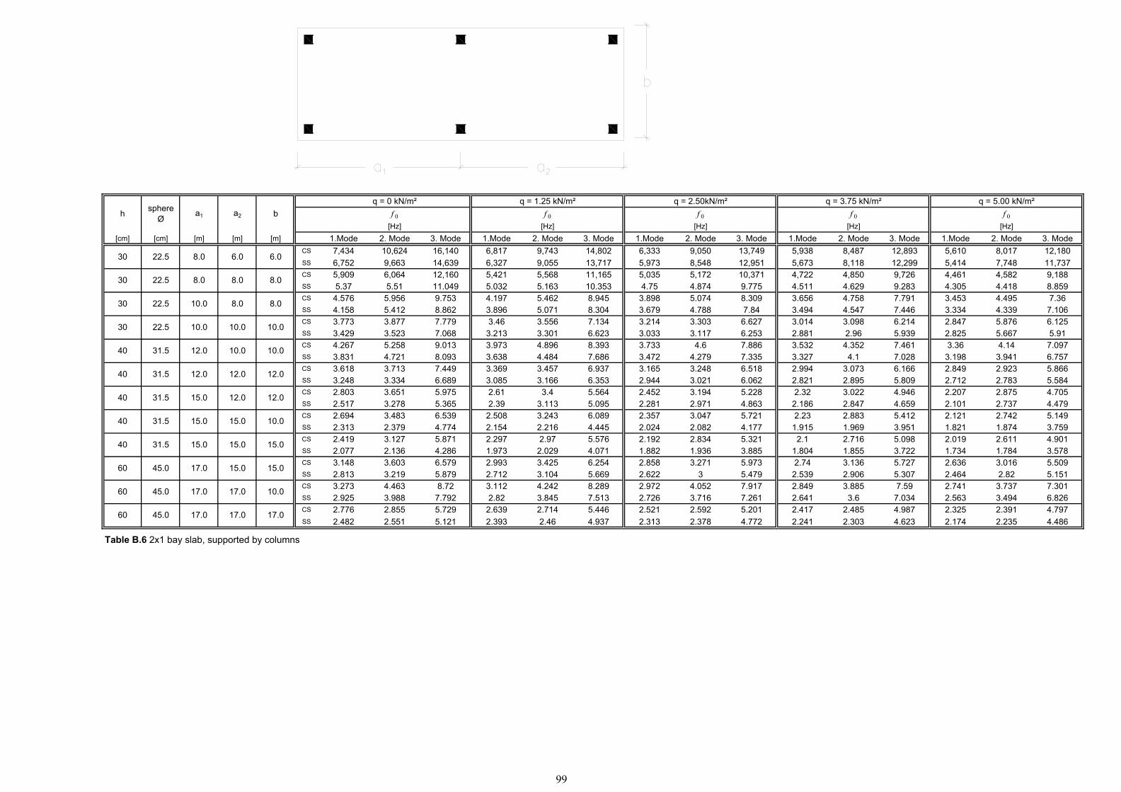
q = 0 kN/m² q = 1.25 kN/m² q = 2.50kN/m² q = 3.75 kN/m² q = 5.00 kN/m²f 0 f 0 f 0 f 0 f 0
[Hz] [Hz] [Hz] [Hz] [Hz][cm] [cm] [m] [m] [m] 1.Mode 2. Mode 3. Mode 1.Mode 2. Mode 3. Mode 1.Mode 2. Mode 3. Mode 1.Mode 2. Mode 3. Mode 1.Mode 2. Mode 3. Mode
CS 7,434 10,624 16,140 6,817 9,743 14,802 6,333 9,050 13,749 5,938 8,487 12,893 5,610 8,017 12,180SS 6,752 9,663 14,639 6,327 9,055 13,717 5,973 8,548 12,951 5,673 8,118 12,299 5,414 7,748 11,737CS 5,909 6,064 12,160 5,421 5,568 11,165 5,035 5,172 10,371 4,722 4,850 9,726 4,461 4,582 9,188SS 5.37 5.51 11.049 5.032 5.163 10.353 4.75 4.874 9.775 4.511 4.629 9.283 4.305 4.418 8.859CS 4.576 5.956 9.753 4.197 5.462 8.945 3.898 5.074 8.309 3.656 4.758 7.791 3.453 4.495 7.36SS 4.158 5.412 8.862 3.896 5.071 8.304 3.679 4.788 7.84 3.494 4.547 7.446 3.334 4.339 7.106CS 3.773 3.877 7.779 3.46 3.556 7.134 3.214 3.303 6.627 3.014 3.098 6.214 2.847 5.876 6.125SS 3.429 3.523 7.068 3.213 3.301 6.623 3.033 3.117 6.253 2.881 2.96 5.939 2.825 5.667 5.91CS 4.267 5.258 9.013 3.973 4.896 8.393 3.733 4.6 7.886 3.532 4.352 7.461 3.36 4.14 7.097SS 3.831 4.721 8.093 3.638 4.484 7.686 3.472 4.279 7.335 3.327 4.1 7.028 3.198 3.941 6.757CS 3.618 3.713 7.449 3.369 3.457 6.937 3.165 3.248 6.518 2.994 3.073 6.166 2.849 2.923 5.866SS 3.248 3.334 6.689 3.085 3.166 6.353 2.944 3.021 6.062 2.821 2.895 5.809 2.712 2.783 5.584CS 2.803 3.651 5.975 2.61 3.4 5.564 2.452 3.194 5.228 2.32 3.022 4.946 2.207 2.875 4.705SS 2.517 3.278 5.365 2.39 3.113 5.095 2.281 2.971 4.863 2.186 2.847 4.659 2.101 2.737 4.479CS 2.694 3.483 6.539 2.508 3.243 6.089 2.357 3.047 5.721 2.23 2.883 5.412 2.121 2.742 5.149SS 2.313 2.379 4.774 2.154 2.216 4.445 2.024 2.082 4.177 1.915 1.969 3.951 1.821 1.874 3.759CS 2.419 3.127 5.871 2.297 2.97 5.576 2.192 2.834 5.321 2.1 2.716 5.098 2.019 2.611 4.901SS 2.077 2.136 4.286 1.973 2.029 4.071 1.882 1.936 3.885 1.804 1.855 3.722 1.734 1.784 3.578CS 3.148 3.603 6.579 2.993 3.425 6.254 2.858 3.271 5.973 2.74 3.136 5.727 2.636 3.016 5.509SS 2.813 3.219 5.879 2.712 3.104 5.669 2.622 3 5.479 2.539 2.906 5.307 2.464 2.82 5.151CS 3.273 4.463 8.72 3.112 4.242 8.289 2.972 4.052 7.917 2.849 3.885 7.59 2.741 3.737 7.301SS 2.925 3.988 7.792 2.82 3.845 7.513 2.726 3.716 7.261 2.641 3.6 7.034 2.563 3.494 6.826CS 2.776 2.855 5.729 2.639 2.714 5.446 2.521 2.592 5.201 2.417 2.485 4.987 2.325 2.391 4.797SS 2.482 2.551 5.121 2.393 2.46 4.937 2.313 2.378 4.772 2.241 2.303 4.623 2.174 2.235 4.486
Table B.6 2x1 bay slab, supported by columns
17.060 45.0 17.0 17.0
15.0
60 45.0 17.0 17.0 10.0
60 45.0 17.0 15.0
10.0
40 31.5 15.0 15.0 15.0
40 31.5 15.0 15.0
12.0
40 31.5 15.0 12.0 12.0
40 31.5 12.0 12.0
10.0
40 31.5 12.0 10.0 10.0
30 22.5 10.0 10.0
8.0
30 22.5 10.0 8.0 8.0
30 22.5 8.0 8.0
b
30 22.5 8.0 6.0 6.0
h sphere Ø
a1 a2
99
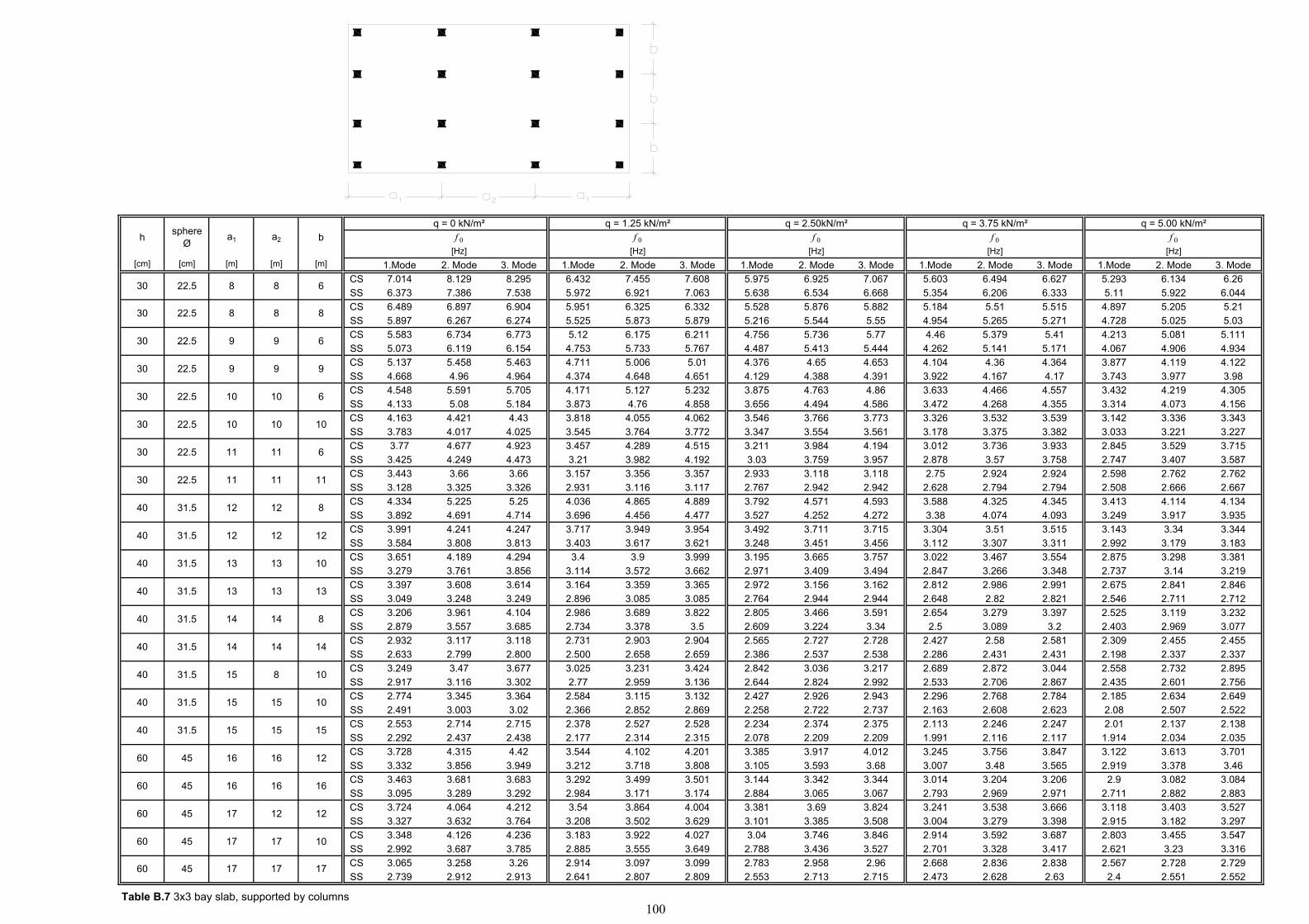
q = 0 kN/m² q = 1.25 kN/m² q = 2.50kN/m² q = 3.75 kN/m² q = 5.00 kN/m²f 0 f 0 f 0 f 0 f 0
[Hz] [Hz] [Hz] [Hz] [Hz][cm] [cm] [m] [m] [m] 1.Mode 2. Mode 3. Mode 1.Mode 2. Mode 3. Mode 1.Mode 2. Mode 3. Mode 1.Mode 2. Mode 3. Mode 1.Mode 2. Mode 3. Mode
CS 7.014 8.129 8.295 6.432 7.455 7.608 5.975 6.925 7.067 5.603 6.494 6.627 5.293 6.134 6.26SS 6.373 7.386 7.538 5.972 6.921 7.063 5.638 6.534 6.668 5.354 6.206 6.333 5.11 5.922 6.044CS 6.489 6.897 6.904 5.951 6.325 6.332 5.528 5.876 5.882 5.184 5.51 5.515 4.897 5.205 5.21SS 5.897 6.267 6.274 5.525 5.873 5.879 5.216 5.544 5.55 4.954 5.265 5.271 4.728 5.025 5.03CS 5.583 6.734 6.773 5.12 6.175 6.211 4.756 5.736 5.77 4.46 5.379 5.41 4.213 5.081 5.111SS 5.073 6.119 6.154 4.753 5.733 5.767 4.487 5.413 5.444 4.262 5.141 5.171 4.067 4.906 4.934CS 5.137 5.458 5.463 4.711 5.006 5.01 4.376 4.65 4.653 4.104 4.36 4.364 3.877 4.119 4.122SS 4.668 4.96 4.964 4.374 4.648 4.651 4.129 4.388 4.391 3.922 4.167 4.17 3.743 3.977 3.98CS 4.548 5.591 5.705 4.171 5.127 5.232 3.875 4.763 4.86 3.633 4.466 4.557 3.432 4.219 4.305SS 4.133 5.08 5.184 3.873 4.76 4.858 3.656 4.494 4.586 3.472 4.268 4.355 3.314 4.073 4.156CS 4.163 4.421 4.43 3.818 4.055 4.062 3.546 3.766 3.773 3.326 3.532 3.539 3.142 3.336 3.343SS 3.783 4.017 4.025 3.545 3.764 3.772 3.347 3.554 3.561 3.178 3.375 3.382 3.033 3.221 3.227CS 3.77 4.677 4.923 3.457 4.289 4.515 3.211 3.984 4.194 3.012 3.736 3.933 2.845 3.529 3.715SS 3.425 4.249 4.473 3.21 3.982 4.192 3.03 3.759 3.957 2.878 3.57 3.758 2.747 3.407 3.587CS 3.443 3.66 3.66 3.157 3.356 3.357 2.933 3.118 3.118 2.75 2.924 2.924 2.598 2.762 2.762SS 3.128 3.325 3.326 2.931 3.116 3.117 2.767 2.942 2.942 2.628 2.794 2.794 2.508 2.666 2.667CS 4.334 5.225 5.25 4.036 4.865 4.889 3.792 4.571 4.593 3.588 4.325 4.345 3.413 4.114 4.134SS 3.892 4.691 4.714 3.696 4.456 4.477 3.527 4.252 4.272 3.38 4.074 4.093 3.249 3.917 3.935CS 3.991 4.241 4.247 3.717 3.949 3.954 3.492 3.711 3.715 3.304 3.51 3.515 3.143 3.34 3.344SS 3.584 3.808 3.813 3.403 3.617 3.621 3.248 3.451 3.456 3.112 3.307 3.311 2.992 3.179 3.183CS 3.651 4.189 4.294 3.4 3.9 3.999 3.195 3.665 3.757 3.022 3.467 3.554 2.875 3.298 3.381SS 3.279 3.761 3.856 3.114 3.572 3.662 2.971 3.409 3.494 2.847 3.266 3.348 2.737 3.14 3.219CS 3.397 3.608 3.614 3.164 3.359 3.365 2.972 3.156 3.162 2.812 2.986 2.991 2.675 2.841 2.846SS 3.049 3.248 3.249 2.896 3.085 3.085 2.764 2.944 2.944 2.648 2.82 2.821 2.546 2.711 2.712CS 3.206 3.961 4.104 2.986 3.689 3.822 2.805 3.466 3.591 2.654 3.279 3.397 2.525 3.119 3.232SS 2.879 3.557 3.685 2.734 3.378 3.5 2.609 3.224 3.34 2.5 3.089 3.2 2.403 2.969 3.077CS 2.932 3.117 3.118 2.731 2.903 2.904 2.565 2.727 2.728 2.427 2.58 2.581 2.309 2.455 2.455SS 2.633 2.799 2.800 2.500 2.658 2.659 2.386 2.537 2.538 2.286 2.431 2.431 2.198 2.337 2.337CS 3.249 3.47 3.677 3.025 3.231 3.424 2.842 3.036 3.217 2.689 2.872 3.044 2.558 2.732 2.895SS 2.917 3.116 3.302 2.77 2.959 3.136 2.644 2.824 2.992 2.533 2.706 2.867 2.435 2.601 2.756CS 2.774 3.345 3.364 2.584 3.115 3.132 2.427 2.926 2.943 2.296 2.768 2.784 2.185 2.634 2.649SS 2.491 3.003 3.02 2.366 2.852 2.869 2.258 2.722 2.737 2.163 2.608 2.623 2.08 2.507 2.522CS 2.553 2.714 2.715 2.378 2.527 2.528 2.234 2.374 2.375 2.113 2.246 2.247 2.01 2.137 2.138SS 2.292 2.437 2.438 2.177 2.314 2.315 2.078 2.209 2.209 1.991 2.116 2.117 1.914 2.034 2.035CS 3.728 4.315 4.42 3.544 4.102 4.201 3.385 3.917 4.012 3.245 3.756 3.847 3.122 3.613 3.701SS 3.332 3.856 3.949 3.212 3.718 3.808 3.105 3.593 3.68 3.007 3.48 3.565 2.919 3.378 3.46CS 3.463 3.681 3.683 3.292 3.499 3.501 3.144 3.342 3.344 3.014 3.204 3.206 2.9 3.082 3.084SS 3.095 3.289 3.292 2.984 3.171 3.174 2.884 3.065 3.067 2.793 2.969 2.971 2.711 2.882 2.883CS 3.724 4.064 4.212 3.54 3.864 4.004 3.381 3.69 3.824 3.241 3.538 3.666 3.118 3.403 3.527SS 3.327 3.632 3.764 3.208 3.502 3.629 3.101 3.385 3.508 3.004 3.279 3.398 2.915 3.182 3.297CS 3.348 4.126 4.236 3.183 3.922 4.027 3.04 3.746 3.846 2.914 3.592 3.687 2.803 3.455 3.547SS 2.992 3.687 3.785 2.885 3.555 3.649 2.788 3.436 3.527 2.701 3.328 3.417 2.621 3.23 3.316CS 3.065 3.258 3.26 2.914 3.097 3.099 2.783 2.958 2.96 2.668 2.836 2.838 2.567 2.728 2.729SS 2.739 2.912 2.913 2.641 2.807 2.809 2.553 2.713 2.715 2.473 2.628 2.63 2.4 2.551 2.552
Table B.7 3x3 bay slab, supported by columns
60
60
60
60
60
45
45
45
45
40
40
40
40
40
40
40
40
30
30
30
40
30
30
30
30
31.5
31.5
31.5
45
31.5
31.5
31.5
31.5
17
22.5
22.5
22.5
22.5
22.5
22.5
22.5
31.5
31.5
12
16
12
10
14
10
10
15
12
10
13
8
6
8
6
9
6
10
6
11
8
17
16
16
12
17
14
8
15
15
12
13
13
14
17
8
8
9
9
10
10
11
11
12
16
16
17
17
14
15
15
15
12
13
13
14
10
11
11
12
8
9
9
10
b
30 22.5 8
h sphere Ø
a1 a2
100
APPENDIX C Lukas Wolski
101
APPENDIX C
(Cobiax Information) Existing Cobiax projects .....................................................................................102
Summary of stiffness reduction ..........................................................................103
Design considerations .........................................................................................104
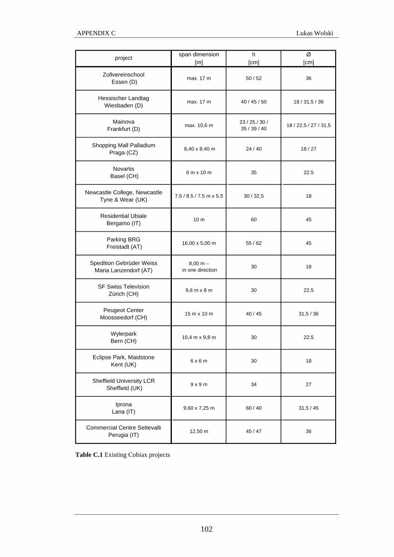
APPENDIX C Lukas Wolski
102
span dimension h Ø[m] [cm] [cm]
project
max. 17 m 50 / 52 36
Hessischer LandtagWiesbaden (D)
max. 17 m 40 / 45 / 50 18 / 31,5 / 36
MainovaFrankfurt (D)
max. 10,6 m 23 / 25 / 30 / 35 / 39 / 40 18 / 22,5 / 27 / 31,5
Shopping Mall PalladiumPraga (CZ)
8,40 x 8,40 m 24 / 40 18 / 27
Novartis Basel (CH)
6 m x 10 m 35 22.5
7.5 / 8.5 / 7.5 m x 5.5 30 / 32,5 18
10 mResidential UbialeBergamo (IT)
60 45
Parking BRG Freistadt (AT)
16,00 x 5,00 m 55 / 62 45
8,00 m – in one direction 30 18
SF Swiss TelevisionZürich (CH)
9,6 m x 8 m 30 22.5
Peugeot CenterMoosseedorf (CH)
15 m x 10 m 40 / 45 31,5 / 36
Wylerpark Bern (CH)
10,4 m x 9,8 m 30 22.5
Eclipse Park, Maidstone Kent (UK)
6 x 6 m 30 18
27
IpronaLana (IT)
9,60 x 7,25 m 60 / 40 31,5 / 45
12,50 m 45 / 47 36
Zollvereinschool Essen (D)
Newcastle College, Newcastle Tyne & Wear (UK)
Spedition Gebrüder Weiss Maria Lanzendorf (AT)
Sheffield University LCR Sheffield (UK)
Commercial Centre SettevalliPerugia (IT)
9 x 9 m 34
Table C.1 Existing Cobiax projects
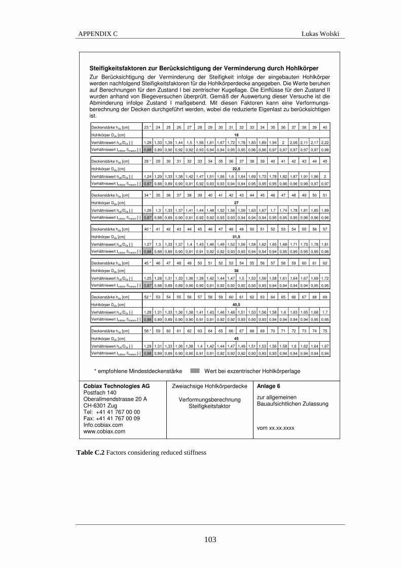
APPENDIX C Lukas Wolski
103
Table C.2 Factors considering reduced stiffness
Cobiax Technologies AGPostfach 140Oberallmendstrasse 20 ACH-6301 ZugTel: +41 41 767 00 00Fax: +41 41 767 00 09Info.cobiax.comwww.cobiax.com
Zweiachsige Hohlkörperdecke
VerformungsberechnungSteifigkeitsfaktor
Anlage 6
zur allgemeinenBauaufsichtlichen Zulassung
vom xx.xx.xxxx
Steifigkeitsfaktoren zur Berücksichtigung der Verminderung durch HohlkörperZur Berücksichtigung der Verminderung der Steifigkeit infolge der eingebauten Hohlkörperwerden nachfolgend Steifigkeitsfaktoren für die Hohlkörperdecke angegeben. Die Werte beruhenauf Berechnungen für den Zustand I bei zentrischer Kugellage. Die Einflüsse für den Zustand IIwurden anhand von Biegeversuchen überprüft. Gemäß der Auswertung dieser Versuche ist dieAbminderung infolge Zustand I maßgebend. Mit diesen Faktoren kann eine Verformungs-berechnung der Decken durchgeführt werden, wobei die reduzierte Eigenlast zu berücksichtigenist.
* empfohlene Mindestdeckenstärke Wert bei exzentrischer Hohlkörperlage
Deckenstärke hcb [cm] 23 * 24 25 26 27 28 29 30 31 32 33 34 35 36 37 38 39 40
Hohlkörper Dcb [cm]
Verhältniswert hcb/Dcb [-] 1,28 1,33 1,39 1,44 1,5 1,56 1,61 1,67 1,72 1,78 1,83 1,89 1,94 2 2,06 2,11 2,17 2,22
Verhältniswert Ιcobiax /Ιmassiv [-] 0,88 0,89 0,90 0,92 0,92 0,93 0,94 0,94 0,95 0,95 0,96 0,96 0,97 0,97 0,97 0,97 0,97 0,98
Deckenstärke hcb [cm] 28 * 29 30 31 32 33 34 35 36 37 38 39 40 41 42 43 44 45
Hohlkörper Dcb [cm]
Verhältniswert hcb/Dcb [-] 1,24 1,29 1,33 1,38 1,42 1,47 1,51 1,56 1,6 1,64 1,69 1,73 1,78 1,82 1,87 1,91 1,96 2
Verhältniswert Ιcobiax /Ιmassiv [-] 0,87 0,88 0,89 0,90 0,91 0,92 0,93 0,93 0,94 0,94 0,95 0,95 0,95 0,96 0,96 0,96 0,97 0,97
Deckenstärke hcb [cm] 34 * 35 36 37 38 39 40 41 42 43 44 45 46 47 48 49 50 51
Hohlkörper Dcb [cm]
Verhältniswert hcb/Dcb [-] 1,26 1,3 1,33 1,37 1,41 1,44 1,48 1,52 1,56 1,59 1,63 1,67 1,7 1,74 1,78 1,81 1,85 1,89
Verhältniswert Ιcobiax /Ιmassiv [-] 0,87 0,88 0,89 0,90 0,91 0,92 0,92 0,93 0,93 0,94 0,94 0,94 0,95 0,95 0,95 0,96 0,96 0,96
Deckenstärke hcb [cm] 40 * 41 42 43 44 45 46 47 48 49 50 51 52 53 54 55 56 57
Hohlkörper Dcb [cm]
Verhältniswert hcb/Dcb [-] 1,27 1,3 1,33 1,37 1,4 1,43 1,46 1,49 1,52 1,56 1,59 1,62 1,65 1,68 1,71 1,75 1,78 1,81
Verhältniswert Ιcobiax /Ιmassiv [-] 0,88 0,88 0,89 0,90 0,91 0,91 0,92 0,92 0,93 0,93 0,94 0,94 0,94 0,95 0,95 0,95 0,95 0,96
Deckenstärke hcb [cm] 45 * 46 47 48 49 50 51 52 53 54 55 56 57 58 59 60 61 62
Hohlkörper Dcb [cm]
Verhältniswert hcb/Dcb [-] 1,25 1,28 1,31 1,33 1,36 1,39 1,42 1,44 1,47 1,5 1,53 1,56 1,58 1,61 1,64 1,67 1,69 1,72
Verhältniswert Ιcobiax /Ιmassiv [-] 0,87 0,88 0,89 0,89 0,90 0,90 0,91 0,92 0,92 0,92 0,93 0,93 0,94 0,94 0,94 0,94 0,95 0,95
Deckenstärke hcb [cm] 52 * 53 54 55 56 57 58 59 60 61 62 63 64 65 66 67 68 69
Hohlkörper Dcb [cm]
Verhältniswert hcb/Dcb [-] 1,28 1,31 1,33 1,36 1,38 1,41 1,43 1,46 1,48 1,51 1,53 1,56 1,58 1,6 1,63 1,65 1,68 1,7
Verhältniswert Ιcobiax /Ιmassiv [-] 0,88 0,89 0,89 0,90 0,90 0,91 0,91 0,92 0,92 0,93 0,93 0,93 0,94 0,94 0,94 0,94 0,95 0,95
Deckenstärke hcb [cm] 58 * 59 60 61 62 63 64 65 66 67 68 69 70 71 72 73 74 75
Hohlkörper Dcb [cm]
Verhältniswert hcb/Dcb [-] 1,29 1,31 1,33 1,36 1,38 1,4 1,42 1,44 1,47 1,49 1,51 1,53 1,56 1,58 1,6 1,62 1,64 1,67
Verhältniswert Ιcobiax /Ιmassiv [-] 0,88 0,89 0,89 0,90 0,90 0,91 0,91 0,92 0,92 0,92 0,93 0,93 0,93 0,94 0,94 0,94 0,94 0,94
36
40,5
45
18
22,5
27
31,5
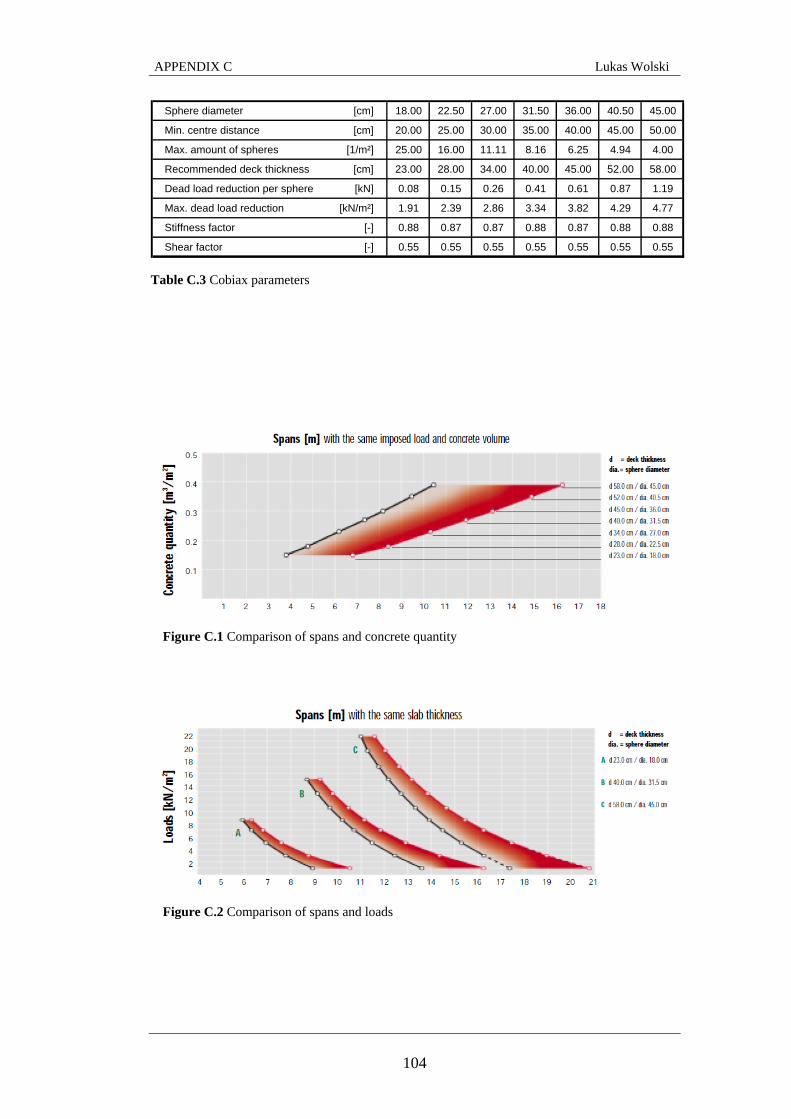
APPENDIX C Lukas Wolski
104
Sphere diameter [cm] 18.00 22.50 27.00 31.50 36.00 40.50 45.00
Min. centre distance [cm] 20.00 25.00 30.00 35.00 40.00 45.00 50.00
Max. amount of spheres [1/m²] 25.00 16.00 11.11 8.16 6.25 4.94 4.00
Recommended deck thickness [cm] 23.00 28.00 34.00 40.00 45.00 52.00 58.00
Dead load reduction per sphere [kN] 0.08 0.15 0.26 0.41 0.61 0.87 1.19
Max. dead load reduction [kN/m²] 1.91 2.39 2.86 3.34 3.82 4.29 4.77
Stiffness factor [-] 0.88 0.87 0.87 0.88 0.87 0.88 0.88
Shear factor [-] 0.55 0.55 0.55 0.55 0.55 0.55 0.55
Table C.3 Cobiax parameters
Figure C.1 Comparison of spans and concrete quantity
Figure C.2 Comparison of spans and loads