Native Parallel Graphs - Home - TigerGraph...Native Parallel Graphs handle both read and write in...
89
1 Native Parallel Graphs The Next Generation of Graph Database for Real-Time Deep Link Analytics
Transcript of Native Parallel Graphs - Home - TigerGraph...Native Parallel Graphs handle both read and write in...

1
Native Parallel GraphsThe Next Generation of Graph Database
for Real-Time Deep Link Analytics

Native Parallel GraphsThe Next Generation of Graph Database
for Real-Time Deep Link Analytics
Yu Xu, PhD
Victor Lee, PhD
Mingxi Wu, PhD
Gaurav Deshpande
Alin Deutsch, PhD
Copyright 2018 TigerGraph, Inc. All rights reserved.

2
Chapter 1 Modern Graph Databases.............................................................................................................7
Key Benefits of a Graph Database..........................................................................................................................................8
Better, Faster Queries and Analytics...........................................................................................................................8
Simpler and More Natural Data Modeling..................................................................................................................8
Represent Knowledge and Learn More.....................................................................................................................8
Object-Oriented Thinking.............................................................................................................................................8
More Powerful Problem-Solving.................................................................................................................................9
Modern Graph Databases Offer Real-Time Speed at Scale...................................................................................................9
Concurrent Querying and Data Updates in Real-Time..............................................................................................9
Deep Link Analytics......................................................................................................................................................9
Dynamic Schema Change...........................................................................................................................................9
Effortless Multidimensional Representation......................................................................................................10
Advanced Aggregation and Analytics......................................................................................................................10
Enhanced Machine Learning and AI........................................................................................................................10
Comparing Graphs and Relational Databases.....................................................................................................................11
Storage Model............................................................................................................................................................11
Query Model................................................................................................................................................................11
Types of Analytics......................................................................................................................................................11
Real-Time Query Performance..................................................................................................................................11
Transitioning to a Graph Database.......................................................................................................................................12
Chapter 2 The Graph Database Landscape.................................................................................................13
The Graph Database Landscape...........................................................................................................................................13
Operational Graph Databases...............................................................................................................................................13
Knowledge Graph / RDF.........................................................................................................................................................14
Multi-Modal Graphs................................................................................................................................................................14
Analytic Graphs......................................................................................................................................................................15
Real-time Big Graphs.............................................................................................................................................................15
Making Sense of the Offerings..............................................................................................................................................15
Chapter 3 Real-time Deep Link Analytics....................................................................................................17
Introducing Real-time Deep Link Analytics..........................................................................................................................18
Examples of Real-time Deep Link Analytics.........................................................................................................................18

3
Risk & Fraud Control..................................................................................................................................................18
Multi-Dimensional Personalized Recommendations..............................................................................................19
Power Flow Optimization, Supply-Chain Logistics, Road Traffic Optimization................................................19
A Transformational Technology for Real-time Insights and Enterprise AI........................................................................20
Chapter 4 Differentiating Between Graph Databases..................................................................................21
Chapter 5 Native Parallel Graphs................................................................................................................24
Different Architectures Support Different Use Cases.........................................................................................................24
Graph Traversal: More Hops, More Insight...........................................................................................................................25
TigerGraph’s Native Parallel Graph Design..........................................................................................................................25
A Native Distributed Graph........................................................................................................................................25
Compact Storage with Fast Access.........................................................................................................................26
Parallelism and Shared Values.................................................................................................................................26
Storage and Processing Engines Written in C++...................................................................................................27
GSQL Graph Query Language...................................................................................................................................27
MPP Computational Model.......................................................................................................................................28
Automatic Partitioning..............................................................................................................................................28
Distributed Computation Mode................................................................................................................................28
High Performance Graph Analytics with a Native Parallel Graph.......................................................................................28
Chapter 6: Building a Graph Database on a Key-Value Store?....................................................................30
The Lure of Key-Value Stores................................................................................................................................................30
The Real Cost of Building Your Own Graph Database.........................................................................................................30
1. Data Inconsistency and Wrong Query Results....................................................................................................31
2. Architectural Mismatch with Slow Performance...............................................................................................32
3. Expensive and Rigid Implementation..................................................................................................................32
4. Lack of Enterprise Support...................................................................................................................................32
Summary.....................................................................................................................................................................33
Example: Updating a Graph...................................................................................................................................................33
What are Some Possible Graph Over Key-value Workarounds?........................................................................36
Chapter 7 Querying Big Graphs...................................................................................................................37
Eight Prerequisites for a Graph Query Language.................................................................................................................38
1 Schema-Based with Dynamic Schema Change...................................................................................................38

4
2 High-Level (Declarative) Graph Traversal.............................................................................................................39
3 Algorithmic Control of Graph Traversal................................................................................................................39
4 Built-in High-Performance Parallel Semantics....................................................................................................39
5 Transactional Graph Updates................................................................................................................................39
6 Procedural Queries Calling Queries.......................................................................................................................40
7 SQL User-Friendly....................................................................................................................................................40
8 Graph-Aware Access Control.................................................................................................................................40
How Does TigerGraph GSQL Address These Eight Prerequisites?.....................................................................................40
Schema-Based with Dynamic Schema Change.....................................................................................................40
High-Level (Declarative) Graph Traversal................................................................................................................41
Fine Control of Graph Traversal................................................................................................................................41
Built-in High-Performance Parallel Semantics........................................................................................................41
Transactional Graph Updates...................................................................................................................................41
Procedural Queries Calling Queries..........................................................................................................................41
SQL User-Friendly.......................................................................................................................................................41
Graph-Aware Access Control....................................................................................................................................42
Chapter 8 GSQL — The Modern Graph Query Language.............................................................................43
It’s Time for a Modern Graph Query Language....................................................................................................................43
What Should a Modern Graph Query Language Look Like?...............................................................................................44
Introducing GSQL...................................................................................................................................................................44
The Conceptual Descendent of MapReduce, Gremlin, Cypher, SPARQL and SQL............................................................45
SQL Inheritance..........................................................................................................................................................45
Map-Reduce Inheritance...........................................................................................................................................46
Gremlin Runtime Variable.........................................................................................................................................46
SPARQL Triple Pattern Match...................................................................................................................................46
Putting It All Together................................................................................................................................................46
GSQL 101 - A Tutorial.............................................................................................................................................................47
Data Set.......................................................................................................................................................................47
Prepare Your TigerGraph Environment....................................................................................................................48
Define a Schema........................................................................................................................................................49
Create a Vertex Type..................................................................................................................................................49
Create an Edge Type..................................................................................................................................................50

5
Create a Graph............................................................................................................................................................50
Load Data....................................................................................................................................................................51
Define a Loading Job.................................................................................................................................................52
Run a Loading Job.....................................................................................................................................................53
Query Using Built-In SELECT Queries......................................................................................................................54
Select Vertices............................................................................................................................................................54
Select Edges...............................................................................................................................................................57
Chapter 9 GSQL’s Capabilities Analyzed.....................................................................................................59
Example 1: Business Analytics - Basic.................................................................................................................................59
Example 2: Graph Algorithms................................................................................................................................................60
Advanced Accumulation and Data Structures.....................................................................................................................61
Example 3...............................................................................................................................................................................61
Multi-hop Traversals with Intermediate Result Flow...........................................................................................................62
Example 4...............................................................................................................................................................................62
Control Flow............................................................................................................................................................................63
Turing Completeness.............................................................................................................................................................64
GSQL Compared to Other Graph Languages........................................................................................................................64
Gremlin....................................................................................................................................................................................64
Cypher......................................................................................................................................................................................67
SPARQL...................................................................................................................................................................................69
Final Remarks.........................................................................................................................................................................71
Chapter 10 Real-Time Deep Link Analytics in the Real World.....................................................................72
Combating Fraud and Money Laundering with Graph Analytics.......................................................................................72
Graph Analytics for AML...........................................................................................................................................73
Example: E-payment Company.................................................................................................................................74
Example: Credit Card Company................................................................................................................................74
How Graph Analytics Is Powering E-commerce..................................................................................................................75
Delivering a Better Online Shopping Experience...And Driving Revenue...........................................................................76
Empowering E-Commerce with Real-Time Deep Link Analytics.........................................................................................77
Deep Link Analytics for Product Recommendations............................................................................................................77
Example: Mobile E-Commerce Company.................................................................................................................77

6
The Customer Connection.....................................................................................................................................................78
Electric Power System Modernization..................................................................................................................................78
Example: National Utility Company .........................................................................................................................79
Chapter 11 Graphs and Machine Learning .................................................................................................81
A Machine Learning Algorithm Is Only as Good as Its Training Data................................................................................81
More Data Beats Better Algorithms......................................................................................................................................82
Building a Better Magnet for Phone-Based Fraud................................................................................................................82
Building a Better Magnet for Anti-Money Laundering..........................................................................................................85
Example: E-payment Company..............................................................................................................................................86
Example: Credit Card Company.............................................................................................................................................86
Conclusion.....................................................................................................................................88

7
Chapter 1
Modern Graph DatabasesGraph databases are the fastest growing category in all of data management. Since seeing early adoption by companies including Twitter, Facebook and Google, graphs have evolved into a mainstream technology used today by enterprises in every industry and sector. By organizing data in a graph format, graph databases overcome the big and complex data challenges that other databases cannot. Graphs offer clear advantages over both traditional RDBMSs and newer NoSQL big data products.
A graph database is a data management software application. The building blocks are nodes (also known as
vertexes or vertices) and edges (connections between nodes). A social graph is a simple example of a graph. To
put this in context, a relational database is also a data management software application in which the building
blocks are tables. Both require loading data into the software and using a query language or APIs to access the
data.
Relational databases boomed in the 1980s. Many commercial companies (e.g., Oracle, Ingres, IBM) backed the
relational model (tabular organization) of data management. In that era, the main data management need was to
generate reports.
But the requirements for data management have changed. The explosive volume and velocity of data, more
complex data analytics, frequent schema changes, real-time query response time, and more intelligent data

8
activation requirements have made people realize the advantages of the graph model.
Commercial software companies have been backing this model for many years, including TigerGraph, Neo4j, and
DataStax’s DSE Graph. The technology is disrupting many areas, such as supply chain management, e-commerce
recommendations, cybersecurity, fraud detection, and many other areas in advanced data analytics.
Key Benefits of a Graph Database
Any well-defined graph database has advantages over relational and NoSQL databases. In the following chapters,
we’ll examine the differences between different graph databases.
Better, Faster Queries and Analytics
Graph databases offer superior performance for querying related data, big or small. The graph model offers
an inherently indexed data structure, so it never needs to load or touch unrelated data for a given query.
This efficiency makes it an excellent solution for better and faster real-time big data analytical queries. This
is in contrast to NoSQL databases such as MongoDB, HBase/HDFS (Hadoop), and Cassandra, which have
architectures built for data lakes, sequential scans, and the appending of new data (no random seek). The
assumption in such systems is that every query touches the majority of a file. The situation is even worse in
relational databases, which are slow at processing full tables and yet need to join tables together in order see
connections.
Simpler and More Natural Data Modeling
Anyone who has studied relational database modeling understands the strict rules for satisfying database
normalization and referential integrity. Some NoSQL architectures go to the other extreme, pulling all types of data
in one massive table. In a graph database, on the other hand, you are free to define whatever node types you want,
and free to define edge types to represent relationships between vertices. A graph model has exactly as much
semantic meaning as you want, with no normalization and no waste.
Represent Knowledge and Learn More
Knowledge graphs are, of course, graphs. A knowledge graph is an assemblage of individual facts represented in
the form <subject><predicate><object>, such as <Pat><owns><boat>. With <subject> and <object> as nodes and
<predicate> as the edge between them, you have a graph. The real power of a knowledge graph is to see the big
picture: follow a chain of edges, analyze a neighborhood, or analyze the entire graph. From that, you can deduce or
infer new relationships.
Object-Oriented Thinking
In a graph, each node and edge is a self-contained object instance. In a schema-based graph database, the user
defines node types and edge types, just like object classes. Moreover, the edges which connect a node to others

9
are somewhat like object methods, because they describe what the node can “do.” To process data in a graph, you
“traverse” the edges, conceptually traveling from node to adjacent node, maintaining the integrity of the data. In a
relational database, in contrast, to connect two records, you must join them and create a new type of data record.
More Powerful Problem-Solving
Graph databases solve problems that are both impractical and practical for relational queries. Examples include
iterative algorithms such as PageRank, gradient descent, and other data mining and machine learning algorithms.
Some graph query languages are Turing complete, meaning that you can write any algorithm on them. There are
many query languages in the market that have limited expressive power, though.
Modern Graph Databases Offer Real-Time Speed at Scale
As stated above, graph databases offer better modeling which in turn leads to better problem-solving for
interconnected data. But a historical weakness of graph databases has been poor scalability: they cannot load
or store very large datasets, cannot process queries in real time, and/or they cannot traverse more than two
connections in series (two hops) in a query.
However, a new generation of graph database is now available. Based on Native Parallel Graph architecture, this
3rd generation graph has the speed and scalability to provide the following benefits:
Concurrent Querying and Data Updates in Real-Time
Many past graph systems could not ingest new data in real-time, because they were built on NoSQL data stores
designed for good read performance at the cost of write performance. But many applications, such as fraud
detection and personalized real-time recommendation, and any transactional or streaming data application,
demand real-time updates. Native Parallel Graphs handle both read and write in real-time. Typically the parallelism
is coupled with concurrency control to provide high queries-per-second for both read queries and graph updates.
Deep Link Analytics
One of the most important gains achieved by Native Parallel Graph design is the ability to handle queries that
traverse many, many hops, 10 or more, on very large graphs and in real time. The combination of the native graph
storage (which makes each data access faster) and parallel processing (which handles multiple operations at the
same time) transforms many use cases from impossible to possible.
Dynamic Schema Change
In principle, a graph model lets you describe new types of data and new types of relationships by simply defining
new node types and edge types. Or you may want to add or subtract attributes. You can connect multiple datasets
by simply loading them together any adding some new edges to connect them. The ease with which this can be
done varies in practice. Native Parallel Graphs, because they are graphs from the ground up and are designed with

10
graph schema evolution in mind, can handle such schema changes dynamically — that is, while the graph remains
in use.
Effortless Multidimensional Representation
Suppose you want to add geolocation attributes to entities. Or you want to record time series data. Of course you
can do this with a relational database. But with a graph database, you can choose to treat Location and Time as
node types as well as attributes. Or you can use weighted edges to explicitly link entities that are close together,
in space or time. You can create a chain of edges to represent a causal change. Unlike the relational model, you
do not need to create a cube to represent multiple dimensions. Every new node type and edge type represents a
potential new dimension; actual edges represent actual relationships. The possibilities are endless.
Advanced Aggregation and Analytics
Native Parallel Graph databases, in addition to traditional group-by aggregation, can do more complex
aggregations that are unimaginable or impractical in relational databases. Due to the tabular model, aggregate
queries on a relational database are greatly constrained by how data are grouped together. In contrast, the multi-
dimensional nature of graphs and the parallel processing of modern graph databases let the user efficiently slice,
dice, rollup, transform, and even update the data — without the need to preprocess the data or force it into a rigid
schema.
Enhanced Machine Learning and AI
We have already mentioned that graphs can be used as knowledge graphs, which allow one to further infer
indirect facts and knowledge. Moreover, any graph is a powerful asset for better machine learning. First, for
unsupervised learning, the graph model provides an excellent way to detect clusters and anomalies, because you
just need to pay attention to the connections. For supervised learning, which is always hungry for more and better
training data, graphs provide an excellent source of previously overlooked features. For example, simple features
such as the outdegree of an entity or the shortest path between two entities could provide the missing piece to
boost predictive accuracy. Then if the machine-learning/AI application requires real-time decision-making, we need
a fast graph database. The keys to a successful graph database to serve as a real-time AI data infrastructure are:
y Support for real-time updates as fresh data streams in
y A highly expressive and user-friendly declarative query language to give full control to data scientists
y Support for deep-link traversal (>3 hops) in real-time (sub-second), just like human neurons sending
information over a neural network
y Scale out and scale up to manage big graphs
There are many advantages of native graph databases managing big data that cannot be worked around by
traditional relational databases. However, as any new technology replacing old technology, there are still obstacles
in adopting graph databases. This includes the non-standardization of the graph database query language. There
have been incomplete offerings that have led to subpar performance and subpar usability, which has slowed down

11
graph model adoption.
Comparing Graphs and Relational Databases
Storage Model
An RDBMS stores information in tables (rows/columns). Typically, there is a table for each type of entity (e.g.,
Student, Instructor, Course, Semester, Registration). In the real world, there could be dozens or even hundreds of
tables in an RDBMS.
In a graph database, all information is stored as a collection of nodes and edges (connections between nodes),
not in physically separated tables. For example, a user can be represented as a node which is directly connected
to several other nodes: the user’s phone number, home address, purchased products, friends, etc. Each node and
each edge can store a set of attributes.
Query Model
The RDBMS fundamental computational model is based on scanning rows, joining rows, filtering rows, and
aggregation.
A graph database’s computational model is based on starting from an initial set of nodes and traversing the graph
in a series of hops. Each hop moves from the current set of nodes and follows a selected subset of connections
(edges) to their neighboring nodes. The query’s details specify where to start, which edges and destination nodes
to select, how many hops to take, and what to do with the data observed during the traversal.
Types of Analytics
Relational databases are good at accounting, simple data lookup that involves one, two, or at most three
tables, and descriptive statistics. However, they are not well-suited for more discovery- or prediction- oriented
analytics. For example, it’s hard or impossible to write a SQL query to answer questions like “How are these three
users connected?”, “How much money eventually flows from an account A to another 3 accounts?”, “What
is the shortest/cheapest route between Point A and Point B?”, or “What is the downstream consequences if a
component C in a network is out of service?” In a graph database system, all the above types of analytics can be
naturally and efficient expressed and solved.
Real-Time Query Performance
In a relational database, each table is stored physically separately, so following a connection from one table
to table is relatively slow. Moreover, if the database designer did not index their foreign keys, following the
connections will be VERY slow. In a graph database, everything about a node is connected to the node already,
thus the query performance can be significantly faster.

12
Transitioning to a Graph Database
With the Tigergraph native parallel graph database, setting up a basic graph schema and loading data into it are
very simple. If you already have a well-normalized relational schema, it is trivial to convert it to a workable graph
schema. After all, your entity-relationship model is a graph, right? The most challenging step will be learning to
think about your problem solving (querying) from a graph perspective (based on traversing from node to node)
instead of from a relational perspective (based on joining tables, projecting, and grouping to provide an output
table). For many applications, it is actually more natural and intuitive to think in the graph world, especially when
all information are already connected together in a graph.
TigerGraph provides GraphStudio UI, a complete end-to-end SDK, as well as GSQL, a high level language to make
developing a solution on top of the TigerGraph platform as smooth as possible and to make the steps very
compatible with the SQL world. You can follow this three-step process:
1. Create a graph model (very similar to SQL “create table”)
2. Load initial data into graph (simple declarative statements if your data is tabular)
3. Write a graph solution using GSQL. The syntax is modeled after SQL, enhanced with concepts from high
level procedural languages and MapReduce.
The knowledge and skills from the RDBMS domain are transferable to the TigerGraph world, especially in the
first two steps. TigerGraph’s extensive documentation and training materials provides numerous examples from
various verticals and use cases to illustrate these three steps, applied to cases such as collaborative filtering
recommendation, content-based recommendation, graph algorithms like PageRank, and fraud investigation. You
will see that the direct translation of the relational schema to graph schema is not always the best choice.
Moreover, in the TigerGraph system, the graph is also a distributed computational model: you can associate a
compute function with nodes and edges. Logically, nodes and edges aren’t just pieces of static data anymore;
they become active computing elements, similar to neurons in our brains. Nodes can send messages to other
nodes via edges. Once you learn to “think like a graph”, a new world of possibilities will be open to you.

13
Chapter 2
The Graph Database LandscapeThe Graph Database Landscape
With the popularity of graph databases, many new players are emerging, creating a diverse landscape of tools and technologies. Let’s take a close look at the graph database landscape, defined by categories and leading solutions.
Graph databases are the fastest growing category in all of data management, according to consultancy DB-
Engines.com. A recent Forrester survey showed that 51 percent of global data and analytics technology decision-
makers are employing graph databases.
All other database types (RDBMS, data warehouse, document DB, and key-value DB) started primarily on-premises
and were welcomed before database-as-a-service was established. Now that the large cloud service providers are
going all in on graph technology, graph database adoption is likely to keep accelerating.
Many different kinds of graph database offerings are available today and each offers unique features and
capabilities, so it’s important to understand the differences.
Operational Graph Databases
According to Gartner, Operational Databases (not limited to graph databases) are “DBMS products suitable
for a broad range of enterprise-level transactional applications, and DBMS products supporting interactions
and observations as alternative types of transactions.” (Gartner Inc., Magic Quadrant for Operational Database
Management Systems, published: October 2016, ID: G00293203). Bloor Research states these solutions may
be either native graph stores or built on top of a NoSQL platform. They are focused at transactions (ACID) and
operational analytics, with no absolute requirement for indexes. (Bloor Research: Graph and RDF databases 2015
#2, published Sept. 2015)
Operational Graph Databases include Titan, JanusGraph, OrientDB, and Neo4j.

14
Knowledge Graph / RDF
The Resource Description Framework (RDF) is a family of World Wide Web Consortium specifications originally
designed as a metadata model. It has come to be used as a general method for conceptual description or
modeling of information that is implemented in web resources, using a variety of syntax notations and data
serialization formats. Each individual fact is a triple (subject, predicate, object), so RDF databases are sometimes
called triplestores.
According to Bloor Research, these graphs are often semantically focused and based on underpinnings (including
relational databases). They are ideal for use in operational environments, but have inferencing capabilities
and require indexes even in transactional environments. (Bloor Research: Graph and RDF databases 2015 #2,
published Sept. 2015)
A number of graph database vendors have based their knowledge graph technology on RDF, including
AllegroGraph, Virtuoso, Blazegraph, Stardog, and GraphDB.
Multi-Modal Graphs
This category encompasses databases designed to support more than one model types. For example, a common
possibility is a three-way option of document store, key value store or RDF/graph store. (Bloor Research: Graph
and RDF databases 2016, published Jan. 2017) The advantages of a multi-modal approach are that different types
of queries, such as graph queries and key-value queries can be run against the same data. The main disadvantage
is that the performance cannot match a dedicated and optimized database management system.

15
Examples of multi-modal graphs include Microsoft Azure Cosmos DB, ArangoDB and DataStax.
Analytic Graphs
Bloor Research states that analytic graphs focus on solving ‘known knowns’ problems (the majority) – where both
entities and relationships are known, or on ‘known unknowns’ and even ‘unknown unknowns.’ The research firm
says, “Multiple approaches characterize this area with different architectures including both native and non-native
stores, different approaches to parallelisation, and the use of advanced algebra.” (Bloor Research: Graph and RDF
databases 2015 #2, published Sept. 2015)
Examples of Analytic Graphs include Apache Giraph, Spark GraphX, and Turi (formerly GraphLab, now owned by
Apple).
Real-time Big Graphs
A new category of graph databases, called the real-time big graph, is designed to deal with massive data volumes
and data ingestion rates and to provide real-time analytics. To handle big and growing datasets, real-time big
graph databases are designed to scale up and scale out well.
Real-time big graphs enable real-time large graph analysis with both 100M+ node or edge traversals/sec/server
and 100K+ updates/sec/server, regardless of the number of hops traversed in the graph. They also provide real-
time graph analytic capabilities to explore, discover, and predict very complex relationships. This represents
Real-Time Deep Link Analytics - achieving 10+ hops of traversal across a big graph, along with fast graph traversal
speed and data updates.
Examples of Real-Time Big Graphs include TigerGraph.
Making Sense of the Offerings
In summary, there are many different kinds of graph database offerings available today and unique advantages
to each, which is why it’s important to understand the differences as graph databases continue to see adoption
by enterprises across every vertical and also use case. Per a recent Forrester Research survey, “51 percent of

16
global data and analytics technology decision makers either are implementing, have already implemented, or are
upgrading their graph databases.” (Forrester Research, Forrester Vendor Landscape: Graph Databases, Yuhanna, 6
Oct. 2017)
As organizations embrace the power of the graph, knowing offerings available and their advantages is important
to determine the best option for a particular use case. Demonstrated by the Real-Time Big Graphs category, graph
technology is evolving into the next-generation. These solutions are specifically designed to support real-time
analytics for organizations with massive amounts of data.
17
Chapter 3
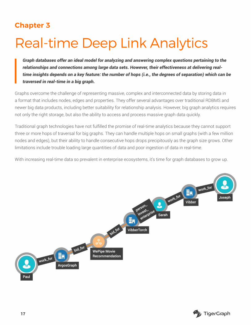
Real-time Deep Link AnalyticsGraph databases offer an ideal model for analyzing and answering complex questions pertaining to the relationships and connections among large data sets. However, their effectiveness at delivering real-time insights depends on a key feature: the number of hops (i.e., the degrees of separation) which can be traversed in real-time in a big graph.
Graphs overcome the challenge of representing massive, complex and interconnected data by storing data in
a format that includes nodes, edges and properties. They offer several advantages over traditional RDBMS and
newer big data products, including better suitability for relationship analysis. However, big graph analytics requires
not only the right storage, but also the ability to access and process massive graph data quickly.
Traditional graph technologies have not fulfilled the promise of real-time analytics because they cannot support
three or more hops of traversal for big graphs. They can handle multiple hops on small graphs (with a few million
nodes and edges), but their ability to handle consecutive hops drops precipitously as the graph size grows. Other
limitations include trouble loading large quantities of data and poor ingestion of data in real-time.
With increasing real-time data so prevalent in enterprise ecosystems, it’s time for graph databases to grow up.

18
Introducing Real-time Deep Link Analytics
Today’s enterprises demand real-time graph analytic capabilities that can explore, discover, and predict complex
relationships. This represents Real-Time Deep Link Analytics which is achieved utilizing three to 10+ hops of
traversal across a big graph, along with fast graph traversal speed and fast data updates.
Consider a simple personalized recommendation such as “customers who liked what you liked also bought these
items.” Starting from a person, the query first identifies items you’ve viewed / liked / bought.
Second, it finds other people who have viewed / liked / bought those items.
Third, it identifies additional items bought by those people.
Person → Product → (other)Persons → (other) Products
This query requires three hops in real time, so it is beyond the two-hop limitation of previous generations of graph
technology on larger data sets. Adding in another relationship (e.g, features of products, availability of products)
easily extends the query to four or more hops.
Examples of Real-time Deep Link Analytics
As each additional hop reveals new connections and hidden insight from within colossal amounts of data, Real-
Time Deep Link Analytics represents the next stage and evolution of graph analytics. In particular, Real-Time Deep
Link Analytics offers huge advantages for use cases including fraud prevention, personalized recommendation,
supply chain optimization, and other analysis capabilities needed for today’s most critical enterprise applications.
Here’s a look at how:
Risk & Fraud Control
Real-Time Deep Link Analytics combats financial crime by identifying high-risk transactions. For example, starting
from an incoming credit card transaction, how this transaction is related to other entities can be identified as
follows:
New Transaction → Credit Card → Cardholder → (other)Credit Cards → (other)Bad
Transactions
This query uses four hops to find connections only one card away from the incoming transaction. Today’s
fraudsters try to disguise their activity by having circuitous connections between themselves and known bad
activity or bad actors. Any individual connecting the path can appear innocent, but if multiple paths from A to
B can be found, the likelihood of fraud increases. Thus not only depth of traversal (4 hops) is needed, but also
breadth of traversal (finding multiple paths).

19
Given this, successful risk and fraud control requires the ability to traverse several hops.. This traversal pattern
applies to many other use cases — where you can simply replace the transaction with a web click event, a phone
call record or a money transfer. With Real-Time Deep Link Analytics, multiple, hidden connections are uncovered
and fraud is minimized.
Multi-Dimensional Personalized Recommendations
Real-Time Deep Link Analytics enables queries to find similar customers or to provide personalized
recommendations for products. Consider the following examples of recommendation paths, all of which are
longer than three hops:
i
Person→ Purchases→ Products→ (other)Purchases→ (other)Persons→ (other)Products
Person → Purchases→ Products→ Categories→ (other)Products
Person→ Clicks→ Products→ Categories→ (other)Products
Any of the above paths can be used for personalized recommendations on a retail website, for example, either
individually or in combination with each other. The first path selects products bought by other users who bought
the same products you bought. The second determines products similar to the products you bought, and the
third determines products similar to the products you viewed/are interested in. A recommendation algorithm can
assign different weights at run time to products found in each type of path to give a user a mixed ensemble of
products for recommendation.
However, due to limitations in current systems, the vast majority of current recommendation functions use offline
computation. As recommendations are computed in the background they are unable to perform real-time, on-
demand analytics using the latest data. This has been a setback that new graph database technology is now able
to address.
Power Flow Optimization, Supply-Chain Logistics, Road Traffic Optimization
These applications adjust each entity and/or each connection, until a dynamic equilibrium or optimization is
established. For example, in a national or regional power grid, the power output of each generator is adjusted as
follows:
All Entities:
→ relationship to and effect on neighbors
→ Update All Entities
<repeat until a stable state is achieved>.

20
Finding the right values inherently requires iterative computation in a graph (similar to PageRank) until some
metric values converge. Moreover, each top-level component (e.g., a power generator), is the hub for a network of
supporting elements, resulting in a multi-tier mesh. A power distribution network could easily have a six-hop path.
Power generator→ Transformers→ Control units→ Lower-level transformers→ Lower-
level control units→ Meters→ Power-consuming devices
Real-Time Deep Link Analytics is needed for a graph database system to handle this level of computation.
A Transformational Technology for Real-time Insights and Enterprise AI
What enterprises currently get from limited graph analytics is only the tip of iceberg compared to what Real-
Time Deep link Analytics can provide. By supporting all connections between data entities, Real-Time Deep Link
Analytics offers a truly transformative technology, particularly for organizations with colossal amounts of data.
The entry of Real-Time Deep Analytics represents a new era of graph analytic technology. As the next stage in the
graph database revolution, it is empowering users to explore, discover and predict relationships more accurately,
more quickly and with more insight than ever before. The result is real-time support for enterprise AI applications
– a true game changer in today’s competitive market moving at the pace of now.

21
Chapter 4
Differentiating Between Graph Databases
Graph databases have gotten much attention due to their advantages over relational models . With many vendors rushing into this area, it is becoming challenging to evaluate all the product offerings. Here is a list of what to consider when evaluating graph databases.
y Property graph or RDF store. RDF stores are specialty graph databases; property graphs are general
purpose. If your data are purely RDF and if your queries are limited to pattern matching or logical
inference, then you may be satisfied with an RDF database. Other users should focus on property graphs.
Even so, some enterprises with RDF knowledge graph applications have still turned to property graph
databases, because the performance of the available RDF databases was not strong enough.
y Loading capability. If you measure data in gigabits or larger, this is a critical differentiator. It is especially
important if you plan to routinely import different data from your data lake into your graph DB. Both
loading speed and usability are important. If you do not already have test data, consider a public data
set such as the 1.5B edge Twitter follower network (http://an.kaist.ac.kr/traces/WWW2010.html) or the
1.8B edge Friendster network (http://snap.stanford.edu/data/com-Friendster.html). First, does the graph
database require that you define a schema beforehand and if so, it is straightforward? Does it support the
data types, including composite types, that you need? Can the DB directly extract, transform, and load
(ETL) data from your data files, or do you need to preprocess your data? Can it handle multiple common
input file formats? How long does it take to load 10M edges? 20M edges? Does the database maintain
good loading speed as the graph grows? Does it support parallel loading, for better throughput? Does it
support scheduling and restart, which may be necessary for very large loading jobs? These questions will
jump-start your evaluation.
y Native graph storage. Many graph databases are non-native, meaning they store graph data in relational
tables, RDF triples, or key-value pairs on disk. When data are fetched to memory, they provide middle
layer APIs to simulate a graph view and graph traversal. In contrast, native graph databases store data
directly in a graph model format—nodes and edges. The most well-known examples of native graphs
are TigerGraph and Neo4j. Non-native graphs are a compromise solution. They can more easily support
a multi-modal database (presenting more than data model from one data store), by sacrificing graph
performance. On the other hand, the edge-and-node storage model of a native graph provides built-in
indexing, for quicker and more efficient graph traversal. When the dataset is large, non-native graphs
generally have difficulty handling queries with 3 or more hops.
y Schema or schema-less. Some graph databases claim they do not require a pre-defined schema. Other

22
graph databases require a predefined schema, following the model of traditional relational databases.
It may seem like schema-less is better (less work for the architect!) but there is a price in performance.
A predefined schema allows for more efficient storage, query processing, and graph traversal, so the
small initial effort to define a schema pays for itself many times over. However, if a predefined schema is
required, be sure that the database supports schema changes (preferably online, while the database is in
service). You can be sure that the initial schema you design will not be your final schema.
y OLTP, OLAP, or HTAP. What type of operations do you want your graph database to perform? Some graph
platforms are purely for large-scale processing (OLAP), such as PageRank or community detection. A
good OLAP graph database should have a highly parallel processing design and good scalability. Some
graph databases are designed for “point queries” - starting from one or a few nodes and traversing for a
few hops. To be a truly transactional database (for OLTP), however, it should support ACID transactions,
concurrency, and a high number of queries per second (QPS). If the transactions include database
updates, then real-time updates is a must (see below). A very few graph databases satisfy both of these
requires and so can be considered Hybrid Transactional/Analytical Processing (HTAP) databases.
y Real-time update. Real-time update means that a database update (add, delete, or modify) can happen
at the same time as other queries on the database, and also that the update can finish (commit) and
be available quickly. Common graph update operations include insertion/deletion of a new node/edge
and update of an attribute of an existing node/edge. Ideally, real-time update should be coupled with
concurrency control, such that multiple queries and updates (transactions) can run simultaneously, but
the end results are the same as if the transactions had run sequentially. Most non-native graph platforms
(e.g., GraphX, DataStax DSE Graph) do not support real-time update due to the immutability of their data
storage systems (HDFS, Cassandra).
y Real-time deep-link analytics. On most graph databases today, query response time degrades
significantly starting from three hops. Yet the real value of a graph database is to find those non-
superficial connections which are several hops deep. A simple way to check a graph database’s deep link
performance is to run a series of k-hop neighborhood size queries for increasing values of k, on a large
(~1B edge) graph. That is, find all the nodes which are one hop away from a starting node, then two hops,
three hops, and so on. To focus on graph traversal and not on IO time, return only the number of k-hop
neighbors.
y Scalability with performance. Scalability is an important feature in the Big Data era. There is always
more data out there, and the more/richer/fresher data you have, the better analytics and insights you will
be able to produce. Users need assurance that their database will be able to grow. Database scalability
can be broken down into three main concerns:
• Software support - Are there software limits to the number of entities or size of data that can be
managed?
• Hardware configuration - Can the database take advantage of increased hardware capacities on
a single machine (scale up)? Can the database be distributed across an ever-growing cluster of

23
machines (scale out)?
• Scale-up performance - In a perfect system, if the data, memory and disk space all increase by a
factor of S, then the full graph loading time should increase by a factor of S, point query QPS should
remain about the same, and analytic (full graph) query time should increase according to the
algorithm’s computational complexity. That is, we expect things to run slower, but only due to the
fact that there is more data to process.
• Scale-out performance - In a perfect system, if the data and number of machines both increase by
a factor of S, then full graph loading time should remain constant (more data and more machines
cancel each other out), the point query QPS should increase by up to S (an improvement), and
the analytic (full graph) query time should increase according to the algorithm’s computational
complexity, divided by S. For example, if a graph grows to have 2x edges on 2x machines,
PageRank ideally takes the same amount of time, because PageRank’s computational effort scales
with the number of edges. Because machine-machine data transfer is slower than intra-machine
transfer, no system achieves this perfect mark, but you can compare systems to see how close
they come to the ideal standard. Note: Some databases with good parallel design can scale with
the number of cores in a CPU. This is technically scale-up, but its behavior is more similar to that of
scale-out.
y Enterprise Requirements. Besides the basic features of the graph database itself, enterprises need
support for security, reliability, maintenance, and administration. Many of these requirements are
identical to the requirements for traditional databases: role-based access control, encryption, multiple
tenancy, high availability, backup and restore, etc. However, since the graph database market is less
mature, not all vendors have a comprehensive set of enterprise features. Customers may be willing to be
flexible for some of these requirements to obtain the unique advantages of graph databases.
y Graph Visualization. A final factor here is one that is unique to graph databases: the ability to display
a graph, either as an included capability or supported by a third party tool. A good visual display
greatly aids in the interpretation of the data. How large a graph can be displayed, and how is the layout
determined? Does the visualization system also support graph exploration or querying?
Graph databases are hot, so the market is offering consumers many choices. Regardless of your requirements,
considering each of the factors above will help you select the right graph database system.

24
Chapter 5
Native Parallel GraphsDifferent Architectures Support Different Use Cases
Whether for customer analytics, fraud detection, risk assessment, or another real-world challenge, the ability to quickly and efficiently explore, discover and predict complex relationships is a huge competitive differentiator for businesses today. Getting it done involves more than merely having connected data – it’s about real-time and up-to-date correlation, detection and discovery. Organizations need to be able to transform structured, semi-structured and unstructured data and massive enterprise data silos into an intelligent, interconnected, and operational data network that can reveal critical patterns and insights to support business goals.
This elemental pain point – the need for real-time analytics for enterprises with enormous volumes of data – is
fueling graph databases’ emergence as a mainstream technology being embraced by companies across a broad
range of industries and sectors.
Since seeing early adoption by companies including Twitter, Facebook and Google, graph databases are heating
up. Giant cloud service providers Amazon, IBM and Microsoft have added graph databases in the last two years,
validating the industry’s growing interest in graph technology for easy and natural data modeling, easy-to-write
queries to solve complex problems, and fast insights from interconnected data.
Graph databases excel at answering complex questions about relationships in large data sets. But most of them
hit a wall—in terms of both performance and analysis capabilities—when the volume of data grows very large, or
the problem needs deep link analytics, or when the answers must be provided in real time.
That’s because earlier generations of graph databases lack the technology and design for today’s speed and scale
requirements. First generation designs (such as Neo4j) were not built with parallelism or distributed database
concepts in mind. The second generation is characterized by creating a graph view on top of a NoSQL store.
These products can scale to large size, but the added layer robs them of much potential performance. It is costly
to perform multi-hop queries without a native graph design, and many NoSQL platforms are designed for read
performance only. They do not support real-time updates.
TigerGraph represents a new generation in graph database design - the native parallel graph, overcoming the
limitations of earlier generations. Native parallel graph enables deep link analytics, which offers the following
advantages:
y Faster data loading to build graphs quickly

25
y Faster execution of graph algorithms
y Real-time capability for streaming updates and insertions
y Ability to unify real-time analytics with large-scale offline data processing
y Ability to scale up and scale out for distributed applications
Graph Traversal: More Hops, More Insight
Why deep link analytics? Because the more links you can traverse (hop) in a graph, the greater the insight you
achieve. Consider a hybrid knowledge and social graph. Each node connects to what you know and who you know.
Direct links (one hop) reveal what you know. Two hops reveal everything that your friends and acquaintances
know. Three hops? You are on your way to revealing what everyone knows.
The graph advantage is knowing the relationships between the data entities in the data set, which is the heart
of knowledge discovery, modeling, and prediction. Each hop can lead to an exponential growth in the number of
connections and, accordingly, in the amount of knowledge. But therein lies the technological hurdle. Only a system
that performs hops efficiently and in parallel can deliver real-time deep link (multi-hop) analytics.
In Chapter 3, we took a detailed look at real-time deep link analytics and some of the use cases where it adds
unique value: risk and fraud control, personalized recommendations, supply chain optimization, power flow
optimization, and others.
Having seen the benefits of a native parallel graph, now we’ll take a look at how it actually works.
TigerGraph’s Native Parallel Graph Design
The ability to draw deep connections between data entities in real time requires new technology designed for
scale and performance. Not all graph databases claiming to be native or to be parallel are created the same. There
are many design decisions which work cooperatively to achieve TigerGraph’s breakthrough speed and scalability.
Below we will look at these design features and discuss how they work together.
A Native Distributed Graph
TigerGraph is a pure graph database, from the ground up. Its data store holds nodes, links, and their attributes,
period. Some graph database products on the market are really wrappers built on top of a more generic NoSQL
data store. This virtual graph strategy has a double penalty when it comes to performance. First, the translation
from virtual graph operation to physical storage operation introduces extra work. Second, the underlying structure
is not optimized for graph operations. Moreover, the database is designed from the beginning to support scale out.

26
Compact Storage with Fast Access
TigerGraph isn’t described as an in-memory database, because having data in memory is a preference but not a
requirement. Users can set parameters that specify how much of the available memory may be used for holding
the graph. If the full graph does not fit in memory, then the excess is stored on disk. Best performance is achieved
when the full graph fits in memory, of course.
Data values are stored in encoded formats that effectively compress the data. The compression factor varies with
the graph structure and data, but typical compression factors are between 2x and 10x. Compression has two
advantages: First, a larger amount of graph data can fit in memory and in CPU cache. Such compression reduces
not only the memory footprint, but also CPU cache misses, speeding up overall query performance. Second, for
users with very large graphs, hardware costs are reduced. For example, if the compression factor is 4x, then an
organization may be able to fit all its data in one machine instead of four.
Decompression/decoding is very fast and transparent to end users, so the benefits of compression outweigh the
small time delay for compression/decompression. In general, decompression is needed only for displaying the
data. When values are used internally, often they may remain encoded and compressed.
Internally hash indices are used to reference nodes and links. In Big-O terms, our average access time is O(1) and
our average index update time is also O(1). Translation: accessing a particular node or link in the graph is very fast,
and stays fast even as the graph grows in size. Moreover, maintaining the index as new nodes and links are added
to the graph is also very fast.
Parallelism and Shared Values
When speed is your goal, you have two basic routes: Do each task faster, or do multiple tasks at once. The latter
avenue is parallelism. While striving to do each task quickly, TigerGraph also excels at parallelism, employing an
MPP (massively parallel processing) design architecture throughout. For example, its graph engine uses multiple
workers and threads to traverse a graph, and it can employ each core in a multicore CPU.
The nature of graph queries is to “follow the links.” Start from one or more nodes. Look at the available
connections from those nodes and follow those connections to some or all of the neighboring nodes. We say you
have just “traversed” one “hop.” Repeat that process to go to the original node’s neighbors’ neighbors, and you have
traversed two hops. Since each node can have many connections, this two-hop traversal involves many paths to
get from the start nodes to the destination nodes. Graphs are a natural fit for parallel, multithreaded execution.
A query of course should do more than just visit a node. In a simple case, we can count the number of unique two-
hop neighbors or make a list of their IDs. How does one compute a total count, when you have multiple parallel
counters? The process is similar to what you would do in the real world: Ask each counter to do its share of the
world, and then combine their results in the end.
Recall that the query asked for the number of unique nodes. There is a possibility that the same node has been

27
counted by two different counters, because there is more than one path to reach that destination. This problem
can occur even with single-threaded design. The standard solution is to assign a temporary variable to each
node. The variables are initialized to False. When one counter visits a node, that node’s variable is set to True, so
that other counters know not to count it. The explanation here may sound complex, you can actually write these
type of graph traversal with counting and more complex computations in a few lines of code (shorter than this
paragraph) using TigerGraph’s high level query language.
Storage and Processing Engines Written in C++
Language choices also affect performance. TigerGraph’s graph storage engine and processing engine are
implemented in C++. Within the family of general purpose procedural languages, C and C++ are considered lower-
level compared to other languages like Java. What this means is that programmers who understand how the
computer hardware executes their software commands can make informed choices to optimize performance.
TigerGraph has been carefully designed to use memory efficiently and to release unused memory. Careful memory
management contributes to TigerGraph’s ability to traverse many links, both in terms of depth and breadth, in a
single query.
Many other graph database products are written in Java, which has pros and cons. Java programs run inside a
Java Virtual Machine (JVM). The JVM takes care of memory management and garbage collection (freeing up
memory that is no longer needed). While this is convenient, it is difficult for the programmer to optimize memory
usage or to control when unused memory becomes available.
GSQL Graph Query Language
TigerGraph also has its own graph querying and update language, GSQL. While there are many nice details about
GSQL, there are two aspects that are key to supporting efficient parallel computation: the ACCUM clause and
accumulator variables.
The core of most GSQL queries is the SELECT statement, modeled closely after the SELECT statement in SQL.
The SELECT, FROM, and WHERE clauses are used to select and filter a set of links or nodes. After this selection,
the optional ACCUM clause may be used to define a set of actions to be performed by each link or adjacent node. I
say “perform by” rather than “perform on” because conceptually, each graph object is an independent computation
unit. The graph structure is acting like a massively parallel computational mesh. The graph is not just your data
storage; it is your query or analytics engine as well.
An ACCUM clause may contain many different actions or statements. These statements can read values from
the graph objects, perform local computations, apply conditional statements, and schedule updates of the
graph.To support these distributed, in-query computations, the GSQL language provides accumulator variables.
Accumulators come in many flavors, but they are all temporary (existing only during query execution), shared
(available to any of the execution threads), and mutually exclusive (only one thread can update it at a time).
For example, a simple sum accumulator would be used to perform the count of all the neighbors’ neighbors
mentioned above. A set accumulator would be used to record the IDs of all those neighbors’ neighbors.

28
Accumulators are available in two scopes: global and per-node. In the earlier query example, we mentioned the
need to mark each node as visited or not. Here, per-node accumulators would be used.
MPP Computational Model
To reiterate what we have revealed above, the TigerGraph graph is both a storage model and a computational
model. Each node and link can be associated with a compute function. Therefore, each node or link acts as a
parallel unit of storage and computation simultaneously. This would be unachievable using a generic NoSQL data
store or without the use of accumulators.
Automatic Partitioning
In today’s big data world, enterprises need their database solutions to be able to scale out to multiple machines,
because their data may grow too large to be stored economically on a single server. TigerGraph is designed to
automatically partition the graph data across a cluster of servers, and still perform quickly. The hash index is used
to determine not only the within-server data location but also which-server. All the links that connect out from a
given node are stored on the same server.
Distributed Computation Mode
TigerGraph has a distributed computation mode that significantly improves performance for analytical queries
that traverse a large portion of the graph. In distributed query mode, all servers are asked to work on the query;
each server’s actual participation is on an as-needed basis. When a traversal path crosses from server A to server
B, the minimal amount of information that server B needs to know is passed to it. Since server B already knows
about the overall query request, it can easily fit in its contribution.
In a benchmark study, we tested the commonly used PageRank algorithm. This algorithm is a severe test of a
graph’s computational and communication speed because it traverses every link, computes a score for every
node, and repeats this traverse-and-compute for several iterations. When the graph was distributed across eight
servers compared to a single-server, the PageRank query completed nearly seven times faster.
High Performance Graph Analytics with a Native Parallel Graph
TigerGraph represents a new era of graph technology that empowers users with true real-time analytics. The
technical advantages support more sophisticated, personalized, and accurate analytics, as well as enable
organizations to keep up with rapidly changing and expanding data.
As the world’s first and only true native parallel graph (NPG) system, TigerGraph is a complete, distributed, graph
analytics platform supporting web-scale data analytics in real time. The TigerGraph NPG is built around both
local storage and computation, supports real-time graph updates, and serves as a parallel computation engine.
TigerGraph ACID transactions, guaranteeing data consistency and correct results. Its distributed, native parallel
graph architecture enables TigerGraph to achieve unequaled performance levels:

29
y Loading 100 to 200 GB of data per hour, per machine.
y Traversing hundreds of million of nodes/edges per second per machine.
y Performing queries with 10-plus hops in subsecond time.
y Updating 1000s of nodes and edges per second, hundreds of millions per day.
y Scaling out to handle unlimited data, while maintaining real-time speeds and improving loading and
querying throughput.
The introduction of native parallel graphs is a milestone in the history of graph databases. Though this technology,
the first real-time deep link analytics database has become a reality.
30
Chapter 6:
Building a Graph Database on a Key-Value Store?
Until recently, graph database designs fulfilled some but not all of the graph analytics needs of enterprises. The first generation of graph databases (e.g., Neo4j) was not designed for big data. They cannot scale out to a distributed database, are not designed for parallelism, and perform slowly at both data loading and querying for large datasets and/or multi-hop queries.
The second generation of graph databases (e.g., DataStax Enterprise Graph) was built on top of NoSQL storage
systems such as Apache Cassandra. This addressed the scale-out issue, but since they lack a native graph
storage design, they still have slow performance for graph updates or multi-hop queries on large datasets. Faced
with the apparent lack of a high-performance graph database solution, some organizations have considered
building their own in-house graph solution. Rather than starting from scratch, a modern fast key-value store
seems like a good base on which to build a custom graph solution.
The Lure of Key-Value Stores
The NoSQL revolution came about because relational databases were too slow and too inflexible. Big data users
needed to ingest a variety of differently structured data, with both high volume and high velocity, and to scale out
their physical infrastructure with minimal fuss. The key-value store arose as the simplest and therefore fastest
NoSQL architecture. A key-value database is basically a two-column hash table, where each row has a unique key
(ID) and a value associated with that key. Searching the key field can return single data values very quickly, much
faster than a relational database. Key-value stores also scale well to very large data sets. Key-value stores are well
understood, and many free open-source designs are available. It seems fairly straightforward to use a fast key-
value store to hold a graph’s node entities and edge entities, implement a little more logic, and call that a graph
database.
The Real Cost of Building Your Own Graph Database
Building your own graph database on top of a key-value store , let alone a high-performance one, is much harder
that it looks. Here are two obvious difficulties:
1. You are following the architectural principles of the 2nd generation graph databases, but you are trying to
improve upon those. Products such as DataStax Enterprise Graph have already optimized performance as
31
much as they can, given the inherent limitations of a non-native graph storage design.
2. What you really need is a complete database management system (DBMS), not just a graph database.
A database is just a collection of data organized in a specific way such that storing and retrieving data
are supported. A DBMS, on the other hand, is the complete application program for using and managing
data via a database. A DBMS typically includes support for defining a database model, inserting, reading,
updating, and deleting data, performing computational queries (not just reading the raw data), applying data
integrity checks, supporting transactional guarantees and concurrency, interacting with other applications,
and performing administrative functions, such as managing user privileges and security. A do-it-yourself
design will need to implement and verify all of these additional requirements.
Let’s examine some of the common problems in building a high performance graph on top of key-value storage.
1. Data inconsistency and wrong query results
2. Architectural mismatch with slow performance
3. Expensive and rigid implementation
4. Lack of enterprise support
1. Data Inconsistency and Wrong Query Results
Key value stores are typically highly optimized for high throughput and low latency of single-record reads/writes.
As a result, ACID (Atomicity, Consistency, Isolation, Durability) properties are guaranteed only at the single-record
level for most key value stores. This means that data consistency is at risk for any real-world transactional events
that involve the writing of multiple records (e.g., customer purchases, money transfers, a rideshare request).
Lack of data consistency means that queries that aggregate across two or more of these common multi-record
transactions can result in incorrect results.
Developers hoping to build a system that businesses can truly trust should realize that data consistency and
guaranteeing correct results is an all-or-nothing endeavour. There are no shortcuts for ACID properties. In a
graph system, one transaction will often need to create multiple nodes and add new connections/edges between
new or existing nodes, all within a single, all-or-nothing transaction. The easy way to guarantee ACID is to perform
only one operation at a time, locking out all other operations. But this results in very slow throughput.
In a high-performance design, a transaction must never interfere with, slow down, or block any other existing or
incoming read-only queries, even if they are traversing neighboring parts of the graph. If concurrent operations
are a business requirement, then developers need to design and engineer a non-blocking graph transactional
architecture where multiple key-value transaction support is added inside the distributed key-value system.
There are many stories of development teams trying to implement a shortcut workaround that inevitably led to
downstream data and query correctness issues.

32
2. Architectural Mismatch with Slow Performance
Queries involving single records are fast with a key-value store. But key-value store query speeds degrade
sharply as queries become more complex. With each hop in the graph traversal, the application has to send a key-
value retrieval command to the external key-value store. More hops generate more communication overhead and
result in slower query performance. And computation on the data, such as filtering, aggregation, and evidence-
gathering, cannot be completely pushed down to the key-value store. Instead, it must take place in the graph
application layer, which creates additional input and output transmission with the key-value store while bogging
down the query performance even more. Moreover, computing in the graph application layer instead of inside a
native parallel graph platform, is by default non-parallel. To match the parallelism in a Native Parallel Graph like
TigerGraph, developers would need to take on the extra burden of parallelizing the computation in a single
machine or take the even more extraordinary burden of scaling out the computation to multiple machines and
taking care of the scheduling, messaging, failover, and other requirements of a distributed system.
Enterprises that want a high-performance graph want a system that analyzes complex relationships and surfaces
hidden patterns, with fast query performance. To address these requirements, developers would need to do all of
the following: build a graph over key-value application that handles basic graph modeling (describing the structure
and behavior of a graph in general), implement basic graph data definition and data manipulation operations,
ensure transactional guarantees, and then develop application queries on top of that. That is, in-house developers
would need to implement an interpreter for a data definition language (DDL) and a graph query language.
Developers should consider the significant time and resources required to support such a challenging endeavor
and expect to deal with a lot of unforeseen downstream problem-solving.
3. Expensive and Rigid Implementation
Organizations thinking about creating their own graph database system on top of another database system
should consider the resources needed, reliability desired, and ideal adaptability of their application.
Building a graph on key-value system would take a great deal of time to complete. The upfront costs of building
custom software should not be underestimated. Furthermore, reliability is critical to application success. As
previously discussed, developers should put great thought into how they will design, test, deploy, and support a
graph ecosystem that includes full data consistency, correct results, and high performance of complex queries.
Finally, management and development teams should consider that a single application likely doesn’t have the
general purpose capabilities and flexibility of a high-performance distributed native graph database product.
Decision makers should consider the big picture and whether their custom design project can address unforeseen
future expansion. By choosing the right graph capabilities now, you can streamline tasks, reduce errors, and make
everyone’s life a lot easier for years to come.
4. Lack of Enterprise Support
Last but not least, a custom design will not include many of the features that are crucial for secure and reliable
enterprise deployment: user authorization and access control, logging, high availability, and integration with other
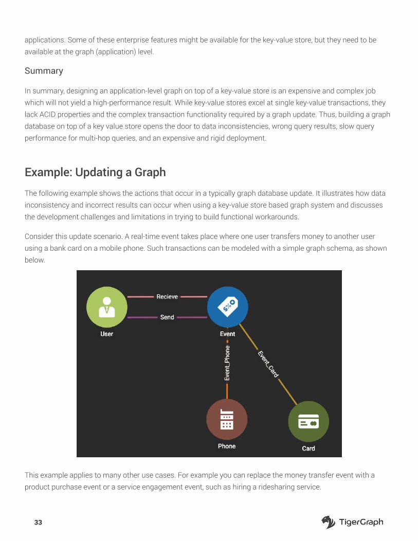
33
applications. Some of these enterprise features might be available for the key-value store, but they need to be
available at the graph (application) level.
Summary
In summary, designing an application-level graph on top of a key-value store is an expensive and complex job
which will not yield a high-performance result. While key-value stores excel at single key-value transactions, they
lack ACID properties and the complex transaction functionality required by a graph update. Thus, building a graph
database on top of a key value store opens the door to data inconsistencies, wrong query results, slow query
performance for multi-hop queries, and an expensive and rigid deployment.
Example: Updating a Graph
The following example shows the actions that occur in a typically graph database update. It illustrates how data
inconsistency and incorrect results can occur when using a key-value store based graph system and discusses
the development challenges and limitations in trying to build functional workarounds.
Consider this update scenario. A real-time event takes place where one user transfers money to another user
using a bank card on a mobile phone. Such transactions can be modeled with a simple graph schema, as shown
below.
This example applies to many other use cases. For example you can replace the money transfer event with a
product purchase event or a service engagement event, such as hiring a ridesharing service.

34
The money transfer event e1 can be described as the co-occurrence of four entities (u1, u2, c1, p1), where:
y u1 is the User sending money,
y u2 is the User receiving money,
y c1 is the payment Card used, and
y p1 is the Phone used.
For simplicity, we ignore all other attributes present in such event (like dollar amount, location, timestamp).
There are multiple ways to model a graph database with a graph over key-value system. One approach is to have
two tables in the graph over key-value system: a node table V and an edge table E. Another approach is to just
have a single node table (no edge table) which has a row for each node to store both node attributes and edge
information (edge attributes and connected nodes). The transaction challenges faced in either approach are
similar and are best illustrated using the two-table approach.
To update the graph by adding a new event e1, we perform the following actions:
1. For each entity u1, u2, c1, and p1, check if it already exists. Create a new node for each one that does not yet
exist ( named V_u1, V_u2, V_c1, V_p1). Equivalently in the graph over key-value system approach, we need to
insert from zero to four rows in the node table V.
2. Create a new node for event e1 (named V_e1 in the following discussion). Equivalently in the graph over key-
value system approach, we need to insert one row in the node table V.
3. Add four edges (from V_e1 to each of V_u1, V_u2, V_c1 and V_p1). To improve query performance, it may
be desirable to add an edge between V_u2 and V_c1 and another between V_u2 and V_p1. This will directly
connect all cards and phones used by a user but would make a graph over key-value system implementation
even more complex and error-prone.
Also we want to be able to find all events connected to a phone, a user, or a card. This requires adding four
additional edges in the other direction: from each of V_u1, V_u2, V_c1, and V_p1 to V_e1. Depending on the
implementation detail, this means either adding four rows, or updating the value of four existing rows. The
equivalent graph over key-value system approach would need to insert eight rows in the edge table E.

35
See the following example graph instance:
After the event e1 is processed and the graph is updated, the graph instance would look like the diagram above.
Since the event e1 is treated as a single transaction, the above three actions would happen to the graph
(equivalently to two tables) in an atomic way, which means that:
1. Either all three actions are guaranteed to be effective in the graph (or equivalently in two tables), or none
of them should be effective in the graph (or equivalently in two tables). A non-transactional system which
allows some but not all of the actions to take place (e.g., action 1 and 2 complete successfully but action
3 does not) leads to data inconsistency and wrong results. If any one or more actions do not complete, the
result will be missing edges with wrong query results.
2. During the time we apply actions 1, 2 and 3 and before they are completed, their effect should not be visible
to any other read or write operations. This means that if you have another query q1, which is still traversing
the edges/nodes in the graph before the event e1 comes into the system, q1 should not see any of the
actions of 1, 2 and 3 even if they complete successfully before e0 finishes.
3. This also means that if a read-only query q2 comes into the system later than e1 but before the three
actions of e1 are all completed, the effects of e1 should not be visible to q.

36
What are Some Possible Graph Over Key-value Workarounds?
A workaround is to simply ignore all data inconsistency and wrong query result issues and just insert key-value
rows to node table V and edge table E and hope for the best. Even if a company’s business requirements can be
relaxed to tolerate data inconsistency and wrong query results, this approach is going to face an implementation
nightmare. That is because the users don’t know whether or when they will miss a node or edge in the graph. To
address this, developers will need to tack on protection code to ensure the application will not hang or crash due
to traversing ghost/missing edges.
A better solution would be to add multiple key-value transaction support inside the distributed key-value system.
But this requires not only a huge amount of engineering effort but also significant slowdown of key-value
operations.
A third solution, a “placebo solution”, is to add some kind of locking mechanism inside the application level
without changing the kernel of the underlying key value store. Workarounds, like attempting to add a “commit”
flag to each row or maintaining a “dirty” list of rows in their applications, can reduce data inconsistencies and
incorrect results. However, such add-on features are not equivalent to an architecture designed for transactional
guarantees, so data inconsistencies and incorrect results may persist albeit hidden. Ensuring that these
workarounds consistently reconcile and address each transaction can be very difficult to guarantee.

37
Chapter 7
Querying Big Graphs
There are many property graph languages on the market, including Neo4j’s Cypher, Apache TinkerPop Gremlin, and TigerGraph’s GSQL, to name a few. Before discussing which graph language is the best, or how to fuse the best aspects of each graph language into a new, unified option, let’s take a step back to ask a more fundamental question: What are the prerequisites for a graph query language in the first place?
Our current era is witnessing a deluge of data — of interconnected data. The power of interconnected data to
provide transformative business value is proven by the emergence of giant internet companies, including Google
(knowledge graph), Facebook (social graph), LinkedIn (professional network), and Twitter (interest graph). Our
communication apps, electronic transactions, smart appliances, and monitoring devices generate enormous
volumes of connected data every second. A pressing demand for managing graph data has emerged.
For the first time in the history of databases, the relational model no longer works, because in relational databases

38
it is too slow to follow a chain of multiple connections. Each hop joins two tables, which is computationally
expensive. If you add indexes to the foreign keys, this will speed up the joins, but the general storage and
processing model for relational databases is still an impediment..
More importantly, SQL (the query language for relational databases) doesn’t even support a basic discovery
operation like “find all records linked by one connection,” because SQL requires that you know in advance what
type of entity is being targeted. Simply put, relational databases and the SQL language don’t work for discovery
and learning from connected data..
The graph model comes to the rescue by offering these beneficial features:
y Natural and efficient storage model for interconnected data.
y Natural model for managing evolving object types.
y Natural analytical and computational model for knowledge/inference/learning through chaining and
combining observations.
The graph database is the answer for managing and leveraging today’s vast and interconnected data. What is the
right query language for graphs?
Eight Prerequisites for a Graph Query Language
Just as SQL significantly lowered the barrier for managing relational data, a well-designed, user-friendly, and highly
expressive graph query language can significantly bridge the gap between asking high-level real world questions
and easily crafting a graph-based solution. To pick the right graph query language, let’s look at it from the point of
view of the users (developers) and the businesses they work for.
y Modeling: How do users want to model their graph data?
y Querying: What sort of results do organizations want to obtain from their graphs?
y Developing: How easy it is for developers to express their intent in the graph language?
These are all very high level questions, so to answer them we will break them down further. Below we present
eight prerequisites for a graph query language for today’s demanding needs.
1 Schema-Based with Dynamic Schema Change
A query language actual begins with the data structure it is querying. A strength of the graph model is the ease
with which it can reflect the natural organization of data objects. That data organization, or schema, is part of the
information. Accordingly, a good graph language should support well-defined schemas, containing user-defined
node types and edge types, each with its own set of characteristic properties or attributes. The language should
support a wide range of primitive and composite data types. Because data models change over time in the real
world, the language and system should also support easy and efficient schema changes, preferably while the

39
graph database remains online.
2 High-Level (Declarative) Graph Traversal
The SQL language is declarative, meaning users ask for data without worrying how the database software
executes the queries. This relieves the user from coding a step-by-step algorithm to perform their task. The same
paradigm can be applied to designing an elegant graph query language. For example, a simple query to “find this
pattern” should be expressed by defining the pattern and defining the search space. It should not have to explain
how to conduct the search.
3 Algorithmic Control of Graph Traversal
Graphs are capable of much more than simple search, so the query language must support this. Complex
analytics and data modifications, where at each hop, computations are performed, data may be updated, and
the next action depends on the current state, are possible. For example, consider classical graph algorithms
like PageRank, community detection, and centrality measurement, as well as applications like personalized
recommendation, fraud detection, supply chain optimization, and predictive analytics. Enterprises come to graph
management to design and execute complex algorithms that RDBMS and other NoSQL system cannot solve.
Therefore, in addition to declarative semantics, graph query languages also need to provide developers with
fine-grained algorithmic control of graph traverse-and-compute. In practice, if the language provides conditional
branching (“IF…THEN”), looping (“REPEAT”), and variables for temporary data storage, the language is Turing-
complete, capable of doing whatever a general purpose computer can do.
4 Built-in High-Performance Parallel Semantics
Graph algorithms are often expensive, as each hop could increase the data complexity exponentially. Let’s
consider how: starting from one node, the first hop can yield n neighbors, the next hop from the n immediate
neighbors can yield n² more neighbors, and so on. This exponential growth is why many graph databases can’t
handle more than two hops. To address this challenge, each traversal step in the graph should have built-in
parallel processing semantics to ensure high performance. To be sufficiently useful, parallel traversal needs to be
combined with a painless means of merging and aggregating.
5 Transactional Graph Updates
A full-featured graph query language needs to support more than just efficient graph reads, but also graph
writes (data insertions, updates, and deletions). That is, it should support more than just analytics (OLAP) but
also transactions (OLTP). A transactional database guarantees that if the user defines a block of operations to
be one transaction, then the transaction will complete in its entirety (or not all) and will not interact with any
other transactions which might be in process at the same time. The language must provide a way to define a
transaction, either implicitly or explicitly, as well as the insert, update, and delete operations.

40
6 Procedural Queries Calling Queries
As the tasks get more complex, good developers will want to apply one of the best ideas in programming to graph
queries: procedural programming. A procedure is a block of instructions that can be saved and “called” when
needed. Procedures provide modular design, hierarchical design, abstraction, code reuse, and better readability.
For example, consider a query that finds the most influential entity within a radius of K hops from the source node.
With procedural querying, this kHopInfluence procedure could be called and reused in multiple larger queries: for
recommendation, fraud investigation, optimization, etc. One of the cleverest ideas in algorithm design is recursion,
where a procedure calls itself. Depth-first search can be implemented nicely with recursion.
7 SQL User-Friendly
Most enterprises have developers who are familiar with SQL. The graph query language, therefore, should stay
close to SQL syntax and concepts as much as possible so that SQL developers can learn and implement graph
applications with minimal ramp-up time.
8 Graph-Aware Access Control
Enterprise customers are keen on facilitating collaboration with graph data. On one hand, they want a graph model
that can share selected parts of the data among multiple departments and even among partners. At the same
time, they also want to keep certain sensitive data private and accessible only by specific roles, departments
and partners, based on their business need. Graph schema-aware role-based access control is required for a
successful graph query language in the real world for large enterprises.
How Does TigerGraph GSQL Address These Eight Prerequisites?
Based on customer feedback over five years, TigerGraph has co-invented with our customers, over several
iterations, a Turing-complete graph query language called GSQL. It includes a DDL (Data Definition Language) for
defining a graph schema, a loading language for high-performance loading of structured and semi-structured data,
and a SQL-like graph traverse and compute language with inherent parallelism.
Schema-Based with Dynamic Schema Change
In GSQL, a Graph is defined as a collection of Vertex types and Edge types. One TigerGraph database may contain
multiple (possibly overlapping) graphs, each with its own set of user privileges and queries. E.g.,
CREATE VERTEX person (PRIMARY_ID ssn STRING, age INT, name STRING)
CREATE UNDIRECTED EDGE friendship (FROM person, TO person)
CREATE DIRECTED EDGE teacher_student (FROM person, TO person)
CREATE GRAPH School (person, friendship, teacher_student)
Also, GSQL’s DDL supports dynamic schema change with SQL-like syntax. A schema change job is treated like

41
other transactions, with the added feature that any queries or loading jobs which become inconsistent with the
new schema will be uninstalled.
High-Level (Declarative) Graph Traversal
GSQL’s building block is a SQL-like SELECT statement to describe a one-hop traversal. To describe a path or a
pattern, users can simply include several related SELECT statements in one query. Just as in SQL, the GSQL
SELECT statement is high-level and declarative.
Fine Control of Graph Traversal
GSQL introduces a set of built-in accumulators, which serve as the nodes’ runtime attributes (aka properties).
Accumulators can attach to each node traversed, thus users can store tags or intermediate results on nodes
during runtime traversal to gather evidence for complex applications such as fraud detection and personalized
recommendations. GSQL also has flow control (WHILE and FOREACH loops) and conditional branching (IF-ELSE/
CASE-WHEN) to support complex algorithms. Together, these features put the user’s hand on the steering wheel.
GSQL is Turing-complete, so it can by itself implement any algorithm without the need to exchange data back and
forth between the graph database and a client-side application, a practice that can slow down a query by orders of
magnitudes.
Built-in High-Performance Parallel Semantics
A pair of innovative ACCUM and POST-ACCUM clauses in combination with built-in accumulator variable types
encode the parallel processing of a vertex set or edge set, within the same blocks used for high-level graph
traversal. This means GSQL enables users to achieve parallel processing of graph data very easily. The ACCUM
paradigm enables GSQL users to achieve parallel algorithms without worrying about low-level details. Not every
graph query needs this powerful feature, but algorithms from computing a total to PageRank all benefit from
GSQL’s built-in parallel semantics.
Transactional Graph Updates
Each GSQL query, loading job, or REST request is automatically considered a transaction, satisfying ACID
properties. The language provides read (SELECT), update, insert, and delete statements, all of which execute in
real time. Distributed and concurrent transactions are supported.
Procedural Queries Calling Queries
A GSQL query can call a query in several places: in the ACCUM and POST-ACCUM clauses, or at the statement
level. This gives the most flexibility and simplicity for solving real-life graph traversal problems. A query can also
call itself recursively. This feature enables divide-and-conquer, greatly simplifying query logic and management.
SQL User-Friendly
GSQL re-uses much of SQL syntax, semantics, and keywords — SELECT, with FROM, WHERE, HAVING, ORDER BY,

42
and LIMIT clause, as well as INSERT, UPDATE and DELETE.
Graph-Aware Access Control
MultiGraph, the industry’s first multiple-graph model with role-based access control is an integral part of GSQL,
helping TigerGraph’s customers to achieve data sharing and privacy at the same time.

43
Chapter 8
GSQL — The Modern Graph Query Language
Graph database technology is the fastest growing category in all of data management, according to consultancy DB-Engines.com1. A recent Forrester2 survey shows more than half of global data and analytics technology decision-makers employ graph databases today.
Today, enterprises use graph technology as a competitive edge for customer analytics, fraud detection, risk
assessment and other complex data challenges. The technology offers the ability to quickly and efficiently explore,
discover, and predict relationships to reveal critical patterns and insights to support business goals.
It’s Time for a Modern Graph Query Language
With the widespread adoption of graph databases, the time is right for a modern graph query language. In the
early days of graph databases, several query languages were introduced, such as Neo4j’s Cypher and Apache
TinkerPop Gremlin, but these are not without their limitations.
While Cypher is high-level and user-friendly, it is suited primarily for pattern matching rather than analytics, and it
must be combined with Java programming to be Turing-complete. There are many graph algorithms and business
logic rules that are not possible to implement using Cypher. An example is a PageRank/Label Propagation style
algorithm, where variances are important for verticals such as power flow computation and optimization, risk
analytics and more.
Gremlin is Turing-complete but low level. The language works well for very simple queries, but when it comes
to real-life business problems, advanced programming skills are needed, and the resulting query can be hard to
understand and maintain. A technical comparison of graph query languages presented in the next chapter.
As data and use cases grow and become more complex, it’s clear organizations need both the ability to scale out
and the ability to perform complex analytics for tasks such as machine learning and AI, and with the speed for
real-time operations.
A modern and standardized language will also help solve pervasive challenges in the graph market, which include
the difficulty of finding proficient graph developers and the need to speed up enterprise adoption. Lowering the
1 https://db-engines.com/en/ranking_categories
2 https://www.forrester.com/report/Vendor+Landscape+Graph+Databases/-/E-RES121473

44
barrier to learning and implementing graph applications — via a High Level Graph Query Language — makes it
easier for more developers to bridge the gap between asking high-level real-life questions and easily crafting a
graph-based solution.
A modern graph query language, along with a super-fast and scalable system to support it, is also key to helping
enterprises achieve digital transformation at scale.
What Should a Modern Graph Query Language Look Like?
Let’s take a step back and understand why users are choosing graph databases over RDBMS, key-value, document
store and other types of databases. Typically it is because they want to solve complex problems with satisfying
performance. Non-graph databases have shortcomings such as the following:
y Extreme difficulty expressing real-world business problems. For example, how are entities such as
accounts or people connected in various (and often previously unknown) ways, especially to known bad
actors?
y Dismal real-time performance when accessing 10s to 100s millions of entities and their relationships.
Speed is of the essence when it comes to applications such as real-time personalized recommendations,
fraud detection, and more.
A graph database provides the platform for solving these problems, but users still need the appropriate query
language: to define graph schemas to model complex entities and relationships, to easily map all kinds of data
sources to a graph, to load data to a graph quickly, and to be expressive enough (Turing-complete) to model and
solve real-life business problems in all kinds of industries. These are key to enabling graph technology to cross the
chasm for more widespread enterprise adoption.
Given this, experts have called out eight key characteristics important to a modern, graph query language:
1) schema-based with dynamic schema change, 2) high-level (declarative) graph traversal, 3) fine control of
graph traversal, 4) built-in parallel semantics to guarantee high performance, 5) transactional graph updates, 6)
procedural queries calling queries (recursively), 7) SQL user-friendly, and 8) graph-aware access control.
Introducing GSQL
GSQL is a user-friendly, highly expressive, and Turing-complete graph query language. Unlike other options, GSQL
supports the real-life business requirements organizations already experience and is designed from the ground up
to meet the criteria above.
In fact, development of GSQL was sparked after an unsuccessful search for a modern graph query language that
could adequately address real business needs. When TigerGraph was founded six years ago, we decided to put in
the time (several years) to create GSQL to alleviate this pain point. We engineered it from square one to support
45
parallel loading, querying, and updates for real-time transactions and ultra-fast analytics.
With GSQL, customers gain data insights they previously thought were unobtainable. In other words, GSQL has
enabled them to make the impossible possible. GSQL is in use by some of the largest companies and supports the
world’s largest graph deployment with over two billion real-time transactions per day.
Users also report GSQL’s ease of use for creating queries over big data. Speed has been another benefit, as GSQL
queries deliver results in seconds, compared to hours using solutions such as Cypher or Gremlin — that is, if the
query is even possible at all. In short, GSQL satisfies what matters most in a graph query language: performance,
expressiveness, and ease-of-use.
The Conceptual Descendent of MapReduce, Gremlin, Cypher, SPARQL and SQL
GSQL was not developed in a vacuum. It embodies many of the best ideas from its graph query language
antecedents and from SQL, of course. Because of this, GSQL typically can support the functionality of any its
predecessors, and there is often a straightforward mapping of the syntax from earlier languages to GSQL.
As the relational database become the dominant database paradigm starting in the 1970s and into the 1980s,
SQL emerged as the standard query language. It is SQL was based on a strict logical model: relational algebra.
Correctness and declarative syntax were paramount, not performance. SPARQL is for querying RDF data; version
1.0 became a W3C recommendation in January 2008. Gremlin, Cypher, and GSQL are all targeted at property
graphs. Gremlin first appeared in October 2009 as an Apache TinkerPop project. Cypher was introduced by Neo4j
in 2011, and GSQL was developed by TigerGraph in 2014.
When GSQL was designed, it was driven primarily by customers’ real-world needs. None of the other graph query
languages (e.g., Cypher, Gremlin) could satisfy the needs of the early TigerGraph adopters. GSQL took shape as
a careful balance between serving the needs of users performing complex analytics and the preserving as much
similarity to SQL and other common programming languages as possible. Since GSQL emerged after the other
languages mentioned had their initial releases, it had the advantage of hindsight to inherit their best features and
to avoid their pitfalls. We elaborate on each below.
SQL Inheritance
From the beginning, GSQL has used the bulk synchronous parallel (BSP) model to parallelize its graph query
processing. Needing a way to describe one iteration or one hop in the graph, we chose to use the SQL SELECT-
FROM-WHERE block structure as that basic building block, and use other keywords, such as HAVING, ORDER
BY, LIMIT, INSERT, and others as much as possible. Also, GSQL has DDL statements, to declare vertex (node),
edge, and graph types, such as CREATE VERTEX person(primary_id name string, age int). The syntax is very
similar to SQL’s CREATE TABLE. Cypher also inherits some SQL keywords (though not SELECT, the most common
statement type in SQL), so GSQL is indirectly similar to Cypher.

46
Map-Reduce Inheritance
Secondly, GSQL introduced the ACCUM and POST-ACCUM clauses to support Map-Reduce semantics natively
in the SELECT block. The ACCUM clause acts as the Map step; it parallel processes all the matched edges. The
POST-ACCUM clause acts as the Reduce step; it merge-processes the source or target node’s messages emitted
from the ACCUM clause.
Gremlin Runtime Variable
Gremlin is a functional chain-style query language. It has a traversal instruction set, and a set of traversers.
The query results are the halted traversers’ locations. A key concept in Gremlin is the side effect (anything that
happens in addition to the traversal itself, including runtime variables). There are global side effects and local side
effects. A local side effect is implemented as sack(). Each traverser can maintain a local data structure called
sack, and it can use sack-step to read or write the sack variable. A global side effect withSideEffect() can be used
to hold a global variable. The entire query’s side effects are associated with a traverser, so the data structure can
get very complex and convoluted (corresponding to the runtime traversal tree).
GSQL has a similar concept, however, the conceptual complexity is much lower. In GSQL, a user can define any
number of local accumulators (having names starting with @) or global accumulators (having names starting with
@@). Syntax is very straightforward. To read an accumulator, treat it like a vertex attribute (e.g., v.@sum). To write,
use the accumulate operator +=. Unlike Gremlin, local accumulators are not tied to each traverser but to each
visited node. Global accumulators are accessible anywhere in the query body.
SPARQL Triple Pattern Match
GSQL describes a 1-hop traversal as the set of edges matching a triple in the FROM clause:
source_vertex_set -(edge_types)-> target_vertex_types
This triple is almost identical to SPARQL’s triple pattern match style. However, GSQL does not put the pattern in
the WHERE clause, as SPARQL does. GSQL put patterns in the FROM clause to distinguish them as first class
citizens.
Cypher match patterns as first class citizens - a vertex pattern, an edge pattern, or a path pattern is the main
characteristic of Cypher. Similarly, In GSQL, edge patterns and vertex patterns are the first class citizens, in the
FROM clause. GSQL will be adding support for path patterns in the near future
Putting It All Together
GSQL inherits and borrows many useful features from prior graph query languages and from SQL. The art is in
knowing what to adopt and what to discard. More significantly, GSQL added flow control to support high level
iteration (WHILE, FOREACH) and conditionals (IF...ELSE, CASE), giving users the syntax vocabulary they are most
familiar with, to achieve Turing completeness.

47
Also, a GSQL query can contain any number of SELECT blocks (single hops). The data flow does not have to form
a contiguous chain. Each SELECT block can start from a new or a previously visited part of the graph, as long as
each FROM clause’s starting vertices are defined. In general, the hops form a DAG (directed acyclic graph).
This one-hop-at-a-time approach, with Map-Reduce aggregation and accumulators — vertex-attached and global
— available in each step, and with the ability to combine hops in almost any way, enablers users to break down
their code into easy to manage pieces, and then combine them to make amazingly powerful algorithms. Overly, a
GSQL query language is analogous to Oracle PL/SQL or Microsoft SQL Server stored procedure syntax.
GSQL 101 - A Tutorial
To get a flavor for the simplicity and power of GSQL, the remaining of this chapter presents a tutorial which
walks you through defining a graph schema, loading data, and using simple built-in queries. The next chapter will
introduce queries for more complex tasks and compare the capabilities of GSQL to those of other graph query
languages.
Note: The GSQL language uses the keyword vertex to refer to a graph node.
Data Set
For this example, we will create and query the simple friendship social graph shown in Figure 1. The data for this
graph consists of two files in csv (comma-separated values) format. To follow along with this tutorial, please save
these two files, person.csv and friendship.csv, to your TigerGraph local disk. In our running example, we use the /
home/tigergraph/ folder to store the two csv files.
Figure 1 . Friendship Social Graph

48
person.csv
name,gender,age,state
Tom,male,40,ca
Dan,male,34,ny
Jenny,female,25,tx
Kevin,male,28,az
Amily,female,22,ca
Nancy,female,20,ky
Jack,male,26,fl
friendship.csv
person1,person2,date
Tom,Dan,2017-06-03
Tom,Jenny,2015-01-01
Dan,Jenny,2016-08-03
Jenny,Amily,2015-06-08
Dan,Nancy,2016-01-03
Nancy,Jack,2017-03-02
Dan,Kevin,2015-12-30
Prepare Your TigerGraph Environment
First, let’s check that you can access GSQL.
1. Open a Linux shell.
2. Type gsql as below. A GSQL shell prompt should appear as below.
3. Linux shell
4. $ gsql
GSQL >
5. If the GSQL shell does not launch, try reseting the system with “gadmin restart all”. If you need further help,
please see the TigerGraph Knowledge Base and FAQs3.
If you need to reset everything, the command DROP ALL will delete all the database data, its schema, and all
related definitions. This command takes about a minute to run.
3 We have omitted some of the administrative commands and steps that you might need to address if you are running this on a real system. For the full instructions, see https://doc.tigergraph.com/GSQL-101.html

49
GSQL shell - DROP ALL
GSQL > drop all
Dropping all, about 1 minute ...
Abort all active loading jobs
[ABORT_SUCCESS] No active Loading Job to abort.
Shutdown restpp gse gpe ...
Graph store /usr/local/tigergraph/gstore/0/ has been cleared!
Everything is dropped.
Tip: Running GSQL commands from Linux
You can also run GSQL commands from a Linux shell. To run a single command, just use “gsql” followed by the
command line enclosed in single quotes. (The quotes aren’t necessary if there is no parsing ambiguity; it’s safer to
just use them.) For example,
Linux shell - GSQL commands from a Linux shell
# “-g graphname” is need for a given graph
gsql -g social ‘ls’
gsql ‘drop all’
gsql ‘ls’
You can also execute a series of commands which you have stored in a file, by simply invoking “gsql” following by
the name of the file.
When you are done, you can exit the GSQL shell with the command “quit” (without the quotes).
Define a Schema
For this tutorial, we will work mostly in the GSQL shell, in interactive mode. A few commands will be from a Linux
shell. The first step in creating a GSQL graph is to define its schema. GSQL provides a set of DDL (Data Definition
Language) commands, similar to SQL DLL commands, to model vertex types, edge types and a graph.
Create a Vertex Type
Use CREATE VERTEX command to define a vertex type named person. Here, PRIMARY_ID is required: each person
must have a unique identifier. The rest is the optional list of attributes which characterize each person vertex, in
the format attribute_name data_type, attribute_name data_type, .. .
GSQL command
CREATE VERTEX person (PRIMARY_ID name STRING, name STRING, age INT, gender
STRING, state STRING)

50
We show GSQL keywords in ALL CAPS to highlight them, but in fact they are case-insensitive.
GSQL will confirm the creation of the vertex type.
GSQL shell
GSQL > CREATE VERTEX person (PRIMARY_ID name STRING, name STRING, age INT,
gender STRING, state STRING)
The vertex type person is created.
GSQL >
You can create as many vertex types as you need.
Create an Edge Type
Next, use the CREATE ... EDGE command to create an edge type named friendship. The keyword UNDIRECTED
indicates this edge is a bidirectional edge, meaning that information can flow starting from either vertex. If you’d
rather have a unidirectional connection where information flows only from the FROM vertex, use the DIRECTED
keyword in place of UNDIRECTED. Here, FROM and TO are required to specify which two vertex types the edge
type connects. An individual edge is specifying by giving the primary_ids of its source (FROM) vertex and target
(TO) vertex. These are followed by an optional list of attributes, just as in the vertex definition.
GSQL command
CREATE UNDIRECTED EDGE friendship (FROM person, TO person, connect_day
DATETIME)
GSQL will confirm the creation of the edge type.
GSQL shell
GSQL > CREATE UNDIRECTED EDGE friendship (FROM person, TO person, connect_day
DATETIME)
The edge type friendship is created.
GSQL >
You can create as many edge types as you need.
Create a Graph
Next, use the CREATE GRAPH command to create a graph named social. Here, we just list the vertex types and
edge types that we want to include in this graph..
GSQL command

51
CREATE GRAPH social (person, friendship)
GSQL will confirm the creation of the first graph after several seconds, during which it pushes the catalog
information to all services, such as the GSE, GPE and RESTPP.
GSQL shell
GSQL > CREATE GRAPH social (person, friendship)
Restarting gse gpe restpp ...
Finish restarting services in 16.554 seconds!
The graph social is created.
At this point, we have created a person vertex type, a friendship edge type, and a social graph that includes them.
You’ve now built your first graph schema! Let’s take a look what’s in the catalog by typing the “ ls “ command in the
GSQL shell.
GSQL shell
GSQL > ls
---- Global vertices, edges, and all graphs
Vertex Types:
- VERTEX person(PRIMARY_ID name STRING, name STRING, age INT, gender STRING,
state STRING) WITH STATS=”OUTDEGREE_BY_EDGETYPE”
Edge Types:
- UNDIRECTED EDGE friendship(FROM person, TO person, connect_day DATETIME)
Graphs:
- Graph social(person:v, friendship:e)
Jobs:
Json API version: v2
Load Data
After creating a graph schema, the next step is to load data into it. The task here is to instruct the GSQL loader
how to associate (“map”) the fields in a set of data files to the attributes in your vertex types and edge types of the
graph schema we just defined.
You should have the two data files person.csv and friendship.csv on your local disk. It’s not necessary that they
are in the same folder with you.

52
If you need to exit the GSQL shell for any reason, you can do so by typing “quit” without the quotes. Type gsql to
enter again.
Define a Loading Job
The loading job below assumes that your data files are in the folder /home/tigergraph. If they are elsewhere, then
in the loading job script below replace “/home/tigergraph/person.csv” and “/home/tigergraph/friendship.csv”
with their corresponding file path respectively. Assuming you’re (back) in the GSQL shell, enter the following set of
commands.
GSQL commands to define a loading job
USE GRAPH social
BEGIN
CREATE LOADING JOB load_social FOR GRAPH social {
DEFINE FILENAME file1=”/home/tigergraph/person.csv”;
DEFINE FILENAME file2=”/home/tigergraph/friendship.csv”;
LOAD file1 TO VERTEX person VALUES ($”name”, $”name”, $”age”, $”gender”,
$”state”) USING header=”true”, separator=”,”;
LOAD file2 TO EDGE friendship VALUES ($0, $1, $2) USING header=”true”,
separator=”,”;
}
END
Let’s walk through the commands:
y USE GRAPH social:
Tells GSQL which graph you want to work with.
y BEGIN ... END:
Indicates multiple-line mode. The GSQL shell will treat everything between these markers as a single
statement. These is only needed for interactive mode. If you run GSQL statements that are stored in a
command file, the command interpreter will study your whole file, so it doesn’t need the BEGIN and END
hints.
y CREATE LOADING JOB:
One loading job can describe the mappings from multiple files to multiple graph objects. Each file
must be assigned to a filename variable. The field labels can be either by name or by position. By-name
labelling requires a header line in the source file. By-position labelling uses integers to indicate source
column position 0, 1,... In the example above, the first LOAD statement refers to the source file columns
by name, whereas the second LOAD statement refers to the source file columns by position. Note the
following details:
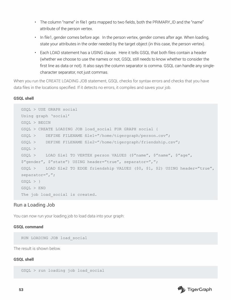
53
• The column “name” in file1 gets mapped to two fields, both the PRIMARY_ID and the “name”
attribute of the person vertex.
• In file1, gender comes before age. In the person vertex, gender comes after age. When loading,
state your attributes in the order needed by the target object (in this case, the person vertex).
• Each LOAD statement has a USING clause. Here it tells GSQL that both files contain a header
(whether we choose to use the names or not, GSQL still needs to know whether to consider the
first line as data or not). It also says the column separator is comma. GSQL can handle any single-
character separator, not just commas.
When you run the CREATE LOADING JOB statement, GSQL checks for syntax errors and checks that you have
data files in the locations specified. If it detects no errors, it compiles and saves your job.
GSQL shell
GSQL > USE GRAPH social
Using graph ‘social’
GSQL > BEGIN
GSQL > CREATE LOADING JOB load_social FOR GRAPH social {
GSQL > DEFINE FILENAME file1=”/home/tigergraph/person.csv”;
GSQL > DEFINE FILENAME file2=”/home/tigergraph/friendship.csv”;
GSQL >
GSQL > LOAD file1 TO VERTEX person VALUES ($”name”, $”name”, $”age”,
$”gender”, $”state”) USING header=”true”, separator=”,”;
GSQL > LOAD file2 TO EDGE friendship VALUES ($0, $1, $2) USING header=”true”,
separator=”,”;
GSQL > }
GSQL > END
The job load_social is created.
Run a Loading Job
You can now run your loading job to load data into your graph:
GSQL command
RUN LOADING JOB load_social
The result is shown below.
GSQL shell
GSQL > run loading job load_social

54
[Tip: Use “CTRL + C” to stop displaying the loading status update, then use
“SHOW LOADING STATUS jobid” to track the loading progress again]
[Tip: Manage loading jobs with “ABORT/RESUME LOADING JOB jobid”]
Starting the following job, i.e.
JobName: load_social, jobid: social_m1.1528095850854
Loading log: ‘/home/tigergraph/tigergraph/logs/restpp/restpp_loader_logs/
social/social_m1.1528095850854.log’
Job “social_m1.1528095850854” loading status
[FINISHED] m1 ( Finished: 2 / Total: 2 )
[LOADED]
+-----------------------------------------------------------------------+
| FILENAME | LOADED LINES | AVG SPEED | DURATION|
|/home/tigergraph/friendship.csv | 8 | 8 l/s | 1.00 s|
| /home/tigergraph/person.csv | 8 | 7 l/s | 1.00 s|
+-----------------------------------------------------------------------+
Notice the location of the loading log file. The example assumes that you installed TigerGraph in the default
location, /home/tigergraph/. In your installation folder is the main product folder, tigergraph. Within the tigergraph
folder are several subfolders, such as logs, document, config, bin, and gstore. If you installed in a different location,
say /usr/local/, then you would find the product folder at /usr/local/tigergraph.
Query Using Built-In SELECT Queries
You now have a graph with data! You can run some simple built-in queries to inspect the data.
Select Vertices
The following GSQL command reports the total number of person vertices. The person.csv data file had 7 lines
after the header.
GSQL command
SELECT count() FROM person
Similarly, the following GSQL command reports the total number of friendship edges. The friendship.csv file also
had 7 lines after the header.
GSQL command
SELECT count() FROM person-(friendship)->person

55
The results are illustrated below.
GSQL shell
GSQL > SELECT count() FROM person
[{
“count”: 7,
“v_type”: “person”
}]
GSQL > SELECT count() FROM person-(friendship)->person
[{
“count”: 14,
“e_type”: “friendship”
}]
GSQL >
Edge Count
Why are there 14 edges? For an undirected edge, GSQL actually creates two edges, one in each direction.
If you want to see the details about a particular set of vertices, you can use “SELECT *” and the WHERE clause to
specify a predicate condition. Here are some statements to try:
GSQL command
SELECT * FROM person WHERE primary_id==”Tom”
SELECT name FROM person WHERE state==”ca”
SELECT name, age FROM person WHERE age > 30
The result is in JSON format as shown below.
GSQL shell
GSQL > SELECT * FROM person WHERE primary_id==”Tom”
[{
“v_id”: “Tom”,
“attributes”: {
“gender”: “male”,
“name”: “Tom”,
“state”: “ca”,
“age”: 40
},

56
“v_type”: “person”
}]
GSQL > SELECT name FROM person WHERE state==”ca”
[
{
“v_id”: “Amily”,
“attributes”: {“name”: “Amily”},
“v_type”: “person”
},
{
“v_id”: “Tom”,
“attributes”: {“name”: “Tom”},
“v_type”: “person”
}
]
GSQL > SELECT name, age FROM person WHERE age > 30
[
{
“v_id”: “Tom”,
“attributes”: {
“name”: “Tom”,
“age”: 40
},
“v_type”: “person”
},
{
“v_id”: “Dan”,
“attributes”: {
“name”: “Dan”,
“age”: 34
},
“v_type”: “person”
}
]

57
Select Edges
In similar fashion, we can see details about edges. To describe an edge, you name the types of vertices and edges
in the three parts, with some added punctuation to represent the traversal direction:
GSQL syntax
source_type -(edge_type)-> target_type
Note that the arrow -> is always used, whether it’s an undirected or directed edge. That is because we are
describing the direction of the query’s traversal (search) through the graph, not the direction of the edge itself.
We can use the from_id predicate in the WHERE clause to select all friendship edges starting from the vertex
identified by the “from_id”. The keyword ANY to indicate that any edge type or any target vertex type is allowed.
The following two queries have the same result
GSQL command
SELECT * FROM person-(friendship)->person WHERE from_id ==”Tom”
SELECT * FROM person-(ANY)->ANY WHERE from_id ==”Tom”
Restrictions on built-in edge select queries
To prevent queries which might return an excessive number of output items, built-in edge queries have the
following restrictions:
1. The source vertex type must be specified.
2. The from_id condition must be specified.
There is no such restriction for user-defined queries.
The result is shown below.
GSQL
GSQL > SELECT * FROM person-(friendship)->person WHERE from_id ==”Tom”
[
{
“from_type”: “person”,
“to_type”: “person”,
“directed”: false,
“from_id”: “Tom”,
“to_id”: “Dan”,
“attributes”: {“connect_day”: “2017-06-03 00:00:00”},

58
“e_type”: “friendship”
},
{
“from_type”: “person”,
“to_type”: “person”,
“directed”: false,
“from_id”: “Tom”,
“to_id”: “Jenny”,
“attributes”: {“connect_day”: “2015-01-01 00:00:00”},
“e_type”: “friendship”
}
]
Another way to check the graph’s size is using one of the options of the administrator tool, gadmin. From a Linux
shell, enter the command
gadmin status graph -v
Linux shell
[tigergraph@localhost ~]$ gadmin status graph -v
verbose is ON
=== graph ===
[m1 ][GRAPH][MSG ] Graph was loaded (/usr/local/tigergraph/gstore/0/
part/): partition size is 4.00KiB, SchemaVersion: 0, VertexCount: 7,
NumOfSkippedVertices: 0, NumOfDeletedVertices: 0, EdgeCount: 14
[m1 ][GRAPH][INIT] True
[INFO ][GRAPH][MSG ] Above vertex and edge counts are for internal use
which show approximate topology size of the local graph partition. Use DML to
get the correct graph topology information
[SUMMARY][GRAPH] graph is ready
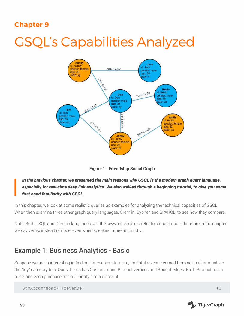
59
Chapter 9
GSQL’s Capabilities Analyzed
Figure 1 . Friendship Social Graph
In the previous chapter, we presented the main reasons why GSQL is the modern graph query language, especially for real-time deep link analytics. We also walked through a beginning tutorial, to give you some first hand familiarity with GSQL.
In this chapter, we look at some realistic queries as examples for analyzing the technical capacities of GSQL.
When then examine three other graph query languages, Gremlin, Cypher, and SPARQL, to see how they compare.
Note: Both GSQL and Gremlin languages use the keyword vertex to refer to a graph node, therefore in the chapter
we say vertex instead of node, even when speaking more abstractly.
Example 1: Business Analytics - Basic
Suppose we are in interesting in finding, for each customer c, the total revenue earned from sales of products in
the “toy” category to c. Our schema has Customer and Product vertices and Bought edges. Each Product has a
price, and each purchase has a quantity and a discount.
SumAccum<float> @revenue; #1
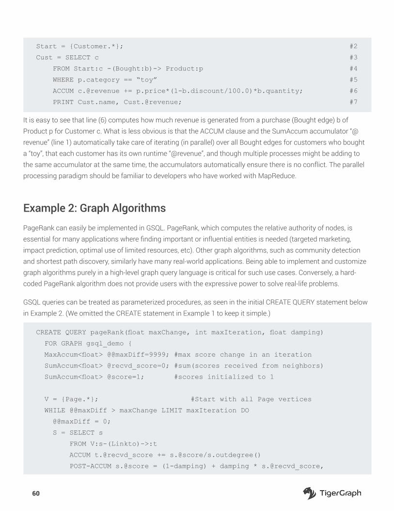
60
Start = {Customer.*}; #2
Cust = SELECT c #3
FROM Start:c -(Bought:b)-> Product:p #4
WHERE p.category == “toy” #5
ACCUM c.@revenue += p.price*(1-b.discount/100.0)*b.quantity; #6
PRINT Cust.name, Cust.@revenue; #7
It is easy to see that line (6) computes how much revenue is generated from a purchase (Bought edge) b of
Product p for Customer c. What is less obvious is that the ACCUM clause and the SumAccum accumulator “@
revenue” (line 1) automatically take care of iterating (in parallel) over all Bought edges for customers who bought
a “toy”, that each customer has its own runtime “@revenue”, and though multiple processes might be adding to
the same accumulator at the same time, the accumulators automatically ensure there is no conflict. The parallel
processing paradigm should be familiar to developers who have worked with MapReduce.
Example 2: Graph Algorithms
PageRank can easily be implemented in GSQL. PageRank, which computes the relative authority of nodes, is
essential for many applications where finding important or influential entities is needed (targeted marketing,
impact prediction, optimal use of limited resources, etc). Other graph algorithms, such as community detection
and shortest path discovery, similarly have many real-world applications. Being able to implement and customize
graph algorithms purely in a high-level graph query language is critical for such use cases. Conversely, a hard-
coded PageRank algorithm does not provide users with the expressive power to solve real-life problems.
GSQL queries can be treated as parameterized procedures, as seen in the initial CREATE QUERY statement below
in Example 2. (We omitted the CREATE statement in Example 1 to keep it simple.)
CREATE QUERY pageRank(float maxChange, int maxIteration, float damping)
FOR GRAPH gsql_demo {
MaxAccum<float> @@maxDiff=9999; #max score change in an iteration
SumAccum<float> @recvd_score=0; #sum(scores received from neighbors)
SumAccum<float> @score=1; #scores initialized to 1
V = {Page.*}; #Start with all Page vertices
WHILE @@maxDiff > maxChange LIMIT maxIteration DO
@@maxDiff = 0;
S = SELECT s
FROM V:s-(Linkto)->:t
ACCUM t.@recvd_score += s.@score/s.outdegree()
POST-ACCUM s.@score = (1-damping) + damping * s.@recvd_score,

61
s.@recvd_score = 0,
@@maxDiff += abs(s.@score - s.@score’);
END; #end while loop
PRINT V;
}#end query
Advanced Accumulation and Data Structures
So far, we have shown accumulators that aggregate numeric data into a single scalar result value. The expressive
power of GSQL is significantly enhanced by its support for complex-valued accumulators, which contain for
instance collections of tuples, possibly partitioned into groups, and optionally aggregated per group.
Example 3
We refine the revenue aggregation to show, for each customer c, the revenue by product category and the revenue by
discount.
GroupByAccum<string categ, SumAccum<float> revenue> @byCateg; #1
GroupByAccum<int disc, SumAccum<float> revenue> @byDiscount; #2
Start = {Customer.*}; #3
Cust = SELECT c #4
FROM Start:c -(Bought:b)-> Product:p #5
ACCUM c.@byCateg += (p.category->p.price*(1-
b.discount/100.0)*b.quantity), #6
c.@byDiscount += (b.discount->p.price*(1-
b.discount/100.0)*b.quantity); #7
Notice the declaration (in Line 1) of vertex accumulators called ‘byCategory’. These are group-by accumulators
that define the string attribute ‘categ’ as the group key and that associate to each group a sum accumulator called
‘revenue’, which is in charge of aggregating the group’s values.
Line (6) shows the syntax for writing the value p.price*(1-b.discount/100.0)*b.quantity into the ‘revenue’ sum
accumulator corresponding to the group of key p.category in the byCateg accumulator located at vertex c. A
similar group-by accumulator is defined in Line 2 to group sales by discount value, summing up the sales in
each group. To support the manipulation of accumulator values of collection type, GSQL also includes a foreach
primitive that iterates over the elements of the collection, binding a variable to them.

62
Multi-hop Traversals with Intermediate Result Flow
GSQL supports the specification of analytics that involve traversing multi-hop paths in the graph while
propagating intermediate results computed along the way. The following example illustrates how one can
concisely express a simple recommender system in GSQL.
Example 4
The following GSQL query generates a list of toy recommendations for customer 1. The recommendations are
ranked in the classical manner of recommender systems: each recommended toy’s rank is a weighted sum of the
likes by other customers. Each like by customer c is weighted by the similarity of c to customer 1. This similarity is
the standard log-cosine similarity, which reflects how many toys customers 1 and c already like in common. More
formally, for each customer c we define a vector likes_c of bits, such that bit i is set if and only if customer c likes
toy i. The log-cosine similarity measure between two customers x and y is defined as
lc(x, y) = log(1 + likes_x ʘ likes_y )
where ʘ denotes the dot product of two vectors. Note that likes_x ʘ likes_y simply counts the number of toys
liked in common by customers x and y. In the following, we assume that the fact that customer c likes product p is
modeled as a unique edge connecting c to p, labeled Likes.
SumAccum<float> @rank, @lc; #1
SumAccum<int> @inCommon; #2
Start = {Customer.1}; #3
ToysILike = #4
SELECT p #5
FROM Start:c -(Likes)-> Product:p #6
WHERE p.category == “toy”; #7
OthersWhoLikeThem = #8
SELECT o #9
FROM ToysILike:t <-(Likes)- Customer:o #10
WHERE o.id != 1 #11
ACCUM o.@inCommon += 1 #12
POST-ACCUM o.@lc = log (1 + o.@inCommon); #13
ToysTheyLike = #14
SELECT t #15
FROM OthersWhoLikeThem:o -(Likes)-> Product:t #16
WHERE t.category == “toy” #17
ACCUM t.@rank += o.@lc; #18
RecommendedToys = ToysTheyLike MINUS ToysILike; #19
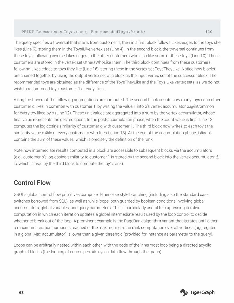
63
PRINT RecommendedToys.name, RecommendedToys.@rank; #20
The query specifies a traversal that starts from customer 1, then in a first block follows Likes edges to the toys she
likes (Line 6), storing them in the ToysILike vertex set (Line 4). In the second block, the traversal continues from
these toys, following inverse Likes edges to the other customers who also like some of these toys (Line 10). These
customers are stored in the vertex set OthersWhoLikeThem. The third block continues from these customers,
following Likes edges to toys they like (Line 16), storing these in the vertex set ToysTheyLike. Notice how blocks
are chained together by using the output vertex set of a block as the input vertex set of the successor block. The
recommended toys are obtained as the difference of the ToysTheyLike and the ToysILike vertex sets, as we do not
wish to recommend toys customer 1 already likes.
Along the traversal, the following aggregations are computed. The second block counts how many toys each other
customer o likes in common with customer 1, by writing the value 1 into o’s vertex accumulator o.@inCommon
for every toy liked by o (Line 12). These unit values are aggregated into a sum by the vertex accumulator, whose
final value represents the desired count. In the post-accumulation phase, when the count value is final, Line 13
computes the log-cosine similarity of customer o with customer 1. The third block now writes to each toy t the
similarity value o.@lc of every customer o who likes t (Line 18). At the end of the accumulation phase, t.@rank
contains the sum of these values, which is precisely the definition of the rank.
Note how intermediate results computed in a block are accessible to subsequent blocks via the accumulators
(e.g., customer o’s log-cosine similarity to customer 1 is stored by the second block into the vertex accumulator @
lc, which is read by the third block to compute the toy’s rank).
Control Flow
GSQL’s global control flow primitives comprise if-then-else style branching (including also the standard case
switches borrowed from SQL), as well as while loops, both guarded by boolean conditions involving global
accumulators, global variables, and query parameters. This is particularly useful for expressing iterative
computation in which each iteration updates a global intermediate result used by the loop control to decide
whether to break out of the loop. A prominent example is the PageRank algorithm variant that iterates until either
a maximum iteration number is reached or the maximum error in rank computation over all vertices (aggregated
in a global Max accumulator) is lower than a given threshold (provided for instance as parameter to the query).
Loops can be arbitrarily nested within each other, with the code of the innermost loop being a directed acyclic
graph of blocks (the looping of course permits cyclic data flow through the graph).

64
Query Calling Query
GSQL supports queries calling named, parameterized queries. GSQL supports vertex-, edge- as well as attribute-
level modifications (insertions, deletions and updates), with a syntax inspired by SQL.
Turing Completeness
As previously stated, GSQL is Turing-complete. This is clear when you obverse GSQL’s support for conditional
branching, looping, and storage variables.
GSQL Compared to Other Graph Languages
GSQL can be compared to other prominent graph query languages in circulation today. This comparison seeks
to transcend the particular syntax or the particular way in which semantics are defined, focusing on expressive
power classified along the following key dimensions.
1. Accumulation: What is the language support for the storage of (collected or aggregated) data computed by
the query?
2. Multi-hop Path Traversal: Does the language support the chaining of multiple traversal steps into paths,
with data collected along these steps?
3. Intermediate Result Flow: Does the language support the flow of intermediate results along the steps of the
traversal?
4. Control Flow: What control flow primitives are supported?
5. Query-Calling-Query: What is the support for queries invoking other queries?
6. SQL Completeness: Is the language SQL-complete? That is, is it the case that for a graph-based
representation G of any relational database D, any SQL query over D can be expressed by a GSQL query
over G?
7. Turing completeness: Is the language Turing-complete?
Gremlin
Gremlin is a graph query language that specifies graph analytics as pipelines of operations through which objects
(called “traversers”) flow, evolving and collecting information along the way. Operations can for instance replace
(within the traverser) a vertex with its in- or out-neighbor, its in- or out-edge, its attribute, etc., while also extending
the traverser with bindings of variables to values computed from the contents of the traverser. The semantics of
Gremlin is specified operationally, in functional programming style.

65
Gremlin is a Turing-complete language and as such as expressive as GSQL. We detail below how it covers the
expressivity dimensions we articulated, referring to the Apache TinkerPop3 v3.2.7 documentation.
1. Accumulation
Gremlin supports the collection of data (into lists or tables), as well as their aggregation using either user-
defined aggregation functions or the usual SQL built-in aggregates. Group-by aggregation is supported as in
SQL, by defining a relational table, specifying its grouping attributes and aggregated columns.
• Gremlin inherits a limitation from SQL: like SQL queries, Gremlin queries can group a table by one
group-by attribute list or by another, but not simultaneously by both. Achieving two different group-
by aggregations of the same collected data would require a verbose query that defines the same
table of variable bindings twice, grouping each table accordingly. Contrast this with the ease with
which GSQL specifies the simultaneous computation of the two groupings of the same data by
simply writing each value into two distinct grouping accumulators.
• Intermediate results computed during the traversal can be stored either in global variables via the
“sideeffect” operator (akin to GSQL’s global accumulators) or into attributes (aka properties) of
vertices/edges.
2. Multi-hop Path Traversal
Gremlin’s design was motivated by the desire to concisely specify multi-hop linear paths as a pipeline of
individual traversal step operations.
3. Intermediate Result Flow
Intermediate results can be transmitted down the pipeline by storage into the traverser object via a variable
binding (in the same spirit in which GSQL passes data via accumulators).
4. Control Flow
Gremlin features both if-then-else style branching and loops, whose guard conditions do not only specify
global intermediate results but also data local to the traversers.
5. Query-Calling-Query
This is supported as Gremlin allows users to define functions that can invoke each other, including
recursively.
6. SQL and Turing Completeness
Gremlin is Turing-complete and thus SQL-complete.
Programming Style
A characteristic of Gremlin is that the attributes (properties) of vertices and edges are modeled as a property
graph that needs to be navigated in order to reach the values of properties. To access several attributes, one
needs to perform branching navigation in the property graph (from a given vertex or edge, we need to follow one
navigation branch to each of its attribute values).
Another characteristic is that its syntax was optimized to concisely express linear (non-branching) path

66
navigation. Branching navigation is achieved in a verbose way, by binding a variable to the vertex at the
branching point, following the side branch in another linear navigation, then jumping back to the branching point
to resume following the main branch.
The interaction of these two characteristics leads to convoluted navigation and verbose query expressions
in queries that need to simultaneously access various attributes of the same edge/vertex. We illustrate by
translating Example 1 to Gremlin.
toys =
V().hasLabel(‘Customer’).as(‘c’) (1)
.values(‘name’).as(‘name’) (2)
.outE(‘Bought’).as(‘b’) (3)
.values(‘discount’).as(‘disc’) (4)
.select(‘b’) (5)
.values(‘quantity’).as(‘quant’) (6)
.select(‘b’) (7)
.outV() (8)
.has(‘Product’, ‘category’, eq(‘toy’)) (9)
.as(‘p’) (10)
.values(‘price’).as(‘price’) (11)
.select(‘price’, ‘disc’, ‘quant’) (12)
.map{it.get().price*(1-it.get().disc/100.0)*it.get().quant} (13)
.as(‘sale_price’) (14)
.select(‘name’,’sale_price’) (15)
.group().by(‘name’).by(sum()) (16)
The above program performs the following steps. (1) Check that the vertex has label ‘Customer’, if so bind variable
‘c’ to it. (2) Go to its ‘name’ attribute, bind variable ‘name’ to it. (3) Go to outgoing ‘Bought’ edge, bind variable ‘b’
to it. (4) Go to value of ‘discount’ property of ‘b’, bind variable ‘disc’. (5) Go back to edge ‘b’. (6) Go to value of b’s
property ‘quantity’, bind variable ‘quant’. (7) Go back to edge ‘b’. (8) Go to target vertex of edge ‘b’. (9) Check that
it has label ‘Product’, and a property ‘category’ whose value is ‘toy’. (10) Bind variable ‘p’ to this ‘Product’ vertex.
(11) Go to the value of the ‘price’ property, bind variable ‘price’ to it. (12) Output tuples of variable bindings with
components for the variables ‘price’, ‘disc’, and ‘quant’. (13) For each such tuple, referred to by the built-in variable
‘it’, compute the price per sale by executing the function given as argument to the map. (14) Bind variable ‘sale_
price’ to the value computed at step 13. (15) Output tuples of variable bindings with components for the variables
‘name’ and ‘sales_price’. (16) Group these tuples by ‘name’, summing up the ‘sales_price’ column.
Note that the navigation to the values of the ‘price’, ‘discount’, and ‘quantity’ attributes is branching and involves
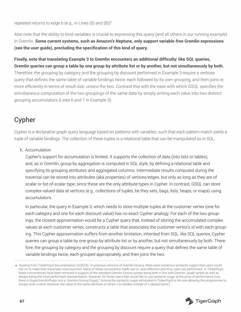
67
repeated returns to edge b (e.g., in Lines (6) and (8))4.
Also note that the ability to bind variables is crucial to expressing this query (and all others in our running example)
in Gremlin. Some current systems, such as Amazon’s Neptune, only support variable-free Gremlin expressions
(see the user guide), precluding the specification of this kind of query.
Finally, note that translating Example 3 to Gremlin encounters an additional difficulty: like SQL queries,
Gremlin queries can group a table by one group-by attribute list or by another, but not simultaneously by both.
Therefore, the grouping by category and the grouping by discount performed in Example 3 require a verbose
query that defines the same table of variable bindings twice, each followed by its own grouping, and then joins or,
more efficiently in terms of result size, unions the two. Contrast this with the ease with which GSQL specifies the
simultaneous computation of the two groupings of the same data by simply writing each value into two distinct
grouping accumulators (Lines 6 and 7 in Example 3).
Cypher
Cypher is a declarative graph query language based on patterns with variables, such that each pattern match yields a
tuple of variable bindings. The collection of these tuples is a relational table that can be manipulated as in SQL.
1. Accumulation
Cypher’s support for accumulation is limited. It supports the collection of data (into lists or tables),
and, as in Gremlin, group-by aggregation is computed in SQL style, by defining a relational table and
specifying its grouping attributes and aggregated columns. Intermediate results computed during the
traversal can be stored into attributes (aka properties) of vertices/edges, but only as long as they are of
scalar or list-of-scalar type, since these are the only attribute types in Cypher. In contrast, GSQL can store
complex-valued data at vertices (e.g., collections of tuples, be they sets, bags, lists, heaps, or maps) using
accumulators.
In particular, the query in Example 3, which needs to store multiple tuples at the customer vertex (one for
each category and one for each discount value) has no exact Cypher analogy. For each of the two group-
ings, the closest approximation would be a Cypher query that, instead of storing the accumulated complex
values at each customer vertex, constructs a table that associates the customer vertex’s id with each group-
ing. This Cypher approximation suffers from another limitation, inherited from SQL: like SQL queries, Cypher
queries can group a table by one group-by attribute list or by another, but not simultaneously by both. There-
fore, the grouping by category and the grouping by discount require a query that defines the same table of
variable bindings twice, each grouped appropriately, and then joins the two:
4 Quoting from TinkerPop3 documentation (3/2018): “In previous versions of Gremlin-Groovy, there were numerous syntactic sugars that users could rely on to make their traversals more succinct. Many of these conventions made use of Java reflection and thus, were not performant. In TinkerPop3, these conveniences have been removed in support of the standard Gremlin-Groovy syntax being both in line with Gremlin-Java8 syntax as well as always being the most performant representation. However, for those users that would like to use syntactic sugar at the price of performance loss, there is SugarGremlinPlugin (a.k.a. Gremlin-Groovy-Sugar).” Among the syntactic sugar eliminated in TinkerPop3 is the one allowing the programmer to simply write v.name wherever the value of the name attribute of vertex v is needed, instead of v.values(’name’).

68
MATCH (c:Customer) -[b:Bought]-> (p:Product)
WITH c, p.category as cat,
sum(p.price*(1-b.discount/100.0)*b.quantity) as rev
WITH c, collect({category:cat, revenue:rev}) as byCateg
MATCH (c) -[b:Bought]-> (p:Product)
WITH c, byCateg, b.discount as disc,
sum(p.price*(1-b.discount/100.0)*b.quantity) as rev
RETURN c, byCateg, collect({discount:disc, revenue:rev}) as byDisc
Contrast this with the ease with which GSQL simultaneously computes the two groupings of the same data
by simply writing each value into two distinct grouping accumulators. Note that towards efficient evaluation,
Cypher’s optimizer would have to identify the fact that the two MATCH clauses can reuse matches, instead
of redundantly recomputing them.
2. Multi-hop Path Traversal
Cypher can specify multi-hop patterns with variables.
3. Intermediate Result Flow
Intermediate results can be accessed along the traversal path by referring to the variables bound to them.
4. Control Flow
Cypher’s control flow includes if-then-else style branching. Loop control is limited, supporting only loops
over lists of elements computed prior to the iteration’s start. This can be used to simulate loops of given
number of iterations, by first creating a corresponding list of integers: unwind range(1,30) as iter specifies a
30-iteration loop with iteration variable iter and unwind L as e specifies an iteration over the elements of the
list L, binding variable e to each.
Recalling the PageRank version that iterates until the maximum error falls below a threshold, note that it
relies on loops whose guard condition depends on an intermediate result updated during the iteration. This
kind of loop is not supported in Cypher and the corresponding class of algorithms is not expressible (e.g.,
PageRank is provided as built-in primitive implemented in Java).
5. Query-Calling-Query
Cypher allows users to define functions but these must be implemented in Java, as per the Neo4j developer
manual. This design introduces two drawbacks. First, the programmer must be fluent in both Cypher and
Java simultaneously. Second, user-defined functions are black boxes to the neo4j optimizer and therefore
cannot be optimized in the context of the calling query.
6. SQL and Turing Completeness
Cypher is SQL-complete but not Turing-complete. The loop control limitations mentioned above are one
of the reasons precluding Turing completeness. This statement ignores arbitrary user-defined functions,
whose implementation in Java is allowed by Neo4j, and in whose presence the question becomes

69
meaningless since Java is Turing-complete.
SPARQL
SPARQL is a declarative query language designed for semantic-graph data where connected data is represented
in the Resource Description Framework (RDF https://www.w3.org/RDF/) format. The primary goal of RDF was to
make web pages machine digestible. SPARQL was to enable higher-level querying of the semantic web. Over the
time, RDF and SPARQL have been extended to manage a wider range of interconnected data. That being said,
SPARQL was not designed for the property graph model (node entities and edge entities, each with characteristic
attributes).
RDF defines data in terms of triples: <subject><predicate><object>. One triple describes the relationship between
two entities or the relationship between an entity and one of its attributes. Each triple can be thought of as an
edge in a graph: <source_vertex><edge><target_vertex>, thus an RDF dataset is a graph. Consider the following
triple: <John Smith><teacherOf><Calculus>. “John Smith” and “Calculus” are the subject and object, respectively.
“teacherOf” is the predicate indicating their relationship. Consider another triple <John Smith><gender><Male>.
“John Smith” is the subject, and “Male” is his attribute. The predicate “gender” describes the relationship between
the subject and its attribute.
SPARQL syntax borrows many keyword and design philosophies from SQL. For example,
SELECT ?title
WHERE
{
<http://example.org/book/book1> <http://purl.org/dc/elements/1.1/title>
?title .
}
Just as in SQL, SELECT projects a set of expressions from the underlying data set (triple store). The WHERE
clause holds a list of graph patterns in triple or path format. The user may use ? or $ in the subject or the object
position to ask for matches and to bind variables to those positions.
1. Accumulation
SPARQL has aggregation operators COUNT, SUM, etc. and a GROUP BY clause as found in SQL. A query
can select a select of triples and then aggregate them. One approach is to define a named graph to store
intermediate results. This is similar to Cypher’s WITH clause and VIEW concept in SQL. Then, the user can
select from the named graph in the FROM clause. The limitations and differences from GSQL are the same
as the discussion in Cypher. Example:
CREATE GRAPH <urn:example/g/g1>
INSERT {
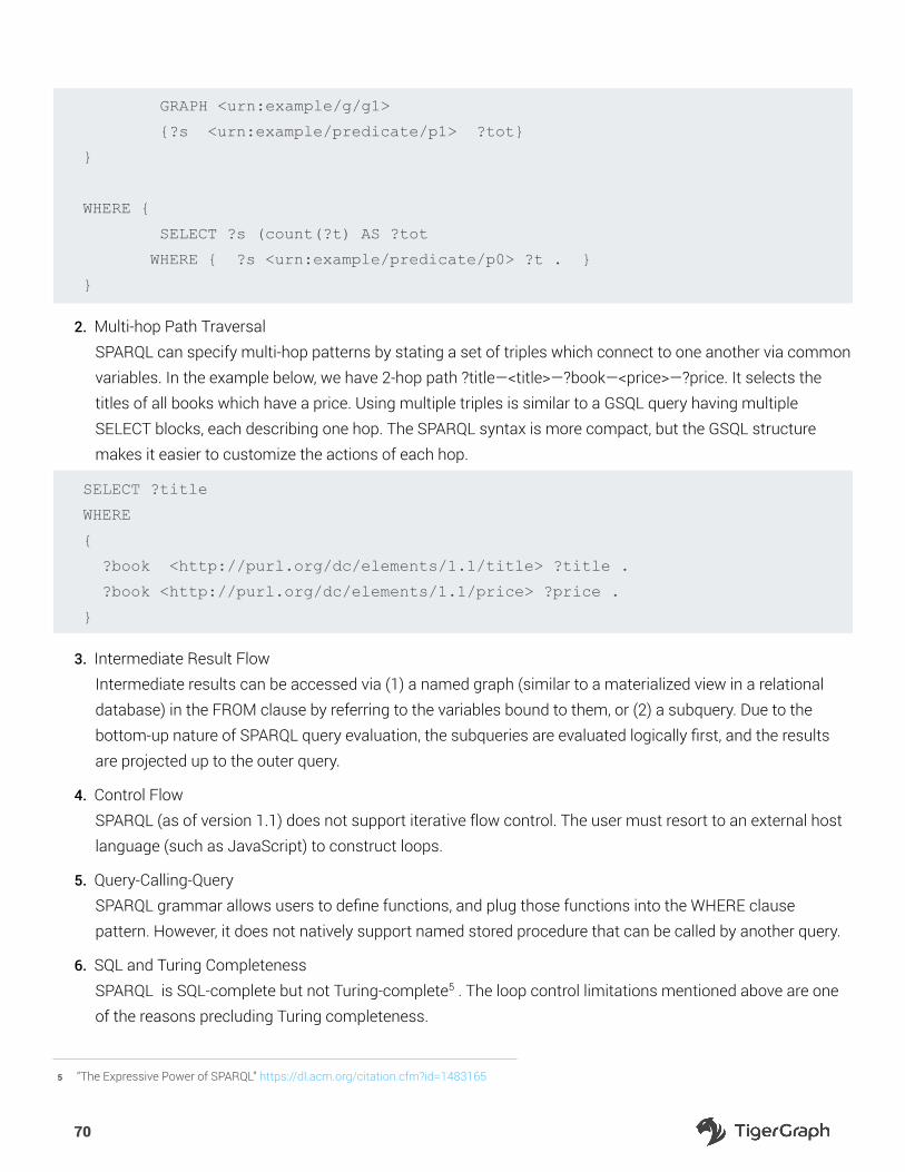
70
GRAPH <urn:example/g/g1>
{?s <urn:example/predicate/p1> ?tot}
}
WHERE {
SELECT ?s (count(?t) AS ?tot
WHERE { ?s <urn:example/predicate/p0> ?t . }
}
2. Multi-hop Path Traversal
SPARQL can specify multi-hop patterns by stating a set of triples which connect to one another via common
variables. In the example below, we have 2-hop path ?title—<title>—?book—<price>—?price. It selects the
titles of all books which have a price. Using multiple triples is similar to a GSQL query having multiple
SELECT blocks, each describing one hop. The SPARQL syntax is more compact, but the GSQL structure
makes it easier to customize the actions of each hop.
SELECT ?title
WHERE
{
?book <http://purl.org/dc/elements/1.1/title> ?title .
?book <http://purl.org/dc/elements/1.1/price> ?price .
}
3. Intermediate Result Flow
Intermediate results can be accessed via (1) a named graph (similar to a materialized view in a relational
database) in the FROM clause by referring to the variables bound to them, or (2) a subquery. Due to the
bottom-up nature of SPARQL query evaluation, the subqueries are evaluated logically first, and the results
are projected up to the outer query.
4. Control Flow
SPARQL (as of version 1.1) does not support iterative flow control. The user must resort to an external host
language (such as JavaScript) to construct loops.
5. Query-Calling-Query
SPARQL grammar allows users to define functions, and plug those functions into the WHERE clause
pattern. However, it does not natively support named stored procedure that can be called by another query.
6. SQL and Turing Completeness
SPARQL is SQL-complete but not Turing-complete5 . The loop control limitations mentioned above are one
of the reasons precluding Turing completeness.
5 “The Expressive Power of SPARQL” https://dl.acm.org/citation.cfm?id=1483165

71
Final Remarks
There is one more feature of GSQL that sets it apart from other graph query languages, which enables better query
optimization as well as added security.
GSQL assumes a predefined schema, which is stored as metadata in the database catalog. This improves
storage and access efficiency, because the schema metadata can be factored out of the vertex/edge/attribute
representation. This leads to increased performance not only due to space savings but also because queries
can be optimized to a greater degree when a deeper understanding of the data model is known in advance: more
filtering, better ordering, more shortcuts, etc. Exploiting pre-defined schemas at optimization time is a tried-and-
true database technique that has time and again led to better performance.
Additionally, the pre-defined schema is exploited for security and privacy purposes to provide graph schema-
aware access control. GSQL’s MultiGraph feature allows an unlimited number of subgraph schemas to be defined
within the global schema, and then it enhances traditional role-based access control by using subgraph name
as an additional factor for granting privileges. This functionality is critical in real-life applications as it enables
multiple tenants (e.g., multiple departments of a company) to use the same graph database with distinct access
permissions. This is the industry’s first and only such support so far.
GSQL matches or surpasses the expressive power of other graph query languages. While the underlying
programming paradigm is a matter of taste, GSQL has been designed for compatibility with both SQL and NoSQL’s
Map-Reduce programming paradigm, thus appealing to both programmer communities.

72
Chapter 10
Real-Time Deep Link Analytics in the Real World
As the first and only native parallel graph database with real-time deep link analytics capability, TigerGraph is uniquely qualified to solve some of today’s business challenges. In this chapter, we examine several real-world use cases and show how real-time deep link analytics is now providing real solutions and real business value.
Combating Fraud and Money Laundering with Graph Analytics
Dirty money and money laundering have been around since the existence of currency itself. On a global level, as
much as $2 billion is washed annually, estimates the United Nations6 . Today’s criminals are sophisticated, using
ever-adapting tactics to bypass traditional anti-fraud solutions. Even in cases where enterprises do have enough
data to reveal illicit activity, more often than not they are unable to conduct analysis to uncover it.
6 https://www.unodc.org/unodc/en/money-laundering/globalization.html

73
As the fight against money laundering continues, AML (anti money laundering) compliance has become big
business. Global spending in AML alone weighs in at more than $8 billion, says WealthInsight7 . This figure will
continue to grow, considering how any organization facilitating financial transactions also falls within the scope of
AML legislation.
But combating crime is never easy. Especially when organizations face pressing needs for cost reduction
and faster time to AML compliance in order to avoid regulatory fees. Legacy monitoring systems have proven
burdensome and expensive to tune, validate and maintain. Often involving manual processes, they are generally
incapable of analyzing massive volumes of customer, institution, and transaction data. Yet it is this type of data
analysis that is so critical to AML success.
New ideas have emerged to tackle the AML challenge. These include semi-supervised learning methods, deep
learning based approaches, and network/graph based solutions. Such approaches must be able to work in real
time and handle large data volumes – especially as new data are generated 24/7. That’s why a holistic data
strategy is best for combating financial crime, particularly with machine learning (ML) and AI to help link and
analyze data connections.
Graph Analytics for AML
Graph analytics has emerged at the forefront as an ideal technology to support AML. Graphs overcome the
challenge of uncovering the relationships in massive, complex, and interconnected data. The graph model is
designed from the ground up to treat relationships as first-class citizens. This provides a structure that natively
embraces and maps data relationships, even in high volumes of highly connected data. Conducted over such
interconnected data, graph analytics provides maximum insight into data connections and relationships.
For example, “Degree Centrality” provides the number of links going in or out of each entity. This metric gives a
count of how many direct connections each entity has to other entities within the network. This is particularly
helpful for finding the most connected accounts or entities which are likely acting as a hub, and connecting to a
wider network.
Another is “Betweenness,” which gives the number of times an entity falls on the shortest path between other
entities. This metric shows which entity acts as a bridge between other entities. Betweenness can be the starting
point to detect any money laundering or suspicious activities.
Today’s organizations need real-time graph analytic capabilities that can explore, discover, and predict very
complex relationships. This represents Real-Time Deep Link Analytics, achieved utilizing three to 10+ hops of
traversal across a big graph, along with fast graph traversal speed and data updates.
Let’s take a look at how Real-Time Deep Link Analytics combats financial crime by identifying high-risk
transactions. We’ll start with an incoming credit card transaction, and demonstrate how this transaction is
7 https://www.marketresearch.com/product/sample-7717318.pdf

74
related to other entities can be identified:
New Transaction → Credit Card → Cardholder → (other) Credit Cards → (other)
Bad Transactions
This query uses four hops to find connections only one card away from the incoming transaction. Today’s
fraudsters try to disguise their activity by having circuitous connections between themselves and known bad
activity or bad actors. Any individual connecting the path can appear innocent, but if multiple paths from A to B
can be found, the likelihood of fraud increases.
Given this, successful anti-money laundering requires the ability to traverse several hops. This traversal pattern
applies to many other use cases – where you can simply replace the transaction with a web click event, a phone
call record, or a money transfer. With Real-Time Deep Link Analytics, multiple, hidden connections are uncovered
and fraud is minimized.
By linking data together, Real-Time Deep Link Analytics can support rules-based ML methods in real time to
automate AML processes and reduce false positives. Using a graph engine to incorporate sophisticated data
science techniques such as automated data flow analysis, social network analysis, and ML in their AML process,
enterprises can improve money laundering detection rates with better data, faster. They can also move away from
cumbersome transactional processes, and towards a more strategic and efficient AML approach.
Example: E-payment Company
For one example of graph analytics powering AML, we can look towards the #1 e-payment company in the world.
Currently this organization has more than 100 million daily active users, and uses graph analytics to modernize its
investigation methods.
Previously, the company’s AML practice was a very manual effort, as investigators were involved with everything
from examining data to identifying suspicious money movement behavior. Operating expenses were high and the
process was highly error-prone.
Implementing a graph analytics platform, the company was able to automate development of intelligent AML
queries, using a real-time response feed leveraging ML. Results included a high economic return using a more
effective AML process, reducing false positives and translating into higher detection rates.
Example: Credit Card Company
Similarly, a top five payment provider sought to improve its AML capabilities. Key pain points include high cost
and inability to comply with federal AML regulations – resulting in penalties. The organization relied on a manual
investigative process performed by a ML team comprised of hundreds of investigators, resulting in a slow, costly
and inefficient process with more than 90 percent false positives.
The company currently is leveraging a graph engine to modernize its investigative process. It has moved from

75
having its ML team cobble processes together towards combining the power of graph analytics with ML to provide
insight into connections between individuals, accounts, companies and locations.
By uniting more dimensions of its data, and integrating additional points – such as external information about
customers – it is able to automatically monitor for potential money laundering in real time, freeing up investigators
to make more strategic use of their now-richer data. The result is a holistic and insightful look at its colossal
amounts of data, producing fewer false positive alerts.
As we continue into an era of data explosion, it is more and more important for organizations to make the most in
analyzing their colossal amounts of data in real time for AML. Graph analytics offers overwhelming potential for
organizations in terms of cost reduction, in faster time to AML compliance and most importantly, in their ability to
stop money laundering fraudsters in their tracks.
How Graph Analytics Is Powering E-commerce
We have entered an era where e-Commerce rules retail. Consider how reports project online sales to hit more than
$4 trillion by 2020, representing 14.6% of total retail spending worldwide (source: eMarketer8) . Over the past few
years, online shopping has transformed how we buy, bringing in a new “Age of the Consumer.” Today, shoppers
have access to more information than ever around products and brands, all informing their purchasing decisions.
They also are taking the lead in their own online shopping experiences, with the global marketplace available at
their fingertips.
8 https://www.emarketer.com/Article/Worldwide-Retail-Ecommerce-Sales-Will-Reach-1915-Trillion-This-Year/1014369

76
In turn, e-Commerce has embraced AI-powered assistants, recommendation engines, and even automated
platforms to help consumers consider what to evaluate and buy. Insights generated from AI platforms provide
tremendous value, and can potentially drive further revenues for companies, as well as provide shoppers with a
better, more customized customer experience.
Traditional brick-and-mortar sales relied, and continue to rely, on establishing a connection with the customer
in the form of discerning and evaluating their needs, making recommendations and walking them through the
sales process. Connections matter even more so when it comes to online sales, as the most successful retailers
today offer a customer-centric e-Commerce platform. This involves a consistent multipath purchase experience,
achieved through a 360-degree view of each and every customer. Being able to translate customer data and
activity into actionable intelligence to support the customer during their shopping experience with product
recommendations and more can lead to increased conversions and higher units per transaction.
The key to successfully leveraging this data is having it and being able to analyze it effectively in the first place, not
to mention being able to do so in real time, during a customer’s live shopping session. Most e-Commerce retailers
are able to gather the data, but are finding that traditional analytic solutions are missing the mark to achieve this.
Historically, solutions have been too slow or expensive, and often are incapable of deriving sophisticated insight
from massive amounts of customer, transaction, and external data.
Real-time offers — be it products on hand, conditional promotions or free shipping to save a sale — require
knowing your customers, and knowing them well. This means e-Commerce sites need to collect and leverage
consumer segmentation data as quickly as possible to provide targeted recommendations and customer service.
The result is being able to offer a more personalized shopping experience that customers enjoy, engage with, and
consistently come back to for their needs.
Delivering a Better Online Shopping Experience...And Driving Revenue
Achieving this is no easy feat, especially using traditional databases that tend to store data in tables. That’s why
more and more retailers are turning to the power of graph database technology to support real-time analytics
and more. For retail, graph databases are the ideal choice for an industry where connections are of the utmost
essence. This is because graph databases are designed from the ground up to treat relationships as first-class
citizens, providing a structure natively embracing the relationships between data. This ensures better storing,
processing and querying of connections than ever before.
For example, consider a simple personalized recommendation such as “customers who liked what you liked also
bought these items.” Starting from a person, a query made in a graph database first identifies items viewed/liked/
bought. Second, it finds other people who have viewed/liked/bought those items. Third, it identifies additional
items bought by those people.
Person → Product → (other)Persons → (other) Products

77
To power such queries, over the past few years graph databases have seen a major uptick in enterprise adoption,
particularly by retailers powering e-Commerce sites. While the first generation of graph database solutions have
been helpful in addressing the e-Commerce data problem, they are not without their limitations. Query speeds and
analysis of data are relatively slow, with graph engines only able to support traversals (the process of visiting, or
checking and/or updating, points of data) to a certain extent. Deeper traversals allow you to glean better insights
from data.
Empowering E-Commerce with Real-Time Deep Link Analytics
Recently, we have seen the next phase in the graph database evolution, with technology fulfilling the needs of
e-Commerce by providing Deep Link Analytics. This enables customer intelligence in real time, along with powerful
relationship analysis. With these real-time capabilities, e-Commerce sites can quickly synthesize and make sense
of customer behavior. The result is the capture of key Business Moments, transient opportunities where people,
businesses, data, and “things” work together dynamically to create value used to personalize the customer
experience, which leads to more transactions.
This is accomplished as new graph database technology supports 10+ hops (or traversals of data points
as described above), unlike being limited to just two as first-generation solutions are. Each hop adds more
intelligence about an individual user’s shopping history — whether it is their first visit or they are a repeat
customer. Analyzing the data/product/customer location/weather based on location/recommended products
requires the capability to traverse the data to present a recommendation in real time.
The query above requires three hops in real time, so it is beyond the two-hop limitation of current-generation graph
technology on larger data sets. Adding in another relationship easily extends the query to four or more hops.
This data continuously feeds the AI and machine learning algorithms designed to bring a better online shopping
experience.
Deep Link Analytics allow e-Commerce companies to be able to traverse these data, creating smarter AI and
machine learning to deliver competitive advantages, close more deals, and build customer loyalty. It all comes
down to being able to derive better insight by considering more connections among your data to adequately
address a shopper’s online behavior and preferences.
Deep Link Analytics for Product Recommendations
Example: Mobile E-Commerce Company
Let’s consider an example of Deep Link Analytics being used by a retailer today. A major global e-Commerce
platform uses Deep Link Analytics to model its vast product catalog, map its consumer entity data, and to perform
real-time analytics over its complex and colossal amounts of data. This leads to real-time recommendations that

78
are personalized for each shopper, driving sales and revenue.
At a technical level, the solution has increased query speeds by 100x compared to the company’s previous in-
house solution, with query responses in under 100 milliseconds. It also has saved memory usage by 10x, achieved
through efficient graph-based encoding and compression. As fewer machines are needed, this also has helped cut
hardware management and maintenance costs.
Data scientists and machine learning experts are able to do more, faster, as they are able to use a single massive
graph integrating all the company’s connected data. The business derives insight from its massive amounts of
data to support better decision making and improving time to market. The graph database platform also provides
the speed and scalability needed to make the most data relationships for competitive advantage.
The Customer Connection
Retailers are finding that connecting with consumers online is just as important as connecting with them in
person when they shop in a brick-and-mortar location. To achieve this, it has become more and more relevant for
e-Commerce to find ways to scan through huge amounts of data and to make sense of it.
Today, it’s more possible to do this than ever before, especially using a graph database where connections among
data are at the forefront. As graph databases mature, they are powering deeper insight by supporting queries over
more connected data. Customers enjoy a better shopping experience, while retailers benefit from happier and
more engaged shoppers along with additional sales and revenues.
Electric Power System Modernization
Creating a faster-than-real-time Energy Management System (EMS) is a huge challenge for the power industry.
Faster-than-real-time means the EMS must be capable of completing execution within a Supervisory control and
data acquisition (SCADA) sample cycle, typically 5 seconds.
Faster-than-real-time EMS capability is key to maintaining awareness over power system events, helping prevent
power system blackouts from occurring. For over a decade, power system engineers have been unsuccessful at
developing faster EMS applications for large-scale power systems. If achieved, it would help operators in control
centers to make power system operations more secure and cost-effective. So far, no commercial EMS had been
able to perform at such faster-than-real-time levels.
Technical challenges to curb EMS application computation efficiency include: A) The power system becoming
larger and larger to meet growing demand, B) High renewable energy penetration, FACTS devices, and HVDC
transmission lines making power system models more complex, and C) Rapid fluctuations in power demand and
supply combined with fast-response devices leading to more frequent and intensive recalculations.

79
Parallel computing is a breakthrough solution for speeding up EMS applications. Power system engineers have
investigated different parallel computing approaches based on relational database structure to improve the EMS
application computing efficiency, but until now have been unable to achieve faster-than-real-time EMS.
Example: National Utility Company
Using TigerGraph’s native parallel graph database, with node-as-a-compute-engine design, State Grid Corporation
of China (SGCC) has achieved a faster-than-real-time EMS prototype, verified by provincial power system cases.
Conventionally, power systems are modeled using relational databases in a collection of interlinked tables. As
different components of power systems are stored in separate tables, they need to be linked together using
shared key values to model the connectivity and topology of the power system. Connecting or linking across
separate tables (database joins) takes about 25% of the total processing time for power flow calculation and 35%
for power grid state estimation, according to the results of the case study.
The standard approach of solving large-scale linear equations requires bulky, time-intensive matrix operations.
Modeling a power system as a graph (instead of a matrix) represents connections and topology more naturally.
No data preparation is needed, cutting 25-35% of the generally required time for power flow calculation and
state estimation. Bus ordering and admittance graph formation are performed in nodal parallel (with all nodes
computing at the same time to ensure the ordering sequence and admittance graph are in parallel). Symbolic
and numerical factorization and forward/backward substitution are performed in hierarchical parallel, with nodes
partitioned into levels. Nodes at the same level are calculated in parallel, starting with the lowest level. Core
calculations are all conducted on graph, and solved values are stored as attributes of vertices and edges of the
graph - rather than unknown variables in the vector or matrix.
In the conventional approach, power system problems are solved as unknown variables and assigned to the X
vector. To visualize the solved value, a mapping process is used to link the unknown variable to displays.
Using TigerGraph, solved values are stored as attributes of vertices and edges on a graph — forgoing the need
for a mapping process. According to the test case, output visualization takes about 70% of total time for power
flow calculation, and 28% for state estimation when using the conventional approach. Using TigerGraph graph
database and graph computing, that portion of the time is eliminated.
This table summarizes test results of the faster-than-real-time EMS comparing with D5000, the widely used
commercial EMS covering most control centers in China and many other countries.

80
The total execution time of the three major EMS applications — State Estimation, Power Flow, and Contingency
Analysis — is a little above 1 second combined, which is much less than the SCADA sample cycle standard of 5
seconds. With the help of TigerGraph, State Grid of China has achieved the first viable faster-than-real-time EMS
solution for commercial use.
Faster than real-time Energy Management System (EMS) has been the holy grail for power management
especially as any power outages directly affect the productivity and economic output / GDP (Gross Domestic
Product) of the nation. Such a system can identify mismatches between power demand and supply, lower power
consumption for non-critical parts of the grid, and divert power to higher priority areas for industrial output and
national security and be able to accomplish all of this in under one second.
Test on a Real Provincial 2650 Bus System
Test System State Estimation Power Flow Contingency Analysis
Commercial EMS 4488 ms 3817 ms 18000 ms
TigerGraph Based EMS Prototype 172 ms 79 ms 772 ms

81
Chapter 11
Graphs and Machine LearningFraud detection, in many ways, resembles finding needles in a haystack. You must sort and make sense of massive amounts of data in order to find your “needles” or in this case, your fraudsters.
Let’s use the example of a phone company with billions of calls occurring in its network, all on a weekly basis. How
can it identify signs of fraudulent activity from its mountain — or haystack — of call logs? This is where machine
learning provides value, offering a magnet, which in this case, is the ability to identify behaviors and patterns of
likely fraudsters. Using a graph model, a machine becomes more adept at recognizing suspicious phone call
patterns and is able to separate them from the billions of calls made by regular people which comprises our
haystack of data.
Indeed, more and more organizations are leveraging machine learning, along with graphs, to prevent various
types of fraud, including phone scam, credit card chargeback, advertising, money laundering, and more. Before
we further discuss the value of the powerful combination of machine learning and graphs, let’s take a look at how
current approaches for identifying fraudsters based on machine learning are missing the mark
A Machine Learning Algorithm Is Only as Good as Its Training Data
In order to detect a specific condition, such as a phone engaged in a scam or a payment transaction involved
in money laundering, a machine learning system requires sufficient volume of fraudulent calls or payment
transactions that are likely to be related to money laundering. Let’s drill down further with using phone-based fraud
as an example.
In addition to the volume of calls that are likely to be fraudulent, a machine learning algorithm also requires
features or attributes that have a high correlation with the phone fraud behavior.
As fraud (much like money laundering) is part of less than 0.01 percent or 1 in 10,000 of the total volume of
transactions, the volume or the quantity of training data with confirmed fraud activity is very small. Having such a
limited quantity of training data, in turn, results in poor accuracy for the machine learning algorithms.
It is simple to select some features or attributes which correlate to fraud.. In the case of phone-based fraud, they
include calling history of particular phones to other phones that may be in or out of the network, the age of a
prepaid SIM card, percentage of one-directional calls made (cases where the call recipient did not return a phone
call), and the percentage of rejected calls. Similarly, to find payment transactions involved in money laundering,
features such as size and frequency of the payment transactions are fed into the machine learning system.
However, by relying on features focused on individual nodes alone, the result is a high rate of false positives. For

82
example, a phone involved in frequent one-directional calls may belong to a sales representative, who is calling
prospects to find leads or sell goods and services. It may also be involved in harassment, where one user is
calling another as a prank. A high volume of false positives results in a wasted effort to investigate non-fraudulent
phones, leading to low confidence in a machine learning solution for fraud detection.
More Data Beats Better Algorithms
There’s a popular saying in machine learning - “more data beats better algorithms”. A large number of machine
learning fail due to lack of sufficient quantity of training data. To put it simply, sample size directly affects the
quality of prediction. Anomaly detection events such as fraud, money laundering or cyber security breaches have
a small number of confirmed events compared to the massive volume of transactions - orders, payments, phone
calls and machine access logs.
TigerGraph is used by multiple large customers from Uber, Alipay to Wish.com and China Mobile, to compute
graph based attributes or features in machine learning lingo. In case of China Mobile, TigerGraph generates 118
new features per phone for each of their 600 million phones. This creates over 70 Billion new features to separate
the “bad phones” - those with suspected fraud activity from the rest of the “good phones” belonging to regular
customers. In case of China Mobile, more training data - 70 Billion features are generated and fed to machine
learning solution to improve accuracy of fraud detection.
Building a Better Magnet for Phone-Based Fraud
Real-life examples are proving the value of graphs and machine learning to combat fraud. Currently, a large mobile
operator uses a next-generation graph database with real-time deep link analytics, to address the deficiencies of
current approaches for training machine learning algorithms. The solution analyzes over 15 billion calls for 600
million mobile phones and generates 118 features for each mobile phone. These are based on deeper analysis of
calling history and go beyond immediate recipients for calls.
The diagram below illustrates how the graph database identifies a phone as a “good” or a “bad” phone. The graph
database solution also identifies what type of fraud is suspected (e.g., spam ad, scam sales, etc.) and displays a
warning message on the callee’s phone, all while the phone is still ringing.

83
Figure 1 – Detecting phone-based fraud by analyzing network or graph relationship features
A customer with a good phone calls other subscribers, and the majority of their calls are returned. This helps to
indicate familiarity or trusted relationships between the users. A good phone also regularly calls a set of other
phones — say, every day or month — and this group of phones is fairly stable over a period of time (“Stable
Group”).
Another feature indicating good phone behavior is when a phone calls another that has been in the network for
many months or years and receives calls back. We also see a high number of calls between the good phone, the
long-term phone contact and other phones within a network calling both these numbers frequently. This indicates
many in-group connections for our good phone.
Lastly, a “good phone” is often involved in a three-step friend connection — meaning our good phone calls another
phone, phone two, which calls phone three. The good phone is also in touch with direct calls with phone three.
This indicates a three-step friend connection, indicating a circle of trust and interconnectedness.
By analyzing such call patterns between phones, our graph solution can easily identify bad phones, which are
phones likely involved with the scam. These phones have short calls with multiple good phones, but receive no
calls back. They also do not have a stable group of phones called on a regular basis (representing an “empty stable
group”). When a bad phone calls a long-term customer in the network, the call is not returned. The bad phone also
receives many rejected calls and lacks three-step friend relationships.
The graph database platform leverages more than 100 graph features such as Stable Group that highly correlate
with good and bad phone behavior for each of 600 million mobile phones in our use case. In turn, it generates 70
billion new training data features to feed machine learning algorithms. The result is improved accuracy of machine
learning for fraud detection, with fewer false positives (i.e., non-fraudulent phones marked as potential fraudster

84
phones) as well as lower false negatives (i.e., phones involved in fraud that weren’t marked as such).
To see how graph-based features improve accuracy for machine learning, let’s consider an example (Figure 2)
using profiles for four mobile users: Tim, Sarah, Fred and John
Figure 2 – Improving accuracy for machine learning with graph features
Traditional calling history features, such as the age of the SIM card used, percentage of one-directional calls and
percentage of total calls rejected by their recipients, result in flagging three out of four of our customers, Tim, Fred
and John as likely or potential fraudsters as they look very similar based on these features. Graph-based features
with analysis of deep link or multi-hop relationships across phones and subscribers help machine learning classify
Tim as a prankster, John as a salesperson, while Fred is flagged as a likely fraudster. Let’s consider how.
In the case of Tim, he has a stable group, which means he is unlikely to be a sales guy since salespeople call
different numbers each week. Tim doesn’t have many in-group connections, which means he is likely calling
strangers. He also doesn’t have any three-step friend connections to confirm that the strangers he is calling aren’t
related. It is very likely that Tim is a prankster based on these features.
Let’s consider John who doesn’t have a stable group, which means he is calling new potential leads every day. He
calls people with many in-group connections. As John presents his product or service, some of the call recipients
are most likely introducing him to other contacts if they think the product or service would be interesting or
relevant to them. John is also connected via three-step friend relations, indicating that he is closing the loop as an
effective sales guy, navigating the friends or colleagues of his first contact within a group, as he reaches the final
buyer for his product or service. The combination of these features classifies John as a salesperson.
In the case of Fred, he doesn’t have a stable group, nor does he interact with a group that has many in-group
connections. Plus, he does not have three-step friend relations among the people he calls. This makes him a very

85
likely candidate for investigation as a phone scam artist or fraudster.
Going back to our original analogy, we are able to find our needle in the haystack, in our case, it’s Fred the potential
fraudster, by leveraging graph analysis for better machine learning for improved accuracy. This is achieved by
using the graph database framework to model data in a way that allows for more features that can be identified
and considered to further analyze our haystack of data. The machine, in turn, is trained with more and more
accurate data, making it smarter and more successful in recognizing potential scam artists and fraudsters.
Building a Better Magnet for Anti-Money Laundering
Graphs and machine learning are used for a host of fraud detection use cases beyond identifying a phone-based
scam. Machine learning algorithms are being trained to detect various other types of anomalous behavior, such as
identifying potential money laundering.
Global money laundering transactions comprise an estimated two to five percent of the global GDP, or roughly $1
to 2 trillion annually, according to a PWC report. The risk of money laundering spans the entire financial services
ecosystem and including banks, payment providers, and newer cryptocurrencies, such as Bitcoin and Ripple.
Given how much financial activity occurs every second of every day, how is it possible to find the needles — our
fraudsters, in a haystack of data?
Traditional rule-based approaches focus on attributes or features for the individual node such as payment or
user in question, but this often leads to high volumes of false positives. The same data can be fed into a machine
learning algorithm, resulting in a poor accuracy of future fraud prediction by the machine learning system — poor
data in, poor insights out!
As you can expect, fraudsters disguise their activity with circuitous connections between themselves and known
bad activity or bad actors. This is where graphs offers value — by identifying and finding features over data
connections and relationships that can be used to better inform and train machine learning. These features may
include size and frequency of the payment transactions or they may be more abstractly based on relationships
between the data.
For example, a graph-based approach can uncover semantically meaningful connecting paths between nodes.
Let’s consider an incoming credit card transaction to show how its relation to other entities can be identified:
New Transaction → Credit Card → Cardholder → (other)Credit Cards → (other)Bad
Transactions
This query uses four hops to find connections only one card away from the incoming transaction. Any individual
connecting the path can appear innocent, but if multiple paths from A to B can be found, the likelihood of fraud
increases. Given this, successful anti-money laundering requires the ability to traverse several hops.. In this
way, Real-Time Deep Link Analytics offers value in uncovering multiple, hidden connections to minimize money

86
laundering.
Second, a graph-powered approach enables the use of graph-based statistics to measure the global relevance
of nodes, links, and paths. For example, the feature of betweenness gives the number of times an entity falls
on the shortest path between other entities. This metric shows which entity acts as a bridge between other
entities. Betweenness can be the starting point to detect any money laundering or suspicious activities. A high
betweenness score could indicate that someone or something is a go-between in a fraud ring or in money
laundering layering.
Similarly, other graph-based analytics, such as degree centrality and community detection, can add necessary
coloring to otherwise unremarkable data points. Degree centrality provides the number of links going in or out of
each entity, offering a count of how many direct connections each entity has to other entities within the network.
This is particularly helpful for finding the most connected accounts or entities which are likely acting as a hub,
and connecting to a wider network. Community detection finds the natural groupings in a network, by comparing
the relative density of in-group connections vs. between-group connections. A person who is in the same small
community with known criminals may be more likely to be a criminal.By linking data together, graph analytics
can support rules-based machine learning methods in real time to automate automated money laundering (AML)
processes and reduce false positives. Using a graph engine to incorporate sophisticated data science techniques
such as automated data flow analysis, social network analysis, and machine learning in their AML process,
enterprises can improve money laundering detection rates with better data, faster. They can also move away from
cumbersome transactional processes, and towards a more strategic and efficient AML approach.
Example: E-payment Company
For one example of graphs and machine learning powering AML, we can look towards the #1 e-payment company
in the world. Currently, this organization has more than 100 million daily active users, and uses graph analytics to
modernize its investigation methods.
Previously, the company’s AML practice was a very manual effort, as investigators were involved with everything
from examining data to identifying suspicious money movement behavior. Operating expenses were high and the
process was highly error-prone.
Implementing graph analytics, the company was able to automate development of intelligent AML queries, using
a real-time response feed leveraging machine learning. Results included a high economic return using a more
effective AML process, reducing false positives and translating into higher detection rates.
Example: Credit Card Company
Similarly, a top five payment provider sought to improve its AML capabilities. Key pain points include high cost
and inability to comply with federal AML regulations — resulting in penalties. The organization relied on a manual

87
investigative process performed by a machine learning team comprised of hundreds of investigators, resulting in a
slow, costly and inefficient process with more than 90 percent false positives.
The company has leveraged a graph engine to modernize its investigative process. It has moved from having its
machine learning team cobble processes together towards combining the power of graph analytics with ML to
provide insight into connections between individuals, accounts, companies and locations.
By uniting more dimensions of its data, and integrating additional points — such as external information
about customers — it is able to automatically monitor for potential money laundering in real time, freeing up
investigators to make more strategic use of their now-richer data. The result is a holistic and insightful look at its
colossal amounts of data, producing fewer false positive alerts.

88
Conclusion
In today’s era of data explosion, it’s more and more important for organizations to make the most of analyzing their colossal amounts of data in real time for fraud detection. The powerful combination of graphs with machine learning offers immense value in ensuring that machine algorithms are being fed quality data. As machine training become more effective, the result is more fraudulent activity being identified as it happens. Graphs are a powerful asset in helping to ensure that higher quality, more complex features can be identified to support accurate machine learning designed to find the needles in the haystacks.