NATIONAL TECHNICAL UNIVERSITY OF ATHENS

SCHOOL OF NAVAL ARCHITECTURE AND MARINE ENGINEERING

DIVISION OF SHIP DESIGN & MARITIME TRANSPORT

DIPLOMA THESIS

SUBJECT

“Study of nonlinear dynamics of the surf-riding phenomenon of ships in waves using the method of

Finite-Time Lyapunov Exponents”

KONSTANTINA A. STAMOU

THIS THESIS HAS BEEN SUPERVISED

BY PROF. KONSTANTINOS J. SPYROU

ATHENS

JULY 2015

3

ACKNOWLEDGEMENTS

Firstly, my sincere thanks are dedicated to Prof. Konstantinos Spyrou, who inspired me to deal with

the demanding issue of nonlinear dynamic instabilities of ships, initially through his valuable

teaching and later through our extensive discussions on these subjects in the context of my thesis.

The fact that he continued to encourage and guide me during the development of this thesis helped

me to achieve self-growth not only as a student but also as a person.

Furthermore, I am grateful to Mr. Ioannis Kontolefas, Phd candidate, without whom I

wouldn’t have accomplished to complete my thesis and raise my abilities in computational

mathematics. His precious guidance and his offering of algorithms that helped me to develop my

thesis were determinant in order to avoid several difficulties that aroused.

Finally, I would like to express my gratitude to my parents, my sister and friends for their

unconditional love, support and trust in me during my studies at National Technical University of

Athens.

K. Stamou

4

5

ABSTRACT

In this thesis we aim to gain further insight into the nonlinear dynamical phenomena

associated with ship motion in following seas. The manifestation of nonlinear dynamic behavior in

surge direction acts as a precursor of ship instability in directions unrelated with the longitudinal one.

More specifically, in steep following waves when ship is found near a wave trough, she may get

captured in a stable condition where she obtains the wave’s phase velocity. This phenomenon is

called the surf-riding phenomenon and according to literature it is a forerunner of broaching-to

(unstable condition that causes sudden large heel leading to loss of controllability). So, avoiding surf-

riding condition we manage to avoid the occurrence of dangerous instability. This is also depicted in

the under development requirements of the “2nd

Generation Intact Stability Criteria” of IMO.

However, the dynamics that lead to such instabilities are not yet fully understood for irregular wave

excitation. Using the theory of Lyapunov Characteristic Exponents (LCEs) and the method of Finite-

Time Lyapunov Exponents (FTLEs) we attempt to further investigate the dynamics of the

phenomenon. Applying the FTLE method we aim to extract the hyperbolic Lagrangian Coherent

Structures (LCSs) that act as transport barriers of phase flow. Creating scalar fields of maximum

FTLEs in the phase space of surge equation of motion and simultaneously choosing to show the

ridges for various instances in time, we get material curves that evolve in time and in parallel define

the phase flow transport. Considering regular wave excitation, these ridges coincide with stable and

unstable manifolds of the corresponding phase portrait. This computational tool offers the chance to

estimate delineated regions of different dynamical behavior in phase space (surf-riding or surging)

through the visualization of structures (material curves) that do not permit the flow of phase particles

across them. Hence, through the implementation of methodologies based in theory of Lyapunov

Exponents we intend to understand the mechanisms that incur either the co-existence of surging and

surf-riding depending on ship’s initial condition or the global capture to surf-riding.

6

7

ΠΕΡΙΛΗΨΗ

Στην παρούσα διπλωματική εργασία σκοπεύουμε να αποκτήσουμε καλύτερη επίγνωση των

μη γραμμικών φαινόμενων που συμβαίνουν κατά την κίνηση του πλοίου στη διαμήκη διεύθυνση

θεωρώντας ακολουθούντες κυματισμούς. Η εκδήλωση μη γραμμικής συμπεριφοράς σε αυτή την

περίπτωση λειτουργεί ως προάγγελος αστάθειας σε διεύθυνση διαφορετική από τη διαμήκη. Πιο

συγκεκριμένα, στην περίπτωση έντονων κυματισμών, όταν το πλοίο βρεθεί κοντά στην κοιλάδα του

κύματος μπορεί να “εγκλωβιστεί” σε μία ευσταθή κατάσταση αποκτώντας την ταχύτητα φάσης του.

Αυτό το φαινόμενο ονομάζεται surf-riding και σύμφωνα με τη βιβλιογραφία προηγείται του

broaching-to (ασταθής κατάσταση η οποία προκαλεί απότομη μεγάλη κλίση η οποία οδηγεί σε

απώλεια ελέγχου). Έτσι, με αποφυγή εμφάνισης του surf-riding καταφέρνουμε να αποφύγουμε την

πρόκληση επικίνδυνης αστάθειας. Αυτό αντικατοπτρίζεται και στις απαιτήσεις των υπό διαβούλευση

“2ης γενιάς κριτηρίων άθικτης ευστάθειας” του IMO. Παρ’ όλα αυτά, τα δυναμικά φαινόμενα που

οδηγούν σε τέτοιου είδους αστάθειες δεν είναι ακόμη πλήρως κατανοητά για πολυχρωματική

διέγερση κυματισμών. Χρησιμοποιώντας τη θεωρία των Χαρακτηριστικών Εκθετών Lyapunov

(LCEs) και τη μέθοδο των Εκθετών Lyapunov Πεπερασμένου Χρόνου (FTLEs) επιχειρούμε να

διερευνήσουμε τη δυναμική του φαινομένου. Εφαρμόζοντας την FTLE μέθοδο στοχεύουμε να

εξάγουμε τις υπερβολικές Λαγκρανζιανές Συμπαγείς Δομές (LCSs) οι οποίες δρουν ως εμπόδια

μεταφοράς της φασικής ροής. Δημιουργώντας βαθμωτά πεδία των μέγιστων FTLEs στο πεδίο των

φάσεων της εξίσωσης κίνησης κατά τη διαμήκη διεύθυνση και ταυτοχρόνως επιλέγοντας να

δείξουμε τις κορυφογραμμές του πεδίου για διάφορες στιγμές στο χρόνο, λαμβάνουμε υλικές

καμπύλες οι οποίες εξελίσσονται στο χρόνο και παράλληλα καθορίζουν τη μετακίνηση της φασικής

ροής. Θεωρώντας μονοχρωματική κυματική διέγερση, παρατηρούμε ότι οι παραπάνω

κορυφογραμμές συμπίπτουν με τους ευσταθείς και ασταθείς κλάδους του αντίστοιχου πορτραίτου

φάσεων. Αυτό το υπολογιστικό εργαλείο προσφέρει τη δυνατότητα να εκτιμήσουμε οριοθετημένες

περιοχές διαφορετικής δυναμικής συμπεριφοράς στο χώρο φάσεων (surf-riding και surging) μέσω

της απεικόνισης δομών (υλικές καμπύλες) οι οποίες δεν επιτρέπουν στη ροή να τις διαπεράσει.

Συνεπώς, μέσω της εφαρμογής μεθοδολογιών βασιζόμενων στη θεωρία των εκθετών Lyapunov,

επιχειρούμε να κατανοήσουμε μηχανισμούς οι οποίοι προκαλούν είτε τη συνύπαρξη της κίνησης

surging και surf-riding ανάλογα με την αρχική συνθήκη του πλοίου είτε την καθολική εμφάνιση του

φαινομένου surf-riding.

8

9

CONTENTS

1 Introduction .......................................................................................................... 11

2 Critical Review ..................................................................................................... 15

2.1 Surf-riding phenomenon ....................................................................................................... 15

2.2 Identification of areas with diverse dynamical behavior in phase space flows .................... 18

a) Lyapunov Exponents ......................................................................................................................... 18

b) The concept of Lagrangian Coherent Structures (LCSs) .................................................................... 20

3 Objectives ............................................................................................................. 23

4 Equation of surge motion ..................................................................................... 25

4.1 General equation form ........................................................................................................... 25

4.2 Analysis of Equation’s Terms ............................................................................................... 25

4.3 Final Ship’s Surge Motion Equation ..................................................................................... 27

a) Non-autonomous form of nonlinear equation of surging motion .................................................... 27

b) Autonomous form of nonlinear equation of surging motion for regular wave excitation ................ 27

5 Dynamical Systems .............................................................................................. 29

5.1 Stability of dynamical systems .............................................................................................. 29

5.2 Stability of Linear dynamical Systems.................................................................................. 30

5.3 Stability of Nonlinear dynamical systems ............................................................................. 31

5.4 Bifurcations of dynamical systems ....................................................................................... 33

6 Numerical tools for investigating dynamical systems .......................................... 35

6.1 Lyapunov Characteristic Exponents ...................................................................................... 35

6.2 FTLE method ........................................................................................................................ 42

6.3 FSLE method......................................................................................................................... 47

7 Results of Lyapunov Characteristic Exponents’ spectrum for ship’s surge motion equation 49

7.1 LCE’s Spectrum for Regular Waves ..................................................................................... 49

7.2 LCE’s spectrum for Βi-chromatic wave excitation ............................................................... 53

7.3 Conclusions ........................................................................................................................... 57

10

8 Results of applying FTLE method in surge equation of motion .......................... 59

8.1 FTLE method in Regular case ............................................................................................... 59

8.2 FTLE method in Βi-chromatic case ...................................................................................... 68

8.3 FTLE method in Irregular case ............................................................................................. 74

8.4 Conclusions ........................................................................................................................... 80

9 Discussion and Conclusions ................................................................................. 81

10 Further Study ........................................................................................................ 83

11 References ............................................................................................................ 85

11

1 Introduction

It is commonly accepted that ship dynamics in a heavy sea environment has been a subject not fully

understood by researchers until recently. For this reason, the international research community has

set as priority the identification of dangerous ship instabilities on the basis of scientific approaches.

This is reflected also in efforts by the International Maritime Organization to establish new

regulatory requirements with a strong scientific foundation through the “2nd

Generation Intact

Stability Criteria” (Peters et al. [1]).

Since many years, mariners and later researchers had observed instabilities in directions that

differ from the direction of wave excitation. Several accidents occasioned by unstable phenomena on

ship’s motion in heavy seas have necessitated extended investigations on ship’s dynamics and the

mechanisms that create the instabilities.

When the waves meet a ship from the stern (following sea), three different known scenarios

for capsizing can be realized: pure-loss of stability, parametric instability and broaching-to1. In this

thesis, surf-riding, a phenomenon that is known to cause broaching-to, is going to be studied.

Broaching-to is an instability leading indirectly to large heel. Surf-riding on the other hand, is a

nonlinear condition in which the ship is suddenly captured near to a wave trough and then moves

with the wave celerity (phase velocity). This condition can appear in steep waves having length near

to the ship length, when the ship’s speed is near to the wave celerity. At steady-state and for an

observer moving with the wave, surf-riding is characterized as an equilibrium condition.

Although the perception of broaching-to was made centuries ago, focused study on ship’s

dynamic instability started after 1950s and notable progress has been made since 1990s. In 1951

Grim [2] investigated ship’s surging motion in regular waves trying to explain nonlinearities of

ship’s surge motion and later he attempted to extend the research for the irregular case. Although, he

didn’t manage to sum up on the phenomena revealing these nonlinearities, he highlighted the

connection of the aforementioned surge nonlinearities with broaching-to. In 1990 Kan [3] published

his research on the surf-riding phenomenon, presenting and comparing experimental with numerical

results considering regular waves. In his study, he identified that in cases that a regular steep wave’s

celerity is higher than ship’s nominal speed, the ship may be captured in a stationary condition called

surf-riding. During surf-riding, a transient phenomenon takes place during which ship’s surge

velocity is increased sharply, to reach wave’s phase celerity. Hence, wave’s celerity is considered as

a threshold, the reach of which is a signal of surf-riding. However, the conclusions extracted

considering regular wave excitation could not be extended for the case of irregular wave excitation.

In 1996, Spyrou [4] made a qualitative dynamical analysis of the autonomous surge equation

of ship’s motion through which he explains the surf-riding phenomenon, based in the theory of

homoclinic bifurcation. Surf-riding condition appears in pairs, one of which is stable when ship

captured in wave trough and unstable when captured in wave crest. For cases of irregular sea

environment, the time dependent nature of the system does not permit to extract specific conclusions

related with ship’s long-term behavior. For an irregular sea, Spyrou et al. [5] proposed methods of

1) Broaching-to is an unstable phenomenon that leads to loss of controllability and capsize usually on the wave

down-slope. In Spyrou [4] it is described as “loss of heading” of an actively steered ship, often produced as a

tight turn despite the “hard-over” setting of the rudder.

12

computing the wave celerity in order to define the threshold above which the ship is captured into

surf-riding.

Extensive scientific research proved that surf-riding is often a forerunner of broaching-to.

Hence by avoiding the occurrence of surf-riding broaching-to is also prevented. For this reason, the

International Maritime Organization (IMO) decided to establish regulations focused on the

prediction of a ship’s tendency for surf-riding, in the context of the second (2nd

) generation intact

stability criteria. Until enough scientific knowledge permits defining fully the criteria, IMO put

forward draft vulnerability criteria in 2012 in two levels. These criteria are still under development.

However, almost two decades ago, IMO had published a very useful guidance for the ship Master in

order to avoid such instabilities at sea. More specifically, the operational guidance MSC.1/Circ. 707,

published in 1995 by IMO and replaced by MSC Circ.1228 in 2007, requested the Master to reduce

the Froude Number to less than 0.3 (for ships with length less than 200m) in cases that sea

environment is characterized by steep following waves. The first level vulnerability criterion for

surf-riding is essentially an extension and refinement of this requirement. In the second level

criterion, the designer is requested to estimate the ship’s probability to be captured into surf-riding

and broaching-to condition for North Atlantic wave conditions.

Studying the surf-riding phenomenon in multi-chromatic wave environment, the time-

depending nature of the system makes difficult the detection of the phenomenon. The calculation of

stationary solutions is not applicable due to the fact that they do not remain constant over time. So, a

computational tool, that will provide a straightforward approach to the surf-riding phenomenon in

this case and will also make easier the implementation of probabilistic methods, is not provided yet.

This thesis was developed in co-operation with the PhD candidate Mr. I. Kontolefas, based in

Kontolefas & Spyrou [6]. The objective was to investigate the nonlinear dynamics of ship’s surge

motion that lead to the surf-riding condition, using tools appropriate for the investigation of the

stability of time-dependent dynamical systems. In autonomous dynamical systems, computation of

system’s equilibrium solutions provide us the capability to extract, through integration, the

influential trajectories that have strong impact in the flow transport (stable and unstable manifolds).

Inserting time in a dynamical system, calculation of the system’s equilibrium solutions is not

practically feasible due to the fact that they change as time varies. In order to reveal structures that

organize phase flow in time-dependent systems, we have relied on the concept of hyperbolic

Lagrangian Coherent Structures (LCSs), which in literature (Haller et al. [7]) are defined as material

lines in 2-Dimensional flows that attract or repel nearby phase particles in the highest rate locally.

Through these entities we are able to construct curves in a 2-Dimensional phase-plane that help us to

recognize regions of different dynamical behavior. In order to extract these structures, several

numerical tools have been proposed. In this thesis the method of Finite-Time Lyapunov Exponents

(FTLE) is basically used, in parallel with the computation of Lyapunov Exponents for a time series,

through which we are able to identify chaotic cases. More specifically, assuming ship’s time-

dependent nonlinear equation of surging motion, and taking under consideration the largest FTLEs

that provide a measure of the hyperbolicity of trajectories, we attempt to visualize material lines

comparable to stable and unstable manifolds in the phase-plane of an autonomous system that

separate regions of initial conditions. Through the recognition of these manifolds we will be able to

understand the mechanisms that drive a ship in surf-riding and the limits above which the

phenomenon appears. Although it has been extensively conjectured in literature that, these structures

illustrate the stable and unstable manifolds in phase space (Haller et al. [7]), later, Shadden et al. [8]

13

and Haller [9] stated that largest FTLEs may also represent trajectories of high shear that do not tend

to expand or contract nearby trajectories.

In the first part of chapter 2 we make a critical review regarding existing research on the surf-

riding phenomenon and in the second part, on the existing numerical tools of extracting LCSs.

In chapter 3 we explain our objectives related to the investigation of ship’s nonlinear surge

motion considering irregular sea, which approximates the natural sea environment.

Later, in chapter 4 we present the equation of ship’s motion used in our problem, analyzing

the individual terms. Ship’s surge equation is defined in her autonomous form for regular wave

excitation as well as in non-autonomous form for bi-chromatic and multi-chromatic wave excitation.

In chapter 5 the necessary theoretical knowledge regarding analyzing stability of linear and

also nonlinear dynamical systems is presented, explaining simultaneously several terms of dynamics

that we use in this work.

Then, in chapter 6 we explain in detail the mathematics and the general method of the

numerical tools (Lyapunov Characteristic Exponents, Finite-time Lyapunov Exponents) used in this

thesis in order to extract LCSs in the phase-space.

Chapters 7 and 8 are dedicated to the presentation of graphs extracted from the

aforementioned methods for indicative cases, simultaneously commenting on them and also on the

conclusions obtained. The numerical methods used, were produced in the computational software

program “Mathematica”.

Finally, in chapter 9 we make a brief discussion on the results obtained using these

numerical tools and also the conclusions that we could extract and in chapter 10 we mention the

further study that could be made in the context of the surf-riding phenomenon and LCSs.

14

15

2 Critical Review

2.1 Surf-riding phenomenon

In 1948 Davidson [10], through his research, proved that a stable ship in calm water, may

demonstrate instability in a following sea environment1. At about the same time (1951) Grim [2]

presented the nonlinear phenomenon of abnormal surge motion that may occur in long and steep

waves approaching a ship from the stern. Later, in 1963, Grim [11] attempted to extend the

investigation of the phenomenon in irregular waves while no one had studied that case until then. He

focused on the statistical treatment of manifestations of “long runs” (i.e. high speed runs of ship)

from a given wave spectrum, even though ship propeller thrust was relatively low. Simultaneously,

he proposed that nonlinearities in surge are connected with dangerous phenomena like broaching-to.

Later, in 1990, Kan [3] will publish the first detailed research on the surf-riding phenomenon

in regular waves. Kan investigated ship surging by conducting free running model tests, numerical

simulations and phase-plane analysis in following seas. However, this investigation was not extended

for irregular waves. After several model tests, Kan found enough evidence that, for certain number of

propeller revolutions, the motion changes suddenly from large-amplitude surging to surf-riding. This

point is observed when ship’s speed, including surge oscillations, approaches the wave’s phase

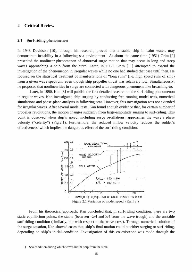
velocity (“celerity”) (Fig.2.1). Furthermore, the reduced inflow velocity reduces the rudder’s

effectiveness, which implies the dangerous effect of the surf-riding condition.

Figure 2.1 Variation of model speed, (Kan [3])

From his theoretical approach, Kan concluded that, in surf-riding condition, there are two

static equilibrium points; the stable (between –λ/4 and λ/4 from the wave trough) and the unstable

surf-riding condition (similarly, but with respect to the wave crest). Through numerical solution of

the surge equation, Kan showed cases that, ship’s final motion could be either surging or surf-riding,

depending on ship’s initial condition. Investigation of this co-existence was made through the

1) Sea condition during which waves hit the ship from the stern.

16

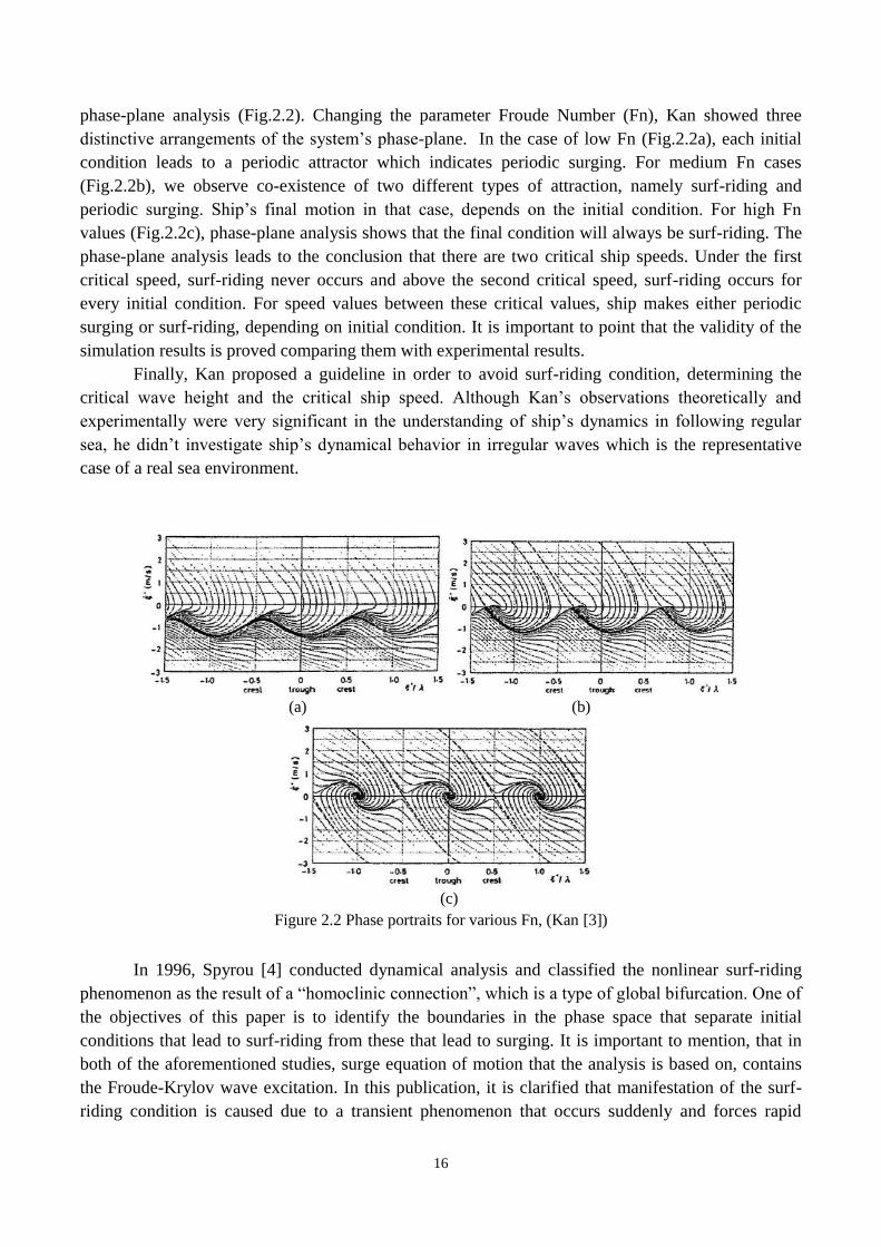
phase-plane analysis (Fig.2.2). Changing the parameter Froude Number (Fn), Kan showed three

distinctive arrangements of the system’s phase-plane. In the case of low Fn (Fig.2.2a), each initial

condition leads to a periodic attractor which indicates periodic surging. For medium Fn cases

(Fig.2.2b), we observe co-existence of two different types of attraction, namely surf-riding and

periodic surging. Ship’s final motion in that case, depends on the initial condition. For high Fn

values (Fig.2.2c), phase-plane analysis shows that the final condition will always be surf-riding. The

phase-plane analysis leads to the conclusion that there are two critical ship speeds. Under the first

critical speed, surf-riding never occurs and above the second critical speed, surf-riding occurs for

every initial condition. For speed values between these critical values, ship makes either periodic

surging or surf-riding, depending on initial condition. It is important to point that the validity of the

simulation results is proved comparing them with experimental results.

Finally, Kan proposed a guideline in order to avoid surf-riding condition, determining the

critical wave height and the critical ship speed. Although Kan’s observations theoretically and

experimentally were very significant in the understanding of ship’s dynamics in following regular

sea, he didn’t investigate ship’s dynamical behavior in irregular waves which is the representative

case of a real sea environment.

(a) (b)

(c)

Figure 2.2 Phase portraits for various Fn, (Kan [3])

In 1996, Spyrou [4] conducted dynamical analysis and classified the nonlinear surf-riding

phenomenon as the result of a “homoclinic connection”, which is a type of global bifurcation. One of

the objectives of this paper is to identify the boundaries in the phase space that separate initial

conditions that lead to surf-riding from these that lead to surging. It is important to mention, that in

both of the aforementioned studies, surge equation of motion that the analysis is based on, contains

the Froude-Krylov wave excitation. In this publication, it is clarified that manifestation of the surf-

riding condition is caused due to a transient phenomenon that occurs suddenly and forces rapid

17

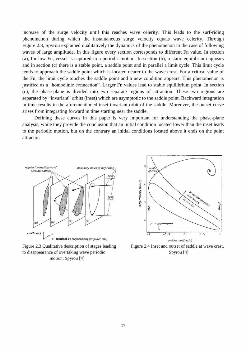
increase of the surge velocity until this reaches wave celerity. This leads to the surf-riding

phenomenon during which the instantaneous surge velocity equals wave celerity. Through

Figure 2.3, Spyrou explained qualitatively the dynamics of the phenomenon in the case of following

waves of large amplitude. In this figure every section corresponds to different Fn value. In section

(a), for low Fn, vessel is captured in a periodic motion. In section (b), a static equilibrium appears

and in section (c) there is a stable point, a saddle point and in parallel a limit cycle. This limit cycle

tends to approach the saddle point which is located nearer to the wave crest. For a critical value of

the Fn, the limit cycle touches the saddle point and a new condition appears. This phenomenon is

justified as a “homoclinic connection”. Larger Fn values lead to stable equilibrium point. In section

(c), the phase-plane is divided into two separate regions of attraction. These two regions are

separated by “invariant” orbits (inset) which are asymptotic to the saddle point. Backward integration

in time results in the aforementioned inset invariant orbit of the saddle. Moreover, the outset curve

arises from integrating forward in time starting near the saddle.

Defining these curves in this paper is very important for understanding the phase-plane

analysis, while they provide the conclusion that an initial condition located lower than the inset leads

to the periodic motion, but on the contrary an initial conditions located above it ends on the point

attractor.

Figure 2.3 Qualitative description of stages leading Figure 2.4 Inset and outset of saddle at wave crest,

to disappearance of overtaking wave periodic Spyrou [4]

motion, Spyrou [4]

18

2.2 Identification of areas with diverse dynamical behavior in phase space flows

a) Lyapunov Exponents

Alexandr Mikhailovitch Lyapunov (1857-1918) was a Russian mathematician with fundamental

contribution in stability analysis of dynamical systems. More specifically, through his doctoral thesis

“The general problem of the stability of motion” at the University of Moscow in 1892 [12], he

proposed two methods in order to define stability, the first of which was based on the linearization of

the equations of motion and the use of what was later called the Lyapunov Exponents. Lyapunov’s

research in general concentrated on investigations of stability of critical points, stability of uniformly

rotating fluid, the construction and the application of the so called “Lyapunov function”, stability of

functional differential equations, the second Lyapunov method and the method of the Lyapunov

vector function in stability theory and nonlinear analysis (Hedrih K. [13]).

Almost a century after Lyapunov’s studies on stability of motion, researchers were still trying

to explain the long-term behavior of nonlinear dynamical systems. In 1968, Oseledec develops the

theory of Lyapunov Characteristic Exponents in the frame of his study in dynamical systems and

ergodic theory [14]. In 1980, Benettin et al. [15] published research based in Oseledec’s theorem

[14], in which they proposed a method for computing the Lyapunov Charasteristic Exponents (LCE)

or maximal Lyapunov Exponent of a dynamical system. To explain their role in a few words, the

LCEs measure the rate of divergence or convergence of nearby trajectories in phase space. So, LCEs

play an important role in the study of nonlinear dynamical systems while positive LCEs imply chaos.

The gap of knowledge in the field of diagnosis of chaotic dynamical systems is going to be fulfilled

by the calculation of the Lyapunov Exponents’ spectrum.

In 1985, Wolf et al. [16] published an algorithm that computes numerically Lyapunov

Exponents of dynamical systems in time, based in Benettin et al.’s [15] method. This method was

applied in several known dynamical systems, defined by differential equations (Henon, Rossler,

Lorenz, Mackey-Glass), either autonomous or non-autonomous, and could also be applied in

experimental data. This algorithm is based upon the monitoring of the evolution of an infinitesimal

n-sphere of initial conditions, in an n-dimensional phase space (Wolf et al. [16]). In the case of one-

dimensional flow map, computation of positive LCE characterizes a system as chaotic, zero LCE as

periodic and negative LCE as stable.

Some years later, in 1996, Sandri [17], based in the computational method developed earlier

by Benettin et al. [15] and Wolf et al. [16], presented an algorithm in Mathematica in order to

compute the whole spectrum of Lyapunov Exponents for n-dimensional dynamical systems. This is

the algorithm implemented in chapter 6.1 of this thesis. An example of the LCEs computed using

Lorenz equations is presented in Fig.2.5.

Although computation of LCEs’ spectrum provides the identification of a nonlinear system’s

long-term behavior, this diagnosis does not offer visual identification of the type of attractors and the

mechanisms that lead to the system’s final condition. More specifically, the algorithm mentioned

above examines the rate of separation of trajectories corresponding to an ensemble of initial

conditions near to the reference trajectory, which means that the case of co-existence of stable

conditions is not obvious through LCEs’ spectrum. In order to overcome this and recognize

19

boundaries in the phase space that direct the flow into different dynamical behavior, more aspects of

Lyapunov exponents were introduced. More precisely, a finite version of Lyapunov exponents was

expressed through the similar methods of Finite-Time Lyapunov Exponent (FTLE) and Finite-Size

Lyapunov Exponent (FSLE), which provide comparable visualizations on the magnitude of

stretching of nearby trajectories over a finite interval of time (Haller et al. [7], Boffetta et al. [18]).

The scientific community, trying to understand transport mechanisms of time-dependent

flows, and indeed of dynamical systems, initially implemented these methods in oceanographic

research. Using FTLE or FSLE method the creation of a scalar field in phase-space is possible, in

which positive values indicate separation of nearby trajectories. In the FTLE method, a scalar field is

computed by measuring the stretching of trajectories for a determined finite period of time. On the

other hand, through the FSLE method we measure the time it takes to obtain a certain stretching

ratio. Visualization of these scalar fields provides a measure of the separation of particle trajectories

through which we recognize transport barriers of flow particles.

In the paper of Boffetta et al. [18], a comparison of FTLE and FSLE methods is made, in

parallel with an Eulerian technique applied on a two-dimensional fluid flow. Through this research it

is concluded that both methods provide better results in the identification of transport barriers from

that given by the Eulerian method. It is also proved that FTLE method seems more efficient from

FSLE in certain cases. Furthermore, in the research of Peikert et al. [19], extended comparison of the

two aforementioned methods is conducted and it is also concluded that distinguishing which method

fits the best to our problem, depends on the initial knowledge of the time or spatial scales and on our

interest on the interaction of transport mechanisms. Moreover, maximum similarity of these methods

could be achieved by choosing the appropriate parameters in the numerical computation of the scalar

field in each case.

Figure 2.5 Plot of the Lyapunov spectrum for the Lorenz model, Sandri [17]

20

b) The concept of Lagrangian Coherent Structures (LCSs)

In 2000 Haller et al. [7] introduce Lagrangian boundaries of Coherent Structures in order to explain

the transport mechanisms in time-dependent two-dimensional turbulent fluid flows. Haller presents

these boundaries as geometric structures, similar to stable and unstable manifolds of dynamical

systems, that govern fluid transport. In addition, Haller [20] proposed the “direct” computation of

largest Finite-Time Lyapunov Exponents as a tool appropriate to extract LCSs. He shows that local

maxima in the Finite-Time Lyapunov Exponent (FTLE) field are, in fact, indicators of repelling

Lagrangian Coherent Structures (LCSs) in forward time integration and of attracting LCSs in

backward time integration. He also implements the method in order to extract repelling LCSs in a 3-

Dimensional flow. In his publication Haller [21] suggests specific criteria for extracting LCSs,

applying them in several 2-Dimensional time-dependent flows, presenting in parallel specific

examples. Choosing flows that have exact solutions, he verifies the criteria he proposed. Although it

was initially believed that across these structures zero flux of material is accomplished, this

consideration changed later.

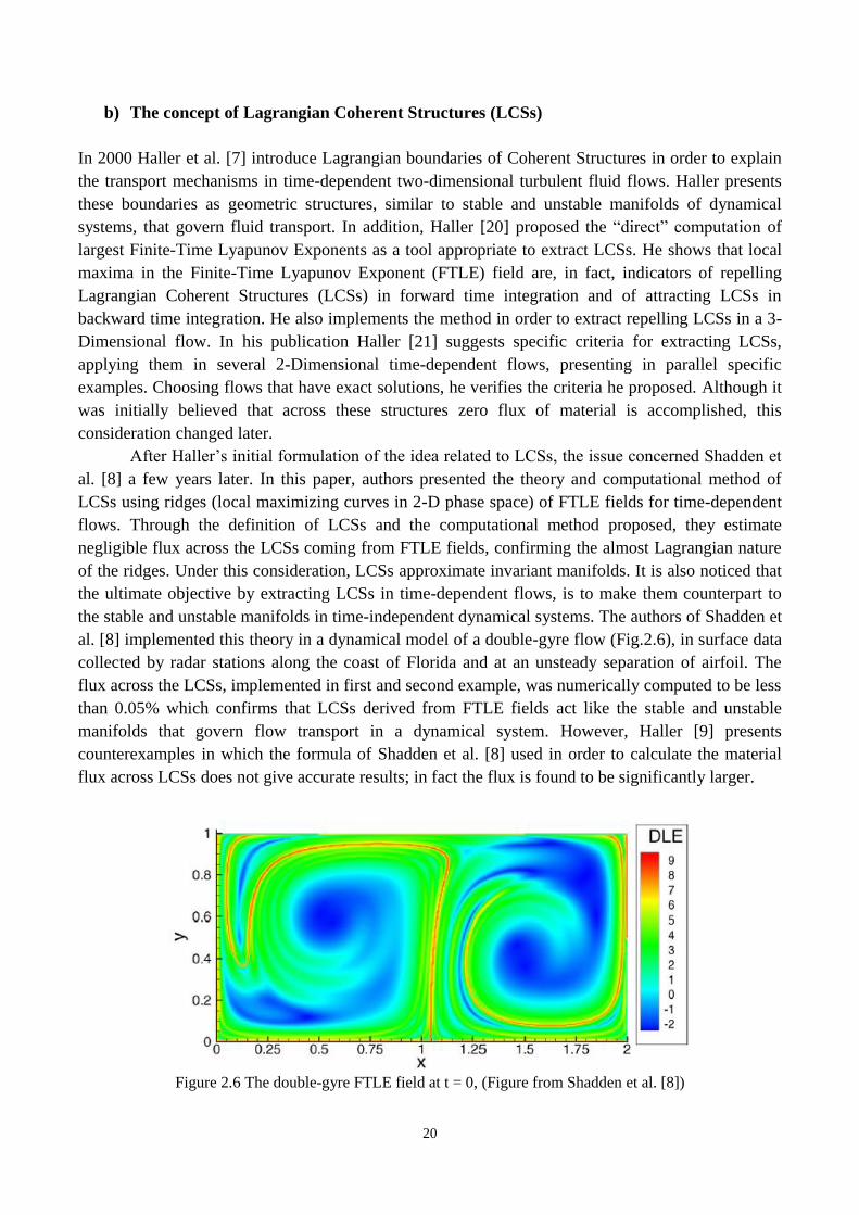
After Haller’s initial formulation of the idea related to LCSs, the issue concerned Shadden et

al. [8] a few years later. In this paper, authors presented the theory and computational method of

LCSs using ridges (local maximizing curves in 2-D phase space) of FTLE fields for time-dependent

flows. Through the definition of LCSs and the computational method proposed, they estimate

negligible flux across the LCSs coming from FTLE fields, confirming the almost Lagrangian nature

of the ridges. Under this consideration, LCSs approximate invariant manifolds. It is also noticed that

the ultimate objective by extracting LCSs in time-dependent flows, is to make them counterpart to

the stable and unstable manifolds in time-independent dynamical systems. The authors of Shadden et

al. [8] implemented this theory in a dynamical model of a double-gyre flow (Fig.2.6), in surface data

collected by radar stations along the coast of Florida and at an unsteady separation of airfoil. The

flux across the LCSs, implemented in first and second example, was numerically computed to be less

than 0.05% which confirms that LCSs derived from FTLE fields act like the stable and unstable

manifolds that govern flow transport in a dynamical system. However, Haller [9] presents

counterexamples in which the formula of Shadden et al. [8] used in order to calculate the material

flux across LCSs does not give accurate results; in fact the flux is found to be significantly larger.

Figure 2.6 The double-gyre FTLE field at t = 0, (Figure from Shadden et al. [8])

21

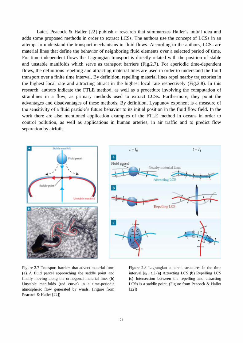
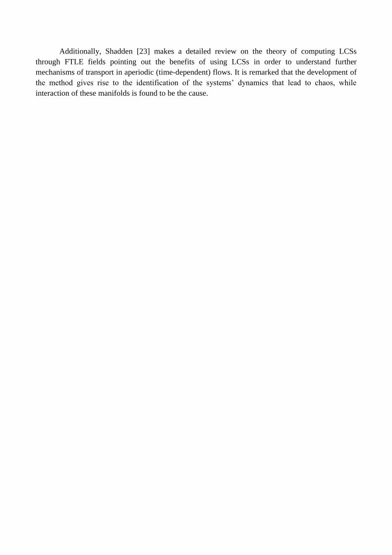
Later, Peacock & Haller [22] publish a research that summarizes Haller’s initial idea and

adds some proposed methods in order to extract LCSs. The authors use the concept of LCSs in an

attempt to understand the transport mechanisms in fluid flows. According to the authors, LCSs are

material lines that define the behavior of neighboring fluid elements over a selected period of time.

For time-independent flows the Lagrangian transport is directly related with the position of stable

and unstable manifolds which serve as transport barriers (Fig.2.7). For aperiodic time-dependent

flows, the definitions repelling and attracting material lines are used in order to understand the fluid

transport over a finite time interval. By definition, repelling material lines repel nearby trajectories in

the highest local rate and attracting attract in the highest local rate respectively (Fig.2.8). In this

research, authors indicate the FTLE method, as well as a procedure involving the computation of

strainlines in a flow, as primary methods used to extract LCSs. Furthermore, they point the

advantages and disadvantages of these methods. By definition, Lyapunov exponent is a measure of

the sensitivity of a fluid particle’s future behavior to its initial position in the fluid flow field. In the

work there are also mentioned application examples of the FTLE method in oceans in order to

control pollution, as well as applications in human arteries, in air traffic and to predict flow

separation by airfoils.

Figure 2.7 Transport barriers that advect material form

(a) A fluid parcel approaching the saddle point and

finally moving along the orthogonal material line. (b)

Unstable manifolds (red curve) in a time-periodic

atmospheric flow generated by winds, (Figure from

Peacock & Haller [22])

Figure 2.8 Lagrangian coherent structures in the time

interval [t0 , t1].(a) Attracting LCS (b) Repelling LCS

(c) Intersection between the repelling and attracting

LCSs is a saddle point, (Figure from Peacock & Haller

[22])

Additionally, Shadden [23] makes a detailed review on the theory of computing LCSs

through FTLE fields pointing out the benefits of using LCSs in order to understand further

mechanisms of transport in aperiodic (time-dependent) flows. It is remarked that the development of

the method gives rise to the identification of the systems’ dynamics that lead to chaos, while

interaction of these manifolds is found to be the cause.

23

3 Objectives

The main objectives of this thesis are:

The implementation of new numerical tools, already used in the understanding of

mechanisms that lead fluid transport in fluid flows, in order to gain insight into the

mechanisms leading to the surf-riding phenomenon that usually causes ship’s instability

through broaching-to in following seas.

To apply numerical methods in order to diagnose chaotic ship’s response in following seas.

To apply the aforementioned methods firstly in regular wave excitation in order to test their

applicability, secondary in bi-chromatic wave excitation and finally in multi-chromatic wave

environment.

24

25

4 Equation of surge motion

4.1 General equation form

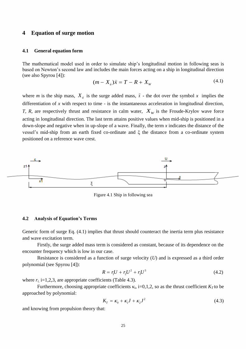
The mathematical model used in order to simulate ship’s longitudinal motion in following seas is

based on Newton’s second law and includes the main forces acting on a ship in longitudinal direction

(see also Spyrou [4]): (4.1)

where m is the ship mass, uX is the surge added mass, x - the dot over the symbol x implies the

differentiation of x with respect to time - is the instantaneous acceleration in longitudinal direction,

T, R, are respectively thrust and resistance in calm water, WX is the Froude-Krylov wave force

acting in longitudinal direction. The last term attains positive values when mid-ship is positioned in a

down-slope and negative when in up-slope of a wave. Finally, the term x indicates the distance of the

vessel’s mid-ship from an earth fixed co-ordinate and ξ the distance from a co-ordinate system

positioned on a reference wave crest.

Figure 4.1 Ship in following sea

4.2 Analysis of Equation’s Terms

Generic form of surge Eq. (4.1) implies that thrust should counteract the inertia term plus resistance

and wave excitation term.

Firstly, the surge added mass term is considered as constant, because of its dependence on the

encounter frequency which is low in our case.

Resistance is considered as a function of surge velocity (U) and is expressed as a third order

polynomial (see Spyrou [4]):

2 3

1 2 3R rU rU rU (4.2)

where ri, i=1,2,3, are appropriate coefficients (Table 4.3).

Furthermore, choosing appropriate coefficients κi, i=0,1,2, so as the thrust coefficient KT to be

approached by polynomial:

2

0 1 2TK J J (4.3)

and knowing from propulsion theory that:

( )u Wm X x T R X

26

(1 )pU

JnD

(4.4)

we express thrust as a polynomial of second order depending on surge velocity (U) and propeller’s

rate (n):

2 2

0 1 2T n nU U (4.5)

where τi, i=0,1,2, are coefficients conveyed by following forms:

4

0 0

3

1 1

2 2

2 2

(1 )

(1 )(1 )

(1 )(1 )

p

p p

p p

t D

t D

t D

(4.6)

where tp is the thrust deduction coefficient and ωp is the wake fraction coefficient, considering still

water for both cases. Moreover, D and n are respectively the propeller diameter and rate.

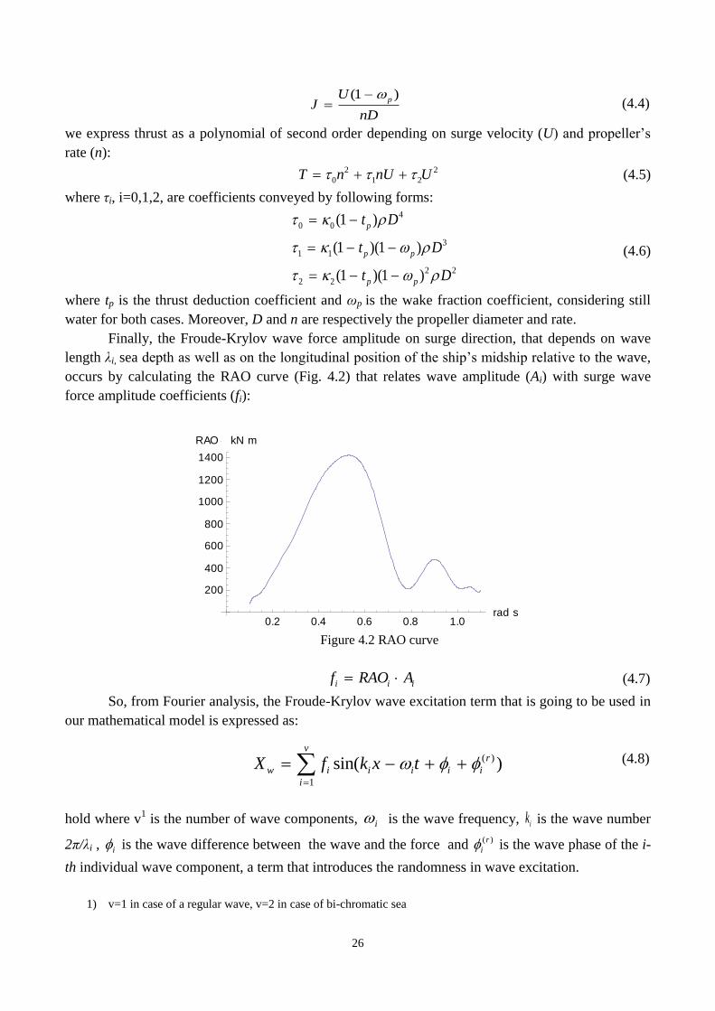
Finally, the Froude-Krylov wave force amplitude on surge direction, that depends on wave

length λi, sea depth as well as on the longitudinal position of the ship’s midship relative to the wave,

occurs by calculating the RAO curve (Fig. 4.2) that relates wave amplitude (Ai) with surge wave

force amplitude coefficients (fi):

Figure 4.2 RAO curve

i i if RAO A (4.7)

So, from Fourier analysis, the Froude-Krylov wave excitation term that is going to be used in

our mathematical model is expressed as:

(4.8)

hold where v1 is the number of wave components, i is the wave frequency, ik is the wave number

2π/λi , i is the wave difference between the wave and the force and ( )r

i is the wave phase of the i-

th individual wave component, a term that introduces the randomness in wave excitation.

1) v=1 in case of a regular wave, v=2 in case of bi-chromatic sea

0.2 0.4 0.6 0.8 1.0rad s

200

400

600

800

1000

1200

1400

RAO kN m

( )

1

sin( )v

r

w i i i i i

i

X f k x t

27

4.3 Final Ship’s Surge Motion Equation

a) Non-autonomous form of nonlinear equation of surging motion

Substituting expressions (4.2), (4.3), (4.8) in (4.1), assuming fixed on earth co-ordinate system, we

obtain:

3 2 2

3 2 2 1 1 0

1

      sinr

u i i i i im X x r r x r x f k nx x t

(4.9)

b) Autonomous form of nonlinear equation of surging motion for regular wave excitation

In the above model we assumed so far a co-ordinate system fixed on earth. In case we prefer to

obtain an autonomous version of the equation, consideration that is applicable only for regular wave

excitation, we have to define a new moving co-ordinate system, positioned on the crest of a reference

wave and moving with the wave phase velocity c. In parallel, we replace variable x with

x c t , where ξ represents the surge distance from the new co-ordinate system (see Fig.4.1).

Now, the new expressions are:

From (4.1): ( )u Wm X T R X (4.10)

From (4.8): sin( )wX f k (4.11)

Substituting expressions (4.2), (4.3), (4.1) in (4.9), and considering the transformation

U c , where c = ω/k is the wave celerity, the following equation occurs:

2 2 3

3 2 2 1 1 3 2 2 3

2 2 3

0 1 1 2 2 3

( ) [3 2( ) ] [3 ( )]

sin( ) ( )

um X r c r c r n r c r r

f k n rc cn r c r c

(4.12)

The above autonomous form of the surge equation is problematic in polychromatic wave

excitation. The transformation x c t used above to annihilate time is not applicable due to

the existence of the constant term of wave celerity c, which differs for every wave. So, Eq.(4.12) is

implemented only in the regular case (v=1).

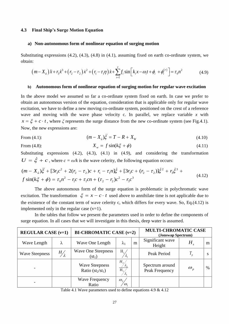
In the tables that follow we present the parameters used in order to define the components of

surge equation. In all cases that we will investigate in this thesis, deep water is assumed.

REGULAR CASE (ν=1) BI-CHROMATIC CASE (ν=2) MULTI-CHROMATIC CASE

(Jonswap Spectrum)

Wave Length λ Wave One Length λ1 m Significant wave

Height sH m

Wave Steepness H

Wave One Steepness

(st1) 1

1 Peak Period pT s

- Wave Steepness

Ratio (st2/st1)

2

2

1

1

H

Spectrum around

Peak Frequency p %

- Wave Frequency

Ratio 2

1

Table 4.1 Wave parameters used to define equations 4.9 & 4.12

28

Parameters’ names Symbol Units

Ship’s Nominal Speed unom m/s

Ship’s Initial Position x0 m

Ship’s Initial Speed u0 m/s

Initial Time t0 s

Table 4.2 Ship parameters used to define equation 4.9 & 4.12

Concluding, a generic form of ship’s surge equation (Eq.(4.9), Eq.(4.12)) is used in our

mathematical model in order to simulate ship’s motion in following seas, either regular, bi-

chromatic or irregular.

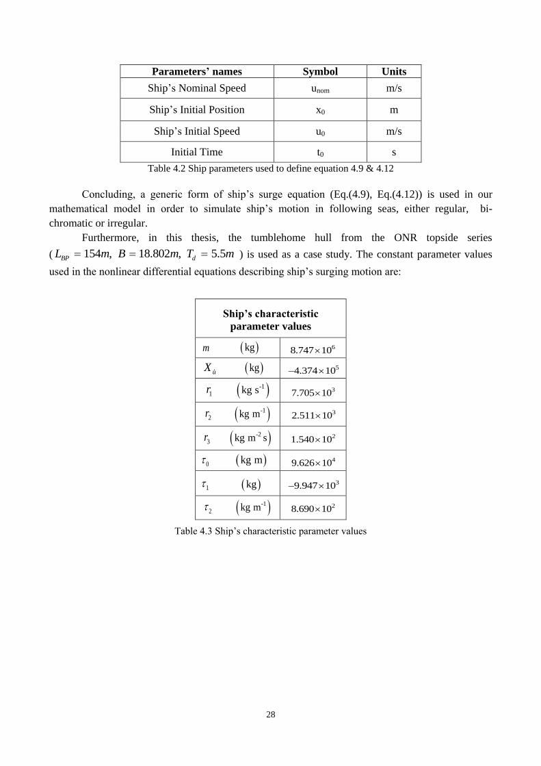
Furthermore, in this thesis, the tumblehome hull from the ONR topside series

( 154 , 18.802 , 5.5BP dL m B m T m ) is used as a case study. The constant parameter values

used in the nonlinear differential equations describing ship’s surging motion are:

Table 4.3 Ship’s characteristic parameter values

Ship’s characteristic

parameter values

 m

  kg 68.747 10

  uX

  kg 5  4.374 10

1r -1  kg s 3 7.705 10

2r -1kg m 3 2.511 10

3r -2  kg m s 21  .540 10

0   kg m 4 9.626 10

1   kg 3  9.947 10

2 -1  kg m 2 8.690 10

29

5 Dynamical Systems

5.1 Stability of dynamical systems

It is commonly accepted that solutions of differential equations have the capability to simulate the

behavior of a physical phenomenon. Furthermore, existing mathematical tools provide us an

approach on the system’s long-term asymptotic motion. The main objective of this chapter is to

concisely provide notions of the theory of dynamical systems that are going to be used later in this

thesis.

The solution of an n-dimensional dynamical system described by n time-dependent

differential equations:

1 1 1( ) ( ( ),..., ( ), )nx t f x t x t t

(5.1)

1( ) ( ( ),..., ( ), )n n nx t f x t x t t

represents a curve embedded in a n-dimensional space with coordinates ( 1( )x t , 2 ( )x t ,… ( )nx t ). This

space is commonly referred as “phase-space” (“phase-plane” in case of n=2). The system’s solutions

constitute a trajectory (function of time) moving on the 1 2( , ,..., )nx x x phase space starting from the

initial condition 1 0 2 0 0( ( ), ( ),..., ( ))nx t x t x t at time 0t .

Henceforth, let’s consider a two-dimensional autonomous dynamical system (n=2) in order to

simplify our analysis:

1 1 1 2( ) ( ( ), ( ))x t f x t x t

2 2 1 2( ) ( ( ), ( ))x t f x t x t or the vector form:

( ) ( ( ))x t F x t (5.2)

In this case, solutions in the two-dimensional phase-space are described in variables of

( 1 2( ), ( )x t x t ).In order to identify the long-term behavior of a dynamical system in the phase space,

we use differential equations to construct a vector field, through which we assign a velocity vector

1 2( ) ( ( ), ( ))x t x t x t at each 1 2( ) ( ( ), ( ))x t x t x t . The velocity vector field is provided if we plot the

corresponding velocity vector in the tangent space of each trajectory, which is represented by:

1 2( ( )) ( ( ), ( ))F x t x t x t (5.3)

This vector field determines the way the two-dimensional trajectory 1 2( ) ( ( ), ( ))x t x t x t is

going to be developed while time passes and consequently indicates the long-term qualitative

behavior of a dynamical system. Depiction of trajectories in the phase plane, the arrangement of

30

which is associated with the vector field represents the “phase portrait” of a dynamical system.

Through phase portraits we obtain information on the system’s equilibrium solutions, defined by:

*( ) 0F x (5.4)

A system that ends up on a point of equilibrium*x , is stabilized in this condition for all t.

Equilibrium points (or stationary states) are categorized in stable and unstable equilibrium points. If

infinitesimal disturbances away of the stationary state are damped out in time, then this state is

characterized as stable. In opposite case, that disturbances tend to grow, we have unstable stationary

state. Generally, we use the term of a limit set in order to express the geometric structure of a steady

state that a system is going to obtain asymptotically in a phase portrait as t . We recognize three

main categories of limit sets:

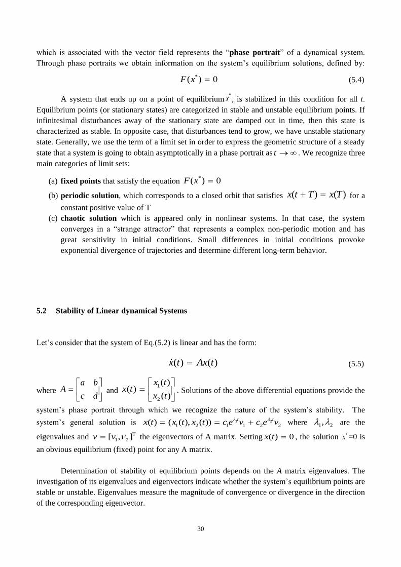
(a) fixed points that satisfy the equation *( ) 0F x

(b) periodic solution, which corresponds to a closed orbit that satisfies ( ) ( )x t T x T for a

constant positive value of T

(c) chaotic solution which is appeared only in nonlinear systems. In that case, the system

converges in a “strange attractor” that represents a complex non-periodic motion and has

great sensitivity in initial conditions. Small differences in initial conditions provoke

exponential divergence of trajectories and determine different long-term behavior.

5.2 Stability of Linear dynamical Systems

Let’s consider that the system of Eq.(5.2) is linear and has the form:

( ) ( )x t Ax t (5.5)

where a b

Ac d

and 1

2

( )( )

( )

x tx t

x t

. Solutions of the above differential equations provide the

system’s phase portrait through which we recognize the nature of the system’s stability. The

system’s general solution is 1 2

1 2 1 1 2 2( ) ( ( ), ( ))t t

x t x t x t c e v c e v

where 1 2, are the

eigenvalues and 1 2[ , ]v v the eigenvectors of A matrix. Setting ( ) 0x t , the solution *x =0 is

an obvious equilibrium (fixed) point for any A matrix.

Determination of stability of equilibrium points depends on the A matrix eigenvalues. The

investigation of its eigenvalues and eigenvectors indicate whether the system’s equilibrium points are

stable or unstable. Eigenvalues measure the magnitude of convergence or divergence in the direction

of the corresponding eigenvector.

31

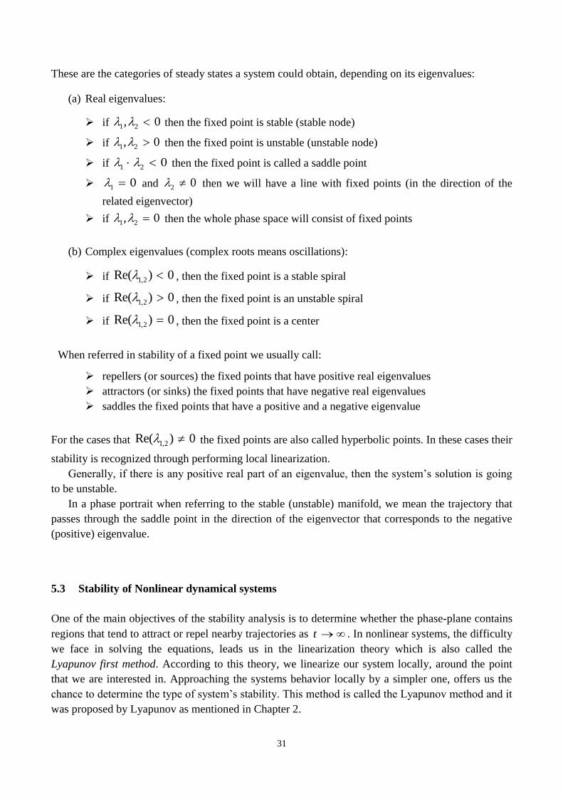
These are the categories of steady states a system could obtain, depending on its eigenvalues:

(a) Real eigenvalues:

if 1 2, 0 then the fixed point is stable (stable node)

if 1 2, 0 then the fixed point is unstable (unstable node)

if 1 2 0 then the fixed point is called a saddle point

1 0 and 2 0 then we will have a line with fixed points (in the direction of the

related eigenvector)

if 1 2, 0 then the whole phase space will consist of fixed points

(b) Complex eigenvalues (complex roots means oscillations):

if 1,2Re( ) 0 , then the fixed point is a stable spiral

if 1,2Re( ) 0 , then the fixed point is an unstable spiral

if 1,2Re( ) 0 , then the fixed point is a center

When referred in stability of a fixed point we usually call:

repellers (or sources) the fixed points that have positive real eigenvalues

attractors (or sinks) the fixed points that have negative real eigenvalues

saddles the fixed points that have a positive and a negative eigenvalue

For the cases that 1,2Re( ) 0 the fixed points are also called hyperbolic points. In these cases their

stability is recognized through performing local linearization.

Generally, if there is any positive real part of an eigenvalue, then the system’s solution is going

to be unstable.

In a phase portrait when referring to the stable (unstable) manifold, we mean the trajectory that

passes through the saddle point in the direction of the eigenvector that corresponds to the negative

(positive) eigenvalue.

5.3 Stability of Nonlinear dynamical systems

One of the main objectives of the stability analysis is to determine whether the phase-plane contains

regions that tend to attract or repel nearby trajectories as t . In nonlinear systems, the difficulty

we face in solving the equations, leads us in the linearization theory which is also called the

Lyapunov first method. According to this theory, we linearize our system locally, around the point

that we are interested in. Approaching the systems behavior locally by a simpler one, offers us the

chance to determine the type of system’s stability. This method is called the Lyapunov method and it

was proposed by Lyapunov as mentioned in Chapter 2.

32

Let’s consider the nonlinear system of Eq.(5.1), * * *

1( ,..., )nx x x to be a fixed point and

1( ,..., )ny y y to be the distance of a nearby point (perturbation) in the phase-plane. After these

considerations each of the system’s equations is approached by:

* * * *

1 1 1

1

( ) ( ,..., ) ( ) ...Taylor

i ii i n n i n

n

f ff x y f x y x y f x y y

x x

,i=1,..,n (5.6)

where the term *( )if x equals to zero. So, the general form of the linearized system is:

*

1 1

*1 11

*

1

( )

( )

n

n n nn

n x x

f f

x x yf x y

f f yf x y

x x

or *( )x F x y Ay (5.7)

where A is the jacobian matrix of f evaluated at *x x .

Then, determining the eigenvalues of the jacobian matrix A, in case of hyperbolic fixed points

we are able to define their stability (stable, unstable, saddle). Furthermore, Lyapunov, in his attempt

to analyze stability of nonlinear dynamical systems, also developed the second Lyapunov method

which is based on the construction of the Lyapunov Function, through which we can make a

conjecture about the system’s stability. However, the absence of a general formula that defines these

functions makes it difficult to use them in practice.

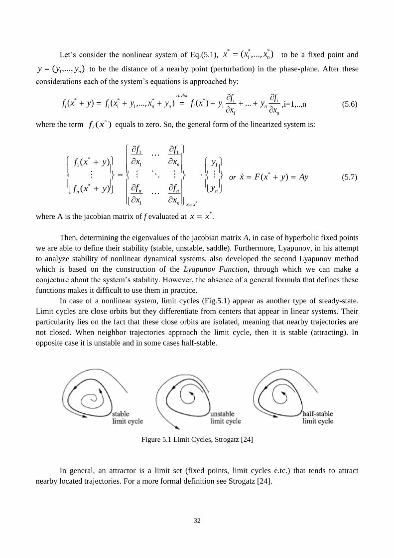
In case of a nonlinear system, limit cycles (Fig.5.1) appear as another type of steady-state.

Limit cycles are close orbits but they differentiate from centers that appear in linear systems. Their

particularity lies on the fact that these close orbits are isolated, meaning that nearby trajectories are

not closed. When neighbor trajectories approach the limit cycle, then it is stable (attracting). In

opposite case it is unstable and in some cases half-stable.

Figure 5.1 Limit Cycles, Strogatz [24]

In general, an attractor is a limit set (fixed points, limit cycles e.tc.) that tends to attract

nearby located trajectories. For a more formal definition see Strogatz [24].

33

5.4 Bifurcations of dynamical systems

From previous paragraphs, through the system’s phase portrait, we recognize whether limit sets are

stable or unstable. However, the nature of the system’s limit set depends on the system’s parameters.

Variation on these parameters incurs changing in the trajectories’ structure and as a result in the

topology of the phase portrait. This implies the creation and the disappearance of limit sets or even

change in their stability. This change in the dynamical behavior is called bifurcation phenomenon.

The parameter values at which such a phenomenon appears are called bifurcation points.

Some of the most common types of bifurcation are: saddle-node bifurcation, transcritical

bifurcation, pitchfork bifurcation (supercritical or subcritical), hopf bifurcation, saddle bifurcation of

cycles, infinite-period bifurcation and homoclinic bifurcation (Strogatz [24]). Homoclinic bifurcation

is the phenomenon we are going to focus in detail while it is straightly connected with surf-riding

phenomenon.

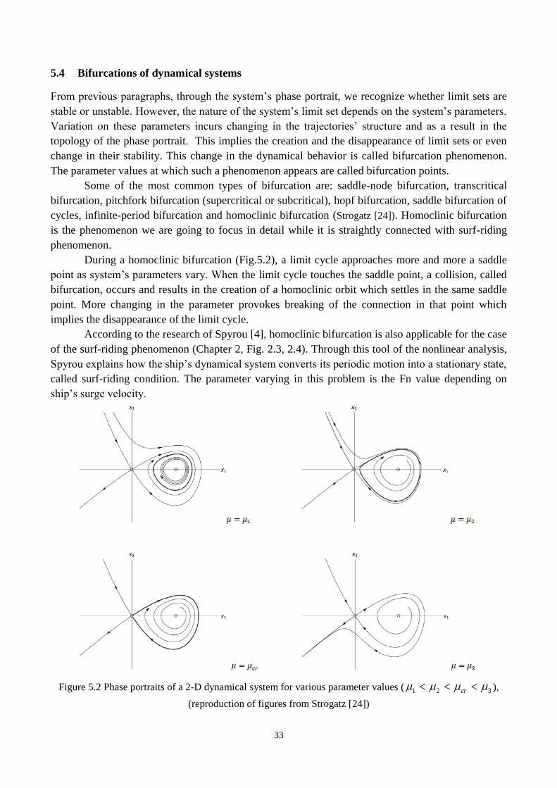
During a homoclinic bifurcation (Fig.5.2), a limit cycle approaches more and more a saddle

point as system’s parameters vary. When the limit cycle touches the saddle point, a collision, called

bifurcation, occurs and results in the creation of a homoclinic orbit which settles in the same saddle

point. More changing in the parameter provokes breaking of the connection in that point which

implies the disappearance of the limit cycle.

According to the research of Spyrou [4], homoclinic bifurcation is also applicable for the case

of the surf-riding phenomenon (Chapter 2, Fig. 2.3, 2.4). Through this tool of the nonlinear analysis,

Spyrou explains how the ship’s dynamical system converts its periodic motion into a stationary state,

called surf-riding condition. The parameter varying in this problem is the Fn value depending on

ship’s surge velocity.

Figure 5.2 Phase portraits of a 2-D dynamical system for various parameter values ( 1 2 3cr ),

(reproduction of figures from Strogatz [24])

34

35

6 Numerical tools for investigating dynamical systems

6.1 Lyapunov Characteristic Exponents

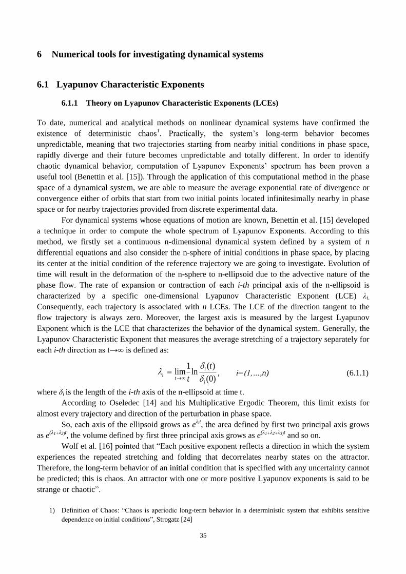
6.1.1 Theory on Lyapunov Characteristic Exponents (LCEs)

To date, numerical and analytical methods on nonlinear dynamical systems have confirmed the

existence of deterministic chaos1. Practically, the system’s long-term behavior becomes

unpredictable, meaning that two trajectories starting from nearby initial conditions in phase space,

rapidly diverge and their future becomes unpredictable and totally different. In order to identify

chaotic dynamical behavior, computation of Lyapunov Exponents’ spectrum has been proven a

useful tool (Benettin et al. [15]). Through the application of this computational method in the phase

space of a dynamical system, we are able to measure the average exponential rate of divergence or

convergence either of orbits that start from two initial points located infinitesimally nearby in phase

space or for nearby trajectories provided from discrete experimental data.

For dynamical systems whose equations of motion are known, Benettin et al. [15] developed

a technique in order to compute the whole spectrum of Lyapunov Exponents. According to this

method, we firstly set a continuous n-dimensional dynamical system defined by a system of n

differential equations and also consider the n-sphere of initial conditions in phase space, by placing

its center at the initial condition of the reference trajectory we are going to investigate. Evolution of

time will result in the deformation of the n-sphere to n-ellipsoid due to the advective nature of the

phase flow. The rate of expansion or contraction of each i-th principal axis of the n-ellipsoid is

characterized by a specific one-dimensional Lyapunov Characteristic Exponent (LCE) λi.

Consequently, each trajectory is associated with n LCEs. The LCE of the direction tangent to the

flow trajectory is always zero. Moreover, the largest axis is measured by the largest Lyapunov

Exponent which is the LCE that characterizes the behavior of the dynamical system. Generally, the

Lyapunov Characteristic Exponent that measures the average stretching of a trajectory separately for

each i-th direction as t→∞ is defined as:

( )1

lim ln(0)

ii

ti

t

t

, i=(1,…,n) (6.1.1)

where δi is the length of the i-th axis of the n-ellipsoid at time t.

According to Oseledec [14] and his Multiplicative Ergodic Theorem, this limit exists for

almost every trajectory and direction of the perturbation in phase space.

So, each axis of the ellipsoid grows as eλit, the area defined by first two principal axis grows

as e(λ1+λ2)t, the volume defined by first three principal axis grows as e

(λ1+λ2+λ3)t and so on.

Wolf et al. [16] pointed that “Each positive exponent reflects a direction in which the system

experiences the repeated stretching and folding that decorrelates nearby states on the attractor.

Therefore, the long-term behavior of an initial condition that is specified with any uncertainty cannot

be predicted; this is chaos. An attractor with one or more positive Lyapunov exponents is said to be

strange or chaotic”.

1) Definition of Chaos: “Chaos is aperiodic long-term behavior in a deterministic system that exhibits sensitive

dependence on initial conditions”, Strogatz [24]

36

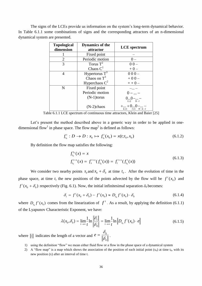
The signs of the LCEs provide us information on the system’s long-term dynamical behavior.

In Table 6.1.1 some combinations of signs and the corresponding attractors of an n-dimensional

dynamical system are presented.

Topological

dimension

Dynamics of the

attractor LCE spectrum

1 Fixed point –

2 Periodic motion 0 –

3 Torus T2

Chaos C1

0 0 –

+ 0 –

4 Hypertorus T3

Chaos on T3

Hyperchaos C2

0 0 0 –

+ 0 0 –

+ + 0 –

N Fixed point

Periodic motion

(N-1)torus

(N-2)chaos

...

0 ...

20...0 ...

l N l

1 1... 0...0 ...k l N k l

Table 6.1.1 LCE spectrum of continuous time attractors, Klein and Baier [25]

Let’s present the method described above in a generic way in order to be applied in one-

dimensional flow1 in phase space. The flow map

2 is defined as follows:

0 00 0 0 0: : ( ) ( ; , )t t

t tf D D x f x x t t x (6.1.2)

By definition the flow map satisfies the following:

0

0

0 0 0

( )

( ) ( ( )) ( ( ))

t

t

t s t s s t s t

t s t t t

f x x

f x f f x f f x

(6.1.3)

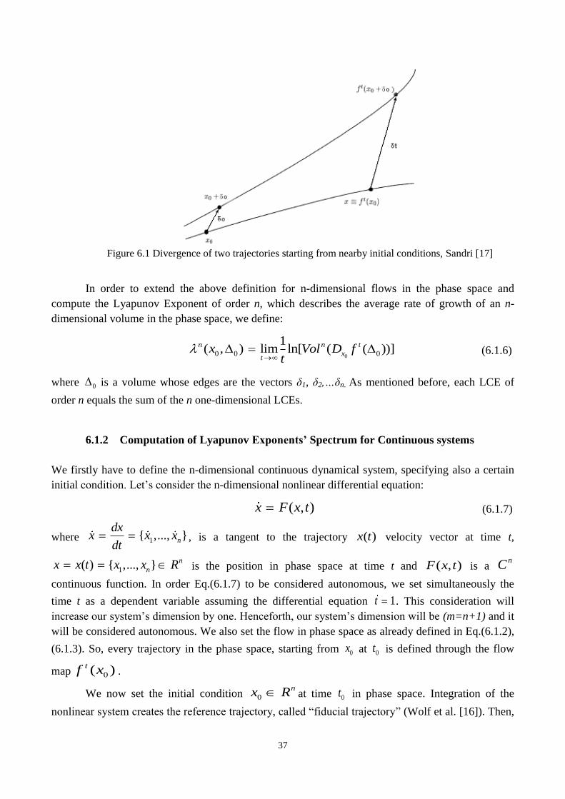
We consider two nearby points 0x and 0 0x at time 0t . After the evolution of time in the

phase space, at time t, the new positions of the points advected by the flow will be 0( )tf x and

0 0( )tf x respectively (Fig. 6.1). Now, the initial infinitesimal separation δ0 becomes:

00 0 0 0 0( ) ( ) ( )t t t

t xf x f x D f x (6.1.4)

where 0 0( )t

xD f x comes from the linearization of tf . As a result, by applying the definition (6.1.1)

of the Lyapunov Characteristic Exponent, we have:

00 0 0

0

1 1( , ) lim ln lim ln ( )

t t

xt t

x D f x et t

(6.1.5)

where indicates the length of a vector and 0

0

e

.

1) using the definition “flow” we mean either fluid flow or a flow in the phase space of a dynamical system

2) A “flow map” is a map which shows the association of the position of each initial point (x0) at time t0, with its

new position (x) after an interval of time t.

37

Figure 6.1 Divergence of two trajectories starting from nearby initial conditions, Sandri [17]

In order to extend the above definition for n-dimensional flows in the phase space and

compute the Lyapunov Exponent of order n, which describes the average rate of growth of an n-

dimensional volume in the phase space, we define:

00 0 0

1( , ) lim ln[ ( ( ))]n n t

xt

x Vol D ft

(6.1.6)

where 0 is a volume whose edges are the vectors δ1, δ2,…δn. As mentioned before, each LCE of

order n equals the sum of the n one-dimensional LCEs.

6.1.2 Computation of Lyapunov Exponents’ Spectrum for Continuous systems

We firstly have to define the n-dimensional continuous dynamical system, specifying also a certain

initial condition. Let’s consider the n-dimensional nonlinear differential equation:

( , )x F x t (6.1.7)

where 1{ ,..., }n

dxx x x

dt , is a tangent to the trajectory ( )x t velocity vector at time t,

1( ) { ,..., } n

nx x t x x R is the position in phase space at time t and ( , )F x t is a nC

continuous function. In order Eq.(6.1.7) to be considered autonomous, we set simultaneously the

time t as a dependent variable assuming the differential equation 1t . This consideration will

increase our system’s dimension by one. Henceforth, our system’s dimension will be (m=n+1) and it

will be considered autonomous. We also set the flow in phase space as already defined in Eq.(6.1.2),

(6.1.3). So, every trajectory in the phase space, starting from 0x at 0t is defined through the flow

map 0( )tf x .

We now set the initial condition 0

nx R at time 0t in phase space. Integration of the

nonlinear system creates the reference trajectory, called “fiducial trajectory” (Wolf et al. [16]). Then,

38

we consider a deviation 0( )t x from the initial condition which is expressed through a frame of

orthonormal vectors that define a sphere infinitesimally near the “fiducial trajectory”. This

perturbation evolves in time by solving the linearized equation of motion, expressed in the following

mxm matrix form:

0 0 0( ) ( ( )) ( )t

t x tx D F f x x (6.1.8)

, considering initial condition0 0( )t mx I .

In the above equation, 0( )t x is the derivative with respect to 0x of tf at 0x ( 0( )t x

=0 0( )t

xD f x ) and constitutes a set of vectors 1 2{ , ,..., }t t t

m . However, we have to notice that solving

Eq.(6.1.8) is problematic due to the fact that parts of it depend on the solution of Eq. (6.1.7).

Therefore, integration of the combined system is prerequisite in order to compute the trajectory:

0

0 0 0

( ) ( ( )),

( ) ( ( )) ( )

t

tt x t

x t F f x

x D F f x x

0 0

0

( )

( )

x t x

t

(6.1.9)

Linearized equations of motion act on the initial frame of orthonormal vectors by integrating

them for m different initial conditions so as to give a new set of vectors {δ1, δ2,…,δm}. The “fiducial

trajectory”, which is the trajectory that passes through the center of the m-sphere, is defined by

integrating the nonlinear equation of motion (Eq.6.1.9). However, an obstacle appears while

applying the combined system’s integration. Although each vector has a different magnitude, they

have the tension to end up on the direction of the fastest growth. According to Benettin et al. [15], to

avoid this, the Gram-Schmidt method of reorthonormalization is repeatedly applied on the vector

frame obtained by integration (see also Wolf et al. [16]). Through this procedure, vector δ1 will

finally coincide with the direction of largest growth.

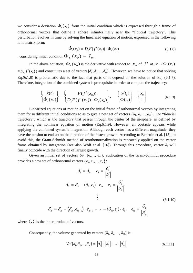
Given an initial set of vectors {δ1, δ2,…, δm}, application of the Gram-Schmidt procedure

provides a new set of orthonormal vectors 1 2, ,..., me e e :

'' 1

1 1 1 '

1

'' 22 2 2 1 1 2 '

2

,

, ,

e

e e e

(6.1.10)

''

1 1 1 1 ', , , m

m m m m m m m

m

e e e e e

where , is the inner product of vectors.

Consequently, the volume generated by vectors {δ1, δ2,…, δm} is:

' ' '

1 2 1 2{ , ,..., }m mVol (6.1.11)

39

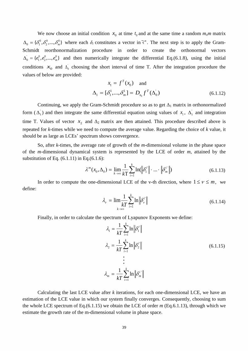
We now choose an initial condition 0x at time 0t and at the same time a random mxm matrix

0 0 0

0 1 2{ , ,..., }m where each δi constitutes a vector in m . The next step is to apply the Gram-

Schmidt reorthonormalization procedure in order to create the orthonormal vectors ' 0 0 0

0 1 2{ , ,..., }me e e and then numerically integrate the differential Eq.(6.1.8), using the initial

conditions 0x and '

0 choosing the short interval of time T. After the integration procedure the

values of below are provided:

1 0( )Tx f x and

0

1 1 '

1 1 0[ ,..., ] ( )T

m xD f (6.1.12)

Continuing, we apply the Gram-Schmidt procedure so as to get Δ1 matrix in orthonormalized

form ('

1 ) and then integrate the same differential equation using values of 1x , '

1 and integration

time T. Values of vector 2x and Δ2 matrix are then attained. This procedure described above is

repeated for k-times while we need to compute the average value. Regarding the choice of k value, it

should be as large as LCEs’ spectrum shows convergence.

So, after k-times, the average rate of growth of the m-dimensional volume in the phase space

of the m-dimensional dynamical system is represented by the LCE of order m, attained by the

substitution of Eq. (6.1.11) in Eq.(6.1.6):

' '

0 0 1

1

1( , ) lim ln( ... )

km i i

mk

i

xk

(6.1.13)

In order to compute the one-dimensional LCE of the v-th direction, where 1 m , we

define:

'

1

1lim ln

ki

ik

kT

(6.1.14)

Finally, in order to calculate the spectrum of Lyapunov Exponents we define:

'

1 1

1

1ln

ki

ikT

'

2 2

1

1ln

ki

ikT

(6.1.15)

'

1

1ln

ki

m m

ikT

Calculating the last LCE value after k iterations, for each one-dimensional LCE, we have an

estimation of the LCE value in which our system finally converges. Consequently, choosing to sum

the whole LCE spectrum of Eq.(6.1.15) we obtain the LCE of order m (Eq.6.1.13), through which we

estimate the growth rate of the m-dimensional volume in phase space.

40

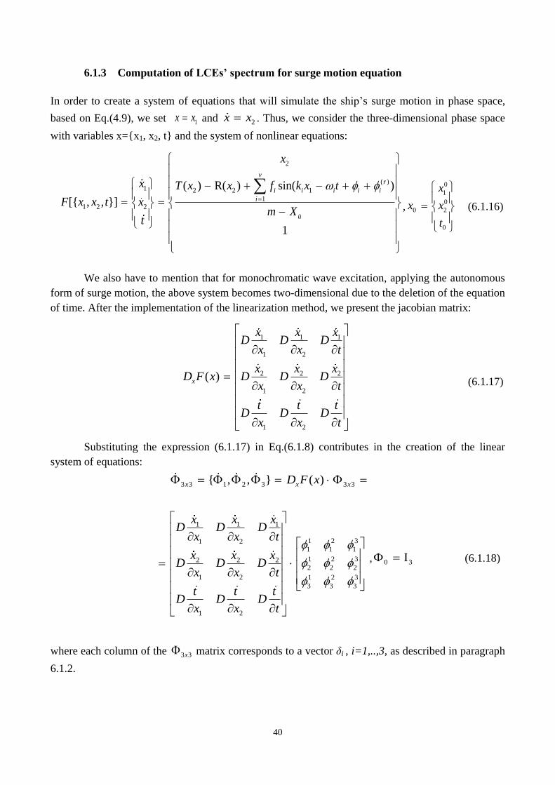
6.1.3 Computation of LCEs’ spectrum for surge motion equation

In order to create a system of equations that will simulate the ship’s surge motion in phase space,

based on Eq.(4.9), we set 1x x and 2x x . Thus, we consider the three-dimensional phase space

with variables x={x1, x2, t} and the system of nonlinear equations:

2

( )1 2 2 1

11 2 2

( ) R( ) sin( )

[{ , , }]

1

vr

i i i i i

i

u

x

x T x x f k x t

F x x t xm X

t

,

0

1

0

0 2

0

x

x x

t

(6.1.16)

We also have to mention that for monochromatic wave excitation, applying the autonomous

form of surge motion, the above system becomes two-dimensional due to the deletion of the equation

of time. After the implementation of the linearization method, we present the jacobian matrix:

1 1 1

1 2

2 2 2

1 2

1 2

( )x

x x xD D D

x x t

x x xD F x D D D

x x t

t t tD D D

x x t

(6.1.17)

Substituting the expression (6.1.17) in Eq.(6.1.8) contributes in the creation of the linear

system of equations:

3 3 1 2 3 3 3

1 1 1

1 2 31 2

1 1 1

1 2 32 2 22 2 2

1 2 1 2 3

3 3 3

1 2

{ , , } ( )x x xD F x

x x xD D D

x x t

x x xD D D

x x t

t t tD D D

x x t

, 0 3 (6.1.18)

where each column of the 3 3x matrix corresponds to a vector δi , i=1,..,3, as described in paragraph

6.1.2.

41

Having defined the system of equations that describe the flow in the phase space and the n-

sphere of initial conditions around a “fiducial” trajectory, we continue with the numerical integration

of the equations so as to calculate the deformation on each one of the principal axis. The

implementation of the method was made in Mathematica based in Sandri [17].

LCE’s spectrum computational parameters

Initial Condition: 0 0

0 1 2 0{ , , }x x x t {Initial ship position (m), Initial ship velocity (m/s), Initial

time (sec)}

Interval of time in LCEs’ computation: T (sec)

Integration time: tR-K (sec)

Number of iteration steps: k

Number of first steps excluded assuming the transient phenomenon: TR

As described in paragraph 6.1.2, each integration step is followed by the implementation of

the Gram-Schmidt reorthonormalization method in order to obtain an orthonormal set of vectors

(Eq.6.1.8). We repeat this procedure k-times and then we calculate the spectrum of Lyapunov

exponents λ1, λ2 (Eq. 6.1.15), where λ1 > λ2 , which characterizes our dynamical system. In our case

λ3 converges to zero due to its correspondence with the differential equation 1t .

42

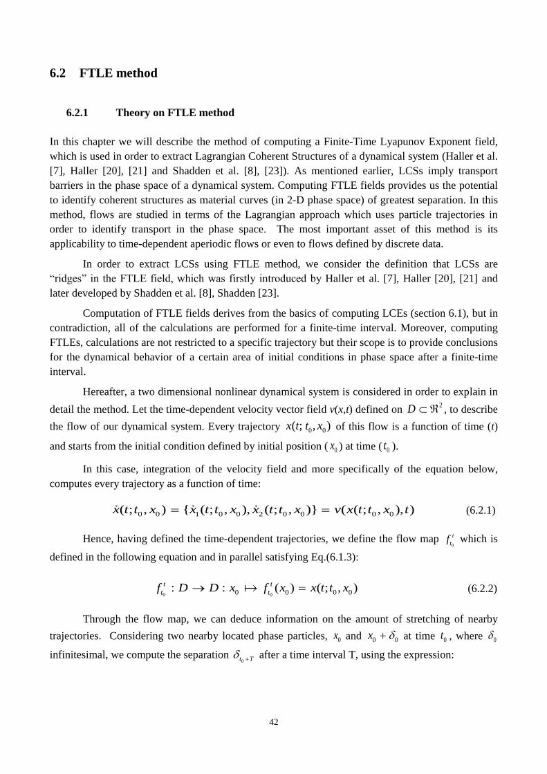
6.2 FTLE method

6.2.1 Theory on FTLE method

In this chapter we will describe the method of computing a Finite-Time Lyapunov Exponent field,

which is used in order to extract Lagrangian Coherent Structures of a dynamical system (Haller et al.

[7], Haller [20], [21] and Shadden et al. [8], [23]). As mentioned earlier, LCSs imply transport

barriers in the phase space of a dynamical system. Computing FTLE fields provides us the potential

to identify coherent structures as material curves (in 2-D phase space) of greatest separation. In this

method, flows are studied in terms of the Lagrangian approach which uses particle trajectories in

order to identify transport in the phase space. The most important asset of this method is its

applicability to time-dependent aperiodic flows or even to flows defined by discrete data.

In order to extract LCSs using FTLE method, we consider the definition that LCSs are

“ridges” in the FTLE field, which was firstly introduced by Haller et al. [7], Haller [20], [21] and

later developed by Shadden et al. [8], Shadden [23].

Computation of FTLE fields derives from the basics of computing LCEs (section 6.1), but in

contradiction, all of the calculations are performed for a finite-time interval. Moreover, computing

FTLEs, calculations are not restricted to a specific trajectory but their scope is to provide conclusions

for the dynamical behavior of a certain area of initial conditions in phase space after a finite-time

interval.

Hereafter, a two dimensional nonlinear dynamical system is considered in order to explain in

detail the method. Let the time-dependent velocity vector field v(x,t) defined on 2D , to describe

the flow of our dynamical system. Every trajectory 0 0( ; , )x t t x of this flow is a function of time (t)

and starts from the initial condition defined by initial position ( 0x ) at time ( 0t ).

In this case, integration of the velocity field and more specifically of the equation below,

computes every trajectory as a function of time:

0 0 1 0 0 2 0 0 0 0( ; , ) { ( ; , ), ( ; , )} ( ( ; , ), )x t t x x t t x x t t x v x t t x t (6.2.1)

Hence, having defined the time-dependent trajectories, we define the flow map 0

t

tf which is

defined in the following equation and in parallel satisfying Eq.(6.1.3):

0 00 0 0 0: : ( ) ( ; , )t t

t tf D D x f x x t t x (6.2.2)

Through the flow map, we can deduce information on the amount of stretching of nearby

trajectories. Considering two nearby located phase particles, 0x and 0 0x at time 0t , where 0

infinitesimal, we compute the separation 0t T after a time interval T, using the expression:

43

0

00 0

0 0 0 0

2

0 0 0 0 0( ) ( ) |

t T

tt T t T

t T t t x x

ff x f x

x

(6.2.3)

0

0 0 0

t T

t T tDf

(6.2.4)

From theory it is known that linearization of the flow map, provides the linearized stretching t T

tDf (see also Shadden et al. [8]) for a finite interval of time T, which depicts the growth rate of a

set of vectors around the trajectory. Because of the two-dimensional dynamical system, t T

tDf is a

2x2 real matrix.

Let’s consider:

t T

t

a bDf

c d

(6.2.5)

The amount of the stretching is obtained by computing the (right) Cauchy-Green deformation

tensor (Shadden et al. [8]):

' [ ( )]' ( )t T t T

t tDf x Df x =[𝑎 𝑏𝑐 𝑑

] ∙ [𝑎 𝑐𝑏 𝑑

] = [𝑎2 + 𝑐2 𝑎𝑏 + 𝑐𝑑𝑎𝑏 + 𝑐𝑑 𝑏2 + 𝑑2 ] (6.2.6)

where A’ is the transposed form of matrix A.

So, considering now that 0

0

0

ˆ

is the vector in the direction of the initial separation.

Combining Eq. (6.2.4) and (6.2.6), the norm Eq. (6.2.4) is expressed as:

0 0 0

0 0 0 0

''

0 0 0 0ˆ ˆt T t T t T

t T t t tDf Df Df

(6.2.7)

From the expression (6.2.6) it is obvious that the deformation tensor Δ depends on the

variables x,t,,T. Moreover, it is deduced that Δ is assigned with each point of the flow map. It is also

noticed and proved below that Cauchy-Green deformation tensor has a positive definition.

Formal Algebra Definition: In linear algebra, a symmetric nxn real matrix M is said to be

positive definite if xTMx is positive for every non-zero column vector x of n real numbers. The

symmetric real matrix Δ=[𝑎2 + 𝑐2 𝑎𝑏 + 𝑐𝑑𝑎𝑏 + 𝑐𝑑 𝑏2 + 𝑑2] is positive definite since for any non-zero column

vector x =[𝑥𝑦], we have:

Q = xTMx = [x y] [

𝑎 𝑏𝑐 𝑑

] [𝑥𝑦] = [x (a

2+c

2) + y (ab+cd) x (ab+cd) + y (b

2+d

2)][

𝑥𝑦] =

= x2(a

2+c

2) + xy(ab+cd) + xy(ab+cd) + y

2(b

2+d

2) = x

2(a

2+c

2) + 2xy(ab+cd) + y

2(b

2+d

2) =

=x2a

2+ x

2c

2+2xyab+2xycd+y

2b

2+ y

2d

2 = (ax+by)

2 + (cx+dy)

2 >0

As a result Δ is positive definite and zero for a=b=c=d=0.

44

In order to measure the magnitude of stretching of the nearby particles of phase space, we

define the following limit (Shadden et al. [8]):

0 0 0

0 00

''

0 00

0

ˆ ˆlimt T t T t T

t tDf Df

(6.2.8)

The above proof leads to the conclusion that Δ has positive eigenvalues (λ1, λ2) that represent

the magnitude of stretching at each direction of the corresponding eigenvector. So, the magnitude of

stretching of two nearby particles in the i-th eigen-direction is:

0

0 00

lim ( )t T

i

(6.2.9)

where 0t T , 0 represent separation in the direction of the i-th eigenvector.

Now, considering the logarithm of Eq.(6.2.9) and dividing the term with the time interval T

so as to obtain the average value, we define the Finite-Time Lyapunov Exponent (Shadden et al. [8]):

1

( , ) : ln( ( ))i

T ix t

(6.2.10)

Subsequently, maximum stretching occurs in the direction of the eigenvectors associated with

the maximum eigenvalue (λmax) of the deformation tensor Δ. In practice, maximum eigenvalue

indicates the magnitude of the expansion along the direction of the corresponding eigenvector. So,

considering Eq.(6.2.7), maximum stretching of two nearby trajectories is expressed by the following

form:

0 0

0 0

( , )

0 max 0 0 0max ( ) max T x t Tt T t T

t tDf Df e

(6.2.11)

where δ0 is the initial separation in the direction of the eigenvector associated with the largest

eigenvalue (λmax(Δ)), ( )x is the largest Lyapunov Exponent computed for the time interval T and

also associated with the reference trajectory (initial condition: 0x at time 0t ).

Finally, for each phase particle of the flow map, we use λmax to compute FTLEs through the

following expression:

max

1( , ) : ln( ( ))x t

(6.2.12)

which is the function that represents the largest Finite-Time Lyapunov Exponent with a finite

integration of time T associated with point x at time t.

We also have to point out that:

if max0 1 , then max 0ln → 0

0T

t

if max 1 , then max 0ln → 0

0T

t

45

Through the definition of Eq.(6.2.10), FTLE provides a measure of separation of nearby

trajectories advected by the flow over the interval of time (t, t+T). Through the aforementioned

method of computing FTLE field, recognition of local maximizing curves in the field provides us the

opportunity to recognize LCSs. According to Shadden et al. [8], local maximizing curves in 2-D

phase space, are “ridge curves”, which implies that in the transverse region of the tangent to that

curve direction, only lower FTLEs are obtained.

Implementation of the method for negative integration time T implies separation backward in

time which means convergence in forward time. Haller et al. [7] proposed that attracting Lagrangian

Coherent Structures are revealed using backward-time integration and repelling Lagrangian Coherent

Structures are revealed using forward-time integration. LCSs in the phase space of a 2-Dimensional

dynamical system, separate regions of different dynamical behavior by acting as barriers of the flow

transport. Attracting LCSs tend to attract neighbor trajectories and repelling LCSs tend to repel

nearby trajectories towards attracting LCSs. In that way, frameworks delineated by LCSs are

structured comparable to that created by stable and unstable manifolds. Furthermore, intersections of

attracting and repelling LCSs are comparable to saddle points.

The choice of the integration time T is crucial. Choosing low value of T wouldn’t reveal all

the LCSs in the FTLE field. Furthermore, increasing T makes the ridges of the FTLE field sharper.

However, very large integration time T may result poor depiction of certain parts of LCSs that could

be revealed using smaller time interval. So, the value of the integration time T should be sufficient

for all LCSs to be revealed.

6.2.2 Computation of the FTLE method in surge motion equation

In this section we attempt to make a brief description of the computational method implemented in

order to extract LCSs. Although the theoretical approach of the method is already presented in

section 6.2.1, it is necessary to explain the computational steps in more detail.

In the analysis of the basics of FTLE method, according to Shadden et al. [8], we consider a

two-dimensional time-dependent dynamical system, which is described by ship’s surge equation

(Eq.4.9) and corresponds to a flow in phase space2D . Depending on the wave excitation

(regular, bi-chromatic or irregular), we choose the appropriate wave excitation term in surge

equation, which is going to be integrated forward and backward in time.

Hence, we firstly define a flow map which gives the new position of an initial condition

0 0,x u at time 0t , after a time interval T ( 0T t t ). We then construct a grid of NxN initial

conditions 20 0 1...,

i Nx u

in phase space at time 0t scattered uniformly in phase-plane. In this phase

space horizontal axis corresponds to position x(t) and vertical axis corresponds to velocity'( )u x t .

Hereafter, the FTLE field that we are going to calculate is delineated in the region of2D . It is

apparent that increasing the number of the grid points, we gain the advantage of better quality of the

FTLE field due to the large density of the grid, but on the other hand the computational time needed

46

for integration in order to compute the new point positions and also the FTLE values is also

increasing, which practically constitutes an important disadvantage.

Afterwards, we continue with the integration of the scheme of initial conditions described

before, with regard to the dynamical system of surge motions equation. Integrating numerically each

one point in the grid for a time interval T, incurs the construction of a new grid containing the new

point positions 0 0 0 0 0 0{ ( ; , ), '( ; , )}x t T t x x t T t x .

Continuing, estimation of the deformation tensor Δ asserts the construction of a finite

difference scheme at each point of the grid, considering its initial as well as its new position after

time T. Having calculated the deformation tensor for each point of the grid separately, we now

compute the eigenvalues of each one tensor, and then keep the largest one. Inserting maximum

eigenvalues in Eq. (6.2.12), we compute the FTLE value for each grid point. Subsequently, the FTLE

scalar field is provided. In other words, by associating each initial point in the grid with the largest

FTLE, a scalar field is obtained for a specific instance in time.

By choosing to show only the largest FTLEs in the field, the identification of LCSs is

provided. Practically, integration of the grid forward in time provides the identification of repelling

LCSs and in parallel backward in time integration reveals the attracting LCSs which are comparable

to finite-time stable and unstable manifolds respectively.

Repeating the calculation of the FTLE field for a time series we obtain the evolution of

attracting and repelling LCSs in time. This approach is considered quite interesting for irregular

wave excitation.

47

6.3 FSLE method

In this section we will make a brief description of the Finite-Size Lyapunov Exponents’ (FSLE)

method so as to point out its relation with the FTLE method, already described in Section 6.2 of this

chapter. Although the aforementioned method has many similarities with the FTLE method while it

constitutes another method of computing hyperbolic LCSs, we did not consider as necessary to

implement an FSLE calculation method in the context of this thesis.

In order to describe the method we firstly consider a dynamical system in phase space and in

parallel we create a grid of initial conditions as described in section 6.2. In the case of FSLE method,

we consider the initial separation of particles from position x in phase space, at time t, to be

0( , ,0)d x t d , as well as a factor (r) representing the growth of the separation after the time interval

T. Having defined these parameters we use the below expression in order to calculate the FSLE:

0

ln( , , )r

rx t d

(6.3.1)

In the above expression, T is the interval of time after which the separation will be

0( , , )d x t T rd . Roughly speaking, in the FSLE method we have to define a specific separation of

particles from an initial position x in phase space, defining the growth factor r. For cases that at time

t+T separation reaches this value, we compute FSLE’s value. In cases that separation never reaches

this value, we set zero FSLE value. Hence, T is the interval of time needed so as to obtain separation

in phase space multiplied by a factor r.

Similarly to the FTLE calculation method, in cases of 1r , by plotting the maximum

FSLE values for forward in time integration we capture repelling LCSs; while through backward in

time integration, the attracting LCSs are provided. Visualization of the LCSs is attained by plotting

the FSLE values in a map designated by a grid containing the initial positions of particles in phase

space.

48

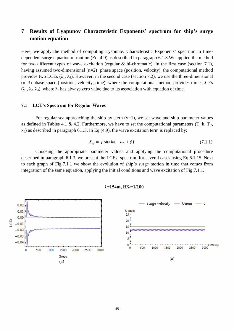
49

7 Results of Lyapunov Characteristic Exponents’ spectrum for ship’s surge

motion equation

Here, we apply the method of computing Lyapunov Characteristic Exponents’ spectrum in time-

dependent surge equation of motion (Eq. 4.9) as described in paragraph 6.1.3.We applied the method

for two different types of wave excitation (regular & bi-chromatic). In the first case (section 7.1),

having assumed two-dimensional (n=2) phase space (position, velocity), the computational method

provides two LCEs (λ1, λ2). However, in the second case (section 7.2), we use the three-dimensional

(n=3) phase space (position, velocity, time), where the computational method provides three LCEs

(λ1, λ2, λ3). where λ3 has always zero value due to its association with equation of time.

7.1 LCE’s Spectrum for Regular Waves

For regular sea approaching the ship by stern (v=1), we set wave and ship parameter values

as defined in Tables 4.1 & 4.2. Furthermore, we have to set the computational parameters (T, k, TR,

x0) as described in paragraph 6.1.3. In Eq.(4.9), the wave excitation term is replaced by:

sin( )wX f kx t (7.1.1)

Choosing the appropriate parameter values and applying the computational procedure

described in paragraph 6.1.3, we present the LCEs’ spectrum for several cases using Eq.6.1.15. Next

to each graph of Fig.7.1.1 we show the evolution of ship’s surge motion in time that comes from

integration of the same equation, applying the initial conditions and wave excitation of Fig.7.1.1.

λ=154m, H/λ=1/100

(a)

(a)

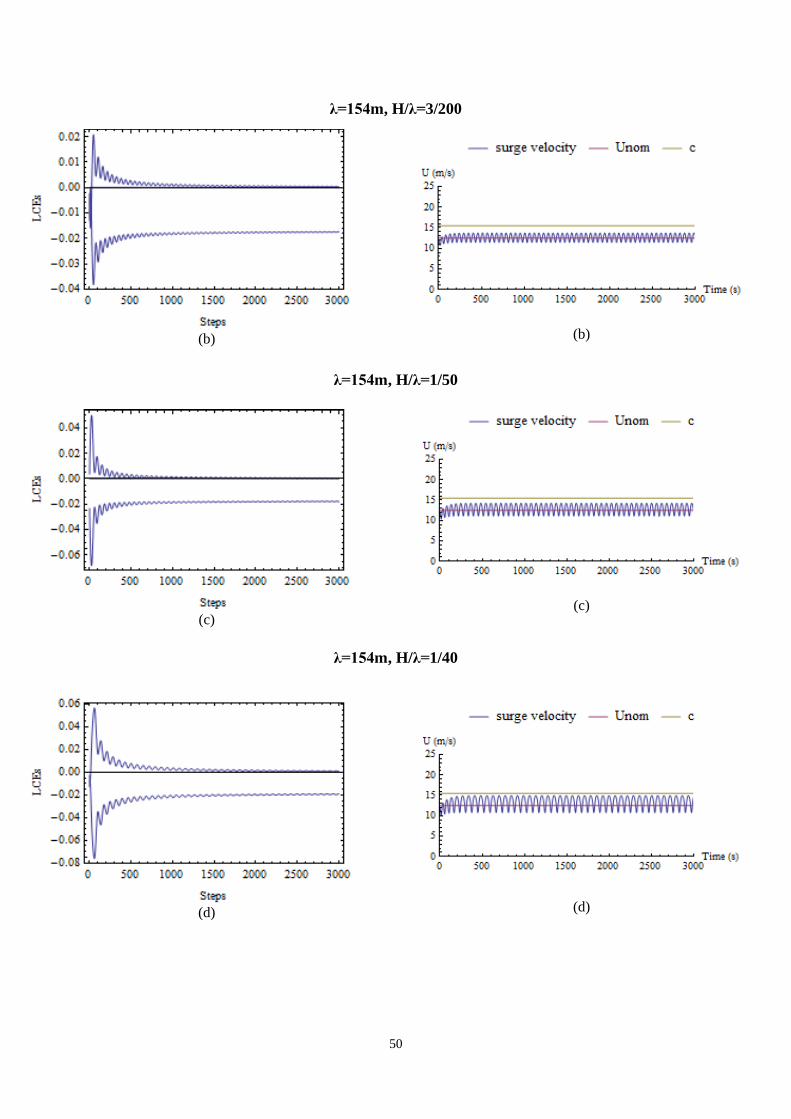
50

λ=154m, H/λ=3/200

(b)

(b)

λ=154m, H/λ=1/50

(c)

(c)

λ=154m, H/λ=1/40

(d)

(d)

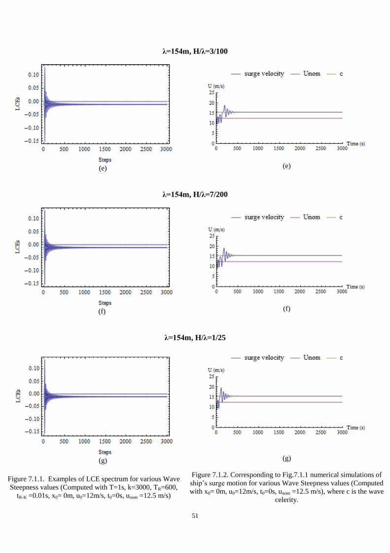
51

λ=154m, H/λ=3/100

(e)

(e)

λ=154m, H/λ=7/200

(f)

(f)

λ=154m, H/λ=1/25

(g)

(g)

Figure 7.1.1. Examples of LCE spectrum for various Wave

Steepness values (Computed with T=1s, k=3000, TR=600,

tR-K =0.01s, x0= 0m, u0=12m/s, t0=0s, unom =12.5 m/s)

Figure 7.1.2. Corresponding to Fig.7.1.1 numerical simulations of

ship’s surge motion for various Wave Steepness values (Computed

with x0= 0m, u0=12m/s, t0=0s, unom =12.5 m/s), where c is the wave

celerity.

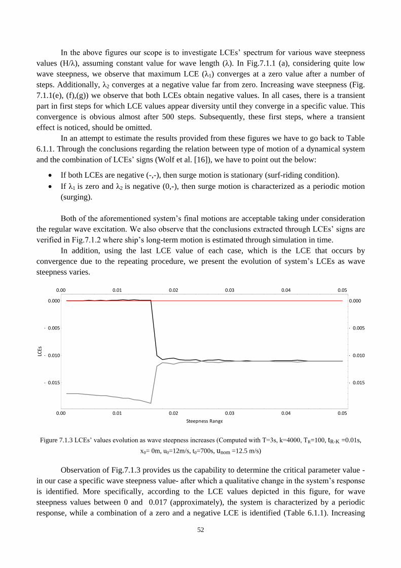
52

In the above figures our scope is to investigate LCEs’ spectrum for various wave steepness

values (H/λ), assuming constant value for wave length (λ). In Fig.7.1.1 (a), considering quite low

wave steepness, we observe that maximum LCE (λ1) converges at a zero value after a number of

steps. Additionally, λ2 converges at a negative value far from zero. Increasing wave steepness (Fig.

7.1.1(e), (f),(g)) we observe that both LCEs obtain negative values. In all cases, there is a transient

part in first steps for which LCE values appear diversity until they converge in a specific value. This

convergence is obvious almost after 500 steps. Subsequently, these first steps, where a transient

effect is noticed, should be omitted.

In an attempt to estimate the results provided from these figures we have to go back to Table

6.1.1. Through the conclusions regarding the relation between type of motion of a dynamical system

and the combination of LCEs’ signs (Wolf et al. [16]), we have to point out the below:

If both LCEs are negative (-,-), then surge motion is stationary (surf-riding condition).

If λ1 is zero and λ2 is negative (0,-), then surge motion is characterized as a periodic motion

(surging).

Both of the aforementioned system’s final motions are acceptable taking under consideration

the regular wave excitation. We also observe that the conclusions extracted through LCEs’ signs are

verified in Fig.7.1.2 where ship’s long-term motion is estimated through simulation in time.

In addition, using the last LCE value of each case, which is the LCE that occurs by

convergence due to the repeating procedure, we present the evolution of system’s LCEs as wave

steepness varies.

Figure 7.1.3 LCEs’ values evolution as wave steepness increases (Computed with T=3s, k=4000, TR=100, tR-K =0.01s,

x0= 0m, u0=12m/s, t0=700s, unom =12.5 m/s)

Observation of Fig.7.1.3 provides us the capability to determine the critical parameter value -

in our case a specific wave steepness value- after which a qualitative change in the system’s response

is identified. More specifically, according to the LCE values depicted in this figure, for wave

steepness values between 0 and 0.017 (approximately), the system is characterized by a periodic

response, while a combination of a zero and a negative LCE is identified (Table 6.1.1). Increasing

0.00 0.01 0.02 0.03 0.04 0.05

0.015

0.010

0.005

0.000

0.00 0.01 0.02 0.03 0.04 0.05

0.015

0.010

0.005

0.000

Steepness Range

LCEs

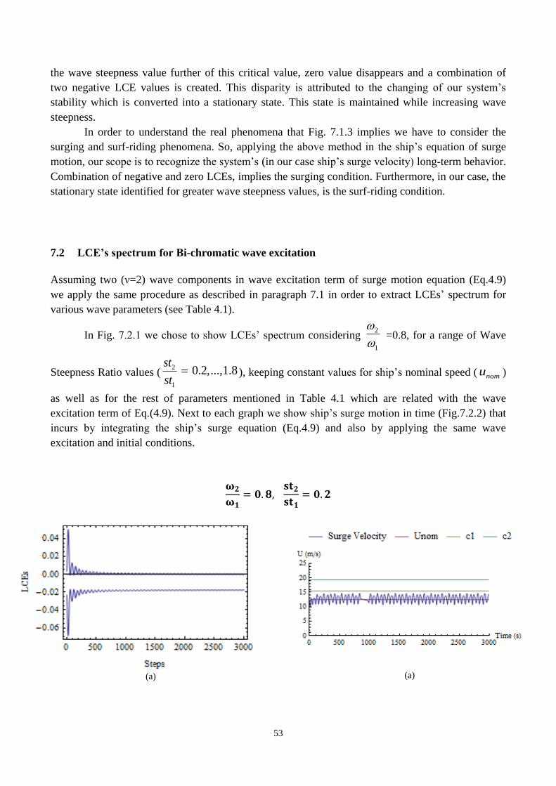
53

the wave steepness value further of this critical value, zero value disappears and a combination of

two negative LCE values is created. This disparity is attributed to the changing of our system’s

stability which is converted into a stationary state. This state is maintained while increasing wave

steepness.

In order to understand the real phenomena that Fig. 7.1.3 implies we have to consider the

surging and surf-riding phenomena. So, applying the above method in the ship’s equation of surge

motion, our scope is to recognize the system’s (in our case ship’s surge velocity) long-term behavior.

Combination of negative and zero LCEs, implies the surging condition. Furthermore, in our case, the

stationary state identified for greater wave steepness values, is the surf-riding condition.

7.2 LCE’s spectrum for Βi-chromatic wave excitation

Assuming two (ν=2) wave components in wave excitation term of surge motion equation (Eq.4.9)

we apply the same procedure as described in paragraph 7.1 in order to extract LCEs’ spectrum for

various wave parameters (see Table 4.1).

In Fig. 7.2.1 we chose to show LCEs’ spectrum considering 2

1

=0.8, for a range of Wave

Steepness Ratio values (2

1

0.2,...,1.8st

st ), keeping constant values for ship’s nominal speed ( nomu )

as well as for the rest of parameters mentioned in Table 4.1 which are related with the wave

excitation term of Eq.(4.9). Next to each graph we show ship’s surge motion in time (Fig.7.2.2) that

incurs by integrating the ship’s surge equation (Eq.4.9) and also by applying the same wave

excitation and initial conditions.

𝛚𝟐

𝛚𝟏= 𝟎. 𝟖,

𝐬𝐭𝟐

𝐬𝐭𝟏= 𝟎. 𝟐

(a)

(a)

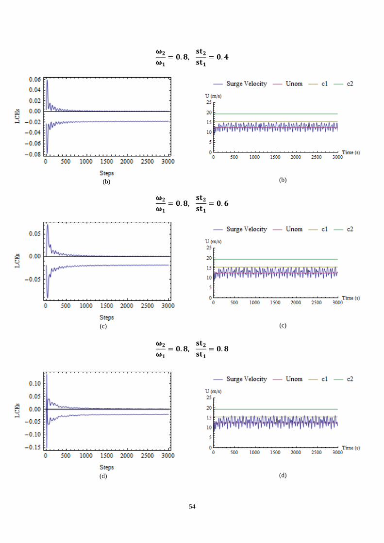
54

𝛚𝟐

𝛚𝟏= 𝟎. 𝟖,

𝐬𝐭𝟐

𝐬𝐭𝟏= 𝟎. 𝟒

(b)

(b)

𝛚𝟐

𝛚𝟏= 𝟎. 𝟖,

𝐬𝐭𝟐

𝐬𝐭𝟏= 𝟎. 𝟔

(c)

(c)

𝛚𝟐

𝛚𝟏= 𝟎. 𝟖,

𝐬𝐭𝟐

𝐬𝐭𝟏= 𝟎. 𝟖

(d)

(d)

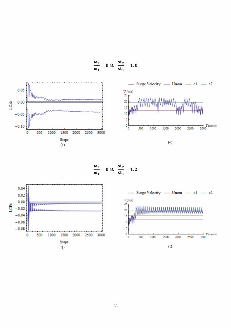
55

𝛚𝟐

𝛚𝟏= 𝟎. 𝟖,

𝐬𝐭𝟐

𝐬𝐭𝟏= 𝟏. 𝟎

(e)

(e)

𝛚𝟐

𝛚𝟏= 𝟎. 𝟖,

𝐬𝐭𝟐

𝐬𝐭𝟏= 𝟏. 𝟐

(f)

(f)

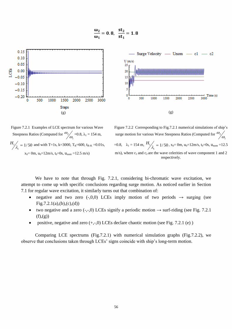
56

𝛚𝟐

𝛚𝟏= 𝟎. 𝟖,

𝐬𝐭𝟐

𝐬𝐭𝟏= 𝟏. 𝟖

(g)

(g)

Figure 7.2.1 Examples of LCE spectrum for various Wave

Steepness Ratios (Computed for 2

1

=0.8, λ1 = 154 m,

1

1

1/ 50H

and with T=1s, k=3000, TR=600, tR-K =0.01s,

x0= 0m, u0=12m/s, t0=0s, unom =12.5 m/s)

Figure 7.2.2 Corresponding to Fig.7.2.1 numerical simulations of ship’s

surge motion for various Wave Steepness Ratios (Computed for 2

1

=0.8, λ1 = 154 m, 1

1

1/ 50H

, x0= 0m, u0=12m/s, t0=0s, unom =12.5

m/s), where c1 and c2 are the wave celerities of wave component 1 and 2

respectively.

We have to note that through Fig. 7.2.1, considering bi-chromatic wave excitation, we

attempt to come up with specific conclusions regarding surge motion. As noticed earlier in Section

7.1 for regular wave excitation, it similarly turns out that combination of:

negative and two zero (-,0,0) LCEs imply motion of two periods → surging (see

Fig.7.2.1(a),(b),(c),(d))

two negative and a zero (-,-,0) LCEs signify a periodic motion → surf-riding (see Fig. 7.2.1

(f),(g))

positive, negative and zero (+,-,0) LCEs declare chaotic motion (see Fig. 7.2.1 (e) )

Comparing LCE spectrums (Fig.7.2.1) with numerical simulation graphs (Fig.7.2.2), we

observe that conclusions taken through LCEs’ signs coincide with ship’s long-term motion.

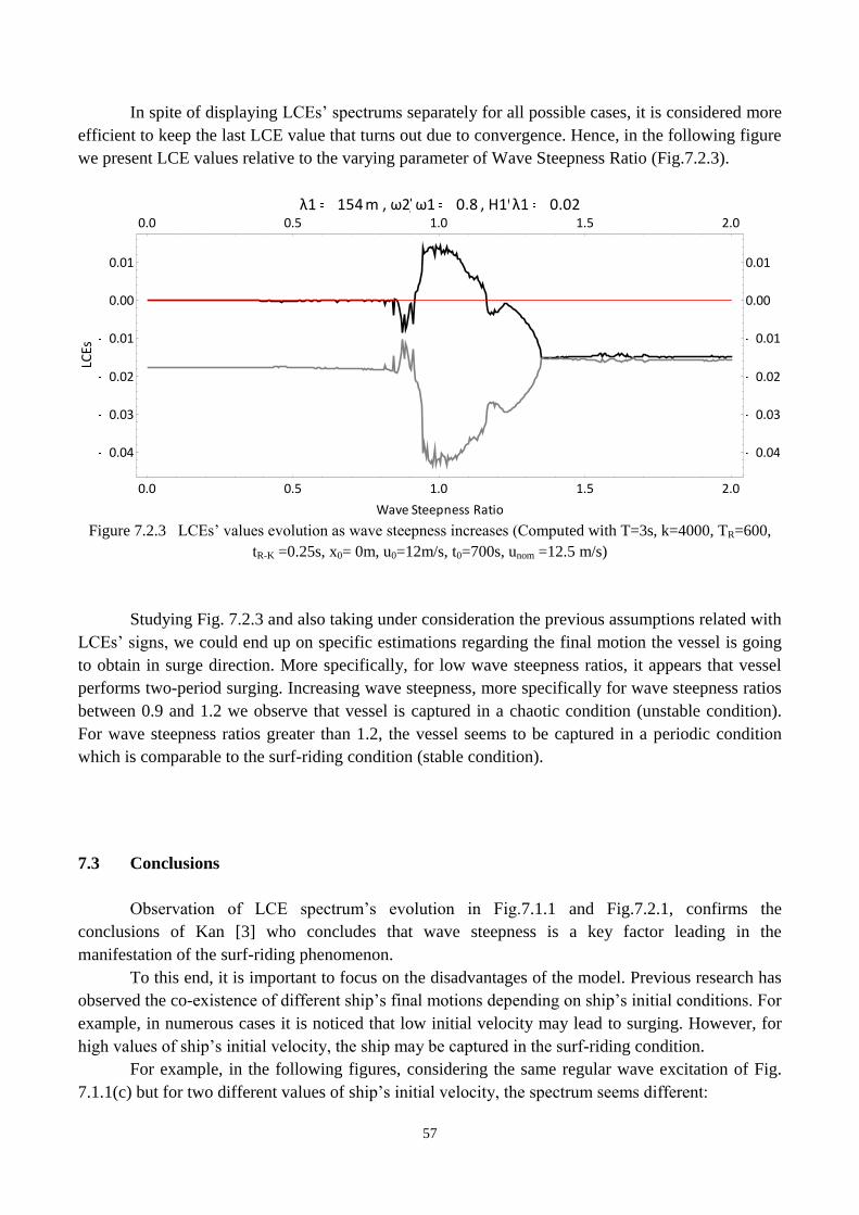
57

In spite of displaying LCEs’ spectrums separately for all possible cases, it is considered more

efficient to keep the last LCE value that turns out due to convergence. Hence, in the following figure

we present LCE values relative to the varying parameter of Wave Steepness Ratio (Fig.7.2.3).

Figure 7.2.3 LCEs’ values evolution as wave steepness increases (Computed with T=3s, k=4000, TR=600,

tR-K =0.25s, x0= 0m, u0=12m/s, t0=700s, unom =12.5 m/s)

Studying Fig. 7.2.3 and also taking under consideration the previous assumptions related with

LCEs’ signs, we could end up on specific estimations regarding the final motion the vessel is going

to obtain in surge direction. More specifically, for low wave steepness ratios, it appears that vessel

performs two-period surging. Increasing wave steepness, more specifically for wave steepness ratios

between 0.9 and 1.2 we observe that vessel is captured in a chaotic condition (unstable condition).

For wave steepness ratios greater than 1.2, the vessel seems to be captured in a periodic condition

which is comparable to the surf-riding condition (stable condition).

7.3 Conclusions

Observation of LCE spectrum’s evolution in Fig.7.1.1 and Fig.7.2.1, confirms the

conclusions of Kan [3] who concludes that wave steepness is a key factor leading in the

manifestation of the surf-riding phenomenon.

To this end, it is important to focus on the disadvantages of the model. Previous research has

observed the co-existence of different ship’s final motions depending on ship’s initial conditions. For

example, in numerous cases it is noticed that low initial velocity may lead to surging. However, for

high values of ship’s initial velocity, the ship may be captured in the surf-riding condition.

For example, in the following figures, considering the same regular wave excitation of Fig.

7.1.1(c) but for two different values of ship’s initial velocity, the spectrum seems different:

0.0 0.5 1.0 1.5 2.0

0.04

0.03

0.02

0.01

0.00

0.01

0.0 0.5 1.0 1.5 2.0

0.04

0.03

0.02

0.01

0.00

0.01

Wave Steepness Ratio

LCEs

λ1 154m , ω2 ω1 0.8 , Η1 λ1 0.02

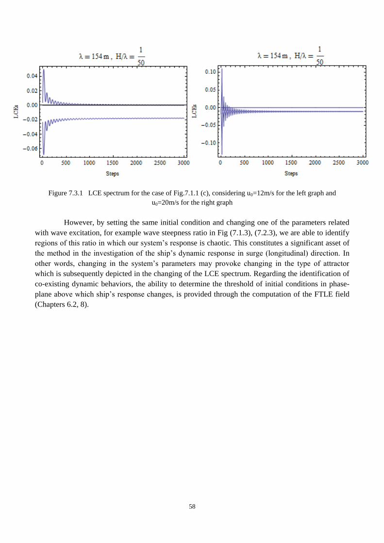
58

Figure 7.3.1 LCE spectrum for the case of Fig.7.1.1 (c), considering u0=12m/s for the left graph and

u0=20m/s for the right graph

However, by setting the same initial condition and changing one of the parameters related

with wave excitation, for example wave steepness ratio in Fig (7.1.3), (7.2.3), we are able to identify

regions of this ratio in which our system’s response is chaotic. This constitutes a significant asset of

the method in the investigation of the ship’s dynamic response in surge (longitudinal) direction. In

other words, changing in the system’s parameters may provoke changing in the type of attractor

which is subsequently depicted in the changing of the LCE spectrum. Regarding the identification of

co-existing dynamic behaviors, the ability to determine the threshold of initial conditions in phase-

plane above which ship’s response changes, is provided through the computation of the FTLE field

(Chapters 6.2, 8).

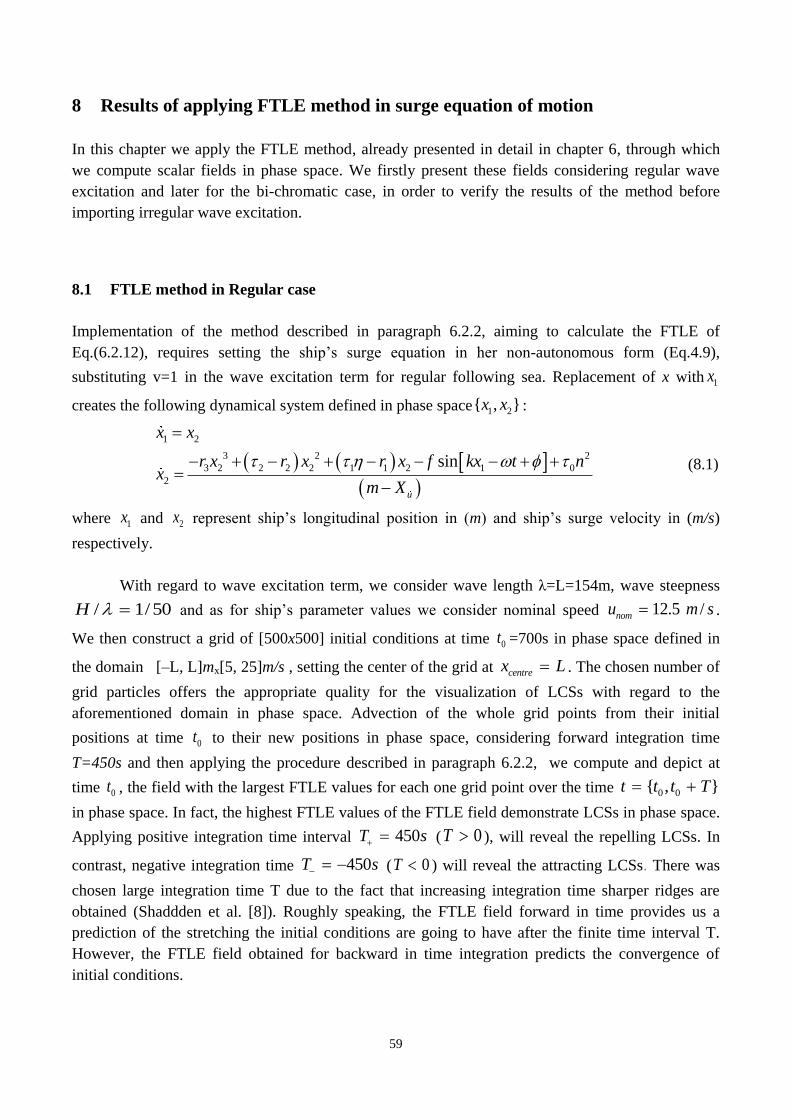
59

8 Results of applying FTLE method in surge equation of motion

In this chapter we apply the FTLE method, already presented in detail in chapter 6, through which

we compute scalar fields in phase space. We firstly present these fields considering regular wave

excitation and later for the bi-chromatic case, in order to verify the results of the method before

importing irregular wave excitation.

8.1 FTLE method in Regular case

Implementation of the method described in paragraph 6.2.2, aiming to calculate the FTLE of

Eq.(6.2.12), requires setting the ship’s surge equation in her non-autonomous form (Eq.4.9),

substituting v=1 in the wave excitation term for regular following sea. Replacement of x with 1x

creates the following dynamical system defined in phase space 1 2{ , }x x :

3 2 2

3

1 2

2 2 2 2 1 1 2 0

2

1sin   

u

r r x r x f k t nx

m X

x x

x x

(8.1)

where 1x and 2x represent ship’s longitudinal position in (m) and ship’s surge velocity in (m/s)

respectively.

With regard to wave excitation term, we consider wave length λ=L=154m, wave steepness

/ 1/50H and as for ship’s parameter values we consider nominal speed 12.5 /nomu m s .

We then construct a grid of [500x500] initial conditions at time 0t =700s in phase space defined in

the domain [–L, L]mx[5, 25]m/s , setting the center of the grid at centrex L . The chosen number of

grid particles offers the appropriate quality for the visualization of LCSs with regard to the

aforementioned domain in phase space. Advection of the whole grid points from their initial

positions at time 0t to their new positions in phase space, considering forward integration time

T=450s and then applying the procedure described in paragraph 6.2.2, we compute and depict at

time 0t , the field with the largest FTLE values for each one grid point over the time 0 0{ , }t t t T

in phase space. In fact, the highest FTLE values of the FTLE field demonstrate LCSs in phase space.

Applying positive integration time interval 450T s ( 0T ), will reveal the repelling LCSs. In

contrast, negative integration time 450T s ( 0T ) will reveal the attracting LCSs. There was

chosen large integration time T due to the fact that increasing integration time sharper ridges are

obtained (Shaddden et al. [8]). Roughly speaking, the FTLE field forward in time provides us a

prediction of the stretching the initial conditions are going to have after the finite time interval T.

However, the FTLE field obtained for backward in time integration predicts the convergence of

initial conditions.

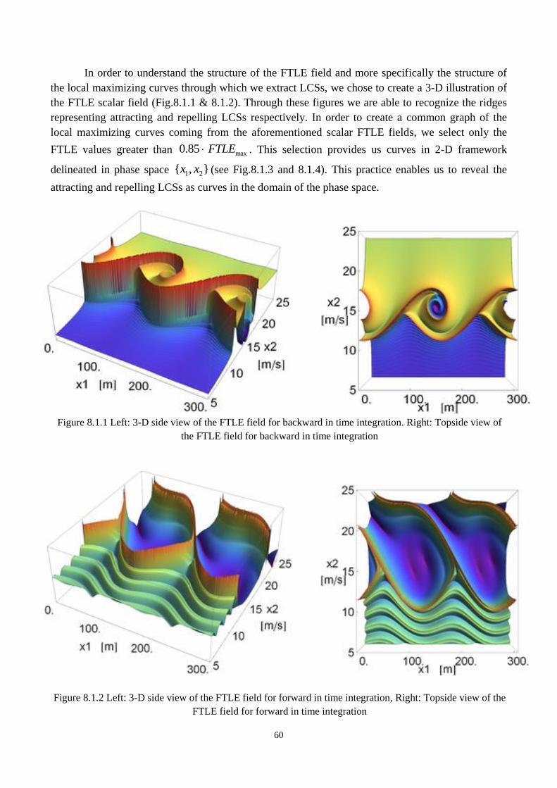
60

In order to understand the structure of the FTLE field and more specifically the structure of

the local maximizing curves through which we extract LCSs, we chose to create a 3-D illustration of

the FTLE scalar field (Fig.8.1.1 & 8.1.2). Through these figures we are able to recognize the ridges

representing attracting and repelling LCSs respectively. In order to create a common graph of the

local maximizing curves coming from the aforementioned scalar FTLE fields, we select only the

FTLE values greater than max0.85 FTLE . This selection provides us curves in 2-D framework

delineated in phase space 1 2{ , }x x (see Fig.8.1.3 and 8.1.4). This practice enables us to reveal the

attracting and repelling LCSs as curves in the domain of the phase space.

Figure 8.1.1 Left: 3-D side view of the FTLE field for backward in time integration. Right: Topside view of

the FTLE field for backward in time integration

Figure 8.1.2 Left: 3-D side view of the FTLE field for forward in time integration, Right: Topside view of the

FTLE field for forward in time integration

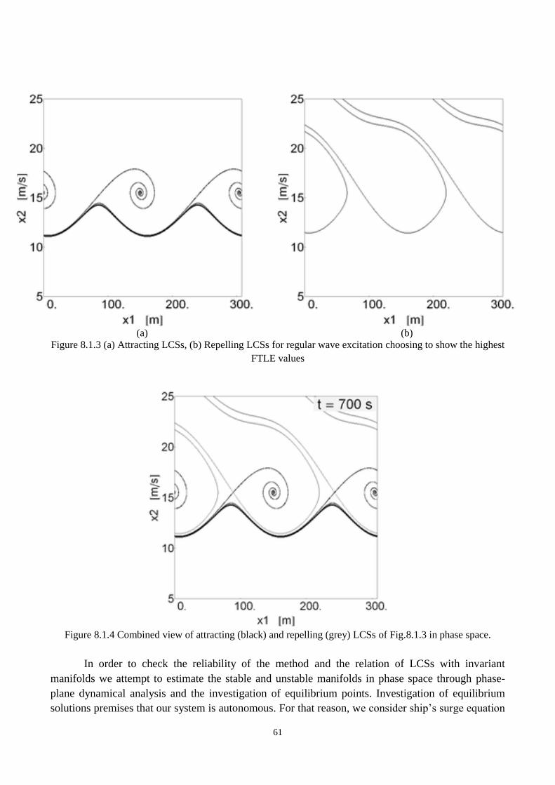
61

(a) (b)

Figure 8.1.3 (a) Attracting LCSs, (b) Repelling LCSs for regular wave excitation choosing to show the highest

FTLE values

Figure 8.1.4 Combined view of attracting (black) and repelling (grey) LCSs of Fig.8.1.3 in phase space.

In order to check the reliability of the method and the relation of LCSs with invariant

manifolds we attempt to estimate the stable and unstable manifolds in phase space through phase-

plane dynamical analysis and the investigation of equilibrium points. Investigation of equilibrium

solutions premises that our system is autonomous. For that reason, we consider ship’s surge equation

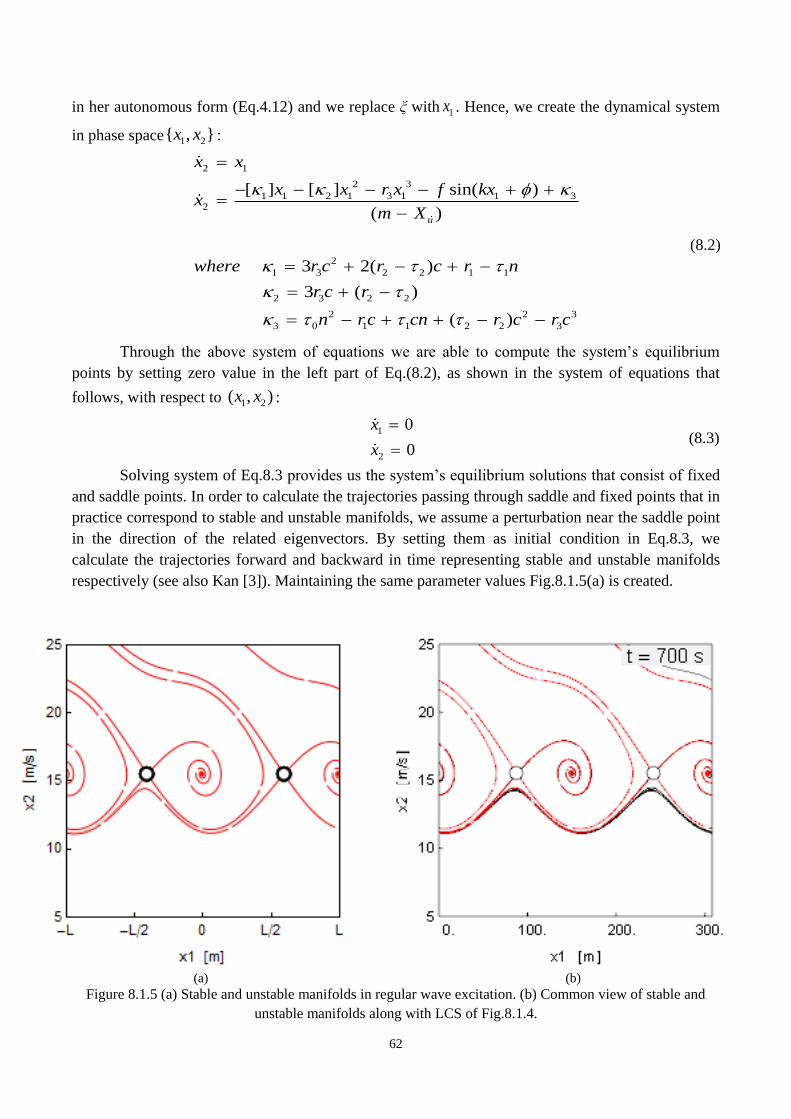
62

in her autonomous form (Eq.4.12) and we replace ξ with 1x . Hence, we create the dynamical system

in phase space 1 2{ , }x x :

2 1

2 3

1 1 2 1 3 1 1 32

2

1 3 2 2 1 1

2 3 2 2

2 2 3

3 0 1 1 2 2 3

[ ] [ ] sin( )

( )

3 2( )

3 ( )

( )

u

x x

x x r x f kxx

m X

where r c r c r n

r c r

n rc cn r c r c

(8.2)

Through the above system of equations we are able to compute the system’s equilibrium

points by setting zero value in the left part of Eq.(8.2), as shown in the system of equations that

follows, with respect to 1 2( , )x x :

1

2

0

0

x

x

(8.3)

Solving system of Eq.8.3 provides us the system’s equilibrium solutions that consist of fixed

and saddle points. In order to calculate the trajectories passing through saddle and fixed points that in

practice correspond to stable and unstable manifolds, we assume a perturbation near the saddle point

in the direction of the related eigenvectors. By setting them as initial condition in Eq.8.3, we

calculate the trajectories forward and backward in time representing stable and unstable manifolds

respectively (see also Kan [3]). Maintaining the same parameter values Fig.8.1.5(a) is created.

(a) (b)

Figure 8.1.5 (a) Stable and unstable manifolds in regular wave excitation. (b) Common view of stable and

unstable manifolds along with LCS of Fig.8.1.4.

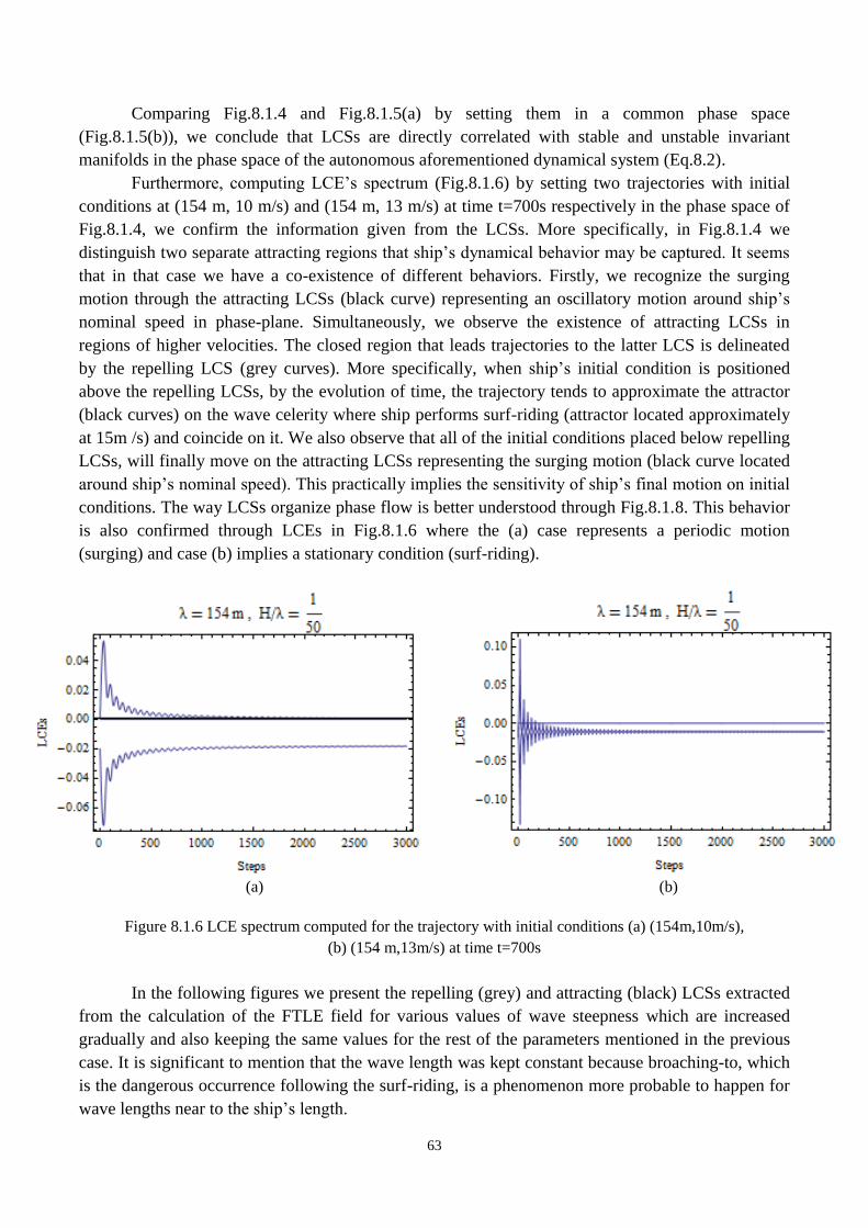
63

Comparing Fig.8.1.4 and Fig.8.1.5(a) by setting them in a common phase space

(Fig.8.1.5(b)), we conclude that LCSs are directly correlated with stable and unstable invariant

manifolds in the phase space of the autonomous aforementioned dynamical system (Eq.8.2).

Furthermore, computing LCE’s spectrum (Fig.8.1.6) by setting two trajectories with initial

conditions at (154 m, 10 m/s) and (154 m, 13 m/s) at time t=700s respectively in the phase space of

Fig.8.1.4, we confirm the information given from the LCSs. More specifically, in Fig.8.1.4 we

distinguish two separate attracting regions that ship’s dynamical behavior may be captured. It seems

that in that case we have a co-existence of different behaviors. Firstly, we recognize the surging

motion through the attracting LCSs (black curve) representing an oscillatory motion around ship’s

nominal speed in phase-plane. Simultaneously, we observe the existence of attracting LCSs in

regions of higher velocities. The closed region that leads trajectories to the latter LCS is delineated

by the repelling LCS (grey curves). More specifically, when ship’s initial condition is positioned

above the repelling LCSs, by the evolution of time, the trajectory tends to approximate the attractor

(black curves) on the wave celerity where ship performs surf-riding (attractor located approximately

at 15m /s) and coincide on it. We also observe that all of the initial conditions placed below repelling

LCSs, will finally move on the attracting LCSs representing the surging motion (black curve located

around ship’s nominal speed). This practically implies the sensitivity of ship’s final motion on initial

conditions. The way LCSs organize phase flow is better understood through Fig.8.1.8. This behavior

is also confirmed through LCEs in Fig.8.1.6 where the (a) case represents a periodic motion

(surging) and case (b) implies a stationary condition (surf-riding).

(a) (b)

Figure 8.1.6 LCE spectrum computed for the trajectory with initial conditions (a) (154m,10m/s),

(b) (154 m,13m/s) at time t=700s

In the following figures we present the repelling (grey) and attracting (black) LCSs extracted

from the calculation of the FTLE field for various values of wave steepness which are increased

gradually and also keeping the same values for the rest of the parameters mentioned in the previous

case. It is significant to mention that the wave length was kept constant because broaching-to, which

is the dangerous occurrence following the surf-riding, is a phenomenon more probable to happen for

wave lengths near to the ship’s length.

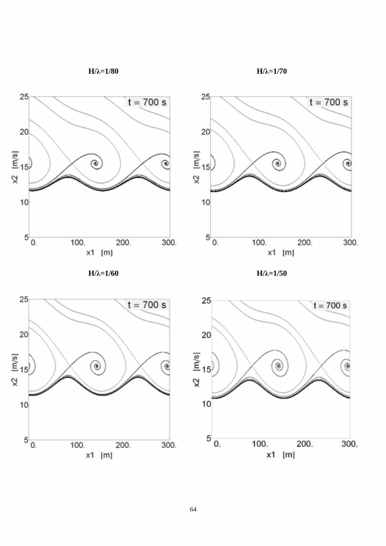
64

H/λ=1/80 H/λ=1/70

H/λ=1/60 H/λ=1/50

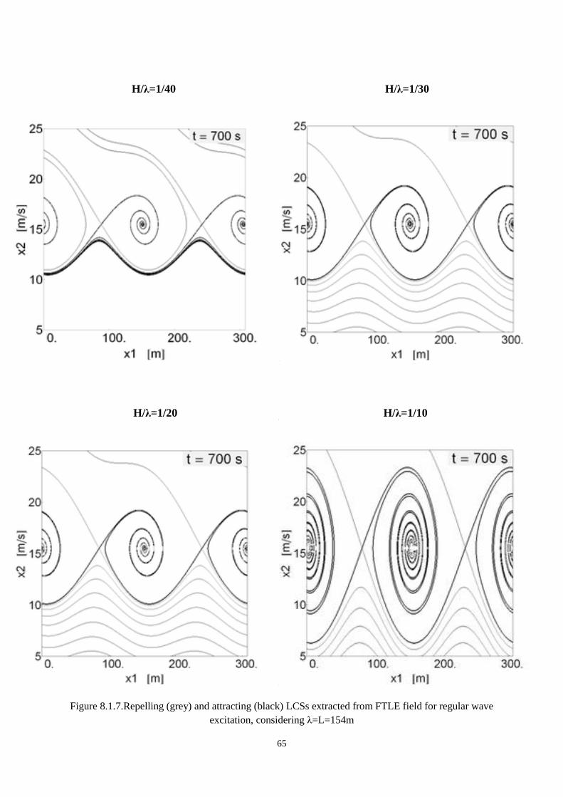
65

H/λ=1/40 H/λ=1/30

H/λ=1/20 H/λ=1/10

Figure 8.1.7.Repelling (grey) and attracting (black) LCSs extracted from FTLE field for regular wave

excitation, considering λ=L=154m

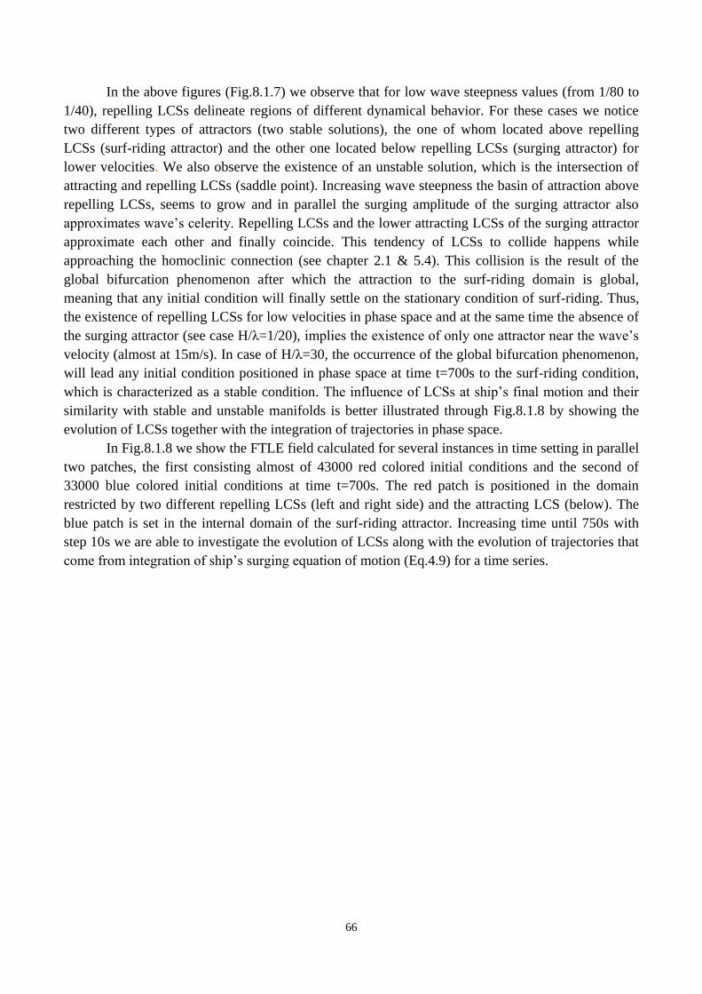
66

In the above figures (Fig.8.1.7) we observe that for low wave steepness values (from 1/80 to

1/40), repelling LCSs delineate regions of different dynamical behavior. For these cases we notice

two different types of attractors (two stable solutions), the one of whom located above repelling

LCSs (surf-riding attractor) and the other one located below repelling LCSs (surging attractor) for

lower velocities. We also observe the existence of an unstable solution, which is the intersection of

attracting and repelling LCSs (saddle point). Increasing wave steepness the basin of attraction above

repelling LCSs, seems to grow and in parallel the surging amplitude of the surging attractor also

approximates wave’s celerity. Repelling LCSs and the lower attracting LCSs of the surging attractor

approximate each other and finally coincide. This tendency of LCSs to collide happens while

approaching the homoclinic connection (see chapter 2.1 & 5.4). This collision is the result of the

global bifurcation phenomenon after which the attraction to the surf-riding domain is global,

meaning that any initial condition will finally settle on the stationary condition of surf-riding. Thus,

the existence of repelling LCSs for low velocities in phase space and at the same time the absence of

the surging attractor (see case H/λ=1/20), implies the existence of only one attractor near the wave’s

velocity (almost at 15m/s). In case of H/λ=30, the occurrence of the global bifurcation phenomenon,

will lead any initial condition positioned in phase space at time t=700s to the surf-riding condition,

which is characterized as a stable condition. The influence of LCSs at ship’s final motion and their

similarity with stable and unstable manifolds is better illustrated through Fig.8.1.8 by showing the

evolution of LCSs together with the integration of trajectories in phase space.

In Fig.8.1.8 we show the FTLE field calculated for several instances in time setting in parallel

two patches, the first consisting almost of 43000 red colored initial conditions and the second of

33000 blue colored initial conditions at time t=700s. The red patch is positioned in the domain

restricted by two different repelling LCSs (left and right side) and the attracting LCS (below). The

blue patch is set in the internal domain of the surf-riding attractor. Increasing time until 750s with

step 10s we are able to investigate the evolution of LCSs along with the evolution of trajectories that

come from integration of ship’s surging equation of motion (Eq.4.9) for a time series.

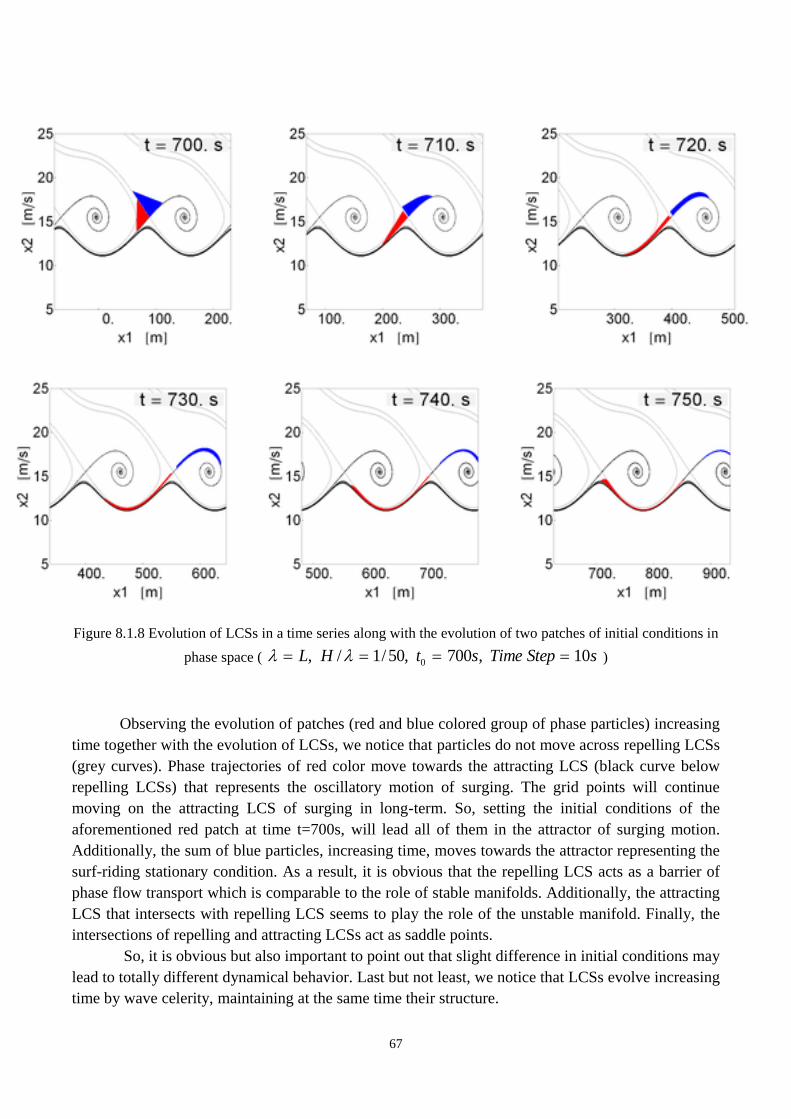
67

Figure 8.1.8 Evolution of LCSs in a time series along with the evolution of two patches of initial conditions in

phase space ( 0, / 1/ 50, 700 , 10L H t s Time Step s )

Observing the evolution of patches (red and blue colored group of phase particles) increasing

time together with the evolution of LCSs, we notice that particles do not move across repelling LCSs

(grey curves). Phase trajectories of red color move towards the attracting LCS (black curve below

repelling LCSs) that represents the oscillatory motion of surging. The grid points will continue

moving on the attracting LCS of surging in long-term. So, setting the initial conditions of the

aforementioned red patch at time t=700s, will lead all of them in the attractor of surging motion.

Additionally, the sum of blue particles, increasing time, moves towards the attractor representing the

surf-riding stationary condition. As a result, it is obvious that the repelling LCS acts as a barrier of

phase flow transport which is comparable to the role of stable manifolds. Additionally, the attracting

LCS that intersects with repelling LCS seems to play the role of the unstable manifold. Finally, the

intersections of repelling and attracting LCSs act as saddle points.

So, it is obvious but also important to point out that slight difference in initial conditions may

lead to totally different dynamical behavior. Last but not least, we notice that LCSs evolve increasing

time by wave celerity, maintaining at the same time their structure.

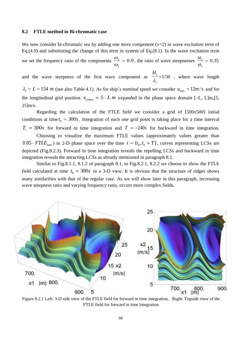
68

8.2 FTLE method in Βi-chromatic case

We now consider bi-chromatic sea by adding one more component (v=2) in wave excitation term of

Eq.(4.9) and substituting the change of this term in system of Eq.(8.1). In the wave excitation term

we set the frequency ratio of the components 2

1

0.9

, the ratio of wave steepnesses 2

1

0.35st

st

and the wave steepness of the first wave component as 1

1

H

=1/30 , where wave length

1 154L m (see also Table 4.1). As for ship’s nominal speed we consider 12 /nomu m s and for

the longitudinal grid position 5centrex L m expanded in the phase space domain [–L, L]mx[5,

25]m/s.

Regarding the calculation of the FTLE field we consider a grid of [500x500] initial

conditions at time 0 300t s . Integration of each one grid point is taking place for a time interval

300T s for forward in time integration and 240T s for backward in time integration.

Choosing to visualize the maximum FTLE values (approximately values greater than

max0.85 FTLE ) in 2-D phase space over the time 0 0{ , }t t t T , curves representing LCSs are

depicted (Fig.8.2.3). Forward in time integration reveals the repelling LCSs and backward in time

integration reveals the attracting LCSs as already mentioned in paragraph 8.1.

Similar to Fig.8.1.1, 8.1.2 of paragraph 8.1, in Fig.8.2.1, 8.2.2 we choose to show the FTLE

field calculated at time 0 300t s in a 3-D view. It is obvious that the structure of ridges shows

many similarities with that of the regular case. As we will show later in this paragraph, increasing

wave steepness ratio and varying frequency ratio, occurs more complex fields.

Figure 8.2.1 Left: 3-D side view of the FTLE field for forward in time integration, Right: Topside view of the

FTLE field for forward in time integration

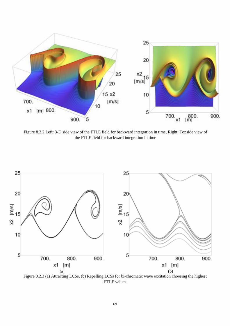
69

Figure 8.2.2 Left: 3-D side view of the FTLE field for backward integration in time, Right: Topside view of

the FTLE field for backward integration in time

(a) (b)

Figure 8.2.3 (a) Attracting LCSs, (b) Repelling LCSs for bi-chromatic wave excitation choosing the highest

FTLE values

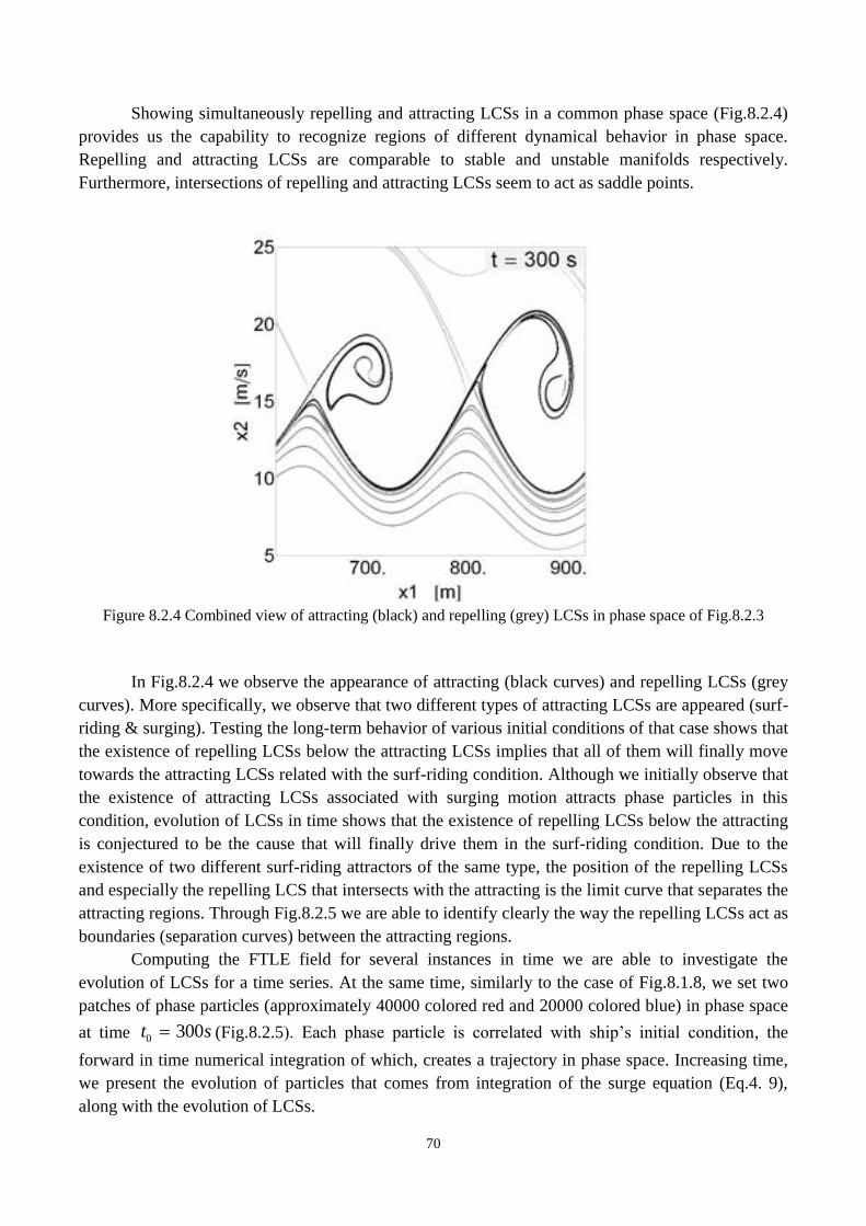
70

Showing simultaneously repelling and attracting LCSs in a common phase space (Fig.8.2.4)

provides us the capability to recognize regions of different dynamical behavior in phase space.

Repelling and attracting LCSs are comparable to stable and unstable manifolds respectively.

Furthermore, intersections of repelling and attracting LCSs seem to act as saddle points.

Figure 8.2.4 Combined view of attracting (black) and repelling (grey) LCSs in phase space of Fig.8.2.3

In Fig.8.2.4 we observe the appearance of attracting (black curves) and repelling LCSs (grey

curves). More specifically, we observe that two different types of attracting LCSs are appeared (surf-

riding & surging). Testing the long-term behavior of various initial conditions of that case shows that

the existence of repelling LCSs below the attracting LCSs implies that all of them will finally move

towards the attracting LCSs related with the surf-riding condition. Although we initially observe that

the existence of attracting LCSs associated with surging motion attracts phase particles in this

condition, evolution of LCSs in time shows that the existence of repelling LCSs below the attracting

is conjectured to be the cause that will finally drive them in the surf-riding condition. Due to the

existence of two different surf-riding attractors of the same type, the position of the repelling LCSs

and especially the repelling LCS that intersects with the attracting is the limit curve that separates the

attracting regions. Through Fig.8.2.5 we are able to identify clearly the way the repelling LCSs act as

boundaries (separation curves) between the attracting regions.

Computing the FTLE field for several instances in time we are able to investigate the

evolution of LCSs for a time series. At the same time, similarly to the case of Fig.8.1.8, we set two

patches of phase particles (approximately 40000 colored red and 20000 colored blue) in phase space

at time 0 300t s (Fig.8.2.5). Each phase particle is correlated with ship’s initial condition, the

forward in time numerical integration of which, creates a trajectory in phase space. Increasing time,

we present the evolution of particles that comes from integration of the surge equation (Eq.4. 9),

along with the evolution of LCSs.

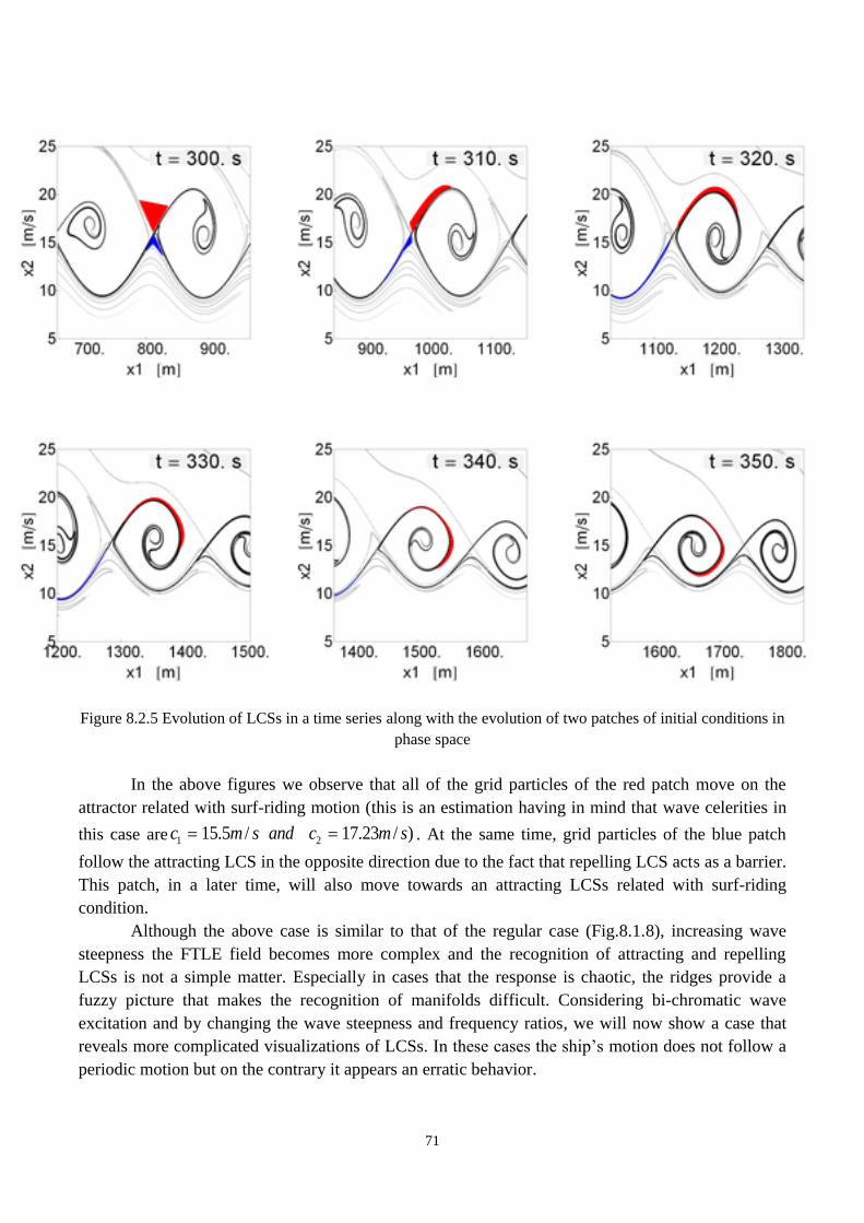
71

Figure 8.2.5 Evolution of LCSs in a time series along with the evolution of two patches of initial conditions in

phase space

In the above figures we observe that all of the grid particles of the red patch move on the

attractor related with surf-riding motion (this is an estimation having in mind that wave celerities in

this case are 1 215.5 / 17.23 / )c m s and c m s . At the same time, grid particles of the blue patch

follow the attracting LCS in the opposite direction due to the fact that repelling LCS acts as a barrier.

This patch, in a later time, will also move towards an attracting LCSs related with surf-riding

condition.

Although the above case is similar to that of the regular case (Fig.8.1.8), increasing wave

steepness the FTLE field becomes more complex and the recognition of attracting and repelling

LCSs is not a simple matter. Especially in cases that the response is chaotic, the ridges provide a

fuzzy picture that makes the recognition of manifolds difficult. Considering bi-chromatic wave

excitation and by changing the wave steepness and frequency ratios, we will now show a case that

reveals more complicated visualizations of LCSs. In these cases the ship’s motion does not follow a

periodic motion but on the contrary it appears an erratic behavior.

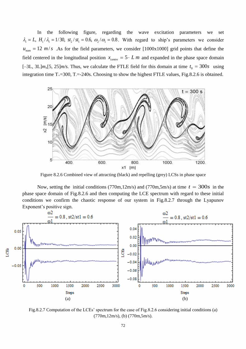
72

In the following figure, regarding the wave excitation parameters we set

1 1 1 2 1 2 1, / 1/30, / 0.6, / 0.8L H st st . With regard to ship’s parameters we consider

12 /nomu m s .As for the field parameters, we consider [1000x1000] grid points that define the

field centered in the longitudinal position 5centrex L m and expanded in the phase space domain

[–3L, 3L]mx[5, 25]m/s. Thus, we calculate the FTLE field for this domain at time 0 300t s using

integration time T+=300, T-=-240s. Choosing to show the highest FTLE values, Fig.8.2.6 is obtained.

Figure 8.2.6 Combined view of attracting (black) and repelling (grey) LCSs in phase space

Now, setting the initial conditions (770m,12m/s) and (770m,5m/s) at time 300t s in the

phase space domain of Fig.8.2.6 and then computing the LCE spectrum with regard to these initial

conditions we confirm the chaotic response of our system in Fig.8.2.7 through the Lyapunov

Exponent’s positive sign.

(a) (b)

Fig.8.2.7 Computation of the LCEs’ spectrum for the case of Fig.8.2.6 considering initial conditions (a)

(770m,12m/s), (b) (770m,5m/s).

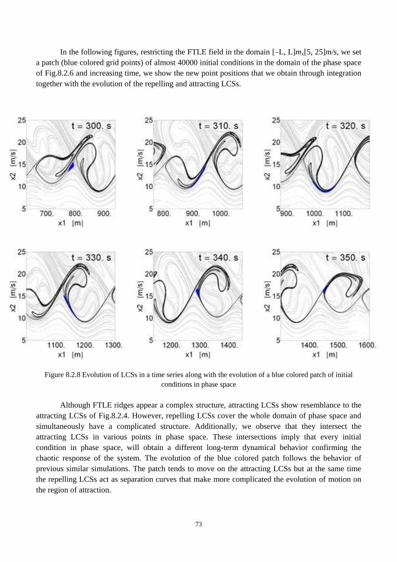
73

In the following figures, restricting the FTLE field in the domain [–L, L]mx[5, 25]m/s, we set

a patch (blue colored grid points) of almost 40000 initial conditions in the domain of the phase space

of Fig.8.2.6 and increasing time, we show the new point positions that we obtain through integration

together with the evolution of the repelling and attracting LCSs.

Figure 8.2.8 Evolution of LCSs in a time series along with the evolution of a blue colored patch of initial

conditions in phase space

Although FTLE ridges appear a complex structure, attracting LCSs show resemblance to the

attracting LCSs of Fig.8.2.4. However, repelling LCSs cover the whole domain of phase space and

simultaneously have a complicated structure. Additionally, we observe that they intersect the

attracting LCSs in various points in phase space. These intersections imply that every initial

condition in phase space, will obtain a different long-term dynamical behavior confirming the

chaotic response of the system. The evolution of the blue colored patch follows the behavior of

previous similar simulations. The patch tends to move on the attracting LCSs but at the same time

the repelling LCSs act as separation curves that make more complicated the evolution of motion on

the region of attraction.

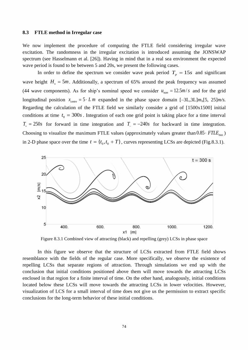
74

8.3 FTLE method in Irregular case

We now implement the procedure of computing the FTLE field considering irregular wave

excitation. The randomness in the irregular excitation is introduced assuming the JONSWAP

spectrum (see Hasselmann et al. [26]). Having in mind that in a real sea environment the expected

wave period is found to be between 5 and 20s, we present the following cases.

In order to define the spectrum we consider wave peak period 15pT s and significant

wave height 5sH m . Additionally, a spectrum of 65% around the peak frequency was assumed

(44 wave components). As for ship’s nominal speed we consider 12.5 /nomu m s and for the grid

longitudinal position 5centrex L m expanded in the phase space domain [–3L,3L]mx[5, 25]m/s.

Regarding the calculation of the FTLE field we similarly consider a grid of [1500x1500] initial

conditions at time 0 300t s . Integration of each one grid point is taking place for a time interval

250T s for forward in time integration and 240T s for backward in time integration.

Choosing to visualize the maximum FTLE values (approximately values greater than max0.85 FTLE )

in 2-D phase space over the time 0 0{ , }t t t T , curves representing LCSs are depicted (Fig.8.3.1).

Figure 8.3.1 Combined view of attracting (black) and repelling (grey) LCSs in phase space

In this figure we observe that the structure of LCSs extracted from FTLE field shows

resemblance with the fields of the regular case. More specifically, we observe the existence of

repelling LCSs that separate regions of attraction. Through simulations we end up with the

conclusion that initial conditions positioned above them will move towards the attracting LCSs

enclosed in that region for a finite interval of time. On the other hand, analogously, initial conditions

located below these LCSs will move towards the attracting LCSs in lower velocities. However,

visualization of LCS for a small interval of time does not give us the permission to extract specific

conclusions for the long-term behavior of these initial conditions.

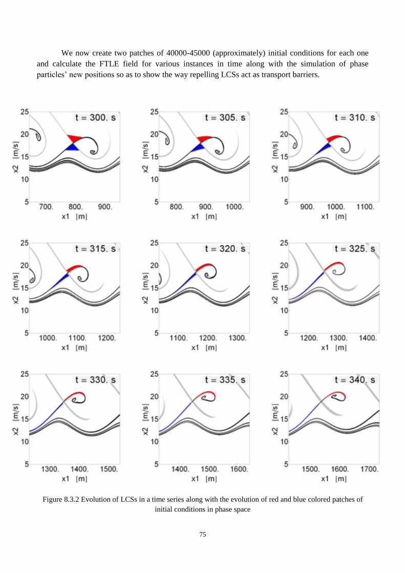
75

We now create two patches of 40000-45000 (approximately) initial conditions for each one

and calculate the FTLE field for various instances in time along with the simulation of phase

particles’ new positions so as to show the way repelling LCSs act as transport barriers.

Figure 8.3.2 Evolution of LCSs in a time series along with the evolution of red and blue colored patches of

initial conditions in phase space

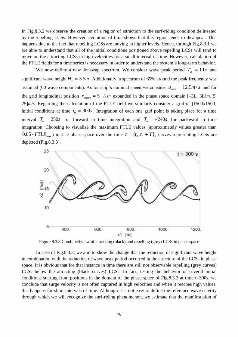
76

In Fig.8.3.2 we observe the creation of a region of attraction to the surf-riding condition delineated

by the repelling LCSs. However, evolution of time shows that this region tends to disappear. This

happens due to the fact that repelling LCSs are moving in higher levels. Hence, through Fig.8.3.1 we

are able to understand that all of the initial conditions positioned above repelling LCSs will tend to

move on the attracting LCSs in high velocities for a small interval of time. However, calculation of

the FTLE fields for a time series is necessary in order to understand the system’s long-term behavior.

We now define a new Jonswap spectrum. We consider wave peak period 11pT s and

significant wave height 3.5sH m . Additionally, a spectrum of 65% around the peak frequency was

assumed (60 wave components). As for ship’s nominal speed we consider 12.5 /nomu m s and for

the grid longitudinal position 5centrex L m expanded in the phase space domain [–3L, 3L]mx[5,

25]m/s. Regarding the calculation of the FTLE field we similarly consider a grid of [1500x1500]

initial conditions at time 0 300t s . Integration of each one grid point is taking place for a time

interval 250T s for forward in time integration and 240T s for backward in time

integration. Choosing to visualize the maximum FTLE values (approximately values greater than

max0.85 FTLE ) in 2-D phase space over the time 0 0{ , }t t t T , curves representing LCSs are

depicted (Fig.8.3.3).

Figure 8.3.3 Combined view of attracting (black) and repelling (grey) LCSs in phase space

In case of Fig.8.3.3, we aim to show the change that the reduction of significant wave height

in combination with the reduction of wave peak period occurred in the structure of the LCSs in phase

space. It is obvious that for that instance in time there are still not observable repelling (grey curves)

LCSs below the attracting (black curves) LCSs. In fact, testing the behavior of several initial

conditions starting from positions in the domain of the phase space of Fig.8.3.3 at time t=300s, we

conclude that surge velocity is not often captured in high velocities and when it reaches high values,

this happens for short intervals of time. Although it is not easy to define the reference wave celerity

through which we will recognize the surf-riding phenomenon, we estimate that the manifestation of

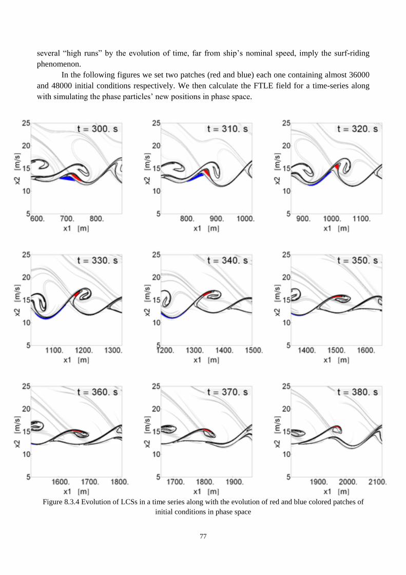
77

several “high runs” by the evolution of time, far from ship’s nominal speed, imply the surf-riding

phenomenon.

In the following figures we set two patches (red and blue) each one containing almost 36000

and 48000 initial conditions respectively. We then calculate the FTLE field for a time-series along

with simulating the phase particles’ new positions in phase space.

Figure 8.3.4 Evolution of LCSs in a time series along with the evolution of red and blue colored patches of

initial conditions in phase space

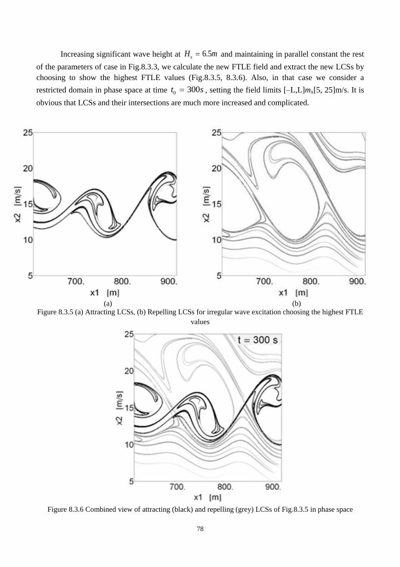
78

Increasing significant wave height at 6.5sH m and maintaining in parallel constant the rest

of the parameters of case in Fig.8.3.3, we calculate the new FTLE field and extract the new LCSs by

choosing to show the highest FTLE values (Fig.8.3.5, 8.3.6). Also, in that case we consider a

restricted domain in phase space at time 0 300t s , setting the field limits [–L,L]mx[5, 25]m/s. It is

obvious that LCSs and their intersections are much more increased and complicated.

(a) (b)

Figure 8.3.5 (a) Attracting LCSs, (b) Repelling LCSs for irregular wave excitation choosing the highest FTLE

values

Figure 8.3.6 Combined view of attracting (black) and repelling (grey) LCSs of Fig.8.3.5 in phase space

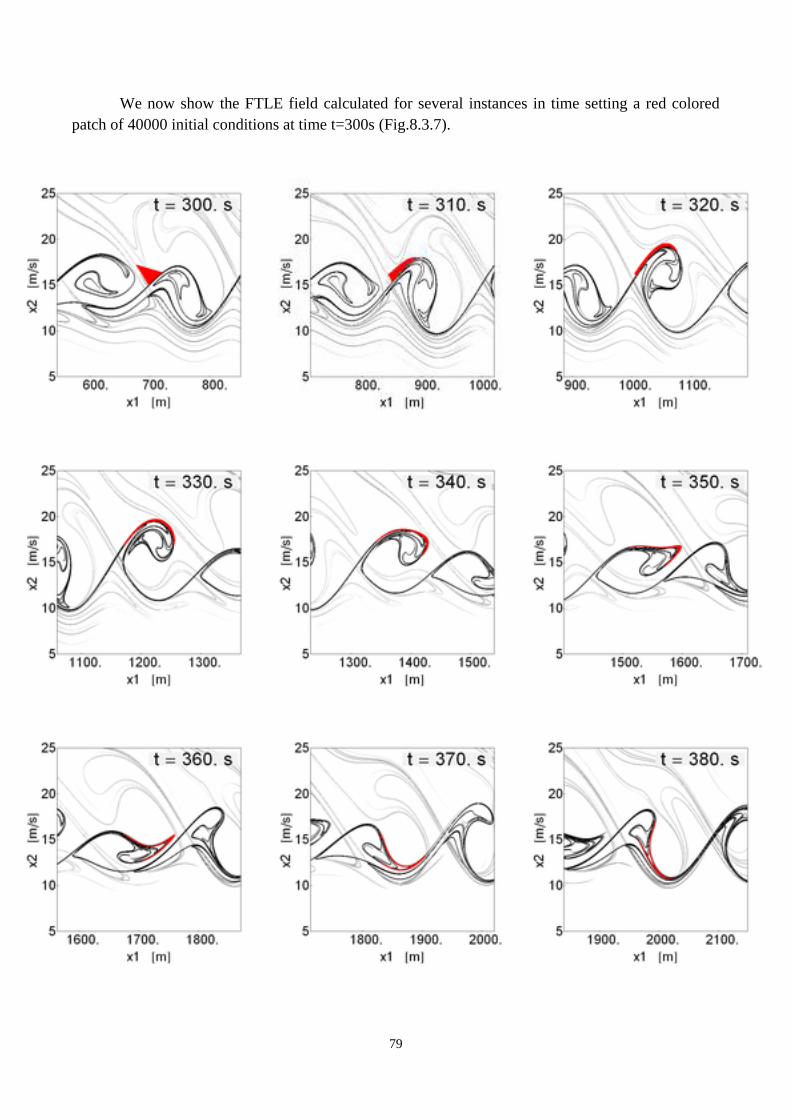
79

We now show the FTLE field calculated for several instances in time setting a red colored

patch of 40000 initial conditions at time t=300s (Fig.8.3.7).

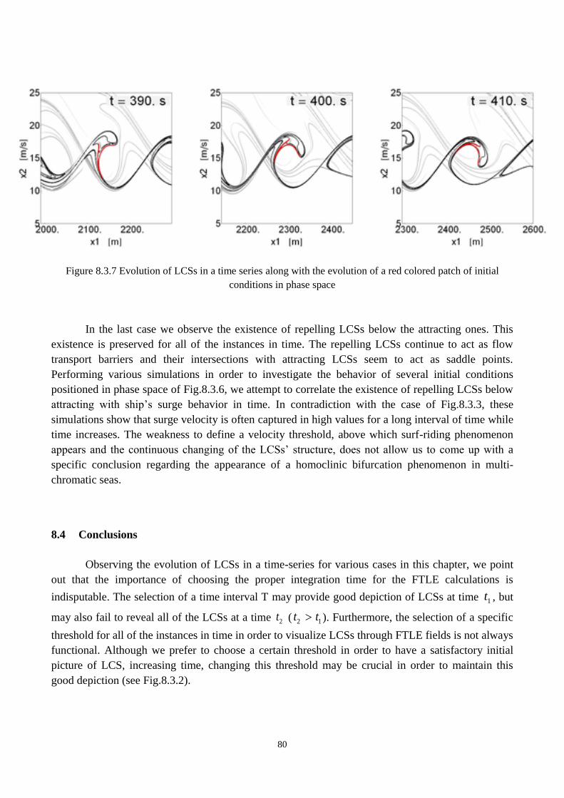
80

Figure 8.3.7 Evolution of LCSs in a time series along with the evolution of a red colored patch of initial

conditions in phase space

In the last case we observe the existence of repelling LCSs below the attracting ones. This

existence is preserved for all of the instances in time. The repelling LCSs continue to act as flow

transport barriers and their intersections with attracting LCSs seem to act as saddle points.

Performing various simulations in order to investigate the behavior of several initial conditions

positioned in phase space of Fig.8.3.6, we attempt to correlate the existence of repelling LCSs below

attracting with ship’s surge behavior in time. In contradiction with the case of Fig.8.3.3, these

simulations show that surge velocity is often captured in high values for a long interval of time while

time increases. The weakness to define a velocity threshold, above which surf-riding phenomenon

appears and the continuous changing of the LCSs’ structure, does not allow us to come up with a

specific conclusion regarding the appearance of a homoclinic bifurcation phenomenon in multi-

chromatic seas.

8.4 Conclusions

Observing the evolution of LCSs in a time-series for various cases in this chapter, we point

out that the importance of choosing the proper integration time for the FTLE calculations is

indisputable. The selection of a time interval T may provide good depiction of LCSs at time 1t , but

may also fail to reveal all of the LCSs at a time 2t ( 2 1t t ). Furthermore, the selection of a specific

threshold for all of the instances in time in order to visualize LCSs through FTLE fields is not always

functional. Although we prefer to choose a certain threshold in order to have a satisfactory initial

picture of LCS, increasing time, changing this threshold may be crucial in order to maintain this

good depiction (see Fig.8.3.2).

81

9 Discussion and Conclusions

In this thesis, an investigation of the ship’s dynamical behavior in surge direction was made. The

need to understand the nonlinear and time-dependent phenomena in bi-chromatic and multi-

chromatic sea environment through the phase flow analysis stimulated us to implement the FTLE

method in order to extract LCSs.

In our 2-Dimensional phase space, LCSs are curves that act as transport barriers of phase

flow. In fact, these curves are material lines where local maximum stretching appears. Repelling

(attracting) LCSs repel (attract) nearby particles in the largest rate. Extended literature has proved

that in most cases these curves are comparable to stable and unstable manifolds of autonomous

dynamical systems that delineate domains of different dynamical behavior (surging and surf-riding)

in phase space which is feasible to calculate for time-dependent dynamical systems. Through the

computation of the largest FTLE fields in phase space for regular wave excitation and also choosing

to show the largest values of these fields, we attempt to approximate the LCSs. Comparing the

revealed LCSs with stable and unstable manifolds, that it is computationally easy to calculate, we

confirm the validity of the method. Implementing the method for bi-chromatic and multi-chromatic

sea we observe the existence of material lines that separate regions in phase space that organize the

transport of flow particles. In most cases, computing these fields for a time-series we are able to

predict the motion of ensembles of phase flow particles and the final destination that they are going

to move on.

Computing the LCEs’ spectrum provides an estimation of the system’s stability. For a region

in phase space, the LCE’s spectrum may show uniform signs implying a specific dynamical

behavior. So, the co-existence of different types of attractors is not obvious. Computation of the

FTLE field enables us to distinguish the curves that separate these regions of different stability.

However, in cases that the system’s behavior is chaotic, the information given from the FTLE spatial

distribution is quite complicated and not clear. For bi-chromatic wave excitation, computation of

LCEs’ spectrum for a case of initial conditions in phase space helps us diagnose the system’s chaotic

behavior.

One of the main weaknesses of the FTLE method is choosing the appropriate integration time

T. Computing the FTLE field and extracting LCSs for a time-series, we observe the evolution of

LCSs and in parallel the appearance of new ones. So, choosing a specific integration time T does not

always assure the revealing of all the LCSs that act as transport barriers in phase space. Furthermore,

in order to obtain clear visualizations of LCSs, the computational cost could be large.

To sum up, although ship’s surge motion in irregular waves is a complex nonlinear

phenomenon not fully understood until today and also hiding dangerous instabilities, the theory of

extracting LCSs seems to be a precious numerical tool for recognizing domains of different

dynamical behavior and the effects of their interaction.

82

83

10 Further Study

This field of research has mostly been developed in recent years and it is still active with application

in various domains of research and especially in fluid flows.

Regarding the ship’s dynamical behavior more methods of extracting LCSs could be applied

so as to compare them and conclude on specific conclusions on the their reliability (see Haller [9]).

Further investigation could be focused especially on extracting LCSs for ship’s surge motion

due to multi-chromatic wave excitation while for the time-dependent flows more development is

needed in order to extract the strongest repelling or attracting structures. Furthermore, regarding

the surf-riding phenomenon, it would be a challenge for researchers to create a quantitative

parameter through the extraction of LCSs that could be used in order to assess the hazard by the

manifestation of the surf-riding phenomenon. Managing to connect the method with probabilistic

methods is the most important issue that researchers should deal with in the near future, taking under

consideration the establishment of the 2nd

generation intact stability criteria.

84

85

11 References

1. Peters, W., Belenky V., Bassler C., Spyrou K., Umeda N., Bulian G., Altmayer B., ‘The

Second Generation of Intact Stability Criteria: An overview of development’, SNAME

Transactions, 2011

2. Grim, O., ‘Das Schiff in von Achtern Auflaufender See’, Jahrbuch der Schiffbautechnischen

Gesellschaft, Vol.45, pp.264-278,1951

3. Kan, M., ‘Surging of Large Amplitude and Surfriding of Ships in Following Seas’, in Naval

Architecture and Ocean Engineering, The Society of Naval Architects of Japan,

Vol.28,Tokyo, 1990

4. Spyrou, K.J., ‘Dynamic Instability in Quartering Seas: The Behavior of a Ship During

Broaching’, Journal of Ship Research, Vol.40, No.1,pp.46-59, 1996

5. Belenky, V.,Spyrou, K.J, Weems, K., Kenneth M., ‘Evaluation of the Probability of Surf-

riding in Irregular Waves with the Time-Split Method’, Proceedings of the 11th

International

Conference on the Stability of Ships and Ocean Vehicles, Athens, Greece, pp.29-37,2012

6. Kontolefas Ioannis and K.J Spyrou, ‘Coherent Phase-space Structures Governing Surge

Dynamics in Astern Seas’,Proceedings,12th International Conference on Stability of Ships

and Ocean Vehicles (STAB2015),pp.1077-1085, Glasgow, 2015

7. Haller, G., Yuan, G., ‘Lagrangian Coherent Structures and Mixing in two-dimensional

turbulence’, Physica D., 147, pp.352-370,2000

8. Shadden, S.C., Lekien, F., Marsden, J.E, ‘Definition and Properties of Lagrangian Coherent

Structures from Finite-Time Lyapunov Exponents in two-Dimensional Aperiodic Flows’,

Physica D 212, 271-304, 2005

9. Haller, G., ‘A variational theory of hyperbolic Lagrangian Structures’, Physica D., 2011

10. Davidson, K.S.M, ‘A Note on the Steering of Ships in Following Seas’,7th

International

Congress of Applied Mechanics, London, England, 1948

11. Grim, O., ‘Surging Motion and Broaching Tendencies in a Severe Irregular Sea’, Deutsche

Hydrographische Zeitschrift, Jahrgang 16, Heft 5.,pp.203-231 ,1963

12. Lyapunov, A.M., ‘Probleme General de la Stabilite du Mouvement’,

Ann.Fac.Sci.Univ.Touluse 9, p.203-475, 1907. Reproduced in Ann. Math. Study, vol.17,

Princeston, 1947

13. Katica (Stevanović) Hedrih, ‘Nonlinear Dynamics and Aleksandr Mikhailovich Lyapunov

(1857-1918)’, Mechanics, Automatic Control and Robotics Vol. 6, No1, pp. 211 – 218, 2007

14. Oseledec, V.I., ‘The Multiplicative Ergodic Theorem. The Lyapunov Characteristic Numbers

of Dynamical Systems’, Trans. Moscow. Math. Soc.19, p.197-231,1968

15. Benettin, G., Galgani, L., Giorgilli, A., Strelcyn, J.M, ‘Lyapunov Characteristic Exponents

for Smooth Dynamixal Systems and Hamiltonian Systems; A Method for Computing all of

them’, Meccanica 15, 1980

16. Wolf, A., Swift, Swinney, J.B., Vastano, J.A., ‘Determining Lyapunov Exponents from a

Time Series’, Physica 16D, 285-317, 1985

17. Sandri, M., ‘Numerical Calculation of Lyapunov Exponents’, The Mathematical Journal,78-

84, 1996

86

18. Boffetta, G., Lacorata, G., Redaelli, G., Vulpiani, A., ‘Detecting barriers to transport: a

review of different techniques’. Physica D 159, 58–70, 2001

19. Peikert R.,Pobitzer A., Sadlo F., Schindler B., ‘A Comparison of Finite-Time and Finite –

Size Lyapunov Exponents’, in Topological Methods in Data Analysis and Visualization III,

Springer, pp.187-200, 2014

20. Haller, G., ‘Distinguished material surfaces and coherent structures in 3D fluid flows’,

Physica D, 2001

21. Haller, G., ‘Lagrangian structures and the rate of a strain in a partition of two-dimensional

turbulence’, Physics of Fluids, Vol.13, No.11, 2001

22. Peacock T. and Haller G., ‘Lagrangian Coherent Structures-The Hidden Skeleton of Fluid

Flows’, www.physicstoday.org,2013

23. Shadden, S.C., ‘Lagrangian Coherent Structures’, Mechanical and Aerospace Engineering,

Illinois Institute of Technology, Chicago,USA,2011

24. Strogatz, S.H., ‘Nonlinear Dynamics and Chaos’, Perseus Books, 2000

25. Klein M. and Baier G., ‘Hierachies of dynamical systems. In a Chaotic Hierachy’,Singapore:

World Scientific,1991

26. Hasselmann K. et al, ‘Measurements of Wind-Wave Growth and Swell Decay during the

Joint North Sea Wave Project (JONSWAP)’, Ergnzungsheft zur Deutschen

Hydrographischen Zeitschrift Reihe, A(8) (Nr. 12), p.95, 1973