BUREAU OF TRANSPORTATION STATISTICS Advisory Council on Transportation Statistics
Bhutan Poverty
assessment 2014
National Statistics Bureau Royal Government of Bhutan The World Bank
Pub
lic D
iscl
osur
e A
utho
rized
Pub
lic D
iscl
osur
e A
utho
rized
Pub
lic D
iscl
osur
e A
utho
rized
Pub
lic D
iscl
osur
e A
utho
rized
Pub
lic D
iscl
osur
e A
utho
rized
Pub
lic D
iscl
osur
e A
utho
rized
Pub
lic D
iscl
osur
e A
utho
rized
Pub
lic D
iscl
osur
e A
utho
rized

Copyright © National Statistics Bureau, 2014 www.nsb.gov.bt
ISBN 979-99936-28-26-2
Design by Loday Natshog Communications ([email protected])

iiiBhutan Poverty Assessment 2014
Acknowledgements iv
Foreword v
Foreword vi
Abbreviations and Acronyms vii
Executive Summary viii
CHAPTER 1: Introduction 01
CHAPTER 2: Evolution of Poverty, Shared Prosperity and Inequality in Bhutan 052.1. Consumption Poverty, Multidimensional Poverty and Happiness 05
2.1.1. Decline in Multidimensional poverty between 2007 and 2012 07
2.1.2. Shared Prosperity 09
2.1.3. Mobility in and out of Poverty between 2007 and 2012 09
2.1.4. Growth in Bhutan has been Pro-Poor 10
2.2. Stable Inequality 12
2.2.1. Uneven Poverty Reduction across Dzongkhags 13
CHAPTER 3: Changing Profiles of the Poor and Bottom 40 Percent of the Population 173.1. Welfare Indicators (Assets and Amenities) 17
3.2. Health and Nutrition 18
3.3. Gender and Poverty 22
3.3.1. Is Poverty in Bhutan Gender-Blind? 22
3.4. Land Ownership and Poverty 23
CHAPTER 4: Enlarging Opportunities for Children 274.1. Inequality of Opportunity in Bhutan 27
4.2. Social Outcomes for Children in Relation to Birth Circumstances 29
4.3. Measuring Inequality of Opportunity 35
4.4. Drivers of Change 42
CHAPTER 5: Key Drivers of Poverty Reduction in Bhutan 455.1. Trading Out of Poverty 47
5.2. Roads Out of Poverty 50
5.3. The Hydro Effect 53
5.4. Who were Better Able to Escape Poverty between 2007 and 2012? 53
5.5. The Main Drivers of Poverty Reduction from People’s Perspective 54
5.6. Better Returns on Individual’s Assets Underpin Faster Reduction in Poverty 55
5.7. Composition versus Structure 56
CHAPTER 6: Poverty Reduction in Bhutan: Sustainability, Vulnerability and Suggested Remediation 61
Annex A: Sources of Variation in Poverty Outcomes in Bhutan 68
Annex B: Poverty Dynamics with Synthetic Panels – Framework and Results 88
Annex C: Qualitative Assessment of Poverty 101
Con
tent
s
iv Bhutan Poverty Assessment 2014
Acknowledgements
This report is the first poverty assessment for Bhutan prepared by the World Bank jointly with the Royal Government of Bhutan through the National Statistics Bureau (NSB). It builds on Bhutan Poverty Analysis 2012, published by the NSB with technical assistance from the World Bank.
The study is led by Srinivasan Thirumalai (Senior Economist, SASEP) with team members drawn from the World Bank, NSB, and outside consultants. The Bank team comprised of Peter Lanjouw and Hai-Anh Dang (DECRG), Namgyel Wangchuk (SASEP), Minh Cong Nguyen (ECSP3), and Smriti Seth (DECWB). From the NSB’s Socio-Economic Analysis and Research Division, Lham Dorji (Dy. Chief Research Officer), Dorji Lethro (Senior Statistical Officer), Sonam Gyeltshen (Research Officer), and Cheku Dorji (Dy. Chief Statistical Officer, Coordination and Information Division) worked closely with the World Bank team. Consultants who contributed to the study are Essama-Nssah, Nar Bahadur Chhetri, Krishna Parajuli and Sanjana Dulal.
We give special thanks to local officials and elected representatives (Gups) who facilitated focus group discussions and shared their views on development issues at the local level. In this regard, we wish to especially thank
Tenzin Thinley (Dzongdag), Lhawang Dorji and Thinley Wangchuk (Gups) in Dagana, Karma Drukpa (Dzongdag), Tashi Rabten (GAO), Rinchen Lungten (Gup) in Zhemgang, Karma Wangdi (Dzongrab), Lepo and Chedup (Gups), Dawa Zangmo (GAO) in Pema Gatshel, Sonam Wangyel (Dzongdag), Karma and Tshering Samdrup (Gups) and Kinley Phuntsho (GAO) in Lhuentse. Focus group participants shared candid views and debated priority issues with endearing keenness.
The team benefited from the comments of peer reviewers Sabina Alkire, Vikram Nehru, Dean Jolliffe, and Sonam Tobgyel at concept stage and also at the final stage. We are grateful for comments by David Newhouse and Genevieve Boyreau for comments on an initial draft. We are thankful to the participants at the final review meeting held in Washington D.C and a consultative group meeting held in Thimphu to discuss the findings of the report.
Overall guidance for the study was provided by Ernesto May, Director (SASEP), Kuenga Tshering, Director General (NSB), Vinaya Swaroop (SASEP), Robert Saum (Country Director) and Genevieve Boyreau (Resident Representative).
vBhutan Poverty Assessment 2014
Foreword
The National Statistics Bureau is pleased to present the Bhutan Poverty Assessment 2014 report prepared in collaboration with the World Bank. This report is a complement to the earlier Poverty Analysis Report (PAR) 2012 which was prepared with the World Bank’s Technical Support. The PAR 2012 provides estimates of consumption poverty, identified the trend and narrates the profile of the poor in terms of demographics and basic needs. Most of the poverty reduction in Bhutan has occurred in the rural areas with little change in urban poverty rates. Inequality has not changed significantly. Poverty reduction in dzongkhags have been found to be uneven.
This report identifies the key drivers of rapid poverty reduction in Bhutan over the recent years, explaining why some dzongkhags are stuck in poverty or reducing poverty is not significant while others prospered, and whether female headed households have a harder time reducing poverty. The exercise draws mainly on data from the two rounds of Bhutan Living Standards Survey (2007 and 2012) supplemented with focus group discussions carried out for the report in select dzongkhags.
The report presents a more detailed analysis of the evolution of poverty, its distributional characteristics including inequality, mobility estimates; changing profiles of the poor and bottom 40 percent of the population; issues in expanding opportunities for children. This report probes the vulnerabilities in spreading prosperity in Bhutan and discusses the steps to be taken for sustained poverty reduction in Bhutan.
One of the factors contributing to poverty reductions is due to the noble Royal Kidu Program where many landless households were able to get land permanently registered in their names. The findings from the participatory assessments listed small land holdings and landlessness as key constraints to achieving economies of scale in agricultural production.
This assessment report also shows that, among others, Bhutan’s poverty reduction has been rapid, broad-based and inclusive; in the long-term, sustainable poverty reduction depends on addressing persistent shocks, engendering private sector led development and defining clear target groups for poverty reduction. The main drivers of prosperity in rural Bhutan appear to be increasing commercialization of agriculture, an expanding rural road network and beneficial spillovers from hydroelectric projects.
I hope that this report becomes a comprehensive source of information towards further reduction of poverty especially in sections and areas where the poverty still remains high.
Finally, I wish to sincerely thank the World Bank for their continued support and would like to acknowledge the efforts of all officials and experts who were involved in this important exercise.
(Kuenga Tshering)Director General
vi Bhutan Poverty Assessment 2014
Foreword
This report presents the first Poverty Assessment carried out in Bhutan by the World Bank in close collaboration with the National Statistics Bureau, Bhutan.
Bhutan well known as a pioneer of the Gross National Happiness concept has a noteworthy record in reducing poverty as well. Poverty reduction in Bhutan, as the report finds, has been rapid, broad-based and inclusive. Prosperity has been shared well in Bhutan with the bottom 40 percent enjoying faster growth than the rest. There are potentially useful lessons for other countries aspiring for poverty reduction with shared prosperity.
Poverty reduction in Bhutan is well-founded in long-term economic development efforts of commercialization of agriculture, expanding rural road networks and beneficial spillovers from hydroelectric projects. A good governance infrastructure underpins the successes on poverty front. The pace of poverty reduction appears sustainable if the emerging risks and vulnerabilities are managed carefully.
Sustaining the examplary record of Bhutan's poverty reduction in the long-term would require mitigating risks from persistent shocks facing the agricultural sector, increasing reliance on private sector led development and building formal social protection for clearly identified population groups most vulnerable to poverty.
The findings of the report have directly influenced our engagement in Bhutan as reflected
in our "Country Partnership Strategy 2014-2019". The identified drivers of poverty reduction and recommendations have translated into : (i) a focus on agriculture commercialization and marketization, and more broadly the sustainable contribution of green assets to socio-economic development, (ii) supporting a social protection strategy, with targeted safety nets build household's resilience, (iii) a continued focus on the private sector development to create jobs which improve living standards and are also a critical element of social cohesion, (iv) a renewed attention to transport and trade infrastructure, recognizing its critical role in reducing poverty; (v) improving fiscal and spending efficiency to enable the Royal Government to continue improving the delivery of public services for the benefit of all.
We - at the World Bank - are committed to support shared prosperity and the fight against poverty throughout the world, and in Bhutan in particular, where we look forward to building on a strong partnership with the Royal Government and all stakeholders.
Genevieve Boyreau Resident Representative World Bank, Bhutan

viiBhutan Poverty Assessment 2014
GOVERNMENT FISCAL YEARJuly 1 – June 30
CURRENCY EQUIVALENTSCurrency Unit = Bhutanese Ngultrum (Nu)
US$1 = Nu 61.8 (March 25, 2014)
Abbreviations and Acronyms
BIMSTEC Bengal Initiative for Multisectoral Technical and Economic Cooperation
BLSS Bhutan Living Standards SurveyCBS Centre for Bhutan StudiesCPIA Country Policy and Institutional
AssessmentDDS Dietary Diversity ScoreFANTA Food and Nutrition Technical
AssistanceFAO Food and Agricultural OrganizationFGT Foster-Greer-ThorbeckeFYP Five Year PlanGAO Gewog Administrative OfficerGDP Gross Domestic ProductGIC Growth Incidence CurveGNH Gross National HappinessHDDS Household Dietary Diversity ScoreHIV Human Immunodeficiency VirusHOI Human Opportunity Index
MDG Millennium Development GoalMIC Middle Income CountryMoAF Ministry of Agriculture and ForestMPI Multidimensional Poverty IndexNPL National Poverty LineNSB National Statistics BureauOGTP One Gewog Three ProductsPAR Poverty Assessment ReportRGoB Royal Government of BhutanRNR Renewable Natural ResourcesSAARC South Asian Association for Regional
CooperationSAFTA South Asia Free Trade AgreementSAR South Asia RegionSL Standard of LivingTIP Three “I”s (incidence, intensity and
inequality) of Poverty
viii Bhutan Poverty Assessment 2014
Executive Summary
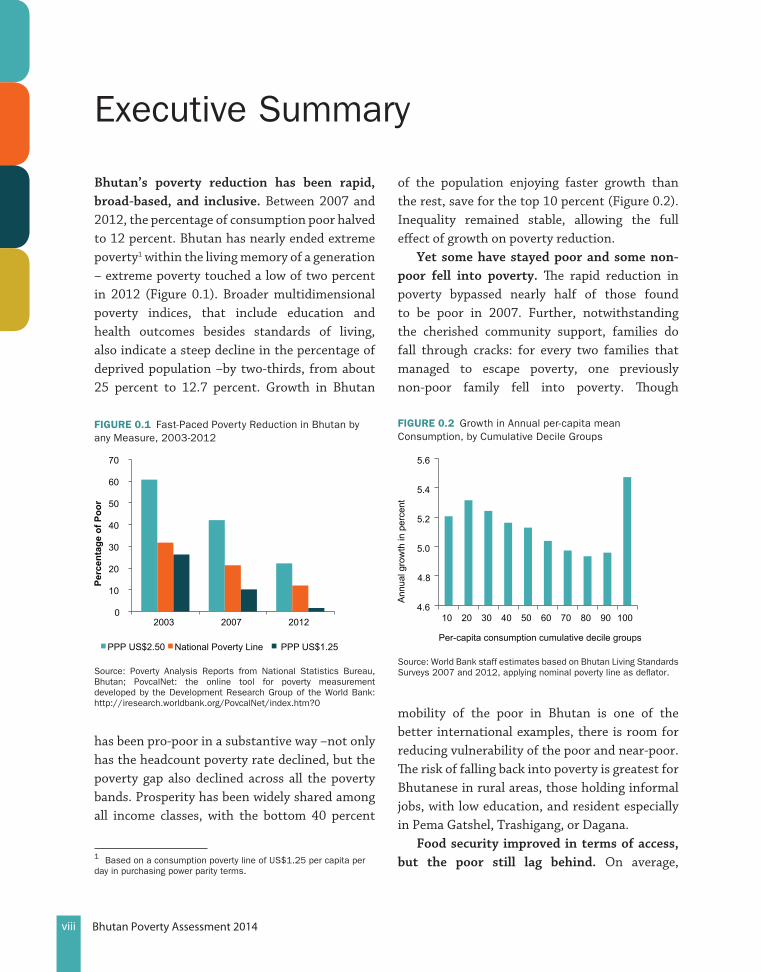
Bhutan’s poverty reduction has been rapid, broad-based, and inclusive. Between 2007 and 2012, the percentage of consumption poor halved to 12 percent. Bhutan has nearly ended extreme poverty1 within the living memory of a generation – extreme poverty touched a low of two percent in 2012 (Figure 0.1). Broader multidimensional poverty indices, that include education and health outcomes besides standards of living, also indicate a steep decline in the percentage of deprived population –by two-thirds, from about 25 percent to 12.7 percent. Growth in Bhutan
has been pro-poor in a substantive way –not only has the headcount poverty rate declined, but the poverty gap also declined across all the poverty bands. Prosperity has been widely shared among all income classes, with the bottom 40 percent
1 Based on a consumption poverty line of US$1.25 per capita per day in purchasing power parity terms.
of the population enjoying faster growth than the rest, save for the top 10 percent (Figure 0.2). Inequality remained stable, allowing the full effect of growth on poverty reduction.
Yet some have stayed poor and some non-poor fell into poverty. The rapid reduction in poverty bypassed nearly half of those found to be poor in 2007. Further, notwithstanding the cherished community support, families do fall through cracks: for every two families that managed to escape poverty, one previously non-poor family fell into poverty. Though
mobility of the poor in Bhutan is one of the better international examples, there is room for reducing vulnerability of the poor and near-poor. The risk of falling back into poverty is greatest for Bhutanese in rural areas, those holding informal jobs, with low education, and resident especially in Pema Gatshel, Trashigang, or Dagana.
Food security improved in terms of access, but the poor still lag behind. On average,
FIguRE 0.1 Fast-Paced Poverty Reduction in Bhutan by any Measure, 2003-2012
0
10
20
30
40
50
60
70
2003 2007 2012
Perc
enta
ge o
f Poo
r
PPP US$2.50 National Poverty Line PPP US$1.25
Source: Poverty Analysis Reports from National Statistics Bureau, Bhutan; PovcalNet: the online tool for poverty measurement developed by the Development Research Group of the World Bank: http://iresearch.worldbank.org/PovcalNet/index.htm?0
FIguRE 0.2 Growth in Annual per-capita mean Consumption, by Cumulative Decile Groups
4.6
4.8
5.0
5.2
5.4
5.6
10 20 30 40 50 60 70 80 90 100
Ann
ual g
row
th in
per
cent
Per-capita consumption cumulative decile groups
Source: World Bank staff estimates based on Bhutan Living Standards Surveys 2007 and 2012, applying nominal poverty line as deflator.
ixBhutan Poverty Assessment 2014
Bhutanese increased dietary diversity by consuming from 10 food groups (out of 12) in 2012, from just seven groups in 2007. Protein sources, especially, have increased to include meat, fish, and pulses. However, the poor lag behind in access to diversified food groups, particularly protein sources. In addition, inadequate food is reported by 10 percent of poor households – more than double the non-poor’s four percent.
Female-headed households are not on par with male-headed households in enjoying fruits of growth. Thirty percent of Bhutanese households are headed by females. While the poverty incidence (consumption or multidimensional poverty rate) is found to be equal for both male- and female-headed households, some female groups (notably married and divorced) have a greater incidence of poverty than the corresponding male groups; the bottom 40 percent of female-headed households enjoyed a smaller rise in consumption compared to that of their male-headed counterparts. The persistence of the livelihood handicap for female-headed households, despite matrilineal inheritance and a non-discriminatory labour market, suggests that disproportionate household burdens may be diminishing opportunities for women.
Opportunities for children are equalizing regardless of birth circumstances but inequities in completion of secondary education persist. Bhutanese children have better and improving opportunities in education and infrastructure services than those of other South Asian countries, and these opportunities are becoming more equal across income classes. The public policy of extending coverage for all and targeting interventions with electricity and gas provision have narrowed inequalities among children. Nevertheless, it is important to note that inequity in completion of secondary education remains an issue–the inequality-adjusted completion rate was only 32 percent in 2012, with an adjusted
attendance of 84 percent. Higher completion rates alone would help to build comparative advantage for Bhutanese youth in skilled labour.
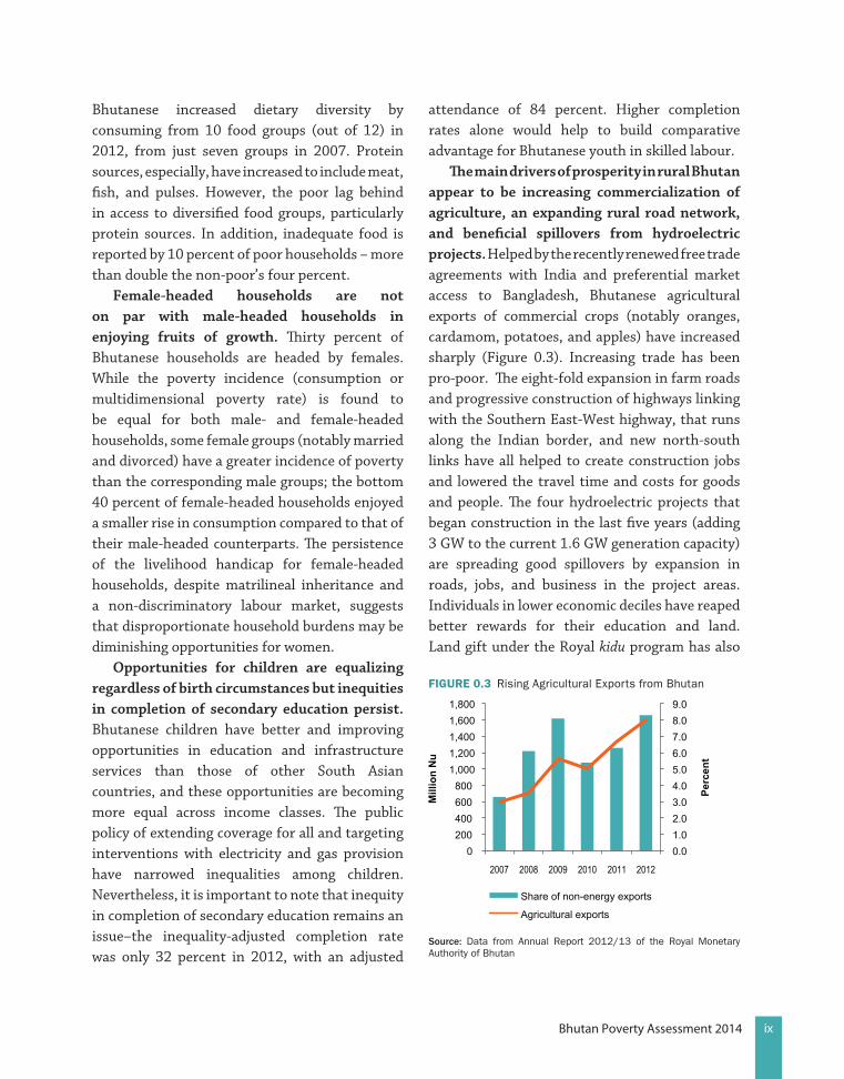
The main drivers of prosperity in rural Bhutan appear to be increasing commercialization of agriculture, an expanding rural road network, and beneficial spillovers from hydroelectric projects. Helped by the recently renewed free trade agreements with India and preferential market access to Bangladesh, Bhutanese agricultural exports of commercial crops (notably oranges, cardamom, potatoes, and apples) have increased sharply (Figure 0.3). Increasing trade has been pro-poor. The eight-fold expansion in farm roads and progressive construction of highways linking with the Southern East-West highway, that runs along the Indian border, and new north-south links have all helped to create construction jobs and lowered the travel time and costs for goods and people. The four hydroelectric projects that began construction in the last five years (adding 3 GW to the current 1.6 GW generation capacity) are spreading good spillovers by expansion in roads, jobs, and business in the project areas. Individuals in lower economic deciles have reaped better rewards for their education and land. Land gift under the Royal kidu program has also
FIguRE 0.3 Rising Agricultural Exports from Bhutan
0.0 1.0 2.0 3.0 4.0 5.0 6.0 7.0 8.0 9.0
0 200 400 600 800
1,000 1,200 1,400 1,600 1,800
2007 2008 2009 2010 2011 2012
Perc
ent
Mill
ion
Nu
Share of non-energy exports
Agricultural exports
source: Data from Annual Report 2012/13 of the Royal Monetary Authority of Bhutan
x Bhutan Poverty Assessment 2014
helped the previously landless to escape poverty. Education appears to be the most important route by far to escape poverty.
The current pace of poverty reduction appears sustainable in the medium term. Trade intensification with neighbors is set to continue, road infrastructure is posed for more expansion, and more hydroelectric project construction is planned to continue to 2020; the current free trade agreement with India, due for renewal in 2016, is most likely to be renewed. The bilateral agreement with Bangladesh, that has benefited Bhutan by preferential duty-free access to 74 mostly agricultural exports, is also due for renewal, in 2018. In addition bilateral agreements with Thailand and Nepal are also on the anvil. Bhutan is a net exporter of fruits and cardamom in the north-east region of the Indian sub-continent and should be able to sustain fruit exports to Bangladesh even with future preference erosion under the South Asian Free Trade Agreement (SAFTA). Growth dynamism in India and Bangladesh should be able to further accommodate expansion of differentiated agricultural exports from Bhutan which are well known for superior quality. Completion of the Southern East-West highway in Bhutan and expansion of the rural roads network would help to draw out the comparative advantages of Bhutanese agriculture. The hydroelectric projects now under construction are expected to continue to 2016/17, and more projects are planned that would continue to boost rural incomes indirectly. Despite rapid urbanization – one percent of rural population moving every year to urban areas – urban poverty has remained under two percent, indicating that migration is not biased particularly to the poorer sections of the society.
For sustained poverty reduction, risks and vulnerabilities need to be managed carefully. With limited land, increasing fragmentation of land holdings, and rural-to-urban migration of
working age adults, labour-intensive horticulture will become increasingly difficult. Contract farming by large-scale land owners may be a way to sustain exports but benefits to poorer farmers might diminish. The current problems faced by farmers such as the incurable “greening disease” of oranges, diseases of the cardamom plants and regular raids into farms by elephants (in low land), monkeys, and wild boars have persisted. The plan for introducing disease-resistant cultivars is not proceeding swiftly. It takes years to bring horticultural crops to harvest and equally long to shift to other profitable forms of production. As a consequence of increasing commercial crop production, Bhutan dependence on food imports has been rising over the years, making it more vulnerable to food price shocks. A 12 percent increase in food prices – the average annual increase in recent years - for example, can increase the percentage of poor in the short-term by about two percent points. With all petroleum products imported, Bhutan’s poor also face risk from fuel price shocks. A sharp rise in the consumer prices of LPG and kerosene of the order that occurred in July 2013 (quickly reversed, however) had the potential to push 0.5 percent of population into poverty. Bhutan’s social protection is mainly through the Royal Kidu welfare program. Risks of downward mobility are greater than average for rural residents, male-headed households, people in informal jobs (the casually and self-employed), and those with low education and particularly high for those living in select dzongkhags such as Pema Gatshel, Dagana, Samtse, Trashigang, and Tsirang).
Formal social protection programs may be necessary to help individuals cope with adverse economic and financial shocks. At present, individuals cope with shocks mostly by drawing on own savings if they are non-poor, or by borrowing from friends, suppliers, and money-lenders if they are poor. Because of the
xiBhutan Poverty Assessment 2014
inadequacy and inelasticity of these sources for the poor and vulnerable segments of the population, we suggest the introduction of formal social protection mechanisms and possibly well-targeted micro-credit programs.
In the long-term, sustainable poverty reduction depends on addressing persistent shocks, engendering private sector led development and defining clear target groups for poverty reduction. The feasibility of crop insurance for farmers may be examined to protect the harvests from perils of diseases. Other perils, such as those associated with wild-life predation, have also persisted and evaded viable solutions. What poor people want to better their living standards in the long term can be summed up as access to roads, electricity, public transportation, irrigation, land and higher education. Sustained poverty reduction depends on job opportunities and wage earnings of the poor. The development paradigm for a renewable resource rich country like Bhutan would call for engendering private sector led growth actively enabled by the public sector. Successful agribusiness – an emerging sector in Bhutan - will require development of value chain system (from farm to market) that will identify and remove the bottlenecks that farmers encounter including constraints related to finance and availability of crop insurance. The government could engender private investment in
hydropower sector by Private Public Partnerships and subcontracting in order to create jobs. The Royal Government of Bhutan seems to favor complementary use of consumption and multidimensional poverty. But the overlap of the two approaches identifying the poor is small. Therefore defining a clear target group for poverty reduction is important. Also, with success in reducing extreme consumption poverty rapidly, the goal could be now shift to shared prosperity defined for example as the welfare of the bottom 40 percent of the population.
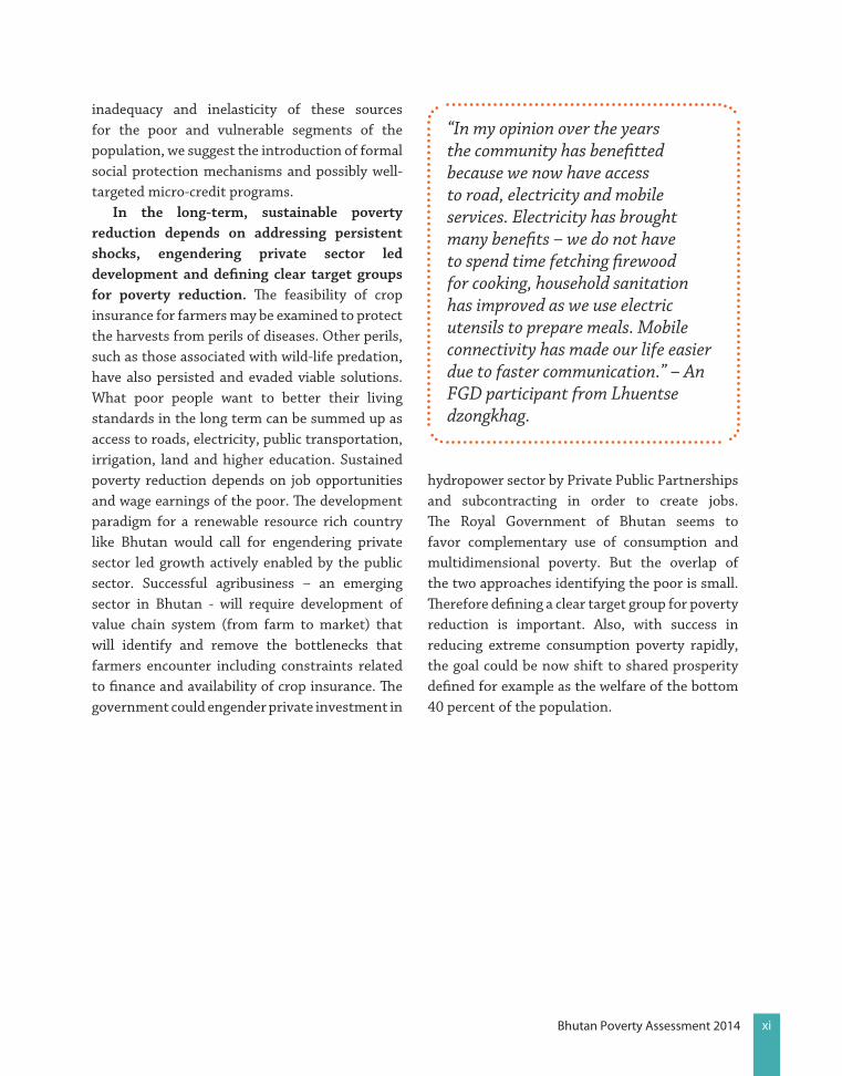
“In my opinion over the years the community has benefitted because we now have access to road, electricity and mobile services. Electricity has brought many benefits – we do not have to spend time fetching firewood for cooking, household sanitation has improved as we use electric utensils to prepare meals. Mobile connectivity has made our life easier due to faster communication.” – An FGD participant from Lhuentse dzongkhag.

01Bhutan Poverty Assessment 2014
Introduction
Bhutan’s location provides opportunities and challenges. Land-locked in the eastern Himalayas, Bhutan is bordered by two Asian giants, China and India. Its population density, at 19 persons per sq. km, is the lowest in South Asia. Elevation ranges from 200 meters in the southern foothills to some peaks in the north that are around 7,000 meters above sea level. Bhutan’s picturesque topography consists of tall mountains, thick forests and tumultuous rivers. In keeping with its philosophy of sustainable development, Bhutan’s constitution requires that 60 percent of its land area be covered by forests (around 72 percent of the land was under forest cover in 2011). Renewable fresh water availability, at 106,933 cubic meters per capita, is the third-highest in the world. Challenges include difficult terrain (tall mountains with sheer drops) that makes connecting remote areas difficult and expensive, and a small and dispersed population that limits economies of scale. Moreover, Bhutan is located on the Indian and Eurasian tectonic plates, whose movements and collisions cause frequent earthquakes in the area. It also experiences other disasters such as landslides, forest fires, and glacial lake outburst floods.
Bhutan has enjoyed continued political stability, strong institutions and good
governance. The country transitioned from an absolute monarchy to a constitutional monarchy with a multi-party democracy in 2008. The second democratic process has evolved, with multiple political parties participating in the July 2013 parliamentary elections for the lower house. Its Country Policy and Institutional Assessment (CPIA) rates fairly well and so do international measures of governance and corruption. With regard to corruption perception, Bhutan ranks 31st among 177 countries and scores better than Israel, Spain, and Poland. Domestic perception of corruption is on the decline, as reflected in the increase of the Bhutan Comprehensive integrity score in recent years.
Bhutan is on its way towards Middle Income Country (MIC) status, has a unique poverty reduction record in international context. Its GDP per capita is already US$ 2,584 in 2012 and it is poised for eight percent growth over the coming five years. It has done well on poverty alleviation and providing service to citizens.
Bhutan has made stellar progress in meeting MDGs and extending gains beyond GDP growth. Of the eight MDGs, seven are actionable to national policies. Among these seven, Bhutan has already achieved or over-achieved four goals in halving extreme poverty, reaching gender
1Chapter

02 Bhutan Poverty Assessment 2014
parity in education, ensuring environmental sustainability, and reducing by three-fourths maternal mortality. Notably, in many of these, Bhutan’s initial conditions were worse than its neighbors’ but had surpassed the neighbors’ by 2011. For instance, maternal mortality in 1990 was at 1,000 per 100,000 – much worse than India’s 600, but by 2011 it had fallen to 180 while India’s was still around 200. In the remaining three goals –universal primary enrollment, halting and reversing the spread of communicable diseases, and reducing by one-third infant and under-5 mortality – Bhutan is on track. Some areas still requiring attention under the MDGs are gender parity in tertiary education, detection of HIV cases, and youth unemployment. Significant progress has been made towards gender equality: in education, female enrollment in primary schools stood at 88 percent in 2008 compared to one girl enrolled for every 50 boys in 1970; maternal mortality has dropped dramatically (as noted above, to 180 from 1,000 in 1990), and women are almost at parity in the labour force.
The Royal Government of Bhutan (RGoB) has made the pursuit of national happiness the overarching goal of its development strategy. In that context, it is committed to improving the quality of life for the citizens through inclusive and sustainable economic growth, the conservation of the natural environment, the preservation of the country’s cultural heritage and good governance. These focal areas constitute the four pillars spanning the concept of Gross National Happiness (GNH), and are being implemented through a series of five year plans. The vision underlying this strategic framework has been enshrined in the 2008 Constitution,2 adopted at the beginning of the 10th Five Year Plan (2008-2013).
2 This Constitution marks a transition in the system of government from absolute monarchy to a parliamentary democracy.
Recognizing the fact that political democracy and economic empowerment do reinforce each other, the government has made poverty reduction the central theme and main objective of the 10th Five Year Plan. It intends to pursue this objective through industrial development, national spatial planning, and integrated rural-urban development, a strategic expansion of infrastructure, human capital development, and enhancing the enabling environment. The formulation of the 10th Five Year Plan builds on the strong achievements of the Ninth Plan (2002-2007) which sought to improve the quality of life and income, with a special focus on the poor, by promoting good governance and private sector-driven economic growth in addition to preserving cultural heritage and the natural environment.
The purpose of this report is to provide an account of the poverty outcomes observed under the 10th Five Year Plan. This account is based on data from the 2007 and 2012 rounds of the Bhutan Living Standards Survey (BLSS). Other quantitative data came from Labour Force Surveys and Renewable Natural Resource (RNR) statistics. This is supplemented by qualitative report from a series of focus group discussions (FGD) held for the study in four dzongkhags of Bhutan. Given the period of this plan, the 2007 data provide a valid baseline for an assessment of the poverty outcomes of this plan. Similarly, the 2012 data are considered end-line observations reflecting the outcome of the implementation of the 10th Five Year Plan since the plan ends in 2013.
This report builds on Bhutan Poverty Analysis, 2012–earlier collaborative work between the NSB and the World Bank. While the previous report presented new estimates of consumption-based poverty and characteristics of the poor in 2012, the current report offers a more detailed analysis of the evolution of poverty, its distributional characteristics including inequality, mobility
03Bhutan Poverty Assessment 2014
estimates (Chapter 2), changing profiles of the poor and bottom 40 percent of the population (Chapter 3), issues in expanding opportunities for children – Human Opportunity Indices (Chapter 4), identifies key drivers of poverty reduction in Bhutan (Chapter 5) and examines what are the vulnerabilities and steps to be taken for sustained poverty reduction in Bhutan (Chapter 6).
05Bhutan Poverty Assessment 2014
Evolution of Poverty, Shared Prosperity and Inequality in Bhutan
2.1. Consumption Poverty, multidimen-sional Poverty and happiness
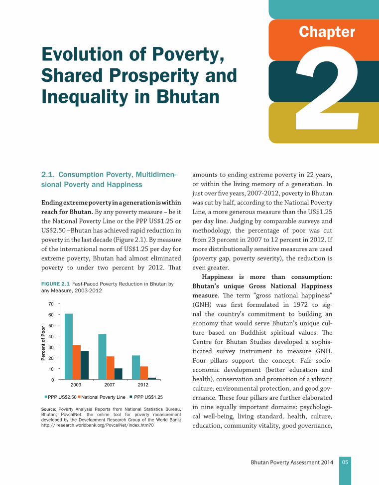
Ending extreme poverty in a generation is within reach for Bhutan. By any poverty measure – be it the National Poverty Line or the PPP US$1.25 or US$2.50 –Bhutan has achieved rapid reduction in poverty in the last decade (Figure 2.1). By measure of the international norm of US$1.25 per day for extreme poverty, Bhutan had almost eliminated poverty to under two percent by 2012. That
amounts to ending extreme poverty in 22 years, or within the living memory of a generation. In just over five years, 2007-2012, poverty in Bhutan was cut by half, according to the National Poverty Line, a more generous measure than the US$1.25 per day line. Judging by comparable surveys and methodology, the percentage of poor was cut from 23 percent in 2007 to 12 percent in 2012. If more distributionally sensitive measures are used (poverty gap, poverty severity), the reduction is even greater.
Happiness is more than consumption: Bhutan’s unique Gross National Happiness measure. The term “gross national happiness” (GNH) was first formulated in 1972 to sig-nal the country’s commitment to building an economy that would serve Bhutan’s unique cul-ture based on Buddhist spiritual values. The Centre for Bhutan Studies developed a sophis-ticated survey instrument to measure GNH.
Four pillars support the concept: Fair socio-economic development (better education and health), conservation and promotion of a vibrant culture, environmental protection, and good gov-ernance. These four pillars are further elaborated in nine equally important domains: psychologi-cal well-being, living standard, health, culture, education, community vitality, good governance,
2Chapter
FIguRE 2.1 Fast-Paced Poverty Reduction in Bhutan by any Measure, 2003-2012
0
10
20
30
40
50
60
70
2003 2007 2012
Perc
ent o
f Poo
r
PPP US$2.50 National Poverty Line PPP US$1.25
source: Poverty Analysis Reports from National Statistics Bureau, Bhutan; PovcalNet: the online tool for poverty measurement developed by the Development Research Group of the World Bank: http://iresearch.worldbank.org/PovcalNet/index.htm?0

06 Bhutan Poverty Assessment 2014
balanced time use, and ecological integration. In accordance with these nine domains, Bhutan has developed 33 clusters and 124 variables that are used to define and analyze the happiness of the Bhutanese people. The GNH concept serves as a unifying vision for Bhutan’s five year planning process and all the derived planning documents that guide the economic and development plans of the country. Proposed policies in Bhutan must pass a GNH review based on a GNH impact as-sessment.
Bhutan has made stellar progress in meeting the MDGs and extending gains beyond GDP growth. Of the eight MDGs, seven are actionable to national policies. Of these seven, Bhutan has already achieved or over-achieved four goals: halving extreme poverty, reaching gender parity in education, ensuring environmental sustainability, and reducing maternal mortality by three-fourths. Notably, in many of these factors Bhutan’s initial conditions were worse
than its neighbors, but it had surpassed those neighbors by 2011. For instance, maternal mortality in 1990 was, at 1,000 per 100,000, much worse than India’s 600, but by 2011 it fallen to 180 while India’s was still around 200. For the remaining three goals –universal primary enrollment, halting and reversing the spread of communicable diseases, and reducing by one-third infant and under-5 mortality – Bhutan is on track. Some areas requiring attention under the MDGs are gender parity in tertiary education, detection of HIV cases, and youth unemployment.
Bhutan’s poverty reduction record is unique. Using the internationally comparable US$1.25 per day poverty line, Bhutan stands out for the pace of its poverty reduction compared to other South Asian countries and the select cohort of countries with similar initial poverty levels in 1990. Starting from about the same level as that of the South Asia region in
FIguRE 2.2 Bhutan Outpaces South Asia Region in Poverty Reduction
FIguRE 2.3 Bhutan Poverty Reduction Leads Countries with Similar 1990 Poverty Levels
0.0
10.0
20.0
30.0
40.0
50.0
60.0
1990 1999 2010
Developing World South Asia Bhutan
0
10
20
30
40
50
60
70
1990 1999 2010
Lesotho India* Ethiopia
LaoPDR Ghana Sudan
Indonesia* Cambodia Pakistan
China* Bhutan
source: PovcalNet: the online tool for poverty measurement developed by the Development Research Group of the World Bank: http://iresearch.worldbank.org/PovcalNet/index.htm?0Note: In Figure 2.3, asterisks indicate estimates aggregated from rural and urban data.
07Bhutan Poverty Assessment 2014
1990,and with more than half of its population in poverty, Bhutan had managed to reduce the percentage of poor to a mere four percent by 2010,while the whole of South Asia’s poverty level had fallen to 30 percent (Figure 2.2). Among those countries in the developing world that had poverty in the 50-60 percent range in 1990, Bhutan’s poverty reduction has been the steepest (Figure 2.3).
2.1.1. Decline in multidimensional poverty between 2007 and 2012
The 10th Five-Year Plan adopted by the Bhutanese government prioritizes poverty reduction in a multidimensional way. Given the limitations of consumption poverty measures in capturing overall deprivation, the government also estimates a more holistic measure called the multidimensional poverty index (MPI). The MPI, which is based on the concept of capability deprivation, uses the Alkire Foster methodology with three equally weighted dimensions –health, education, and standard of living – each of which is further split into two, two, and nine sub-indicators, respectively. A household that is deprived 4/13of the weighted indicators is MPI-poor.
In 2012, 12.7 percent of the country’s population was MPI-poor –not different from the 12 percent headcount ratio for consumption poverty but only 3.2 percent of the population was both consumption and MPI-poor at the same time. This huge mismatch between the two measures illustrates the importance of two measures. However, there was greater overlap in the standard of living (SL) one-seventh of the weight of this dimension is assigned to each of six indicators: electricity, sanitation, water, housing material, cooking fuel and road access, and the remaining one-seventh of the weight is equally distributed among assets, land ownership and
livestock ownership). None of the households were observed to be deprived in all SL indicators, but nearly 70 percent were deprived in at least one, and more than 32 percent were deprived in at least half of all the indicators. Fifty percent of all the consumption-poor were observed to be deprived in at least half of the SL indicators. The highest headcount ratio (36 percent) was observed in the use of solid cooking fuel, followed by no access to improved sanitation facilities (29 percent). Over 10 percent of the population was MPI-poor and used dung, wood, or charcoal for cooking.
Education deprivation was the highest in all three dimensions, with 2.5 percent of the population deprived in both forms of the education indicators (schooling of household members and child attendance), and 27 percent deprived in at least one. Further, 7 percent of the consumption-poor were deprived in both education indicators, while 37 percent was deprived in at least one. Among the income-poor households, nearly 30 percent had no adult with at least five years of education, and 15 percent had school-aged children not attending school.
By comparison, less than one percent of the total population was deprived in both health indicators (food security and child mortality) and 15 percent was deprived in at least one. These deprivations were deepest among the income-poor, where 23 percent of the population
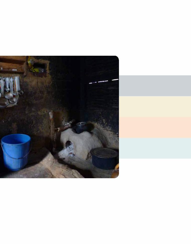
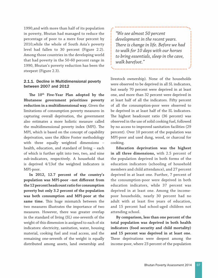
“We see almost 50 percent development in the recent years. There is change in life. Before we had to walk for 10 days with our horses to bring essentials, sleep in the cave, walk barefoot.”
08 Bhutan Poverty Assessment 2014
was deprived in at least one indicator. Further, a higher incidence of child mortality was observed among income-poor households (at 15% of the population) compared to food shortage (9%). While none of the consumption-poor households were deprived in all health and education indicators, nearly 8 percent of them (i.e., 0.9% of the total population) were deprived in at least one health and one education indicator.
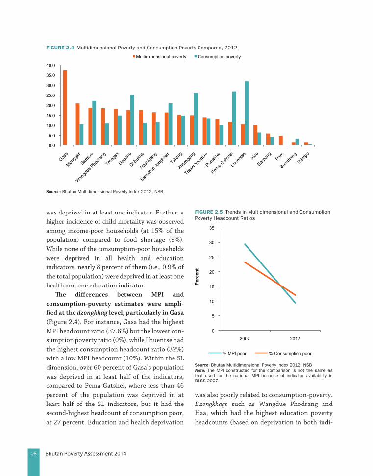
The differences between MPI and consumption-poverty estimates were ampli-fied at the dzongkhag level, particularly in Gasa (Figure 2.4). For instance, Gasa had the highest MPI headcount ratio (37.6%) but the lowest con-sumption poverty ratio (0%), while Lhuentse had the highest consumption headcount ratio (32%) with a low MPI headcount (10%). Within the SL dimension, over 60 percent of Gasa’s population was deprived in at least half of the indicators, compared to Pema Gatshel, where less than 46 percent of the population was deprived in at least half of the SL indicators, but it had the second-highest headcount of consumption poor, at 27 percent. Education and health deprivation
was also poorly related to consumption-poverty. Dzongkhags such as Wangdue Phodrang and Haa, which had the highest education poverty headcounts (based on deprivation in both indi-
FIguRE 2.4 Multidimensional Poverty and Consumption Poverty Compared, 2012
0.0
5.0
10.0
15.0
20.0
25.0
30.0
35.0
40.0
Gasa
Mongg
ar
Samtse
Wangd
ue P
hodra
ng
Trongs
a
Dagan
a
Chhuk
ha
Trashig
ang
Samdru
p Jon
gkha
r
Tsiran
g
Zhemga
ng
Trashi
Yang
tse
Punak
ha
Pema G
atshe
l
Lhue
ntse
Haa
Sarpan
g Paro
Bumtha
ng
Thimpu
Multidimensional poverty Consumption poverty
source: Bhutan Multidimensional Poverty Index 2012, NSB
FIguRE 2.5 Trends in Multidimensional and Consumption Poverty Headcount Ratios
0
5
10
15
20
25
30
35
2007 2012
Perc
ent
% MPI poor % Consumption poor
source: Bhutan Multidimensional Poverty Index 2012, NSBNote: The MPI constructed for the comparison is not the same as that used for the national MPI because of indicator availability in BLSS 2007.

09Bhutan Poverty Assessment 2014
cators), were also among the ten richest in terms of consumption poverty. Similarly, Zhemgang and Pema Gatshel had the lowest health dep-rivation headcounts, but featured among the highest income-poverty headcounts. Further, in Haa and Trashi Yangtse, there were signifi-cant differences in their relative performance on education and health deprivations, highlighting greater inconsistencies across different meas-ures of deprivation.
Time-trend mapping of multidimensional poverty conforms with the decline in consumption poverty. Using comparable sets of indicators, the trend decline in MPI and the headcount of MPI-poor show similar reduction to that of the consumption poverty headcount using the same cutoff value as national MPI – deprivation in one-third of the indicators, although the decline in the MPI-poor headcount ratio is steeper (Figure 2.5).
2.1.2. shared Prosperity
Bhutan’s poorer half enjoyed greater prosperity than the rest, save for the richest decile. In the most recent five-year period, 2007-12, Bhutan as a whole enjoyed an annual per-capita consumption growth of about 5.5 percent in real terms. The bottom 40 percent – the definition used by the World Bank for measuring shared prosperity – of Bhutanese raised their consumption by five percent per year. Aside from the richest decile, therefore, growth has favored the lower classes in Bhutan (Figure 2.6).
2.1.3. mobility in and out of Poverty be-tween 2007 and 2012
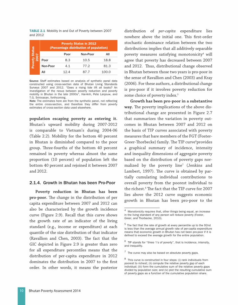
For every two families that escaped poverty, one fell into poverty. Two-thirds of the poor in 2012 were also poor in 2007.The usual poverty estimates based on cross-section data provide a snap-shot and do not inform how many of
the poor were chronically poor and how many moved in and out of poverty. Bhutan does not have panel data – same households surveyed over time. But a synthetic panel can be put together by looking at households with age of head of households restricted to between 25 and 55 for 2007 and increased by 5 years for 2012 for analysis of mobility of households over time3. Using synthetic panel approach, it is found that of the 12.4 percent poor in 2012 and 8.4 percent - two-thirds of all poor were poor also in 2007 (Table 2.1). While 10.5 percent of the population exited poverty between the two periods, 4 percent of the population dropped into poverty from non-poor status.
Mobility in Bhutan compares well with other countries, with twice as many of the
3 Hai-Anh Dang and Peter Lanjouw. 2013. “Measuring Poverty Dynamics with Synthetic Panels Based on Cross-Sections”, World Bank Policy Research Paper number 6504, June 2013. Estimation of point estimates using synthetic panel is a new approach, earlier research by the authors used bound-estimates.
FIguRE 2.6 Growth in Annual per-capita mean Consumption, by Cumulative Decile Groups
4.6
4.8
5.0
5.2
5.4
5.6
10 20 30 40 50 60 70 80 90 100
Ann
ual g
row
th in
per
cent
Per-capita consumption cumulative decile groups
source: World Bank staff estimates based on BLSS 2007 and 2012, applying nominal poverty line as deflator.
10 Bhutan Poverty Assessment 2014
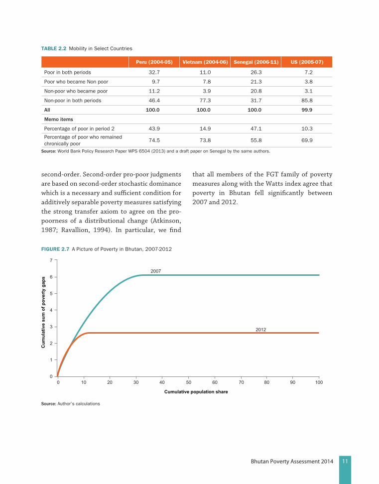
population escaping poverty as entering it. Bhutan’s upward mobility during 2007-2012 is comparable to Vietnam’s during 2004-06 (Table 2.2). Mobility for the bottom 40 percent in Bhutan is diminished compared to the poor group. Three-fourths of the bottom 40 percent remained in poverty whereas almost the same proportion (10 percent) of population left the bottom 40 percent and rejoined it between 2007 and 2012.
2.1.4. Growth in Bhutan has been Pro-Poor
Poverty reduction in Bhutan has been pro-poor. The change in the distribution of per capita expenditure between 2007 and 2012 can also be characterized by the growth incidence curve (Figure 2.9). Recall that this curve shows the growth rate of an indicator of the living standard (e.g., income or expenditure) at each quantile of the size distribution of that indicator (Ravallion and Chen, 2003). The fact that the GIC depicted in Figure 2.9 is greater than zero for all expenditure percentiles means that the distribution of per-capita expenditure in 2012 dominates the distribution in 2007 to the first order. In other words, it means the posterior
distribution of per-capita expenditure lies nowhere above the initial one. This first-order stochastic dominance relation between the two distributions implies that all additively separable poverty measures satisfying monotonicity4 will agree that poverty has decreased between 2007 and 2012. Thus, distributional change observed in Bhutan between those two years is pro-poor in the sense of Ravallion and Chen (2003) and Kray (2006). For these authors, a distributional change is pro-poor if it involves poverty reduction for some choice of poverty index.5
Growth has been pro-poor in a substantive way. The poverty implications of the above dis-tributional change are presented in Figure 2.7 that summarizes the variation in poverty out-comes in Bhutan between 2007 and 2012 on the basis of TIP curves associated with poverty measures that bare members of the FGT (Foster-Greer-Thorbecke) family. The TIP curve6provides a graphical summary of incidence, intensity and inequality dimensions of aggregate poverty based on the distribution of poverty gaps nor-malized by the poverty line7 (Jenkins and Lambert, 1997). The curve is obtained by par-tially cumulating individual contributions to overall poverty from the poorest individual to the richest.8 The fact that the TIP curve for 2007 lies above the 2012 curve suggests economic growth in Bhutan has been pro-poor to the
4 Monotonicity requires that, other things being equal, an increase in the living standard of any person will reduce poverty (Foster, Greer, and Thorbecke, 2010).
5 The fact that the rate of growth at every percentile up to the 92nd is less than the average annual growth rate of per-capita expenditure means that economic growth in Bhutan has not been pro-poor if it is defined to exceed the average growth for the entire population.
6 TIP stands for “three ‘i’s of poverty”, that is incidence, intensity, and inequality.
7 The curve may also be based on absolute poverty gaps.
8 This curve is constructed in four steps: (i) rank individuals from poorest to richest; (ii) compute the relative poverty gap of each individual; (iii) form the cumulative sum of the relative poverty gaps divided by population size; and (iv) plot the resulting cumulative sum of poverty gaps as a function of the cumulative population share.
TABlE 2.1 Mobility In and Out of Poverty between 2007 and 2012
Pov
erty
Sta
tus
2007
Poverty Status in 2012(Percentage distribution of population)
Poor non-Poor all
Poor 8.3 10.5 18.8
non-Poor 4.1 77.2 81.3
all 12.4 87.7 100.0
source: Staff estimates based on analysis of synthetic panel data constructed using cross-section data of Bhutan Living Standards Surveys 2007 and 2012. “Does a rising tide lift all boats? An investigation of the nexus between poverty reduction and poverty mobility in Bhutan in the late 2000s”, Hai-Anh, Pete Lanjouw, and T.G. Srinivasan, forthcoming.Note: The estimates here are from the synthetic panel, not reflecting the entire cross-section, and therefore they differ from poverty estimates of cross-section data used elsewhere.
11Bhutan Poverty Assessment 2014
second-order. Second-order pro-poor judgments are based on second-order stochastic dominance which is a necessary and sufficient condition for additively separable poverty measures satisfying the strong transfer axiom to agree on the pro-poorness of a distributional change (Atkinson, 1987; Ravallion, 1994). In particular, we find
that all members of the FGT family of poverty measures along with the Watts index agree that poverty in Bhutan fell significantly between 2007 and 2012.
TABlE 2.2 Mobility in Select Countries
Peru (2004-05) Vietnam (2004-06) Senegal (2006-11) uS (2005-07)
Poor in both periods 32.7 11.0 26.3 7.2
Poor who became Non poor 9.7 7.8 21.3 3.8
Non-poor who became poor 11.2 3.9 20.8 3.1
Non-poor in both periods 46.4 77.3 31.7 85.8
all 100.0 100.0 100.0 99.9
memo items
Percentage of poor in period 2 43.9 14.9 47.1 10.3
Percentage of poor who remained chronically poor
74.5 73.8 55.8 69.9
source: World Bank Policy Research Paper WPS 6504 (2013) and a draft paper on Senegal by the same authors.
FIguRE 2.7 A Picture of Poverty in Bhutan, 2007-2012
2007
2012
00
1
2
3
4
5
6
7
10 20 30 40 50 60 70 80 90 100
Cum
ulat
ive
sum
of p
over
ty g
aps
Cumulative population share
source: Author’s calculations
12 Bhutan Poverty Assessment 2014
2.2. stable Inequality
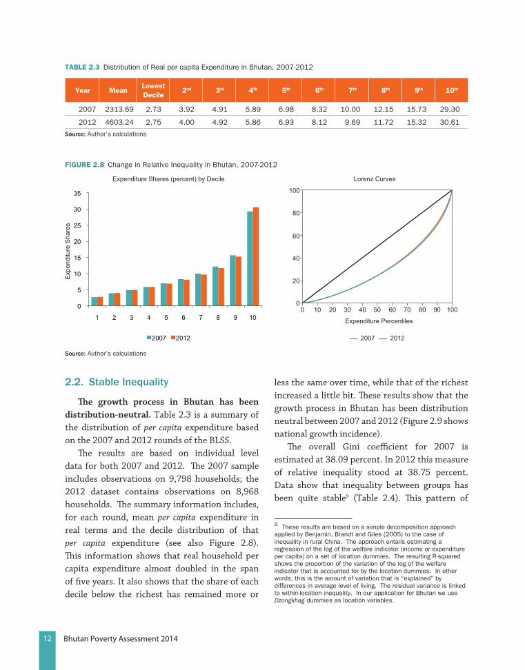
The growth process in Bhutan has been distribution-neutral. Table 2.3 is a summary of the distribution of per capita expenditure based on the 2007 and 2012 rounds of the BLSS.
The results are based on individual level data for both 2007 and 2012. The 2007 sample includes observations on 9,798 households; the 2012 dataset contains observations on 8,968 households. The summary information includes, for each round, mean per capita expenditure in real terms and the decile distribution of that per capita expenditure (see also Figure 2.8). This information shows that real household per capita expenditure almost doubled in the span of five years. It also shows that the share of each decile below the richest has remained more or
less the same over time, while that of the richest increased a little bit. These results show that the growth process in Bhutan has been distribution neutral between 2007 and 2012 (Figure 2.9 shows national growth incidence).
The overall Gini coefficient for 2007 is estimated at 38.09 percent. In 2012 this measure of relative inequality stood at 38.75 percent. Data show that inequality between groups has been quite stable9 (Table 2.4). This pattern of
9 These results are based on a simple decomposition approach applied by Benjamin, Brandt and Giles (2005) to the case of inequality in rural China. The approach entails estimating a regression of the log of the welfare indicator (income or expenditure per capita) on a set of location dummies. The resulting R-squared shows the proportion of the variation of the log of the welfare indicator that is accounted for by the location dummies. In other words, this is the amount of variation that is “explained” by differences in average level of living. The residual variance is linked to within-location inequality. In our application for Bhutan we use Dzongkhag dummies as location variables.
TABlE 2.3 Distribution of Real per capita Expenditure in Bhutan, 2007-2012
Year Meanlowest Decile
2nd 3rd 4th 5th 6th 7th 8th 9th 10th
2007 2313.69 2.73 3.92 4.91 5.89 6.98 8.32 10.00 12.15 15.73 29.30
2012 4603.24 2.75 4.00 4.92 5.86 6.93 8.12 9.69 11.72 15.32 30.61
source: Author’s calculations
FIguRE 2.8 Change in Relative Inequality in Bhutan, 2007-2012
00
20
40
60
80
100
10 20 30 40 50 60 70 80 90 100
Expenditure Percentiles
Lorenz CurvesExpenditure Shares (percent) by Decile
2007 2012
0
5
10
15
20
25
30
35
1 2 3 4 5 6 7 8 9 10
2007 2012
Exp
endi
ture
Sha
res
source: Author’s calculations

13Bhutan Poverty Assessment 2014
distributional change suggests that, overall, the observed reduction in poverty was driven exclusively by the size effect.
Inequality between dzongkhags remained stable in Bhutan. These results are based on a simple decomposition approach applied by Benjamin, Brandt and Giles (2005) to the case of inequality in rural China. The approach entails estimating a regression of the log of the welfare indicator (income or expenditure per capita) on a
set of location dummies. The resulting R-squared shows the proportion of the variation of the log of the welfare indicator that is accounted for by the location dummies. In other words, this is the amount of variation that is “explained” by differences in average level of living. The residual variance is linked to within-location inequality. In our application for Bhutan we use dzongkhag dummies as location variables.
2.2.1. uneven Poverty reduction across Dzongkhags
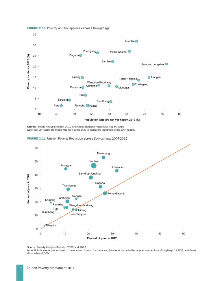
Incidences of unhappiness and poverty are higher in the eastern dzongkhags. The 2010 GNH survey estimates that 59 percent of Bhutanese are not-yet-happy; even in the least-poor Paro close to 47 percent are not-yet-happy. Using the national average for the percentage of poor in 2012 and not-yet-happy in 2010 as dividing lines (Figure 2.10), we note that unhappiness tends
TABlE 2.4 Between-Group (Dzongkhag) Inequality in Bhutan by Area of Residence
Year urban Rural Bhutan
2007 13.3 20.4 26.0
2012 14.5 22.4 25.0
source: Author’s calculationsNote: Between-group inequality is measured by the proportion of the variance of the log of per capita expenditure explained by dzongkhag of residence. This is the R2 of the regression of log per capita expenditure on a set of dummy variables representing the dzongkhag (see Benjamin and Brandt. 2005.“The Evolution of Income Inequality in Rural China.” Economic Development and Cultural Change).
FIguRE 2.9 Growth Incidence Curve for Bhutan, 2007-2012
12
14
16
18
20
22
24
0 10 20 30 40 50 60 70 80 90 100
Expenditure Percentiles
Ann
ual G
row
th R
ate
(%)
source: Author’s calculations
14 Bhutan Poverty Assessment 2014
FIguRE 2.11 Uneven Poverty Reduction across Dzongkhags, 2007-2012
Bumthang
Chhukha
Dagana
Haa
Lhuentse Monggar
Pema Gatshel
Punakha
Samdrup Jongkhar
Samtse
Sarpang
Trashigang
Trashi Yangtse
Trongsa
Tsirang
Wangdue Phodrang
Zhemgang
0
10
20
30
40
50
60
Perc
ent o
f poo
r in
2007
Percent of poor in 2012
Thimphu
source: Poverty Analysis Reports, 2007 and 2012Note: Bubble size is proportional to the number of poor. For instance, Samtse is home to the largest number for a dzongkhag, 12,000, and Pema Gatshelhas 6,000.
FIguRE 2.10 Poverty and Unhappiness across Dzongkhags
Bumthang
Chhukha
Dagana
Gasa
Haa
Lhuentse
Monggar
Paro
Pema Gatshel
Punakha
Samdrup Jongkhar Samtse
Sarpang
Thimphu
Trashigang
Trashi Yangtse Trongsa Tsirang
Wangdue Phodrang
Zhemgang
0
5
10
15
20
25
30
35
40 45 50 55 60 65 70 75 80
Pove
rty
Inci
denc
e 20
12 (%
)
Population who are not-yet-happy, 2010 (%)
source: Poverty Analysis Report 2012 and Gross National Happiness Report 2010Note: Not-yet-happy are those who lack sufficiency in indicators identified in the GNH report.
15Bhutan Poverty Assessment 2014
to increase with poverty and the eastern part of the country is highly prone to unhappiness and poverty.
Poverty reduction across dzongkhags has been uneven. Of the 20 dzongkhags in Bhutan, poverty reduction touched all except two, Pema Gatshel and Tsirang (Figure 2.11). The pace of poverty reduction was slower in Dagana and Lhuentse, but much faster in initially-very-poor Monggar, Samtse and Zhemgang. Even among the poor eastern dzongkhags, Zhemgang has been more successful than Lhuentse in poverty reduction.

17Bhutan Poverty Assessment 2014
Changing Profiles of the Poor and Bottom 40 Percent of the Population
This chapter presents the change in profiles of the poor and bottom 40 percent of the population between 2007 and 2012. The profiles are presented in terms of asset and amenities, health and nutrition, gender, and land ownership. This analysis complements discussion of the profile of the poor in Bhutan Poverty Analysis 2012.
3.1. Welfare Indicators (assets and amenities)
All non-consumption indicators of welfare showed significant improvements between 2007 and 2012, both for the general population and the poor (Table 3.1). Basic asset and amenity indi-cators used in BLSS survey years 2007 and 2012 show that the biggest improvements occurred in mobile phone ownership, housing, and electricity connections. In particular, there have been signi-ficant increases in the percentages of households with metal sheet roofs, electricity connections, and access to mobile phones. There has been a significant increase in the poorest households’ access to mobile phones and electricity. Improve-ment in their housing conditions, specifically in roof quality, has been dramatic.
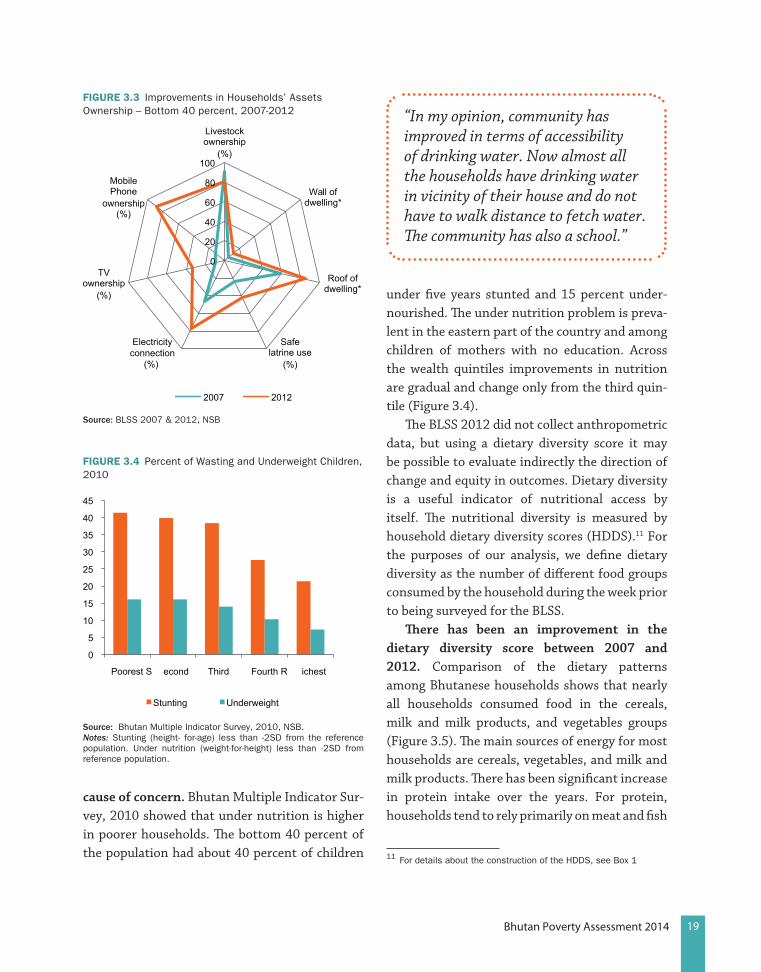
The improvements in households’ assets indicators are illustrated by the following three charts, in seven key dimensions of welfare –livestock ownership, type of dwelling wall, type of dwelling roof, safe latrine access, electricity access, television ownership, and access to mobile phone. For all households (Figure 3.1), between 2007 and 2012 there were improvements in six dimensions of welfare, except for livestock ownership which showed a small decline. The same pattern held true for the poorest households and those in the bottom four deciles of the real per-capita consumption distribution (Figures 3.2, 3.3). Both of these categories experienced relatively large improvements in asset ownership in the same six dimensions of welfare between 2007 and 2012, reflecting the ongoing pattern of improvement in asset accumulation in the country at large. By far the largest improvement in both the poorest households and those in the bottom four deciles was in mobile phone ownership – from 11 percent
3Chapter
“Mobile connectivity has also benefited us in communicating faster during emergencies.”

18 Bhutan Poverty Assessment 2014
in 2007 to 88 percent, in 2012, for the bottom four deciles. The increase in mobile phones among the poorest households was similarly dramatic. Other significant improvements for the poor came in electricity connections and the roofs of dwellings.
3.2. health and nutrition
Bhutan’s nutrition indicators have improved in recent years and are better now than in other South Asian countries, accord-ing to World Bank (2013),10 yet they remain a
10 Nutrition in Bhutan: Situational Analysis & Policy Recommendations, World Bank, 2013
TABlE 3.1 Trends in Basic Assets and Amenities, 2007-2012
All households Poor households Bottom 40 percent
2007 2012 2007 2012 2007 2012
Livestock ownership (%)1 59.6 51.8 93.0 86.9 90.3 80.7
Wall of dwelling* 22.3 26.4 3.3 6.1 5.3 12.1
Roof of dwelling** 74.0 89.3 53.4 78.8 58.7 84.4
Safe latrine use (%)2 48.2 62.0 21.1 32.8 23.5 41.7
Electricity connection (%)◊ 69.1 88.3 39.9 69.5 46.6 77.4
TV ownership (%) 37.7 58.5 6.4 21.6 8.8 33.3
Mobile Phone ownership (%) 39.3 92.8 6.6 81.7 11.2 87.8
source: BLSS 2007 and 2012Notes: * Percent with cement-bonded bricks/stone (external wall)** Percent with metal sheets (roof)◊Electricity % “from the grid”1Household ownership of livestock – specifically pigs, cattle, goat, buffaloes, horses, sheep, yaks, and poultry –is included in this category.2Percent of flush & pit latrine (2012). The safe latrine use consists of flush to piped sewer system, flush to septic tank (without soak pit); flush to septic tank (with soak pit) and flush to pit (latrine) in 2012, and flush toilet and pit latrine with septic tank in 2007. An “improved sanitation facility” is one that hygienically separates human excreta from human contact. (WHO, 2013) To assess whether the latrine used is safe or not, the type of toilet used by the households are identified in the BLSS for years 2012 and 2007.
FIguRE 3.1 Improvements in Households’ Assets Ownership – All Households, 2007-2012
0 20 40 60 80
100
Livestock ownership (%)
Wall of dwelling*
Roof of dwelling*
Safe latrine use (%)
Electricity connection (%)
TV ownership (%)
Mobile Phone ownership (%)
2007 2012
source: BLSS 2007 & 2012, NSB
FIguRE 3.2 Improvements in Households’ Assets Ownership – Poor Households, 2007-2012
0 20 40 60 80
100
Livestock ownership (%)
Wall of dwelling*
Roof of dwelling*
Safe latrine use (%)
Electricity connection (%)
TV ownership (%)
Mobile Phone ownership (%)
2007 2012
source: BLSS 2007 & 2012, NSB
19Bhutan Poverty Assessment 2014
cause of concern. Bhutan Multiple Indicator Sur-vey, 2010 showed that under nutrition is higher in poorer households. The bottom 40 percent of the population had about 40 percent of children
under five years stunted and 15 percent under-nourished. The under nutrition problem is preva-lent in the eastern part of the country and among children of mothers with no education. Across the wealth quintiles improvements in nutrition are gradual and change only from the third quin-tile (Figure 3.4).
The BLSS 2012 did not collect anthropometric data, but using a dietary diversity score it may be possible to evaluate indirectly the direction of change and equity in outcomes. Dietary diversity is a useful indicator of nutritional access by itself. The nutritional diversity is measured by household dietary diversity scores (HDDS).11 For the purposes of our analysis, we define dietary diversity as the number of different food groups consumed by the household during the week prior to being surveyed for the BLSS.
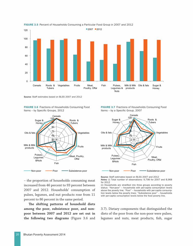
There has been an improvement in the dietary diversity score between 2007 and 2012. Comparison of the dietary patterns among Bhutanese households shows that nearly all households consumed food in the cereals, milk and milk products, and vegetables groups (Figure 3.5). The main sources of energy for most households are cereals, vegetables, and milk and milk products. There has been significant increase in protein intake over the years. For protein, households tend to rely primarily on meat and fish
11 For details about the construction of the HDDS, see Box 1
FIguRE 3.3 Improvements in Households’ Assets Ownership – Bottom 40 percent, 2007-2012
0
20
40
60
80
100
Livestock ownership
(%)
Wall of dwelling*
Roof of dwelling*
Safe latrine use
(%)
Electricityconnection
(%)
TV ownership
(%)
Mobile Phone
ownership (%)
2007 2012
source: BLSS 2007 & 2012, NSB
FIguRE 3.4 Percent of Wasting and Underweight Children, 2010
0
5
10
15
20
25
30
35
40
45
Poorest S econd Third Fourth R ichest
Stunting Underweight
source: Bhutan Multiple Indicator Survey, 2010, NSB.Notes: Stunting (height- for-age) less than -2SD from the reference population. Under nutrition (weight-for-height) less than -2SD from reference population.
“In my opinion, community has improved in terms of accessibility of drinking water. Now almost all the households have drinking water in vicinity of their house and do not have to walk distance to fetch water. The community has also a school.”
20 Bhutan Poverty Assessment 2014
– the proportion of households consuming meat increased from 46 percent to 93 percent between 2007 and 2012. Households’ consumption of pulses, legumes, and nut products rose from 11 percent to 86 percent in the same period.
The shifting patterns of household diets among the poor, subsistence poor, and non-poor between 2007 and 2012 are set out in the following two diagrams (Figure 3.6 and
3.7). Dietary components that distinguished the diets of the poor from the non-poor were pulses, legumes and nuts, meat products, fish, sugar
FIguRE 3.5 Percent of Households Consuming a Particular Food Group in 2007 and 2012
0
20
40
60
80
100
120 2007 2012
source: Staff estimates based on BLSS 2007 and 2012
FIguRE 3.6 Fractions of Households Consuming Food Items – by Specific Groups, 2012
50
60
70
80
90
100 Cereals
Roots & Tubers
Vegetables
Fruits
Meat, Poultry, Offal
Fish
Pulses, Legumes
&Nuts
Milk & Milk products
Oils & fats
Sugar & Honey
Non-poor Poor Subsistence poor
FIguRE 3.7 Fractions of Households Consuming Food Items – by a Specific Group, 2007
0
20
40
60
80
100 Cereals
Roots & Tubers
Vegetables
Fruits
Meat, Poultry, Offal
Fish
Pulses, Legumes
&Nuts
Milk & Milk products
Oils & fats
Sugar & Honey
Non-poor Poor Subsistence poor
source: Staff estimates based on BLSS 2007 and 2012 Notes: (i) Total number of observations: 9,798 for 2007 and 8,968 for 2012(ii) Households are stratified into three groups according to poverty status: “Non-poor” – households with per-capita consumption levels above the poverty line; “Poor” – households with per-capita consump-tion levels below the poverty lines; “Subsistence poor” – households with per-capita consumption levels below the food poverty line.
21Bhutan Poverty Assessment 2014
products, fruits, and milk and milk products. For three food groups – cereals, vegetables, oil and fats – no differences existed between the poor and non-poor in 2012, while there had been some distinction between them in 2007.
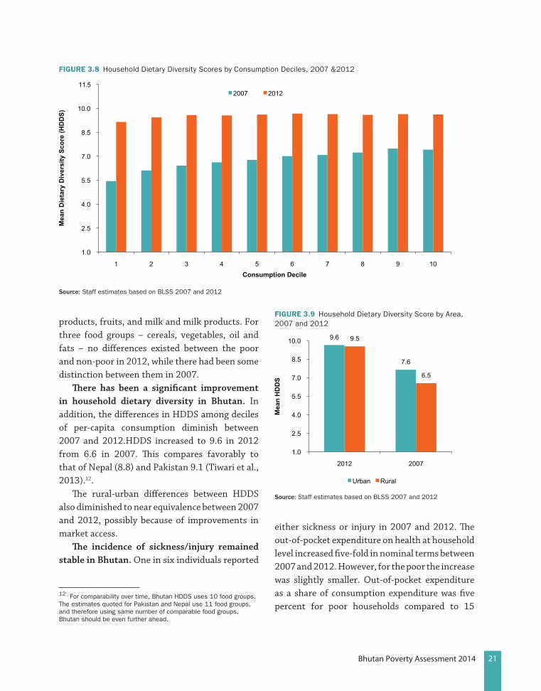
There has been a significant improvement in household dietary diversity in Bhutan. In addition, the differences in HDDS among deciles of per-capita consumption diminish between 2007 and 2012.HDDS increased to 9.6 in 2012 from 6.6 in 2007. This compares favorably to that of Nepal (8.8) and Pakistan 9.1 (Tiwari et al., 2013).12.
The rural-urban differences between HDDS also diminished to near equivalence between 2007 and 2012, possibly because of improvements in market access.
The incidence of sickness/injury remained stable in Bhutan. One in six individuals reported
12 For comparability over time, Bhutan HDDS uses 10 food groups. The estimates quoted for Pakistan and Nepal use 11 food groups, and therefore using same number of comparable food groups, Bhutan should be even further ahead.
either sickness or injury in 2007 and 2012. The out-of-pocket expenditure on health at household level increased five-fold in nominal terms between 2007 and 2012. However, for the poor the increase was slightly smaller. Out-of-pocket expenditure as a share of consumption expenditure was five percent for poor households compared to 15
FIguRE 3.9 Household Dietary Diversity Score by Area, 2007 and 2012
9.6
7.6
9.5
6.5
1.0
2.5
4.0
5.5
7.0
8.5
10.0
2012 2007
Mea
n H
DD
S
Urban Rural
source: Staff estimates based on BLSS 2007 and 2012
FIguRE 3.8 Household Dietary Diversity Scores by Consumption Deciles, 2007 &2012
1.0
2.5
4.0
5.5
7.0
8.5
10.0
11.5
1 2 3 4 5 6 7 8 9 10
Mea
n D
ieta
ry D
iver
sity
Sco
re (H
DD
S)
Consumption Decile
2007 2012
source: Staff estimates based on BLSS 2007 and 2012

22 Bhutan Poverty Assessment 2014
percent for non-poor households, indicative of the equity in access to health services.
3.3. Gender and Poverty
3.3.1. Is Poverty in Bhutan Gender-Blind?
The incidence of poverty in female-headed households was no different from that of male-headed households in 2012. But in 2007, the female-headed households fared better; the rate of decline in poverty incidence of male-headed households has been faster than those of females, to bring them level (Figure 3.10). The generally sanguine assessment of economic status of female-headed households may originate in the benefits ensuing from the matrilineal inheritance of land holdings, as noted in World Bank (2013).13 Comparison by marital status of the heads of households show heightened poverty incidence for female-headed households (compared to similarly placed male headed households) for the never-married, married, and divorced. Only for the widowed is the poverty incidence smaller (Table 3.2). A disproportionate burden of family chores, including child care by women, may restrict their choices to low-quality jobs even if there is no difference in rewards for labour. The higher poverty incidence for households headed by never-married females is puzzling, however.
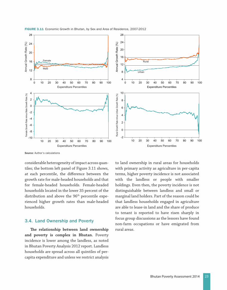
Male-headed and female-headed house-holds have experienced a reduction in poverty between 2007 and 2012 (Figure 3.11). The growth incidence curves by gender of heads of households (left panels) and by area (urban-rural) of resi-dence (right panels) show patterns of growth in each sub group similar to the overall pattern. One therefore would expect similar poverty outcomes. In particular, all additively separable poverty measures that satisfy both monotonicity and the transfer axiom will agree that male-headed
13 Bhutan Gender Policy Note, World Bank, 2013.
and female-headed households have experienced a reduction in poverty between 2007 and 2012. This is the case for urban and rural households as well.
There is a considerable heterogeneity of impact across quantiles. The information con-tained in Figure 3.11 reveals the following: The average annual growth rate of mean per capita expenditure is virtually the same for male-headed and female-headed households, but this hides
FIguRE 3.10 Trend in Poverty Incidence, by Gender of Household Head, 2007 and 2012
0
5
10
15
20
25
30
MHH MHH FHH FHH
2007 2012 2007 2012 Po
vert
y In
dice
nce
(%)
source: Staff estimates based on BLSS data
TABlE 3.2 Poverty Incidence in 2012, by Marital Status and Gender
2012
(Percentage of poor)
marital status male Female
Never married 3.7 10.5
Married 11.8 13.8
Divorced 4.4 6.2
Widower/widow 18.9 12.5
source: Staff estimates based on BLSS data
23Bhutan Poverty Assessment 2014
considerable heterogeneity of impact across quan-tiles; the bottom left panel of Figure 3.11 shows, at each percentile, the difference between the growth rate for male-headed households and that for female-headed households. Female-headed households located in the lower 35 percent of the distribution and above the 96th percentile expe-rienced higher growth rates than male-headed households.
3.4. Land ownership and Poverty
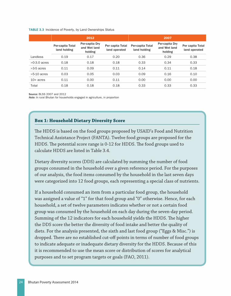
The relationship between land ownership and poverty is complex in Bhutan. Poverty incidence is lower among the landless, as noted in Bhutan Poverty Analysis 2012 report. Landless households are spread across all quintiles of per-capita expenditure and unless we restrict analysis
to land ownership in rural areas for households with primary activity as agriculture in per-capita terms, higher poverty incidence is not associated with the landless or people with smaller holdings. Even then, the poverty incidence is not distinguishable between landless and small or marginal land holders. Part of the reason could be that landless households engaged in agriculture are able to lease-in land and the share of produce to tenant is reported to have risen sharply in focus group discussions as the lessors have found non-farm occupations or have emigrated from rural areas.
FIguRE 3.11 Economic Growth in Bhutan, by Sex and Area of Residence, 2007-2012
8
12
16
20
24
28
0 10 20 30 40 50 60 70 80 90 100Expenditure Percentiles Expenditure Percentiles
Male
Female
Ann
ual G
row
th R
ate
(%)
Ann
ual G
row
th R
ate
(%)
Fema
le Gr
owth
Rate
minu
s Male
Gro
wth R
ate (%
)
Rura
l Gro
wth R
ate m
inus U
rban
Gro
wth R
ate (%
)
-10
-8
-6
-4
-2
0
2
4
10 20 30 40 50 60 70 80 90 100
4
8
12
16
20
24
28
0 10 20 30 40 50 60 70 80 90 100
Rural
Urban
-2
0
2
4
6
8
10
10 20 30 40 50 60 70 80 90 100
source: Author’s calculations
24 Bhutan Poverty Assessment 2014
TABlE 3.3 Incidence of Poverty, by Land Ownerships Status
2012 2007
Per-capita total
land holding
Per-capita Dry and Wet land
holding
Per capita total land operated
Per-capita total land holding
Per-capita Dry and Wet land
holding
Per capita total land operated
Landless 0.19 0.17 0.20 0.36 0.29 0.38
>0-3.0 acres 0.18 0.18 0.18 0.33 0.34 0.33
>3-5 acres 0.11 0.09 0.11 0.14 0.11 0.18
>5-10 acres 0.03 0.05 0.03 0.09 0.16 0.10
10+ acres 0.11 0.00 0.11 0.00 0.00 0.00
Total 0.18 0.18 0.18 0.33 0.33 0.33
source: BLSS 2007 and 2012Note: In rural Bhutan for households engaged in agriculture, in proportion
Box 1: Household Dietary Diversity Score
The HDDS is based on the food groups proposed by USAID’s Food and Nutrition Technical Assistance Project (FANTA). Twelve food groups are proposed for the HDDS. The potential score range is 0-12 for HDDS. The food groups used to calculate HDDS are listed in Table 3.4.
Dietary diversity scores (DDS) are calculated by summing the number of food groups consumed in the household over a given reference period. For the purposes of our analysis, the food items consumed by the household in the last seven days were categorized into 12 food groups, each representing a special class of nutrients.
If a household consumed an item from a particular food group, the household was assigned a value of “1” for that food group and “0” otherwise. Hence, for each household, a set of twelve parameters indicates whether or not a certain food group was consumed by the household on each day during the seven-day period. Summing of the 12 indicators for each household yields the HDDS. The higher the DDS score the better the diversity of food intake and better the quality of diets. For the analysis presented, the sixth and last food group (“Eggs & Misc.”) is dropped. There are no established cut-off points in terms of number of food groups to indicate adequate or inadequate dietary diversity for the HDDS. Because of this it is recommended to use the mean score or distribution of scores for analytical purposes and to set program targets or goals (FAO, 2011).

25Bhutan Poverty Assessment 2014
TABlE 3.4 Classification of Food Groups
Food group Number
Food group Name Examples
1 CEREALScorn/maize, rice, wheat, sorghum, millet or any other grains or foods made from these (e.g. bread, noodles, porridge or other grain products)
2 WHITE ROOTS AND TUBERSwhite potatoes, white yam, white cassava, or other foods made from roots
3
VITAMIN A RICH VEGETABLES AND TUBERS
pumpkin, carrot, squash, or sweet potato that are orange inside and other locally available vitamin A rich vegetables (e.g. red sweet pepper)
DARK GREEN LEAFY VEGETABLESdark green leafy vegetables, including wild forms and locally available vitamin A rich leaves such as amaranth, cassava leaves, kale, spinach
OTHER VEGETABLESother vegetables (e.g. tomato, onion, eggplant) and other locally available vegetables
4VITAMIN A RICH FRUITS
ripe mango, cantaloupe, apricot (fresh or dried), ripe papaya, dried peach, other locally available vitamin A rich fruits
OTHER FRUITS Other fruits, including wild fruits
5ORGAN MEAT liver, kidney, heart or other organ meats or blood-based foods
FLESH MEATSbeef, pork, lamb, goat, rabbit, game, chicken, duck, other birds, insects
6 EGGS eggs from chicken, duck, guinea fowl or any other egg
7 FISH AND SEAFOOD fresh or dried fish or shellfish
8 LEGUMES, NUTS AND SEEDSdried beans, dried peas, lentils, nuts, seeds or foods made from these (e.g., hummus, peanut)
9 MILK AND MILK PRODUCTS milk, cheese, yogurt or other milk products
10 OILS AND FATS oil, fats or butter added to food or used for cooking
11 SWEETSsugar, honey, sweetened soda or sweetened juice drinks, sugary foods such as chocolates, candies, cookies and cakes
12 SPICES, CONDIMENTS, BEVERAGESspices (black pepper, salt), condiments (soy sauce, hot sauce), coffee, tea, alcoholic beverages
source: FAO, 2011Notes: (i) The vegetable food group is a combination of vitamin A rich vegetables and tubers, dark green leafy vegetables and other vegetables(ii) The fruit group is a combination of vitamin A rich fruits and other fruits(iii) The meat group is a combination of organ meat and flesh meat


27Bhutan Poverty Assessment 2014
Enlarging Opportunities for Children
4.1. Inequality of opportunity in Bhutan
Research shows that access to a basic set of goods and services during childhood can be an important predictor of future outcomes. Access to quality basic services such as education, health care, and essential infrastructure (such as electricity, improved water, and sanitation), and early childhood development provides children the opportunity to advance and reach their potential, irrespective of their background. Equality of opportunity is about giving all children the same chance to succeed in life.
Equality of opportunity seeks to level the playing field so that circumstances such as sex, ethnicity, birthplace, or family background, which are beyond the control of an individual, do not influence a person’s life chances. Success in life should depend on people’s choices, effort, and talents, not their circumstances of birth. Reaching consensus on an agenda for reducing inequality of opportunity is politically more viable than trying to find agreement on redistributive policies to reduce inequality of income or wealth.
The Human Opportunity Index (HOI) is designed to gauge the progress of a country in equalizing opportunities for children in education. The HOI measures the availability of services that are necessary to progress in
life (such as education), discounted by how unequally the services are distributed between the different groups of the population. The HOI focuses exclusively on children, as opposed to the whole population, to endeavor to plot the course of poverty in the future. Analysis in this chapter
is restricted to educational outcomes and access to infrastructure. Health outcomes and early childhood development are not covered in the analysis because the BLSS data does not provide requisite data. Bhutan’s high GDP growth has been successful in realizing improved outcomes in education and infrastructure. Enrollments in primary and secondary are increasing and doing so at a faster rate than other countries with the same level of GDP per capita (Figure 4.2). At the same time, access to improved water sources and sanitation facilities have been increasing.Figure 4.1 illustrates how a low HOI in the past
4Chapter
“Most of the households have tap water for drinking. I have seen a lot of improvements related to health: improved cleanliness and sanitation.”
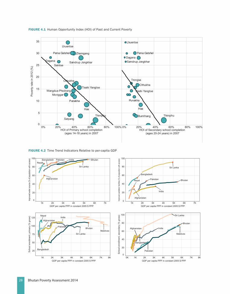
28 Bhutan Poverty Assessment 2014
FIguRE 4.1 Human Opportunity Index (HOI) of Past and Current Poverty
Thimphu
Haa
Samdrup Jongkhar
Trashi Yangtse
Punakha
Chhukha
Zhemgang
Wangdue Phodrang
Pema Gatshel
Sarpang
Lhuentse
Monggar
SamtseDagana
Thimphu
Haa
Samdrup Jongkhar
Chhukha
Bumthang
Trashi Yangtse
Pema Gatshel
Punakha
Trongsa
Lhuentse
Dagana
HOI of Primary school completion (ages 14-18 years) in 2007
Pov
erty
rate
in 2
012
(%)
HOI of Secondary school completion (ages 20-24 years) in 2007
0
5
10
15
20
25
30
35
0% 20% 40% 60% 80% 100% 0% 20% 40% 60% 80% 100%
FIguRE 4.2 Time Trend Indicators Relative to per-capita GDP
1K 2K 3K 4K 5K 6K 7KGDP per capita PPP in constant 2005 $ PPP
0
20
40
60
80
100
Impr
oved
sanit
ation
facil
ities (
% of
popu
lation
with
acce
ss)
Bangladesh
Nepal Pakistan
India
Afghanistan
Bhutan
Sri Lanka
1K 2K 3K 4K 5K 6K 7KGDP per capita PPP in constant 2005 $ PPP
0
20
40
60
80
100
Afghanistan
NepalBangladesh Pakistan India
Sri Lanka
Bhutan
Impr
oved
wate
r sou
rce (%
of po
pulat
ion w
ith ac
cess
)
1K 2K 3K 4K 5K 6K 7K 8KGDP per capita PPP in constant 2005 $ PPP
25
50
75
100
125
Sch
ool e
nrol
lmen
t, pr
imar
y (%
gro
ss)
Bhutan
Sri Lanka
Pakistan
AfghanistanIndia
Maldives
Nepal
Bangladesh
0K 1K 2K 3K 4K 5K 6K 7K 8KGDP per capita PPP in constant 2005 $ PPP
0
20
40
60
80
100
Sch
ool e
nrol
lmen
t, se
cond
ary
(% g
ross
)
Pakistan
Bhutan
Sri Lanka
Maldives
Bangladesh
Afghanistan India
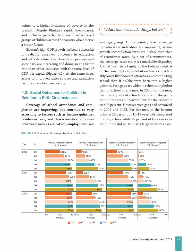
29Bhutan Poverty Assessment 2014
points to a higher incidence of poverty in the present. Despite Bhutan’s rapid, broad-based, and inclusive growth, there are disadvantaged groups of children across the country who deserve a better future.
Bhutan’s high GDP growth has been successful in realizing improved outcomes in education and infrastructure. Enrollments in primary and secondary are increasing and doing so at a faster rate than other countries with the same level of GDP per capita (Figure 4.2). At the same time, access to improved water sources and sanitation facilities have been increasing.
4.2. social outcomes for Children in relation to Birth Circumstances
Coverage of school attendance and com-pletion are improving, but continue to vary according to factors such as income quintiles, residences, sex, and characteristics of house-hold head such as education, employment, sex
and age group. At the country level, coverage for education indicators are improving, where growth incompletion rates are higher than that of attendance rates. By a set of circumstances, the coverage rates show a remarkable disparity. A child born to a family in the bottom quintile of the consumption distribution has a consider-ably lower likelihood of attending and completing school than if he/she were born into a higher quintile. Such gaps are wider in school completion than in school attendance. In 2003, for instance, the primary school attendance rate of the poor-est quintile was 50 percent, but for the richest it was 93 percent. However such gaps had narrowed in 2007 and 2012. For instance, in the bottom quintile 20 percent of 15-19 year-olds completed primary school while 75 percent of those in rich-est quintile did so. Similarly large variances exist
“Education has made things better.”
FIguRE 4.3 Education Coverage, by Wealth Quintiles
Year ByPrimary school attendance
(6-12 years)Primary school completion
(15-19 years)Secondary school attendance
(13-16 years)Secondary school completion
(20-24 years)
0% 50% 100%Coverage
0% 50% 100%Coverage
0% 50% 100%Coverage
0% 50% 100%Coverage
2003 Q1
Q2
Q3
Q4
Q5
2007 Q1
Q2
Q3
Q4
Q5
2012 Q1
Q2
Q3
Q4
Q5
50.5%
65.1%
76.7%
86.5%
92.6%
19.6%
31.4%
44.5%
63.4%
75.0%
35.1%
55.8%
73.3%
80.4%
85.3%
28.5%
40.4%
3.1%
5.3%
9.7%
71.3%
82.8%
89.8%
94.8%
97.4%
25.2%
45.4%
64.7%
75.2%
90.2%
55.4%
71.8%
82.1%
89.4%
92.8%
17.5%
27.7%
44.4%
68.0%
7.4%
90.8%
93.8%
96.4%
95.5%
97.9%
55.5%
64.5%
77.5%
83.2%
87.9%
82.5%
83.9%
89.6%
90.0%
93.6%
19.2%
30.6%
42.7%
55.2%
69.3%
Q1 Q2 Q3 Q4 Q5

30 Bhutan Poverty Assessment 2014
in urban and rural education, household heads’ levels of education, and employment.
While there are still notable gaps between school attendance and school completion among the various categories surveyed, those gaps have narrowed rapidly in the last decade (Figure 4.4).The illustration shows inequalities measured in terms ofratios betweentwo extreme categories in the same groups in the survey period. Each point represents the level of inequality by a specificcircumstance; for instance, the ratio of primary school attendance for children who are in the top quintile to that of the bottom quintile. First, it shows clearly that the levels of inequality have been reduced ineach of the four inequality ratios: children in the richest quintile vs.children in the poorest quintile; children in households with uneducated heads vs. children in households with secondary education; children in citiesvs.children in rural
areas; and children in households where the head is employed vs. those in households where the head is unemployed. Second, relationships between those indicators haveadjusted positively. For primary education, inequalities of attendance vs.completion have gonefrom about 1.8 and 3.7 respectively to roughly equal, at1.1 and 1.6, suggesting that there was an improvement in the transition from school attendance to school completion. The situation is also improving, but quitedifferently,insecondary education, where inequalities in school attendance are improving faster than those of completion. This suggests that the completion rates aremuch lower in secondary school than in primary school.
In addition, children typically are subject to multiple deprivations or disadvantages. Those multiple deprivations futher reduce opportunities in the long run. As shown in many instances, a child does not belong to a single group with
FIguRE 4.4 Multidimensional Inequalities of Education, 2003-2012
Primary school attendance (6-12 years)
1.0
1.5
2.0
2.5
3.0
3.5
4.0
Prim
ary
scho
ol c
ompl
etio
n (1
4-18
yea
rs)
Sec
onda
ry s
choo
l com
plet
ion
(20-
24 y
ears
)
2007
2003
20072012
2012
2007
2003
20032012
2012
2003
Secondary school attendance (13-16 years)
0
1
2
3
4
5
6
7
8
9
10
11
12
13
2007
2007
200720122012
2003
2007
2012
2003
2003
2012
2003
LegendQuintile - Q5/Q1Location - Urban/RuralEmployment - Yes/NoSecondary/No Education

31Bhutan Poverty Assessment 2014
FIguRE 4.5 Multiple Deprivations – Proportional Distribution of Children 6-12 years
2003 2007 2012
Distribution (%) Distribution (%) Distribution (%)
Gender Female Male
Location Rural Urban
WealthQuintiles
Q1 Q2 Q3 Q4 Q5
Group(UrbanQuintile)
Rural Q1 Rural Q2 Urban Q1 Urban Q2
Group(UrbanQuintileSex)
Rural Q1 Female Rural Q1 Male Rural Q2 Female Rural Q2 Male Urban Q1 Female Urban Q1 Male Urban Q2 Female Urban Q2 Male
50.9449.06
49.7950.21 50.67
49.33
82.7017.30 22.47
77.53 72.4027.60
24.3921.21
28.82
15.729.85
22.94
15.00
36.48
17.98
7.59
23.94
11.1016.91
27.62
20.42
22.6628.63
0.191.73
35.7620.48
2.460.72
26.3620.26
1.263.68
11.1711.49
15.2113.42
0.070.79
0.12
0.95
17.94
10.3410.14
17.82
1.171.29
0.310.41
13.4112.95
10.53
1.80
0.680.59
1.89
9.73
Multiple deprivations - Primary School Attendence (6-12 Years)
FIguRE 4.6 Multiple Deprivations – Proportional Distribution of Children 13-16 years
2003 2007 2012
Distribution (%) Distribution (%) Distribution (%)
Gender Fema le Ma le
Locati on Rural Urba n
WealthQuinti les
Q1 Q2 Q3 Q4 Q5
Group(UrbanQuinti le)
Rural Q1 Rural Q2 Urba n Q1 Urba n Q2
Group(UrbanQuinti leSex)
Rural Q1 Fem aleRural Q1 M aleRural Q2 Fem aleRural Q2 M aleUrba n Q1 Fem aleUrba n Q1 M aleUrba n Q2 Fem aleUrba n Q2 M ale
49.6950.31
51.5748.43 49.74
50.26
83.4516.55 22.87
77.13 74.0026.00
25.8019.41
28.02
16.2210.55
24.04
15.4610.16
31.10
19.2516.90
27.98
11.98
20.2122.93
27.8124.52
1.280.21
21.7630.51
2.280.59
26.8520.03
2.901.13
12.54
13.86
11.9713.95
0.67
0.09
0.61
0.12
15.40
10.7710.99
15.11
1.241.04
0.170.42
13.4713.38
10.33
1.44
9.70
1.47
0.580.55
Multiple deprivations - Secondary School Attendence (13-16 Years)

32 Bhutan Poverty Assessment 2014
disadvantaged circumstances, but to a variety ofsuch groups. For example, Figure 4.5 shows that among children aged 6-12 years in primary school in 2003, about 83 percent lived in rural areas, 29 percent were in the poorest quintile, and 15 percent were female. Such children, therefore,are have multiple disadvantages, and the numbers haverisen in the last decade. Thus, in cases of multiple deprivation the child’s access to opportunities such as education is signfinicantly worse than his or her peers who are subject to just a single deprivation or disadvantage. Whilethere are various differentiated contributions to the inequalities of circumstance, some factors might be more important than others.
There have been improvements in opportunities for access to infrastructure, specifically electricity, gas, and electricity for cooking. While the gender of the household head does not matter as much for infrastructure
provision, location of residence, education level of the household head, and wealth quintle index are important factors. Coverage of electricity,gas usage, and electricity for cooking acrossthe country depends on the location of the household (urban vs rural) as well as the education of the household head. Figure 4.7 shows the coverage of infrastructure indicators by education level of household head. It shows clearly that household heads with no education or primary or lesser education have a lower coverage rate of access to basic infrastructure than do households with heads with secondary or post-secondary education.
Coverage of infrastructure varies significantly in degree ofimprovement acrossthe country, and betweendifferent categories of circumstance during the survey period. In addition, overall inequalityiesas well as those of different categories of circumstances have been reducing in
FIguRE 4.7 Coverage of Basic Infrastructure, by Education of Household Head
Year By Access to electricityAccess to improvedprivate sanitation
Access to improvedsanitation
Access to improvedwater
Access to pipedwater
Using gas andelectricity for
cooking
0% 50% 100%Coverage
0% 50% 100%Coverage
0% 50% 100%Coverage
0% 50% 100%Coverage
0% 50% 100%Coverage
0% 50% 100%Coverage
2003 No Education
Primary
Secondary
Post-Secondary
2007 No Education
Primary
Secondary
Post-Secondary
2012 No Education
Primary
Secondary
Post-Secondary
33.2%
57.3%
89.3%
91.5%
78.8%
64.6%
71.5%
88.3% 100.0%
90.7%
95.7%
98.5%
80.8%
88.6%
97.8%
99.0%
78.6%
86.2%
97.8%
99.0%
18.8%
49.0%
84.4%
88.5%
63.8%
79.4%
94.7%
96.0%
80.9%
71.7%
73.3%
88.1%
94.9%
95.9%
99.3%
99.6%
88.4%
94.2%
98.2%
99.8%
87.3%
93.5%
98.1%
99.7%
45.1%
65.3%
91.5%
95.2%
87.6%
95.3%
98.3%
98.5%
67.4%
72.0%
78.2%
85.3%
73.7%
84.4%
94.7%
96.6%
97.6%
98.2%
99.0%
99.6%
96.3%
96.5%
98.3%
99.4%
78.6%
90.4%
97.3%
99.0%
No Education Primary Secondary Post-Secondary
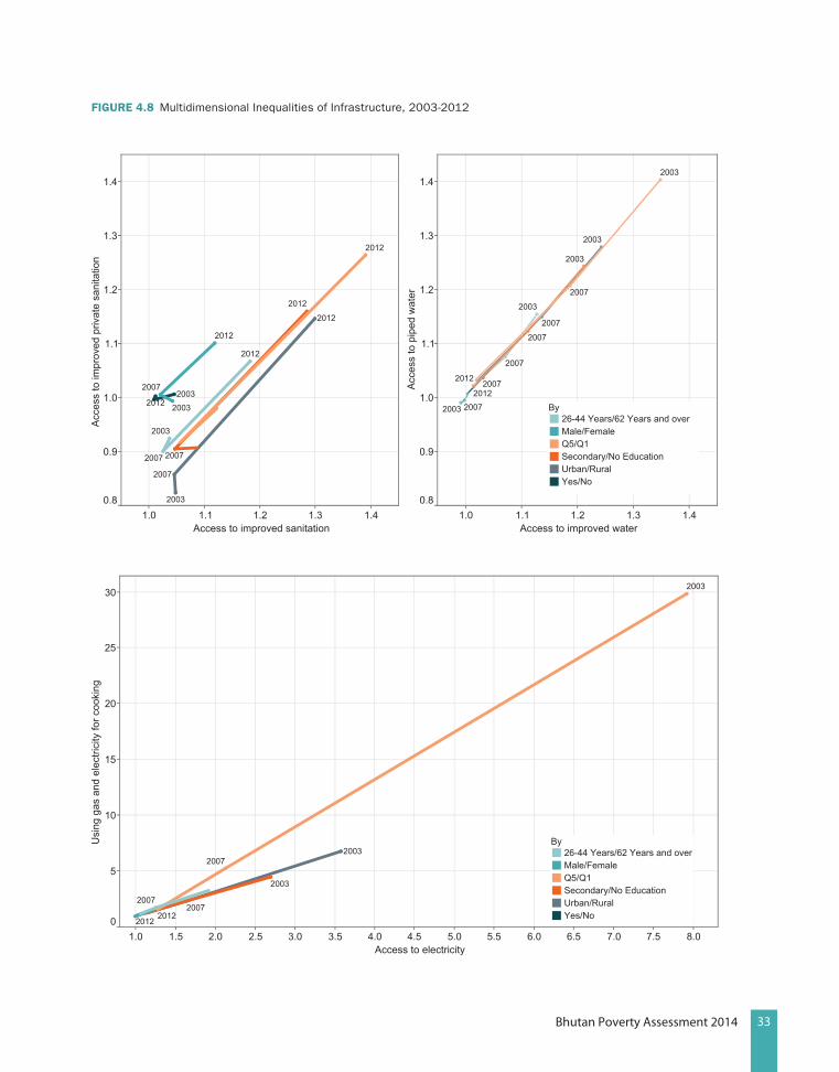
33Bhutan Poverty Assessment 2014
FIguRE 4.8 Multidimensional Inequalities of Infrastructure, 2003-2012
Access to improved water
0.8
0.9
1.0
1.1
1.2
1.3
1.4
Acc
ess
to p
iped
wat
er 2007
2007
2007
2007
2007
2007
2012
2003
2003
2012
2003
2003
2003
Access to improved sanitation
0.8
0.9
1.0
1.1
1.2
1.3
1.4
Acc
ess
to im
prov
ed p
rivat
e sa
nita
tion
2007
2007
2003
2003
2007
2007
2012
2012
2012
2003
2012
2012
20122003
By26-44 Years/62 Years and overMale/FemaleQ5/Q1Secondary/No EducationUrban/RuralYes/No
Access to electricity
0
5
10
15
20
25
30
Usi
ng g
as a
nd e
lect
ricity
for c
ooki
ng
2007
2012
2003
20072007
2003
2003
2012
By26-44 Years/62 Years and overMale/FemaleQ5/Q1Secondary/No EducationUrban/RuralYes/No
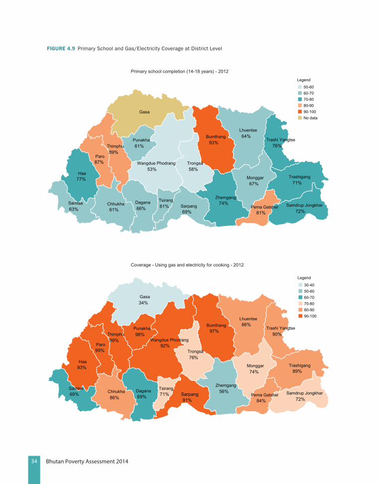
34 Bhutan Poverty Assessment 2014
FIguRE 4.9 Primary School and Gas/Electricity Coverage at District Level
53%
72%
76%
81%
71%
74%
93%
67%
64%
89%
61%
61%
69%
58%
66% 61%63%
77%
87% Wangdue Phodrang
Samdrup Jongkhar
Trashi Yangtse
Pema Gatshel
Trashigang
Zhemgang
Bumthang
Monggar
Lhuentse
Thimphu
Chhukha
Punakha
Sarpang
Trongsa
Dagana TsirangSamtse
Haa
Paro
Gasa
Primary school completion (14-18 years) - 2012
Legend
50-6060-7070-8080-9090-100No data
Wangdue Phodrang
Samdrup Jongkhar
Trashi Yangtse
Pema Gatshel
Trashigang
Zhemgang
Bumthang
Monggar
Lhuentse
Thimphu
Chhukha
Punakha
Trongsa
Dagana TsirangSamtse
Gasa
Haa
Paro 92%
72%
90%
84%
89%
56%
97%
74%
86%
99%
86%
98%
Sarpang91%
76%
69% 71%69%
34%
93%
99%
Coverage - Using gas and electricity for cooking - 2012
Legend
30-4050-6060-7070-8080-9090-100
35Bhutan Poverty Assessment 2014
this time. Figure 4.8 shows the multidimensional inequalities measured by the ratio of extremes in circumstances. There is a clear trend of significant decreasing inequalities between 2003 and 2012. For instance, the ratio of urban to rural for access to improved water has been reduced from around 1.2 to nearly 1.0, suggesting that households in urban and rural areas have nearly the same access to water. Inequalities in access towater and sanitation showsomewhat similar reduction rates. However, the indicators for electricity, gas and electricity for cooking shows clearly that not all households have the same, or any, access; inequalites are fourtimes higher in the same dimensions between access to electricity and using gas and electricity for cooking.
Across the country, the coverage of education and infrastructure varies significantly, with some district units performing relatively better than average at times. As Figure 4.9 shows, coverage for primary school completion rates were above 50 percent for all districts in 2012, but thatthe situationwas far worse for secondary schools at the district level. It is clear that in many districts Bhutan has made significant progress in meeting some MDGs foreducation, such as universal primary enrollment. In addition, reductions in poverty have also contributed to the progress of improvededucation indicators. However, those improvements are unequal atsub-national levels. Similarly, in the use of gas and electricty for cooking, coverage is highest in the middle of the country (more than 90 percent), a somewhat similar and the pattern to that of primary school completion.
4.3. measuring Inequality of opportunity
In order to analyze the variations in access across multiple circumstances, this paper makes use of the Human Opportunity Index (HOI). The HOI measures in a single indicator the coverage rate of a particular service, adjusted by how
equitably the available service is distributed among groups, differentiated by circumstances. This approach is more robust than traditional ones –looking at only one dimension, the strength of the approach lies in providing a single measure encapsulating both coverage and distribution of that coverage (Box 2).
The distribution of opportunity for children to access to education is improving in Bhutan. As indicated in Figure 4.10, the HOI for primary school attendance has increased significantly, reaching universal primary attendance where secondary school attendance is lower even though its coverage increased from 60 percent in 2003 to 87 percent in 2012. These results can be expected because the opportunity costs of sending children to school at these ages are much higher at the secondary than at the primary level. This also implies that some financial incentives, such as conditional cash transfer programs could be more effective in targeting older children to stay in school for learning longer.
Despite the high coverage for attendance, the story is much different for school completion: the HOI and coverage for school completion is far from universal. Besides the opportunity costs, there are other important and unobserved factors contributing to completing school, such as ability and determination.14 In addition, opportunities of children to access and complete secondary school or higher are much more limited, since the opportunities for them to move between grades or levels are low, especially for different groups across circumstances.
From the perspective of infrastructure, basic infrastructure services make significant contributions to wellbeing. Necessary services such as access to improved water and sanitation
14 It is important to note that the HOI provides a lower bound on the inequality prevalent in a given place, calculated by circumstances that are measurable and for which the data is available.

36 Bhutan Poverty Assessment 2014
Box 2: The Human Opportunity Index
The Human Opportunity Index (HOI) measures the availability of services that are necessary to progress in life (such as nutrition), discounted by how unequally the services are distributed among different groups in the population. Two countries that have identical coverage of nutrition services for infants, for instance, may have a different HOI if the infants that lack this service systematically share a personal circumstance beyond their control, such as gender, caste, parental income, or place of birth. Put simply, the HOI is coverage corrected for equity. In theory, it can be changed by providing more services to all (“scale effect”), or distributing services more fairly (“equalization effect”).
Calculating the HOIThe calculation of the HOI focuses on the dissimilarity index/inequality index, originally a demographic measure of evenness widely used in the analysis of social mobility, sociology in general and typically applied to dichotomous outcomes. Paes de Barro et al. (2009) define the dissimilarity index (D-index) as the weighted average of absolute differences of group-specific access rates (pi) from the overall average access rate (𝑝̅), or:
(1)
The D-index takes a value between 0 and 1. A value of zero indicates that access rates for all groups considered are the same, while positive values indicate that certain groups of individuals have a lower probability of access to the infrastructure service considered. In practical terms, the dissimilarity index reflects the percentage of the coverage rate of a particular opportunity that has to be discounted in order to obtain the HOI, i.e.,
(2)
As equation (2) shows, the HOI can be improved either by an increase in coverage (which is still bounded at 100 percent, universal access, and so the more people have access, the less likely that a particular segment of population is being left behind), or by a closer-to-zero dissimilarity index. At higher levels of coverage for a service, there is less room for unequal distribution of access across groups. However, the dissimilarity index, as we shall see, varies across opportunities and units of analysis, even at similar levels of coverage.
CaveatsIt is important to note that the HOI provides a lower bound on the inequality prevalent in a given place. Any calculation of the HOI can only include those circumstances that are measurable and for which data exist. Having a lower bound measure complicates comparison between countries or geographical regions, especially if the purpose is to investigate which country or region is more inequitable overall, and not which one has a lower minimum level of inequality.
Illustrating the HOI by ExampleConsider two countries, A and B, and consider a basic opportunity such as access to primary education. Suppose that in both countries, 50 percent of all children go to school. From the perspective of overall coverage, both countries look alike. Now suppose that in country A, no girl attends school, but in country B, 50 percent of both girls and boys attend school. The HOI discounts the coverage rate of 50 percent in country A through D since access is more unequal, based on the circumstance, gender. For country B, since there is no inequality based on gender, there is no discounting, making the HOI 50 percent, or equal to the coverage. Since country B has a higher HOI, it is more equal than country A, even though the average enrollment rate is the same in both countries.
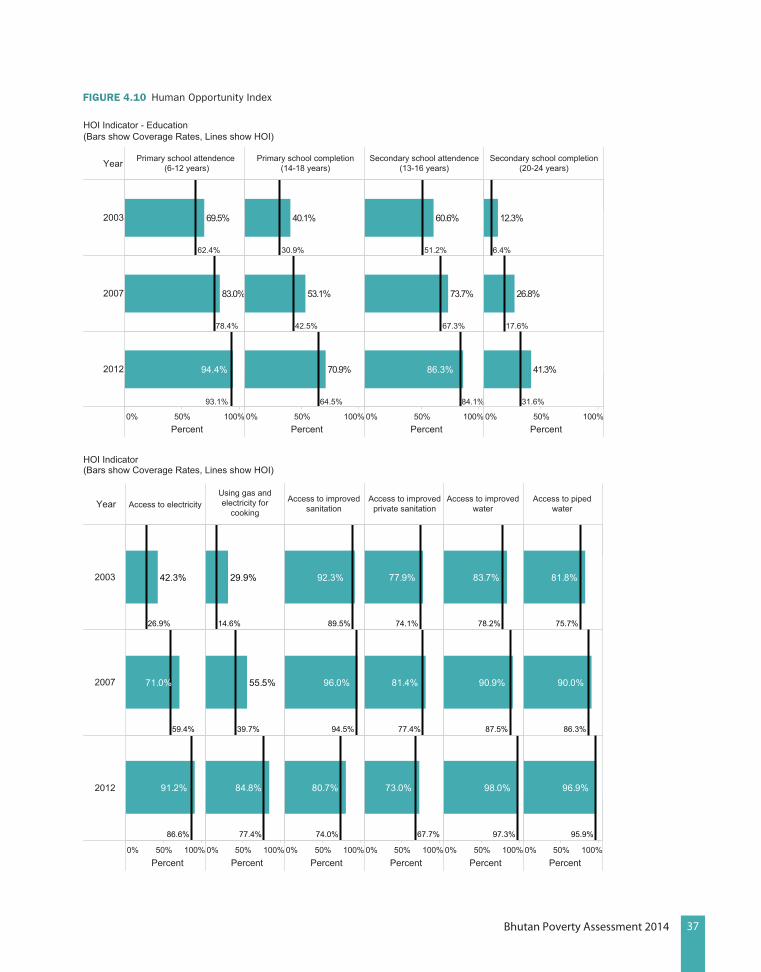
37Bhutan Poverty Assessment 2014
FIguRE 4.10 Human Opportunity Index
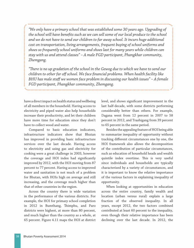
38 Bhutan Poverty Assessment 2014
have a direct impact on health status and wellbeing of all members in the household. Having access to electricity and piped water also help households increase their productivity, and let their children have more time for education since they don’t have to collect wood and water.
Compared to basic education indicators, infrastructure indicators show that Bhutan has improved in providing basic infrastructure services over the last decade. Having access to electricity and using gas and electricity for cooking were a great challenge in 2003, however the coverage and HOI index had significantly improved by 2012, with the HOI moving from 87 percent to 77 percent. Having access to improved water and sanitation is not much of a problem for Bhutan, with HOIs high on average and still increasing, and the coverage much higher than that of other countries in the region.
Across the country there is wide variation in the performance of the various districts. For example, the HOI for primary school completion in 2012 in Bumthang, Thimphu, and Paro districts were highest, at more than 80 percent, and much higher than the country as a whole, at 65 percent. Figure 4.11 maps the HOI at district
level, and shows significant improvement in the last half-decade, with some districts performing considerably better than others. For example, Dagana went from 12 percent in 2007 to 58 percent in 2012, and Trashigang from 39 percent to 65 percent in the same period.
Besides the appealing feature of HOI being able to summarize inequality of opportunity without tracking different circumstances one by one, the HOI framework also allows the decomposition of the contribution of particular circumstances, such as education of household heads and wealth quintile index overtime. This is very useful since individuals and households are typically characterized by a variety of circumstances, and it is important to know the relative importance of the various factors in explaining inequality of opportunity.
When looking at opportunities in education across the entire country, family wealth and location (urban versus rural) explain a large fraction of the observed inequality. In all years, except 2012, the two factors combined contributed at least 60 percent to the inequality, even though their relative importance has been declining over the last decade. In 2012, the
“We only have a primary school that was established some 30 years ago. Upgrading of the school will have benefits such as we can sell some of our local produce to the school and we do not have to send our children to far away school. It incurs huge additional cost on transportation, living arrangements, frequent buying of school uniforms and shoes so frequently school uniforms and shoes last for many years while children can stay with us and attend classes” – A male FGD participant, Phangkhar community, Zhemgang.
“There is no up gradation of the school in the Gewog due to which we have to send our children to other far off school. We face financial problems. When health facility like BHU has male staff we women face problem in discussing our health issues” – A female FGD participant, Phangkhar community, Zhemgang.
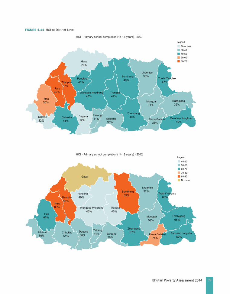
39Bhutan Poverty Assessment 2014
FIguRE 4.11 HOI at District Level
40%
49%
47%
38%
39%
40%
49%
31%
33%
67%
41%
41%
20%
35%
44%
12% 31%22%
56%
65% Wangdue Phodrang
Samdrup Jongkhar
Trashi Yangtse
Pema Gatshel
Trashigang
Zhemgang
Bumthang
Monggar
Lhuentse
Thimphu
Chhukha
Punakha
Sarpang
Trongsa
Dagana TsirangSamtse
Haa
Paro
Gasa
HOI - Primary school completion (14-18 years) - 2007
HOI - Primary school completion (14-18 years) - 2012
Legend
30 or less30-4040-5050-6060-70
45%
67%
68%
75%
65%
67%
89%
59%
52%
86%
51%
49%
59%
45%
58% 51%56%
65%
83% Wangdue Phodrang
Samdrup Jongkhar
Trashi Yangtse
Pema Gatshel
Trashigang
Zhemgang
Bumthang
Monggar
Lhuentse
Thimphu
Chhukha
Punakha
Sarpang
Trongsa
Dagana TsirangSamtse
Haa
Paro
Gasa
Legend
40-5050-6060-7070-8080-90No data
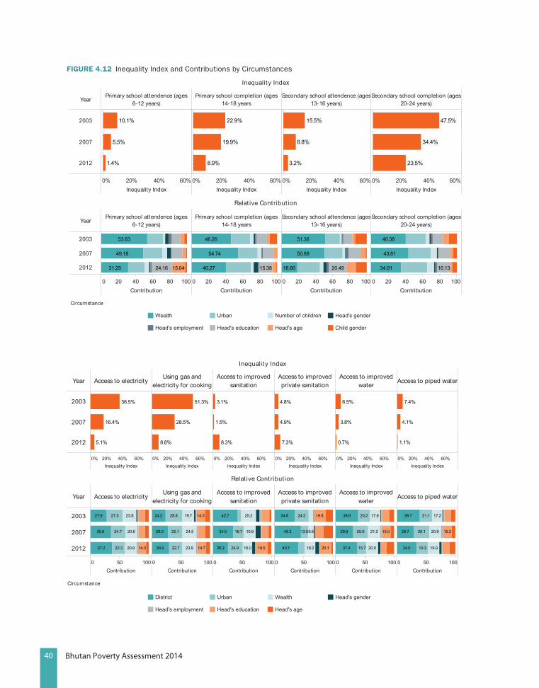
40 Bhutan Poverty Assessment 2014
FIguRE 4.12 Inequality Index and Contributions by Circumstances
YearPrimary school attendence (ages
6-12 years)Primary school completion (ages
14-18 yearsSecondary school attendence (ages
13-16 years)Secondary school completion (ages
20-24 years)
0% 20% 40% 60%Inequality Index
0% 20% 40% 60%Inequality Index
0% 20% 40% 60%Inequality Index
0% 20% 40% 60%Inequality Index
2003
2007
2012
10.1%
1.4%
5.5% 19.9%
22.9%
8.9%
15.5%
3.2%
8.8%
23.5%
34.4%
47.5%
Inequality Index
YearPrimary school attendence (ages
6-12 years)Primary school completion (ages
14-18 yearsSecondary school attendence (ages
13-16 years)Secondary school completion (ages
20-24 years)
0 20 40 60 80 100Contribution
0 20 40 60 80 100Contribution
0 20 40 60 80 100Contribution
0 20 40 60 80 100Contribution
2003
2007
2012 15.0424.16
49.18
31.25
53.83
54.74
46.26
40.27 15.38
51.36
18.66
50.68
20.49
40.38
43.81
34.91 16.13
Relat ive Contribut ion
Circumstance
Wealth Urban Number of children Head's gender
Head's employment Head's education Head's age Child gender
District Urban Wealth Head's gender
Head's employment Head's education Head's age
Year Access to electricityUsing gas and
electricity for cookingAccess to improved
sanitationAccess to improvedprivate sanitation
Access to improvedwater
Access to piped water
0% 20% 40% 60%Inequality Index
0% 20% 40% 60%Inequality Index
0% 20% 40% 60%Inequality Index
0% 20% 40% 60%Inequality Index
0% 20% 40% 60%Inequality Index
0% 20% 40% 60%Inequality Index
2003
2007
2012
36.5%
16.4%
5.1%
51.3%
28.5%
8.8%
3.1%
1.5%
8.3%
4.8%
4.9%
7.3%
6.5%
3.8%
0.7%
7.4%
4.1%
1.1%
Inequality Index
Year Access to electricityUsing gas and
electricity for cookingAccess to improved
sanitationAccess to improvedprivate sanitation
Access to improvedwater
Access to piped water
0 50 100Contribution
0 50 100Contribution
0 50 100Contribution
0 50 100Contribution
0 50 100Contribution
0 50 100Contribution
2003
2007
2012
20.635.6 24.7
23.8
20.9
27.9
14.237.2
27.3
22.3
28.0
14.7
19.7
22.7
28.8
23.929.9
25.1
24.2 14.5
24.5
16.0
18.7
42.7
19.9
24.9
25.2
26.2 19.5
34.5
34.6
13.0
40.7
19.8
20.118.2
24.3
45.3 9.6
37.4
15.0
20.015.7
17.8
29.8 25.9
38.9
21.2
20.2
34.0
39.7
29.7 20.9
19.9
21.1
26.1 15.2
17.2
19.3
Relat ive Contribut ion
Circumstance
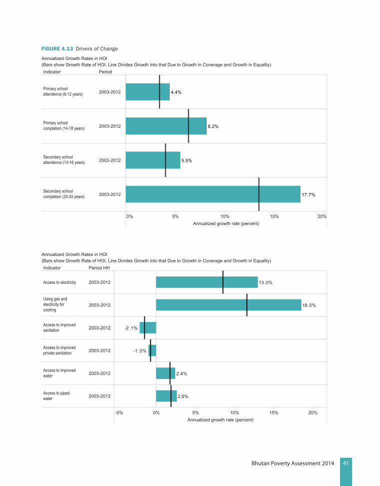
41Bhutan Poverty Assessment 2014
FIguRE 4.13 Drivers of Change
4.4%
8.2%
5.5%
17.7%
Indicator Period
0% 5% 10% 15% 20%Annualized growth rate (percent)
Primary schoolattendence (6-12 years) 2003-2012
Primary schoolcompletion (14-18 years) 2003-2012
Secondary schoolattendence (13-16 years) 2003-2012
Secondary schoolcompletion (20-24 years) 2003-2012
Annualized Growth Rates in HOI(Bars show Growth Rate of HOI, Line Divides Growth into that Due to Growth in Coverage and Growth in Equality)
13 .0%
18.5%
-2 .1%
-1 .0%
2.4%
2.6%
Indicator Period HH
Annualized growth rate (percent)
Access to electricity 2003-2012
Using gas and electricity forcooking
2003-2012
Access to improvedsanitation 2003-2012
Access to improvedprivate sanitation 2003-2012
Access to improvedwater 2003-2012
Access to pipedwater 2003-2012
Annualized Growth Rates in HOI(Bars show Growth Rate of HOI, Line Divides Growth into that Due to Growth in Coverage and Growth in Equality)

42 Bhutan Poverty Assessment 2014
contribution of a household head’s education is becoming an important factor, being now the third-largest contributor to unequal opportunities in education. Other factors that seem to matter include the number of children in the household, and children’s gender for secondary school attendance and completion. The fact that circumstances matter less and less for school attendance and completion across the country is good news. It speaks to the perspective of school universal policies over the last decade. Those policies are expanding and improving inputs, such as hiring quality teachers, and building more and better school infrastructure that ultimately close the gap of unreached population.
From the perspective of infrastructure, it is the location (district and urban/rural) and family wealth that explains over 70 percent of the inequality of opportunity across infrastructure indicators. This result is consistent with findings in other countries in the region, where factors of location and family wealth (measured by quintiles of per capita household expenditure) are the most important circumstances. For most indicators, the inequality index has declined significantly over the last decade, by four-to-six-fold, suggesting that access to basic infrastructure indicators is becoming more equal by different circumstances (from 36% to 5% for access to electricity and from 7% to 1% for access to piped water). This is due to an enabling environment that encourages
public or private investment in electricity and water services and projects –albeit that such environment exists mostly in urban areas.
4.4. Drivers of Change
For most opportunities in education and infrastructure the main driver of change has been increased coverage, but not much in the way of equity-enhancing programs. Figure 4.12 shows the annualized growth rates in HOI over the last decade; growth decomposable into growth in coverage and growth in equality. Notably, in education and infrastructure most of the growth in these indicators has come from “scale effect” improvements; in other words increased coverage, as opposed to the targeting of specific groups or circumstances. On the other hand, for access to electricity and use of gas and electricity for cooking indicators a significant proportion of the improvements in HOI has come from policies targeted at underserved groups rather than increased overall coverage, which indicates a more fair distribution of services (the so-called “equalization effect”).
The driver of change is much the same at the district level, where most of the HOI growth has come from growth in coverage. Figure 4.14 shows the HOI growth maps for primary school completion and access to electricity in 2007 and 2012. Numbers at the districts first denote growth of HOI, and secondly growth of coverage. It shows that in most of the districts there has been improvement in HOI, although there are still large variations in the magnitude of these improvements across districts. The figure also shows a large proportion of HOI growth has been due to coverage growth in spite of its unequal distribution.
“Before, we did not have electricity. Now after we received electricity wellbeing has improved. Road has also been connected. Before, we used horses to carry our loads. Previously we had to travel long way even to get kerosene for lighting purposes.”
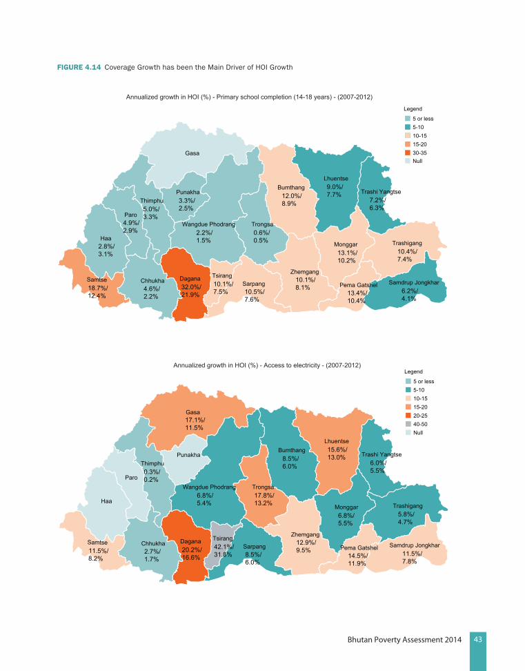
43Bhutan Poverty Assessment 2014
FIguRE 4.14 Coverage Growth has been the Main Driver of HOI Growth
2.2%/1.5%
6.2%/4.1%
7.2%/6.3%
13.4%/10.4%
10.4%/7.4%
10.1%/8.1%
12.0%/8.9%
13.1%/10.2%
9.0%/7.7%
5.0%/3.3%
4.6%/2.2%
3.3%/2.5%
10.5%/7.6%
0.6%/0.5%
32.0%/21.9%
10.1%/7.5%18.7%/
12.4%
2.8%/3.1%
4.9%/2.9%
Wangdue Phodrang
Samdrup Jongkhar
Trashi Yangtse
Pema Gatshel
Trashigang
Zhemgang
Bumthang
Monggar
Lhuentse
Thimphu
Chhukha
Punakha
Sarpang
Trongsa
Dagana TsirangSamtse
Haa
Paro
Gasa
Annualized growth in HOI (%) - Primary school completion (14-18 years) - (2007-2012)
Annualized growth in HOI (%) - Access to electricity - (2007-2012)
Legend
5 or less5-1010-1515-2030-35Null
6.8%/5.4%
17.1%/11.5%
11.5%/7.8%
6.0%/5.5%
14.5%/11.9%
5.8%/4.7%
12.9%/9.5%
8.5%/6.0%
6.8%/5.5%
15.6%/13.0%
0.3%/0.2%
2.7%/1.7%
8.5%/6.0%
17.8%/13.2%
20.2%/16.6%
42.1%/31.8%11.5%/
8.2%
Wangdue Phodrang
Samdrup Jongkhar
Trashi Yangtse
Pema Gatshel
Trashigang
Zhemgang
Bumthang
Monggar
Lhuentse
Thimphu
Chhukha
Punakha
Sarpang
Trongsa
Dagana TsirangSamtse
Haa
Paro
Gasa
Legend
5 or less5-1010-1515-2020-2540-50Null
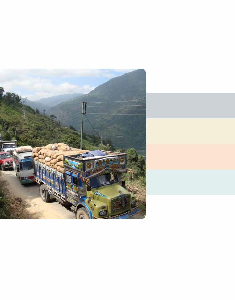

45Bhutan Poverty Assessment 2014
Key Drivers of Poverty Reduction in Bhutan
This chapter uses four alternative approaches to understanding the drivers of Bhutan’s rapid poverty reduction, since there is no direct, comparable data available on the sources of household income for two points in time. The first, economy-wide approach is to analyze the key factors that have driven growth and their potential pro-poor bias. The second approach is to construct a synthetic panel using cross-section data in the BLSS 2007 and 2012 to determine the profiles of people who escaped poverty. The third approach is to identify key drivers of change from an in-depth review of focus group discussions. Finally, an econometric estimation of welfare change at the percentile level is analyzed in order to shed light on the contribution from the accumulation of assets and returns on assets.
During 2007-2012, rapid poverty reduction has been driven mostly by growth in per-capita consumption expenditure than redistribution. For the whole of Bhutan, by every poverty measure, growth in per-capita consumption has been the dominant factor behind poverty reduction (Table 5.1). One notable exception is Pema Gatshel where growth was negative, but the reduction in inequality there largely compensated for this adverse effect. In Lhuentse and Trashi
5Chapter
“We have access to services like RNR. Through a group formation such as vegetable group has really helped us. Provision of services is mainly through technical assistance like marketing, harvesting, provision of seeds, fertilizers, etc.”
TABlE 5.1 Shapley Decomposition of Change in Poverty in Bhutan, 2007-2012
Overall growth Redistribution
headcount -11.16 -10.66 -0.05
Poverty Gap -3.45 -3.28 -0.06
squared Poverty Gap -1.38 -1.35 -0.05
Watts Index -4.50 -4.31 -0.01
Source: World Bank staff estimates
“At the household level over the last few years definitely there is improvement in income. Many households now sell dairy products in the local market although it may be in small quantity.”
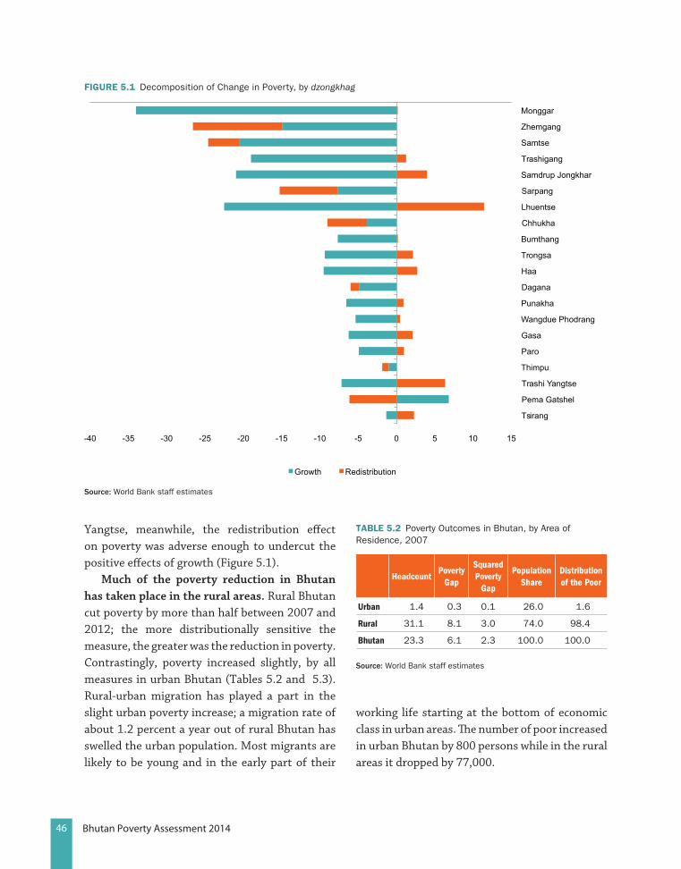
46 Bhutan Poverty Assessment 2014
Yangtse, meanwhile, the redistribution effect on poverty was adverse enough to undercut the positive effects of growth (Figure 5.1).
Much of the poverty reduction in Bhutan has taken place in the rural areas. Rural Bhutan cut poverty by more than half between 2007 and 2012; the more distributionally sensitive the measure, the greater was the reduction in poverty. Contrastingly, poverty increased slightly, by all measures in urban Bhutan (Tables 5.2 and 5.3). Rural-urban migration has played a part in the slight urban poverty increase; a migration rate of about 1.2 percent a year out of rural Bhutan has swelled the urban population. Most migrants are likely to be young and in the early part of their
working life starting at the bottom of economic class in urban areas. The number of poor increased in urban Bhutan by 800 persons while in the rural areas it dropped by 77,000.
FIguRE 5.1 Decomposition of Change in Poverty, by dzongkhag
Monggar
Zhemgang
Samtse
Trashigang
Samdrup Jongkhar
Sarpang
Lhuentse
Chhukha
Bumthang
Trongsa
Haa
Dagana
Punakha
Wangdue Phodrang
Gasa
Paro
Thimpu
Trashi Yangtse
Pema Gatshel
Tsirang
Growth Redistribution
source: World Bank staff estimates
TABlE 5.2 Poverty Outcomes in Bhutan, by Area of Residence, 2007
HeadcountPoverty
Gap
Squared Poverty
Gap
Population Share
Distribution of the Poor
Urban 1.4 0.3 0.1 26.0 1.6
Rural 31.1 8.1 3.0 74.0 98.4
Bhutan 23.3 6.1 2.3 100.0 100.0
source: World Bank staff estimates

47Bhutan Poverty Assessment 2014
Since most poverty reduction has been driven by growth and took place in the rural areas (93 percent, with the population shift to lower-poverty urban areas contributing 13 percent15), we examine, in the rest of this chapter, the factors that could have been responsible for the transformation of the rural sector.
Most rural households in the bottom quintile now rank wages and salaries as their main source of income. It appears that most of the employment expansion in the rural sector has been pro-poor. In the bottom quintile, there has been a dramatic shift in the main income source between 2007 and 2012. While own farm enterprise was identified by the bottom quintile
15 The interaction term increased poverty by 6 percent.
as the main source of income in 2007, by 2012 it had shifted to wages and salaries, although we cannot distinguish if this came from agriculture or non-agriculture sectors.
There are three key drivers behind the dynamism of rural Bhutan: increasing agricultural trade, expanding road networks, and spreading spillovers from hydroelectric projects.
5.1. trading out of Poverty
Despite the limited land available for cultivation, land productivity in value terms has been rising in Bhutan. Bhutan has less than 3 percent of land area under cultivation, and this may have been decreasing.16However, crop production per land area has been rising in constant prices. The FAO (2014) estimates 8 percent annual growth in crop production per hectare over 2006 to 2011, on top of a 7 percent annual increase over the preceding five-year period.17Moreover, real GDP from agriculture shows lackluster growth over the same period. With production shifting fast to high-value crops, the GDP for agriculture which is based on 2000 figures, is likely to underestimate the real GDP contribution from agriculture.
A shift to high-value commercial crops has been an important reason for the rise in production value per acre. Spurred by trade agreements with India and Bangladesh, Bhutan has been shifting to crops more suited to its comparative advantage. The area under cereals has been on the decline with substitution by fruit and vegetable crops. Further, the commercial
16 A time-trend for cultivated areas is hard to assess because assessment methodology has improved. Factors such as fluctuation in snow cover, urbanization, and fallowing of tseri land have also contributed to the altering of land-cover figures, according to the Land Cover Mapping Project, Ministry of Agriculture and Forests, 2010.
17 FAOSTAT country profile for Bhutan was accessed on February 7, http://faostat.fao.org/site/666/default.aspx
TABlE 5.3 Poverty Outcomes in Bhutan, by Area of Residence, 2012
HeadcountPoverty
Gap
Squared Poverty
Gap
Population Share
Distribution of the Poor
urban 1.8 0.3 0.1 34.0 3.1
rural 16.7 3.6 1.2 66.0 96.9
Bhutan 12.0 2.6 0.9 100.0 100.0
source: World Bank staff estimates
TABlE 5.4 Bottom Quintile’s First-Ranked Income Source (Percentage of Rural Households)
2007 2012
Wages and salaries 18.5 41.5
own business 4.8 8.1
own farm 63.5 34.3
remittance 2.1 6.8
Pension 0.0 0.3
real estate / rent 2.1 0.4
all others 9.0 8.5
100.0 100.0
source: World Bank staff estimates
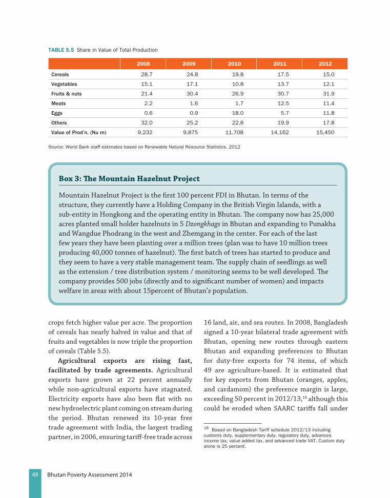
48 Bhutan Poverty Assessment 2014
crops fetch higher value per acre. The proportion of cereals has nearly halved in value and that of fruits and vegetables is now triple the proportion of cereals (Table 5.5).
Agricultural exports are rising fast, facilitated by trade agreements. Agricultural exports have grown at 22 percent annually while non-agricultural exports have stagnated. Electricity exports have also been flat with no new hydroelectric plant coming on stream during the period. Bhutan renewed its 10-year free trade agreement with India, the largest trading partner, in 2006, ensuring tariff-free trade across
16 land, air, and sea routes. In 2008, Bangladesh signed a 10-year bilateral trade agreement with Bhutan, opening new routes through eastern Bhutan and expanding preferences to Bhutan for duty-free exports for 74 items, of which 49 are agriculture-based. It is estimated that for key exports from Bhutan (oranges, apples, and cardamom) the preference margin is large, exceeding 50 percent in 2012/13,18 although this could be eroded when SAARC tariffs fall under
18 Based on Bangladesh Tariff schedule 2012/13 including customs duty, supplementary duty, regulatory duty, advances income tax, value added tax, and advanced trade VAT. Custom duty alone is 25 percent.
TABlE 5.5 Share in Value of Total Production
2008 2009 2010 2011 2012
Cereals 28.7 24.8 19.8 17.5 15.0
vegetables 15.1 17.1 10.8 13.7 12.1
Fruits & nuts 21.4 30.4 26.9 30.7 31.9
meats 2.2 1.6 1.7 12.5 11.4
eggs 0.6 0.9 18.0 5.7 11.8
others 32.0 25.2 22.8 19.9 17.8
value of Prod’n. (nu m) 9,232 9,875 11,708 14,162 15,450
Source: World Bank staff estimates based on Renewable Natural Resource Statistics, 2012
Box 3: The Mountain Hazelnut Project
Mountain Hazelnut Project is the first 100 percent FDI in Bhutan. In terms of the structure, they currently have a Holding Company in the British Virgin Islands, with a sub-entity in Hongkong and the operating entity in Bhutan. The company now has 25,000 acres planted small holder hazelnuts in 5 Dzongkhags in Bhutan and expanding to Punakha and Wangdue Phodrang in the west and Zhemgang in the center. For each of the last few years they have been planting over a million trees (plan was to have 10 million trees producing 40,000 tonnes of hazelnut). The first batch of trees has started to produce and they seem to have a very stable management team. The supply chain of seedlings as well as the extension / tree distribution system / monitoring seems to be well developed. The company provides 500 jobs (directly and to significant number of women) and impacts welfare in areas with about 15percent of Bhutan’s population.
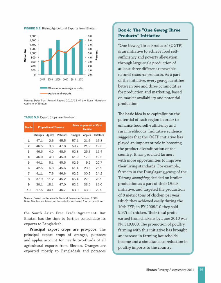
49Bhutan Poverty Assessment 2014
the South Asian Free Trade Agreement. But Bhutan has the time to further consolidate its exports to Bangladesh.
Principal export crops are pro-poor. The principal export crops of oranges, potatoes and apples account for nearly two-thirds of all agricultural exports from Bhutan. Oranges are exported mostly to Bangladesh and potatoes
TABlE 5.6 Export Crops are Pro-Poor
Decile Proportion of FarmersSales as percent of Cash
Income
Oranges Apples Potatoes Oranges Apples Potatoes
1 47.1 2.6 45.5 57.1 21.6 16.8
2 46.5 3.6 47.8 59.7 21.9 19.3
3 46.6 4.0 48.6 62.8 26.3 19.4
4 46.0 4.3 45.9 61.9 17.6 19.5
5 44.1 5.1 45.5 62.9 9.5 20.7
6 42.5 6.8 45.6 61.4 23.5 25.9
7 41.1 7.6 46.6 62.2 30.5 24.2
8 37.9 11.2 45.2 65.4 27.9 28.9
9 30.1 18.1 47.0 62.2 33.5 32.0
10 17.5 34.1 46.7 63.0 43.0 29.9
source: Based on Renewable Natural Resource Census, 2008Note: Deciles are based on household-purchased food expenditure.
Box 4: The “One Gewog Three Products” Initiative
“One Gewog Three Products” (OGTP) is an initiative to achieve food self-sufficiency and poverty alleviation through large-scale production of at least three different renewable natural resource products. As a part of the initiative, every gewog identifies between one and three commodities for production and marketing, based on market availability and potential production.
The basic idea is to capitalize on the potential of each region in order to enhance food self-sufficiency and rural livelihoods. Indicative evidence suggests that the OGTP initiative has played an important role in boosting the product diversification of the country. It has provided farmers with more opportunities to improve their living standards. For example, farmers in the Dunglagang gewog of the Tsirang dzongkhag decided on broiler production as a part of their OGTP initiative, and targeted the production of 8 metric tons of chicken per year, which they achieved easily during the 10th FYP; in FY 2009/10 they sold 9.97t of chicken. Their total profit earned from chickens by June 2010 was Nu 319,800. The promotion of poultry farming with this initiative has brought an increase in farming households’ income and a simultaneous reduction in poultry imports to the country.
FIguRE 5.2 Rising Agricultural Exports from Bhutan
0.0 1.0 2.0 3.0 4.0 5.0 6.0 7.0 8.0 9.0
0 200 400 600 800
1,000 1,200 1,400 1,600 1,800
2007 2008 2009 2010 2011 2012
Perc
ent
Mill
ion
Nu
Share of non-energy exports
Agricultural exports
source: Data from Annual Report 2012/13 of the Royal Monetary Authority of Bhutan

50 Bhutan Poverty Assessment 2014
to India. Among these crops, half or more of the farmers in poorer deciles grow oranges and potatoes, with apples a distant third. A significant share of the cash income of the farmers in poorer deciles is sourced from these export crops (Table 5.6), with orange farmers in poorer deciles reaping close to 60 percent of their cash income from the crop. The poverty incidence has fallen sharply, with close to 50 percent of households engaged in agriculture, second only to those engaged in construction.
The 10th Five Year Plan has been an important aid to the agricultural sector. The strategies of the plan give impetus to the commercial orientation of agriculture by aiming to:
a. Enhance sustainable rural livelihoods through improved agricultural and live-stock productivity and expansion of commercial prospects of agriculture and other natural resource endowments;
a. Conserve and promote sustainable com-mercial utilization of forest and water resources;
b. Promote sustainable utilization of arable agriculture and pasture land resources;
c. Enhance food security through sustain-able and enhanced food production and availability, improved access to food and enabling effective distribution, market-ing and import of food; and
d. Transform subsistence agriculture to small-scale commercial agriculture with-out compromising food security. “One Gewog Three Products” (OGTP) is a declared policy to diversify production activities at the gewog level (Box 4).
5.2. roads out of Poverty
International evidence on the impact of rural roads on poverty is positive, although attribution problems need to be handled
carefully. High quality rural roads reduce poverty, raise consumption, provide access to off-farm jobs, and increase school enrolment and completion rates (Dercon et al., 2009; Yamauchi et al., 2009). Khandker et al. (2009) investigated the impacts of rural road projects using household-level panel data from Bangladesh. Findings suggest that rural road investments reduce poverty significantly through higher agricultural production, higher wages, lower input and transportation costs, and higher output prices. Rural poverty incidence in Laos declined by 9.5 percent of the rural population between 1997/98 and 2002/03, and approximately 13 percent of this decline can be attributed to improved road access (Warr, 2010). The road investment gains were reported proportionately higher for the poor than for the non-poor, in other words road investments are pro-poor. Evidence from Sri Lanka, Indonesia, and the Philippines confirm that the poor and very poor benefit, substantially so, from rural roads (Hettige, 2006). In India, the expenditure on roads was found to have the largest impact on rural poverty compared to other types of public expenditure. For every 1 million rupees (US$22,000) invested in rural roads, 163 people were lifted out of poverty. In Vietnam, for every dong invested in roads, the value of agricultural production would increase by three dongs (World Bank, 2010).
Bhutan embarked on big programs of road infrastructure building in the 10th Five Year Plan (2008-2013). There were two initiatives in the road sector one from the Ministry of Works and Human Settlement and the other on rural access under the Ministry of Agriculture and Forests:
a. Ensure that 85 percent of the rural population lives within a half-day’s walk from the nearest road;
b. Connect Phuentsholing to Samtse thro-ugh the Southern East-West Highway;
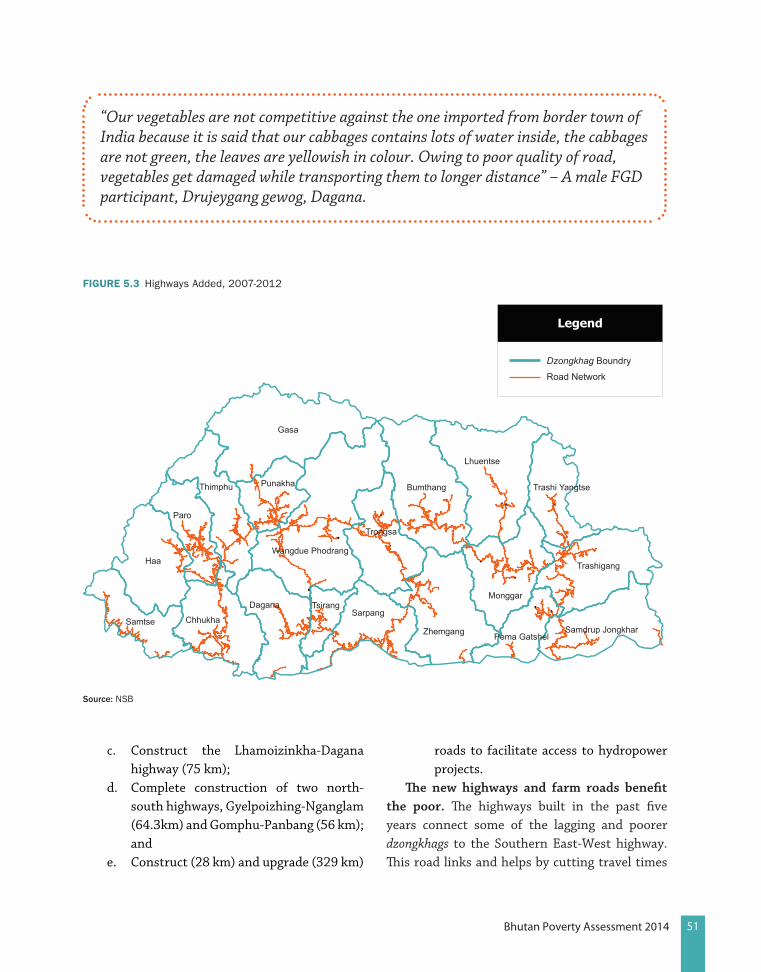
51Bhutan Poverty Assessment 2014
c. Construct the Lhamoizinkha-Dagana highway (75 km);
d. Complete construction of two north-south highways, Gyelpoizhing-Nganglam (64.3km) and Gomphu-Panbang (56 km); and
e. Construct (28 km) and upgrade (329 km)
roads to facilitate access to hydropower projects.
The new highways and farm roads benefit the poor. The highways built in the past five years connect some of the lagging and poorer dzongkhags to the Southern East-West highway. This road links and helps by cutting travel times
“Our vegetables are not competitive against the one imported from border town of India because it is said that our cabbages contains lots of water inside, the cabbages are not green, the leaves are yellowish in colour. Owing to poor quality of road, vegetables get damaged while transporting them to longer distance” – A male FGD participant, Drujeygang gewog, Dagana.
FIguRE 5.3 Highways Added, 2007-2012
Dzongkhag Boundry
Road Network
Gasa
Paro
Haa
Samtse Chhukha
Dagana TsirangSarpang
Trongsa
Bumthang
Lhuentse
Trashi Yangtse
Pema Gatshel
Trashigang
Samdrup Jongkhar
Monggar
Zhemgang
Wangdue Phodrang
PunakhaThimphu
source: NSB
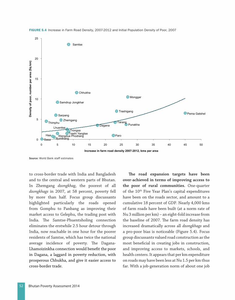
52 Bhutan Poverty Assessment 2014
to cross-border trade with India and Bangladesh and to the central and western parts of Bhutan. In Zhemgang dzongkhag, the poorest of all dzongkhags in 2007, at 58 percent, poverty fell by more than half. Focus group discussants highlighted particularly the roads opened from Gomphu to Panbang as improving their market access to Gelephu, the trading post with India. The Samtse-Phuentsholing connection eliminates the erstwhile 2.5 hour detour through India, now reachable in one hour for the poorer residents of Samtse, which has twice the national average incidence of poverty. The Dagana-Lhamoizinkha connection would benefit the poor in Dagana, a laggard in poverty reduction, with prosperous Chhukha, and give it easier access to cross-border trade.
The road expansion targets have been over-achieved in terms of improving access to the poor of rural communities. One-quarter of the 10th Five Year Plan’s capital expenditures have been on the roads sector, and amount to a cumulative 18 percent of GDP. Nearly 4,000 kms of farm roads have been built (at a norm rate of Nu 3 million per km) – an eight-fold increase from the baseline of 2007. The farm road density has increased dramatically across all dzongkhags and a pro-poor bias is noticeable (Figure 5.4). Focus group discussants valued road construction as the most beneficial in creating jobs in construction, and improving access to markets, schools, and health centers. It appears that per km expenditure on roads may have been less at Nu 1.5 per km thus far. With a job-generation norm of about one job
FIguRE 5.4 Increase in Farm Road Density, 2007-2012 and Initial Population Density of Poor, 2007
Chhukha
Haa
Monggar
Paro
Pema Gatshel
Punakha
Samdrup Jongkhar
Samtse
Sarpang Trashigang
Zhemgang
0
5
10
15
20
25
0 5 10 15 20 25 30 35 40 45 50
Den
sity
of p
oor,
num
ber p
er a
rea
(Sq
km)
Increase in farm road density 2007-2012, kms per area
Trongsa Trashi Yangtse
Wangdue Phodrang
Thimphu
Gasa
Tsirang
Bumthang
Lhuentse Dagana
source: World Bank staff estimates

53Bhutan Poverty Assessment 2014
for every US$1500 US$19 spent, the cumulative short-term jobs created could be around 65,000 between 2007 and 2012. It is likely that much of the job generation could have benefited to Bhutanese labour local to the communities. It is also likely that working age poor could have been taken on the manual labour of road construction.
5.3. the hydro effect
Spillover effects from hydroelectric projects serve also to boost local economies in the project site dzongkhags. During 2007-2012, work on four hydroelectric power projects was ongoing (Table 5.7).
The expenditure phasing of these project imply about Nu 13 billion spent in the year 2012. Though most of the machinery and equipment are imported, construction work is expected to have significant local expenditures for transport services and for the foreign workers who live in Bhutan. As of 2012, there was one foreign worker for every eight Bhutanese counterparts. Hosting the living expenses of about 50,000 foreign workers (7% of population), valued at the poverty line, amounts to Nu one billion per year. This is a significant boost to the local economies of the dzongkhags. The estimated total consumption of the three dzongkhags was about Nu three billion in 2012, and the presence of foreign workers is estimated to augment spending by one-third.
19 Citation awaiting permission.
Some positive benefit to all the local suppliers, even at the lower end, can be expected – though this is hard to quantify.
5.4. Who were Better able to escape Poverty between 2007 and 2012?
Using a synthetic panel to look at the profile of those who showed greater upward mobility than the average for the country as a whole, we find that residence, gender, and education matter most. Urban residents, residents in Thimphu, Paro (capital region), Punakha, Wangdue, and Trongsa (proximity to hydroelectric power plant location) and those employed in service sector had greater chances of escaping poverty. Female-headed households had a better chance of upward mobility. Education was the by far the best vehicle to exit poverty of all the characteristics.
TABlE 5.7 Hydroelectric Projects under Construction, 2007-2012
ProjectInvestmentNu billion
Start End location
Punatsangchhu-I 35.15 2006 2016 WangduePunatsangchhu-II 37.78 2010 2017 Wangduemangdechhu 33.82 2010 2017 TrongsaDagachhu 12.0 2009 2013 Dagana
source: Ministry of Economic Affairs (the investment cost is as per the Detailed Project Report and does not account for the cost-of-completion of projects)
“Some households also are into non-farm activities by being contractors and carpenters . Some household members are employed nearby and some even are working in PHPA hydropower project area and they do send money to the households (as remittances)”
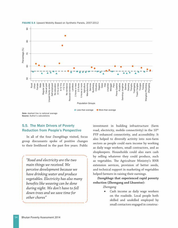
54 Bhutan Poverty Assessment 2014
5.5. the main Drivers of Poverty reduction from People’s Perspective
In all of the four Dzongkhags visited, focus group discussants spoke of positive changes to their livelihood in the past five years. Public
investment in building infrastructure (farm road, electricity, mobile connectivity) in the 10th FYP enhanced connectivity, and accessibility. It also helped to diversify activity into non-farm sectors as people could earn income by working as daily wage workers, small contractors, and as shopkeepers. Households could also earn cash by selling whatever they could produce, such as vegetables. The Agriculture Ministry’s RNR extension services, provision of better seeds, and technical support in marketing of vegetables helped farmers in raising their earnings.
Dzongkhags that experienced rapid poverty reduction (Zhemgang and Lhuentse):
Zhemgang• Cash income as daily wage workers
on the roadside. Local people both skilled and unskilled employed by small contactors engaged in construc-
FIguRE 5.5 Upward Mobility Based on Synthetic Panels, 2007-2012
5060
7080
90
Per
cent
age
(%)
Population Groups
Urb
anR
ural
Fem
ale
Mal
eR
egul
ar p
aid
Cas
ual p
aid
Unp
aid
fam
ily w
orke
rS
elf-e
mpl
oyed
No
educ
atio
n8
Yrs
or l
ess
9-12
Yrs
>12
Yrs
No
rem
itanc
eR
ecei
ved
rem
itanc
eLa
ndle
ss2
Acr
es o
r les
s2-
5 A
cres
5 A
cres
or m
ore
Agr
icul
ture
Man
ufac
turin
gS
ervi
ces
Bum
than
gC
hhuk
haD
agan
aG
asa
Haa
Lhue
ntse
Mon
ggar
Par
oP
ema
Gat
shel
Pun
akha
Sam
drup
Jon
gkha
rS
amts
eS
arpa
ngTh
imph
uTr
ashi
gang
Tras
hi Y
angt
seTr
ongs
aTs
irang
Wan
gdue
Pho
dran
gZh
emga
ng
Less than average More than averageNote: dashed line is national averagesource: Author’s calculations
“Road and electricity are the two main things we received. We perceive development because we have drinking water and produce vegetables. Electricity has also many benefits like weaving can be done during night. We don’t have to fell down trees and we save time for other chores”

55Bhutan Poverty Assessment 2014
tion of houses, building of roads, etc.• Households earned cash income by
selling vegetables in the community, such as to the staff in the gewog and agriculture department RNR centers, and by supplying to boarding schools, teachers, and hospital staff.
• In lower Zhemgang (lower Kheng), oranges are the main cash crop. It was not affected by pests or diseases as badly as in Dagana and Pema Gatshel. The construction of the national highway brought opportunities which greatly increased the market accessibility for orange as well employment opportunities as daily wage workers.
Lhuentse • Accessibility has improved due to
construction of farm roads and other development activities.
Dzongkhags that experienced slow poverty reduction (Dagana and Pema Gatshel):
• Overall improvement in income in the last five years due to developments in infrastructure, farm roads, accessibility to health, education, and RNR extension services.
• Increasing opportunities in the non-farm sectors as wage workers, small contractors, etc.
5.6. Better returns on Individual’s assets underpin Faster reduction in Poverty
The living standard of an individual is a pay-off from participating in the life of society. This pay-off is a function of endowments, behavior and the circumstances that determine the returns on these endowments from any social interaction. Changes in these elements are the result of the structural
transformation that underlies development and ultimately drives distributional change. In particular, Bourguignon, Ferreira and Lustig (2005) identify three key forces that determine observed changes in the distribution of living standards: (i) endowment effects or population effects due to changes in socio-demographic characteristics of the population (e.g., area of residence, age, education, and ownership of physical and financial assets, (ii) price effects due changes in returns on factors of production, and (iii) occupational effects due to changes in the occupational structure of the population.
Given data and other constraints, the focus is on two types of effects: the endowment effect and the effect associated with changes in returns on those endowments. The latter effect is also known as the structural effect. In this reduced-form framework, it is likely that the behavioral effect is mixed up with the price effect. Household per capita expenditure is our living standard indicator, and is a function of both observable and non-observable individual or household characteristics. By applying the Oaxaca-Blinder method20 to decompose the growth incidence curve (GIC) into a component associated with the endowment effect and another related to the structural effect. This decomposition entails running unconditional quintile regressions (Firpo et al., 2009) for the first 99 percentiles of the distribution of log per capita expenditure.
The broad categories of characteristics considered includes: (i) Demographics (e.g., age, marital status, female-headed household, and household size); (ii) Household and community
20 The standard Oaxaca-Blinder decomposition seeks to decompose changes in the unconditional mean outcome into the composition or endowment effect, and the price or structural effects. The method relies on the conditional expectation function (CEF) to summarize the relationship between individual outcomes and individual characteristics, and then on the law of iterated expectations to link the unconditional mean to characteristics. Fortin et al. (2011) have extended this logic to the decomposition of changes in other distributional statistics beyond the unconditional mean, such as quantiles.

56 Bhutan Poverty Assessment 2014
assets (e.g., years of education, durable goods, such as fridge, electric iron, TV, etc., land ownership, ownership of livestock, distance to nearest agricultural extension service center, distance to nearest hospital, distance to nearest tarred road, distance to nearest feeder road, distance to dzongkhag headquarters, and distance to nearest bank); (iii) Sector of employment (e.g., primary, secondary, non-public services, public sector, non-paid labour); and (iv) Area/dzongkhag of residence.21 Durables are included among the characteristics because they are excluded from consumption expenditure (see RGoB, 2013).
We therefore use the analogy between growth accounting and the counterfactual decomposition of the GIC considered to link the endowment effect to notion of accumulation (of factors of production) and we take the structural effect to be an indicator of productivity in socioeconomic interaction. Accumulation and productivity are indeed the two basic ideas that structure the study of economic growth.
5.7. Composition versus structure
Figure 5.6 shows a decomposition of the total variation in the distribution of log per capita expenditure (essentially the GIC) into two components. The first component is due to changes in the distribution of characteristics while the second represents the contribution of changes in the distribution of returns to those characteristics.
The structural effect is roughly U-shaped. The fact that it is downward sloping up to the 77th percentile means that the structural effect reduces inequality in that part of the distribution and tends to increase it in the upper segment
21 Our choice of dummy variables implies that the reference case (conditional on characteristics represented by continuous variables) is landless, does not own any of the durables listed in the equation, resides in Thimphu in a male-headed household, and the sector of employment is listed as other.
of the distribution. The endowment effect has roughly an inverted U-shape. It is upward sloping up to the 77th percentile and therefore increases inequality over much of the distribution. The structural effect dominates the endowment effect at the low end of the distribution up to the 28th percentile. It turns negative between the 60th and 95th percentile. The endowment effect is mostly positive and overwhelms the structural effect past the 28th percentile. The configuration of the three curves presented in Figure 5.6 implies that the level of the GIC is determined mainly by the composition or endowment effect. In particular, the gains achieved by people located at the bottom of the distribution up to the 28th percentile are due to the structural effect while the gains beyond that point are due mainly to
FIguRE 5.6 A Decomposition of Growth Incidence in Bhutan, 2007-2012
-20
-10
0
10
20
30
40
0 10 20 30 40 50 60 70 80 90 100Expenditure Percentiles
Overall Incidence
Endowment Effect
Structural Effect
Ann
ual G
row
th R
ate
(%)
source: Author’s calculations
“The opening of school has overall benefitted the community. Previously we have to send our children to school which were far off. Sending children far off places adds to additional expenditure on travel, living arrangement cost”
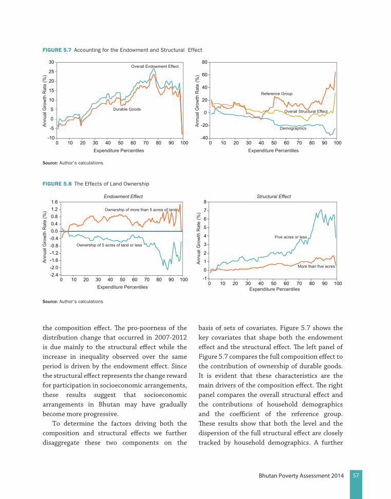
57Bhutan Poverty Assessment 2014
the composition effect. The pro-poorness of the distribution change that occurred in 2007-2012 is due mainly to the structural effect while the increase in inequality observed over the same period is driven by the endowment effect. Since the structural effect represents the change reward for participation in socioeconomic arrangements, these results suggest that socioeconomic arrangements in Bhutan may have gradually become more progressive.
To determine the factors driving both the composition and structural effects we further disaggregate these two components on the
basis of sets of covariates. Figure 5.7 shows the key covariates that shape both the endowment effect and the structural effect. The left panel of Figure 5.7 compares the full composition effect to the contribution of ownership of durable goods. It is evident that these characteristics are the main drivers of the composition effect. The right panel compares the overall structural effect and the contributions of household demographics and the coefficient of the reference group. These results show that both the level and the dispersion of the full structural effect are closely tracked by household demographics. A further
FIguRE 5.7 Accounting for the Endowment and Structural Effect
-10
-5
0
5
10
15
20
25
30
0 10 20 30 40 50 60 70 80 90 100
Durable Goods
Overall Endowment Effect
Overall Structural Effect
Reference Group
DemographicsAnn
ual G
row
th R
ate
(%)
Ann
ual G
row
th R
ate
(%)
-40
-20
0
20
40
60
80
0 10 20 30 40 50 60 70 80 90 100
source: Author’s calculations
FIguRE 5.8 The Effects of Land Ownership
-2.4-2.0-1.6-1.2-0.8-0.40.00.40.81.21.6
0 10 20 30 40 50 60 70 80 90 100Expenditure Percentiles Expenditure Percentiles
Endowment Effect Structural Effect
Ownership of 5 acres of land or less
More than five acres
Ownership of more than 5 acres of land
Five acres or less
Ann
ual G
row
th R
ate
(%)
Ann
ual G
row
th R
ate
(%)
-1
0
1
2
3
4
5
6
7
8
0 10 20 30 40 50 60 70 80 90 100
source: Author’s calculations
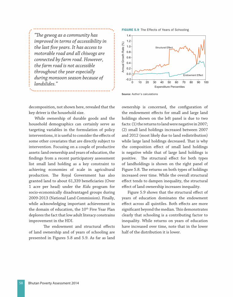
58 Bhutan Poverty Assessment 2014
decomposition, not shown here, revealed that the key driver is the household size.
While ownership of durable goods and the household demographics can certainly serve as targeting variables in the formulation of policy interventions, it is useful to consider the effects of some other covariates that are directly subject to intervention. Focusing on a couple of productive assets: land ownership and years of education, the findings from a recent participatory assessment list small land holding as a key constraint to achieving economies of scale in agricultural production. The Royal Government has also granted land to about 61,339 beneficiaries (Over 1 acre per head) under the Kidu program for socio-economically disadvantaged groups during 2009-2013 (National Land Commission). Finally, while acknowledging important achievement in the domain of education, the 10th Five Year Plan deplores the fact that low adult literacy constrains improvement in the HDI.
The endowment and structural effects of land ownership and of years of schooling are presented in Figures 5.8 and 5.9. As far as land
ownership is concerned, the configuration of the endowment effects for small and large land holdings shown on the left panel is due to two facts: (1) the returns to land were negative in 2007; (2) small land holdings increased between 2007 and 2012 (most likely due to land redistribution) while large land holdings decreased. That is why the composition effect of small land holdings is negative while that of large land holdings is positive. The structural effect for both types of landholdings is shown on the right panel of Figure 5.8. The returns on both types of holdings increased over time. While the overall structural effect tends to dampen inequality, the structural effect of land ownership increases inequality.
Figure 5.9 shows that the structural effect of years of education dominates the endowment effect across all quintiles. Both effects are more significant beyond the median. This demonstrates clearly that schooling is a contributing factor to inequality. While returns on years of education have increased over time, note that in the lower half of the distribution it is lower.
“The gewog as a community has improved in terms of accessibility in the last five years. It has access to motorable road and all chiwogs are connected by farm road. However, the farm road is not accessible throughout the year especially during monsoon season because of landslides.”
FIguRE 5.9 The Effects of Years of Schooling
-0.2
0.0
0.2
0.4
0.6
0.8
1.0
1.2
1.4
0 10 20 30 40 50 60 70 80 90 100Expenditure Percentiles
Structural Effect
Endowment Effect
Ann
ual G
row
th R
ate
(%)
source: Author’s calculations
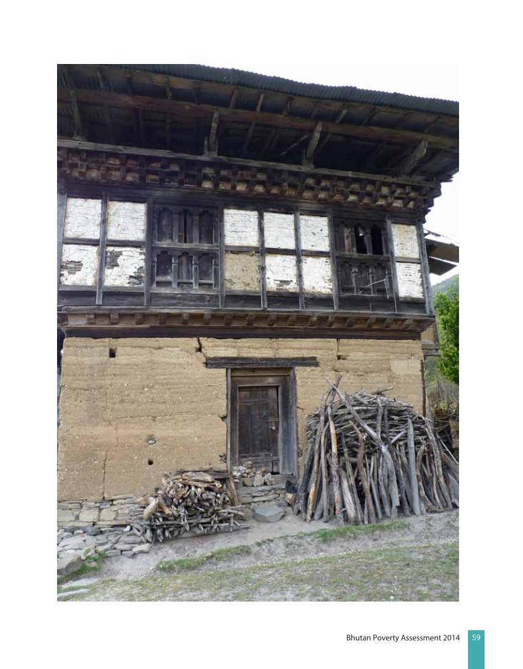
59Bhutan Poverty Assessment 2014
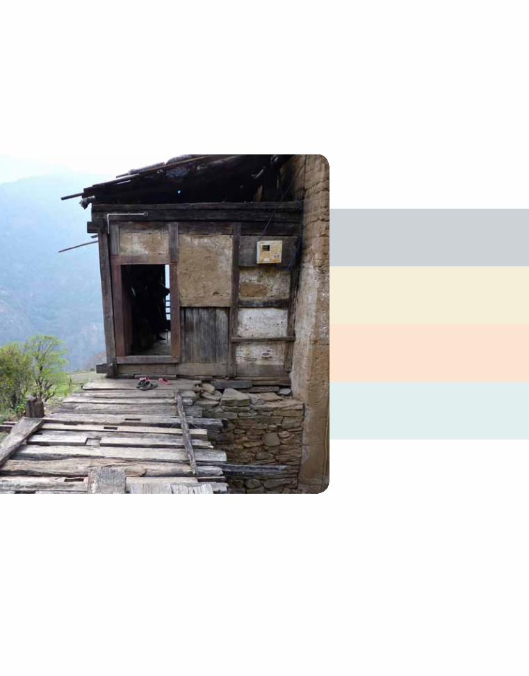

61Bhutan Poverty Assessment 2014
Poverty Reduction in Bhutan: Sustainability, Vulnerability and Suggested Remediation
The current pace of poverty reduction appears sustainable in the medium term. The policy foundations of the current poverty reduction achievement lie in trade intensification with neighbors, rural infrastructure expansion, and development impetus from hydroelectric power. At the household level, the emphasis on education of children seen across all economic classes is a welcome sign that families will be able to seek out these opportunities to escape poverty.
Trade intensification with neighbors is set to continue. The existing, 10-year free trade agreement with India is due for renewal in 2016, and this is likely to be concluded. The bilateral agreement with Bangladesh, which has benefited Bhutan by preferential duty free access to 74 mostly agricultural exports, is due for renewal in 2018. In addition, bilateral agreements with Thailand and Nepal are also on the anvil. Under the South Asian Free Trade Agreement, Bangladesh is grouped with Bhutan as “least developed members” with slower pace of tariff reduction to 0-5 percent by 2016, and this could erode the 15 percent preference margin currently enjoyed by Bhutan in orange and apple exports to Bangladesh. However, Bhutan is a net exporter of
these fruits in the north-east region of the Indian sub-continent and the trade logistical gains made by then should be able to sustain fruit exports to Bangladesh. In addition, tariff reduction under SAFTA is scheduled on a graduated annual basis over eight years. India’s north-east region (Arunachal Pradesh, Assam, Manipur, Meghalaya, Mizoram, Nagaland, and Tripura) with an agro-climate similar to Bhutan’s is likely to become a potential competitor in horticultural products. But growth dynamism in India and Bangladesh should be able to accommodate expansion of differentiated products from Bhutan.
The infrastructure within and beyond Bhutan is set for significant improvement. The 20-year road sector master plan for Bhutan, 2007-2027, has a prioritized plan for expansion of improving inter-Dzongkhag connectivity (feeder roads, highways) and the completion of the Southern East-West Highway. An additional 2,654 km of feeder roads (connecting gewogs to dzongkhag headquarters), 537 km of inter-dzongkhag highways, including tunnels, and 794 km of Southern East-West highway are planned to be completed. These developments in conjunction with the 4,000 km expansion, “from the bottom up”– farm roads first –during the 10th
6Chapter
62 Bhutan Poverty Assessment 2014
FYP, if built according to plan, have the potential to greatly improve long-term welfare of especially rural households. The international competitive advantage of Bhutan will be enhanced by the completion of the Southern East-West Highway that runs parallel to the Indian border. Bhutan could benefit from the development of a road corridor connecting South Asia with South-East Asia through Myanmar under the Bay of Bengal
Initiative for Multi-Sectoral Technical and Economic Cooperation (BIMSTEC). There are as many initiatives to develop infrastructure as there are regional cooperation agreements.
Expansion of hydroelectric power in Bhutan through 2020 will aid poverty reduction both directly and indirectly. Bhutan’s plans to increase six-fold its current capacity for electric power to 10 GW by 2020, with India as the main
“The income from the oranges has gone down from average Nu 50,000 to Nu 20,000 so we do not know what to do next. May be we should plant mountain hazelnut as an alternative. Heard that a weather condition of our area is similar to that of Lingmithang in Monggar and it might work here” – A male FGD participant, Shumar, Pema Gatshel
“Many orange orchards are damaged by disease these days. Now oranges are not even available to eat. First it affected the trees in Denchi village and shifted upwards. Many people of our locality believe that dust from Gypsum powder factory leads to dying of the crops as well as orange” – A female FGD participant, Shumar, Pema Gatshel
“I didn’t see the insect but the root of the orange tree has been damaged”– A female FGD participant, Shumar, Pema Gatshel.
“According to the agriculture sector the solution to the disease is after many rounds of discussion we have been advised to cut down all the orange trees even if all the trees in the orchard are not affected. If even one tree is affected rest of the trees also have to be cut down and burnt. The government is providing free orange saplings. Now farmers are apprehensive to the advice because the question is how they would manage without income until the new trees start bearing fruits. It takes at least five years to start bearing fruits” – A key informant, Shumar, Pema Gatshel
“Because of water scarcity we depend on monsoon rain to transplant paddy. When there is monsoon everyone in the village start transplanting paddy and therefore we cannot exchange labour and sometimes we have to keep our land fallow” – A male participant, Nangkhor community, Zhemgang
63Bhutan Poverty Assessment 2014
export market. Big projects under construction (Punatsangchhu I and II, Mangdechhu, and Dagachhu) will add 3 GW of capacity to the current capacity of 1.6 GW, reaching half-way to the goal of 10 GW by 2017. If more new plant agreements are signed and implemented from now until 2020, they will continue to give development impetus during the construction and the generation phases.
The current trend toward commercial crop production carries common risks. With limited land, increasing fragmentation of land holdings (“as children get married they demand their own land”), and rural to urban migration of working age adults, labour-intensive horticulture will become difficult. Contract farming by large-scale land owners may be a way to sustain exports but benefits to poorer farmers might diminish. The current problems faced by farmers, such as the incurable “greening disease” of oranges, diseases of the cardamom plants, and regular raids into farms by elephants (in low land), monkeys, and wild boars have been difficult to solve. The alternative of planting disease-resistant plants is a running battle. The option of genetically modified plants is also against the organic farming trend. It takes years to bring horticultural crops to harvest and equally long to shift to other profitable production. Some farmers (mainly the rich) have shifted to walnuts, but these, too, take many years to harvest.
Besides risks at societal level, some population groups face a variety of challenges. Bhutanese can take justifiable pride in community support for individual families. BLSS 2012 social capital module analysis showed that 70 percent of rural households and 60 percent of urban households had five or more individuals to turn to for support in case of emergencies. Despite this mutual support, for every 10 families that moved out of poverty two were falling into poverty. While the churning around the poverty line is less pervasive in Bhutan than in many other countries, reliance on community support is not proving adequate for some. Bhutan has no formal social protection mechanisms to help individuals ride out of hard times. Risk of downward mobility is greater than average (Figure 6.4) for rural residents, male-headed households, people in informal jobs (casual and self-employed), those with low education levels, and particularly high for those living in poorer dzongkhags (Pema Gatshel, Dagana, Samtse, Trashigang, and Tsirang).
Female-headed households have pointed out in focus group discussions that no one was willing to participate with them in labour exchange arrangements at times of peak farm labour needs.
The suggested remedial measures for adverse shocks are formal social protection programs for individuals. At present, individuals cope with shocks mostly by drawing on own savings if they are non-poor, and by borrowing from friends,
“One of the main problems is that we are not able to protect our crop from wild animals such as wild boars and monkeys. On top of that important cash crops like oranges and cardamom have been affected by diseases and their yield have declined over the years. These problems have also resulted some of the households to migrate to urban areas. When one household migrates other households also tend to migrate thus turning farms into thick jungle making it easier for wild animals to attack crops in the locality” – A male FGD participant, Kana Community, Dagana
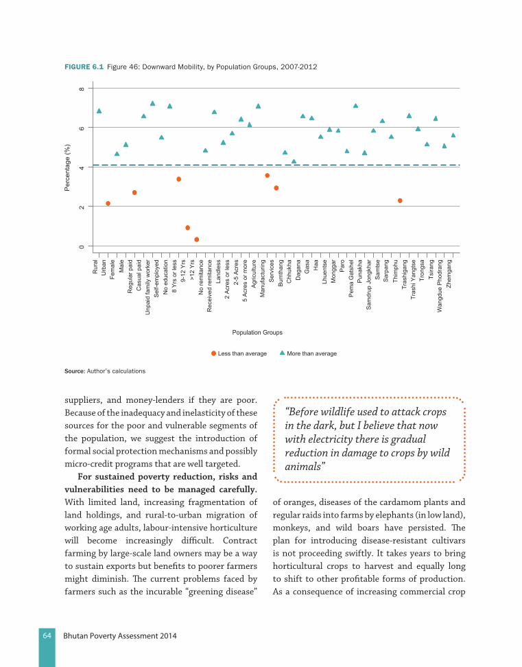
64 Bhutan Poverty Assessment 2014
suppliers, and money-lenders if they are poor. Because of the inadequacy and inelasticity of these sources for the poor and vulnerable segments of the population, we suggest the introduction of formal social protection mechanisms and possibly micro-credit programs that are well targeted.
For sustained poverty reduction, risks and vulnerabilities need to be managed carefully. With limited land, increasing fragmentation of land holdings, and rural-to-urban migration of working age adults, labour-intensive horticulture will become increasingly difficult. Contract farming by large-scale land owners may be a way to sustain exports but benefits to poorer farmers might diminish. The current problems faced by farmers such as the incurable “greening disease”
of oranges, diseases of the cardamom plants and regular raids into farms by elephants (in low land), monkeys, and wild boars have persisted. The plan for introducing disease-resistant cultivars is not proceeding swiftly. It takes years to bring horticultural crops to harvest and equally long to shift to other profitable forms of production. As a consequence of increasing commercial crop
FIguRE 6.1 Figure 46: Downward Mobility, by Population Groups, 2007-2012
Urb
anR
ural
Fem
ale
Mal
eR
egul
ar p
aid
Cas
ual p
aid
Unp
aid
fam
ily w
orke
rS
elf-e
mpl
oyed
No
educ
atio
n8
Yrs
or l
ess
9-12
Yrs
>12
Yrs
No
rem
itanc
eR
ecei
ved
rem
itanc
eLa
ndle
ss2
Acr
es o
r les
s2-
5 A
cres
5 A
cres
or m
ore
Agr
icul
ture
Man
ufac
turin
gS
ervi
ces
Bum
than
gC
hhuk
haD
agan
aG
asa
Haa
Lhue
ntse
Mon
ggar
Par
oP
ema
Gat
shel
Pun
akha
Sam
drup
Jon
gkha
rS
amts
eS
arpa
ngTh
imph
uTr
ashi
gang
Tras
hi Y
angt
seTr
ongs
aTs
irang
Wan
gdue
Pho
dran
gZh
emga
ng
02
46
8
Per
cent
age
(%)
Population Groups
Less than average More than average
source: Author’s calculations
“Before wildlife used to attack crops in the dark, but I believe that now with electricity there is gradual reduction in damage to crops by wild animals”
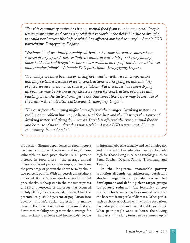
65Bhutan Poverty Assessment 2014
production, Bhutan dependence on food imports has been rising over the years, making it more vulnerable to food price shocks. A 12 percent increase in food prices – the average annual increase in recent years - for example, can increase the percentage of poor in the short-term by about two percent points. With all petroleum products imported, Bhutan’s poor also face risk from fuel price shocks. A sharp rise in the consumer prices of LPG and kerosene of the order that occurred in July 2013 (quickly reversed, however) had the potential to push 0.5 percent of population into poverty. Bhutan’s social protection is mainly through the Royal Kidu welfare program. Risks of downward mobility are greater than average for rural residents, male-headed households, people
in informal jobs (the casually and self-employed), and those with low education and particularly high for those living in select dzongkhags such as Pema Gatshel, Dagana, Samtse, Trashigang, and Tsirang).
In the long-term, sustainable poverty reduction depends on addressing persistent shocks, engendering private sector led development and defining clear target groups for poverty reduction. The feasibility of crop insurance for farmers may be examined to protect the harvests from perils of diseases. Other perils, such as those associated with wild-life predation, have also persisted and evaded viable solutions. What poor people want to better their living standards in the long term can be summed up as
“For this community maize has been principal food from time immemorial. People use to grow maize and eat as a special diet to work in the fields but due to drought we could not harvest like before which has affected our food security” – A male FGD participant, Drujeygang, Dagana
“We have lot of wet land for paddy cultivation but now the water sources have started drying up and there is limited volume of water left for sharing among households. Lack of irrigation channel is a problem on top of that due to which wet land remains fallow” – A female FGD participant, Drujeygang, Dagana
“Nowadays we have been experiencing hot weather with rise in temperature and may be this is because of lot of constructions works going on and building of factories elsewhere which causes pollution. Water sources have been drying up because may be we are using excessive wood for construction of houses and blasting. Even the taste of oranges is not that sweet like before may be because of the heat” – A female FGD participant, Drujeygang, Dagana
“The dust from the mining might have affected the oranges. Drinking water was really not a problem but may be because of the dust and the blastings the source of drinking water is shifting downwards. Dust has affected the trees, animal fodder and because of no rain dust does not settle” – A male FGD participant, Shumar community, Pema Gatshel
66 Bhutan Poverty Assessment 2014
access to roads, electricity, public transportation, irrigation, land and higher education. Sustained poverty reduction depends on job opportunities and wage earnings of the poor. The development paradigm for a renewable resource rich country like Bhutan would call for engendering private sector led growth actively enabled by the public sector. Successful agribusiness – an emerging sector in Bhutan - will require development of value chain system (from farm to market) that will identify and remove the bottlenecks that farmers encounter including constraints related to finance and availability of crop insurance. The
government could engender private investment in hydropower sector by Private Public Partnerships and subcontracting in order to create jobs. The Royal Government of Bhutan seems to favor complementary use of consumption and multidimensional poverty. But the overlap of the two approaches identifying the poor is small. Therefore defining a clear target group for poverty reduction is important. Also, with success in reducing extreme consumption poverty rapidly, the goal could be now shift to shared prosperity defined for example as he welfare of the bottom 40 percent of the population.
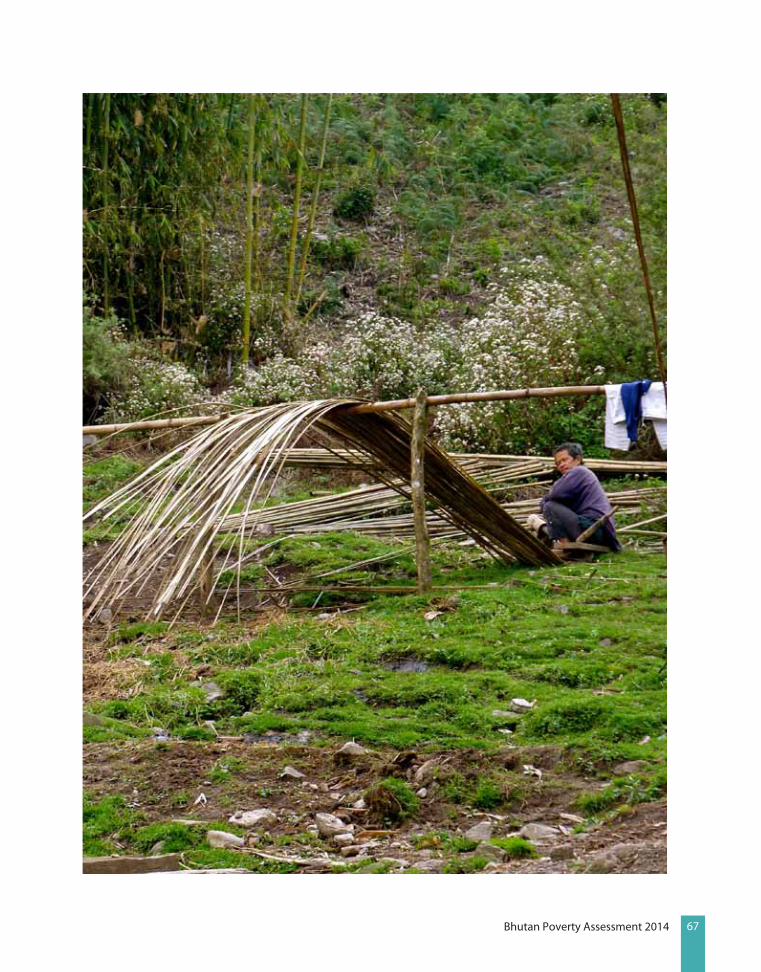
67Bhutan Poverty Assessment 2014

Annex A: sources of variation in Poverty outcomes in Bhutan
abstract
This annex uses data from the 2007 and 2012 rounds of the BLSS to assess the poverty outcomes associated with the implementation of the 10th Five Year Plan (2008-2013). During the period under consideration, poverty incidence in Bhutan fell significantly, from about 23 percent in 2007 to about 12 percent in 2012. Inequality remained almost constant with the Gini coefficient hovering around 38 percent. It is clear that this impressive reduction in poverty is due mainly to growth in per-capita expenditure. A decomposition of the
growth incidence curve (GIC) reveals that the growth process was clearly pro-poor in the sense that socioeconomic institutions rewarded the poor more than the non-poor. Furthermore, a decomposition of the urban-rural differential also shows that the reduction in urban bias is due mainly to the fact that the growth process favors the rural sector relative to the urban. Overall, these findings suggest that socioeconomic arrangements in Bhutan have become more progressive over time.

69Bhutan Poverty Assessment 2014
Introduction
The RGoB has made the pursuit of national happiness the overarching goal of its development strategy. In that context, it is committed to improving the quality of life for the citizens through inclusive and sustainable economic growth, the conservation of the natural environment, the preservation of the country’s cultural heritage and good governance. These focal areas constitute the four pillars spanning the concept of GNH, and are being implemented through a series of five year plans. The vision underlying this strategic framework has been enshrined in the 2008 Constitution adopted at the beginning of the 10th Five Year Plan.
The RGoB has made poverty reduction the central theme and main objective of the 10th Plan. It is pursuing this objective through industrial development, national spatial planning, integrated rural-urban development, strategic expansion of infrastructure, human capital development, and enhancement of the enabling environment. The formulation of the 10th Plan builds on the strong achievements of the Ninth Plan (2002-1007) which sought to improve the quality of life and income, with a special focus on the poor, by promoting good governance and private sector-driven economic growth in addition to preserving cultural heritage and the natural environment.
During the Ninth Plan, real GDP grew on average by 9.6 percent between 2003 and 2007, increasing real GDP from Nu 23.5 billion in 2002 to Nu 37.5 billion in 2007. This impressive growth, driven mainly by a continuous and sustained expansion of the electricity sector, caused the GDP per capita to reach its highest level ever recorded, estimated at US$1,414 in 2006 compared to US$835 in 2002 (IMF, 2010a). In terms of sectoral growth performance, available information suggests that the primary sector (agriculture, livestock, and forestry) grew
the least, at an estimated average of 1.3 percent, about one-half of the target rate. Trade and other services performed better, achieving an average growth rate of 13 percent, higher than the target rate.
The process of economic growth led to significant changes in the composition of GDP. During the Ninth Plan, the share of the primary sector fell from 29 percent to 20.3 percent. By the end of that Plan, the secondary and tertiary sectors accounted for 43 percent and 36 percent of GDP respectively. The importance of the secondary sector is linked mainly to growth in electricity and construction; it does not reflect any significant developments in manufacturing (IMF, 2010a).
A Joint World Bank-IMF staff advisory note assessing the 2009 Poverty Reduction Strategy (IMF, 2010b) notes that the strong performance of the economy under the Ninth Plan, along with improvements in governance, have put Bhutan firmly on track to achieve most of the Millennium Development Goals (MDGs). Poverty incidence fell from 36 percent in 2000 to about 23 percent in 2007. The Gross Primary Enrolment Rate (GPER) in schools increased from 81 percent in 2002 to 109 percent in 2007. The country has achieved gender parity in both primary and basic education due to the fact that the enrolment rate was growing faster for girls than for boys at the primary and secondary levels of education. During the same plan period, sustained investments in both human resources and physical capital in the health sector led to significant improvement in the health status of the population. Under-five mortality dropped significantly from 84 per thousand to 60 per thousand live births. Maternal mortality decreased from 255 to about 215 per hundred thousand live births. Access to safe drinking water and sanitation expanded considerably under the Ninth Plan.
70 Bhutan Poverty Assessment 2014
The socioeconomic improvements brought about by the plan implementation are reflected also in changes in the Human Development Index (HDI), which combines three indicators of aggregate living standard: (i) life expectancy, (ii) educational achievement, and (iii) GDP per capita. The HDI has almost doubled in value over the past 20 years or so. By 2006, Bhutan ranked 131st among all countries surveyed. In the 1980s, improvements in the HDI were due mostly to increases in life expectancy and real per capita GDP. During the Ninth Plan, life expectancy stagnated at around 66 years so that improvements in the HDI observed over that period were due mostly to increases in enrolment rates in primary and secondary education, and in GPD per capita (IMF, 2010a).
The purpose of this annex is to provide an account of the poverty outcomes observed under the 10th Plan, which serves also as the RGoB’s Poverty Reduction Strategy Paper (PRSP). This account is based on data from the 2007 and 2012 rounds of the BLSS. Given the period of this plan, the 2007 data provide a valid baseline for an assessment of the poverty outcomes of this plan. Similarly the 2012 data are considered endline observations, reflecting the outcome of the implementation of the 10th Plan although the plan formally ended in 2013.
Policy analysis can be considered a process designed to produce evidence to answer important questions that policymakers and other key stakeholders might have about design, performance, or results. In the context of evidence-based decision-making, policymakers are interested in what works and why. There is evidence that poverty reduction under the 10th Plan has been as impressive as under the preceding plan. In particular, poverty incidence (based on household per capita expenditure) fell again significantly from about 23 percent in 2007 to 12 percent in 2012. All other poverty measures
considered also indicate rapid poverty reduction. The key question addressed in this paper therefore is: What drives this impressive poverty reduction? A reliable answer to this question might shed some light on why some areas or socioeconomic groups lag behind despite this strong aggregate performance.
The importance of the key question above stems from the fact that an aggregate judgment about changes in poverty outcomes may hide more than it reveals about the heterogeneity of impacts underpinning the aggregate outcome. Yet a deeper understanding of this diversity of impact is required if one is to better calibrate interventions for poverty reduction. Resource-allocation mechanisms adopted in the 10th Plan thus strive to account for the poverty status of the potential beneficiaries, among other considerations.
The credibility and hence the usefulness of an answer to a policy question hinges critically on the quality of its informational basis, consist-ing of available facts (data) and the logic used to analyze and interpret those facts. The approach followed in this paper is motivated by the fol-lowing considerations. Poverty measures and all other distributional statistics are computed on the basis of a distribution of living standards across individuals or households. This observa-tion implies that changes in poverty outcomes reflect variations in the underlying distribution of individual outcomes. Thus, a distributional change is pro-poor if it involves poverty reduc-tion for some choice of poverty index. Given that a distribution is fully characterized by its mean and the degree of inequality, several authors (e.g., Datt and Ravallion, 1992) have proposed counterfactual decomposition meth-ods to identify the contribution of changes in the mean and in inequality to variations in overall poverty. Within this framework, the contribution of a change in the mean is known

71Bhutan Poverty Assessment 2014
as the size effect while the effect of a change in relative inequality is the redistribution effect (Essama-Nssah, 2012).
The usefulness of the size and redistribution effects in policymaking is severely limited by the fact that these effects account for changes in poverty on the basis of variation in summary statistics that are hard to target with policy instruments. Therefore, there is a need to link observed poverty outcomes to factors associated with deep structural elements that drive individual behavior and social interaction. The living standard of an individual is a pay-off from her participation in the life of society. This pay-off is a function of endowments, behavior, and the circumstances that determine the returns on these endowments from any social interaction. Changes in these elements are the result of the structural transformation that underlies development and ultimately drives distributional change. In particular, Bourguignon, Ferreira, and Lustig (2005) identify three key forces that determine observed changes in the distribution of living standards: (i) endowment effects or population effects due to changes in socio-demographic characteristics of the population (e.g., area of residence, age, education, and ownership of physical and financial assets, (ii) price effects (also known as structural effects) due to changes in returns on factors of production, and (iii) occupational effects due to changes in the occupational structure of the population.
Given data and other constraints, this paper focuses only on two types of effects: (i) the endowment effect and (ii) the structural effect associated with changes in returns on those endowments. In this reduced-form framework, it is likely that the behavioral effect is mixed up with the price effect. Household per capita expenditure is our living standard indicator, and is a function of both observable and non-observable individual or household characteristics. It is possible to decompose directly changes in poverty into the
endowment and structural effects. However, we find it more informative to conduct the analysis in terms distributional change driving the variation in poverty outcomes. This approach is supported by the fact that, for the class of additively separable poverty measure, which includes FGT measures and the Watts index, a change in poverty over time can be written as a weighted sum of points along the growth incidence curve (GIC) up to the poverty line (Essama-Nssah and Lambert, 2009). Basically, we apply the Oaxaca-Blinder method1 to decompose the GIC into a component associated with the endowment effect and another related to the structural effect. This decomposition entails running unconditional quantile regressions (Firpo et al., 2009) for the first 99 percentiles of the distribution of log per capita expenditure.
The rest of this annex is organized as follows: Section 1 describes the observed outcomes in poverty, growth, and inequality, and confirms that the implementation of the 10th Plan led to an impressive poverty reduction; Section 2 focuses on the endowment and structural effects associated with distributional changes over time and across areas of residence, particularly the urban-rural differential (the available data could not support the same type of analysis at dzongkhag level); and Section 3 carries concluding remarks. The annex concludes with a set of Data Tables.
1. underlying Distributional Change and associated Poverty outcomes
A fundamental step in answering the key question raised in the introduction to this paper entails describing what happened to consumption
1 The standard Oaxaca-Blinder decomposition seeks to decompose changes in the unconditional mean outcome the composition or endowment effect and the price or structural effect. The method relies on the conditional expectation function (CEF) to summarize the relationship between individual outcomes and individual characteristics, and then on the law of iterated expectations to link the unconditional mean to characteristics. Fortin et al. (2011) have extended this logic to the decomposition of changes in other distributional statistics beyond the unconditional mean, such as quantiles.
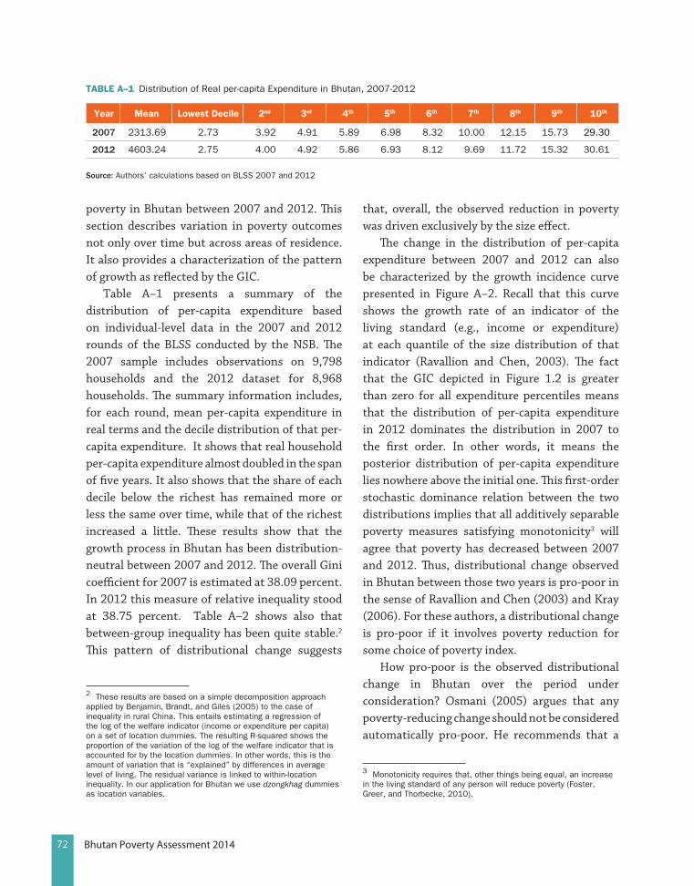
72 Bhutan Poverty Assessment 2014
poverty in Bhutan between 2007 and 2012. This section describes variation in poverty outcomes not only over time but across areas of residence. It also provides a characterization of the pattern of growth as reflected by the GIC.
Table A–1 presents a summary of the distribution of per-capita expenditure based on individual-level data in the 2007 and 2012 rounds of the BLSS conducted by the NSB. The 2007 sample includes observations on 9,798 households and the 2012 dataset for 8,968 households. The summary information includes, for each round, mean per-capita expenditure in real terms and the decile distribution of that per-capita expenditure. It shows that real household per-capita expenditure almost doubled in the span of five years. It also shows that the share of each decile below the richest has remained more or less the same over time, while that of the richest increased a little. These results show that the growth process in Bhutan has been distribution-neutral between 2007 and 2012. The overall Gini coefficient for 2007 is estimated at 38.09 percent. In 2012 this measure of relative inequality stood at 38.75 percent. Table A–2 shows also that between-group inequality has been quite stable.2 This pattern of distributional change suggests
2 These results are based on a simple decomposition approach applied by Benjamin, Brandt, and Giles (2005) to the case of inequality in rural China. This entails estimating a regression of the log of the welfare indicator (income or expenditure per capita) on a set of location dummies. The resulting R-squared shows the proportion of the variation of the log of the welfare indicator that is accounted for by the location dummies. In other words, this is the amount of variation that is “explained” by differences in average level of living. The residual variance is linked to within-location inequality. In our application for Bhutan we use dzongkhag dummies as location variables.
that, overall, the observed reduction in poverty was driven exclusively by the size effect.
The change in the distribution of per-capita expenditure between 2007 and 2012 can also be characterized by the growth incidence curve presented in Figure A–2. Recall that this curve shows the growth rate of an indicator of the living standard (e.g., income or expenditure) at each quantile of the size distribution of that indicator (Ravallion and Chen, 2003). The fact that the GIC depicted in Figure 1.2 is greater than zero for all expenditure percentiles means that the distribution of per-capita expenditure in 2012 dominates the distribution in 2007 to the first order. In other words, it means the posterior distribution of per-capita expenditure lies nowhere above the initial one. This first-order stochastic dominance relation between the two distributions implies that all additively separable poverty measures satisfying monotonicity3 will agree that poverty has decreased between 2007 and 2012. Thus, distributional change observed in Bhutan between those two years is pro-poor in the sense of Ravallion and Chen (2003) and Kray (2006). For these authors, a distributional change is pro-poor if it involves poverty reduction for some choice of poverty index.
How pro-poor is the observed distributional change in Bhutan over the period under consideration? Osmani (2005) argues that any poverty-reducing change should not be considered automatically pro-poor. He recommends that a
3 Monotonicity requires that, other things being equal, an increase in the living standard of any person will reduce poverty (Foster, Greer, and Thorbecke, 2010).
TABlE A–1 Distribution of Real per-capita Expenditure in Bhutan, 2007-2012
Year Mean lowest Decile 2nd 3rd 4th 5th 6th 7th 8th 9th 10th
2007 2313.69 2.73 3.92 4.91 5.89 6.98 8.32 10.00 12.15 15.73 29.30
2012 4603.24 2.75 4.00 4.92 5.86 6.93 8.12 9.69 11.72 15.32 30.61
source: Authors’ calculations based on BLSS 2007 and 2012
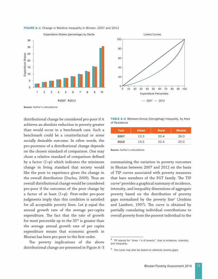
73Bhutan Poverty Assessment 2014
distributional change be considered pro-poor if it achieves an absolute reduction in poverty greater than would occur in a benchmark case. Such a benchmark could be a counterfactual or some socially desirable outcome. In other words, the pro-poorness of a distributional change depends on the chosen standard of comparison. One may chose a relative standard of comparison defined by a factor (1+ρ) which indicates the minimum change in living standard that society would like the poor to experience given the change in the overall distribution (Duclos, 2009). Thus an overall distributional change would be considered pro-poor if the outcomes of the poor change by a factor of at least (1+ρ). First-order pro-poor judgments imply that this condition is satisfied for all acceptable poverty lines. Let ρ equal the annual growth rate of the average per-capita expenditure. The fact that the rate of growth for most percentile up to the 35th is greater than the average annual growth rate of per capita expenditure means that economic growth in Bhutan has been pro-poor to the first-order.
The poverty implications of the above distributional change are presented in Figure A–3
summarizing the variation in poverty outcomes in Bhutan between 2007 and 2012 on the basis of TIP curves associated with poverty measures that bare members of the FGT family. The TIP curve4 provides a graphical summary of incidence, intensity, and inequality dimensions of aggregate poverty based on the distribution of poverty gaps normalized by the poverty line5 (Jenkins and Lambert, 1997). The curve is obtained by partially cumulating individual contributions to overall poverty from the poorest individual to the
4 TIP stands for “three ‘i’s of poverty”, that is incidence, intensity, and inequality.
5 The curve may also be based on absolute poverty gaps.
FIguRE A–1 Change in Relative Inequality in Bhutan, 2007 and 2012
00
20
40
60
80
100
10 20 30 40 50 60 70 80 90 100
Expenditure Percentiles
Lorenz CurvesExpenditure Shares (percentage) by Decile
2007 2012
0
5
10
15
20
25
30
35
1 2 3 4 5 6 7 8 9 10
2007 2012
Exp
endi
ture
Sha
res
source: Author’s calculations
TABlE A–2 Between-Group (Dzongkhag) Inequality, by Area of Residence
Year urban Rural Bhutan
2007 13.3 20.4 26.0
2012 14.5 22.4 25.0
source: Author’s calculations
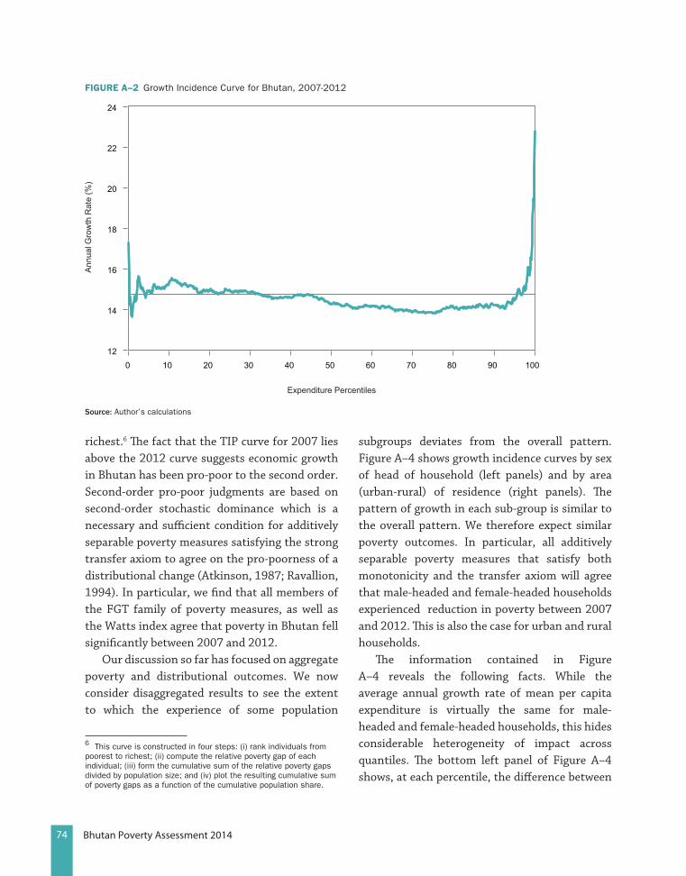
74 Bhutan Poverty Assessment 2014
richest.6 The fact that the TIP curve for 2007 lies above the 2012 curve suggests economic growth in Bhutan has been pro-poor to the second order. Second-order pro-poor judgments are based on second-order stochastic dominance which is a necessary and sufficient condition for additively separable poverty measures satisfying the strong transfer axiom to agree on the pro-poorness of a distributional change (Atkinson, 1987; Ravallion, 1994). In particular, we find that all members of the FGT family of poverty measures, as well as the Watts index agree that poverty in Bhutan fell significantly between 2007 and 2012.
Our discussion so far has focused on aggregate poverty and distributional outcomes. We now consider disaggregated results to see the extent to which the experience of some population
6 This curve is constructed in four steps: (i) rank individuals from poorest to richest; (ii) compute the relative poverty gap of each individual; (iii) form the cumulative sum of the relative poverty gaps divided by population size; and (iv) plot the resulting cumulative sum of poverty gaps as a function of the cumulative population share.
subgroups deviates from the overall pattern. Figure A–4 shows growth incidence curves by sex of head of household (left panels) and by area (urban-rural) of residence (right panels). The pattern of growth in each sub-group is similar to the overall pattern. We therefore expect similar poverty outcomes. In particular, all additively separable poverty measures that satisfy both monotonicity and the transfer axiom will agree that male-headed and female-headed households experienced reduction in poverty between 2007 and 2012. This is also the case for urban and rural households.
The information contained in Figure A–4 reveals the following facts. While the average annual growth rate of mean per capita expenditure is virtually the same for male-headed and female-headed households, this hides considerable heterogeneity of impact across quantiles. The bottom left panel of Figure A–4 shows, at each percentile, the difference between
FIguRE A–2 Growth Incidence Curve for Bhutan, 2007-2012
12
14
16
18
20
22
24
0 10 20 30 40 50 60 70 80 90 100
Expenditure Percentiles
Ann
ual G
row
th R
ate
(%)
source: Author’s calculations

75Bhutan Poverty Assessment 2014
the growth rate for male-headed households and that for female-headed households; female-headed households located in the lower 35 percent of the distribution and above the 96th percentile experienced higher growth rates than male-headed households. A similar comparison of the GIC ordinates for the rural and urban areas indicates that for all percentiles up to the 98th, the growth rate of per-capita expenditure was higher in the rural areas than in the urban areas. This suggests that, even though poverty remains essentially a rural phenomenon, the 10th Plan’s strategy of channeling investments to rural areas may have worked to an extent.
2. the endowment and structural effectsBy definition, the variation in poverty
outcomes reflects the underlying distributional change as depicted by the GIC. The description of the poverty implications of the process of economic growth in Bhutan in 2007-2012 clearly demonstrates that economic growth led to poverty reduction as indicated by a wide class
of additively separable poverty measures. An estimation of the size and redistribution effects associated with the growth process shows that the two effects have opposite signs. The size effect is negative and leads to poverty reduction. The redistribution effect is positive and tends to counter the size effect. The observed increase in inequality is the reason why a relative standard based on average growth rate would not declare the observed distributional change pro-poor. The latter is the main determinant of the observed pro-poorness of growth Bhutan because it dominates the redistribution effect in absolute terms. For the design and implementation of targeted interventions that might enhance the effectiveness of poverty reduction policies, it is crucial to have a clear understanding the heterogeneity that might underlie this aggregate outcome. This section attempts to identify some of the factors that shape the pattern of growth depicted in Figure A–4. This identification relies on the logic of the Oaxaca-Blinder decomposition to split the GIC into two components related to
FIguRE A–3 A Picture of Poverty in Bhutan, 2007-2012
2007
2012
00
1
2
3
4
5
6
7
10 20 30 40 50 60 70 80 90 100
Cum
ulat
ive
sum
of p
over
ty g
aps
Cumulative population share
Source: Author’s calculations
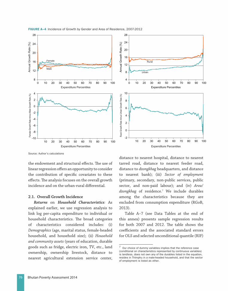
76 Bhutan Poverty Assessment 2014
the endowment and structural effects. The use of linear regression offers an opportunity to consider the contribution of specific covariates to these effects. The analysis focuses on the overall growth incidence and on the urban-rural differential.
2.1. Overall Growth IncidenceReturns on Household Characteristics: As
explained earlier, we use regression analysis to link log per-capita expenditure to individual or household characteristics. The broad categories of characteristics considered includes: (i) Demographics (age, marital status, female-headed household, and household size); (ii) Household and community assets (years of education, durable goods such as fridge, electric iron, TV, etc., land ownership, ownership livestock, distance to nearest agricultural extension service center,
distance to nearest hospital, distance to nearest tarred road, distance to nearest feeder road, distance to dzongkhag headquarters, and distance to nearest bank); (iii) Sector of employment (primary, secondary, non-public services, public sector, and non-paid labour); and (iv) Area/dzongkhag of residence.7 We include durables among the characteristics because they are excluded from consumption expenditure (RGoB, 2013).
Table A–7 (see Data Tables at the end of this annex) presents sample regression results for both 2007 and 2012. The table shows the coefficients and the associated standard errors for OLS and selected unconditional quantile (RIF)
7 Our choice of dummy variables implies that the reference case (conditional on characteristics represented by continuous variables) is landless, does not own any of the durables listed in the equation, resides in Thimphu in a male-headed household, and that the sector of employment is listed as other.
FIguRE A–4 Incidence of Growth by Gender and Area of Residence, 2007-2012
8
12
16
20
24
28
0 10 20 30 40 50 60 70 80 90 100Expenditure Percentiles Expenditure Percentiles
Male
Female
Ann
ual G
row
th R
ate
(%)
Ann
ual G
row
th R
ate
(%)
Fema
le Gr
owth
Rate
minu
s Male
Gro
wth R
ate (%
)
Rura
l Gro
wth R
ate m
inus U
rban
Gro
wth R
ate (%
)
-10
-8
-6
-4
-2
0
2
4
10 20 30 40 50 60 70 80 90 100
4
8
12
16
20
24
28
0 10 20 30 40 50 60 70 80 90 100
Rural
Urban
-2
0
2
4
6
8
10
10 20 30 40 50 60 70 80 90 100
Source: Author’s calculations

77Bhutan Poverty Assessment 2014
regressions.8 Focusing first on OLS results, we find that among the demographic characteristics age and household size are the only covariates that are statistically significant. However, the effect of age is very small. As expected, household size is negatively correlated with per capita expenditure. Similarly, returns on education are positive and statistically significant. Most durable goods have a positive and significant effect on per-capita expenditure. But, ownership of a heater water boiler, rice cooker, and TV does not have the same sign across both datasets (negative in 2007 and positive in 2012). Similarly, land ownership switches from negative in 2007 to positive in 2012. We interpret this as an improvement in productivity, possibly linked to availability of complementary inputs and the development of road infrastructure.
On average, the returns on employment in the primary sector were significant and negative in 2007, but insignificant in 2012. The returns on employment in the secondary sector are statistically significant in both years, but positive only in 2012. Employment in the public sector does not seem to pay. The associated regression coefficient is negative and significant only in 2007. Employment in the non-public service sector is associated with positive and significant coefficient only in 2012. Residence in the rural area is negatively correlated with the welfare indicator. This negative correlation is statistically significant in 2007. Similarly, most dzongkhag
8 RIF stands for Recentered Influence Function. The influence function of a distributional statistic such as the mean or a quantile measures the impact on the statistic of a small change in the underlying distribution. The RIF is equal to the statistic in question plus its influence function, if it exists (Firpo et al., 2009). Because the expected value of the influence function is equal to zero, the RIF offers a simple way of linking a distributional statistic to individual or household characteristics, using the conditional expectation function (CEF). Oaxaca-Blinder decomposition requires unconditional expectation of the statistic of interest. This can be obtained by applying the law of iterated expectations to the RIF regression. As it turns out, the OLS implements the RIF regression for the unconditional mean of an outcome variable. See Essama-Nssah and Lambert (2013) for the derivation of RIFs for a variety of distributional statistics used in policy impact evaluation.
dummies are negative and statistically significant coefficients. These returns are relative to the omitted dzongkhag (i.e., Thimphu). We note that the coefficients for Gasa, Paro, and Trashi-Yangtse are positive but not significant in 2007 while that of Tsirang is positive and significant.
Composition versus Structure: The OLS estimates give only average impacts for the characteristics under consideration. We will therefore base the decomposition of the GIC on the results from RIF regressions in order to appreciate the extent of heterogeneity in these impacts across quantiles. This decomposition is analogous to growth accounting, which is an exercise designed to identify the key drivers of economic growth by decomposing growth in output into two components: one attributable to changes in factors of production such as physical and human capital, and a residual not related to changes in output levels. This residual is commonly taken to stand for change in total factor productivity (TFP). We consider the living standard of an individual or a household as an outcome of participation in the life of society. This outcome is a function of individual characteristics and returns on those characteristics. We therefore use the analogy between growth accounting and the counterfactual decomposition of the GIC considered to link the endowment effect to notion of accumulation (of factors of production) and we take the structural effect to be an indicator of productivity in socioeconomic interaction. Accumulation and productivity are indeed the two basic ideas that structure the study of economic growth.
Figure A–5 shows a decomposition of the total variation in the distribution of log per capita expenditure (essentially the GIC) into two components. The first component is due to changes in the distribution of characteristics while the second represents the contribution of changes in the distribution of returns on those
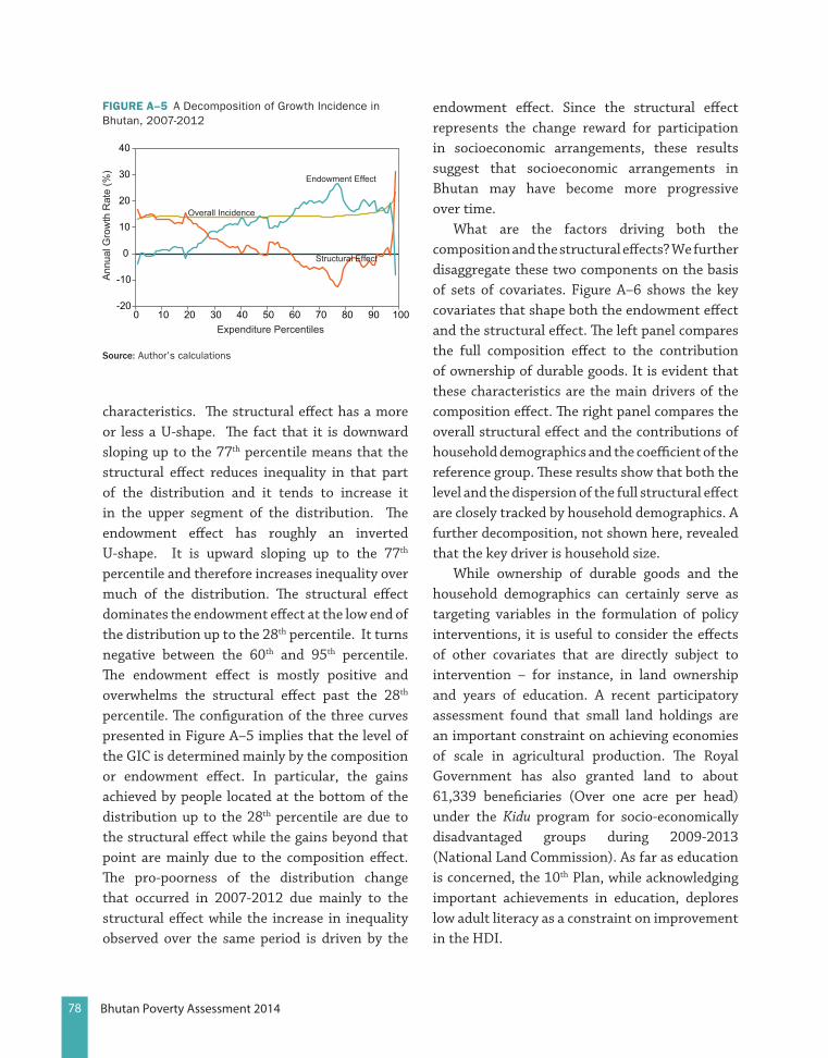
78 Bhutan Poverty Assessment 2014
characteristics. The structural effect has a more or less a U-shape. The fact that it is downward sloping up to the 77th percentile means that the structural effect reduces inequality in that part of the distribution and it tends to increase it in the upper segment of the distribution. The endowment effect has roughly an inverted U-shape. It is upward sloping up to the 77th percentile and therefore increases inequality over much of the distribution. The structural effect dominates the endowment effect at the low end of the distribution up to the 28th percentile. It turns negative between the 60th and 95th percentile. The endowment effect is mostly positive and overwhelms the structural effect past the 28th percentile. The configuration of the three curves presented in Figure A–5 implies that the level of the GIC is determined mainly by the composition or endowment effect. In particular, the gains achieved by people located at the bottom of the distribution up to the 28th percentile are due to the structural effect while the gains beyond that point are mainly due to the composition effect. The pro-poorness of the distribution change that occurred in 2007-2012 due mainly to the structural effect while the increase in inequality observed over the same period is driven by the
endowment effect. Since the structural effect represents the change reward for participation in socioeconomic arrangements, these results suggest that socioeconomic arrangements in Bhutan may have become more progressive over time.
What are the factors driving both the composition and the structural effects? We further disaggregate these two components on the basis of sets of covariates. Figure A–6 shows the key covariates that shape both the endowment effect and the structural effect. The left panel compares the full composition effect to the contribution of ownership of durable goods. It is evident that these characteristics are the main drivers of the composition effect. The right panel compares the overall structural effect and the contributions of household demographics and the coefficient of the reference group. These results show that both the level and the dispersion of the full structural effect are closely tracked by household demographics. A further decomposition, not shown here, revealed that the key driver is household size.
While ownership of durable goods and the household demographics can certainly serve as targeting variables in the formulation of policy interventions, it is useful to consider the effects of other covariates that are directly subject to intervention – for instance, in land ownership and years of education. A recent participatory assessment found that small land holdings are an important constraint on achieving economies of scale in agricultural production. The Royal Government has also granted land to about 61,339 beneficiaries (Over one acre per head) under the Kidu program for socio-economically disadvantaged groups during 2009-2013 (National Land Commission). As far as education is concerned, the 10th Plan, while acknowledging important achievements in education, deplores low adult literacy as a constraint on improvement in the HDI.
FIguRE A–5 A Decomposition of Growth Incidence in Bhutan, 2007-2012
-20
-10
0
10
20
30
40
0 10 20 30 40 50 60 70 80 90 100Expenditure Percentiles
Overall Incidence
Endowment Effect
Structural Effect
Ann
ual G
row
th R
ate
(%)
source: Author’s calculations
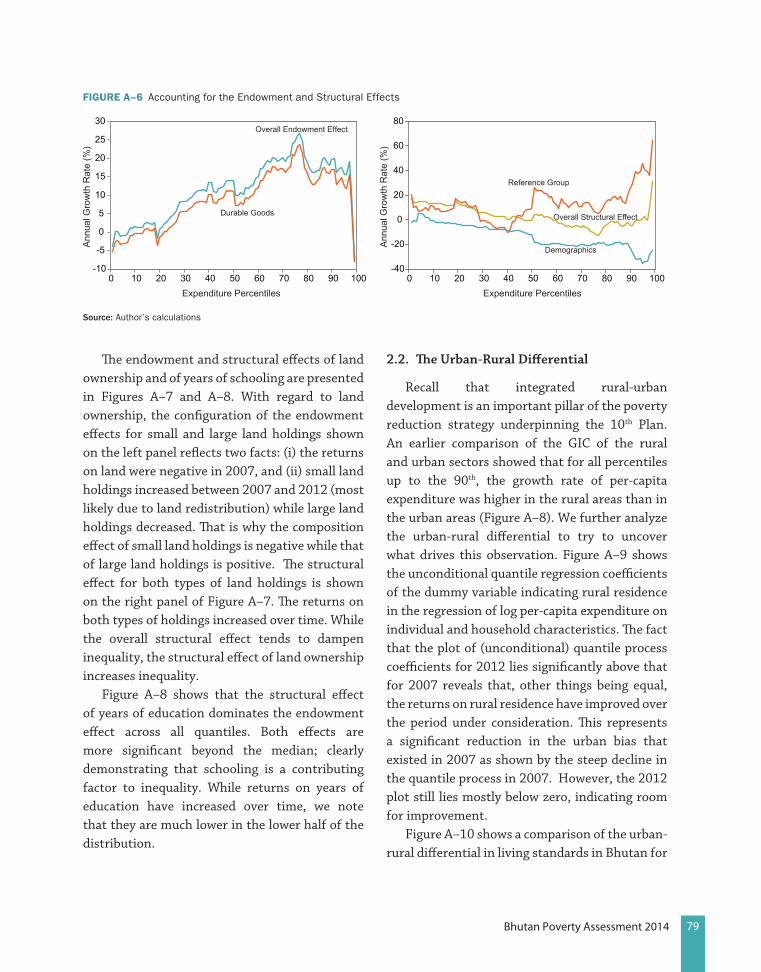
79Bhutan Poverty Assessment 2014
The endowment and structural effects of land ownership and of years of schooling are presented in Figures A–7 and A–8. With regard to land ownership, the configuration of the endowment effects for small and large land holdings shown on the left panel reflects two facts: (i) the returns on land were negative in 2007, and (ii) small land holdings increased between 2007 and 2012 (most likely due to land redistribution) while large land holdings decreased. That is why the composition effect of small land holdings is negative while that of large land holdings is positive. The structural effect for both types of land holdings is shown on the right panel of Figure A–7. The returns on both types of holdings increased over time. While the overall structural effect tends to dampen inequality, the structural effect of land ownership increases inequality.
Figure A–8 shows that the structural effect of years of education dominates the endowment effect across all quantiles. Both effects are more significant beyond the median; clearly demonstrating that schooling is a contributing factor to inequality. While returns on years of education have increased over time, we note that they are much lower in the lower half of the distribution.
2.2. The Urban-Rural Differential
Recall that integrated rural-urban development is an important pillar of the poverty reduction strategy underpinning the 10th Plan. An earlier comparison of the GIC of the rural and urban sectors showed that for all percentiles up to the 90th, the growth rate of per-capita expenditure was higher in the rural areas than in the urban areas (Figure A–8). We further analyze the urban-rural differential to try to uncover what drives this observation. Figure A–9 shows the unconditional quantile regression coefficients of the dummy variable indicating rural residence in the regression of log per-capita expenditure on individual and household characteristics. The fact that the plot of (unconditional) quantile process coefficients for 2012 lies significantly above that for 2007 reveals that, other things being equal, the returns on rural residence have improved over the period under consideration. This represents a significant reduction in the urban bias that existed in 2007 as shown by the steep decline in the quantile process in 2007. However, the 2012 plot still lies mostly below zero, indicating room for improvement.
Figure A–10 shows a comparison of the urban-rural differential in living standards in Bhutan for
FIguRE A–6 Accounting for the Endowment and Structural Effects
-10
-5
0
5
10
15
20
25
30
0 10 20 30 40 50 60 70 80 90 100
Durable Goods
Overall Endowment Effect
Overall Structural Effect
Reference Group
DemographicsAnn
ual G
row
th R
ate
(%)
Ann
ual G
row
th R
ate
(%)
-40
-20
0
20
40
60
80
0 10 20 30 40 50 60 70 80 90 100
source: Author’s calculations
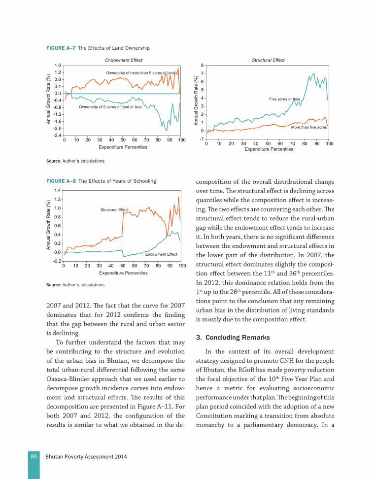
80 Bhutan Poverty Assessment 2014
2007 and 2012. The fact that the curve for 2007 dominates that for 2012 confirms the finding that the gap between the rural and urban sector is declining.
To further understand the factors that may be contributing to the structure and evolution of the urban bias in Bhutan, we decompose the total urban-rural differential following the same Oaxaca-Blinder approach that we used earlier to decompose growth incidence curves into endow-ment and structural effects. The results of this decomposition are presented in Figure A–11. For both 2007 and 2012, the configuration of the results is similar to what we obtained in the de-
composition of the overall distributional change over time. The structural effect is declining across quantiles while the composition effect is increas-ing. The two effects are countering each other. The structural effect tends to reduce the rural-urban gap while the endowment effect tends to increase it. In both years, there is no significant difference between the endowment and structural effects in the lower part of the distribution. In 2007, the structural effect dominates slightly the composi-tion effect between the 11th and 36th percentiles. In 2012, this dominance relation holds from the 1st up to the 26th percentile. All of these considera-tions point to the conclusion that any remaining urban bias in the distribution of living standards is mostly due to the composition effect.
3. Concluding remarks
In the context of its overall development strategy designed to promote GNH for the people of Bhutan, the RGoB has made poverty reduction the focal objective of the 10th Five Year Plan and hence a metric for evaluating socioeconomic performance under that plan. The beginning of this plan period coincided with the adoption of a new Constitution marking a transition from absolute monarchy to a parliamentary democracy. In a
FIguRE A–7 The Effects of Land Ownership
-2.4-2.0-1.6-1.2-0.8-0.40.00.40.81.21.6
0 10 20 30 40 50 60 70 80 90 100Expenditure Percentiles Expenditure Percentiles
Endowment Effect Structural Effect
Ownership of 5 acres of land or less
More than five acres
Ownership of more than 5 acres of land
Five acres or less
Ann
ual G
row
th R
ate
(%)
Ann
ual G
row
th R
ate
(%)
-1
0
1
2
3
4
5
6
7
8
0 10 20 30 40 50 60 70 80 90 100
source: Author’s calculations
FIguRE A–8 The Effects of Years of Schooling
-0.2
0.0
0.2
0.4
0.6
0.8
1.0
1.2
1.4
0 10 20 30 40 50 60 70 80 90 100Expenditure Percentiles
Structural Effect
Endowment Effect
Ann
ual G
row
th R
ate
(%)
source: Author’s calculations
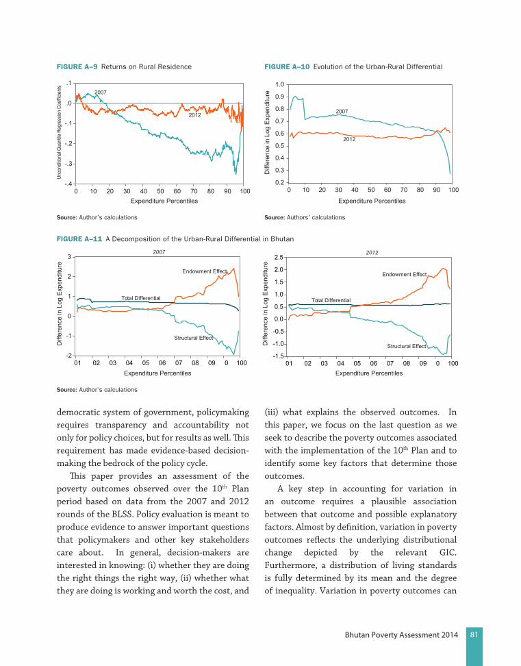
81Bhutan Poverty Assessment 2014
democratic system of government, policymaking requires transparency and accountability not only for policy choices, but for results as well. This requirement has made evidence-based decision-making the bedrock of the policy cycle.
This paper provides an assessment of the poverty outcomes observed over the 10th Plan period based on data from the 2007 and 2012 rounds of the BLSS. Policy evaluation is meant to produce evidence to answer important questions that policymakers and other key stakeholders care about. In general, decision-makers are interested in knowing: (i) whether they are doing the right things the right way, (ii) whether what they are doing is working and worth the cost, and
(iii) what explains the observed outcomes. In this paper, we focus on the last question as we seek to describe the poverty outcomes associated with the implementation of the 10th Plan and to identify some key factors that determine those outcomes.
A key step in accounting for variation in an outcome requires a plausible association between that outcome and possible explanatory factors. Almost by definition, variation in poverty outcomes reflects the underlying distributional change depicted by the relevant GIC. Furthermore, a distribution of living standards is fully determined by its mean and the degree of inequality. Variation in poverty outcomes can
FIguRE A–9 Returns on Rural Residence
-.4
-.3
-.2
-.1
.0
.1
0 10 20 30 40 50 60 70 80 90 100Expenditure Percentiles
2007
2012
Unco
nditio
nal Q
uanti
le Re
gres
sion C
oeffic
ients
source: Author’s calculations
FIguRE A–10 Evolution of the Urban-Rural Differential
0.2
0.3
0.4
0.5
0.6
0.7
0.8
0.9
1.0
0 10 20 30 40 50 60 70 80 90 100
Expenditure Percentiles
2007
2012
Diff
eren
ce in
Log
Exp
endi
ture
source: Authors’ calculations
FIguRE A–11 A Decomposition of the Urban-Rural Differential in Bhutan
2007 2012
Total Differential Total Differential
Endowment Effect Endowment Effect
Structural EffectStructural Effect
-2
-1
0
1
2
3
01 02 03 04 05 06 07 08 09 0 100
Diff
eren
ce in
Log
Exp
endi
ture
Diff
eren
ce in
Log
Exp
endi
ture
-1.5
-1.0
-0.5
0.0
0.5
1.0
1.5
2.0
2.5
01 02 03 04 05 06 07 08 09 0 100
source: Author’s calculations

82 Bhutan Poverty Assessment 2014
therefore be seen as driven by these factors as well. However, it is hard to target distributional statistics such as the mean or a measure of inequality with policy instruments. This creates the need for deeper analysis linking distributional change to individual or household characteristics. The living standard of an individual (or household) is a pay-off from participation in the life of society subject to individual endowments and the circumstances that determine the returns on those endowments from social interaction. This consideration provides a theoretical basis for the link between distributional statistics and individual characteristics. We rely on the Conditional Expectation Function to implement this link empirically. The identification of sources of variation in poverty outcomes is based on counterfactual decomposition.
Analysis of the 2007 and 2012 rounds of the BLSS shows that real household per-capita expenditure more than doubled in the span of five years. This doubling of per-capita expenditure was also accompanied by an increase in relative inequality; the overall Gini coefficient increased from 33.37 percent in 2007 to 38.81 percent in 2012. We find that a wide class of poverty measures (e.g., FGT and Watts) would agree that poverty in Bhutan declined between 2007 and 2012 – the poverty incidence fell from 23 percent to 12 percent. These findings suggest that the implementation of the 10th Plan has been pro-poor to a certain extent. The exact extent depends on the chosen standard of evaluation. If one adopts a relative standard based on the annual growth rate of the average per-capita expenditure, then the conclusion would be that the observed distributional change was not pro-poor enough.
A counterfactual decomposition of the overall GIC into the endowment and structural effects shows that the level of the GIC is determined mainly by the endowment effect. Furthermore, the pro-poorness of the distribution change that occurred in 2007-2012 is due mainly to the structural effect while the increase in inequality observed over the same period is driven by the endowment effect. Since the structural effect represents the change reward for participation in socioeconomic arrangements, these results suggest that socioeconomic arrangements in Bhutan may have become more progressive over time. A closer look at some particular covariates revealed that: (i) the endowment effect is accounted for mostly by the ownership of durable goods; (ii) the structural effect is driven by demographic factors; (iii) the returns on land improved between 2007 and 2012; (iv) the structural effect of land ownership tends to increase inequality; and (v) schooling is a contributing factor to inequality through both its endowment and structural effects.
A similar decomposition analysis of the urban-rural differential confirms that the gap between the rural and urban sectors has been shrinking over time. This reduction is driven by the structural effect. Much of the remaining urban bias is accounted for by the composition effect. In any case, these findings suggest that the policy of integrated rural urban development may be working.
The overall conclusion emerging from this analysis is that the implementation of the 10th Plan has been pro-poor. This result is most likely due to that fact that socioeconomic arrangements in Bhutan have become more progressive.
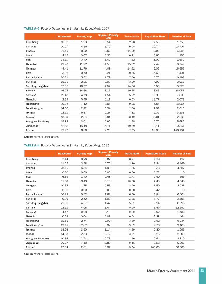
83Bhutan Poverty Assessment 2014
TABlE A–3 Poverty Outcomes in Bhutan, by Dzongkhag, 2007
Headcount Poverty gap Squared Poverty gap Watts Index Population Share Number of Poor
Bumthang 10.93 1.93 0.54 2.28 2.55 1,753
Chhukha 20.27 4.86 1.70 6.08 10.74 13,704
Dagana 31.10 8.82 3.62 11.69 3.00 5,867
Gasa 4.15 0.67 0.20 0.81 0.60 156
haa 13.19 3.49 1.60 4.82 1.99 1,650
Lhuentse 42.97 11.92 4.58 15.32 2.49 6,749
monggar 44.41 11.76 4.08 14.62 6.06 16,959
Paro 3.95 0.70 0.21 0.85 5.63 1,401
Pema Gatshel 26.21 5.82 1.79 7.06 3.76 6,197
Punakha 15.65 3.21 0.98 3.90 4.03 3,966
samdrup Jongkhar 37.98 10.97 4.57 14.66 5.55 13,270
samtse 46.76 14.68 6.17 19.55 8.85 26,056
sarpang 19.43 4.78 1.54 5.82 6.38 7,809
thimphu 2.39 0.46 0.11 0.53 13.77 2,073
trashigang 29.28 7.12 2.63 9.08 7.58 13,966
trashi yangtse 14.33 2.22 0.54 2.56 2.89 2,610
trongsa 22.15 6.17 2.27 7.82 2.32 3,231
tsirang 13.89 2.84 0.91 3.49 3.01 2,635
Wangdue Phodrang 15.84 3.01 0.92 3.65 5.70 5,685
Zhemgang 52.86 15.18 5.71 19.39 3.11 10,364
Bhutan 23.20 6.06 2.26 7.75 100.00 146,101
source: Author’s calculations
TABlE A–4 Poverty Outcomes in Bhutan, by Dzongkhag, 2012
Headcount Poverty gap Squared Poverty gap Watts Index Population Share Number of Poor
Bumthang 3.44 0.26 0.02 0.27 2.19 437
Chhukha 11.25 2.28 0.75 2.80 9.44 6,169
Dagana 25.10 5.84 1.98 7.25 3.33 4,857
Gasa 0.00 0.00 0.00 0.00 0.52 0
haa 6.39 1.40 0.48 1.73 1.50 555
Lhuentse 31.89 8.43 3.18 10.78 2.45 4,545
monggar 10.54 1.75 0.56 2.20 6.59 4,036
Paro 0.00 0.00 0.00 0.00 5.42 0
Pema Gatshel 26.88 5.52 1.68 6.70 3.84 6,004
Punakha 9.99 2.52 1.00 3.28 3.77 2,191
samdrup Jongkhar 21.01 4.57 1.47 5.61 5.24 6,393
samtse 22.16 4.68 1.44 5.69 9.46 12,192
sarpang 4.17 0.68 0.19 0.80 5.92 1,436
thimphu 0.52 0.04 0.01 0.04 15.38 464
trashigang 11.52 2.74 0.93 3.39 7.52 5,034
trashi yangtse 13.48 2.82 0.99 3.52 2.76 2,165
trongsa 14.93 3.50 1.14 4.29 2.30 1,995
tsirang 14.83 2.53 0.72 3.01 3.26 2,809
Wangdue Phodrang 10.94 2.34 0.79 2.96 5.84 3,716
Zhemgang 26.27 7.18 2.88 9.41 3.28 5,006
Bhutan 12.04 2.61 0.87 3.24 100.00 70,005
source: Author’s calculations

84 Bhutan Poverty Assessment 2014
TABlE A–5 Inequality in Distribution of per-capita Expenditure, by Dzongkhag, 2007
gini Atkinson (1) Atkinson (2) Mean log Deviation Theil Variance log per capita Expenditure
Bumthang 30.41 14.42 24.22 15.57 18.90 26.53
Chhukha 37.74 21.08 36.01 23.68 24.99 44.67
Dagana 30.12 14.14 26.66 15.24 15.16 30.89
Gasa 25.80 10.22 18.57 10.78 11.46 20.34
haa 28.82 13.08 25.06 14.02 13.99 28.42
Lhuentse 29.86 13.60 23.71 14.62 16.49 26.54
monggar 32.83 15.79 26.35 17.18 19.33 30.25
Paro 31.03 14.29 25.07 15.41 16.42 28.76
Pema Gatshel 27.89 11.74 21.31 12.48 12.98 23.98
Punakha 36.06 18.98 30.94 21.04 24.14 36.29
samdrup Jongkhar 39.06 22.22 37.11 25.13 27.42 45.98
samtse 37.31 20.29 33.95 22.67 24.85 41.18
sarpang 31.10 14.51 25.85 15.67 16.36 29.95
thimphu 31.51 15.23 27.39 16.52 17.69 31.45
trashigang 31.85 15.51 26.47 16.85 19.36 29.83
trashi yangtse 28.08 12.00 21.05 12.78 14.34 23.26
trongsa 34.85 18.17 31.78 20.05 21.05 38.25
tsirang 32.97 16.50 27.09 18.04 21.77 30.27
Wangdue Phodrang 32.29 15.59 26.62 16.94 18.92 30.46
Zhemgang 36.58 19.51 30.70 21.71 26.60 35.25
Bhutan 38.09 21.31 36.08 23.96 25.76 44.54
source: Author’s calculations
TABlE A–6 Inequality in Distribution of per-capita Expenditure, by Dzongkhag, 2012
gini Atkinson (1) Atkinson (2) Mean log Deviation Theil Variance log per capita Expenditure
Bumthang 29.67 13.44 23.40 14.43 15.92 26.31
Chhukha 35.90 19.05 32.24 21.14 23.37 38.40
Dagana 28.84 12.81 23.23 13.70 14.42 26.25
Gasa 38.93 22.31 33.72 25.25 31.76 39.07
haa 33.58 16.93 29.59 18.55 19.69 34.87
Lhuentse 37.75 20.61 34.38 23.08 24.53 42.40
monggar 33.48 16.97 28.80 18.60 21.71 32.59
Paro 33.74 17.32 27.99 19.01 23.89 31.11
Pema Gatshel 24.78 9.44 17.45 9.92 10.34 19.07
Punakha 34.63 18.29 32.43 20.20 21.54 38.54
samdrup Jongkhar 41.87 25.17 39.68 28.99 34.95 49.01
samtse 35.70 19.05 30.28 21.14 26.48 34.20
sarpang 25.58 10.02 18.46 10.56 10.99 20.34
thimphu 34.84 17.90 29.62 19.72 22.74 34.32
trashigang 31.75 15.21 27.08 16.50 17.42 31.38
trashi yangtse 34.79 17.93 29.50 19.76 23.20 33.94
trongsa 37.18 20.33 34.51 22.73 24.27 42.30
tsirang 34.80 17.85 28.75 19.66 23.57 32.80
Wangdue Phodrang 31.28 15.41 27.64 16.74 19.25 30.80
Zhemgang 30.88 15.10 27.15 16.36 17.87 30.94
Bhutan 38.75 22.02 36.32 24.87 28.44 44.09
source: Author’s calculations
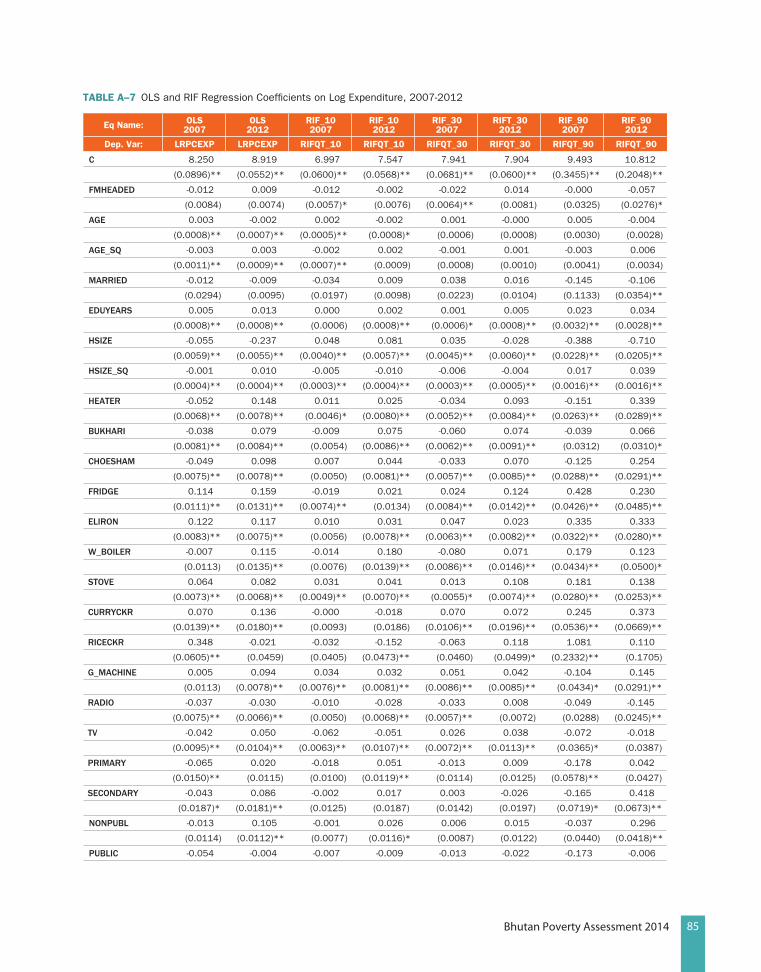
85Bhutan Poverty Assessment 2014
TABlE A–7 OLS and RIF Regression Coefficients on Log Expenditure, 2007-2012
Eq Name: OlS2007
OlS2012
RIF_102007
RIF_102012
RIF_302007
RIFT_302012
RIF_902007
RIF_902012
Dep. Var: lRPCEXP lRPCEXP RIFQT_10 RIFQT_10 RIFQT_30 RIFQT_30 RIFQT_90 RIFQT_90
C 8.250 8.919 6.997 7.547 7.941 7.904 9.493 10.812
(0.0896)** (0.0552)** (0.0600)** (0.0568)** (0.0681)** (0.0600)** (0.3455)** (0.2048)**
FmheaDeD -0.012 0.009 -0.012 -0.002 -0.022 0.014 -0.000 -0.057
(0.0084) (0.0074) (0.0057)* (0.0076) (0.0064)** (0.0081) (0.0325) (0.0276)*
aGe 0.003 -0.002 0.002 -0.002 0.001 -0.000 0.005 -0.004
(0.0008)** (0.0007)** (0.0005)** (0.0008)* (0.0006) (0.0008) (0.0030) (0.0028)
aGe_sQ -0.003 0.003 -0.002 0.002 -0.001 0.001 -0.003 0.006
(0.0011)** (0.0009)** (0.0007)** (0.0009) (0.0008) (0.0010) (0.0041) (0.0034)
marrIeD -0.012 -0.009 -0.034 0.009 0.038 0.016 -0.145 -0.106
(0.0294) (0.0095) (0.0197) (0.0098) (0.0223) (0.0104) (0.1133) (0.0354)**
eDuyears 0.005 0.013 0.000 0.002 0.001 0.005 0.023 0.034
(0.0008)** (0.0008)** (0.0006) (0.0008)** (0.0006)* (0.0008)** (0.0032)** (0.0028)**
hsIZe -0.055 -0.237 0.048 0.081 0.035 -0.028 -0.388 -0.710
(0.0059)** (0.0055)** (0.0040)** (0.0057)** (0.0045)** (0.0060)** (0.0228)** (0.0205)**
hsIZe_sQ -0.001 0.010 -0.005 -0.010 -0.006 -0.004 0.017 0.039
(0.0004)** (0.0004)** (0.0003)** (0.0004)** (0.0003)** (0.0005)** (0.0016)** (0.0016)**
heater -0.052 0.148 0.011 0.025 -0.034 0.093 -0.151 0.339
(0.0068)** (0.0078)** (0.0046)* (0.0080)** (0.0052)** (0.0084)** (0.0263)** (0.0289)**
BuKharI -0.038 0.079 -0.009 0.075 -0.060 0.074 -0.039 0.066
(0.0081)** (0.0084)** (0.0054) (0.0086)** (0.0062)** (0.0091)** (0.0312) (0.0310)*
Choesham -0.049 0.098 0.007 0.044 -0.033 0.070 -0.125 0.254
(0.0075)** (0.0078)** (0.0050) (0.0081)** (0.0057)** (0.0085)** (0.0288)** (0.0291)**
FrIDGe 0.114 0.159 -0.019 0.021 0.024 0.124 0.428 0.230
(0.0111)** (0.0131)** (0.0074)** (0.0134) (0.0084)** (0.0142)** (0.0426)** (0.0485)**
eLIron 0.122 0.117 0.010 0.031 0.047 0.023 0.335 0.333
(0.0083)** (0.0075)** (0.0056) (0.0078)** (0.0063)** (0.0082)** (0.0322)** (0.0280)**
W_BoILer -0.007 0.115 -0.014 0.180 -0.080 0.071 0.179 0.123
(0.0113) (0.0135)** (0.0076) (0.0139)** (0.0086)** (0.0146)** (0.0434)** (0.0500)*
stove 0.064 0.082 0.031 0.041 0.013 0.108 0.181 0.138
(0.0073)** (0.0068)** (0.0049)** (0.0070)** (0.0055)* (0.0074)** (0.0280)** (0.0253)**
CurryCKr 0.070 0.136 -0.000 -0.018 0.070 0.072 0.245 0.373
(0.0139)** (0.0180)** (0.0093) (0.0186) (0.0106)** (0.0196)** (0.0536)** (0.0669)**
rICeCKr 0.348 -0.021 -0.032 -0.152 -0.063 0.118 1.081 0.110
(0.0605)** (0.0459) (0.0405) (0.0473)** (0.0460) (0.0499)* (0.2332)** (0.1705)
G_maChIne 0.005 0.094 0.034 0.032 0.051 0.042 -0.104 0.145
(0.0113) (0.0078)** (0.0076)** (0.0081)** (0.0086)** (0.0085)** (0.0434)* (0.0291)**
raDIo -0.037 -0.030 -0.010 -0.028 -0.033 0.008 -0.049 -0.145
(0.0075)** (0.0066)** (0.0050) (0.0068)** (0.0057)** (0.0072) (0.0288) (0.0245)**
tv -0.042 0.050 -0.062 -0.051 0.026 0.038 -0.072 -0.018
(0.0095)** (0.0104)** (0.0063)** (0.0107)** (0.0072)** (0.0113)** (0.0365)* (0.0387)
PrImary -0.065 0.020 -0.018 0.051 -0.013 0.009 -0.178 0.042
(0.0150)** (0.0115) (0.0100) (0.0119)** (0.0114) (0.0125) (0.0578)** (0.0427)
seConDary -0.043 0.086 -0.002 0.017 0.003 -0.026 -0.165 0.418
(0.0187)* (0.0181)** (0.0125) (0.0187) (0.0142) (0.0197) (0.0719)* (0.0673)**
nonPuBL -0.013 0.105 -0.001 0.026 0.006 0.015 -0.037 0.296
(0.0114) (0.0112)** (0.0077) (0.0116)* (0.0087) (0.0122) (0.0440) (0.0418)**
PuBLIC -0.054 -0.004 -0.007 -0.009 -0.013 -0.022 -0.173 -0.006
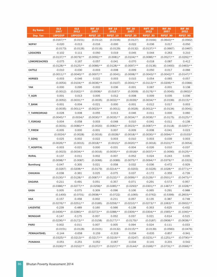
86 Bhutan Poverty Assessment 2014
Eq Name: OlS2007
OlS2012
RIF_102007
RIF_102012
RIF_302007
RIFT_302012
RIF_902007
RIF_902012
Dep. Var: lRPCEXP lRPCEXP RIFQT_10 RIFQT_10 RIFQT_30 RIFQT_30 RIFQT_90 RIFQT_90
(0.0167)** (0.0151) (0.0112) (0.0156) (0.0127) (0.0164) (0.0643)** (0.0562)
noPay -0.020 -0.013 -0.016 -0.000 -0.022 -0.036 0.017 -0.050
(0.0173) (0.0126) (0.0116) (0.0129) (0.0132) (0.0137)** (0.0667) (0.0467)
LD5aCres -0.102 0.111 -0.050 0.019 -0.045 0.044 -0.263 0.210
(0.0137)** (0.0079)** (0.0092)** (0.0081)* (0.0104)** (0.0086)** (0.0527)** (0.0292)**
LDmore5aCres -0.075 0.167 -0.057 -0.041 -0.070 -0.018 -0.087 0.412
(0.0128)** (0.0125)** (0.0086)** (0.0128)** (0.0097)** (0.0136) (0.0493) (0.0463)**
CattLe -0.010 -0.030 -0.003 -0.008 -0.009 -0.050 -0.017 -0.066
(0.0011)** (0.0040)** (0.0007)** (0.0041) (0.0008)** (0.0043)** (0.0042)** (0.0147)**
horses -0.003 -0.046 0.022 0.003 0.015 0.054 -0.065 -0.057
(0.0054) (0.0104)** (0.0036)** (0.0107) (0.0041)** (0.0113)** (0.0206)** (0.0384)
yaK -0.000 0.095 -0.002 0.036 -0.001 0.067 -0.001 0.138
(0.0012) (0.0162)** (0.0008)* (0.0167)* (0.0009) (0.0176)** (0.0045) (0.0602)*
t_aGrI 0.001 0.013 0.005 0.012 -0.008 0.009 0.035 0.036
(0.0052) (0.0031)** (0.0035) (0.0032)** (0.0039)* (0.0034)** (0.0199) (0.0115)**
t_BanK -0.001 -0.004 -0.021 0.000 -0.001 -0.012 0.017 0.003
(0.0035) (0.0011)** (0.0023)** (0.0011) (0.0026) (0.0012)** (0.0134) (0.0041)
t_tarreDroaD -0.028 0.008 -0.055 0.013 -0.046 -0.011 0.000 0.060
(0.0045)** (0.0034)* (0.0030)** (0.0035)** (0.0034)** (0.0036)** (0.0175) (0.0125)**
t_FDroaD 0.004 -0.058 0.003 -0.048 0.010 -0.041 -0.011 -0.138
(0.0031) (0.0080)** (0.0020) (0.0082)** (0.0023)** (0.0087)** (0.0118) (0.0297)**
t_FIreW -0.005 0.000 -0.001 0.007 -0.009 -0.008 -0.041 0.023
(0.0024)* (0.0028) (0.0016) (0.0028)* (0.0018)** (0.0030)** (0.0094)** (0.0103)*
t_DZhQ -0.025 -0.002 -0.022 0.003 -0.010 0.003 -0.039 0.003
(0.0026)** (0.0015) (0.0018)** (0.0015)* (0.0020)** (0.0016) (0.0101)** (0.0054)
t_hosPItaL -0.003 -0.021 0.000 -0.031 -0.004 -0.026 0.010 -0.037
(0.0023) (0.0034)** (0.0016) (0.0035)** (0.0018)* (0.0037)** (0.0090) (0.0125)**
ruraL -0.137 -0.011 0.002 -0.007 -0.052 0.024 -0.243 0.035
(0.0098)** (0.0087) (0.0066) (0.0089) (0.0075)** (0.0094)** (0.0379)** (0.0323)
Bumthang -0.047 -0.305 0.021 -0.058 0.032 -0.036 -0.472 -0.929
(0.0267) (0.0208)** (0.0179) (0.0214)** (0.0203) (0.0226) (0.1028)** (0.0771)**
ChhuKha -0.038 -0.361 0.025 -0.075 0.037 -0.172 -0.359 -0.739
(0.0130)** (0.0128)** (0.0087)** (0.0132)** (0.0099)** (0.0139)** (0.0501)** (0.0475)**
DaGana -0.211 -0.491 0.051 -0.357 -0.071 -0.291 -0.573 -0.957
(0.0386)** (0.0277)** (0.0258)* (0.0285)** (0.0293)* (0.0301)** (0.1487)** (0.1028)**
Gasa 0.005 -0.075 0.309 -0.096 0.106 -0.065 0.291 -0.988
(0.1400) (0.0701) (0.0938)** (0.0722) (0.1065) (0.0762) (0.5399) (0.2603)**
haa -0.157 -0.458 -0.002 -0.211 -0.057 -0.135 -0.387 -0.748
(0.0276)** (0.0251)** (0.0185) (0.0259)** (0.0210)** (0.0273)** (0.1063)** (0.0932)**
Lhuentse -0.239 -0.489 0.160 -0.566 -0.138 -0.353 -0.625 -0.432
(0.0406)** (0.0280)** (0.0272)** (0.0288)** (0.0309)** (0.0304)** (0.1565)** (0.1040)**
monGGar -0.147 -0.175 -0.007 0.052 0.037 0.021 -0.614 -0.515
(0.0236)** (0.0172)** (0.0158) (0.0177)** (0.0179)* (0.0187) (0.0908)** (0.0638)**
Paro 0.002 -0.011 0.007 0.005 0.094 0.024 -0.111 -0.033
(0.0151) (0.0128) (0.0101) (0.0132) (0.0115)** (0.0139) (0.0583) (0.0476)
PemaGatsheL -0.144 -0.658 0.159 -0.319 0.034 -0.635 -0.857 -0.941
(0.0325)** (0.0213)** (0.0217)** (0.0219)** (0.0247) (0.0231)** (0.1251)** (0.0790)**
PunaKha -0.051 -0.251 0.052 -0.067 -0.034 -0.141 -0.201 -0.542
(0.0190)** (0.0152)** (0.0127)** (0.0157)** (0.0144)* (0.0166)** (0.0731)** (0.0566)**

87Bhutan Poverty Assessment 2014
Eq Name: OlS2007
OlS2012
RIF_102007
RIF_102012
RIF_302007
RIFT_302012
RIF_902007
RIF_902012
Dep. Var: lRPCEXP lRPCEXP RIFQT_10 RIFQT_10 RIFQT_30 RIFQT_30 RIFQT_90 RIFQT_90
samDruPJ -0.072 -0.088 -0.044 -0.025 -0.042 0.003 -0.104 -0.151
(0.0199)** (0.0180)** (0.0134)** (0.0185) (0.0152)** (0.0195) (0.0768) (0.0668)*
samtse -0.223 -0.354 -0.052 -0.021 0.008 -0.099 -0.875 -0.722
(0.0172)** (0.0167)** (0.0115)** (0.0172) (0.0131) (0.0182)** (0.0662)** (0.0622)**
sarPanG -0.121 -0.322 0.058 0.073 0.023 -0.048 -0.531 -0.917
(0.0164)** (0.0149)** (0.0110)** (0.0154)** (0.0125) (0.0162)** (0.0633)** (0.0554)**
trashIGanG -0.185 -0.414 -0.039 -0.018 0.016 -0.215 -0.582 -1.092
(0.0191)** (0.0153)** (0.0128)** (0.0158) (0.0146) (0.0167)** (0.0738)** (0.0569)**
trashIy 0.023 -0.270 0.015 -0.192 0.046 -0.099 -0.259 -0.819
(0.0361) (0.0278)** (0.0242) (0.0286)** (0.0274) (0.0302)** (0.1390) (0.1030)**
tronGsa -0.059 -0.244 0.010 -0.162 -0.045 -0.209 -0.618 -0.357
(0.0338) (0.0260)** (0.0227) (0.0268)** (0.0257) (0.0283)** (0.1304)** (0.0966)**
tsIranG 0.106 -0.291 -0.005 -0.112 0.049 -0.122 0.367 -0.802
(0.0381)** (0.0249)** (0.0255) (0.0257)** (0.0290) (0.0271)** (0.1470)* (0.0926)**
WanGDueP -0.043 -0.264 -0.006 -0.061 0.036 -0.009 -0.305 -0.655
(0.0185)* (0.0156)** (0.0124) (0.0161)** (0.0141)* (0.0170) (0.0714)** (0.0581)**
ZhemGanG -0.087 -0.359 0.037 0.039 0.041 0.100 -0.182 -0.773
(0.0322)** (0.0233)** (0.0216) (0.0239) (0.0245) (0.0253)** (0.1243) (0.0863)**
observations: 13155 21190 13155 21190 13155 21190 13155 21190
r-squared: 0.3115 0.4461 0.1799 0.1401 0.2419 0.2404 0.1525 0.2123
F-statistic: 105.8402 303.9084 51.3155 61.5096 74.6442 119.4643 42.0930 101.7009
source: Author’s calculations

88 Bhutan Poverty Assessment 2014
Annex B: Poverty Dynamics with synthetic Panels – Framework and results
overview of synthetic Panel method9
Let xij be a vector of household characteristics observed in survey round j (j= 1 or 2) that are also observed in the other survey round for household i, I= 1,… N. These household characteristics can include such time-invariant variables as ethnicity, religion, language, place of birth, parental education, and others available in the survey. The vector xij can also include deterministic variables such as age (which given the value in one survey round can then be determined given the time interval between the two survey rounds), or time-varying household characteristics if retrospective questions about the round-1 values of such characteristics are asked in the second round survey. To reduce spurious changes due to changes in household composition over time, we usually restrict the estimation samples to household heads age, say 25 to 55 in the first cross section and adjust this age range accordingly in the second cross section.10
Then let yij represent household consumption or income in survey round j, j= 1 or 2. The linear projection of household consumption (or income) on household characteristics for each survey round is given by
(1)
9 We provide an overview of the synthetic panel method developed by Dang, Lanjouw, Luoto, and McKenzie (2014) and Dang and Lanjouw (2013) in this section. For more details, readers are encouraged to read the original papers.
10 This age range is usually used in traditional pseudo-panel analysis but can vary depending on the cultural and economic factors in each specific setting.
(2)
Let zj be the poverty line in period j, j= 1 or 2. We are interested in knowing such quantities as
(3a)
which represents the percentage of households that are poor in the first period but non poor in the second period (considered together for two periods), or
(3b)
which represents the percentage of poor households in the first period that escape poverty in the second period. Put differently, for the average household, quantity (3a) provides the joint probabilities of household poverty status in both periods, and quantity (3b) the conditional probabilities of household poverty status in the second period given their poverty status in the first period.
If true panel data are available, we can easily calculate the quantities in (3a) and (3b); otherwise, in the absence of such data, we have to rely on synthetic panels to study mobility. Two standard assumptions are then made to operationalize the framework to construct synthetic panel data. First, the underlying population being sampled in survey rounds 1 and 2 are assumed to be the same in terms of the household characteristics xij; more specifically, it is assumed that xi1= wxi2, and yi1|xi1
and yi1|xi2 have identical distributions. Second, �i1
and �i2 are assumed to follow a bivariate normal

89Bhutan Poverty Assessment 2014
distribution with correlation coefficient � and standard deviations and respectively.11 If � is known, quantity (3a) can be estimated by
(4)
where �2�.� stands for the bivariate normal cumulative distribution function (cdf) ) (and 𝜙2�.� stands for the bivariate normal probability density function (pdf)). Note that in equality (4), the estimated parameters obtained from data in both survey rounds are applied to data from the second survey round (x2) (or the base year) for prediction.
11 In other words, this assumption implies that households in period 2 that have similar characteristics to those of households in period 1 would have achieved the same consumption levels in period 1 or vice versa.
Since � is usually unknown in most contexts, we can first approximate the simple correlation coefficient between birth cohort-aggregated household consumption between the two surveys, then estimate � using the following formula
(5)
It is then straightforward to estimate quantity (3b) by dividing quantity (4) by
,
where ��.� stands for the univariate normal cumulative distribution function (cdf).
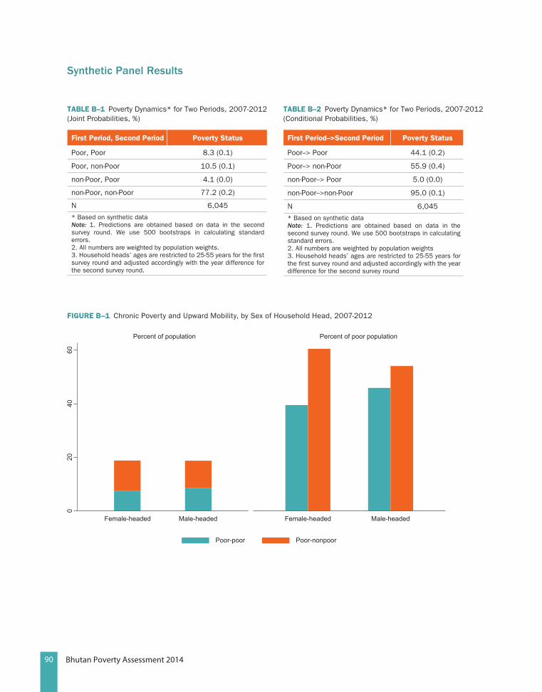
90 Bhutan Poverty Assessment 2014
synthetic Panel results
TABlE B–1 Poverty Dynamics* for Two Periods, 2007-2012 (Joint Probabilities, %)
First Period, Second Period Poverty Status
Poor, Poor 8.3 (0.1)
Poor, non-Poor 10.5 (0.1)
non-Poor, Poor 4.1 (0.0)
non-Poor, non-Poor 77.2 (0.2)
N 6,045
* Based on synthetic dataNote: 1. Predictions are obtained based on data in the second survey round. We use 500 bootstraps in calculating standard errors.2. All numbers are weighted by population weights.3. Household heads’ ages are restricted to 25-55 years for the first survey round and adjusted accordingly with the year difference for the second survey round.
TABlE B–2 Poverty Dynamics* for Two Periods, 2007-2012 (Conditional Probabilities, %)
First Period-->Second Period Poverty Status
Poor--> Poor 44.1 (0.2)
Poor--> non-Poor 55.9 (0.4)
non-Poor--> Poor 5.0 (0.0)
non-Poor-->non-Poor 95.0 (0.1)
N 6,045
* Based on synthetic dataNote: 1. Predictions are obtained based on data in the second survey round. We use 500 bootstraps in calculating standard errors.2. All numbers are weighted by population weights3. Household heads’ ages are restricted to 25-55 years for the first survey round and adjusted accordingly with the year difference for the second survey round
FIguRE B–1 Chronic Poverty and Upward Mobility, by Sex of Household Head, 2007-2012
Female-headed
Percent of poor populationPercent of population
Poor-poor Poor-nonpoor
Male-headed Female-headed Male-headed

91Bhutan Poverty Assessment 2014
FIguRE B–2 Downward Mobility by Sex of Household Head, 2007-2012
Percent of nonpoor in 2007Percent of population
Female-headed
Nonpoor-nonpoor Nonpoor-poor
Male-headed Female-headed Male-headed
FIguRE B–3 Chronic Poverty and Upward Mobility by residence area, 2007-2012
Percent of poor in 2007Percent of population
Poor-poor Poor-nonpoor
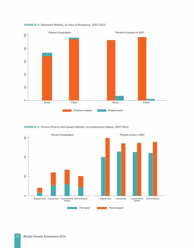
92 Bhutan Poverty Assessment 2014
FIguRE B–4 Downward Mobility, by Area of Residence, 2007-20120
2040
6080
100
Percent of nonpoor in 2007Percent of population
Nonpoor-nonpoor Nonpoor-poor
FIguRE B–5 Chronic Poverty and Upward Mobility, by Employment Status, 2007-2012
020
4060
Percent of poor in 2007Percent of population
Poor-poor Poor-nonpoor
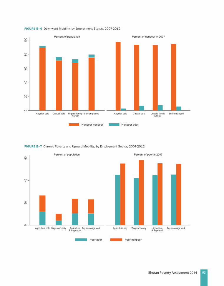
93Bhutan Poverty Assessment 2014
FIguRE B–6 Downward Mobility, by Employment Status, 2007-2012
Nonpoor-nonpoor Nonpoor-poor
020
4010
080
60
Percent of nonpoor in 2007Percent of population
FIguRE B–7 Chronic Poverty and Upward Mobility, by Employment Sector, 2007-2012
Poor-poor Poor-nonpoor
020
4060
Percent of poor in 2007Percent of population
Agriculture only Wage work only Agriculture& wage work
Any non-wage work Agriculture only Wage work only Agriculture& wage work
Any non-wage work
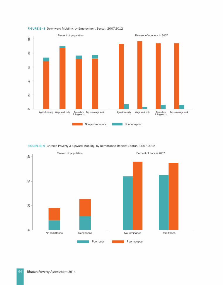
94 Bhutan Poverty Assessment 2014
FIguRE B–8 Downward Mobility, by Employment Sector, 2007-2012
Percent of population
Nonpoor-nonpoor Nonpoor-poor
Percent of nonpoor in 2007
020
4010
080
60
Agriculture only Wage work only Agriculture& wage work
Any non-wage work Agriculture only Wage work only Agriculture& wage work
Any non-wage work
FIguRE B–9 Chronic Poverty & Upward Mobility, by Remittance Receipt Status, 2007-2012
Percent of poor in 2007Percent of population
No remittance Remittance No remittance Remittance
Poor-poor Poor-nonpoor
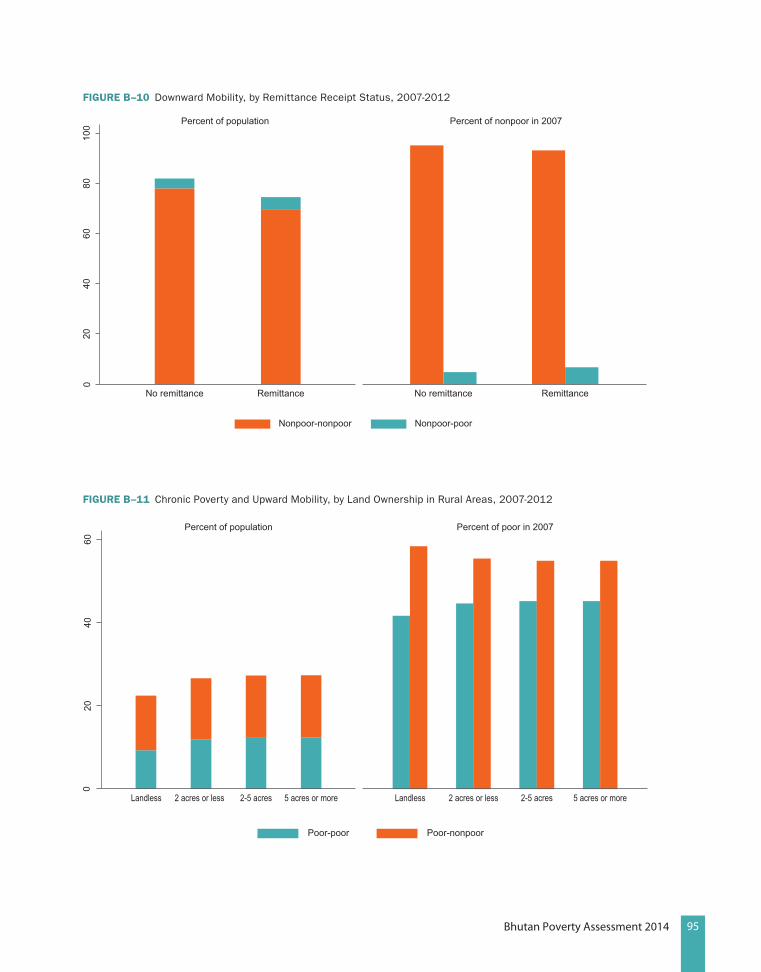
95Bhutan Poverty Assessment 2014
FIguRE B–10 Downward Mobility, by Remittance Receipt Status, 2007-20120
2040
6080
100
Percent of nonpoor in 2007Percent of population
No remittance Remittance No remittance Remittance
Nonpoor-nonpoor Nonpoor-poor
FIguRE B–11 Chronic Poverty and Upward Mobility, by Land Ownership in Rural Areas, 2007-2012
Percent of population
Poor-poor Poor-nonpoor
Percent of poor in 2007
020
4060
Landless 2 acres or less 2-5 acres 5 acres or more Landless 2 acres or less 2-5 acres 5 acres or more
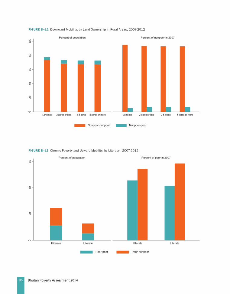
96 Bhutan Poverty Assessment 2014
FIguRE B–12 Downward Mobility, by Land Ownership in Rural Areas, 2007-2012
Percent of population
Nonpoor-nonpoor Nonpoor-poor
Percent of nonpoor in 2007
020
4010
060
80
Landless 2 acres or less 2-5 acres 5 acres or more Landless 2 acres or less 2-5 acres 5 acres or more
FIguRE B–13 Chronic Poverty and Upward Mobility, by Literacy, 2007-2012
Percent of population
Poor-poor Poor-nonpoor
Percent of poor in 2007
020
4060

97Bhutan Poverty Assessment 2014
FIguRE B–14 Downward Mobility, by Literacy, 2007-2012
Percent of population
Nonpoor-nonpoor Nonpoor-poor
Percent of nonpoor in 2007
FIguRE B–15 Chronic Poverty and Upward Mobility, Education Achievement, 2007-2012
Percent of population
Poor-poor Poor-nonpoor
Percent of poor in 2007
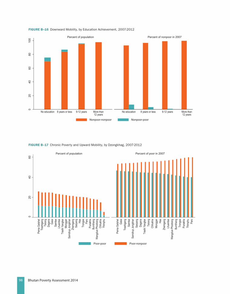
98 Bhutan Poverty Assessment 2014
FIguRE B–16 Downward Mobility, by Education Achievement, 2007-2012
Percent of population
Nonpoor-nonpoor Nonpoor-poor
Percent of nonpoor in 2007
FIguRE B–17 Chronic Poverty and Upward Mobility, by Dzongkhag, 2007-2012
020
4060
Pema
Gats
hel
Tras
higan
gTs
irang
Daga
naGa
saSa
mtse
Lhue
ntse
Tras
hi Ya
ngtse
Mong
gar
Samd
rup J
ongk
har
Zhem
gang
Sarp
ang
Haa
Tron
gsa
Paro
Puna
kha
Bumt
hang
Wan
gdue
Pho
dran
gCh
hukh
aTh
imph
u
Percent of population
Poor-poor Poor-nonpoor
Pema
Gats
hel
Gasa
Tras
higan
gSa
mtse
Samd
rup J
ongk
har
Sarp
ang
Daga
naTr
ashi
Yang
tseTs
irang
Chhu
kha
Mong
gar
Haa
Zhem
gang
Lhue
ntse
Wan
gdue
Pho
dran
gBu
mtha
ngTr
ongs
aPu
nakh
aTh
imph
uPa
ro
Percent of poor in 2007
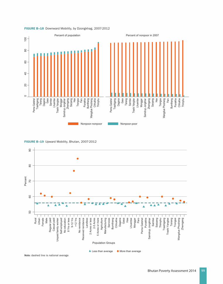
99Bhutan Poverty Assessment 2014
FIguRE B–18 Downward Mobility, by Dzongkhag, 2007-20120
2040
6080
100
Pema
Gats
hel
Tras
higan
gTs
irang
Daga
naGa
saSa
mtse
Lhue
ntse
Tras
hi Ya
ngtse
Mong
gar
Samd
rup J
ongk
har
Zhem
gang
Sarp
ang
Haa
Tron
gsa
Paro
Puna
kha
Bumt
hang
Wan
gdue
Pho
dran
gCh
hukh
aTh
imph
u
Percent of population
Nonpoor-nonpoor Nonpoor-poor
Pema
Gats
hel
Tras
higan
gDa
gana
Gasa
Tsira
ngSa
mtse
Tras
hi Ya
ngtse
Lhue
ntse
Mong
gar
Samd
rup J
ongk
har
Zhem
gang
Sarp
ang
Haa
Tron
gsa
Wan
gdue
Pho
dran
gPa
roBu
mtha
ngPu
nakh
aCh
hukh
aTh
imph
u
Percent of nonpoor in 2007
FIguRE B–19 Upward Mobility, Bhutan, 2007-2012
5060
7080
90
Population Groups
Urb
anR
ural
Fem
ale
Mal
eR
egul
ar p
aid
Cas
ual p
aid
Unp
aid
fam
ily w
orke
rS
elf-e
mpl
oyed
No
educ
atio
n8
Yrs
or l
ess
9-12
Yrs
>12
Yrs
No
rem
itanc
eR
ecei
ved
rem
itanc
eLa
ndle
ss2
Acr
es o
r les
s2-
5 A
cres
5 A
cres
or m
ore
Agr
icul
ture
Man
ufac
turin
gS
ervi
ces
Bum
than
gC
hhuk
haD
agan
aG
asa
Haa
Lhue
ntse
Mon
ggar
Par
oP
ema
Gat
shel
Pun
akha
Sam
drup
Jon
gkha
rS
amts
eS
arpa
ngTh
imph
uTr
ashi
gang
Tras
hi Y
angt
seTs
irang
Tron
gsa
Wan
gdue
Pho
dran
gZh
emga
ng
Less than average More than average
Per
cent
Note: dashed line is national average
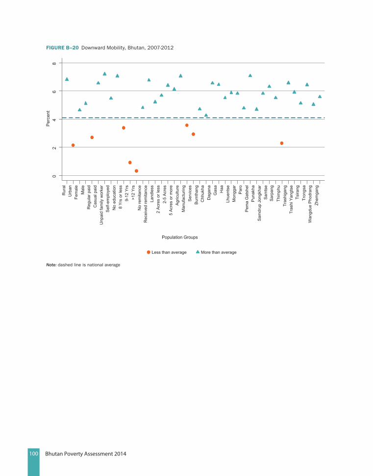
100 Bhutan Poverty Assessment 2014
FIguRE B–20 Downward Mobility, Bhutan, 2007-2012
Urb
anR
ural
Fem
ale
Mal
eR
egul
ar p
aid
Cas
ual p
aid
Unp
aid
fam
ily w
orke
rS
elf-e
mpl
oyed
No
educ
atio
n8
Yrs
or l
ess
9-12
Yrs
>12
Yrs
No
rem
itanc
eR
ecei
ved
rem
itanc
eLa
ndle
ss2
Acr
es o
r les
s2-
5 A
cres
5 A
cres
or m
ore
Agr
icul
ture
Man
ufac
turin
gS
ervi
ces
Bum
than
gC
hhuk
haD
agan
aG
asa
Haa
Lhue
ntse
Mon
ggar
Par
oP
ema
Gat
shel
Pun
akha
Sam
drup
Jon
gkha
rS
amts
eS
arpa
ngTh
imph
uTr
ashi
gang
Tras
hi Y
angt
seTs
irang
Tron
gsa
Wan
gdue
Pho
dran
gZh
emga
ng
02
46
8
Population Groups
Less than average More than average
Per
cent
Note: dashed line is national average
101Bhutan Poverty Assessment 2014
Annex C: Qualitative assessment of Poverty
Introduction
The Bhutan Poverty Analysis 2012 Report shows that living standards continue to improve in Bhutan, with the percentage of people below the official poverty line falling from 23.2 percent in 2007 to 12 percent in 2012. However, while Bhutan overall has made tremendous progress in poverty reduction, especially in reducing rural poverty, some dzongkhags continue in poverty or have a harder time reducing poverty. The drivers of this rapid poverty reduction, and the reasons why some regions remain mired in poverty, are not generally well-understood. In addition to desk-based quantitative research, a qualitative approach is necessary to understand the problems.
This annex presents the findings from 13 focus group discussions (FGDs) organized in four dzongkhags of Bhutan during January and February 2014. The four dzongkhags are Dagana, Zhemgang, Pema Gatshel, and Lhuentse. The findings from these discussions complement the desk-based quantitative research in order to deepen the understanding of poverty dynamics in Bhutan.
Focus Group approaches and methods
For the purpose of the focus group discussions, the four dzongkhags were selected based using the 2012 Bhutan Poverty Analysis Report. In each of the dzongkhags two communities were identified and these were represented by as near to equal numbers of men and women as possible. A gewog (which serves as the administrative center for a group of villages, or chiwogs) was therefore taken as a “community”. The dzongkhag administration, dzongkhag planning officers, respective dzongkhag
administrators, and Dzongkhag Statistical Officers (DSOs) were consulted and relevant poverty documents used to select the most suitable gewogs. The selected gewogs for each dzongkhag are presented in Table C–1.
Separate focus group discussions were con-ducted for men and women in each selected community, where possible, although some groups comprised both genders. The reason for separating the men and women was mainly to provide the women with an enabling environ-ment to more candidly share their opinions on issues of poverty and wellbeing from a gender perspective.
To the extent possible, participants for the focus groups were selected from poor households and non-poor households. The poor households comprised participants with small land holdings, some were agriculturists, or derived livelihoods from nonfarm activities, and some were women heads of households. Participants for the better-off households were shopkeepers, cash-crop owners, non-poor farmers, small businessmen, contractors, etc. In-depth insights into the communities were also obtained through interviews with the key informants, including local leaders such as gewog heads (gups), sector heads in the community such as the Renewable
TABlE C–1 Gewogs and Dzonkhags Selected for Focus Group Discussions
Dzongkhag gewog
Dagana Kana and Drujeygang
Zhemgang Nangkhor and Phangkhar
Pema Gatshel Shumar and Khar
Lhuentse Gangzur and Metsho
102 Bhutan Poverty Assessment 2014
Natural Resource (RNR) extension agents (of the Agriculture Ministry), health workers, and local committees such as village women’s groups, vegetable groups, and interviews with the elderly from the community typically known as the “Go-Shey Nyen-Shey”.
A similar format for the questions was used in order to obtain a standardized to set of responses so as to understand the various communities’ perceptions of poverty, the strengths of the communities, factors hindering or helping com-munity prosperity at the community level, and improvements or declines in income at household level. The specific questions are:
In your context what do you think of poverty?
Community LevelLet us talk about your community. What is going well here?
In the last five years what do you think about the community? Is it
• More prosperous?• Remained the same?• Less prosperous?
Household Level
Do you think that your income increased in the last five years? Yes or No.
All discussions were recorded and notes were taken simultaneously. A paired wise ranking matrix was used for the community level discussions to list down and identify the top three community prosperity or declining factors through a consensus-building approach. Summary findings and detailed findings from the discussions are presented below.
summary of Key Findings
Community perspective on poverty: Focus group participants generally perceived poverty
as deprivation12 of basic necessities required for a decent living. For most of them basic necessities meant having sufficient food to eat, water accessibility, and a house to live in. Deprivation of these necessities affected the wellbeing and likelihood of a household’s vulnerability to poverty. For most of the participants whose livelihood system was dependent on cash crops, poverty was about risk and vulnerability to pests and diseases, natural disasters such as drought, irrigation constraints, and human-wildlife conflict. The situation was further constrained by the fact that communities lacked concrete solutions to the problems and absence of coping mechanisms and strategies to offset the losses which directly affected their wellbeing.
Primary indicators of poverty identified by the participants:“Insufficient food to eat. We just work to eat”.“Not having an income earning source”.“Lack of Income”.“Children not able to eat”.“No proper house to live in”. “Living in a bago (bamboo hut)”.“Not having land”.
Women’s Perspective on Poverty: Women generally perceived poverty as lacking money, having insufficient food to eat and drink, and no proper house to live in. A few participants considered money a key criterion to differenti-ate between rich and poor. For some, having no endowments such as land, being a sharecropper and relying on other’s land for livelihood is what poverty about. Similarly, for some households poverty is when members of the households, including children, do not have sufficient food to eat and parents are not able to afford higher education for their children. Poverty is about old age, lack of employment, with elderly left behind in the villages unable to do hard labour, thereby
12 Scarcity and not necessarily denial
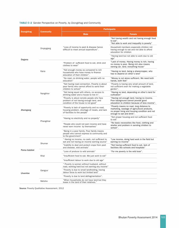
103Bhutan Poverty Assessment 2014
TABlE C–2 Gender Perspective on Poverty, by Dzongkhag and Community
Dzongkhag CommunityParticipants
Male Female
Dagana
Drujeygang “Loss of income to pest & disease hence difficult to meet annual expenditure”.
“Not having wealth and not having enough food to eat”. “Not able to work and inequality is poverty”
Household members especially children not having enough to eat and not able to afford education for children
“Having land but not able to work due to old age”
Kana
“Problem of sufficient food to eat, drink and clothes to wear”
“Lack of money. Having money is rich, having no money is poor. Being rich also means owning car, land, everything house”
“Not enough money as compared to rich households who have money to finance education of their children”.
“Having no land, being a sharecropper, who has to depend on other’s land”
“No road, no drinking water, people with no education”
“Money is not alone sufficient. We need both hands, both feet”
Zhemgang
Nangkhor
“Not having road connection. Poverty is about poor family who cannot afford to send their children to school”
“Poverty is having very small amount of land, not sufficient even for making a vegetable garden”.
“Not being equal with others, no access to drinking water and a house to live in”.
“Having no land, depending on other’s land for cultivation”
“Poverty is about remote people who face problem of not having enough land, and condition of the house is not good”
“Having not enough land, having no income. Poor background cannot provide good education to children because of less income”.
Phangkhar
“Poverty is lack of opportunity and no road, housing problem, shortage of meals, and lack of facilities to the people”
“Poverty means no road, long distance to marketing, wastage of agricultural products, no proper living and housing condition and not enough to eat and drink”.
“Having no electricity and no property” “Not proper housing and not sufficient food to eat”
“People who could not earn income and have never earn income by themselves”
“No basic necessities like food, clothing and shelter and problem in sending children to school”.
“Being in a poor family. Poor family means people who cannot express to community and to the government”
Pema Gatshel
Shumar
“ Having no income, no cash, not sufficient to eat and not having an income earning source”
“Low income, doing hard work in the field but earning no income”
“Inability to deal and protect crops from pest and disease, wild animals”
“Not having sufficient food to eat, lack of facilities like schools and hospitals”
Khar
“Loss of produce to wild animals” “For me poverty is the wild boar”.
“Insufficient food to eat. We just work to eat”
“Insufficient labour to work due to old age”
LhuentseGangzur
“ Poverty is women without husband, without road, working hard but not earning any income”
“Poverty is due to small landholding, having labour force to work but limited land”
“Poverty is due to land defragmentation”.
Metsho “When households do not have land but they lease in the land of their relatives.”
source: Poverty Qualitative Assessment, 2012

104 Bhutan Poverty Assessment 2014
age directly harming their livelihood. Women also perceived poverty as isolation caused by re-moteness, lack of accessibility to markets, and lack of health and educational opportunities.
Men’s Perspective on Poverty: Men’s perception of poverty tend to converge with those of women in terms of limitation of income, deprivation of basic necessities for a decent living in addition to remoteness, lack of road network, lack of electricity, health and educational facilities. More precisely men identified poverty as being in a poor family and constrained by the household’s inability to express their plight to the community or the government. Poverty is about people who could not earn income and never have earned income by themselves. When discussing poverty, men spoke of it as the destruction of the principal income-earning source, such as oranges and cardamom by pests and diseases and lack of knowledge to cope with such disasters. Some participants identified poverty as not having wealth, having only small land holdings, and female-headed households with no male members to work.
Livelihood Resources: The livelihood portfolio in the study area is diverse and most commu-nities identify subsistence agriculture, land, livestock, cash crops, industries, organic farm-ing and employment in nonfarm sectors as their livelihood resources. Subsistence agriculture characterized by labour-intensive traditional methods of farming is common in all the com-munities. Livelihood for community in Dagana is predominantly dependent on cash crops such as oranges and cardamom which are exported to India. In addition communities also grow maize and vegetables such as beans, cabbages, cauliflower for self-consumption. Communities in Nangkhor in Zhemgang grow rice although the area is also suitable for cardamom and sup-port organic farming. In lower regions of the dzongkhag such as in Phangkhar maize is the
principal food crop in addition to community’s popularity for oranges. In Pema Gatshel maize is widely grown but orange is the main cash crop. The community is also very rich in mineral resources such as gypsum. Lhuentse is charac-terized by rugged terrain and land endowments are restricted to small holdings and subsistence agriculture is predominant. Most of the commu-nities under study have access to basic facilities such as road network, power supply, mobile con-nectivity, a Basic Health Unit (BHU), a school and access to Renewable Natural Resources (RNR) and livestock extension services.
Factors Affecting Community Prosperity: Despite the community’s richness in natural resources and endowments majority of the FGD participants identified factors which they considered was hindering the community prosperity. These factors included lack of irrigation, vulnerability of crops to pest and diseases, market in-accessibility, small landholding, human wild life conflict, absence of road networks, lack of access to rural credit, lack of labour force, declining social capital and cohesion, impact of mining industry, lack of school, and rural to urban migration. These factors have significantly affected the community in different ways. During each of the focus group discussion factors identified by the participants were listed and a paired wise ranking matrix was used through a consensus building approach to identify the top three factors specific to and affecting the community.
In Dagana vulnerability of cash crops to pest and diseases have affected the annual income of the community. Market inaccessibility due to longer distance to the market, poor quality of farm road and inaccessibility throughout the year was limiting opportunities for farmers to exploit the benefit of organic farming. Drought and drying of natural streams and human wild life conflict have also significantly affected this community.
105Bhutan Poverty Assessment 2014
In Nangkhor community of Zhemgang irrigation constraints, market inaccessibility and small land holding were the top three factors affecting the community experience with prosperity. Women had a somewhat different view. For them it was the small land holding, lack of irrigation and poor transport infrastructure (road) affecting the community. Similar problems of drying streams were reported forcing farmers to increasingly depend on monsoon hence labour intensive farming was impossible for households who lacked enough labour force. Market inaccessibility was as a result of poor road network (farm roads), longer distance to the domestic market and often problem in economies of scale in production due to smaller land holding.
Community from Phangkhar in lower Zhemgang identified absence of road network, limited higher educational facilities and vulnerability to wild life as the principal factors. Women identified lack of credit facilities limiting entrepreneurial opportunities in addition to absence of road network and educational facilities.
In Pema Gatshel both the communities from Shumar and Khar identified similar factors affecting the community experience with prosperity. These included vulnerability of high valued cash crops to pest and diseases, lack of irrigation, and human wild life conflict. The difference was, for the Khar community labour shortage was impacting them the most as compared to wild animals attacking crops for the Shumar community. However women participants from Shumar community identified two new factors including the negative impact of mining and limited access to credit in addition to pest and disease affecting the cash crops as the top three factors.
In Pema Gatshel gypsum is one of the main natural resources where mineral is extracted and exported to India. Majority of the participants both men and women observed that mining
provided little or no benefits to the community. Employment opportunities for the local community were limited, constrained by the lack of skills of the local people in operating heavy equipment. The community observed that the dust, pollution and frequent explosions in the mining site was damaging their crops, and affecting water scarcity. In Lhuentse both the communities identified small land holding, market inaccessibility and lack of irrigation although there were differences in the ranking of these factors.
Across the four dzongkhags and the communities most of these factors frequently featured during the discussion in both the groups disaggregated by gender. The most common factors identified were:
1. Lack of Irrigation2. Pest and diseases affecting the cash crops
(oranges and cardamom)3. Market inaccessibility and Small Land
Holding4. Human wild life conflict5. No road network &no education facilities
and limited access to credit6. Impact of mining & labour shortage &
poor infrastructure (road)Poverty and Household Wellbeing: At the
household level participants both men and women generally believed that their income improved now as compared in the past. This was possible because household members could now diversify their sources of income through nonfarm activities by working as daily wage workers, as small contractors and selling livestock products and vegetables in small quantities to public servants at the gewog centers.
Majority of the participants also observed that daily wages for both skilled and unskilled workers have increased with increase in demand for such workers. Some of the emerging issues affecting the households were use and abuse
106 Bhutan Poverty Assessment 2014
of alcohol, limited social cohesion, lack of self-help groups and increasing trends in divorce. Such emerging issues at times shifted the entire burden of raising family including children on women. Female headed households with no male members also found it challenging to exchange labour in the neighborhood because of preference and expectations of reciprocal arrangements of labour contributed by a male workforce.
Factors Affecting Community Prosperity: The focus group participants identified the strengths of their own community in terms of factor endowments such as land, fertile soil, favorable climatic conditions, production and trade in high value cash crops like oranges and cardamom, and developments in physical infrastructure. Participants recognized that investment in physical infrastructure by the government like development of road networks including farm roads construction, provision of electricity, mobile connectivity, and access to drinking water have improved their living conditions as well helped them diversify their income earning opportunities/portfolios.
These developments over the last five years enhanced improvements in people’s lives as households observed a rise in income, facilitated easier access to public services, increased access to health and educational facilities, access to essential goods and services, RNR support services amongst others. However, despite the community richness in the factor endowments and the developments in physical infrastructure and improved accessibility participants expressed their inability in having fully exploited the endowments which otherwise would have helped them enhance their livelihood. The focus group participants identified range of factors which according to them was hindering community prosperity. By using a paired wise ranking matrix through consensus building approach a list of top three factors hindering the
community prosperity were identified which is presented in Table1.
Common Factors affecting Community
ProsperitySome common factors derived from Table C–1
affecting the community prosperity were identi-fied based on the number of times it occurred as shown in Table C–2. Across the 13 focus groups, lack of irrigation significantly affected communi-ty prosperity cutting across men and women. Pest and diseases affecting the cash crops came as the next important factor followed by market inac-cessibility & small land holding. While all factors were common across men and women, limited access to credit was one factor women raised as a hindrance to community prosperity. Human wild life conflict is of course a pervasive problem across all the communities but it did not strongly feature in the list of top three factors across all communities, men and women.
The dzongkhag and community-wise presentation of top three factors affecting community experience with prosperity showed male participants in Dagana identifying pest and diseases affecting their cash crops, market inaccessibility, and irrigation constraints. Women participants identified human wild life conflict as the third factor affecting the community prosperity in addition to irrigation constraints, pest and diseases affecting the cash crops. The preference for market inaccessibility was the least for the women group.
For the male communities of Nangkhor gewog under Zhemgang dzongkhag, irrigation constraints, market inaccessibility and having small land holding were the top three factors affecting the community mobility. Women had a somewhat different view. For them it was the small land holding, lack of irrigation and poor transport infrastructure (road) affecting the community wellbeing. Similarly male
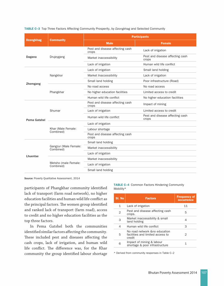
107Bhutan Poverty Assessment 2014
participants of Phangkhar community identified lack of transport (farm road network), no higher education facilities and human wild life conflict as the principal factors. The women group identified and ranked lack of transport (farm road), access to credit and no higher education facilities as the top three factors.
In Pema Gatshel both the communities identified similar factors affecting the community. These included pest and diseases affecting the cash crops, lack of irrigation, and human wild life conflict. The difference was, for the Khar community the group identified labour shortage
TABlE C–3 Top Three Factors Affecting Community Prosperity, by Dzongkhag and Selected Community
Dzongkhag CommunityParticipants
Male Female
Dagana Drujeygang
Pest and disease affecting cash crops Lack of irrigation
Market inaccessibility Pest and disease affecting cash crops
Lack of irrigation Human wild life conflict
Zhemgang
Nangkhor
Lack of irrigation Small land holding
Market Inaccessibility Lack of irrigation
Small land holding Poor infrastructure (Road)
Phangkhar
No road access No road access
No higher education facilities Limited access to credit
Human wild life conflict No higher education facilities
Pema Gatshel
Shumar
Pest and disease affecting cash crops Impact of mining
Lack of irrigation Limited access to credit
Human wild life conflict Pest and disease affecting cash crops
Khar (Male Female: Combined)
Lack of irrigation
Labour shortage
Pest and disease affecting cash crops
Lhuentse
Gangzur (Male Female: Combined)
Small land holding
Market inaccessibility
Lack of irrigation
Metsho (male Female: Combined)
Market inaccessibility
Lack of irrigation
Small land holding
source: Poverty Qualitative Assessment, 2014
TABlE C–4 Common Factors Hindering Community Mobility*
Sl. No Factors Frequency of occurrence
1 Lack of irrigation 11
2 Pest and disease affecting cash crops. 5
3 Market inaccessibility & small land holding 4
4 Human wild life conflict 3
5No road network &no education facilities and limited access to credit
2
6 Impact of mining & labour shortage & poor infrastructure 1
* Derived from community responses in Table C–2
108 Bhutan Poverty Assessment 2014
impacting them the most as much as wild animals attacking crops for the Shumar community. However women from Shumar community identified two new factors including the negative impact of mining and limited access to credit in addition to pest and disease affecting the cash crops as the top three factors. In Lhuentse both the communities identified similar factors such as small land holding, market inaccessibility and lack of irrigation although there were differences in the ranking of these factors.
Besides the top three factors hindering the community prosperity the most, there were factors which emerged strongly during the discussion but did not feature in list of three factors during the consensus building process. Some of these factors include, rural to urban migration, declining conditions of social capital and cohesion, lack of self-help groups, use and abuse of alcohol, natural disasters, increasing trend in divorce cases etc. The impact of top three factors and the emerging issues affecting the community prosperity are discussed in detail below under economic, social and environmental factors.
economic Factors
Loss of Income to Pests and Diseases: The dzongkhags of Dagana, Pema Gatshel and Zhemgang are located in the southern belts of the country. The sub-tropical climatic conditions and soil quality make the dzongkhags suitable for growing cash crops like oranges and cardamom. Most commonly the lower regions of the dzongkhags are popular for producing oranges while in the higher altitudes of Dagana cardamom is also grown. For the people of Dagana cardamom and oranges are therefore the two main sources of income, compared to mainly oranges for the communities of Pema Gatshel and Zhemgang. The livelihood of these communities is dependent on the annual income from the sale of cash crops. Households use the annual income in meeting the
basic needs, buying of essential items, meeting the educational expenses of their children, and even financing of higher education of their children amongst others.
In Dagana participants from both the communities reported loss of the cash crops to pest and diseases. This has reduced the total yield and subsequently affected the total annual income of the households. The communities also lacked coping strategies to offset the loss of income from pest and disease although some households reported having shifted to pulses (dal) farming which they export to buyers in India.
In Zhemgang the pest and disease severely affecting the cash crops was however not reported. In Pema Gatshel both the communities mentioned pest and disease having affected their cash crop and hence the income. Men ranked it as the top factor while women ranked it as the third factor affecting their livelihood. Both male and female participants believe that dust from the gypsum mine responsible for causing damage to the cash crop.
Market Inaccessibility: Participants perceive increasing and potential opportunities in organic farming to supplement cash income when their principal income sources have been affected by pest and diseases and irrigation constraints have affected agriculture. They also immediately recognize the absence of a market generally characterized by limited buyers. The community’s understanding of a market also remotely extend beyond the local market such as the nearest town, the dzongkhag headquarters and to the extent possible the national market such as Thimphu and border towns of Phuentsholing, Gelephu, and Samdrup Jongkhar. Communities have limited knowledge of export markets such as India although they recognize lack of competitiveness of their products as a result of cheaper alternatives available from India. Participants recognized both external and internal factors

109Bhutan Poverty Assessment 2014
rendering market inaccessible. Factors such as longer distance to a potential market, poor quality of the road, high cost of transportation, and absence of marketing infrastructure, and cheaper alternatives were external and beyond
the control of the community. The community also lacked production, marketing, packaging and handling skills as internal constraints resulting in non-competitiveness of the products.
Small Land Holding: Participants from the
“We even tried producing and selling local vegetables however potential buyers lack interest in our vegetables because they say that our vegetables lack quality even though we think that our prices are reasonable selling a Kg of Cabbage at Nu20 and a bundle of broccoli at Nu 50. For example I and my friend hired a Bolero pickup truck paying Nu 4,000 as transport charges in delivering our vegetables including broccoli and cabbage to Punakha but could not sell because buyers and customers were not interested in our products” – A male FGD participant from Drujeygang gewog.
“The income from the oranges has gone down from average Nu 50,000 to Nu 20,000 so we do not know what to do next. May be we should plant mountain hazelnut as an alternative. Heard that a weather condition of our area is similar to that of Lingmithang in Monggar and it might work here” – A male FGD participant, Shumar Pema Gatshel
“Many orange orchards are damaged by disease these days. Now oranges are not even available to eat. First it affected the trees in Denchi village and shifted upwards. Many people of our locality believe that dust from Gypsum powder factory leads to dying of the crops as well as orange” – A female FGD participant, Shumar Pema Gatshel
“I didn’t see the insect but the root of the orange tree has been damaged”– A female FGD participant, Shumar, Pema Gatshel.
“According to the agriculture sector the solution to the disease, is after many rounds of discussion, we have been advised to cut down all the orange trees even if all the trees in the orchard are not affected. If even one tree is affected rest of the trees also has to be cut down and burnt. The government is providing free orange saplings. Now farmers are apprehensive to the advice because the question is how they would manage without income until the new trees start bearing fruits. It takes at least five years to start bearing fruits”– A key informant, Shumar, Pema Gatshel

110 Bhutan Poverty Assessment 2014
Nangkhor community in Zhemgang pointed out their constraints to economies of scale in production due to small land holding. Otherwise they acknowledge the favorable climatic conditions, soil fertility for growing different types of vegetables, and cash crops like cardamom. Small land holding is also the consequence of land defragmentation because of divisions among family members. Female participants defined poverty in relation to small landholding not even sufficient for a vegetable garden and depend on others land for cultivation. In Lhuentse both the communities pointed out the implications of small landholdings limiting opportunities to access credit from formal financial institutions like the Bhutan Development Bank Ltd. (BDBL). The
formal financial institutions require immovable property such as a land or a house as collaterals while extending credit facilities in absence of micro finance institutions. The participants feel that small land holding and inflexible credit requirements limit innovations, entrepreneurial opportunities with lack of economies of scale in production. Small land holding is also the outcome of land defragmentation as a result of land division among family members.
Limited credit facilities: Due to the seasonality of agriculture production and downturn in the production of cash crops communities greatly recognize the importance of working capital and consumption credit. The difficulty in accessing credit facilities in the rural areas limit business opportunities for young entrepreneurs, small
“We do not have sufficient land. Small landholding is a problem. Why because of distributing the land to the children resulting in land getting smaller and smaller due to division/defragmentation” A male FGD participant, Gangzur community.
“Getting loan is also a problem because collaterals are required. Suppose if we think we can get some loan to buy livestock (pig) and earn some income it is not possible. We are asked if we have land or not. When we say no we do not have land, then we are told that we would not be eligible for the loan. In place like Thimphu it would be easy to get loan simply by mortgaging a building and can make profit from it” – A male FGD participant, Gangzur community.
“Our vegetables are not competitive against the one imported from border town of India because it is said that our cabbages contains lot of water inside, the cabbages are not green, the leaves are yellowish and due to poor quality of road vegetables get damaged while transporting them to longer distance” – A male FGD participant, Drujeygang gewog.
“Although we have now, electricity, road but the prices in the market have increased. Things are very expensive. We do not have a market to sell our products like vegetables. People are far off from the market in the cliffs. We do not have even place to keep tourist. They all return to Monggar” – A male FGD participant, Gangzur community, Lhuentse
111Bhutan Poverty Assessment 2014
contractors in diversifying their economic activities. Formal financial institutions have collateral requirements which make it not feasible for the farmers to access loan in absence of specific collaterals demanded by the bank. It is not lack of collaterals. In fact farmers have specific collaterals such as small land holding, labour, but which are not acceptable to the bank. Limited access to credit was one of the reasons cited by women group of Phangkhar community in Zhemgang. According to the participants men earn income from different sources such as construction works, as daily wage earners working in the road side and engage in other nonfarm activity. In contrast women sources of income is limited to daily wages from carrying oranges. Since the community do not have access to road woman carry oranges from villages until the highway and is the only source for them once a year during the harvest season.
In the remaining part of the year women mend their fields. Since the orange yield has been affected by pest and disease their income has also been affected. Women see potential opportunities through self-employment. Young women also have been trained in tailoring, hair dressing, beauticians, etc. through government’s rural poverty reduction strategies but credit facilities is a big constraint for them.
Labour shortage (Labour as input & number of labourers): Community understanding of labour shortage differed according to the situation affecting the labour intensive agriculture sector. For some community it is the decreasing input as labour because of old age since young people have migrated to urban centers leaving the elderly behind. In comparison Nangkhor community in Zhemgang believed limited work force in the households affecting the labour as input affecting their livelihood because the community is entirely dependent on monsoon for transplanting rice. During monsoon transplanting coincides across
households and exchange of labour is impossible. Sometime households with fewer labour forces cannot carry out the transplantation leaving the land fallow.
social Factors
The community understanding of poverty was not limited to income alone. Some of the factors that emerged during the discussion were social in nature. A factor such as lack of accessibility to market was due to poor road infrastructure and absence of road network in some community. A community in Zhemgang pointed out lack of higher educational facilities in the community affecting their livelihood because a huge amount of recurring expenditure was incurred on children in arranging education facilities outside the community.
“We also request for farming machineries because of water scarcity we depend on monsoon rain to transplant paddy. When there is monsoon everyone in the village start transplanting paddy and therefore we cannot exchange labour and sometimes we have to keep our land fallow” – A male FGD participant, Nangkhor Community
“During summer we face problems of paddy transplantation as the water on irrigation channel dries on the way to our fields and we have to depend on the monsoon and every households start planting when it starts raining so we face labour shortage” – A male FGD participant, Nangkhor Community
112 Bhutan Poverty Assessment 2014
Some of the emerging social issues identified by the participants were use and abuse of alcohol, increasing trend in divorce, limited number of self-help groups, lack of social capital and social cohesion and rural to urban migration. The abuse of alcohol is mostly associated with men. According to some women participants a considerable income is spent on buying alcohol which is easily available in the market. It not only impacts the income but also affects the household wellbeing because participants think that alcohol is also associated with increasing trend in divorce and other social problems. Divorce and alcohol related challenges are pervasive in nature and present in most of the communities. There is a general agreement that social capital and cohesion among communities is slowly degenerating. The existence of informal network is very helpful but it demands reciprocal treatment. Women headed households are vulnerable to poverty because reciprocal arrangements are expected for male labour contribution.
When discussing rural to urban migration participants pointed out absence of permanent migration in large numbers. Of course few households in the community have migrated to urban centers accompanying their children. Rural to urban migration according to the community is mostly common among educated youths who move to urban centers in search of better opportunities. It is therefore not on account of surplus labour generated by the agriculture sector. The agriculture sector is unattractive to youths and labour shortage continues to be a constraint for the sector with mostly elderly labour force staying behind.
environmental Factors
Irrigation Shortage: Lack of irrigation is discussed under this section because most communities attributed the problem to
“One of the main problems is that we are not able to protect our crop from wild animals such as wild boars and monkeys. On top of that important cash crops like oranges and cardamom have been affected by diseases and their yield have declined over the years. These problems have also resulted some of the households to migrate to urban areas. When one household migrates other households also think of migrating and the area and the farm of the migrated household when not maintained it turns into thick jungle making it easier for wild animals to attack crops in the locality” – A male FGD participant, Kana Community, Dagana
“I also feel that we do not have educated people remaining in the community because they all are in the urban centers employed in some sectors or doing some business”. – A male FGD participant, Kana Community, Dagana
“In my opinion if we have access to better extension services (marketing) access to credit, provision of seeds, hybrid cattle, provision of cattle feed, pesticides, enough water for irrigating our vegetable garden would solve most of the problem” – A female FGD participant, Kana gewog

113Bhutan Poverty Assessment 2014
environmental destruction, climate change, and drought. Irrigation emerged as principal factor affecting all most all the communities in the four dzongkhags. In Lhuentse and Pema Gatshel irrigation shortage has affected both domestic consumptions as well as affected farming. While for the Nangkhor community in Zhemgang the shortage has mostly affected farming.
Irrigation shortage has also linkages with the dying of the cash crops in Dagana and Pema Gatshel because firstly these cash crops require irrigation in absence of rain. Secondly organic farming is the only alternative for communities to offset the loss of income to pest and dis-eases. In Nangkhor, the drying of the streams has left farmers to depend on rain. In absence of timely rainfall and lack of labour force wet lands have remained fallow. In Pema Gatshel too, drying of streams have rendered some 30 acres of paddy field fallow. The unique prob-lem in Pema Gatshel is that the streams are frequently shifting their locations downwards every year and households located in higher al-titude have water scarcity.
Vulnerability and Risks: Crop losses due to pest and diseases, and wild life and natural di-sasters like storms, earthquake and drought make the community vulnerable to poverty. The principal risks in agriculture across all the com-munity was identified as wild life attacking both food and cash crops. Farmers are left to harvest sometimes only the remnants of the crops. The community believes that increasing conflict is as a result of human encroachment due to de-forestation, construction of roads, erecting of electricity poles and other developmental activi-ties. Farmers have no access to compensation for the damage given the challenges in assessing the extent of the damage caused and in absence of crop insurance.
Concluding observations
The findings of the focus group discussion present similarities in patterns of factors hindering the community prosperity. Lack of irrigation, vulnerability of principal crops to pest and diseases, market inaccessibility and loss of crops to wild animals amongst others were perceived as important conditions of community wise experience with decline. The findings suggest that these common factors are often external in
“We have only a primary school that was established some 30 years ago. Upgrading of the schools will have benefits such as we can sell some of our local produce and we do not have to send our children to school which is very far. It incurs huge additional cost in transport, living arrangements, frequent buying of school uniforms, shoes when we have to send our children to other schools. If we do not have to change schools so frequently school uniforms, shoes last for many years and children can stay with us and attend classes” – A male FGD participant, Phangkhar community, Zhemgang.
“There is no up gradation of the school in the Gewog due to which we have to send our children to other far off school. We face financial problems. The BHU also has male health assistant. We women face problem in discussing our health issues” – A female FGD participant, Phangkhar community, Zhemgang.

114 Bhutan Poverty Assessment 2014
nature and beyond the control of the community who are less endowed with technical knowledge and expertise in immediately solving the problems by themselves.
Problems of irrigation and drought show community’s vulnerability and limited resilience to the forces of climate change although the country has abundant fast flowing rivers but beyond the rich of these specific communities. The cash crops vulnerability to pest and diseases demands a better understanding of the causes and requires a long-term solution that is also acceptable to the community. Possible and
immediate solutions may be, sharing of best practices, lesson learning experiences and exploring and diversifying alternative livelihood strategies.
There are also opportunities for improving the community livelihood. Most of the community have the required infrastructure in place such as road, electricity, mobile services access to health and educational facilities. The agriculture extension services provided by the RNR sector in provision of seeds, fertilizers, and technical skills in marketing of organic products are significant.
“For this community maize has been principal food from time immemorial. People use to grow maize and eat as a special diet to work in the fields but due to drought we could not harvest like before which has affected our food security” – A male FGD participant, Drujeygang, Dagana
“We have lot of wet land for paddy cultivation but now the water sources have started drying up and there is limited volume of water left for sharing among households. Lack of irrigation channel is a problem on top of that due to which wet land remains fallow” – A female FGD participant, Drujeygang, Dagana
“Nowadays we have been experiencing hot weather with rise in temperature and may be this is because of lot of constructions works going on and building of factories elsewhere which causes pollution. Water sources have been drying up because may be we are using excessive wood for construction of houses and blasting. Even the taste of oranges is not that sweet like before may be because of the heat”– A female FGD participant, Drujeygang, Dagana
“The dust from the mining might have affected the oranges. Drinking water was really not a problem but may be because of the dust and the bombings the source of drinking water is shifting downwards. Dust has affected the trees, animal fodder and because of no rain dust does not settle”– A male FGD participant, Shumar community Pema Gatshel
115Bhutan Poverty Assessment 2014
RefeRences
Alkire, S. 2011. “A National MPI for Bhutan: Three Trial Measures.” Oxford Poverty and Human Development Initiatives, Oxford.
Atkinson, A.B. 1987. “On the Measurement of Poverty.”Econometrica, Vol. 55, No.4: 749-764.
Benjamin, Dwayne, Loren Brandt, and John Giles. 2005.“The Evolution of Income Inequality in Rural China.”Economic Development and Cultural Change, Vol. 53, No.4: 769-824.
Bhutan Multiple Indicator Survey. 2010. National Statistics Bureau, Royal Government of Bhutan.
Bourguignon, François, Francisco H. G. Ferreira, and Nora Lustig. 2005. Introduction in François Bourguignon, Francisco H.G. Ferreira and Nora Lustig (eds), “The Microeconomics of Income Distribution Dynamics in East Asia and Latin America,” pp. 17-46, Washington, D.C.: The World Bank.
Dang, H-A. and P. Lanjouw. 2013. “Measuring Poverty Dynamics with Synthetic Panels Based on Cross-Sections.” World Bank Policy Research Paper number 6504, Washington, DC.: World Bank.
Datt, Gaurav, and Martin Ravallion. 1992.“Growth and Redistribution Components of Changes in Poverty Measures: A Decomposition with Applications to Brazil and India in the 1980s.”Journal of Development Economics, 38: 275-95.
Dercon, S., D.O. Gilligan, J. Hoddinott, and T. Woldehanna.2009. “The Impact of Agricultural Extension and Roads on Poverty and Consumption Growth in Fifteen Ethiopian Villages,” American
Journal of Agricultural Economics, 91 (4), 1007–1021.
Duclos, Jean-Yves. 2009. What is “Pro-Poor”?Social Choice and Welfare, 32:37-58.
Essama-Nssah, B. 2012. “Identification of Sources of Variation in Poverty Outcomes.” World Bank Policy Research Working Paper No. 5954. Washington, D.C.: The World Bank.
Essama-Nssah., B. and Peter J. Lambert. 2009.“Measuring Pro-Poorness: A Unifying Approach with New Results.”Review of Income and Wealth, Series 55, No. 3: 752-778.
FAO (Food and Agriculture Organization). 2011. Guidelines for Measuring Household and Individual Dietary Diversity, FAO. Nutrition and Consumer Protection Division, Food and Agriculture Organization of the United Nations, Rome, Italy. Available online at <http://www.fao.org/fileadmin/user_upload/wa_workshop/docs/FAO-guidelines-dietary-diversity2011.pdf>
Firpo, S., N. Fortin, and T. Lemieux. 2009. “Unconditional Quantile Regressions,”Econometrica, 77, 953-973.
Foster, James E., J. Greer, and E. Thorbecke. 2010.“The Foster-Greer-Thorbecke (FGT) Poverty Measures: 25 Years Later.” Journal of Economic Inequality, 8: 491-524.
Gross National Happiness Report. 2010. Gross National Happiness Survey results 2010, Available online at <http://www.grossnationalhappiness.com/survey-results/index/>
Hettige, H. 2006. “When do Rural Roads Benefit the Poor and How? An In-depth
116 Bhutan Poverty Assessment 2014
Analysis Based on Case Studies,” Asian Development Bank, Manila, Philippines.
IMF (International Monetary Fund). 2010a. Bhutan: Poverty Reduction Strategy Paper. IMF Country Report No. 10/180. Washington, D.C.: IMF.
IMF (International Monetary Fund). 2010b. Bhutan: Poverty Reduction Strategy Paper – Joint Staff Advisory Note. IMF Country Report No. 10/181. Washington, D.C.: IMF.
Jenkins, S. and Peter J.Lambert.1997.“Three ‘I’s of Poverty Curves, with Analysis of UK Poverty Trends.” Oxford Economic Papers, 49: 317-327.
Kennedy, G., T.Ballard, and M-C. Dop. 2011. “Guidelines for Measuring Household and Individual Dietary Diversity.” Nutrition and Consumer Protection Division, Food and Agriculture Organization (FAO) of the United Nations, Rome, Italy. Available online at <http://www.fao.org/fileadmin/user_upload/wa_workshop/docs/FAO-guidelines-dietary-diversity2011.pdf>
Khandker, S.R., Z. Bakht, and G. B. Koolwal. 2009. “The Poverty Impact of Rural Roads: Evidence from Bangladesh”, Economic Development and Cultural Change, 57, 685–722.
Kray, Aart. 2006.“When is Growth Pro-Poor? Evidence from a Panel of Countries.” Journal of Development Economics, 80: 198-227.
National Statistics Bureau. 2013. Available<http://www.nsb.gov.bt/publication/publications.php?id=3>
Osmani, S. 2005.“Defining Pro-Poor Growth.” One Pager Number 9, International Poverty Center, Brazil.
PovcalNet: the on-line tool for poverty measurement developed by the
Development Research Group of the World Bank: http://iresearch.worldbank.org/PovcalNet/index.htm?0
Ravallion, Martin. 1994.“Poverty Comparisons.” Chur (Switzerland): Harwood Academic Publishers.
Ravallion, Martin., and Shaohua Chen. 2003.“Measuring Pro-Poor Growth.” Economics Letters 78: 93-99.
RGoB (Royal Government of Bhutan). 2013. Poverty Analysis Report 2012. Thimphu: National Statistics Bureau.
———2007. Poverty Analysis Report 2007. Thimphu: National Statistics Bureau.
Shorrocks, A.F. 1999. “Decomposition Procedure for Distribution Analysis: A Unified Framework Based on Shapely Value”. University of Essex and Institute for Fiscal studies, Colchester, England.
Tiwari, S., E. Skoufias, and M. Sherpa. 2013. “Shorter, Cheaper, Quicker, Better: Linking Measures of HouseholdFood Security to Nutritional Outcomes in Bangladesh, Nepal, Pakistan, Uganda, and Tanzania.”Policy Research Working Paper 6584. Washington, DC.: World Bank.
Ura, K., S.Alkire, T.Zangmo, and W. Wangdi. 2012. “An Extensive Analysis of GNH Index”, Center for Bhutan Studies: Thimphu, Bhutan. Available online at, <http://www.grossnationalhappiness.com>
Warr, P. 2010. “Roads and Poverty in Rural Laos: an Econometric Analysis.”Pacific Economic Review, 15(1), 152-169.
WHO (World Health Organization). 2013. Pro-gress on Sanitation and Drinking Water. Water Supply and Sanitation Monitor-ing, Joint Monitoring Programme for Water Supply and Sanitation, 2013
World Bank. 2010. Sustainable Transport for All: Helping People to Help
117Bhutan Poverty Assessment 2014
Themselves, Rural Transport, IDA at Work in Transportation –2010 Report. Available online at, <http://siteresources.worldbank.org/IDA/Resources/73153-1285271432420/IDA_AT_WORK_Transport_2010.pdf>
Yamauchi, F., M. Muto, S. Chowdhury, R. Dewina, and S. Sumaryanto. 2009. “Spatial Networks, Labour Supply, and Income Dynamics: Evidence from Indonesian Villages.” International Food Policy Research Institute, Discussion Paper No. 897.