National Metrology Institute of Japan - BIPM - BIPM National Metrology Institute of Japan APMP.PR-S4...

1

National Metrology Institute of Japan

APMP.PR-S4

Comparison of fiber optic power meter

responsivity

Final report

Kuniaki Amemiya1, Seiji Mukai

1, Yoshiro Ichino

1, Tatsuya Zama

1,

Stefan Kück2, Bill Hartree

3 and Andrew Deadman

3

1National Metrology Institute of Japan,

National Institute of Advanced Industrial Science and Technology (NMIJ AIST), AIST-3, 1-1-1 Umezono, Tsukuba, Ibaraki 305-8563, Japan

2Physikalisch-Technische Bundesanstalt (PTB),

Bundesallee 100, 38116 Braunschweig, Germany

3National Physical Laboratory (NPL),

Hampton Road, Teddington, Middlesex, TW11 0LW, United Kingdom

2

Contents

1. Introduction ............................................................................................... 3

2. Organization.............................................................................................. 3

2.1. Participants .................................................................................................................................3

2.2. Form of comparison ..................................................................................................................4

2.3. Timetable (on the technical protocol) ..................................................................................4

2.4. Remarks.......................................................................................................................................5

3. Description of the standards .................................................................. 5

3.1. Artefact ........................................................................................................................................5

3.2. Performance of the Artefact ....................................................................................................7

4. Measurement ........................................................................................... 16

4.1. Measurand ................................................................................................................................16

4.2. Measurement instructions.....................................................................................................17

5. Method for establishing the Reference Value (RV) and the Degrees of Equivalence.................................................................................. 17

5.1. Correction of the results due to Performance of the Artefact.........................................17

5.2. Determination of the cut-off, the RV and the Degrees of Equivalence .......................18

6. Identification of outliers ....................................................................... 21

7. Results....................................................................................................... 22

7.1. Summary of participants’ results .........................................................................................22

7.2. Results for each measurand, reference value (RV) and unilateral Degree of Equivalence (DoE)..............................................................................................................................24

7.3. Bilateral Degree of Equivalence...........................................................................................33

8. Conclusions.............................................................................................. 38

9. Appendix A: List of Figures.................................................................. 39

10. Appendix B: List of Tables ................................................................... 40

11. Appendix C: Timeline of the comparison ......................................... 41

12. Appendix D: Measurement reports and uncertainty tables of the participants ................................................................................................ 42

3

1. Introduction 1.1 The aim of this project was to perform a comparison of fiber optic power meter

responsivity, at high powers (up to 250 mW), with special interest in linearity.

2. Organization

2.1. Participants

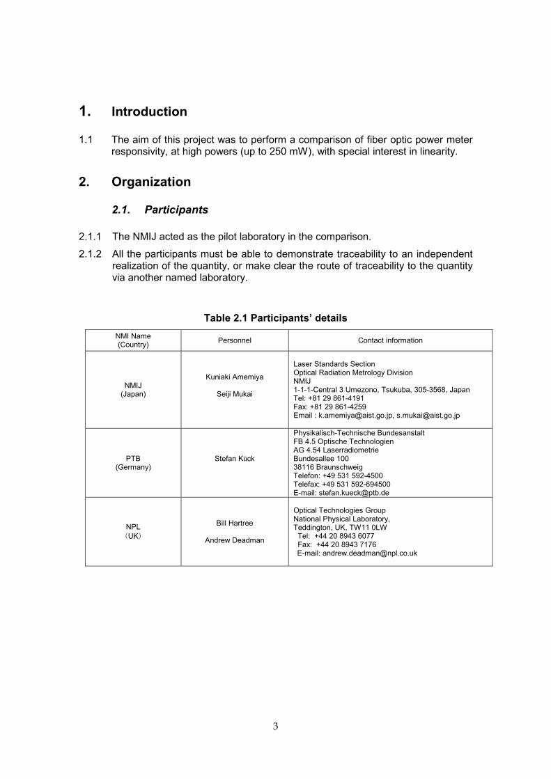
2.1.1 The NMIJ acted as the pilot laboratory in the comparison.

2.1.2 All the participants must be able to demonstrate traceability to an independent realization of the quantity, or make clear the route of traceability to the quantity via another named laboratory.

Table 2.1 Participants’ details

NMI Name (Country)

Personnel Contact information

NMIJ (Japan)

Kuniaki Amemiya

Seiji Mukai

Laser Standards Section Optical Radiation Metrology Division NMIJ 1-1-1-Central 3 Umezono, Tsukuba, 305-3568, Japan Tel: +81 29 861-4191 Fax: +81 29 861-4259 Email : [email protected], [email protected]

PTB (Germany)

Stefan Kück

Physikalisch-Technische Bundesanstalt FB 4.5 Optische Technologien AG 4.54 Laserradiometrie Bundesallee 100 38116 Braunschweig Telefon: +49 531 592-4500 Telefax: +49 531 592-694500 E-mail: [email protected]

NPL

（UK）

Bill Hartree

Andrew Deadman

Optical Technologies Group National Physical Laboratory, Teddington, UK, TW11 0LW Tel: +44 20 8943 6077 Fax: +44 20 8943 7176 E-mail: [email protected]

4

2.2. Form of comparison

2.3.1 The comparison was principally carried out through a fiber optic power meter.

2.3.2 A description of the power meter for use in this comparison is given in section 3 of this document. The fiber optic power meter consisted of an optical head, which was a photodiode/integrating sphere combination, a picoammeter as a display unit and an electrical cable connecting the two.

2.3.3 The fiber optic power meter was supplied by the NMIJ.

2.3.4 The comparison took the form of a star type comparison. The NMIJ calibrated the power meter and then sent it to one participant. The participant calibrated and returned the meter to NMIJ. The NMIJ recalibrated the meter to check for any drift during the comparison. The process was repeated until all the other participants finished the calibration.

2.3.5 Each participant was to send the fiber optic power responsivity and linearity at 1550 nm with the fiber optic power meter to the NMIJ as soon as possible after finishing the calibration.

2.3.6 The timetable given below shows an overview on how the comparison was planned.

2.3.7 Each laboratory had two months for calibration and transportation.

2.3. Timetable (on the technical protocol)

Table 2.2 Timetable (on the technical protocol)

Activity Start Date End Date

Circulation of technical protocol and invitation of participants to members

January 2008 30 April 2008

Confirmation of participation by member labs and revision of protocol

30 April 2008 June 2008

Submission of technical protocol to TCPR chair for approval

July 2008

Final revision and announcement of kick-off

Calibration of NMI 1 (NMIJ, JAPAN) October 2008

Calibration of NMI 2 (PTB, Germany) January 2009

Calibration of NMI 3 (NPL, UK) April 2009

Draft A report August 2009

Draft B report April 2010

5

Table 2.3 Total schedule and data of the comparison.

Country Receipt

Confirmation Damage

Completion Confirmation

Damage /Remarks

Description of facility

Results

JP 2008.12.1 No 2009.1.8 No 2009.1.8 2009.1.8

DE 2009.1.27 Yes* 2009.5.1 Repaired** 2010.4.15 2010.4.15

JP 2009.5.22 No 2009.6.9 No 2009.6.9 2009.6.9

UK 2009.6.22 No 2009.11.16 No 2010.6.1 2010.6.1

JP 2009.12.9 No 2010.1.31 No 2010.1.31 2010.1.31

*The port plug was dropped into the integrating sphere **Repaired according to the instruction by the pilot laboratory

2.4. Remarks

PTB reported a problem with the power meter. The integrating sphere port plug had fallen into the integrating sphere. This was probably because the material of the port plug shrank due to the low temperature encountered during air transportation. The plug was repaired by PTB after instruction from the pilot laboratory. After PTB’s measured and returned the power meter to the pilot laboratory, the responsivity as well as the nonlinearity was tested. No significant changes were found, as described in Section 3.2. Therefore, the pilot laboratory concluded that the measurements performed by PTB were valid for this comparison.

3. Description of the standards

3.1. Artefact

3.1.1 The measurement artefact was a fiber optic power meter, which consisted of an optical head with an FC type fiber optic connector end, a display unit, and an electrical cable connecting them. The display unit has an input port to connect to the output port of the optical head and an LED display panel indicating the output current of the optical head in electrical current unit (nA and µA).

3.1.2 The fiber optic power meter is sensitive to dust and pollution. When not used it must be stored with the cover closed.

3.1.3 The fiber optic power meter is shown in Figure 3.1. The supply voltage is 100 V. The voltage and the plug may not be compatible with participant laboratories. Appropriate converting adaptor with the ground terminal may solve this problem.

3.1.4 A user manual of the fiber optic power meter is included so that the participants can refer to it.

6

Figure 3.1 Schematic of the fiber optic power meter

Mains cable

Plug

-----nA

Display Unit FC receptacle

Electrical cable

(Each participant’s own fiber optic patch cord)

Optical head

7

3.2. Performance of the Artefact

According to the technical protocol, section 5.4 (page 8), the draft A here describes

the performance of the transfer detectors. In order to evaluate the performance of the transfer detector, the responsivity and the nonlinearity of the detector was measured several times by the NMIJ (pilot laboratory) during this comparison. In the following, the detailed results for the detector and each measurand are listed in Table 3.1 - Table 3.2 and are shown in Figure 3.2 – Figure 3.3. The detector exhibits a slight change in the responsivity and the nonlinearity over time,

probably caused by the transport and/or the reproducibility during the measurements. Therefore it is suggested to take into account these changes in the responsivity and the nonlinearity for the evaluation of the results of the participants. This should be performed in the following way, i.e. using a linear interpolation based on the measurements carried out at the pilot lab (NMIJ):

( ) ( )avenn

sss ∆−⋅=∆+∆−⋅= − 12/)(1 NMI1NMI

*

NMI

where s

*NMI (sNMI) is the corrected (submitted) responsivity or nonlinearity for each

participating laboratory, ∆n-1 and ∆n are the deviation with respect to the mean spectral responsivities or nonlinearities measured at NMIJ before and after the individual measurement of the each participant, respectively. In Table 3.3 and Table 3.4 the

values for ∆ave are given for each NMI for the transfer detectors.

The maximum deviation for the corrections ∆ave are -0.037 % at 100 mW, 125 mW and 250 mW in fiber optic power

responsivity, -0.0090 % at 250 mW in nonlinearity.

8

Table 3.1 Performance of the transfer detector. ssssRRRR(NMIJ)(NMIJ)(NMIJ)(NMIJ)nnnn: normalized

responsivity (with respect to the mean value of the measurements performed at

NMIJ), UUUU((((ssssRRRR(NMIJ)(NMIJ)(NMIJ)(NMIJ)nnnn)))): expanded uncertainty, k: coverage factor, ∆R: deviation with

respect to the mean value (Fiber optic power responsivity)

1 mW sR(NMIJ)n U(sR(NMIJ)n) k ∆R,n

Dec-08 0.9996 0.08% 2.0 -0.04%

May-09 0.9998 0.14% 2.0 -0.02%

Jan-10 1.0006 0.18% 2.0 0.06%

mean 1.0000 0.13% 2.0 0.00%


Dec-08 0.9996 0.09% 2.0 -0.04%

May-09 0.9998 0.14% 2.0 -0.02%

Jan-10 1.0006 0.19% 2.0 0.06%

mean 1.0000 0.14% 2.0 0.00%


Dec-08 0.9995 0.11% 2.0 -0.05%

May-09 0.9998 0.15% 2.0 -0.02%

Jan-10 1.0007 0.19% 2.0 0.07%

mean 1.0000 0.15% 2.0 0.00%


Dec-08 0.9995 0.11% 2.0 -0.05%

May-09 0.9998 0.16% 2.0 -0.02%

Jan-10 1.0007 0.20% 2.0 0.07%

mean 1.0000 0.16% 2.0 0.00%


Dec-08 0.9995 0.11% 2.0 -0.05%

May-09 0.9998 0.15% 2.0 -0.02%

Jan-10 1.0007 0.20% 2.0 0.07%

mean 1.0000 0.15% 2.0 0.00%

9

Figure 3.2 The following figures show the performance of the transfer detector

for the different measurands (power levels) at NMIJ over the time of the

comparison, normalized to the mean value of the measurements performed at

NMIJ (Fiber optic power responsivity).

1 mW

0.997

0.998

0.999

1

1.001

1.002

1.003

Dec-08 Mar-09 Jun-09 Sep-09 Dec-09

Date

Rela

tive

spe

ctr

al r

esp

onsi

vity

10 mW

0.997

0.998

0.999

1

1.001

1.002

1.003


Date

Rela

tive

spe

ctr

al r

esp

onsi

vity

10

100 mW

0.997

0.998

0.999

1

1.001

1.002

1.003


Date

Rela

tive

spe

ctr

al r

esp

onsi

vity

125 mW

0.997

0.998

0.999

1

1.001

1.002

1.003


Date

Rela

tive

spe

ctr

al r

esp

onsi

vity

11

250 mW

0.997

0.998

0.999

1

1.001

1.002

1.003


Date

Rela

tive

spe

ctr

al r

esp

onsi

vity

0.997

0.998

0.999

1

1.001

1.002

1.003


Date

Rela

tive

spe

ctr

al r

esp

onsi

vity

1 mW

10 mW

100 mW

125 mW

250 mW

12

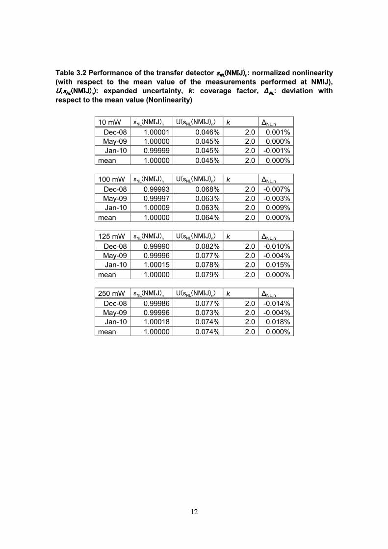
Table 3.2 Performance of the transfer detector ssssNLNLNLNL(NMI(NMI(NMI(NMIJ)J)J)J)nnnn: normalized nonlinearity

(with respect to the mean value of the measurements performed at NMIJ),

UUUU((((ssssNLNLNLNL(NMI(NMI(NMI(NMIJ)J)J)J)nnnn)))): expanded uncertainty, k: coverage factor, ∆NLNLNLNL: deviation with

respect to the mean value (Nonlinearity)

10 mW sNL(NMIJ)n U(sNL(NMIJ)n) k ∆NL,n

Dec-08 1.00001 0.046% 2.0 0.001%

May-09 1.00000 0.045% 2.0 0.000%

Jan-10 0.99999 0.045% 2.0 -0.001%

mean 1.00000 0.045% 2.0 0.000%


Dec-08 0.99993 0.068% 2.0 -0.007%

May-09 0.99997 0.063% 2.0 -0.003%

Jan-10 1.00009 0.063% 2.0 0.009%

mean 1.00000 0.064% 2.0 0.000%


Dec-08 0.99990 0.082% 2.0 -0.010%

May-09 0.99996 0.077% 2.0 -0.004%

Jan-10 1.00015 0.078% 2.0 0.015%

mean 1.00000 0.079% 2.0 0.000%


Dec-08 0.99986 0.077% 2.0 -0.014%

May-09 0.99996 0.073% 2.0 -0.004%

Jan-10 1.00018 0.074% 2.0 0.018%

mean 1.00000 0.074% 2.0 0.000%

13

Figure 3.3 The following figures show the performance of the transfer detector

for the different measurands (power levels) at NMIJ over the time of the

comparison, normalized to the mean value of the measurements performed at

NMIJ (Nonlinearity).

10 mW

0.9990

0.9992

0.9994

0.9996

0.9998

1.0000

1.0002

1.0004

1.0006

1.0008

1.0010


Date

Rela

tive

lin

ear

ity

facto

r

100 mW

0.9990

0.9992

0.9994

0.9996

0.9998

1.0000

1.0002

1.0004

1.0006

1.0008

1.0010


Date

Rela

tive

lin

ear

ity

facto

r

14

125 mW

0.9990

0.9992

0.9994

0.9996

0.9998

1.0000

1.0002

1.0004

1.0006

1.0008

1.0010


Date

Rela

tive

lin

ear

ity

facto

r

250 mW

0.9990

0.9992

0.9994

0.9996

0.9998

1.0000

1.0002

1.0004

1.0006

1.0008

1.0010


Date

Rela

tive

lin

ear

ity

facto

r

15

Table 3.3 The mean deviation for the correction ∆R,ave for the transfer detector,

details see text. (Fiber optic power responsivity)

1 mW sR(NMIJ)n-1 sR(NMIJ)n ∆R,ave

PTB 0.9996 0.9998 -0.028%

NPL 0.9998 1.0006 0.020%

Max -0.028%


PTB 0.9996 0.9998 -0.028%

NPL 0.9998 1.0006 0.019%

Max -0.028%


PTB 0.9995 0.9998 -0.033%

NPL 0.9998 1.0007 0.023%

Max -0.033%


PTB 0.9995 0.9998 -0.036%

NPL 0.9998 1.0007 0.025%

Max -0.036%


PTB 0.9995 0.9998 -0.037%

NPL 0.9998 1.0007 0.027%

Max -0.037%

16

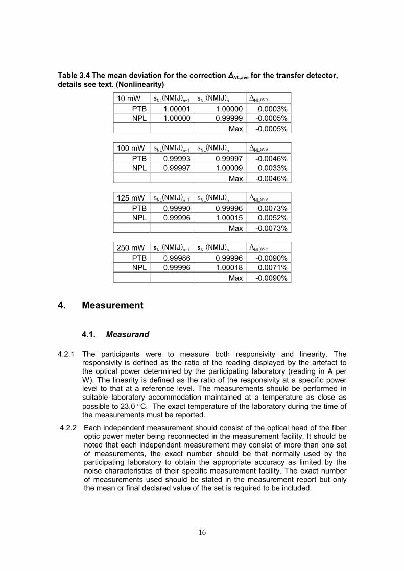
Table 3.4 The mean deviation for the correction ∆NL,ave for the transfer detector,

details see text. (Nonlinearity)

10 mW sNL(NMIJ)n-1 sNL(NMIJ)n ∆NL,ave

PTB 1.00001 1.00000 0.0003%

NPL 1.00000 0.99999 -0.0005%

Max -0.0005%


PTB 0.99993 0.99997 -0.0046%

NPL 0.99997 1.00009 0.0033%

Max -0.0046%


PTB 0.99990 0.99996 -0.0073%

NPL 0.99996 1.00015 0.0052%

Max -0.0073%


PTB 0.99986 0.99996 -0.0090%

NPL 0.99996 1.00018 0.0071%

Max -0.0090%

4. Measurement

4.1. Measurand

4.2.1 The participants were to measure both responsivity and linearity. The

responsivity is defined as the ratio of the reading displayed by the artefact to the optical power determined by the participating laboratory (reading in A per W). The linearity is defined as the ratio of the responsivity at a specific power level to that at a reference level. The measurements should be performed in suitable laboratory accommodation maintained at a temperature as close as

possible to 23.0 °C. The exact temperature of the laboratory during the time of the measurements must be reported.

4.2.2 Each independent measurement should consist of the optical head of the fiber optic power meter being reconnected in the measurement facility. It should be noted that each independent measurement may consist of more than one set of measurements, the exact number should be that normally used by the participating laboratory to obtain the appropriate accuracy as limited by the noise characteristics of their specific measurement facility. The exact number of measurements used should be stated in the measurement report but only the mean or final declared value of the set is required to be included.

17

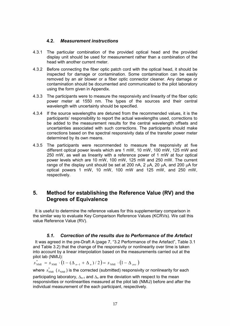
4.2. Measurement instructions

4.3.1 The particular combination of the provided optical head and the provided

display unit should be used for measurement rather than a combination of the head with another current meter.

4.3.2 Before connecting the fiber optic patch cord with the optical head, it should be inspected for damage or contamination. Some contamination can be easily removed by an air blower or a fiber optic connector cleaner. Any damage or contamination should be documented and communicated to the pilot laboratory using the form given in Appendix.

4.3.3 The participants were to measure the responsivity and linearity of the fiber optic power meter at 1550 nm. The types of the sources and their central wavelength with uncertainty should be specified.

4.3.4 If the source wavelengths are detuned from the recommended values, it is the participants’ responsibility to report the actual wavelengths used, corrections to be added to the measurement results for the central wavelength offsets and uncertainties associated with such corrections. The participants should make corrections based on the spectral responsivity data of the transfer power meter determined by its own means.

4.3.5 The participants were recommended to measure the responsivity at five different optical power levels which are 1 mW, 10 mW, 100 mW, 125 mW and 250 mW, as well as linearity with a reference power of 1 mW at four optical power levels which are 10 mW, 100 mW, 125 mW and 250 mW. The current range of the display unit should be set at 200 nA, 2 µA, 20 µA, and 200 µA for

optical powers 1 mW, 10 mW, 100 mW and 125 mW, and 250 mW, respectively.

5. Method for establishing the Reference Value (RV) and the

Degrees of Equivalence It is useful to determine the reference values for this supplementary comparison in

the similar way to evaluate Key Comparison Reference Values (KCRVs). We call this value Reference Value (RV).

5.1. Correction of the results due to Performance of the Artefact

It was agreed in the pre-Draft A (page 7, “3.2 Performance of the Artefact”, Table 3.1 and Table 3.2) that the change of the responsivity or nonlinearity over time is taken into account by a linear interpolation based on the measurements carried out at the pilot lab (NMIJ):

( ) ( )avenn

sss ∆−⋅=∆+∆−⋅= − 12/)(1 NMI1NMI

*

NMI

where *

NMIs ( NMIs ) is the corrected (submitted) responsivity or nonlinearity for each

participating laboratory, ∆n-1 and ∆n are the deviation with respect to the mean responsivities or nonlinearities measured at the pilot lab (NMIJ) before and after the individual measurement of the each participant, respectively.

18

The maximum deviation for the corrections ∆ave are -0.037 % at 100 mW, 125 mW and 250 mW in fiber optic power

responsivity, -0.0090 % at 250 mW in nonlinearity.

5.2. Determination of the cut-off, the RV and the Degrees of Equivalence

According to the Guidelines for CCPR Comparison Report Preparation, the default method for calculating RV is the weighted mean of the responsivity/nonlinearity values of all NMIs represent with cut-off. The cut-off value for the uncertainty, as a default, is determined as the average of the uncertainty values of those participants that reported uncertainties smaller than or equal to the median of all participants. In this comparison the cut-off uncertainty ucut-off is then the average of the uncertainties of two institutes stating the lowest uncertainties:

{ } 3...1;)(median)(for )}({average relrelreloffcut =≤=− ksususuukii

where urel(si) is the relative uncertainty reported by the participant i and the median is calculated from the three participants. In Table 5.1 the relative uncertainties of all participants for each measurand are listed together with the median value, the cut-off value and adjusted uncertainties determined as follows.

≤

≥=

−−

−

offcutreloffcut

offcutrelrel

adj)(for

)(for )()(

usuu

usususu

i

ii

i

The weight wi for the participant i is then calculated as

∑=

−

−

=3

1

2

adj

2

adj

)(

)(

i

i

i

i

su

suw .

The RV for the participants is calculated as

∑=

=3

1

*

RV

i

iisws

with the relative standard uncertainty

∑=

−

=3

1

2

adj

RVrel

)(

1)(

i

isu

su

The unilateral DoE of NMI i is given by

RV

RV

s

ssD

i

i

−=

with its expanded uncertainty

2;)()( 2

rel

2

RVrel =+= ksusukUii

The bilateral DoE between NMI i to NMI m is given by

RV

,s

ssDDD

mi

mimi

−=−=

with

19

2;)()()( 2

rel

2

rel

2

RVrel, =++= ksususukUmimi

For nonlinearity, the results were reported only by two institutions. Therefore the RV cannot be calculated and the bilateral DoE between the two institutions is given by

},{averge,

mi

mi

mi

ss

ssD

−=

with

2;)()( 2

rel

2

rel, =+= ksusukUmimi

20

Table 5.1 Relative uncertainty urel(si) of the fiber optic power responsity or nonlinearity for the artefact and each participant, the adjusted uncertainty

uadj(si), the weight wi, the median and the cut-off value of the uncertainty for each measurand.

Fiber Optic Power Responsivity

Nonlinearity

10 mW 100 mW 125 mW 250 mW

NMI urel(si) (%)

uadj(si) (%)

wi urel(si) (%)

uadj(si) (%)

wi urel(si) (%)

uadj(si) (%)

wi urel(si) (%)

uadj(si) (%)

wi

1

2 0.023 - - 0.031 - - 0.038 - - 0.036 - -

3 0.45 - - 0.60 - - 0.81 - - 0.89 - -

Median - - - -

Cut-off - - - - - - - -

urel(sRV) (%)

- urel(sRV) (%)

- urel(sRV) (%)

- urel(sRV) (%)

-

1 mW 10 mW 100 mW 125 mW 250 mW

NMI urel(si) (%)

uadj(si) (%)

wi urel(si) (%)

uadj(si) (%)

wi urel(si) (%)

uadj(si) (%)

wi urel(si) (%)

uadj(si) (%)

wi urel(si) (%)

uadj(si) (%)

wi

1 0.43 0.43 0.22 0.41 0.41 0.24 0.48 0.48 0.24 1.22 1.22 0.10 1.24 1.24 0.11

2 0.12 0.27 0.56 0.12 0.26 0.57 0.12 0.30 0.61 0.12 0.47 0.68 0.12 0.51 0.67

3 0.42 0.42 0.23 0.45 0.45 0.19 0.60 0.60 0.15 0.81 0.81 0.22 0.89 0.89 0.22

Median 0.42 0.41 0.48 0.81 0.89

Cut-off 0.27 1.00 0.26 1.00 0.30 1.00 0.47 1.00 0.51 1.00

urel(sRV) (%)

0.20 urel(sRV) (%)

0.20 urel(sRV) (%)

0.23 urel(sRV) (%)

0.38 urel(sRV) (%)

0.41

21

6. Identification of outliers According to “Guidelines for CCPR Comparison Report Preparation”, the pilot lab should discuss with all the participants about removal of outlier(s), where the RV value would be significantly skewed. The pilot lab circulated the relative results of each participant for each measurands (the

identification numbers there were random), and discussed about any proposal of outlier(s). There were no proposal of outlier(s), therefore all results were used to determine the reference values.

22

7. Results

7.1. Summary of participants’ results

In the Table 7.1 the reported results of all participants including the responsivities or nonlinearities, their uncertainties, their relative uncertainties and coverage factors are summarised. For the detail of each participant’s report, see Appendix D.

Table 7.1 Summary of participants’ results

Fiber optic power responsivity

Results of NMIJ (Japan)


Power s u(s) u(s) k

(mW) (A/W) (A/W)

1 9.879E-05 1.2E-07 0.12% 2.0

10 9.880E-05 1.2E-07 0.12% 2.0

100 9.863E-05 1.2E-07 0.12% 2.0

125 9.863E-05 1.2E-07 0.12% 2.0

250 9.863E-05 1.2E-07 0.12% 2.0

Results of PTB (Germany)


Power s u(s) u(s) k

(mW) (A/W) (A/W)

1 1.0009E-04 4.2E-07 0.42% 2.0

10 9.986E-05 4.5E-07 0.45% 2.0

100 9.958E-05 6.0E-07 0.60% 2.0

125 9.930E-05 8.0E-07 0.81% 2.0

250 9.920E-05 8.8E-07 0.89% 2.0

Results of NPL (United Kingdom)


Power s u(s) u(s) k

(mW) (A/W) (A/W)

1 9.829E-05 4.2E-07 0.43% 2.0

10 9.839E-05 4.0E-07 0.41% 2.0

100 9.832E-05 4.7E-07 0.48% 2.13

125 9.840E-05 1.20E-06 1.22% 2.0

250 9.840E-05 1.22E-06 1.24% 2.0

23

Nonlinearity

Results of NMIJ (Japan)

Nonlinearity

Power s u(s) u(s) k

(mW)

10 1.00008 0.00023 0.023% 2.0

100 0.99843 0.00031 0.031% 2.0

125 0.99841 0.00038 0.038% 2.0

250 0.99835 0.00036 0.036% 2.0

Results of PTB (Germany)

Nonlinearity

Power s u(s) u(s) k

(mW)

10 0.9977 0.0045 0.45% 2.0

100 0.9950 0.0060 0.60% 2.0

125 0.9921 0.0080 0.81% 2.0

250 0.9911 0.0088 0.89% 2.0

24

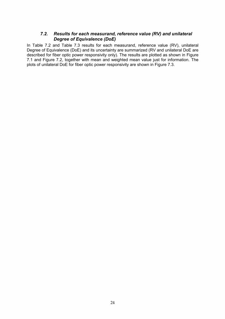
7.2. Results for each measurand, reference value (RV) and unilateral Degree of Equivalence (DoE)

In Table 7.2 and Table 7.3 results for each measurand, reference value (RV), unilateral Degree of Equivalence (DoE) and its uncertainty are summarized (RV and unilateral DoE are described for fiber optic power responsivity only). The results are plotted as shown in Figure 7.1 and Figure 7.2, together with mean and weighted mean value just for information. The plots of unilateral DoE for fiber optic power responsivity are shown in Figure 7.3.

25

Table 7.2 Results for each measurand, reference value (RV) and unilateral Degree of

Equivalence (DoE) together with its uncertainty (Fiber optic power responsivity)

1 mW

Participant si* urel(si) Di ui(Di) Ui(Di)

JP 9.879E-05 0.12% -0.19% 0.23% 0.46%

DE 1.0012E-04 0.42% 1.15% 0.47% 0.93%

GB 9.827E-05 0.43% -0.72% 0.47% 0.95%

RV 9.898E-05 0.20% 0.00% 0.20% 0.40%

10 mW


JP 9.880E-05 0.12% -0.11% 0.23% 0.47%

DE 9.989E-05 0.45% 0.99% 0.50% 0.99%

GB 9.837E-05 0.41% -0.54% 0.46% 0.91%

RV 9.891E-05 0.20% 0.00% 0.20% 0.40%

100 mW


JP 9.863E-05 0.12% -0.07% 0.26% 0.53%

DE 9.961E-05 0.60% 0.92% 0.65% 1.29%

GB 9.830E-05 0.48% -0.41% 0.53% 1.07%

RV 9.870E-05 0.23% 0.00% 0.23% 0.47%

125 mW


JP 9.863E-05 0.12% -0.13% 0.40% 0.81%

DE 9.934E-05 0.81% 0.58% 0.90% 1.79%

GB 9.838E-05 1.22% -0.39% 1.28% 2.56%

RV 9.876E-05 0.38% 0.00% 0.38% 0.77%

250 mW


JP 9.863E-05 0.12% -0.10% 0.43% 0.87%

DE 9.924E-05 0.89% 0.51% 0.98% 1.96%

GB 9.837E-05 1.24% -0.36% 1.31% 2.62%

RV 9.873E-05 0.41% 0.00% 0.41% 0.83%

26

Table 7.3 Results for each measurand together with its uncertainty (Nonlinearity)

10 mW


JP 1.00008 0.023% - - -

DE 0.9977 0.45% - - -

GB - - - - -

RV - - - - -

100 mW


JP 0.99843 0.031% - - -

DE 0.9950 0.60% - - -

GB - - - - -

RV - - - - -

125 mW


JP 0.99841 0.038% - - -

DE 0.9922 0.81% - - -

GB - - - - -

RV - - - - -

250 mW


JP 0.99835 0.036% - - -

DE 0.9912 0.89% - - -

GB - - - - -

RV - - - - -

27

Figure 7.1 Results for each measurand, mean, weighted mean and reference value

(RV)


1 mW

9.50E-05

9.60E-05

9.70E-05

9.80E-05

9.90E-05

1.00E-04

1.01E-04

1.02E-04

Resp

onsi

vity

(A

/W

)

1 mW

1 mW 9.879E-05 1.0012E-04 9.827E-05 9.906E-05 9.885E-05 9.898E-05

JP DE GB meanweighted

meanRV

10 mW

9.50E-05

9.60E-05

9.70E-05

9.80E-05

9.90E-05

1.00E-04

1.01E-04

1.02E-04

Resp

onsi

vity

(A

/W

)

10 mW

10 mW 9.880E-05 9.989E-05 9.837E-05 9.902E-05 9.883E-05 9.891E-05


meanRV

28

100 mW

9.50E-05

9.60E-05

9.70E-05

9.80E-05

9.90E-05

1.00E-04

1.01E-04

1.02E-04

Resp

onsi

vity

(A

/W

)

100 mW

100 mW 9.863E-05 9.961E-05 9.830E-05 9.885E-05 9.865E-05 9.870E-05


meanRV

125 mW

9.50E-05

9.60E-05

9.70E-05

9.80E-05

9.90E-05

1.00E-04

1.01E-04

1.02E-04

Resp

onsi

vity

(A

/W

)

125 mW

125 mW 9.863E-05 9.934E-05 9.838E-05 9.878E-05 9.864E-05 9.876E-05


meanRV

250 mW

9.50E-05

9.60E-05

9.70E-05

9.80E-05

9.90E-05

1.00E-04

1.01E-04

1.02E-04

Resp

onsi

vity

(A

/W

)

250 mW

250 mW 9.863E-05 9.924E-05 9.837E-05 9.875E-05 9.864E-05 9.873E-05


meanRV

29

Figure 7.2 Results for each measurand, mean and weighted mean

Nonlinearity

10 mW

9.700E-01

9.750E-01

9.800E-01

9.850E-01

9.900E-01

9.950E-01

1.000E+00

1.005E+00

1.010E+00

1.015E+00

Nonlin

ear

ity

10 mW

10 mW 1.00008 0.9977 0.99889 1.00007


mean

100 mW

9.700E-01

9.750E-01

9.800E-01

9.850E-01

9.900E-01

9.950E-01

1.000E+00

1.005E+00

1.010E+00

1.015E+00

Nonlin

ear

ity

100 mW

100 mW 0.99843 0.9950 0.99674 0.99842


mean

30

125 mW

9.700E-01

9.750E-01

9.800E-01

9.850E-01

9.900E-01

9.950E-01

1.000E+00

1.005E+00

1.010E+00

1.015E+00

Nonlin

ear

ity

125 mW

125 mW 0.99841 0.9922 0.99529 0.99839


mean

250 mW

9.700E-01

9.750E-01

9.800E-01

9.850E-01

9.900E-01

9.950E-01

1.000E+00

1.005E+00

1.010E+00

1.015E+00

Nonlin

ear

ity

250 mW

250 mW 0.99835 0.9912 0.99477 0.99834


mean

31

Figure 7.3 Unilateral DoE: Fiber optic power responsivity

1 mW

-3.0%

-2.0%

-1.0%

0.0%

1.0%

2.0%

3.0%

JP DE GB

DoE

1 mW

10 mW

-3.00%

-2.00%

-1.00%

0.00%

1.00%

2.00%

3.00%

JP DE GB

DoE 10 mW

100 mW

-3.00%

-2.00%

-1.00%

0.00%

1.00%

2.00%

3.00%

JP DE GB

DoE

100 mW

32

125 mW

-3.00%

-2.00%

-1.00%

0.00%

1.00%

2.00%

3.00%

JP DE GB

DoE

125 mW

250 mW

-3.00%

-2.00%

-1.00%

0.00%

1.00%

2.00%

3.00%

JP DE GB

DoE

250 mW

33

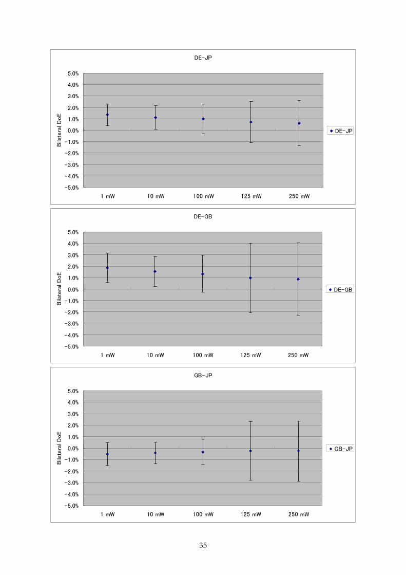
7.3. Bilateral Degree of Equivalence

Bilateral Degree of Equivalences of each measurand are listed In Table 7.4 and depicted as shown in Figure 7.4 and Figure 7.5.

Table 7.4 Bilateral Degree of Equivalence

Bilateral DoE, Di,j JP DE GB

JP Di,j Ui,j Di,j Ui,j Di,j Ui,j

Responsivity, 1 mW -1.34% 0.96% 0.52% 0.98%

Responsivity, 10 mW -1.10% 1.02% 0.43% 0.94%

Responsivity, 100 mW -1.00% 1.32% 0.34% 1.10%

Responsivity, 125 mW -0.71% 1.81% 0.26% 2.57%

Responsivity, 250 mW -0.61% 1.98% 0.26% 2.63%

Nonlinearity, 10 mW 0.24% 0.91%





DE Di,j Ui,j Di,j Ui,j Di,j Ui,j

Responsivity, 1 mW 1.34% 0.96% 1.87% 1.27%

Responsivity, 10 mW 1.10% 1.02% 1.53% 1.29%

Responsivity, 100 mW 1.00% 1.32% 1.33% 1.61%

Responsivity, 125 mW 0.71% 1.81% 0.97% 3.03%

Responsivity, 250 mW 0.61% 1.98% 0.87% 3.16%

Nonlinearity, 10 mW -0.24% 0.91%





GB Di,j Ui,j Di,j Ui,j Di,j Ui,j

Responsivity, 1 mW -0.53% 0.98% -1.87% 1.27%

Responsivity, 10 mW -0.43% 0.94% -1.53% 1.29%

Responsivity, 100 mW -0.34% 1.10% -1.33% 1.61%

Responsivity, 125 mW -0.26% 2.57% -0.97% 3.03%

Responsivity, 250 mW -0.26% 2.63% -0.87% 3.16%

Nonlinearity, 10 mW

Nonlinearity, 100 mW



34

Figure 7.4 Bilateral Degree of Equivalence (Fiber optic power responsivity)

JP-DE

-5.0%

-4.0%

-3.0%

-2.0%

-1.0%

0.0%

1.0%

2.0%

3.0%

4.0%

5.0%

1 mW 10 mW 100 mW 125 mW 250 mW

Bila

tera

l D

oE

JP-DE

JP-GB

-5.0%

-4.0%

-3.0%

-2.0%

-1.0%

0.0%

1.0%

2.0%

3.0%

4.0%

5.0%

1 mW 10 mW 100 mW 125 mW 250 mW

Bila

tera

l D

oE

JP-GB

35

DE-JP

-5.0%

-4.0%

-3.0%

-2.0%

-1.0%

0.0%

1.0%

2.0%

3.0%

4.0%

5.0%

1 mW 10 mW 100 mW 125 mW 250 mW

Bila

tera

l D

oE

DE-JP

DE-GB

-5.0%

-4.0%

-3.0%

-2.0%

-1.0%

0.0%

1.0%

2.0%

3.0%

4.0%

5.0%

1 mW 10 mW 100 mW 125 mW 250 mW

Bila

tera

l D

oE

DE-GB

GB-JP

-5.0%

-4.0%

-3.0%

-2.0%

-1.0%

0.0%

1.0%

2.0%

3.0%

4.0%

5.0%

1 mW 10 mW 100 mW 125 mW 250 mW

Bila

tera

l D

oE

GB-JP

36

GB-DE

-5.0%

-4.0%

-3.0%

-2.0%

-1.0%

0.0%

1.0%

2.0%

3.0%

4.0%

5.0%

1 mW 10 mW 100 mW 125 mW 250 mW

Bila

tera

l D

oE

GB-DE

37

Figure 7.5 Bilateral Degree of Equivalence (Nonlinearity)

JP-DE

-3.00%

-2.00%

-1.00%

0.00%

1.00%

2.00%

3.00%

10 mW 100 mW 125 mW 250 mW

Bila

tera

l D

oE

JP-DE

DE-JP

-3.00%

-2.00%

-1.00%

0.00%

1.00%

2.00%

3.00%

10 mW 100 mW 125 mW 250 mW

Bila

tera

l D

oE

DE-JP

38

8. Conclusions The APMP.PR-S4 comparison of fiber optic power responsivity and nonlinearity at 1550 nm, from 1 mW to 250 mW was carried out. In total three institute participated: NMIJ (Japan), PTB (Germany) and NPL (United Kingdom). The measurements started from December 2008, and ended on December 2009. For fiber optic power responsivity, all participants reported their results and all results are used for the intercomparison: no measurement was subject of rejection. For nonlinearity two participants reported their results, therefore only bilateral comparison was performed. The analysis method as mentioned in Section 5 was according to the Guidelines for CCPR Comparison Report Preparation, and has been accepted by all participants. Reference Value (RV) of fiber optic power responsivity was calculated using all participants’ results and no participants had to be excluded. For fiber optic power from 10 mW to 250 mW all participants had unilateral DoEs with values consistent their uncertainty at the k=2 level. At fiber optic power of 1 mW all participants achieved consistency at the k=3 level. For nonlinearity, the consistency of the measurements at both NMIJ and PTB resulted in uncertainty at the k=2 level.

39

9. Appendix A: List of Figures Figure 3.1 Schematic of the fiber optic power meter .............................................................. 6

Figure 3.2 The following figures show the performance of the transfer detector for the different measurands (power levels) at NMIJ over the time of the comparison, normalized to the mean value of the measurements performed at NMIJ (Fiber optic power responsivity). ............................................................................................................. 9

Figure 3.3 The following figures show the performance of the transfer detector for the different measurands (power levels) at NMIJ over the time of the comparison, normalized to the mean value of the measurements performed at NMIJ (Nonlinearity). ...................................................................................................................... 13

Figure 7.1 Results for each measurand, mean, weighted mean and reference value (RV)....................................................................................................................................... 27

Figure 7.2 Results for each measurand, mean and weighted mean ................................. 29

Figure 7.3 Unilateral DoE: Fiber optic power responsivity ................................................... 31

Figure 7.4 Bilateral Degree of Equivalence (Fiber optic power responsivity) ................... 34

Figure 7.5 Bilateral Degree of Equivalence (Nonlinearity) ................................................... 37

40

10. Appendix B: List of Tables Table 2.1 Participants’ details..................................................................................................... 3

Table 2.2 Timetable (on the technical protocol) ...................................................................... 4

Table 2.3 Total schedule and data of the comparison. .......................................................... 5

Table 3.1 Performance of the transfer detector. s(NMIJ)n: normalized responsivity (with

respect to the mean value of the measurements performed at NMIJ), U(s(NMIJ)n): expanded uncertainty, k: coverage factor, ∆: deviation with respect to the mean value (Fiber optic power responsivity) ............................................................................... 8

Table 3.2 Performance of the transfer detector s(NMIJ)n: normalized nonlinearity (with

respect to the mean value of the measurements performed at NMIJ), U(s(NMIJ)n): expanded uncertainty, k: coverage factor, ∆: deviation with respect to the mean value (Nonlinearity)............................................................................................................. 12

Table 3.3 The mean deviation for the correction ∆ave for the transfer detector, details see text. (Fiber optic power responsivity)............................................................................... 15

Table 3.4 The mean deviation for the correction ∆ave for the transfer detector, details see text. (Nonlinearity) .............................................................................................................. 16

Table 5.1 Relative uncertainty urel(si) of the fiber optic power responsity or nonlinearity for the artefact and each participant, the adjusted uncertainty uadj(si), the weight wi, the median and the cut-off value of the uncertainty for each measurand. ................ 20

Table 7.1 Summary of participants’ results ............................................................................ 22

Table 7.2 Results for each measurand, reference value (RV) and unilateral Degree of Equivalence (DoE) together with its uncertainty (Fiber optic power responsivity) ... 25

Table 7.3 Results for each measurand together with its uncertainty (Nonlinearity) ........ 26

Table 7.4 Bilateral Degree of Equivalence ............................................................................. 33

41

11. Appendix C: Timeline of the comparison

Technical Protocol agreed: 2008-08-06 Start of Measurements: 2008-12-01 End of Measurements: 2010-01-31 All reports received: 2010-06-01 Pre-Draft “A” published: 2010-07-06 First draft of Draft “A” 2011-01-10 Second draft of Draft “A” 2011-05-24 Draft “A” agreed: 2011-06-09 Draft “B” submitted: 2011-06-29 Draft “B” approved: 2011-07-28 Final report submitted: 2011-07-28

42

12. Appendix D: Measurement reports and uncertainty tables of

the participants 1. NMIJ, Japan, JP 2. PTB, Germany, DE 3. NPL, United Kingdom, GB

Report of the calibration performed by NReport of the calibration performed by NReport of the calibration performed by NReport of the calibration performed by NMIJMIJMIJMIJ of the fibre opti of the fibre opti of the fibre opti of the fibre optic power meter c power meter c power meter c power meter transfer standardtransfer standardtransfer standardtransfer standard of the APMP of the APMP of the APMP of the APMP----PR.S4PR.S4PR.S4PR.S4 intercomparison intercomparison intercomparison intercomparison

ScopeScopeScopeScope The participants were recommended to measure the responsivity at five

different optical power levels which are 1 mW, 10 mW, 100 mW, 125 mW, and 250 mW, as well as linearity with a reference power of 1 mW at four optical power levels which are 10 mW, 100 mW, 125 mW, and 250 mW. The current range of the display unit should be set at 200 nA, 2 µA, 20 µA, and 200 µA for optical powers 1 mW, 10 mW, 100 mW and 125 mW, and 250 mW, respectively. ArtefactArtefactArtefactArtefact The measurement artefact that is the fiber optic power meter will consist of a fiber

optic patch cord with FC/APC type connector, an optical head to accept the FC type fiber optic connector end, a display unit, and an electrical cable connecting them. The display unit provides with an input port to connect the output port of the optical head and an LED display panel indicating the output current of the optical head in electrical current unit.

Figure 1: Artefact for APMP.PRFigure 1: Artefact for APMP.PRFigure 1: Artefact for APMP.PRFigure 1: Artefact for APMP.PR----S4 comparison.S4 comparison.S4 comparison.S4 comparison.

NMIJ WORKING STANDARD FOR OPTICAL FIBER POWER: OPTICAL FIBER NMIJ WORKING STANDARD FOR OPTICAL FIBER POWER: OPTICAL FIBER NMIJ WORKING STANDARD FOR OPTICAL FIBER POWER: OPTICAL FIBER NMIJ WORKING STANDARD FOR OPTICAL FIBER POWER: OPTICAL FIBER POWER CALORIMETERPOWER CALORIMETERPOWER CALORIMETERPOWER CALORIMETER As schematically illustrated in Fig. 2, the NMIJ working standard for optical fiber

power, optical fiber power calorimeter, consists of the main body and a detachable adaptor for optical fiber power input. The structure of the main body is similar to the Japan’s national standard of open beam laser power [1]. We measure optical power with the calorimeter by electrothermal substitution technique under isothermal temperature control. The advantage of the electrothermal substitution is that we can translate input optical power into electrical power output, which is traceable to much more precise standards of electricity. Isothermal temperature control of the optical absorber with heater and Pertier element enables us to eliminate the fluctuation driven by convectional or radiation loss of heat on the optical absorber since the temperature of the optical absorber is kept same with the ambient temperature, therefore measurement uncertainty would be more reduced than the system without isothermal temperature control. This type of calorimeter is equipped with NiP ultra-black absorber [2]; its reflectance is less than 0.2 %. The calorimeter also has the compensative absorber [3] to eliminate the effect from ambient temperature and/or

-----nA


Electrical cable

Fiber optic patch cord Mains cable

Plug

Optical head

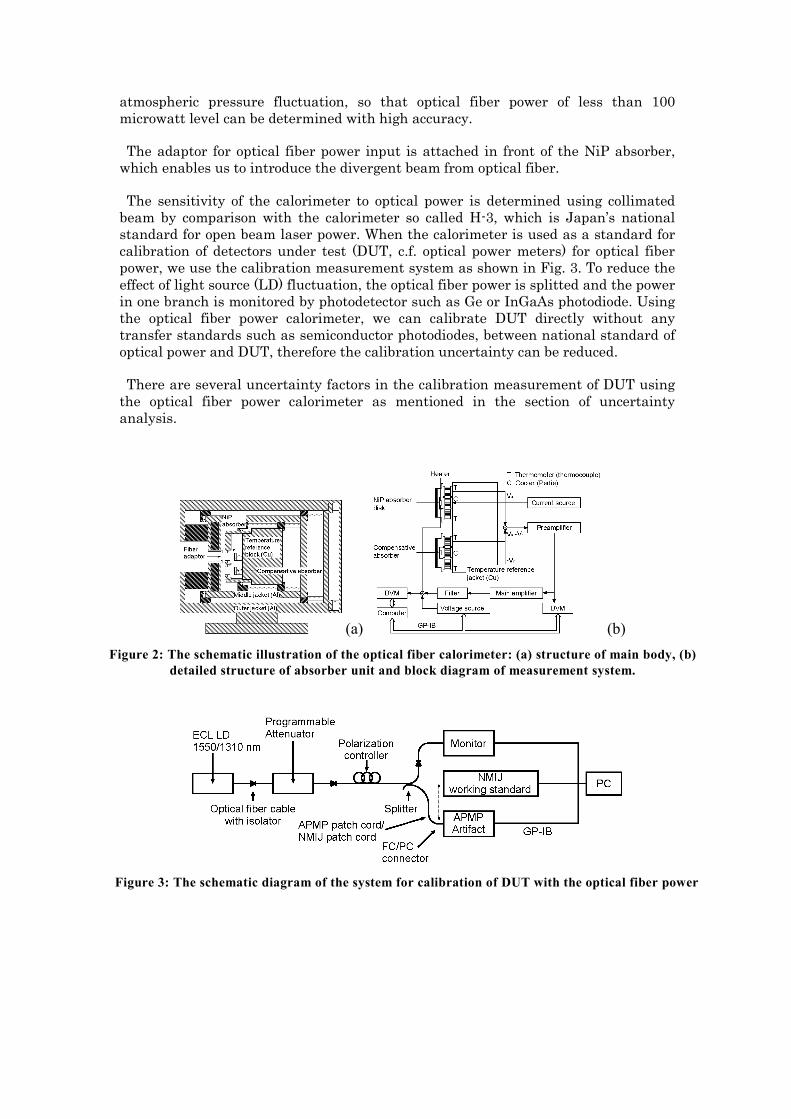
atmospheric pressure fluctuation, so that optical fiber power of less than 100 microwatt level can be determined with high accuracy.

The adaptor for optical fiber power input is attached in front of the NiP absorber, which enables us to introduce the divergent beam from optical fiber.

The sensitivity of the calorimeter to optical power is determined using collimated beam by comparison with the calorimeter so called H-3, which is Japan’s national standard for open beam laser power. When the calorimeter is used as a standard for calibration of detectors under test (DUT, c.f. optical power meters) for optical fiber power, we use the calibration measurement system as shown in Fig. 3. To reduce the effect of light source (LD) fluctuation, the optical fiber power is splitted and the power in one branch is monitored by photodetector such as Ge or InGaAs photodiode. Using the optical fiber power calorimeter, we can calibrate DUT directly without any transfer standards such as semiconductor photodiodes, between national standard of optical power and DUT, therefore the calibration uncertainty can be reduced.

There are several uncertainty factors in the calibration measurement of DUT using the optical fiber power calorimeter as mentioned in the section of uncertainty analysis.

(a) (b)

Figure 2: The schematic illustration of the optical fiber calorimeter: (a) structure of main body, (b)

detailed structure of absorber unit and block diagram of measurement system.

Figure 3: The schematic diagram of the system for calibration of DUT with the optical fiber power

NonlNonlNonlNonlinearity inearity inearity inearity calibration calibration calibration calibration systemsystemsystemsystem ( ( ( (Superposition methodSuperposition methodSuperposition methodSuperposition method))))

The nonlinearity of test optical power meter was calibrated by superposition method, as shown in Fig. 4. In the superposition method, optical powers through optical switch 1 and 2 are superimposed in the test power meter. Adjusting optical attenuator, each same optical power reading on the test meter via switch 1 or 2 can be obtained. Applying both of optical power through switch 1 and 2, the meter should indicate double of the reading with applying single optical power. Non-linearity of the test meter is determined from the shift of actual reading relative to double of single power reading. By changing optical attenuator setting to shift power level and then repeating same procedures in tern, non-linearity of the test meter can be calibrated in wide dynamic range. For exact 10 dB calibration, single power reading and actual reading for 4 times of single power application are superimposed (in other words, 1+4=5). We can 10 dB power ratio from “5+5”. --- For range discontinuity measurments, 1 mW was measured at 1 mW range and 10 mW range, 10 mW was measured at 10 mW range and 100 mW range and then 100 mW was measured at 100 mW range and 1 W range. Range discontinuity was measured by, for example, local linearity factor (LF) = reading at 10 mW range/ reading at 1 mW range when applying 1 mW.

FigFigFigFigureureureure 4444: : : : NonlNonlNonlNonlinearity calibration system for sinearity calibration system for sinearity calibration system for sinearity calibration system for standard power tandard power tandard power tandard power meter bymeter bymeter bymeter by superposition method.superposition method.superposition method.superposition method.

Optical power meter

PC

GP-IB

SW2

SW

Optical attenuators with optical

Light Source 1

Light Source 2

UncUncUncUncertainty analysesertainty analysesertainty analysesertainty analyses (1) fiber optic power Calibration measurement uncertainty using the NMIJ optical fiber power calorimeter was evaluated for 1 mW, 1550 nm. The uncertainties were evaluated in accordance with international document standards [4]. The results are summarized in Table 1. First, the calorimeter was calibrated with open beam of 1550 nm from laser diode at

1 mW using the laser power national standard, therefore there are sensitivity calibration uncertainties, including the uncertainty of the national standard and standard deviation of the measurement for the calibration; 0.073%. Beam incident position also causes another uncertainty because of the non-

uniformity of NiP absorber. Detachable adapter would be exchanged periodically (typically once a year) for sensitivity calibration with open beam using laser power national standard, therefore the position of beam center from optical fiber on NiP absorber may be fluctuated. The uniformity of sensitive area of the absorber was examined by measuring open beam power with scanning 0.5 mm x 0.5 mm area on the absorber. The result was translated into the uncertainty of 0.077 %. These uncertainties mentioned above are common to the uncertainty of open beam

laser power calorimeter. There are other uncertainty factors unique for the measurement of fiber optical power, because of the divergent nature of its beam. One is the divergent incidence on the NiP absorber. Sensitivity calibration of the

calorimeter is performed with collimated beam; therefore, divergent incidence from optical fiber to the absorber would cause uncertainty since the reflectance of NiP would vary with incident angle of optical power. Relation between reflectance of NiP and incident angle of optical power was measured using the setup shown in Figure 5 (boxed). Collimated beam was introduced into integrating sphere, equipped with NiP absorber at the center of the sphere. Rotating the direction of NiP absorber surface, we measure the optical power reflected by the NiP with InGaAs photodiode. The results were shown in Figure 3; Reflectance was normalized by the value at 0 degree (normal incidence). The reflectance goes up to 1.7 with 30 degree incidence. However, according to the measurement of beam pattern emitted from optical fiber end, as shown in Figure 6, optical power of more than 99.99% is within +/− 10 degree direction from normal incidence, therefore the difference of the reflectance is only about 10 % between beam center and edge. Since the reflectance itself is quite small (0.1 - 0.2 %), the uncertainty driven by the angular incident of optical power is less than 0.001%. Another factor is multi-reflection between NiP absorber and the inner wall of the

fiber adaptor, which also arises from the divergent incidence. If the NiP absorber shows completely diffusive reflection, the multi-reflection is negligible. However, actual NiP absorber reflects a part of incident optical power to the specular direction rather than diffusively. That causes another uncertainty for the fiber optical power measurements. The uncertainty calculated with the beam pattern as shown in Figure 6 was 0.012 %. The uncertainty due to DC voltage meter used to measure the heater power in

electrical substitution technique was 0.018 % according to the specification of manufacturer. The optical fiber power calorimeter is operated in isothermal temperature control

with proportional feedback; therefore there is deviation due to the control. The uncertainty from the control was found to be 0.008 % by the experiment. Combining all of the uncertainty mentioned above and standard deviation of

comparison measurements (0.045 %, n=5), the expanded uncertainty for the calibration measurement of the APMP artifact for 1 mW, 1550 nm using the optical fiber power calorimeter was 0.22 % (k=2).

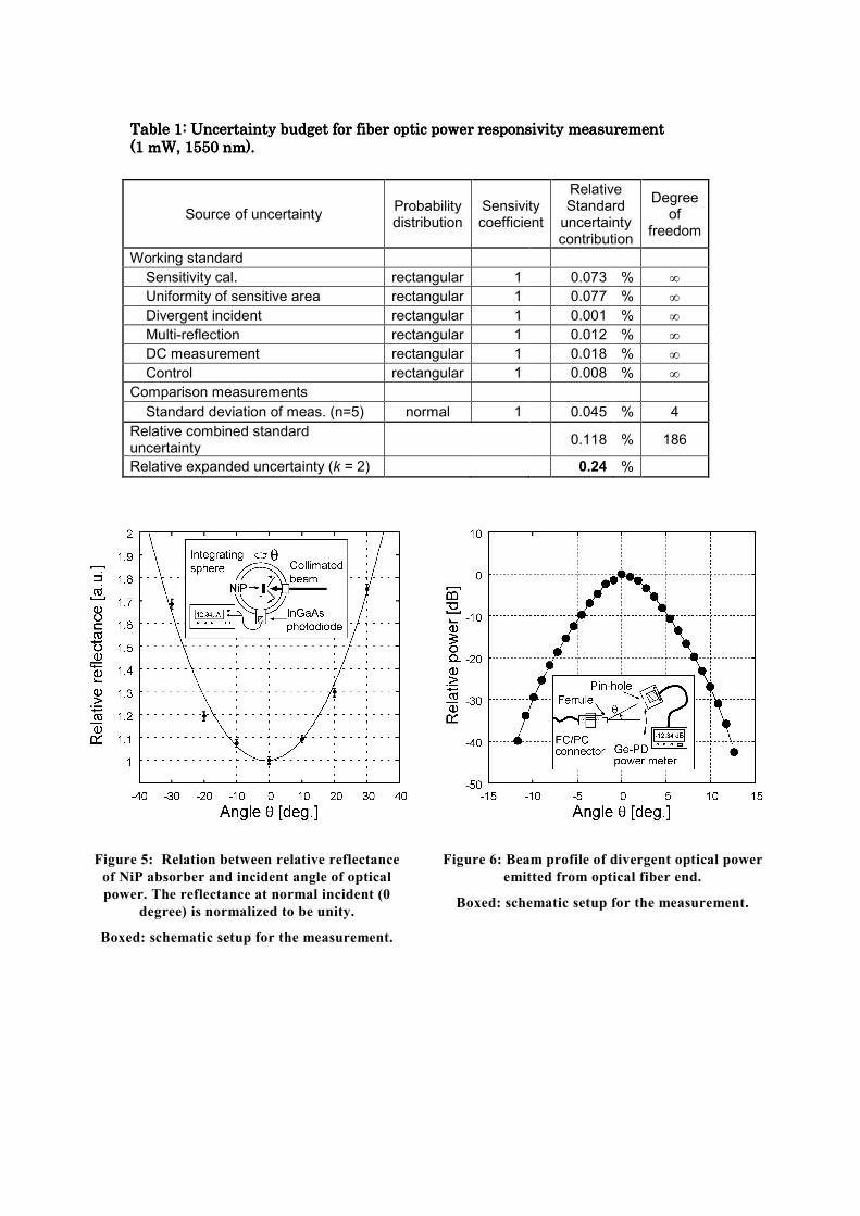
Table 1: Uncertainty budget for fiber optic power responsivity measTable 1: Uncertainty budget for fiber optic power responsivity measTable 1: Uncertainty budget for fiber optic power responsivity measTable 1: Uncertainty budget for fiber optic power responsivity measurementurementurementurement (1 mW, 1550 nm).(1 mW, 1550 nm).(1 mW, 1550 nm).(1 mW, 1550 nm).

Source of uncertainty Probability distribution

Sensivity coefficient

Relative Standard uncertainty contribution

Degree of

freedom

Working standard

Sensitivity cal. rectangular 1 0.073 % ∞

Uniformity of sensitive area rectangular 1 0.077 % ∞

Divergent incident rectangular 1 0.001 % ∞

Multi-reflection rectangular 1 0.012 % ∞

DC measurement rectangular 1 0.018 % ∞

Control rectangular 1 0.008 % ∞

Comparison measurements

Standard deviation of meas. (n=5) normal 1 0.045 % 4

Relative combined standard uncertainty

0.118 % 186

Relative expanded uncertainty (k = 2) 0.24 %

Figure 6: Beam profile of divergent optical power

emitted from optical fiber end.

Boxed: schematic setup for the measurement.

Figure 5: Relation between relative reflectance

of NiP absorber and incident angle of optical

power. The reflectance at normal incident (0

degree) is normalized to be unity.

Boxed: schematic setup for the measurement.

(2) Nonlinearity Nonlinearity of test power meter was calibrated by superposition method, as shown

in Fig. 1. The uncertainty due to the superposition method has several components of 1) source stability, 2) polarization dependence, 3) temperature fluctuation, 4) power level setting and 5) repeatability. Each uncertainty components were estimated as follows:

1) Source stability

In the system of high power calibration, the output power drifts dramatically especially due to temperature rise of optical attenuator, therefore the test and standard meters should be read after enough long time from optical power incidence in attenuator. In this case, however, source stability affects the results of calibration. This effect was estimated by monitoring the source power for a long time and calculating the stability for the time interval of appropriate waiting time to avoid the large drift. The uncertainty was estimated as 3.20 x10-4 dB for each superposition step.

2) Polarization dependence Polarization of input optical power may vary when changing the attenuation of the optical power, and it affects the calibration results due to polarization dependence of sensitivity of test meter. Ellipticity angle of input optical power was monitored for duration of each single superposition process and estimated as < 1 degree. The polarization dependence of test meter was 9.57 x10-5 dB/deg. The uncertainty due to polarization was estimated as 9.57 x10-5 dB for each superposition step.

3) Temperature fluctuation Room temperature of the calibration facility varies +/- 1 degree-C. The test meter

was calibrated in 23 degree-C and in 26 degree-C. The uncertainty due to the difference of the calibration results in those room temperature conditions was estimated as 3.06 x10-4 dB. Assuming that the uncertainty varies proportionally to temperature change, the uncertainty per 1 degree-C changing was estimated as 1.02 x10-4 dB for each superposition step.

4) Power level setting Non-linearity of test meter should be calibrated at actual input power, however, test meter may be calibrated practically at nominal reading of the test meter. The uncertainty due to difference between the reading of test meter and actual input power was derived from the variation ratio of non-linearity for each calibration step and the uncertainty of the test meter reading due to its non-linearity. Those were estimated as (-1.20 +/- 5.51) x10-3 dB/dB and (1.66 +/- 1.77) x10-2 dB, respectively. Therefore the uncertainty for power level setting was estimated as 2.11 x10-4 dB for each superposition step.

5) Repeatability The uncertainty due to repeatability (n=6) is estimated by dividing the standard deviation of the data by square root of 6. For example, it was 7.25x10-5 dB for 0 dBm level calibration.

Table Table Table Table 2222: List of uncertainties for : List of uncertainties for : List of uncertainties for : List of uncertainties for nonlinearity measurements at nonlinearity measurements at nonlinearity measurements at nonlinearity measurements at each calibration each calibration each calibration each calibration power level in superposition method.power level in superposition method.power level in superposition method.power level in superposition method.

Power Level (dBm)

Source stability (dB)

Polarization dependence (dB)

Temp. fluctuation (dB)

Power level setting (dB)

Repeat- ability (dB)

uc (dB)

νeff

0 3.20E-04 9.57E-05 1.02E-04 2.11E-04 7.25E-05 4.14E-04 5317

3 4.52E-04 1.35E-04 1.44E-04 2.98E-04 1.55E-04 5.97E-04 2173

6 5.54E-04 1.66E-04 1.77E-04 3.65E-04 2.42E-04 7.46E-04 1366

7 6.39E-04 1.91E-04 2.04E-04 4.21E-04 3.45E-04 8.85E-04 862

10 7.15E-04 2.14E-04 2.28E-04 4.71E-04 3.56E-04 9.78E-04 1427

10 7.83E-04 2.34E-04 2.50E-04 5.16E-04 3.63E-04 1.06E-03 2207

13 8.46E-04 2.53E-04 2.70E-04 5.57E-04 4.01E-04 1.15E-03 2362

16 9.04E-04 2.71E-04 2.88E-04 5.95E-04 4.09E-04 1.22E-03 3205

17 9.59E-04 2.87E-04 3.06E-04 6.32E-04 4.30E-04 1.30E-03 3718

20 1.01E-03 3.03E-04 3.22E-04 6.66E-04 4.50E-04 1.36E-03 4247

20 1.06E-03 3.17E-04 3.38E-04 6.98E-04 4.59E-04 1.43E-03 5155

23 1.11E-03 3.32E-04 3.53E-04 7.29E-04 4.86E-04 1.49E-03 5357

24 1.15E-03 3.45E-04 3.68E-04 7.59E-04 5.11E-04 1.56E-03 5572

21 1.20E-03 3.58E-04 3.82E-04 7.88E-04 5.38E-04 1.62E-03 5725

21 1.24E-03 3.71E-04 3.95E-04 8.17E-04 5.39E-04 1.67E-03 6874

Power Level (dBm)

Source stability (dB)

Polarization dependence (dB)

Temp. fluctuation (dB)

Power level setting (dB)

Repeat- ability (dB)

uc (dB)

νeff

10 7.15E-04 2.14E-04 2.28E-04 4.71E-04 3.56E-04 9.78E-04 1427

20 1.01E-03 3.03E-04 3.22E-04 6.66E-04 4.50E-04 1.36E-03 4247

21 1.24E-03 3.71E-04 3.95E-04 8.17E-04 5.39E-04 1.67E-03 6874

24 1.15E-03 3.45E-04 3.68E-04 7.59E-04 5.11E-04 1.56E-03 5572

ResultsResultsResultsResults Measurements were performed for temperatures within 23.0 °C +/− 1 °C. The

relative humidity was 50 % +/− 20 %. Responsivity

Table 3:Table 3:Table 3:Table 3: Results of fiber optic power resposivity measurements. Results of fiber optic power resposivity measurements. Results of fiber optic power resposivity measurements. Results of fiber optic power resposivity measurements. Power level /mW

Picoammeter sensitivity

Responsivity of test detector /AW-1

Combined uncertainty %

Coverage factor

νeff

1 200 nA 9.879E-05 0.12 2.0 186 10 2 µA 9.880E-05 0.12 2.0 200 100 20 µA 9.863E-05 0.12 2.0 213 125 20 µA 9.863E-05 0.12 2.0 227 250 200 µA 9.863E-05 0.12 2.0 221

Nonlinearity

Table 4:Table 4:Table 4:Table 4: Results of nonlinearity measurements. Results of nonlinearity measurements. Results of nonlinearity measurements. Results of nonlinearity measurements. Power level /mW

Picoammeter sensitivity

Nonlinearity dB

Nonlinearity Combined uncertainty dB

Combined uncertainty

Coverage factor

νeff

1 200 nA (0.0000) (1.00000) - - - - 10 2 µA 0.0003 1.00008 2.0E-03 0.023 % 2.0 1427 100 20 µA -0.0068 0.99843 2.7E-03 0.031 % 2.0 4247 125 20 µA -0.0069 0.99841 3.3E-03 0.038 % 2.0 6874 250 200 µA -0.0072 0.99835 3.1E-03 0.036 % 2.0 5572

ReferencesReferencesReferencesReferences [1] T. Inoue, I. Yokoshima and A. Hiraide, “Highly Sensitive Calorimeter for Microwatt-Level Laser Power Measurements,” IEEE Trans. Instrum. Meas., vol. IM-36, no. 2, pp. 623-626, Jun. 1987. [2] S. Kodama, M. Horiuchi, T. Kunii and K. Kuroda, “Ultra-Black Nickel-Phosphorus Alloy Optical Absorber,” IEEE Trans. Instrum. Meas., vol. 39, no. 1, pp. 230-232, Feb. 1990. [3] Y. Suzuki, A. Murata, M. Aragai and T. Inoue, “Calorimeter with Compensative Absorber for Measuring Microwatt Level Optical Power,” IEEE Trans. Instrum. Meas., vol. 40, no. 2, pp. 219-221, Apr. 1991. [4] “ISO, Guide to the Expression of Uncertainty in Measurement,” International Organization for Standardization, Geneva, Switzerland, 1993.”

Report on the Fibre Optic Power Meter Responsivity Comparison

Stefan Kück

Physikalisch-Technische Bundesanstalt, Bundesallee 100, 38116 Braunschweig, Germany

Scope of intercomparison

The aim of this project was to perform a comparison of fibre optic power responsivity with

special interest in linearity. The NMIJ acted as a pilot laboratory. Participants were NMIJ,

PTB and NPL.

The participants were recommended to measure the responsivity at five different optical

power levels which are 1 mW, 10 mW, 100 mW, 125 mW, and 250 mW, as well as linearity

with a reference power of 1 mW at four optical power levels which are 10 mW, 100 mW, 125

mW, and 250 mW. The current range of the display unit should be set at 200 nA, 2 µA, 20 µA,

and 200 µA for optical powers 1 mW, 10 mW, 100 mW and 125 mW, and 250 mW,

respectively.

Measurement artefact (device under test, DUT)

The measurement artefact was a fibre optic power meter consistíng of a fibre optic patch cord

with FC/APC type connector, an optical head to accept the FC type fibre optic connector end,

a display unit, and an electrical cable connecting them. The display unit is provided with an

input port to connect the output port of the optical head and an LED display panel indicating

the output current of the optical head in electrical current unit. The device is schematically

shown in Figure 1.

PTB measurement standard

The PTB measurement standard for optical power in the field of fibre optical

telecommunication is a commercial Newport 1930 IS. It is traceable to the PTB primary

-----nA


Electrical cable

Fiber optic patch cord Mains cable

Plug

Optical head

Figure 1. Scheme of the fiber optic power meter used in the intercomparison.

standard of laser power, i.e. a cryogenic radiometer via a Silicon-trap detector and a Laser

Instrumentation 14BT thermopile detector, see Figure 2.

Measurement system

The experimental setup for the determination of the spectral responsivity of fibre-coupled

power meters for the optical telecommunication spectral range is as follows. The radiation of

a fibre-coupled tunable diode lasers (Agilent 81600B) in combination with an Erbium-Doped

Fibre Amplifier (EDFA) operating at the wavelength of 1550 nm is transferred into a multi

mode fibre. The radiation is then split in a fibre-splitter into two fibres (fibre A and fibre B).

The basic setup is shown in Figure 3. All measurements were performed at a temperature of

(22.5 ± 0.5) °C

Cryogenic radiometerλ = 632.8 nmΦ = 0.6 mW

U(Φ) = 0.01 %

Silicon-Trap detectorλ = 632.8 nm

10 µW ≤ Φ ≤ 10 mWU(Φ) = 0.02 %

λ = 632,8 nmΦ = 0,6 mW

14BT Thermopile detector632,8 nm ≤ λ ≤ 1650 nm

30 µW ≤ Φ ≤ 3 mWU(Φ) = 0.3 % (free beam)

U(Φ) = 0.3 % (fiber coupled)

λ = 632,8 nmΦ = 300 µWρ(λ) / ρ(632.8 nm)

λ = 1530 nm – 1550 nmΦ = 1 mW – 250 mWRelative method

1930 IS1530 nm ≤ λ ≤ 1570 nm1 mW ≤ Φ ≤ 250 mW

U(Φ) = 0.6 % … 1.2 % (fiber coupled)

Cryogenic radiometerλ = 632.8 nmΦ = 0.6 mW

U(Φ) = 0.01 %

Silicon-Trap detectorλ = 632.8 nm

10 µW ≤ Φ ≤ 10 mWU(Φ) = 0.02 %

λ = 632,8 nmΦ = 0,6 mW

14BT Thermopile detector632,8 nm ≤ λ ≤ 1650 nm

30 µW ≤ Φ ≤ 3 mWU(Φ) = 0.3 % (free beam)

U(Φ) = 0.3 % (fiber coupled)

λ = 632,8 nmΦ = 300 µWρ(λ) / ρ(632.8 nm)

λ = 1530 nm – 1550 nmΦ = 1 mW – 250 mWRelative method

1930 IS1530 nm ≤ λ ≤ 1570 nm1 mW ≤ Φ ≤ 250 mW

U(Φ) = 0.6 % … 1.2 % (fiber coupled)

Figure 2: Calibration chain for fibre optical power measurements.

Laser-EDFA system Splitter

STA

DUT

VSTA, A(λ)

VDUT, B(λ)

Fiber A

Fiber B

Read-OutUnit

DisplayFirst:Fiber A →→→→ STAFiber B →→→→ DUT

Second:Fiber B →→→→ STAFiber A →→→→ DUT

Fiber interchange

Laser-EDFA system Splitter

STA

DUT

VSTA, A(λ)

VDUT, B(λ)

Fiber A

Fiber B

Read-OutUnit

DisplayFirst:Fiber A →→→→ STAFiber B →→→→ DUT

Second:Fiber B →→→→ STAFiber A →→→→ DUT

Fiber interchange

Figure 3: Basic setup for the measurements. STA: Standard detector, DUT: Device under test.

A full measurement cycle consists of the following measurements: First, fibre A is connected

to the PTB standard (Newport 1930 IS) and fibre B is connected to the DUT. The

corresponding read-outs VSTA,A(λ) and VDUT,B(λ) are taken. 500 single values with an integration

time of 20 ms each are collected per measurement. Then, the fibres are interchanged and the

read-outs VSTA,B(λ) and VDUT,A(λ) are taken. From these four values per wavelength the

following values are determined:

(i) the ratio K = VA / VB between the powers at the fibre ends. There are two values for K per

measurement cycle:

( ) ( )

( )λλλ

ASTA

BSTASTA V

VK

,

,=

( ) ( )

( )λλλ

ADUT

BDUTDUT V

VK

,

,=

K in general is a measure for the quality of the measurement, especially for the stability in the

measurements conditions and the coupling of the fibres to the detectors.

(ii) the absolute spectral responsivity of the DUT. This can be calculated under the assumption

of a constant value for K. It holds:

BDUTBDUTBSTABSTA

ADUTADUTASTAASTA

ΦsVΦsV

ΦsVΦsV

⋅=⋅=⋅=⋅=

,,

,,

with sSTA, sDUT: spectral responsivity of the standard and the device under test, respectively,

ΦA, ΦB: laser power at the end of fibre A and B, respectively.

The spectral responsivity of the DUT is then calculated as follows:

QsVV

VVss STA

BSTAASTA

BDUTADUTSTADUT ⋅=

⋅⋅

⋅=,,

,,

Uncertainty budget

For the uncertainty budget, the following model is used:

KLSTADUT FFQss ⋅⋅⋅=

with FL: stability of laser-amplifier system and FK: stability of the coupling ratio. These

contributions are in the form: Fi = 1 ± u(Fi).

In Table 1 an uncertainty budget is given as example. For the other power levels, the

uncertainty budget is essentially the same. In Table 2, a summary of all measurements of the

spectral responsivity for the different power levels is given.

Table 1: Uncertainty budget for the measurement at a power level of 1 mW.

Quantity Value Standard Uncertainty

Degrees of Freedom

Sensitivity Coefficient

Uncertainty Contribution

Index

sSTA 0.99240 W/W 0.302 % 50 100·10-6 300·10-9 A/W 59.9 %

Q 9915.05 W/A 0.0400 % 4 -10·10-9 -40·10-9 A/W 1.0 %

FL 1.000000 0.0577 % ∞ 100·10-6 58·10-9 A/W 2.2 %

FK 1.00000 0.237 % 9 100·10-6 240·10-9 A/W 36.8 %

SDUT 100.09·10-6 A/W 0.390 % 44

Table 2: Summary of the results for the spectral responsivity of the DUT and its uncertainty.

The relative uncertainties for all uncertainties components are also given.

ΦΦΦΦ

(mW)

sDUT

(10-4 A/W)

u(sDUT)

(10-4 A/W) u(sDUT) Range u(sSTA) u(Q) u(FL) u(FK)

1 1.0009 0.0042 0.42 % 200 nA 0.30 % 0.04 % 0.10 % 0.27 %

10 0.9986 0.0045 0.45 % 2 µA 0.40 % 0.03 % 0.20 % 0.07 %

100 0.9958 0.0060 0.60 % 20 µA 0.50 % 0.09 % 0.30 % 0.12 %

125 0.9930 0.0080 0.81 % 20 µA 0.50 % 0.36 % 0.30 % 0.42 %

250 0.9920 0.0088 0.89 % 200 µA 0.60 % 0.04 % 0.50 % 0.42 %

From the determined values of the spectral responsivity of the DUT, its nonlinearity factor can

be calculated using the equation:

NLDUTDUT fss ⋅= 0,

The uncertainty is essentially the same as for the spectral responsivity, however, for the power

level of 1 mW, the uncertainty is by definition 0. The results are summarized in Table 3.

Table 3: Summary of the results for the nonlinearity factors fNL of the DUT and its uncertainty.

ΦΦΦΦ

(mW) fNL u(fNL) u(fNL)

1 1.0000 0 0 %

10 0.9977 0.0045 0.45 %

100 0.9950 0.0060 0.60 %

125 0.9921 0.0080 0.81 %

250 0.9911 0.0088 0.89 %

Remark:

As already stated in the “Inspection Questionnaire”, there has been a problem with the

measurement artefact. After opening the transport box after arrival at PTB, it was observed,

that one aperture port of the sphere was open, i.e. without lid. The lid was found aside the

sphere, however, without the reflection material (tablet). The tablet was found inside the

sphere. The tablet was taken from the sphere, re-installed to the lid and finally the lid was re-

placed to the aperture port. However, in order to take the tablet from the sphere, it was

necessary to remove the detector.

Report of the calibration performed by NPL of the fibre optic power meter

transfer standard provided by the National Measurement Institute of Japan,

(NMIJ) as part of the intercomparison

The device was calibrated for responsivity and linearity using NPL’s standard

facilities for such measurements. Schematic diagrams for these are as shown below.

Figure 1: Responsivity facility

The various components were connected by single mode fibres. The attenuator was

continuously variable, allowing variation of the power over the full range specified in

the intercomparison protocol. The intercomparison transfer standard and NPL

reference were positioned side by side so that they could be aligned in turn with the

fibre from the attenuator, as indicated in the diagram, the fibre being inserted into the

FC coupler on each device. The NPL reference was calibrated for optical power

responsivity traceable to NPL standards.

For measurements at 1 mW the erbium amplifier was not used; the output from the

external cavity laser was taken direct to the attenuator. For measurements at 10 mW

the erbium amplifier was used without seeding by the external cavity.

Measurements were performed for temperatures between 23.2 °C and 23.3 °C. The

relative humidity was 40%.

Figure 2: Linearity system

The beam from the amplifier was split in a power ratio of 90:10 as indicated in the

diagram. The low power attenuator then reduced the power in the 10% arm

sufficiently to ensure that the power at the reference detector was below the threshold

for non-linear response for all measurements.

The NPL reference detectors used for the responsivity and linearity measurements

gave a current output. This was taken to a current to voltage converter, the output of

which was read by a DVM; both of these devices were calibrated traceable to NPL

electrical standards.

Results

Responsivity

Power

level

/mW

Picoammeter

sensitivity

Temperature

/°C

Responsivity

of test

detector

/AW-1

Uncertainty

%

Coverage

factor νeff

1 200 nA 23.2 9.829E-05 0.43 2.00 ∞ 10 2 µA 23.2 9.839E-05 0.41 2.00 ∞ 100 20 µA 23.3 9.832E-05 0.48 2.13 23

125 20 µA 23.3 9.84E-05 1.22 2.00 ∞ 250 200 µA 23.2 9.84E-05 1.24 2.00 ∞

Linearity

It was not possible to obtain reproducible results for linearity, and results are therefore

not submitted in this report

Uncertainty budgets for responsivity measurement

The components of the overall uncertainty for the calibrations are given in the

following tables. The uncertainty treatment follows the requirements of the ISO Guide

to Uncertainty in Measurement. In particular, the “input quantity” and output

contribution refer to the u(xi) and u(yi) as defined in this document. Note that the u(yi)

are all relative values.

The overall uncertainty is then the quadrature sum of the u(yi), there being no

evidence of correlation between the input quantities.

The NPL transfer standard was calibrated for spectral responsivity at 1 mW. It was

calibrated for linearity between 1 mW and 1 W. The uncertainty budgets therefore

include components for both responsivity and linearity.

Uncertainty budget for the 1 mW level measurement

Source Type u(xi) % Distribution Divisor ci u(yi) ννννeff

Measurement

repeatability

A

0.16

normal 1.00 1 0.16 3

Transfer

standard

responsivity

calibration

B 0.56 normal 2.00 1 0.28 ∞

Resolution of

test meter

B 0.029 rectangular 1.73 1 0.02 ∞

Source

wavelength

B 0.1 rectangular 1.73 0.3 0.02 ∞

Temperature

of detector

B 0.13 rectangular 1.73 2 0.15 ∞

Humidity

effects

B 0.02 rectangular 1.73 20 0.23 ∞

Polarisation

effects

B 0 rectangular 1.73 1 0.00 ∞

Combined

Uncertainty

normal 0.43 ∞∞∞∞



Measurement

repeatability

A 0.11 normal 1.00 1 0.11 6

Transfer

standard

responsivity

calibration

B 0.56 normal 2.00 1 0.28 ∞

Transfer

standard

linearity

calibration

B 0.12 normal 2.00 1 0.06 ∞

Resolution of

test meter

B 0.029 rectangular 1.73 1 0.02 ∞

Source

wavelength

B 0.1 rectangular 1.73 0.3 0.02 ∞

Temperature

of detector

B 0.13 rectangular 1.73 2 0.15 ∞

Humidity

effects

B 0.02 rectangular 1.73 20 0.23 ∞

Polarisation

effects


Combined

Uncertainty

normal 0.41 ∞∞∞∞



Measurement

repeatability

A 0.06 normal 1.00 1 0.06 5

Transfer

standard

responsivity

calibration

B 0.56 normal 2.00 1 0.28 ∞

Transfer

standard

linearity

calibration

B 0.86 student t 3.32 1 0.26 ∞

Resolution of

test meter

B 0.029 rectangular 1.73 1 0.02 ∞

Source

wavelength

B 0.1 rectangular 1.73 0.3 0.02 ∞

Temperature

of detector

B 0.13 rectangular 1.73 2 0.15 ∞

Humidity

effects

B 0.02 rectangular 1.73 20 0.23 ∞

Polarisation

effects


Combined

Uncertainty

normal 0.48 23



Measurement

repeatability

A 0.09 normal 1.00 1 0.09 5

Transfer

standard

responsivity

calibration

B 0.56 normal 2.00 1 0.28 ∞

Transfer

standard

linearity

calibration

B 2.3 normal 2.00 1 1.15 ∞

Resolution of

test meter

B 0.029 rectangular 1.73 1 0.02 ∞

Source

wavelength

B 0.1 rectangular 1.73 0.3 0.02 ∞

Temperature

of detector

B 0.13 rectangular 1.73 2 0.15 ∞

Humidity

effects

B 0.02 rectangular 1.73 20 0.23 ∞

Polarisation

effects


Combined

Uncertainty

normal 1.22 ∞∞∞∞



Measurement

repeatability

A 0.22 normal 1.00 1 0.22 5

Transfer

standard

responsivity

calibration

B 0.56 normal 2.00 1 0.28 ∞

Transfer

standard

linearity

calibration

B 2.3 normal 2.00 1 1.15 ∞

Resolution of

test meter

B 0.029 rectangular 1.73 1 0.02 ∞

Source

wavelength

B 0.1 rectangular 1.73 0.3 0.02 ∞

Temperature

of detector

B 0.13 rectangular 1.73 2 0.15 ∞

Humidity

effects

B 0.02 rectangular 1.73 20 0.23 ∞

Polarisation

effects


Combined

Uncertainty

normal 1.24 ∞∞∞∞

National Metrology Institute of Japan - BIPM - BIPM National Metrology Institute of Japan APMP.PR-S4...

Documents

Transcript of National Metrology Institute of Japan - BIPM - BIPM National Metrology Institute of Japan APMP.PR-S4...