UNESCO-NIGERIA TECHNICAL & VOCATIONAL EDUCATION

REVITALISATION PROJECT-PHASE II

YEAR 2- SEMESTER I

THEORY

Version 1: December 2008

NATIONAL DIPLOMA IN

COMPUTER TECHNOLOGY

COMPUTER PACKAGES II

COURSE CODE: COM 215

AUTOCAD

DTP

DBMS

SPSS

6

TABLE OF CONTENT Topic Page

2D computer graphics .............................................................................................. 12 3D computer graphics .............................................................................................. 13 Computer animation ................................................................................................. 13 Image ...................................................................................................................... 14 Pixel ........................................................................................................................ 14 Rendering ................................................................................................................ 14 3D projection .......................................................................................................... 14 Ray tracing .............................................................................................................. 15 Shading ................................................................................................................... 15 Texture mapping ..................................................................................................... 15 Volume rendering .................................................................................................... 15

CAD Hardware and OS technologies ................................................................... 18 Drawing Objects In AutoCAD ................................................................................. 19

Introduction ......................................................................................................... 19 Lines ................................................................................................................... 20 The Line Command ............................................................................................. 21 The Construction Line Command ........................................................................ 22 The Ray Command .............................................................................................. 22

The Polyline Family ............................................................................................ 24 The Polyline Command........................................................................................ 24 The Rectangle Command ..................................................................................... 25 The Polygon Command........................................................................................ 27 The Donut Command ........................................................................................... 28 The Revcloud Command ...................................................................................... 29

The 3D Polyline Command .................................................................................. 30 Circles, Arcs etc. ................................................................................................. 30 The Circle Command ........................................................................................... 31 The Arc Command ............................................................................................... 32 The Spline Command ........................................................................................... 33 The Ellipse Command .......................................................................................... 34 The Ellipse Arc Command ................................................................................... 35 The Region Command ......................................................................................... 36

The Wipeout Command........................................................................................ 37 Points and Point Styles ........................................................................................ 38 The Point Command ............................................................................................ 39 The Point Style Command .................................................................................... 39 Multilines ............................................................................................................ 40 The Multiline Command ...................................................................................... 41 The Multiline Style Command .............................................................................. 42 Tips & Tricks ....................................................................................................... 45

Object Selection In AutoCAD .................................................................................. 47 Introduction ......................................................................................................... 47 Selecting Objects by Picking ................................................................................ 47 An Example ......................................................................................................... 48

Draw Two Circles .................................................................................................... 48 Erase the Two Circles .............................................................................................. 48

Computer Graphics Overview…………………..……………………………………………6 WEEK 1

WEEK 2WEEK 3

WEEK 4

WEEK 5

WEEK 6

WEEK 7

7

Window Selection ................................................................................................ 49 Crossing Window Selection ................................................................................. 49 Implied Windowing .............................................................................................. 50 The Undo option .................................................................................................. 50 Selecting All Objects ............................................................................................ 50

Fence Selection ................................................................................................... 51 Window Polygon Selection .................................................................................. 51 Crossing Polygon Selection ................................................................................. 52 Using a Previous Selection .................................................................................. 52 Selecting the Last Object ..................................................................................... 52 Object Cycling ..................................................................................................... 53 Adding and Removing Objects ............................................................................. 53

Modifying Objects ................................................................................................... 54 Introduction ......................................................................................................... 54 The Erase Command ........................................................................................... 55 The Copy Command ............................................................................................ 56 The Mirror Command .......................................................................................... 56 The Offset Command ........................................................................................... 57 The Array Command ........................................................................................... 58

The Rectangular Array ............................................................................................. 59 The Polar Array ....................................................................................................... 61

The Move Command ............................................................................................ 62 The Rotate Command .......................................................................................... 63 The Scale Command ............................................................................................ 64 The Stretch Command ......................................................................................... 65 Stretching with Grips ........................................................................................... 66 The Lengthen Command ...................................................................................... 66 The Trim Command ............................................................................................. 67 The Extend Command .......................................................................................... 68

Using Edgemode ...................................................................................................... 69 Shift Selection with Trim & Extend ........................................................................... 71

The Break Command ........................................................................................... 71 The Chamfer Command ....................................................................................... 72 The Fillet Command ............................................................................................ 72 The Explode Command ........................................................................................ 74 Tips & Tricks ....................................................................................................... 74

Direct Distance Entry ............................................................................................. 75 Introduction ......................................................................................................... 75 How does it work? ............................................................................................... 75

Drawing Aids .......................................................................................................... 76 Ortho Mode ......................................................................................................... 76 The Drawing Grid ............................................................................................... 77 Setting Grid Limits .............................................................................................. 78 Snap Mode .......................................................................................................... 79 Drafting Settings ................................................................................................. 81 Polar Tracking .................................................................................................... 82

The Function Keys ............................................................................................... 85 Tips & Tricks ....................................................................................................... 87

What is a Database? ............................................................................................ 88 Elements of a Database File ................................................................................ 88

WEEK 8

WEEK 9

WEEK 10

WEEK 11

WEEK 12

WEEK 13-14

8

What is a Relational Database? ........................................................................... 89 Microsoft Access ................................................................................................. 89 Planning Your Access Database .......................................................................... 90 Common Mistakes ............................................................................................... 90 General Questions to Ask Yourself Before You Begin........................................... 91 Collecting Information on the Database .............................................................. 91 The Design Process ............................................................................................. 91 Determine the Purpose of our Database .............................................................. 91 What do we need to know from our database? ..................................................... 91 Relationships ....................................................................................................... 91 Types of Relationships ......................................................................................... 92 One to Many Relationship ................................................................................... 92 One to One Relationship ...................................................................................... 92 Many to Many Relationship ................................................................................. 92

Using the Menu bar .................................................................................................. 93 Using the Database toolbar ...................................................................................... 93 Using the Task Pane ................................................................................................. 93 Using the Status bar ................................................................................................. 94 Using the Office Assistant......................................................................................... 94 Customizing the toolbars .......................................................................................... 96

Opening and Closing a Database File ................................................................ 100 Opening a database file .......................................................................................... 100 Closing a database file ........................................................................................... 101

Using the Open a File Area of the New File Task Pane ....................................... 101 Opening the New File task pane ............................................................................. 101 Viewing and opening recent files ............................................................................ 101

Using the New Area of the New File Task Pane .................................................. 102 Using the Blank Database option ........................................................................... 102 Data Access Page option ........................................................................................ 103 Using the Project (Existing Data) option ................................................................ 104 Using the Project (New Data) option ...................................................................... 104

Using the New From Existing File Area of the New File Task Pane .................... 105 Using the Choose File option ................................................................................. 105

Using the New From Template Area of the New File Task Pane ......................... 106 Using the General Templates option ....................................................................... 106 Using the Templates On Microsoft.com option ....................................................... 107

The Database Menu Bar ..................................................................................... 107 Using the Database Menu Bar ................................................................................ 107 Using the Open button ............................................................................................ 107 Using the Design button ......................................................................................... 108 Using the New button ............................................................................................. 108 Using the Delete button .......................................................................................... 109 Using the Icon buttons ............................................................................................ 109 Using the List button .............................................................................................. 109 Using the Details button ......................................................................................... 110

Create a Table .................................................................................................... 110 About creating a table in Design view .................................................................... 111 Creating a Table in Design View ............................................................................ 112 About using the Table Wizard to create a table ....................................................... 113 Using the Table Wizard to create a table ................................................................ 113

WEEK 15

9

Using Forms .......................................................................................................... 116 Creating forms with the wizard: ............................................................................. 117 Move between records or fields .............................................................................. 119 Modifying a form in Design view ............................................................................ 120 Creating Page Headers and Footers ...................................................................... 121 Inserting an image that does not change from record to record .............................. 123 Replacing an image ................................................................................................ 124 Choosing an Appropriate Control .......................................................................... 124 Creating Queries .................................................................................................. 125 About queries ......................................................................................................... 125 About creating a new query in Design view ............................................................ 126 Requirements for a query in Design view ................................................................ 126 Creating a new query in Design view ..................................................................... 126 About creating a new query using a wizard ............................................................ 130 Creating a numerical query using the wizard ......................................................... 130 Creating a non-numerical query using the wizard .................................................. 132 Saving queries ........................................................................................................ 134 Opening an existing query’s result window ............................................................ 134 Open an existing query in Design view ................................................................... 135 Refining the results of a query ................................................................................ 135 Creating a report using AutoReport ....................................................................... 136 Creating a report using a wizard ............................................................................ 137 Creating a report from scratch in Design view ....................................................... 140

Saving, Maintaining, and Printing Reports ......................................................... 141 Saving a report ....................................................................................................... 141 Setting report properties ......................................................................................... 142 Previewing a report (before you print it) ................................................................ 143 Printing a report .................................................................................................... 144

Page layout concepts .......................................................................................... 149 Printing components .............................................................................................. 149 Layout .................................................................................................................... 149

Comparisons with word processing .................................................................... 150 Comparisons with other electronic layout ........................................................... 150 The Layout of an SPSS Data File ........................................................................ 153 Overview ............................................................................................................ 155 Variable Definition ............................................................................................. 157

ID (integer variable) .............................................................................................. 157 BIRTHDAY (date variable) .................................................................................... 159 GENDER (string variable) ..................................................................................... 160 CLASS (integer numeric with value labels) ............................................................. 164 INCOME (Decimal Numeric) ................................................................................. 165 ESSAY (Integer Numeric with Value Labels) .......................................................... 166 EXTRAV (Integer Numeric without Value Labels) .................................................. 167 SHOCK, TUITION, PHDPSY (Integer Numeric with Common Value Labels) ........ 168 Concept of Missing Values ..................................................................................... 171

Enter the Values ................................................................................................. 171 Save the Data File .............................................................................................. 172

How to input data into the SPSS data editor .......................................................... 173 Select the Frequencies Procedure ...................................................................... 178 Select One or More Variables ............................................................................ 178

10

Statistics Options ............................................................................................... 180 Chart Options .................................................................................................... 182 Format Options ................................................................................................. 183 Saving the syntax commands.............................................................................. 183 Save or Print the Output .................................................................................... 184 Save the Output in an MS Word File .................................................................. 185

11

0

50

100

150

200

250

SALES

1 2 3 4 5 6 7 8

YEARS

COMPARATIVE ANALYSIS OF 3 PRODUCTS

Series3

Series2

Series1

WEEK 1

Graphics are visual presentations on some surface, such as a wall, canvas, computer screen, paper, or stone to brand, inform, illustrate, or entertain.

Examples

photographs, drawings, charts, graphs, diagrams, typography, numbers, symbols, geometric designs, maps, engineering drawings, or other images.

Graphics often combine text, illustration, and color. Graphic design may consist of the deliberate selection, creation, or arrangement of typography alone, as in a brochure, flier, poster, web site, or book without any other element.

Figure 1:Drawing Figure 2: Graph

Figure 3: Engineering Drawing Figure 4: Chart

Computer graphics are graphics created by computers and, more generally, the representation and manipulation of pictorial data by a computer.

The term computer graphics includes almost everything on computers that is not text or sound. Today nearly all computers use some graphics and users expect to control

COMPUTER GRAPHICS OVERVIEW

12

their computer through icons and pictures rather than just by typing. The term Computer Graphics has several meanings:

• the representation and manipulation of pictorial data by a computer • the various technologies used to create and manipulate such pictorial data • the images so produced, and • the sub-field of computer science which studies methods for digitally

synthesizing and manipulating visual content.

There are two types of computer graphics: raster graphics, where each pixel is separately defined (as in a digital photograph), and vector graphics, where mathematical formulas are used to draw lines and shapes, which are then interpreted at the viewer's end to produce the graphic. Using vectors results in infinitely sharp graphics and often smaller files, but, when complex, vectors take time to render and may have larger file sizes than a raster equivalent.

Today computers and computer-generated images touch many aspects of our daily life. Computer imagery is found on television, in newspapers, in weather reports, and during surgical procedures. A well-constructed graph can present complex statistics in a form that is easier to understand and interpret. Such graphs are used to illustrate papers, reports, theses, and other presentation material. A range of tools and facilities are available to enable users to visualize their data, and computer graphics are used in many disciplines.

Modern computer systems, dating from the 1980s and onwards, often use a graphical user interface (GUI) to present data and information with symbols, icons and pictures, rather than text. Graphics are one of the five key elements of multimedia technology.

Types of Computer Graphics

2D computer graphics

These are the computer-based generation of digital images—mostly from two-dimensional models, such as 2D geometric models, text, and digital images, and by techniques specific to them. The word may stand for the branch of computer science that comprises such techniques, or for the models themselves.

2D computer graphics are mainly used in applications that were originally developed upon traditional printing and drawing technologies, such as typography, cartography, technical drawing, advertising, etc.. In those applications, the two-dimensional image is not just a representation of a real-world object, but an independent artifact with added semantic value; two-dimensional models are therefore preferred, because they give more direct control of the image than 3D computer graphics, whose approach is more akin to photography than to typography.

Pixel art

Pixel art is a form of digital art, created through the use of raster graphics software, where images are edited on the pixel level. Graphics in most old (or relatively limited)

13

computer and video games, graphing calculator games, and many mobile phone games are mostly pixel art.

Vector graphics

Vector graphics formats are complementary to raster graphics, which is the representation of images as an array of pixels, as it is typically used for the representation of photographic images. There are instances when working with vector tools and formats is best practice and instances when working with raster tools and formats is best practice. There are times when both formats come together. An understanding of the advantages and limitations of each technology and the relationship between them is most likely to result in efficient and effective use of tools.

3D computer graphics

3D computer graphics in contrast to 2D computer graphics are graphics that use a three-dimensional representation of geometric data that is stored in the computer for the purposes of performing calculations and rendering 2D images. Such images may be for later display or for real-time viewing.

Despite these differences, 3D computer graphics rely on many of the same algorithms as 2D computer vector graphics in the wire frame model and 2D computer raster graphics in the final rendered display. In computer graphics software, the distinction between 2D and 3D is occasionally blurred; 2D applications may use 3D techniques to achieve effects such as lighting, and primarily 3D may use 2D rendering techniques.

3D computer graphics are often referred to as 3D models. Apart from the rendered graphic, the model is contained within the graphical data file. However, there are differences. A 3D model is the mathematical representation of any three-dimensional object (either inanimate or living). A model is not technically a graphic until it is visually displayed. Due to 3D printing, 3D models are not confined to virtual space. A model can be displayed visually as a two-dimensional image through a process called 3D rendering, or used in non-graphical computer simulations and calculations.

Computer animation

Computer animation is the art of creating moving images via the use of computers. It is a subfield of computer graphics and animation. Increasingly it is created by means of 3D computer graphics, though 2D computer graphics are still widely used for stylistic, low bandwidth, and faster real-time rendering needs. Sometimes the target of the animation is the computer itself, but sometimes the target is another medium, such as film. It is also referred to as CGI (Computer-generated imagery or computer-generated imaging), especially when used in films.

To create the illusion of movement, an image is displayed on the computer screen then quickly replaced by a new image that is similar to the previous image, but shifted slightly. This technique is identical to the illusion of movement in television and motion pictures.

14

Computer Graphics Concepts and Principles

1. Image

In common usage, an image or picture is an artifact, usually two-dimensional, that has a similar appearance to some subject—usually a physical object or a person. Images may be two-dimensional, such as a photograph, screen display, and as well as a three-dimensional, such as a statue. They may be captured by optical devices—such as cameras, mirrors, lenses, telescopes, microscopes, etc. and natural objects and phenomena, such as the human eye or water surfaces.

A digital image is a representation of a two-dimensional image using ones and zeros (binary). Depending on whether or not the image resolution is fixed, it may be of vector or raster type. Without qualifications, the term "digital image" usually refers to raster images.

2. Pixel

In the enlarged portion of the image individual pixels are rendered as squares and can be easily seen.

In digital imaging, a pixel is the smallest piece of information in an image. Pixels are normally arranged in a regular 2-dimensional grid, and are often represented using dots or squares. Each pixel is a sample of an original image, where more samples typically provide a more accurate representation of the original. The intensity of each pixel is variable; in color systems, each pixel has typically three or four components such as red, green, and blue, or cyan, magenta, yellow, and black.

3. Rendering

Rendering is the process of generating an image from a model, by means of computer programs. The model is a description of three dimensional objects in a strictly defined language or data structure. It would contain geometry, viewpoint, texture, lighting, and shading information. The image is a digital image or raster graphics image. The term may be by analogy with an "artist's rendering" of a scene. 'Rendering' is also used to describe the process of calculating effects in a video editing file to produce final video output.

4. 3D projection

15

3D projection is a method of mapping three dimensional points to a two dimensional plane. As most current methods for displaying graphical data are based on planar two dimensional media, the use of this type of projection is widespread, especially in computer graphics, engineering and drafting.

5. Ray tracing

Ray tracing is a technique for generating an image by tracing the path of light through pixels in an image plane. The technique is capable of producing a very high degree of photorealism; usually higher than that of typical scanline rendering methods, but at a greater computational cost.

6. Shading

Shading refers to depicting depth in 3D models or illustrations by varying levels of darkness. It is a process used in drawing for depicting levels of darkness on paper by applying media more densely or with a darker shade for darker areas, and less densely or with a lighter shade for lighter areas. There are various techniques of shading including cross hatching where perpendicular lines of varying closeness are drawn in a grid pattern to shade an area. The closer the lines are together, the darker the area appears. Likewise, the farther apart the lines are, the lighter the area appears. The term has been recently generalized to mean that shaders are applied.

Example of shading.

7. Texture mapping

Texture mapping is a method for adding detail, surface texture, or colour to a computer-generated graphic or 3D model. Its application to 3D graphics was pioneered by Dr Edwin Catmull in 1974. A texture map is applied (mapped) to the surface of a shape, or polygon. This process is akin to applying patterned paper to a plain white box. Multitexturing is the use of more than one texture at a time on a polygon.

8. Volume rendering

Volume rendering is a technique used to display a 2D projection of a 3D discretely sampled data set. A typical 3D data set is a group of 2D slice images acquired by a CT or MRI scanner.

16

Volume rendered CT scan of a forearm with different colour schemes for muscle, fat, bone, and blood.

Usually these are acquired in a regular pattern (e.g., one slice every millimeter) and usually have a regular number of image pixels in a regular pattern. This is an example of a regular volumetric grid, with each volume element, or voxel represented by a single value that is obtained by sampling the immediate area surrounding the voxel.

Applications Areas of Computer Graphics

Some application areas of computer graphics are the following

• Computational biology • Computational physics • Computer-aided design • Computer simulation • Digital art • Desktop publishing • Education • Graphic design • Infographics • Information visualization • Scientific visualization • Video Games • Virtual reality • Web design

In this course, we shall discuss briefly two application areas, namely, computer-aided design and desktop publishing.

17

WEEK 2

Computer-aided design (CAD) is the use of computer technology to aid in the design and particularly the drafting (technical drawing and engineering drawing) of a part or product, including entire buildings. It is both a visual (or drawing) and symbol-based method of communication whose conventions are particular to a specific technical field.

Figure 2.1: A CAD model of a mouse. Figure 2.2: An oblique view of a four-cylinder inline crankshaft with pistons.

Drafting can be done in two dimensions ("2D") and three dimensions ("3D"). Drafting is the integral communication of technical or engineering drawings and is the industrial arts sub-discipline that underlies all that is involved in technical endeavors. In representing complex, three-dimensional objects in two-dimensional drawings, these objects have traditionally been represented by three projected views at right angles.

Current CAD software packages range from 2D vector-based drafting systems to 3D solid and surface modelers. Modern CAD packages can also frequently allow rotations in three dimensions, allowing viewing of a designed object from any desired angle, even from the inside looking out. Some CAD software is capable of dynamic mathematic modeling, in which case it may be marketed as CADD — computer-aided design and drafting.

CAD is used in the design of tools and machinery used in the manufacture of components, and in the drafting and design of all types of buildings, from small residential types (houses) to the largest commercial and industrial structures (hospitals and factories).

CAD is mainly used for detailed engineering of 3D models and/or 2D drawings of physical components, but it is also used throughout the engineering process from conceptual design and layout of products, through strength and dynamic analysis of assemblies to definition of manufacturing methods of components.

COMPUTER AIDED DESIGN (CAD)

18

CAD has become an especially important technology within the scope of computer-aided technologies, with benefits such as lower product development costs and a greatly shortened design cycle. CAD enables designers to lay out and develop work on screen, print it out and save it for future editing, saving time on their drawings.

CAD Hardware and OS technologies

Today most CAD computers are Windows based PCs. Some CAD systems also run on one of the Unix operating systems and with Linux. Some CAD systems such as QCad or NX provide multiplatform support including Windows, Linux, UNIX and Mac OS X.

Generally no special basic memory is required with the exception of a high-end OpenGL based Graphics card. However for complex product design, machines with high speed (and possibly multiple) CPUs and large amounts of RAM are recommended. CAD was an application that benefited from the installation of a numeric coprocessor especially in early personal computers. The human-machine interface is generally via a computer mouse but can also be via a pen and digitizing graphics tablet. Manipulation of the view of the model on the screen is also sometimes done with the use of a spacemouse/SpaceBall. Some systems also support stereoscopic glasses for viewing the 3D model.

19

WEEK 3

Drawing Objects In AutoCAD Introduction

This tutorial is designed to show you how all of the AutoCAD Draw commands work. If you just need information quickly, use the QuickFind toolbar below to go straight to the command you want or select a topic from the contents list above. Not all of the Draw commands that appear on the Draw toolbar are covered in this tutorial. Blocks, Hatch and Text for example are all tutorial topics in their own right!

The Draw commands can be used to create new objects such as lines and circles. Most AutoCAD drawings are composed purely and simply from these basic components. A good understanding of the Draw commands is fundamental to the efficient use of AutoCAD.

The sections below cover the most frequently used Draw commands such as Line, Polyline and Circle as well as the more advanced commands like Multiline and

20

Multiline Style. As a newcomer to AutoCAD, you may wish to skip the more advanced commands in order to properly master the basics. You can always return to this tutorial in the future when you are more confident.

In common with most AutoCAD commands, the Draw commands can be started in a number of ways. Command names or short-cuts can be entered at the keyboard, commands can be started from the Draw pull-down menu, shown on the right or from the Draw toolbar. The method you use is dependent upon the type of work you are doing and how experienced a user you are. Don't worry too much about this, just use whatever method feels easiest or most convenient at the time. Your drawing technique will improve over time and with experience so don't expect to be working very quickly at first.

If you are working with the pull-down menus, it is worth considering the visual syntax that is common to all pull-downs used in the Windows operating system. For example, a small arrow like so "" next to a menu item means that the item leads to a sub-menu that may contain other commands or command options. An ellipsis, "…" after a menu item means that the item displays a dialogue box. These little visual clues will help you to work more effectively with menus because they tell you what to expect and help to avoid surprises for the newcomer.

Lines

Lines are probably the most simple of AutoCAD objects. Using the Line command, a line can be drawn between any two points picked within the drawing area. Lines are usually the first objects you will want to draw when starting a new drawing because they can be used as "construction lines" upon which the rest of your drawing will be based. Never forget that creating drawings with AutoCAD is not so dissimilar from creating drawings on a drawing board. Many of the basic drawing methods are the same.

Anyone familiar with mathematics will know that lines drawn between points are often called vectors. This terminology is used to describe the type of drawings that AutoCAD creates. AutoCAD drawings are generically referred to as "vector drawings". Vector drawings are extremely useful where precision is the most important criterion because they retain their accuracy irrespective of scale.

21

The Line Command

Toolbar Draw Pull-down Draw Line Keyboard LINE short-cut L

With the Line command you can draw a simple line from one point to another. When you pick the first point and move the cross-hairs to the location of the second point you will see a rubber band line which shows you where the line will be drawn when the second point is picked. Line objects have two ends (the first point and the last point). You can continue picking points and AutoCAD will draw a straight line between each picked point and the previous point. Each line segment drawn is a separate object and can be moved or erased as required. To end this command, just hit the key on the keyboard.

Command Sequence

Command: LINE Specify first point: (pick P1) Specify next point or [Undo]: (pick P2) Specify next point or [Undo]: (to end)

You can also draw lines by entering the co-ordinates of their end points at the command prompt rather than picking their position from the screen. This enables you to draw lines that are off screen, should you want to. (See Using Co-ordinates for more details). You can also draw lines using something called direct distance entry. See the Direct Distance Entry tutorial for details.

22

The Construction Line Command

Toolbar Draw Pull-down Draw Construction Line Keyboard XLINE short-cut XL

The Construction Line command creates a line of infinite length which passes through two picked points. Construction lines are very useful for creating construction frameworks or grids within which to design.

Construction lines are not normally used as objects in finished drawings, it is usual, therefore, to draw all your construction lines on a separate layer which will be turned off or frozen prior to printing. See the Object Properties tutorial to find out how to create new layers. Because of their nature, the Zoom Extents command option ignores construction lines.

Command Sequence

Command: XLINE Specify a point or [Hor/Ver/Ang/Bisect/Offset]: (pick a point) Specify through point: (pick a second point) Specify through point: (to end or pick another point)

You may notice that there are a number of options with this command. For example, the "Hor" and "Ver" options can be used to draw construction lines that are truly horizontal or vertical. In both these cases, only a single pick point is required because the direction of the line is predetermined. To use a command option, simply enter the capitalised part of the option name at the command prompt. Follow the command sequence below to see how you would draw a construction line using the Horizontal option.

Command Sequence

Command: XLINE Hor/Ver/Ang/Bisect/Offset/<From point>: H Through point: (pick a point to position the line) Through point: (to end or pick a point for another horizontal line)

The Ray Command

Toolbar custom Pull-down Draw Ray

Keyboard RAY

23

The Ray command creates a line similar to a construction line except that it extends infinitely in only one direction from the first pick point. The direction of the Ray is determined by the position of the second pick point.

Command Sequence

Command: RAY Specify start point: (pick the start point) Specify through point: (pick a second point to determine direction) Specify through point: (to end or pick another point)

24

WEEK 4

The Polyline Family

Polylines differ from lines in that they are more complex objects. A single polyline can be composed of a number of straight-line or arc segments. Polylines can also be given line widths to make them appear solid. The illustration below shows a number of polylines to give you an idea of the flexibility of this type of line.

You may be wondering, if Polylines are so useful, why bother using ordinary lines at all? There are a number of answers to this question. The most frequently given answer is that because of their complexity, polylines use up more disk space than the equivalent line. As it is desirable to keep file sizes as small as possible, it is a good idea to use lines rather than polylines unless you have a particular requirement. You will also find, as you work with AutoCAD that lines and polylines are operationally different. Sometimes it is easier to work with polylines for certain tasks and at other times lines are best. You will quickly learn the pros and cons of these two sorts of line when you begin drawing with AutoCAD.

The Polyline Command

Toolbar Draw Pull-down Draw Polyline Keyboard PLINE short-cut PL

The Polyline or Pline command is similar to the line command except that the resulting object may be composed of a number of segments which form a single object. In addition to the two ends a polyline is said to have vertices (singular vertex) where intermediate line segments join. In practice the Polyline command works in the same way as the Line command allowing you to pick as many points as you like. Again, just hit to end. As with the Line command, you also have the option to automatically close a polyline end to end. To do this, type C to use the close option instead of hitting . Follow the command sequence below to see how this works.

25

Command Sequence

Command: PLINE Specify start point: (pick P1) Current line-width is 0.0000 Specify next point or [Arc/Halfwidth/Length/Undo/Width]: (pick P2) Specify next point or [Arc/Close/Halfwidth/Length/Undo/Width]: (pick P3) Specify next point or [Arc/Close/Halfwidth/Length/Undo/Width]: (pick P4) Specify next point or [Arc/Close/Halfwidth/Length/Undo/Width]: (pick P5) Specify next point or [Arc/Close/Halfwidth/Length/Undo/Width]: (or C to close)

In the illustration on the right, the figure on the left was created by hitting the key after the fifth point was picked. The figure on the right demonstrates the effect of using the Close option.

It is worth while taking some time to familiarise yourself with the Polyline command as it is an extremely useful command to know. Try experimenting with options such as Arc and Width and see if you can create polylines like the ones in the illustration above. The Undo option is particularly useful. This allows you to unpick polyline vertices, one at a time so that you can easily correct mistakes.

Polylines can be edited after they are created to, for example, change their width. You can do this using the PEDIT command, ModifyObject Polyline from the pull-down menu.

The Rectangle Command

Toolbar Draw

26

Pull-down Draw Rectangle Keyboard RECTANGLE short-cuts REC, RECTANG

The Rectangle command is used to draw a rectangle whose sides are vertical and horizontal. The position and size of the rectangle are defined by picking two diagonal corners. The rectangle isn't really an AutoCAD object at all. It is, in fact, just a closed polyline which is automatically drawn for you.

Command Sequence

Command: RECTANG Specify first corner point or

[Chamfer/Elevation/Fillet/Thickness/Width]: (pick P1) Specify other corner point or [Dimensions]: (pick P2)

The Rectangle command also has a number of options. Width works in the same way as for the Polyline command. The Chamfer and Fillet options have the same effect as the Chamfer and Fillet commands, see the Modifying Objects tutorial for details. Elevation and Thickness are 3D options.

Notice that, instead of picking a second point to draw the rectangle, you have the option of entering dimensions. Say you wanted to draw a rectangle 20 drawing units long and 10 drawing units wide. The command sequence would look like this:

Command Sequence

Command: RECTANG Specify first corner point or

[Chamfer/Elevation/Fillet/Thickness/Width]: (pick a point) Specify other corner point or [Dimensions]: D Specify length for rectangles <0.0000>: 20 Specify width for rectangles <0.0000>: 10 Specify other corner point or [Dimensions]: (pick a point to fix the orientation)

This method provides a good alternative to using relative cartesian co-ordinates for determining length and width. See the Using Co-ordinates tutorial for more details.

27

The Polygon Command

Toolbar Draw Pull-down Draw Polygon Keyboard POLYGON short-cut POL

The Polygon command can be used to draw any regular polygon from 3 sides up to 1024 sides. This command requires four inputs from the user, the number of sides, a pick point for the centre of the polygon, whether you want the polygon inscribed or circumscribed and then a pick point which determines both the radius of this imaginary circle and the orientation of the polygon. The polygon command creates a closed polyline in the shape of the required polygon.

This command also allows you to define the polygon by entering the length of a side using the Edge option. You can also control the size of the polygon by entering an exact radius for the circle. Follow the command sequence below to see how this command works.

Command Sequence

Command: POLYGON Enter number of sides <4>: 5 Specify center of polygon or [Edge]: (pick P1 or type E to define by edge length) Enter an option [Inscribed in circle/Circumscribed about circle] <I>:

(to accept the inscribed default or type C for circumscribed) Specify radius of circle: (pick P2 or enter exact radius)

In the illustration above, the polygon on the left is inscribed (inside the circle with the polygon vertexes touching it), the one in the middle is circumscribed (outside the circle with the polyline edges tangential to it) and the one on the right is defined by the length of an edge.

28

The Donut Command

Toolbar custom Pull-down Draw Donut Keyboard DONUT short-cut DO

This command draws a solid donut shape, actually it's just a closed polyline consisting of two arc segments which have been given a width. AutoCAD asks you to define the inside diameter i.e. the diameter of the hole and then the outside diameter of the donut.

The donut is then drawn in outline and you are asked to pick the centre point in order to position the donut. You can continue picking centre points to draw more donuts or you can hit to end the command. Surprisingly, donuts are constructed from single closed polylines composed of two arc segments which have been given a width. Fortunately AutoCAD works all this out for you, so all you see is a donut.

Command Sequence

Command: DONUT Specify inside diameter of donut <0.5000>: (pick any two points to define a diameter or enter the exact length) Specify outside diameter of donut <1.0000>: (pick any two points to define a diameter or enter the exact length) Specify center of donut or <exit>: (pick P1) Specify center of donut or <exit>: (to end or continue to pick for more doughnuts)

As an alternative to picking two points or entering a value for the diameters, you could just hit to accept the default value. Most AutoCAD commands that require user input have default values. They always appear in triangular brackets like this <default value>.

Curiously enough AutoCAD doesn't seem to mind if you make the inside diameter of a donut larger than the outside diameter, try it and see.

29

The Revcloud Command

Toolbar Draw Pull-down Draw Revision Cloud Keyboard REVCLOUD

The Revcloud command is used to draw a "freehand" revision cloud or to convert any closed shape into a revision cloud.

Command Sequence

Command: REVCLOUD Minimum arc length: 66.6377 Maximum arc length: 116.6159 Specify start point or [Arc length/Object] <Object>: (Pick P1) Guide crosshairs along cloud path...

Move the mouse to form a closed shape; the command automatically ends when a closed shape is formed. Revision cloud finished.

You can use the "Arc length" option to control the scale of the revision cloud. This is achieved by specifying the minimum and maximum arc length. The "Object" option is used to transform any closed shape, such as a polyline, spline or circle into a revision cloud.

30

WEEK 5

The 3D Polyline Command

Toolbar Custom Pull-down Draw 3D Polyline

Keyboard 3DPOLY

The 3D Polyline command works in exactly the same way as the Polyline command. The main difference between a normal polyline and a 3D polyline is that each vertex (pick point) of a 3D polyline can have a different value for Z (height). In normal (2D) polylines, all vertexes must have the same Z value.

3D polyline objects are not as complex as their 2D cousins. For example, they cannot contain arc segments and they cannot be given widths. However, they can be very useful for 3D modeling.

Command Sequence

Command: 3DPOLY Specify start point of polyline: (pick a point) Specify endpoint of line or [Undo]: (pick another point) Specify endpoint of line or [Undo]: (pick a third point) Specify endpoint of line or [Close/Undo]: (to end, C to close or continue picking points)

Notice that you are not prompted for a Z value each time you pick a point. You must either use one of the Object Snaps to pick a point with the required Z value or use the ".XY" filter to force AutoCAD to prompt for a Z value.

Circles, Arcs etc.

Along with Line and Polyline, the Circle command is probably one of the most frequently used. Fortunately it is also one of the simplest. However, in common with the other commands in this section there are a number of options that can help you construct just the circle you need. Most of these options are self explanatory but in some cases it can be quite confusing. The Circle command, for example, offers 6 ways to create a circle, while the Arc command offers 10 different methods for drawing an arc. The sections below concentrate mainly on the default options but feel free to experiment.

31

The Circle Command

Toolbar Draw Pull-down Draw Circle Center, Radius Keyboard CIRCLE short-cut C

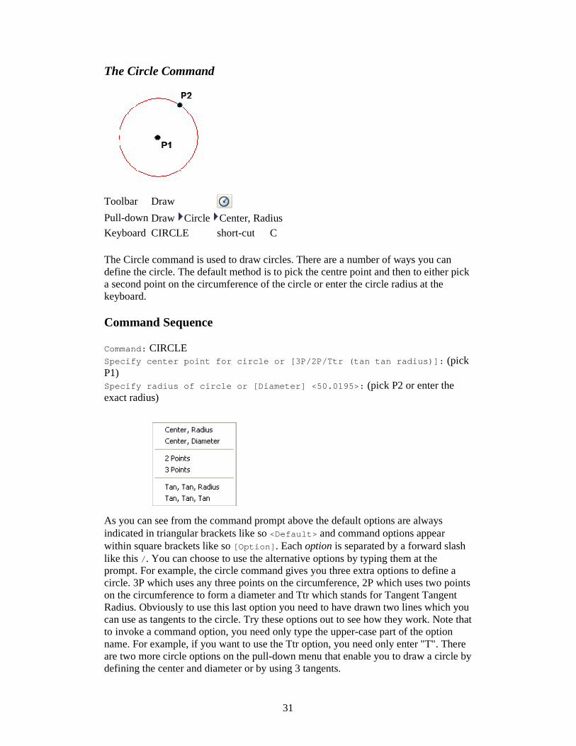
The Circle command is used to draw circles. There are a number of ways you can define the circle. The default method is to pick the centre point and then to either pick a second point on the circumference of the circle or enter the circle radius at the keyboard.

Command Sequence

Command: CIRCLE Specify center point for circle or [3P/2P/Ttr (tan tan radius)]: (pick P1) Specify radius of circle or [Diameter] <50.0195>: (pick P2 or enter the exact radius)

As you can see from the command prompt above the default options are always indicated in triangular brackets like so <Default> and command options appear within square brackets like so [Option]. Each option is separated by a forward slash like this /. You can choose to use the alternative options by typing them at the prompt. For example, the circle command gives you three extra options to define a circle. 3P which uses any three points on the circumference, 2P which uses two points on the circumference to form a diameter and Ttr which stands for Tangent Tangent Radius. Obviously to use this last option you need to have drawn two lines which you can use as tangents to the circle. Try these options out to see how they work. Note that to invoke a command option, you need only type the upper-case part of the option name. For example, if you want to use the Ttr option, you need only enter "T". There are two more circle options on the pull-down menu that enable you to draw a circle by defining the center and diameter or by using 3 tangents.

32

The Arc Command

Toolbar Draw Pull-down Draw Arc 3 Points

Keyboard ARC short-cut A

The Arc command allows you to draw an arc of a circle. There are numerous ways to define an arc, the default method uses three pick points, a start point, a second point and an end point. Using this method, the drawn arc will start at the first pick point, pass through the second point and end at the third point. Once you have mastered the default method try some of the others. You may, for example need to draw an arc with a specific radius. All of the Arc command options are available from the pull-down menu.

Command Sequence

Command: ARC Specify start point of arc or [Center]: (pick P1) Specify second point of arc or [Center/End]: (pick P2) Specify end point of arc: (pick P3)

It is also possible to create an arc by trimming a circle object. In practice, many arcs are actually created this way. See the Trim command on the Modifying Objects tutorial for details.

33

The Spline Command

Toolbar Draw Pull-down Draw Spline Keyboard SPLINE short-cut SPL

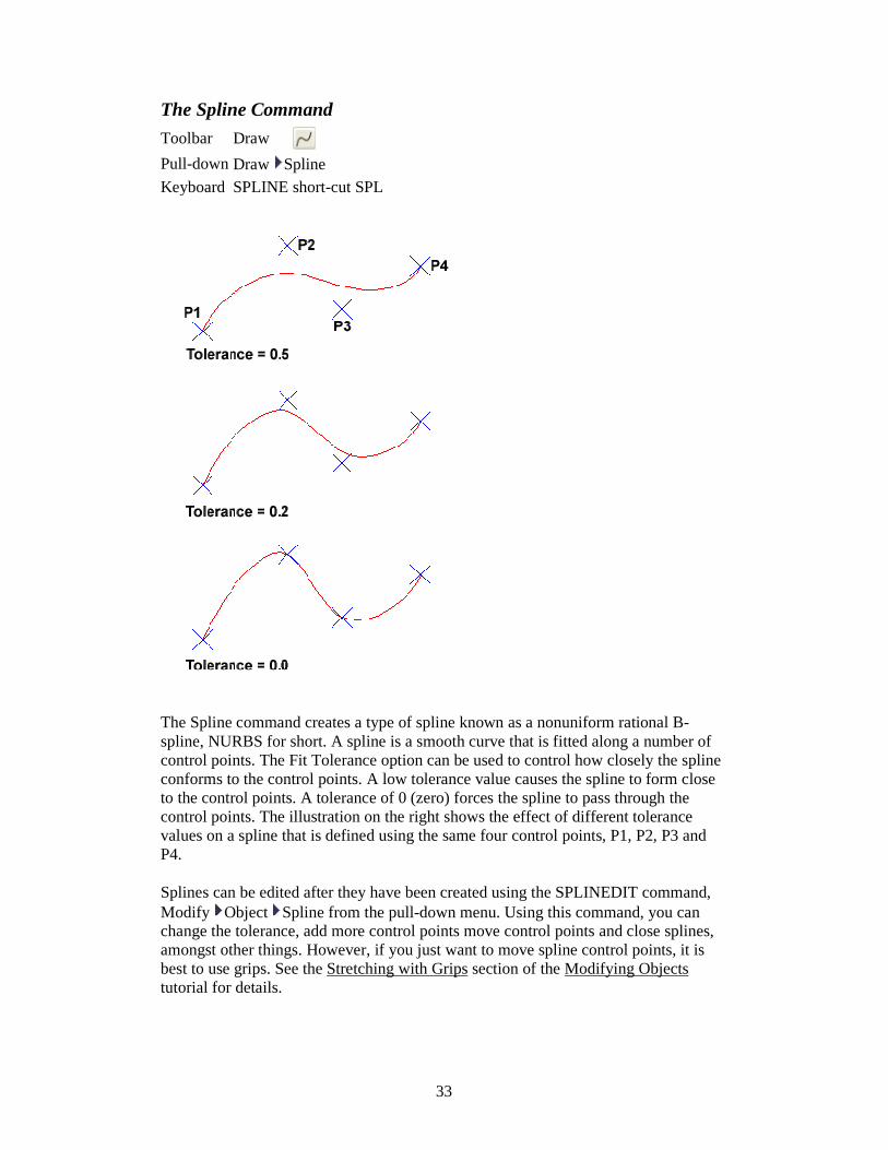
The Spline command creates a type of spline known as a nonuniform rational B-spline, NURBS for short. A spline is a smooth curve that is fitted along a number of control points. The Fit Tolerance option can be used to control how closely the spline conforms to the control points. A low tolerance value causes the spline to form close to the control points. A tolerance of 0 (zero) forces the spline to pass through the control points. The illustration on the right shows the effect of different tolerance values on a spline that is defined using the same four control points, P1, P2, P3 and P4.

Splines can be edited after they have been created using the SPLINEDIT command, Modify Object Spline from the pull-down menu. Using this command, you can change the tolerance, add more control points move control points and close splines, amongst other things. However, if you just want to move spline control points, it is best to use grips. See the Stretching with Grips section of the Modifying Objects tutorial for details.

34

Command Sequence

Command: SPLINE Specify first point or [Object]: (Pick P1) Specify next point: (Pick P2) Specify next point or [Close/Fit tolerance] <start tangent>: (Pick P3) Specify next point or [Close/Fit tolerance] <start tangent>: (Pick P4) Specify next point or [Close/Fit tolerance] <start tangent>: Specify start tangent: (pick a point) Specify end tangent: (pick a point)

You can create linear approximations to splines by smoothing polylines with the PEDIT command, Modify Polyline from the pull-down menu. However, you can also turn polylines into true splines using the Object option of the Spline command.

The Ellipse Command

Toolbar Draw Pull-down Draw Ellipse Axis, End Keyboard ELLIPSE short-cut EL

The Ellipse command gives you a number of different creation options. The default option is to pick the two end points of an axis and then a third point to define the eccentricity of the ellipse. After you have mastered the default option, try out the others.

Command Sequence

Command: ELLIPSE Specify axis endpoint of ellipse or [Arc/Center]: (pick P1) Specify other endpoint of axis: (pick P2) Specify distance to other axis or [Rotation]: (pick P3)

The ellipse command can also be used to draw isometric circles. See the worked example in the Drawing Aids tutorial to find out how to do this and how to draw in isometric projection with AutoCAD.

35

The Ellipse Arc Command

Toolbar Draw Pull-down Draw Ellipse Arc Keyboard ELLIPSE A short-cut EL A

The Ellipse Arc command is very similar to the Ellipse command, described above. The only difference is that, in addition to specifying the two axis end points and the "distance to other axis" point, you are prompted for a start and end angle for the arc. You may specify angles by picking points or by entering values at the command prompt. Remember that angles are measured in an anti-clockwise direction, starting at the 3 o'clock position.

In truth, the Ellipse Arc command is not a new or separate command; it is just an option of the Ellipse command and it therefore has no unique command line name. It is curious why Autodesk considered this option important enough to give it it's own button on the Draw toolbar. Still, there it is.

Command Sequence

Command: ELLIPSE Specify axis endpoint of ellipse or [Arc/Center]: A Specify axis endpoint of elliptical arc or [Center]: (pick P1) Specify other endpoint of axis: (pick P2) Specify distance to other axis or [Rotation]: (pick P3) Specify start angle or [Parameter]: 270 Specify end angle or [Parameter/Included angle]: 90

36

The Region Command

Toolbar Draw Pull-down Draw Region Keyboard REGION short-cut REG

A region is a surface created from objects that form a closed shape, known as a loop. The Region command is used to transform objects into regions rather than actually drawing them (i.e. you will need to draw the closed shape or loop first). Once a region is created, there may be little visual difference to the drawing. However, if you set the shade mode to "Flat Shaded", ViewShade Flat Shaded, you will see that the region is, in fact, a surface and not simply an outline. Regions are particularly useful in 3D

modeling because they can be extruded.

Before starting the Region command, draw a closed shape such as a rectangle, circle or any closed polyline or spline.

Command Sequence

Command: REGION Select objects: (Pick P1) Select objects: 1 loop extracted. 1 Region created.

You can use the boolean commands, Union, Subtract and Intersect to create complex regions.

37

WEEK 6

The Wipeout Command

Toolbar Custom Pull-down Draw Wipeout

Keyboard WIPEOUT

A Wipeout is an image type object. Most commonly it is used to "mask" part of a drawing for clarity. For example, you may want to add text to a complicated part of a drawing. A Wipeout could be used to mask an area behind some text so that the text can easily be read, as in the example shown on the right.

The Wipeout command can be used for 3 different operations. It can be used to draw a wipeout object, as you might expect, but it can also be used to convert an existing closed polyline into a wipeout and it can be used to control the visibility of wipeout frames.

Command Sequence

Command: WIPEOUT Specify first point or [Frames/Polyline] <Polyline>: (Pick P1)

Specify next point: (Pick P2) Specify next point or [Undo]: (Pick P3) Specify next point or [Close/Undo]: (Pick P4) Specify next point or [Close/Undo]:

You can use as many points as you wish in order to create the shape you need. When you have picked the last point, use right-click and Enter (or hit the Enter key on the keyboard) to complete the command and create the wipeout.

38

You may find that it is easier to draw a polyline first and then convert that polyline into a wipeout. To do this, start the Wipeout command and then Enter to select the default "Polyline" option. Select the polyline when prompted to do so. Remember, polylines must be closed before they can be converted to wipeouts.

In most cases, you will probably want to turn off the wipeout frame.

Command Sequence

Specify first point or [Frames/Polyline] <Polyline>: F (the Frames option) Enter mode [ON/OFF] <ON>: OFF

Regenerating model.

The Frames option is used to turn frames off (or on) for all wipeouts in the current drawing. You cannot control the visibility of wipeout frames individually. You should also be aware that when frames are turned off, wipeouts cannot be selected. If you need to move or modify a wipeout, you need to have frames turned on.

It is often more convenient to draw the wipeout after the text so that you can see how much space you need. In such a case, you may need to use the DRAWORDER command (Tools Display Order Option) to force the text to appear above the wipeout.

Tip: If you have the Express Tools loaded, you can use the very useful TEXTMASK command, which automatically creates a wipeout below any selected text. Find it on your pull-down at ExpressText Text Mask

Points and Point Styles

Points are very simple objects and the process of creating them is also very simple. Points are rarely used as drawing components although there is no reason why they could not be. They are normally used just as drawing aids in a similar way that

39

Construction Lines and Rays are used. For example, points are automatically created when you use the Measure and Divide commands to set out distances along a line.

When adding points to a drawing it is usually desirable to set the point style first because the default style can be difficult to see.

The Point Command

Toolbar Draw Pull-down Draw Point Single Point Keyboard POINT short-cut PO

The point command will insert a point marker in your drawing at a position which you pick in the drawing window or at any co-ordinate location which you enter at the keyboard. The default point style is a simple dot, which is often difficult to see but you can change the point style to something more easily visible or elaborate using the point style dialogue box. Points can be used for "setting out" a drawing in addition to construction lines. You can Snap to points using the Node object snap. See the Object Snap tutorial for details.

Command Sequence

Command: POINT Current point modes: PDMODE=0 PDSIZE=0.0000 Specify a point: (pick any point)

Strangely, in Multiple Point mode (the default for the Point button on the Draw toolbar) you will need to use the escape key (Esc) on your keyboard to end the command. The usual right-click or enter doesn't work.

The Point Style Command

Toolbar None

Pull-down Format Point Style…

Keyboard DDPTYPE

40

You can start the point style command from the keyboard by typing DDPTYPE or you can start it from the pull-down menu at FormatPoint Style… The command starts by displaying a dialogue box offering a number of options.

To change the point style, just pick the picture of the style you want and then click the "OK" button. You will need to use the Regen command, REGEN at the keyboard or View Regen from the pull-down to force any existing points in your drawing to display in the new style. Any new points created after the style has been set will automatically display in the new style.

One interesting aspect of points is that their size can be set to an absolute value or relative to the screen size, expressed as a percentage. The default is for points to display relative to the screen size, which is very useful because it means that points will remain the same size, irrespective of zoom factor. This is particularly convenient when drawings become complex and the drawing process requires a lot of zooming in and out.

Multilines

Multilines are complex lines that consist of between 1 and 16 parallel lines, known as elements. The default multiline style has just two elements but you can create additional styles of an almost endless variety. The Multiline Style command enables you to create new multiline styles by adding line elements, changing the colour and linetype of elements, adding end caps and the option of displaying as a solid colour.

41

The Multiline Command

Toolbar custom Pull-down Draw Multiline Keyboard MLINE short-cut ML

The Multiline command is used to draw multilines. This process of drawing is pretty much the same as drawing polylines, additional line segments are added to the multiline as points are picked. As with polylines, points can be unpicked with the Undo option and multilines can be closed.

When you start the Multiline command you also have the option to specify the Justification, Scale and Style of the multiline. The Justification option allows you to set the justification to "Top", the default, "Zero" or "Bottom". When justification is set to top, the top of the multiline is drawn through the pick points, as in the illustration below. Zero justification draws the centreline of the multiline through the pick points and Bottom draws the bottom line through the pick points. Justification allows you to control how the multiline is drawn relative to your setting out information. For example, if you are drawing a new road with reference to its centre line, then Zero justification would be appropriate.

The Scale option allows you to set a scale factor, which effectively changes the width of the multiline. The default scale factor is set to 1.0 so to half the width of the multiline, a value of 0.5 would be entered. A value of 2.0 would double the width.

The Style option enables you to set the current multiline style. The default style is called "Standard". This is the only style available unless you have previously created a new style with the Multiline Style command. Follow the command sequence below to see how the Multiline command works and then try changing the Justification and Scale options.

Command Sequence

Command: MLINE Current settings: Justification = Top, Scale = 20.00, Style = STANDARD Specify start point or [Justification/Scale/STyle]: (Pick P1) Specify next point: (Pick P2) Specify next point or [Undo]: (Pick P3)

42

Specify next point or [Close/Undo]: (to end or continue picking or C to close)

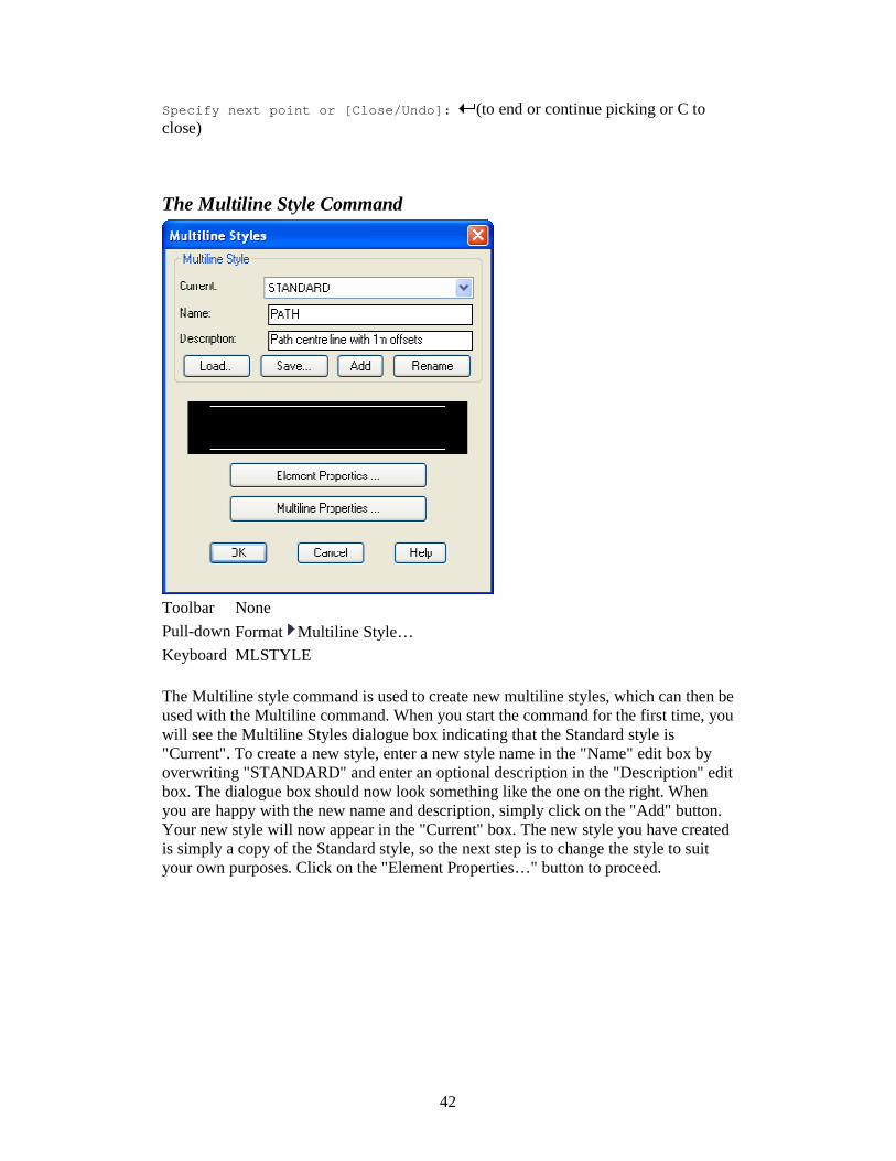
The Multiline Style Command

Toolbar None

Pull-down Format Multiline Style… Keyboard MLSTYLE

The Multiline style command is used to create new multiline styles, which can then be used with the Multiline command. When you start the command for the first time, you will see the Multiline Styles dialogue box indicating that the Standard style is "Current". To create a new style, enter a new style name in the "Name" edit box by overwriting "STANDARD" and enter an optional description in the "Description" edit box. The dialogue box should now look something like the one on the right. When you are happy with the new name and description, simply click on the "Add" button. Your new style will now appear in the "Current" box. The new style you have created is simply a copy of the Standard style, so the next step is to change the style to suit your own purposes. Click on the "Element Properties…" button to proceed.

43

You will now see the Element Properties dialogue box appear. This dialogue box allows you to add new line elements or delete existing ones and to control the element offset, colour and linetype. Click the "Add" button to add a new element. A new line element now appears with an offset of 0.0, in other words, this is a centre line. Highlight the top element in the "Elements" list and change the offset to 1.0 by entering this value in the "Offset" edit box. Now do the same with the bottom element remembering to enter a value of -1.0 because this is a negative offset. You now have a multiline that is 2 drawing units wide with a centre line. Let's now change the colour and linetype of the centre line.

Highlight the 0.0 offset element by clicking it in the "Elements" list. To change the colour, simply click on the Colour… button and select an appropriate colour from the palette. When a colour has been selected, click the "OK" button on the palette to return to the Element Properties dialogue box.

Changing the linetype is a little more complicated because we will need to load the required linetype first. However, click on the "Linetype…" button to proceed.

44

The Select Linetype dialogue box appears with just a few solid linetypes listed, ByLayer, ByBlock and Continuous. Click on the "Load…" button. The Load or Reload Linetypes dialogue box now appears. Scroll down the list of linetypes until you find one called "Hidden". Highlight Hidden and then click the "OK" button. You will now see the Hidden linetype appear in the "Loaded linetypes" list in the Select Linetype dialogue box, which should now look similar to the one shown above. Finally, highlight Hidden and click the "OK" button. Your Element Properties dialogue box should now look similar to the one in the illustration above. To complete our new style, we will add some end caps and a solid fill. Click on the "Multiline Properties…" button to proceed.

In the Multiline Properties dialogue box, click in the "Line" check boxes under "Start" and "End". This will have the effect of capping the ends of the multiline with a 90 degree line. As you can see from the dialogue box, you can change this angle if you wish to give a chamfered end. Next, click the "On" check box in the "Fill" section and then click on the Colour… button and select the fill colour from the palette. The Multiline Properties dialogue box should now look like the one in the illustration on the left. Finally, click the "OK" button in the Multiline Properties dialogue box and again in the Multiline Style dialogue box. You are now ready to draw with your new multiline.

Start the Multiline command, pick a number of points and admire your handiwork. If you have followed this tutorial closely, your new multiline should look something like the one in the illustration on the right. Notice the effect of the various changes you have made compared with the Standard multiline style.

45

One limitation of multiline styles is that you cannot modify a style if there are multilines referencing the style in the current drawing. This is a shame because it means that it is not possible to update multiline styles in the same way as it is possible to update text or dimension styles. You also cannot change the style of an existing multiline. If you really want to modify a multiline style, you will have to erase all multilines that reference the style first.

If you are new to AutoCAD, the whole process of working with multilines and creating multiline styles may appear a little bewildering because it touches upon a number of aspects of the program with which you may not be familiar. If this is the case, it may be a good idea to return to this tutorial in the future. Multilines are useful because they can save lots of time but their use is fairly specific and you should think carefully before using them. It may, for example, be more convenient simply to draw a polyline and to create offsets using the Offset command.

Tips & Tricks

• You will have noticed that many of the draw commands require the key on the keyboard to be pressed to end them. In AutoCAD, clicking the right mouse key and selecting "Enter" from the context menu has the same effect as using the key on the keyboard. Using the right-click context menu is a much more efficient way of working than using the keyboard.

• You can also use the key or right mouse click to repeat the last command used. When a command has ended, you can start it again by right clicking and selecting "Repeat command" from the context menu rather that entering the command at the keyboard or selecting it from the pull-down or toolbar. By this method it is possible, for example, to repeat the line command without specifically invoking it. The command sequence might be something like the one below.

Command Sequence

Command: LINE Specify first point: (pick P1) Specify next point or [Undo]: (pick P2)

46

Specify next point or [Undo]: (right-click and select Enter) Command: (right-click and select Repeat Line) Specify first point: (pick P1) Specify next point or [Undo]: (pick P2) Specify next point or [Undo]: (right-click and select Enter) Command: (right-click and select Repeat Line)…

You could continue this cycle as long as you needed, using only the mouse for input.

• You can change the Linetype of any of the objects created in the above tutorial. By default all lines are drawn with a linetype called "Continuous". This displays as a solid line. However, lines can be displayed with a dash, dash-dot and a whole range of variations. See the Object Properties tutorial for details.

47

WEEK 7

Object Selection In AutoCAD Introduction

Before you start to use the AutoCAD Modify commands, you need to know something about selecting objects. All of the Modify commands require that you make one or more object selections. AutoCAD has a whole range of tools which are designed to help you select just the objects you need. This tutorial is designed to demonstrate the use of many of the selection options. As with so many aspects of AutoCAD, developing a good working knowledge of these options can drastically improve your drawing speed and efficiency.

Selecting Objects by Picking

Perhaps the most obvious way to select an object in AutoCAD is simply to pick it. Those of you who have used other graphics based utilities will be familiar with this concept. Generally all you have to do is place your cursor over an object, click the mouse button and the object will be selected. In this respect AutoCAD is no different from any other graphics utility.

When you start a Modify command such as ERASE, two things happen. First, the cursor changes from the usual crosshairs to the pickbox and second, you will the the "Select objects" prompt on the command line. Both of these cues are to let you know that AutoCAD is expecting you to select one or more objects.

Select objects:

To select an object, place the pickbox over a part of the object and left-click the mouse. When the object has been picked it is highlighted in a dashed line to show that it is part of the current selection and the command line reports "1 found". You will now see the "Select objects" prompt on the command line again. At this point you can continue adding more objects to the current selection by picking them or you can press or the Space Bar to complete the selection.

48

The Crosshairs The Pickbox Highlighted Object

When you pick one or more objects in response to the "Select objects" prompt, you are effectively creating a selection set. Selection sets are an important concept in AutoCAD because they can be used to great effect, especially when drawings become large or complicated.

An Example

Follow the example below to get an idea how a selection set can be created by picking objects.

Draw Two Circles

Draw two circles using the CIRCLE command, DrawCircle Center, Radius from

the pull-down menu or from the Draw toolbar. The size and position of the circles does not matter.

Command: CIRCLE Specify center point for circle or [3P/2P/Ttr (tan tan radius)]: (pick a point in the middle of the drawing window) Specify radius of circle or [Diameter] <8.3453>: (pick another point to define the circle circumference) Command: CIRCLE Specify center point for circle or [3P/2P/Ttr (tan tan radius)]: (pick the center point of the second circle) Specify radius of circle or [Diameter] <37.9174>: (pick another point to define the circle circumference)

Erase the Two Circles

Erase the two circles using the ERASE command, Modify Erase from the pull-down

or from the Modify toolbar.

Command: ERASE Select objects: (place the pickbox over a circle circumference and left-click) 1 found Select objects: (place the pickbox over the second circle circumference and left-click) 1 found Select objects: (press to complete the selection and erase the objects)

Creating selection sets by picking objects can become quite tedious if you want to select a large number of objects. Just imagine having to pick a hundred or more

49

objects in a large drawing! Fortunately AutoCAD provides a number of selection options which can help you select objects more efficiently.

Window Selection

The Window option is invoked by typing W in response to the "Select objects" prompt. Window allows you to define a rectangle using two points in exactly the same way as the RECTANGLE command. Once the window is defined, all objects which lie entirely within the window will be selected.

The Window selection box is shown as a rectangle with a solid line

Only objects entirely within the window will be selected

Command Sequence

Command: (start one of the Modify commands such as ERASE) Select objects: W First corner: (pick first corner) Specify opposite corner: (pick second corner) Select objects: (at this point you can either select more objects or to complete the selection set and continue with the current command.)

Crossing Window Selection

The Crossing Window option is invoked by typing C at the "Select objects" prompt and is a variation of the Window command. The command sequence is exactly the same but objects are selected which lie entirely within the window and those which cross the window border.

50

The Crossing selection box is shown as a rectangle with a broken line

Objects within and crossing the window will be selected

Implied Windowing

Although you can explicitly invoke the Window and Crossing Window selection boxes by entering W or C at the keyboard when prompted to "Select objects", in practice this is rarely done. Both of these selection options are so commonly used that AutoCAD provides a method of implied windowing so that you don't have to use the keyboard at all. You can test this out without using any command. If you pick a point in space on the graphic window, you will notice that AutoCAD automatically assumes that you want to define a selection window and uses the pick point as the first point of that window. If you move the cursor to the right of the pick point you will get a Window selection box (solid line). If you move the cursor th the left you will get a Crossing Window selection box (broken line). With a little bit of practice the use of implied windowing can make the whole drawing process very efficient and you will rarely find yourself having to explicitly invoke the window selection options from the keyboard.

The Undo option

It often happens that you inadvertently add objects which you don't want to a selection set during its compilation. When this occurs in the middle of a complicated selection it can be pretty annoying. Fortunately AutoCAD allows you to undo the last selection made during the compilation of a selection set. All you need do is enter U at the next "Select objects" prompt to remove the objects previously added.

Selecting All Objects

The All option is invoked by typing ALL at the "Select objects" prompt. You can use this option to select all the objects in the current drawing, no picking is required. Objects on Locked or Frozen layers are not selected but objects on layers which are simply turned off are selected.

51

WEEK 8

Fence Selection

The Fence option allows you to draw a multi-segment line, like a Polyline. All objects which cross the fence will be selected. The Fence option is invoked by typing F at the "Select objects" prompt.

Command: (start one of the Modify commands such as ERASE)

Command Sequence

Select objects: F First fence point: (pick first point) Specify endpoint of line or [Undo]: (pick second point) Specify endpoint of line or [Undo]: (pick another point or to end fence selection) Select objects: ( to complete the selection set or add more objects)

Window Polygon Selection

The Window Polygon option, invoked by typing WP is similar to the Window option except that you can define an irregular polygon shape within which objects will be

52

selected. As with the Window option, only objects which fall entirely within the polygon will be selected.

Command Sequence

Command: (start one of the Modify commands) Select objects: WP First polygon point: (pick first point) Specify endpoint of line or [Undo]: (pick second point) Specify endpoint of line or [Undo]: (pick third point) Specify endpoint of line or [Undo]: (pick another point or to end polygon selection) Select objects: ( to complete the selection set or add more objects)

A polygon is formed by picking at least three points.

Crossing Polygon Selection

The Crossing Polygon option can be used in exactly the same way as the Window Polygon option but it has the same selection criteria as the Crossing Window option, i.e. objects will be selected if they fall entirely within or touch the polygon boundary. This option is invoked by typing CP at the "Select objects" prompt.

Note: Lines, polygons and windows drawn using the selection options do not exist as drawing objects. Once the selection has been made they disappear.

Using a Previous Selection

AutoCAD always remembers the last selection set you defined. This is very useful because you may need to make a number of changes using different commands to the same group of objects. In order to re-select the last selection set you can use the Previous option. The previous option is invoked by typing P at the "Select objects" prompt.

Selecting the Last Object

You can select the last object created by entering L at the "Select objects" prompt.

53

Object Cycling

When drawings become complicated it is sometimes difficult to select the particular object you want because it is either very close to or overlies another object. In such a case it may happen that the other object is selected and not the one you want. Object cycling is designed to overcome this problem. If you make a pick whilst holding the Control (Ctrl) key down, AutoCAD will respond with "<Cycle on>". If you continue to pick, each object near the pick point is highlighted in rotation. Just keep picking until the object you want is highlighted, then right-click or , AutoCAD responds "<Cycle off>", the required object is added to the selection set and you can continue to select more objects as normal.

Adding and Removing Objects

AutoCAD provides two methods for adding and removing objects to and from a selection set. As you know, objects can be added to a selection set simply by picking them or by using one of the methods outlined above. You can remove selected objects from a selection set just as easily by shift picking. If you hold the Shift key down on the keyboard while picking a selected object, that object will be deselected (removed from the current selection set). You can tell when a selected object has been deselected because it is no longer highlighted. You can remove more than one object at a time by holding down the Shift key while using implied windowing. However, none of the other selection options which require keyboard input will work using the shift pick method.

If you need to remove a more complex selection from the current selection set you should use the Remove option to switch to Remove mode. If you enter R at the "Select objects" prompt, AutoCAD will respond:

Remove objects:

Objects now picked or selected using any of the above methods will be removed from the current selection set. When you have finished removing objects, you can return to Add mode by entering A at the "Remove objects" prompt.

You can use any combination of picking, selection options and add/remove modes to define your selection set. Once you are happy that you have selected all the objects you need, just hit to complete the selection process and to continue with the current command.

When you feel confident with the basic selection tools, have a look at the Advanced Selection tutorial to find out how to use AutoCAD's advanced selection tools for creating complex selection sets.

54

WEEK 9

Modifying Objects Introduction

AutoCAD drawings are rarely completed simply by drawing lines, circles etc. Most likely you will need to Modify these basic drawing objects in some way in order to create the image you need. AutoCAD provides a whole range of modify tools such as Move, Copy, Rotate and Mirror. As you can see, the command names are easily understandable. However, the way these commands work is not always obvious. This tutorial is designed to show you how all of the Modify commands work. If you just need information quickly, use the QuickFind toolbar below to go straight to the information you need or select a topic from the contents list above.

As is usual with AutoCAD, the Modify tools can be accessed in one of three ways, from the keyboard, from the pull-down menu and from the toolbar. All of the Modify tools are available from the Modify pull-down and the Modify toolbar. In each section below, the toolbar, pull-down and keyboard options are given. The method you choose is entirely up to you. Ultimately you will use the method that you feel most comfortable with or the one you find most efficient. AutoCAD allows great flexibility and there aren't any right or wrong ways of working. That said, it should be pointed out that the use of toolbars in AutoCAD is almost always quicker than any other method.

55

The Modify toolbar is usually displayed by default but if it is not already displayed, you can display it using the TOOLBAR command, ViewToolbars… from the pull-down menu. When the Toolbar dialogue box (shown above) appears, simply check the box next to "Modify" in the toolbars list. Many AutoCAD users work with the Modify toolbar permanently docked on their screen because it gives one-click access to all of the commands, making the drawing process much more efficient.

The Erase Command

Toolbar Modify Pull-down Modify Erase Keyboard ERASE short-cut E

The Erase command is one of the simplest AutoCAD commands and is one of the most used. The command erases (deletes) any selected object(s) from the drawing.

Remember you can always get deleted objects back by typing U to undo, from the Standard toolbar or by using the OOPS command.

Command Sequence

Command: ERASE Select objects: (pick an object to erase) Select objects: (to end the selection and erase the object)

If you simply want to erase the last object you created you can type L at the "Select objects" prompt. The last object will be highlighted and you can then select more

56

objects or to end the command. See the "Object Selection" tutorial for more information on selecting objects.

The Copy Command

Toolbar Modify Pull-down Modify Copy Keyboard COPY short-cut CP

The Copy command can be used to create one or more duplicates of any drawing object or objects which you have previously created. Copy is a very useful and time-saving command because you can create very complex drawing elements and then simply copy them as many times as you like.

Command Sequence

Command: COPY Select objects: (pick object to copy, P1) Select objects: (to end selection) Specify base point or displacement, or [Multiple]: (pick P2 or M for multiple copies) Specify second point of displacement or <use first point as

displacement>: (pick P3)

The multiple option allows you to create additional copies of the selected object(s) by picking as many new points as you like. To end a multiple copy, just hit the key.

Notice that the "Base point", P2 and the "Second point", P3 do not have to be picked on or near the object. The two points are simply used to indicate the distance and direction of the copied object from the original object.

The Mirror Command

Toolbar Modify Pull-down Modify Mirror Keyboard MIRROR short-cut MI

57

The Mirror command allows you to mirror selected objects in your drawing by picking them and then defining the position of an imaginary mirror line using two points.

Command Sequence

Command: MIRROR Select objects: (pick object to mirror, P1) Select objects: (to end selection) Specify first point of mirror line: (pick P2) Specify second point of mirror line: (pick P3) Delete source objects? [Yes/No] <N>: (for No to keep the original object)

Notice that in the command sequence above, pressing the key when asked whether to "Delete source objects?" resulted in a "No" response. This is because "No" is the default option. AutoCAD always shows the default option within triangular brackets, in this case "<N>". Many AutoCAD commands offer default options. They are usually the most commonly used and you need only right-click and select "Enter" from the menu or press on the keyboard to accept them.

In order to create perfectly horizontal or vertical mirror lines use Ortho. For more information on the use of Ortho and other drawing aids, see the "Drawing Aids" tutorial.

The Offset Command

Toolbar Modify Pull-down Modify Offset Keyboard OFFSET short-cut O

Offset is probably one of the most useful commands for constructing drawings. The Offset command creates a new object parallel to or concentric with a selected object. The new object is drawn at a user defined distance (the offset) from the original and in a direction chosen by the user with a pick point. You can offset lines, arcs, circles, ellipses, 2D polylines, xlines, rays and planar splines.

58

Command Sequence

Command: OFFSET Specify offset distance or [Through] <1.0000>: 10 (specify distance) Select object to offset or <exit>: (select object, P1) Specify point on side to offset: (pick direction, P2) Select object to offset or <exit>: (to end or select another object to offset)

In the illustration below, a line (cyan) has been offset to the right through a distance "Offset" by picking a point to the right of the original line. The result is a new line (red) to the right of the original.

Circles can be offset inside or outside of themselves to create a new circle which is concentric (has the same centre point) with the original circle. In the illustration, a new circle (red) has been created outside of the original by picking a point outside of the original circle. The radius of the new circle is the offset distance "Offset" plus the radius of the original circle.

In the illustration above, the new objects and original objects are shown in different colours for clarity. In reality, offset objects inherit their object properties from the original object. See the "Object Properties" tutorial for details.

The Array Command

Toolbar Modify Pull-down Modify Array Keyboard ARRAY short-cut AR

The Array command makes multiple copies of selected objects in a rectangular matrix (columns and rows) or a polar (circular) pattern. This command has been completely transformed in AutoCAD 2000i. It is now completely dialogue box driven with the option to see a preview of the array before it is created. You can also now create rectangular arrays at a user specified angle. This constitutes a major improvement in usability.

59

WEEK 10

The Rectangular Array

The illustration on the right shows the results of a rectangular array with two columns an three rows. The distance between rows is indicated with the dimension DR and between columns with DC. When creating rectangular arrays it is important to remember that new rows are created above the original object and new columns are created to the right of the original object. The resulting array is, therefore, always created with the original object in the bottom left hand position with respect to the current co-ordinate system. In the illustration, the original object is shown in cyan and the new objects in red. It is possible to create arrays which do not align with the World Co-ordinate System by setting a User Co-ordinate System first. See the UCS tutorial for details.

Try creating this array yourself. First, draw a rectangle 20 drawing units wide and 10 drawing units tall. To do this, start the rectangle command Draw Rectangle from the pull-down menu. When you are prompted to pick a point, pick somewhere in the lower left quarter of the drawing area. Then, when you are prompted for a second point, enter the relative cartesian co-ordinate @20,10. You have now drawn a rectangle at the right size. See the Using Co-ordinates tutorial for more information on drawing with co-ordinates.

60

Now start the Array command.First of all, make sure that the Rectangular Array radio button is selected and that you are looking at the Rectangular Array dialogue box and now follow the steps below:

1. Click the Select objects button. The dialogue box will temporarily disappear enabling you to select the rectangle you just drew. Press the Return button on your keyboard to complete the selection. You are now returned to the dialogue box and the message immediately below the Select Objects button should read "1 objects selected".

2. Enter the number of rows required in the Rows edit box. For this example, enter the value "3". Notice that the schematic preview on the right hand side of the dialogue box updates to reflect the values you are entering.

3. Enter the number of columns required in the Columns edit box. Enter the value "2".

4. Enter the row offset in the Row Offset edit box. This is the distance DR in the illustration above. Note that tis is not the distance between rows. In this example, our rectangle is 10 units high and we will enter a row offset of 15. The result will be a 5 unit gap between rectangles.

5. Enter the column offset in the Column Offset edit box. The same parameters apply as for the row offset. Enter a value of 25 to give a 5 unit gap between our rectangles.

6. Click on the Preview button. Once again, the dialogue box disappears and the specified array is temporarily drawn so that we can preview it. We are now offered 3 choices. If the array isn't quite right, click the Modify button to

61

return to the Array dialogue box. If you are happy with the array, click the Accept button, the array will be permanently drawn and the command is ended.

You should now have an array that looks similar to the one in the illustration above consisting of 6 rectangles arranged in 3 rows and 2 columns. As you can se, this command is very powerful and can save lots of time if used carefully.

The Polar Array

The polar array works in a similar way to the rectangular array. The main difference is that rather than specifying the number and offset for rows and columns, you must specify a center point and the total number of objects in the array (including the original object).

You can try this for yourself by drawing another rectangle as described above. This time, though, locate the rectangle in the centre top half of the drawing area. Now, start the Array command, click the Polar Array radio button and follow the steps below:

1. Click the Select objects button. The dialogue box will temporarily disappear enabling you to select the rectangle you just drew. Press the Return button on your keyboard to complete the selection. You are now returned to the dialogue box and the message immediately below the Select Objects button should read "1 objects selected".

2. Specify the center point for the array. This is the point C in the illustration below. You can do this by entering x and y co-ordinates into the appropriate edit boxes if you know what these values should be. However, this is rarely the case and most often you will want to click the Pick Center Point button to

62

pick a point from the drawing area. Pick a point somewhere below the rectangle you have just drawn.

3. Enter a value for the total number of items. For this example, enter the value "6". Notice that once again, the schematic preview updates to reflect the values you have entered.

4. Make sure that the Rotate items as copied checkbox is checked.

5. Click on the Preview button. Once again, the dialogue box disappears and the specified array is temporarily drawn so that we can preview it. We are now offered 3 choices. If the array isn't quite right, click the Modify button to return to the Array dialogue box. If you are happy with the array, click the Accept button, the array will be permanently drawn and the command is ended.

The array you have just drawn should look something like the one illustrated below, left. Take some time to play around with the other options in the Array dialogue box to see what they can do.

The illustration above shows the results of a polar array using an original rectangle (cyan) copied six times about a centre point C, through an angle of 360 degrees (full circle). The only difference between the array on the left and the one on the right is that the Rotate items as copied checkbox was not checked in the right hand example.

All new objects created with the Array command will inherit the object properties of the original object. See the "Object Properties" tutorial for information on object properties.

The Move Command

Toolbar Modify Pull-down Modify Move

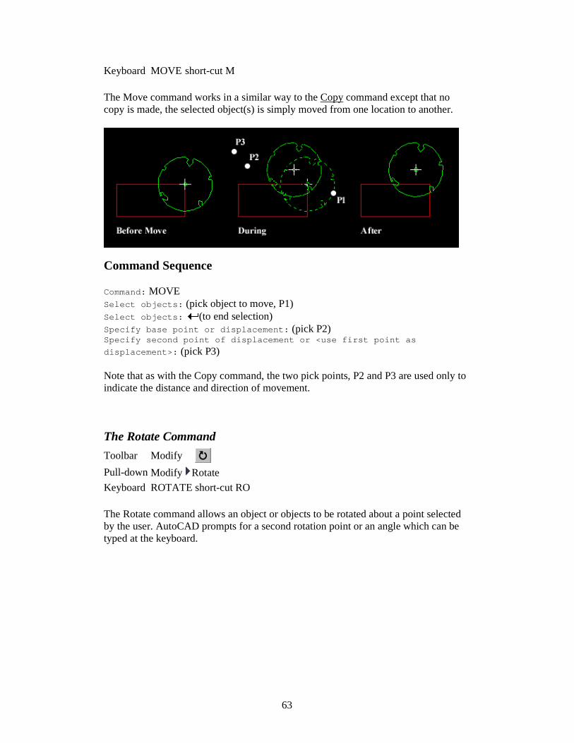
63

Keyboard MOVE short-cut M

The Move command works in a similar way to the Copy command except that no copy is made, the selected object(s) is simply moved from one location to another.

Command Sequence

Command: MOVE Select objects: (pick object to move, P1) Select objects: (to end selection) Specify base point or displacement: (pick P2) Specify second point of displacement or <use first point as

displacement>: (pick P3)

Note that as with the Copy command, the two pick points, P2 and P3 are used only to indicate the distance and direction of movement.

The Rotate Command

Toolbar Modify Pull-down Modify Rotate

Keyboard ROTATE short-cut RO

The Rotate command allows an object or objects to be rotated about a point selected by the user. AutoCAD prompts for a second rotation point or an angle which can be typed at the keyboard.

64

Command Sequence

Command: ROTATE Current positive angle in UCS: ANGDIR=counterclockwise ANGBASE=0 Select objects: (pick object to rotate, P1) Select objects: (to end selection) Specify base point: (pick base point, P2) Specify rotation angle or [Reference]: (pick second point, P3 or enter angle)

Remember, by default, AutoCAD angles start at 3 o'clock and increase in an anti-clockwise direction. The "ANGDIR" and "ANGBASE" variables remind you of this. If you want to rotate in a clockwise direction you can enter a negative angle by using a minus sign.

Note: You can change the angle direction and the base angle using the Units command, Format Units… from the pull-down menu. Click the "Clockwise" check box to change the direction and click the "Direction…" button to set the base angle.

The Scale Command

Toolbar Modify Pull-down Modify Scale

Keyboard SCALE short-cut SC

The Scale command can be used to change the size of an object or group of objects. You are prompted for a pick point about which the selection set will be scaled. Scaling can then be completed by picking a second point (not always easy because it can sometimes be difficult to precisely control the scaling) or by entering a scale factor at the keyboard. For example a scale factor of 2 will double the size of the objects in the selection set and a factor of 0.5 will half them.

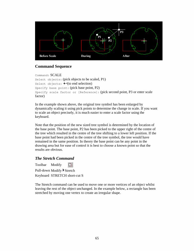
65

Command Sequence

Command: SCALE Select objects: (pick objects to be scaled, P1) Select objects: (to end selection) Specify base point: (pick base point, P2) Specify scale factor or [Reference]: (pick second point, P3 or enter scale factor)

In the example shown above, the original tree symbol has been enlarged by dynamically scaling it using pick points to determine the change in scale. If you want to scale an object precisely, it is much easier to enter a scale factor using the keyboard.

Note that the position of the new sized tree symbol is determined by the location of the base point. The base point, P2 has been picked to the upper right of the centre of the tree which resulted in the centre of the tree shifting to a lower left position. If the base point had been picked in the centre of the tree symbol, the tree would have remained in the same position. In theory the base point can be any point in the drawing area but for ease of control it is best to choose a known point so that the results are obvious.

The Stretch Command

Toolbar Modify Pull-down Modify Stretch Keyboard STRETCH short-cut S

The Stretch command can be used to move one or more vertices of an object whilst leaving the rest of the object unchanged. In the example below, a rectangle has been stretched by moving one vertex to create an irregular shape.

66

Command Sequence

Command: STRETCH Select objects to stretch by crossing-window or crossing-polygon... Select objects: (pick first point of crossing window) Specify opposite corner: (pick second point of window) Select objects: (to end selection) Specify base point or displacement: (pick base point) Specify second point of displacement: (pick second point)

To select vertices to stretch, you must use a crossing window or polygon. See the "Object Selection" tutorial for details of these selection methods.

Stretching with Grips

Although the Stretch command can be very useful, it has largely been superseded by the use of "Grips" which allow this sort of modification to be made much more intuitively.

To stretch an object using grips, simply select the object by clicking on it (you can do this without starting a command). The object becomes highlighted and small square grips appear at each vertex and various snap points, depending upon the object type. Click a grip to activate it and click again to reposition it. When you have completed your modifications, use the Escape key (Esc) at the top left of your keyboard to deselect the object and release grips.

The Lengthen Command

Toolbar Modify Pull-down Modify Lengthen

67

Keyboard LENGTHEN short-cut LEN

The Lengthen command can often be used instead of either the Trim or Extend commands. Indeed the end result is exactly the same. The Lengthen command can be used to either lengthen or shorten Lines, Arcs, open Polylines, elliptical Arcs and open Splines without the use of cutting or boundary edges.

Command Sequence

Command: LENGTHEN Select an object or [DElta/Percent/Total/DYnamic]: DY Select an object to change or [Undo]: (select a line or arc) Specify new end point: (pick new end point) Select an object to change or [Undo]: (to end)

The command sequence above demonstrates the use of the Dynamic Lengthen option which is probably the most useful for general purpose drafting. However, the other options are worth getting to know because they can save lots of time and effort.

The Total option allows you to change the total length of a line to any value that you specify. The Percent option allows you to change a line length using a percentage. For example, a value of 50 will result in a line one half the length of the original and a value of 200 will result in a line twice the length of the original. The Delta option can be used to extend or reduce the endpoint of a line by a given distance. The endpoint affected by the change is the one closest to the pick point when the object selection is made.

The Trim Command

Toolbar Modify Pull-down Modify Trim Keyboard TRIM short-cut TR

The Trim command can be used to trim a part of an object. In order to trim an object you must draw a second object which forms the "cutting edge". Cutting edges can be lines, xlines, rays, polylines, circles, arcs or ellipses. Blocks and text cannot be

68

trimmed or used as cutting edges. The illustration on the right shows the Trim command in action. The red square and circle have been drawn using the Polygon and Circle commands respectively. In order to trim these objects, a line has been drawn (cyan in the illustration), this forms the cutting edge. The Trim command, unlike most other modify commands requires that two separate object selections are made. The cutting edges are selected first (there can be one or more) and then the objects to be trimmed are selected. In the example above, the line is selected first because it forms the cutting edge and then the square and circle are selected.

The Trim command is slightly more complicated than many other modify commands. To get a better understanding of how it works, draw a square, circle and line as illustrated above and then follow the command sequence below. Don't forget to watch the AutoCAD command line at each stage of the process.

Command Sequence

Command: TRIM Current settings: Projection=UCS Edge=None Select cutting edges ... Select objects: (select the cutting edge, P1) Select objects: (to end cutting edge selection) Select object to trim or shift-select to extend or

[Project/Edge/Undo]:(pick the part of the square which you want to trim, P2) Select object to trim or shift-select to extend or

[Project/Edge/Undo]: (pick the circle, P3) Select object to trim or shift-select to extend or

[Project/Edge/Undo]: (to end)

Notice that at each trimming step you are given the option to undo the previous trim. This can be very useful if you inadvertently pick the wrong object.

In the above example, when the objects were trimmed, both pick points were made to the right of the cutting edge, resulting in the removal of that part of the objects to the right of the cutting edge. Obviously, the portion of square and circle to the left of the cutting edge could have been removed by picking to the left of the cutting edge. Also, you may not have noticed it, but by trimming a circle you have created an Arc object. This makes no visible difference but the object type has changed.

The Extend Command

Toolbar Modify Pull-down Modify Extend Keyboard EXTEND short-cut EX

69

This command extends a line, polyline or arc to meet another drawing object (known as the boundary edge). In the illustration on the right, two lines (red) are extended to meet another line (cyan) which forms the boundary edge. This command works in a similar way to the Trim command, described above. Two selections are made, one for the boundary edge(s) and one for the object(s) to extend.

Lines and other objects can be extended in one of two directions. In the illustration on the right, the red line could be extended either to the right or to the left. You can tell AutoCAD in which direction to extend by picking a point to the right or left of the midpoint respectively. AutoCAD does not intuitively know where the boundary edge lies so you must explicitly indicate the direction of extension by picking either one side or other of the midpoint.

Draw the lines as shown in the illustration and follow the command sequence below.

Command Sequence

Command: EXTEND Current settings: Projection=UCS Edge=None Select boundary edges ... Select objects: (select the boundary edge, P1) Select objects: (to end boundary edge selection) Select object to extend or shift-select to trim or

[Project/Edge/Undo]: (pick the object which you want to be extended, P2) Select object to extend or shift-select to trim or

[Project/Edge/Undo]: (pick another object which you want to be extended, P3) Select object to extend or shift-select to trim or

[Project/Edge/Undo]: (to end)

Sometimes you may get the message "Object does not intersect an edge" or "No edge in that direction". If this happens it means that you are either picking the wrong end of the object or the object you are trying to extend will not meet the boundary edge. The solution is either to pick near the end you want to extend or to move the boundary edge so that the extended line will intersect with it.

Using Edgemode

70

If the line you are trying to extend does not intersect with the boundary line, you can use the "Edge" option to toggle Edgemode to "Extend" (the default is "No Extend"). When the Extend command is set to Extend Mode, the objects being extended will extend to an imaginary line through the boundary edge, irrespective of whether the extended object actually intersects with the boundary edge. This is particularly useful and can save lots of time.

The illustration on the left shows the result of extending a line (red) to a boundary edge (cyan) with Edgemode set to "Extend". The same process would have resulted in an error message if Edgemode had been set to "No Extend". To get a better understanding of how this works, draw the two lines as shown in the illustration and try to extend them using the default settings. When you have done that, follow the command sequence below.

Command Sequence (Edgemode)

Command: EXTEND Select boundary edges: (Projmode = UCS, Edgemode = No extend) Select objects: (select the boundary edge, P1) Select objects: (to end boundary edge selection) Select object to extend or shift-select to trim or

[Project/Edge/Undo]: E (to use the Edge option) Enter an implied edge extension mode [Extend/No extend] <No extend>: E (to set Edgemode to Extend) Select object to extend or shift-select to trim or

[Project/Edge/Undo]: (pick the object to be extended, P2) Select object to extend or shift-select to trim or

[Project/Edge/Undo]: (to end)

Notice that the current value of Edgemode is always displayed on the command line when you start the Extend command. The Edge option can also be used with the Trim command to enable trimming to cutting edges which do not actually intersect the object to trim. Edgemode is a system variable, so any change to its value will affect both the Trim and Extend commands.

See the Lengthen command for more ways to extend and trim objects.

71

Shift Selection with Trim & Extend

You may have noticed during the command sequences for the Trim and Extend commands that you have the option to "shift-select". This feature is new to AutoCAD 2000i and it enables you to extend while using the Trim command and to trim while using the Extend command. These two commands are very closely related and you often need to trim and extend objects at the same time. If you are a beginner with AutoCAD it may be a good idea to avoid this feature initially, the Trim and Extend commands can be tricky to get to grips with in any case. However, do remember this feature because it is a great time saver.

The Break Command

Toolbar Modify Pull-down Modify Break Keyboard BREAK short-cut BR

The Break command enables you to break (remove part of) an object by defining two break points. In the illustration below, a corner of a rectangle has been removed. The Break command can be used with lines, polylines, circles, arcs ellipses, splines, xlines and rays. When you break an object, you can either select the object using the first break point and then pick the second break point, or you can select the object and then pick the two break points.

Command Sequence

Command: BREAK Select objects: (select the object using the first break point, P1) Specify second break point or [First point]: (pick the second break point, P2) The section of the object is removed and the command ends.

Sometimes you may want to select the object first and then specify the two break points. If this is the case, use the "First point" option to specify the first break point. By default, AutoCAD assumes that the point used to select the object is the first break point. This is often confusing for new users.

It may sometimes be necessary to break a line into two without removing any part of it. In this case, simply pick the first and second break points in the same position.

72

The Chamfer Command

Toolbar Modify Pull-down Modify Chamfer Keyboard CHAMFER short-cut CHA

The Chamfer command enables you to create a chamfer between any two non-parallel lines as in the illustration below or any two adjacent polyline segments. Usually, the Chamfer command is used to set the chamfer distances before drawing the chamfer. Follow the command sequence below where the chamfer distances are changed to 20 before the chamfer is made.

Command Sequence

Command: CHAMFER (TRIM mode) Current chamfer Dist1 = 10.0000, Dist2 = 10.0000 Select first line or [Polyline/Distance/Angle/Trim/Method]: D (to set distances) Specify first chamfer distance <10.0000>: 20 (enter required distance) Specify second chamfer distance <20.0000>: (first distance value or enter a different value) Select first line or [Polyline/Distance/Angle/Trim/Method]: (pick P1) Select second line: (pick P2) The chamfer is made and the command ends.

Notice from the command sequence that there are a number of options which can be used to control the way the Chamfer command behaves. The Polyline option can be used to chamfer all vertexes of a polyline simultaneously. The Distance option allows you to specify the two chamfer distances. Angle allows the angle between the first line and the chamfer to be specified. Trim is used to control whether the original lines are trimmed to the chamfer or remain as they are. Finally, Method is used to toggle the command between Distance and Angle mode. When Angle mode is used, the chamfer is defined using one distance and an angle rather than two distances.

The Fillet Command

Toolbar Modify Pull-down Modify Fillet

73

Keyboard FILLET short-cut F

The Fillet command is a very useful tool which allows you to draw an arc between two intersecting lines or adjacent polyline segments. You first need to use the command to set the required radius and then a second time to select the two lines.

Command Sequence

Command: FILLET Current settings: Mode = TRIM, Radius = 10.0000 Select first object or [Polyline/Radius/Trim]: R Specify fillet radius <10.000>: 25 Select first object or [Polyline/Radius/Trim]: (pick P1) Select second object : (pick P2)

The Fillet command can also be used to fillet arcs and circles. The "Polyline" option also allows you to fillet all vertices of a polyline with a single command. It's worth experimenting with this command, it can save you lots of time and enables you to construct shapes which otherwise would be quite difficult.

For example, you can easily create the lozenge shape shown on the right from a simple rectangle. Since AutoCAD rectangles are just closed polylines, you can use the Polyline option of the Fillet command to fillet all polyline vertexes simultaneously. Try this for yourself; draw a rectangle and then follow the command sequence below.

Command Sequence

Command: FILLET Current settings: Mode = TRIM, Radius = 10.0000 Select first object or [Polyline/Radius/Trim]: P Select 2D polyline: (pick P1) 4 lines were filleted

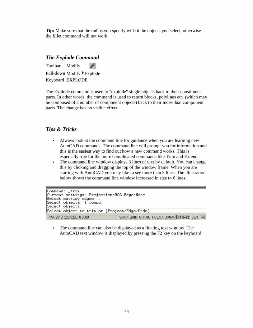
74

Tip: Make sure that the radius you specify will fit the objects you select, otherwise the fillet command will not work.

The Explode Command

Toolbar Modify Pull-down Modify Explode Keyboard EXPLODE

The Explode command is used to "explode" single objects back to their constituent parts. In other words, the command is used to return blocks, polylines etc. (which may be composed of a number of component objects) back to their individual component parts. The change has no visible effect.

Tips & Tricks

• Always look at the command line for guidance when you are learning new AutoCAD commands. The command line will prompt you for information and this is the easiest way to find out how a new command works. This is especially true for the more complicated commands like Trim and Extend.

• The command line window displays 3 lines of text by default. You can change this by clicking and dragging the top of the window frame. When you are starting with AutoCAD you may like to see more than 3 lines. The illustration below shows the command line window increased in size to 6 lines.

• The command line can also be displayed as a floating text window. The AutoCAD text window is displayed by pressing the F2 key on the keyboard.

75

WEEK 11

Direct Distance Entry

Introduction Direct distance entry is one of those AutoCAD features that is often overlooked. This is rather unfortunate because it can be extremely useful and an amazing time-saver. Basically, direct distance entry enables you to draw an object, such as a line, by pointing in a particular direction with the cursor and entering a distance at the command line.

How does it work? Say, for example, you wanted to draw a horizontal line with a length of 30 drawing

units. Start the Line command, DrawLine from the pull-down menu or from the Draw toolbar. When prompted, to specify the first point for the line, pick a point somewhere on the left side of the drawing area.

You now need to constrain the line to the horizontal. You can do this using Polar Tracking . Use the POLAR button on the status bar to turn on Polar Tracking. Usually, Polar Tracking is on by default, so you may not need to do this.

Now, move your cursor to the right of the first pick point. If you are within a few degrees of the horizontal, you should see something similar to the illustration on the right. Hold your cursor in this position and simply enter 30 at the keyboard. When you hit the Return key, a line segment is drawn, 30 units long and in the direction you were pointing.

Obviously, you could vary this sequence to get different effects. If you only want to draw horizontal or vertical lines, you could use Ortho rather than Polar Tracking. Or, you could configure polar tracking to snap to other angles like 45º or 30º. You might even want to turn both Ortho and Polar Tracking off and use free angles. See the Drawing Aids tutorial to learn more about Polar Tracking.

It's also worth pointing out that when Polar Tracking has snapped to an angle, as in the illustration above, a Tool Tip is displayed. This Tool Tip displays a relative polar co-ordinate from the first pick point to the current cursor position. The first number is the distance between the two points and it can be quite useful as a drawing guide since

76

the value updates dynamically. See the Using Co-ordinates tutorial for more information on polar co-ordinates.

Drawing Aids

Drawing with AutoCAD is really just like drawing on a drawing board. Most newcommers to Computer Aided Design assume that they will need to learn how to draw all over again. In fact, many of the drawing aids that AutoCAD provides are analagous to traditional drafting tools. Just as you have a parallel motion and set squares to help you draw horizontal and vertical lines on a drawing board, AutoCAD has similar drawing aids which can help you to draw horizontal and vertical lines on a computer. This means that in many respects, the drawing techniques are very similar. If you ever get stuck, think how you would complete a task on a drawing board and then look for a similar way to do it with AutoCAD.

Ortho Mode Status Bar Pull-down None Keyboard ORTHO or F8

Ortho is short for orthogonal, which means either vertical or horizontal. Like the other options on the status bar, Ortho is not really a command, it is a drawing mode which can either be turned on or off. Ortho mode can be toggled on or off in one of three ways. The quickest way is just to click on the ORTHO button on the status bar. The appearance of the button tells you whether Ortho is currently turned on or turned off. When Ortho is turned on, the ORTHO button appears pressed in. You can see how this appears by looking at the status bar illustration below. In the illustration, Ortho is turned on but Grid and Snap are turned off.

Ortho can also be toggled on and off using the F8 Function key (see Function Keys below for more details). Finally, you can also type ORTHO at the command prompt as in the command sequence below. Using Ortho is the equivalent of using your parallel motion and set square on a drawing board. With Ortho mode turned on you can only draw lines which are either vertical or horizontal. Turn Ortho mode on now and draw some lines to get a feeling for how it works.

77

Command Sequence

Command: ORTHO Enter mode [ON/OFF] <OFF>: (type ON or OFF)

Ortho mode is probably the simplest of all the drawing aids, and historically one of the oldest. It is either on or it is off and there are no special settings to make. Also, it does a very simple job; it constrains drawn lines to the horizontal or the vertical. You may not be surprised to learn, therefore, that its use has largely been superceded by more recent features, particularly Polar Tracking, described below.

The Drawing Grid Status Bar (right-click for settings) Pull-down None

Keyboard GRID or F7

The drawing grid is a regular pattern of dots displayed on the screen which acts as a visual aid, it is the equivalent of having a sheet of graph paper behind your drawing on a drawing board. You can control the grid spacing, so it can give you a general idea about the size of drawn objects. It can also be used to define the extent of your drawing. See, Setting Grid Limits, for more details.

Command Sequence

Command: GRID Specify grid spacing(X) or [ON/OFF/Snap/Aspect] <10.000>: (enter grid spacing)

Grid spacing set to 10 drawing units

Grid spacing set to 5 drawing units

Although you can use the command line to control the visibility of the grid by using the "ON" and "OFF" options this is more easily achieved using the F7 key or, better still, by clicking the GRID button on the status bar. However, the command line does offer some additional options. The Snap option allows you to automatically set the grid spacing to the current snap spacing (see Snap Mode below). You can also change

78

the aspect ration of the grid. By default, the X and Y spacing of the Grid are the same, resulting in a regular square matrix of grid points. But you can display a grid with different X and Y spacing by using the "Aspect" option.

Grid mode and X/Y spacing can also be set using the Drafting Settings dialogue box. You can access grid settings by right-clicking the Grid button on the status bar and selecting Settings… from the menu. You can also do this from the pull-down menu, Tools Drafting Settings… and click on the "Snap and Grid" tab.

You may have noticed that the grid does not extend infinitely in all directions. In fact, it is only displayed within a finite rectangle. You can control the extent of the visible grid using Drawing Limits.

Setting Grid Limits Toolbar None

Pull-down Format Drawing Limits

Keyboard LIMITS

Drawing Limits is used to define the extent of the grid display and to toggle Limits mode which can be used to define the extent of your drawing. The grid is displayed within a rectangle defined by two pick points or co-ordinates.

Command Sequence

Command: LIMITS Reset Model space limits: Specify lower left corner or [ON/OFF] <0.0000,0.0000>: (pick point, enter co-ordinates or to accept the default value) Specify upper right corner <420.0000,297.0000>: (pick point, enter co-ordinates or to accept the default value)

Drawing Limits can also be used to turn Limits mode on or off. Limits mode can be used to control where objects can and cannot be drawn. Limits is turned off by default which means that there is no restriction as to where points can be picked and objects drawn. When Limits is on, AutoCAD will not allow points to be picked or co-ordinates entered at the command line which fall outside of the specified drawing limits. If you try to pick a point outside the drawing limits when Limits mode is turned on, AutoCAD reports to the command line:

**Outside limits

79

Limits mode is useful if you know the extent of your plotted drawing sheet and you want to prevent objects being drawn outside of this area. However, Drawing Limits is most commonly used simply to control the extent of the Grid.

Snap Mode Status Bar (right-click for settings) Pull-down None

Keyboard SNAP or F9

Snap mode takes AutoCAD one step further than the drawing board. With Snap mode turned on AutoCAD only allows you to pick points which lie on a regular grid. The Snap grid is completely independent of the display grid. However, the Grid spacing and Snap spacing are usually set to the same value to avoid confusion. You can force the display grid to conform with the snap grid by setting the display grid spacing to zero. The display grid will then automatically change each time the snap grid is changed. When Snap mode is turned on and the Grid is displayed, the Snap and Grid spacings are the same and the crosshairs will jump from one grid point to another as you move across the screen. This makes it very easy to draw objects which have a regular shape. The Snap command is used to set the snap spacing and to toggle Snap mode.

Command Sequence

Command: SNAP Specify snap spacing or [ON/OFF/Aspect/Rotate/Style/Type] <10.0000>: (enter the required snap spacing in drawing units)

Orthographic Projection

80

Isometric Projection

Although you can use the Snap command to turn Snap mode on and off, it is much more efficient to use the F9 function key on the keyboard or to click the SNAP button on the status bar.

The "Aspect" option can be used to vary the horizontal and vertical snap spacings independently.

"Rotate" is used to set the snap grid to any angle.

You can also set the snap style to either Isometric or Standard (the default) using the "Style" option. The Standard style is used for almost all drawing situations including detail drawings in Orthographic Projection. The Isometric style is specifically to aid the creation of drawings in Isometric Projection (see the illustrations on the right).

The "Type" option allows you to set the snap type to either Grid (the default) or to Polar. The Polar option can be used in conjunction with Polar Tracking so that Snap mode snaps along polar tracking angles rather than to the grid.

The grid snap is particularly useful if you need lots of modular objects such as bricks or paviors. In the illustration on the left, the Aspect option is used to set the X and Y snap spacings to the brick dimensions and the Rotate option is used to set the orientation of the bond. Once these settings are made, the bricks can be accurately drawn without any other drawing aids.

81

All of the Snap variables can also be set using the Drafting Settings dialogue box. Right-click on the SNAP button and choose Settings… from the menu.

Drafting Settings Toolbar None

Pull-down Tools Drafting Settings… Keyboard DDRMODES

The Snap and Grid mode settings, can also be made from the Drafting Settings dialogue box, illustrated below .This dialogue can be invoked from the command line or from the pull-down menu but probably the simplest way is to right-click on either the GRID or SNAP buttons on the status bar and choose "Properties…" from the context menu. The advantage of the Drafting Settings dialogue box is that it gives you one-stop access to all the Grid and Snap settings.

These options act in the same way as those in the respective commands described above, see The Snap Command and The Grid Command for details. If you are creating drawings in isometric projection, use the "Isometric snap" option to change the grids from the standard orthogonal square grid to a 30 degree isometric grid.

82

Standard orthogonal grid Isometric grid

Polar Tracking Status Bar (right-click for settings)

Pull-down None Keyboard F10

Polar Tracking is a bit like Ortho mode on steroids. Whereas Ortho constrains your lines to either the horizontal or the vertical, Polar Tracking allows you to snap into whatever angles you choose to configure.

By default, Polar Tracking snaps only to the horizontal and the vertical. When you are drawing a line, pick the first point and then move the cursor close to a vertical or horizontal location and your cursor will snap into place. You will see a polar tracking vector and a tool tip which displays the angle and the distance from the pick point; in other words, a relative polar co-ordinate.

83

In this default setting, Polar Tracking works like a more flexible version of Ortho but if you look at the Polar Tracking tab on the Drafting Settings dialogue box, you will see just how versatile it can be. Right-click on the POLAR button on the status bar and choose Settings… from the menu.

You can use the Increment angle drop-down list to select one of the preset angle increments. For example, if the increment angle is set to 22.5 degrees, Polar Tracking will snap at 22.5 degree increments starting with zero degrees.

Incidentally, you will notice that the reported angle on the tool tip shown in the illustration on the right is "23", whereas the actual snap angle is 22.5 degrees. This is because angular units are set to display only whole degrees and so, 22.5 is rounded up to 23. See the Units and Scales tutorial for more information on changing the precision with

84

which angular measurements are reported.

You may sometimes need to snap to specific angles. Say you are working on a drawing of a site and the buildings are orientated in a particular way. If you know the angle, you can use the Additional angles option to add this specific angle so that Polar Tracking will snap to it.

To set additional angles, all you need to do is click on the New button and enter the value in the list. The Delete button can be used to remove unwanted angles. It is also possible to temporarily suspend Additional angles. You can do this by deselecting the Additional angles check box. When you do this, the angles list is greyed out and those angles won't be used for Polar Tracking until you check the box

again.

One of the great benefits of Polar Tracking is that, when used in combination with direct distance entry, you can draw lines of a given length and at a preset angle without using any construction lines and without the need for entering relative co-ordinates. Drawing using this technique can be extremely efficient. See the Direct Distance Entry tutorial for more details.

85

WEEK 12

The Function Keys

Many of the modes described above can be controlled quickly using the keyboard function keys. In most cases this is quicker than using a pull-down or the command line. The function keys are arranged along the top of your keyboard. AutoCAD uses function keys F1 to F11. Their use is described below.

The F1 key on your keyboard brings up the "AutoCAD Help: User Documentation" dialogue box. You can use this dialogue box to search for help on any AutoCAD command or topic. To find help on a command or topic, click on the Index tab and enter a keyword. You will usually be given a list of options in the topics list; select the most appropriate and click the "Display" button to see the item.

The F2 key is used to toggle (turn on and off) the AutoCAD text window. This is a floating version of the command window which can be resized to suit your requirements. The text window contains the whole command history from the beginning of the drawing session. If you wish, you can scroll back to see which commands you have used. The text window is also useful for viewing the results of commands like LIST which report to the command line on a number of lines which may scroll off the command window and make them difficult to view.

86

The F3 toggles running Object Snaps on and off. See the Object Snap tutorial for details on the use of running Object Snaps.

The F4 key on your keyboard toggles tablet mode on and off. This only has an effect if a digitising tablet has been calibrated.

The F5 key cycles through the Isoplanes, this only has an effect if "Isometric Snap/Grid" mode is on. The options are Left, Top and Right. The different options describe the plane in which Ortho mode works. It also affects the orientation of Isocircles drawn with the Ellipse command. The illustration on the right shows a cube with isocircles drawn on the top, left and right faces. Each isocircle was drawn using the corresponding isoplane. See Tips & Tricks for a worked example using isoplanes.

The F6 key is a three way toggle which changes the co-ordinate reading in the status bar. By default the status bar shows co-ordinates using the Cartesian system. You can use the F6 key to turn the co-ordinate readout off and to change to the polar system when you are in pick mode. For a more detailed description of AutoCAD's co-ordinate systems see the "Using Co-ordinates" tutorial.

The F7 key is used to toggle grid mode on and off. When grid mode is on a grid of dots is shown on the screen as a drawing aid. You can set the grid spacing by using "Drafting Settings" from the "Tools" pull-down. The grid points do not necessarily reflect the snap setting, they can be set independently, however, you can force the grid to reflect the snap setting by giving the grid setting a value of zero.

The F8 key on your keyboard can be used to toggle Ortho (orthogonal) mode on and off. When Ortho mode is on AutoCAD will only allow you to draw either vertical or horizontal lines. You can think of it as being a computer version of the parallel motion on your drawing board. You can see if Ortho mode is on by looking at the status bar. The "ORTHO" button is shown "pushed in" when Ortho is turned on.

87

The F9 key can be used to toggle Snap mode on and off. Snap makes the crosshairs jump to points on a defined grid. The snap spacing can be set using the "Drafting Settings" dialogue box from the "Tools" pull-down menu. You can also see if Snap mode is on by looking at the status bar.

The F10 key is used to switch polar tracking off and on. Polar Tracking allows you to snap to specific angles and these are user definable. See Polar Tracking for more details.

The F11 key toggles object snap tracking on and off. See the Object Snap tutorial for more information on object snap tracking.

Tips & Tricks

One of the most difficult aspects of drawing in isometric projection is the correct representation of circles. Obviously a circle in isometric projection looks like an ellipse (see illustration) but knowing exactly what aspect ratio to draw the ellipse at is difficult. Fortunately AutoCAD makes the whole process very simple. When "Isometric Snap/Grid" mode is turned on, the ellipse command gains an extra option, the "Isocircle" option.

88

WEEK 13-14

What is a Database? A database is a collection of information that's related to a particular subject or purpose, such as tracking customer orders or maintaining a music collection. If your database isn't stored on a computer, or only parts of it are, you may be tracking information from a variety of sources that you have to coordinate and organize yourself. For example, suppose the phone numbers of your suppliers are stored in various locations: in a card file containing supplier phone numbers, in product information files in a file cabinet, and in a spreadsheet containing order information. If a supplier's phone number changes, you might have to update that information in all three places. In a database, however, you only have to update that information in one place — the supplier's phone number is automatically updated wherever you use it in the database.

Indeed a database is a collection of logically related data files which is integrated and organized so as to provide s single comprehensive file system. Database system design is concerned with the problem of organizing the database, accessing data on it, using it, updating it and providing output (reports or responses to file interrogations) to a variety of users; e. g. a students’ file, Marks file, Payment’s file. The Marks’ file will comprise records of marks scored by the students.

Elements of a Database File

A file is a collection of logically related records; e.g students file, stock file.

A record is a collection of logically related data fields; e. g Data relating to students in students file. In a database table records are usually in rows.

A field is consecutive storage position of values. It is a unit of data within a record e. g student’s number, Name, Age. In

a database table fields are usually in columns.

4 Fields

3 Records

S/NO NAME ADDRESS AGE 1 ABDULLAHI YUSUF 13, JOS ROAD 45 2 OLADELE AYINDE 5, IKEJA ROAD 35 3 NWACHUKWU OJI 24, ENUGU ROAD 40

DATABASE MANAGEMENT SYSTEM

89

Figure 6.1: A Database table showing fields and records

Database Management System refers to software that ‘builds, manages and provides access to a database’. Examples are Microsoft Access, FoxPro, Clipper, Oracle, Foxbase

What is a Relational Database? A relational database is a powerful tool which can help you store and manage large amounts of information of various kinds. Databases enable you to organize and reorganize information, quickly and flexibly retrieve information, and print quite a variety of reports. The beauty of a relational database system is that you can store related data in separate tables. Then through defining relationships between the tables you can retrieve the information in the tables to use for making queries and writing reports. The four main elements of a relational database include • TABLES for storing data • FORMS for entering and viewing data on the screen • QUERIES for extracting specific information from the data (asking questions) • REPORTS for printing query results

Microsoft Access

Microsoft Access is a relational database product shipped with some of the more expensive versions of Microsoft Office. It comes with an impressive list of features that make it relatively easy for non-programmers to create little database-enabled applications.

Access databases are stored in files that use the .mdb extension (for Microsoft DataBase). When the Access program is running, you will also see a temporary file with the same name as the database but with the extension .ldb. You can safely ignore that file.

One thing you'll notice when you use Access is that you do not save the file as you might in Word or Excel. Instead, every change made to the data in the database is saved immediately (although changes to the objects in Access sometimes require you to click the Save icon).

Databases themselves are made up of files. To make the database, records made up of fields are entered by the database owner or by people specially trained to do data entry. Fields are discrete pieces of information, such as a name, a journal name or publisher name. Fields are made up of types of data which limits the information which can go into them. Fields may be text, an autonumber, a number, a date, a memo and so on.

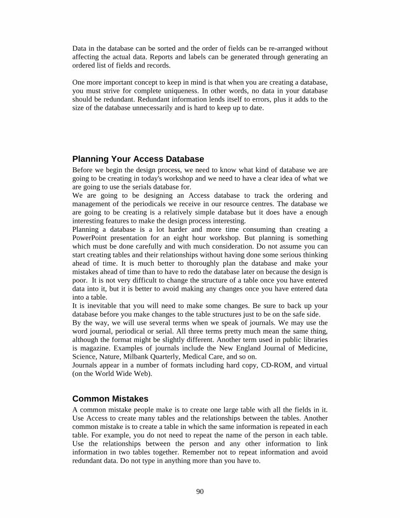
90

Data in the database can be sorted and the order of fields can be re-arranged without affecting the actual data. Reports and labels can be generated through generating an ordered list of fields and records. One more important concept to keep in mind is that when you are creating a database, you must strive for complete uniqueness. In other words, no data in your database should be redundant. Redundant information lends itself to errors, plus it adds to the size of the database unnecessarily and is hard to keep up to date.

Planning Your Access Database Before we begin the design process, we need to know what kind of database we are going to be creating in today's workshop and we need to have a clear idea of what we are going to use the serials database for. We are going to be designing an Access database to track the ordering and management of the periodicals we receive in our resource centres. The database we are going to be creating is a relatively simple database but it does have a enough interesting features to make the design process interesting. Planning a database is a lot harder and more time consuming than creating a PowerPoint presentation for an eight hour workshop. But planning is something which must be done carefully and with much consideration. Do not assume you can start creating tables and their relationships without having done some serious thinking ahead of time. It is much better to thoroughly plan the database and make your mistakes ahead of time than to have to redo the database later on because the design is poor. It is not very difficult to change the structure of a table once you have entered data into it, but it is better to avoid making any changes once you have entered data into a table. It is inevitable that you will need to make some changes. Be sure to back up your database before you make changes to the table structures just to be on the safe side. By the way, we will use several terms when we speak of journals. We may use the word journal, periodical or serial. All three terms pretty much mean the same thing, although the format might be slightly different. Another term used in public libraries is magazine. Examples of journals include the New England Journal of Medicine, Science, Nature, Milbank Quarterly, Medical Care, and so on. Journals appear in a number of formats including hard copy, CD-ROM, and virtual (on the World Wide Web).

Common Mistakes A common mistake people make is to create one large table with all the fields in it. Use Access to create many tables and the relationships between the tables. Another common mistake is to create a table in which the same information is repeated in each table. For example, you do not need to repeat the name of the person in each table. Use the relationships between the person and any other information to link information in two tables together. Remember not to repeat information and avoid redundant data. Do not type in anything more than you have to.

91

General Questions to Ask Yourself Before You Begin There are a number of questions you need to ask yourself before you start. Why do I think I want a database? Does the information I have lend itself to fields and records? (Most information lends itself to some kind of structure). What kind of data do I have? What is the best way to organize it? (These questions help you define your tables). If I need to enter data into a table, how can I simplify the process to make it as easy as possible for someone to do data entry? (This question helps you define the forms you may need). When I have the data entered into the database, what kinds of questions do I think I’ll want to ask about it later on? (This question will help you define the queries and reports you will want to make based on your data).

Collecting Information on the Database Be sure to identify and talk to potential users, even if you spend your days working in the area of the database you're going to create. You would be surprised as how often you forget important elements. Be certain to record the suggestions. Professionals who create databases for a living generally use Requirement Collection Forms to capture requests for data elements from the people they interview.

The Design Process • Determine the purpose of our database • Determine the tables we need for the database • Determine which fields we will need • Determine how each of the tables is related • Refine and redefine the design

Determine the Purpose of our Database Before we do anything else, we need to ask the following questions: What do we need to know from our database and what will this information allow us to do?

What do we need to know from our database? We'll need to know a lot. This database is going to track a lot of information and should be able to answer any serials-related questions we have.

Relationships Once you have built tables, you need some method of bring the information in the tables back together. You need a relationship between the tables and those relationships need to be defined. Once you get the relationships built, you can create queries, and forms and reports from several tables at once. Building relationships is frustrating even if you understand the theory of building entity relationship diagrams. (We will not be covering the theory for this material). For those who have not been trained in computer science, it can sometimes be a nightmare. As mentioned elsewhere, I spend a good deal of my time gnashing my

92

teeth, muttering under my breath, and even crying tears of frustration as I try to figure out what the relationships are. (They are as difficult as human relations and about as complex). Microsoft Help says that a "relationship works by matching data in key fields, usually a field with the same name in both tables. In most cases, these matching fields are the primary key from one table, which provides a unique identifier for each record, and a foreign key in the other table".

Types of Relationships You can create several types of relationships between tables: • one to many • one to one • many to many

One to Many Relationship A one-to-many relationship is the most common type of relationship. In a one-to-many relationship, a record in Table A can have many matching records in Table B, but a record in Table B has only one matching record in Table A. For example, one publisher can publish many journals, but it's highly unlikely that a journal would have more than one publisher. Simularly, one bindery could receive many volumes each year to be bound, but each volume would only go to one bindery.

One to One Relationship In a one-to-one relationship, each record in one table can have only one matching record in a second table, and each record in the second table can have only one matching record in the first table. This type of relationship is fairly uncommon, because most information related in this way would be in one table. We do not have any examples of a one to one relationship in our serials database.

Many to Many Relationship In a many-to-many relationship, a record in one table (table 1) can have many matching records in a second table (table 2), and a record in table 2 can have many matching records in table 1. This type of relationship is only possible by defining a third table (called a junction table) whose primary key consists of two fields - the foreign keys from both Tables 1 and 2. A many-to-many relationship is really two one-to-many relationships with a third table. We have one example of a many to many relationship in our serials database.

93

Using the Menu bar

• The Menu bar contains all of the Access menu options. With these menu options, you can access most of the Access features. The options available in each menu often depend on the object you are working with and the mode of Access .

• By default, the Menu bar appears at the very top of the screen. However, you can place this bar wherever you want on the screen.

• To move the Menu bar, find the small gray lines at the far left of the menu bar. Place your mouse on these lines. The mouse indicator changes to a four-arrow symbol. This means you can drag the bar to your desired location:

Using the Database toolbar

• The Database toolbar is a bar of buttons that act as shortcuts to many of the Access features that are most often used. This toolbar is very similar to other applications' Standard toolbar.

• By default, the Database toolbar appears at the top of the screen, just below the Menu bar. Like the Menu bar, though, you can place this bar wherever you want it on the screen.

• To move the Database toolbar, find the small gray lines at the far left of the Database toolbar. Place your mouse on these lines; the mouse indicator changes to a four-arrow symbol. This means you can drag the bar to your desired location:

Using the Task Pane

• The Task pane is a window that acts like a dialog box, except you can keep it on the screen as you work. Depending on the task it relates to, it provides access to different features.

• Access provides three Task panes: New File, Clipboard , and Search. You can change the type of task pane by clicking the down arrow in the top right corner of the Task pane, the three types are then available on a drop-down menu.

• One example of a Task pane is when you create a new database file (by choosing File > New). The various options for creating a new database file are then provided in the pane.

ACCESS WORKSPACE

94

• As with toolbars, you can move the Task pane around the screen. Do this by dragging its title bar.

• If the Task pane is too small for you, you can resize it. Do this by positioning the mouse indicator over a side edge or corner of the Task pane. The mouse indicator changes to a two-sided arrow, which means you can drag it to make the pane bigger or smaller:

Using the Status bar

• The Status bar appears at the bottom of the screen. It provides status information. For example, if you are inputting information into a table, the status bar might tell you what mode you are in or what column you are currently applying changes to.

• The following image shows the Status bar when you have the Database window open:

• The following image shows the Status bar when you have a Design view open:

• Unlike the other toolbars, you cannot move the Status bar around the screen.

Using the Office Assistant

To open the Office Assistant:

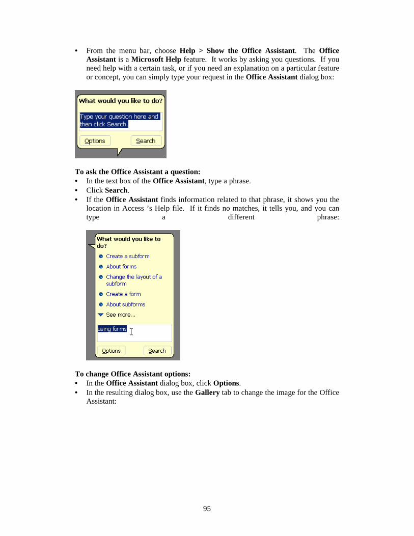
95

• From the menu bar, choose Help > Show the Office Assistant. The Office Assistant is a Microsoft Help feature. It works by asking you questions. If you need help with a certain task, or if you need an explanation on a particular feature or concept, you can simply type your request in the Office Assistant dialog box:

To ask the Office Assistant a question: • In the text box of the Office Assistant, type a phrase. • Click Search. • If the Office Assistant finds information related to that phrase, it shows you the

location in Access ’s Help file. If it finds no matches, it tells you, and you can type a different phrase:

To change Office Assistant options: • In the Office Assistant dialog box, click Options. • In the resulting dialog box, use the Gallery tab to change the image for the Office

Assistant:

96

• Use the Options tab to configure the behavior settings for the Office Assistant:

• Click OK to apply the changes and close the dialog box. To hide the Office Assistant: • From the Help menu, choose Hide the Office Assistant. You can also right-click

the Office Assistant image and choose Hide on the context menu.

Customizing the toolbars

• You can right-click any toolbar and choose Customize on the context menu to customize the appearance and behavior of Access ’s toolbars:

97

• In the Customize dialog box, use the three tabs to specify what toolbars should

appear and how you want the commands to work:

• When the Customize dialog box is showing, you can right-click any button or

menu option to customize names, button images, properties, and so on:

98

99

Creating Database Files A database file is the actual information repository - it is a collection of related data that has to do with a particular subject. For example, if you owned a retail chain, you might want to place all sales and store information in a database. You could organize this data into tables; you could group employee information in one table, customer information in another, and store information in yet another. • Microsoft Access lets you create two main types of files: database files (with an

.mdb extension) and project files (with an .adp extension). • A project file is a file that connects to the database - it is the basis for

client/server applications. For example, a project file might contain forms, reports, or modules; it would not contain any data or data-definition-based objects (like tables). Think of a project as an “in-between” file: it serves as the interface for an actual database file. Creating a new database file

• From the menu bar, choose File > New OR press the Ctrl + N key combination to open the New File task pane which appears on the right of your screen:

• Click Blank Database. In the File New Database dialog box, specify a location

and a name for your new database file. Then click Create:

100

• The Database dialog box appears to let you start adding objects and information

to your database. We’ll deal with these features in a future section of this course:

Opening and Closing a Database File

Opening a database file

• From the menu bar, choose File > Open OR press the Ctrl + O key combination to display the Open dialog box. Browse to the location of the database file you want to open. When you find it, highlight it and click Open:

101

Note: You can also double-click the file to open it.

Closing a database file

• From the menu bar, choose File > Close.

Using the Open a File Area of the New File Task Pane

Opening the New File task pane

• From the menu bar, choose File > New. • The New File task pane opens as a window on the right side of the screen.

Viewing and opening recent files

• The Open a File area of the New File task pane shows recently opened Access files:

• If the list does not include the file that you want to open, click More Files. • The Open dialog box opens, which lets you browse to the location of a file,

specify its name and type, and open it:

102

• To open a file in the list, simply double-click its name.

Using the New Area of the New File Task Pane

Using the Blank Database option

• The Blank Database option lets you create a new database file from scratch. You’ll then be able to add new tables and other database objects, also from scratch:

• To use this option, click Blank Database. The File New Database dialog box

opens. • In the File Name box, type a name for the new database, and from the Save As

Type list, choose a file format (usually .mdb for a Microsoft Access database). • Use the Save In list to browse to the location in which you want to place the new

database file. You can double-click folders in the large pane to open them. • Click Create when you have entered all the required information.

103

Data Access Page option

• The Blank Data Access Page option lets you create a new data access page from scratch. A data access page is a Web page that is connected directly to the data in your database. You can use a data access page to view, edit, update, delete, filter, group, and sort information in the database:

• A data access page can contain components such as a spreadsheet, a PivotTable

list, or a chart. • Data access pages only work in Microsoft Internet Explorer 5 or later. • To use this option, click Blank Data Access Page. A view of the blank page

appears:

• Create the page as desired. Use the toolbox that appears along with the view to add text and other objects to the page.

Note: If the toolbox doesn’t appear, you can view it by choosing View > Toolbox. To make a page available to other users over the World Wide Web: • You need to save the page to a Web folder or Web server. • You also need to make the database (the one connected to the data access page)

available to the users.

104

Using the Project (Existing Data) option

• The Project (Existing Data) option lets you create a new project file based on an existing database file. A project file is a file that connects to the database; it is the basis for client/server applications. For example, a project file might contain forms, reports, or modules; it would not contain any data or data-definition-based objects (like tables):

• When you choose this option, the File New Database dialog box opens. This dialog box lets you specify a name and location for the new project file.

• When you click Create in the File New Database dialog box, the Data Link Properties dialog box opens. This dialog box lets you provide the necessary information for Access to connect the new project file with an existing database:

Using the Project (New Data) option

• The Project (New Data) option lets you create a new project file that is not yet based on any database file:

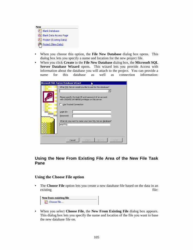
105

• When you choose this option, the File New Database dialog box opens. This

dialog box lets you specify a name and location for the new project file. • When you click Create in the File New Database dialog box, the Microsoft SQL

Server Database Wizard opens. This wizard lets you provide Access with information about the database you will attach to the project. You can provide a name for this database as well as connection information:

Using the New From Existing File Area of the New File Task Pane

Using the Choose File option

• The Choose File option lets you create a new database file based on the data in an existing file:

• When you select Choose File, the New From Existing File dialog box appears. This dialog box lets you specify the name and location of the file you want to base the new database file on.

106

• You can base a new database file on any of the following file types: another Access database file (*.mdb), an Access project file (*.adp), or an HTML file (*.htm or *.html ).

Using the New From Template Area of the New File Task Pane

Using the General Templates option

• The General Templates option lets you create a new file (either a database file or a project file) based on one of Access’s predefined templates:

• When you choose General Templates, the Templates dialog box opens with two

tabs: the General tab and the Databases tab. • Use the General tab to create a new blank database, blank data access page,

project (based on an existing file), or project (not based on an existing file). These are the same options as the ones listed in the New area of the New File task pane:

• Use the Databases tab to view a list of predefined Access databases. To model

your new database file on one of these, select it and click OK :

107

• The right half of the Templates dialog box (for both options) lets you change the

manner in which the files are listed in the left half. For example, if you want to view the contents of the left half in list format instead of icon format, you can select the appropriate button on the right half.

Using the Templates On Microsoft.com option

• The Templates on Microsoft.com option lets you create a new file based on a Microsoft predefined template located on Microsoft web site:

• This option is a link that launches your Internet browser and brings you to a

Microsoft Office web page. Follow the instructions on this page to view the available templates.

The Database Menu Bar

Using the Database Menu Bar

• The Database Window Menu bar allows you to open an object, access Design view for the selected object, create a new object, delete an object, and arrange the objects in the Database window.

Using the Open button

108

• The Open button of the Database window menu bar allows you to view an object in your database:

• The Open button works in conjunction with the object you have currently selected in the window. For example, if you have a particular table selected and click the Open button, a window containing that table opens.

Using the Design button

• The Design button allows you to view an object in Design view. Design view is a mode of Access that lets you create or modify the structure of tables and queries, create forms or pages through which you can display data, and format reports:

• Like the Open button, the Design button works in conjunction with the object you

have currently selected in the window. • The options within the Design view depend on the object you are modifying. For

example, Design view for tables differs from that for forms.

Using the New button

• The New button allows you to create a new object using a wizard:

• The New button works in conjunction with the type of object button selected in

the toolbar along the left side of the Database window. For example, to create a new table, select the Tables button and click New.

109

Using the Delete button

• The Delete button allows you to delete an object:

• To use this feature, select the object you want to delete and click this button. As a

safeguard, Access will always prompt you to continue before it actually deletes the object.

Using the Icon buttons

• The Large Icons and Small Icons buttons allow you to change the size of the graphics in the Database window.

• Click Large Icons to make the graphics bigger:

• Click Small Icons to make the graphics smaller:

Using the List button

• The List button allows you to view the database objects in the Database window in a list format:

110

• In this list, only the names of the objects are listed.

Using the Details button

• The Details button is similar to the List button (it also lets you view the database objects in list format), but it provides additional information to just the name, such as a description of the object, the date it was last modified, and its type:

• To add a description to an object (so it appears under the Description column

when you click the Details button), right-click an object in the Database window and choose Properties. In the Properties dialog box, you can type the description in the box provided. After you close this dialog box, the description will appear when you have the list details showing:

Create a Table

111

About creating a table in Design view

• You can create a table in Design view or with a wizard. • Design view is a window that lets you configure the table columns (also called

fields). Think of this view as a blueprint for the table: it doesn’t show you actual data in each row, but it does define how the rows need to look:

• The concept of “row” has a slightly different meaning in Design view: a “row” in

Design view actually represents one column in the table (as opposed to one record). For example, if in Design view you name a row “First Name”, the table will have a column called “First Name” and each record in the database will need to have a “First Name” field entry.

• All fields have two main characteristics: Field Name and Data Type. Field Name refers to the name of the column. Data Type refers to the type of information a field can contain (e.g., text instead of numbers).

• For each field, you can also define other properties, such as how many characters they can hold, or how they should be presented to users (e.g., as a drop-down list instead of a text box).

• It’s usually a good idea to define one field in the table as a primary key . A

primary key is a field whose value uniquely identifies each record in the table. Access provides an AutoNumber feature that can assign a unique number to each record for this purpose. For example, if you are creating an Employees table, you can create an Employee ID field, define it as the primary key, and use the AutoNumber feature to give each employee record a unique ID. Primary keys are used as the basis for relationships to foreign keys of other tables. A primary key cannot allow Null values:

112

• You can use the Tab key to move from field to field.

Creating a Table in Design View

• Click the Tables button along the left side of the Database window. • In the right pane, double-click Create table in Design view. A blank design view

window opens. • Begin creating fields: input a name and type for each. When you place the cursor

in the Data Type field, a drop-down arrow lets you choose a type:

• For each field, use the tabs at the bottom of the window to further define field

properties. If you need more information about these properties, place your cursor in each; the lower right corner of the window tells you how that property works:

• Use the Insert Rows or Delete Rows buttons on the toolbar at the top of the

Access window to add new rows above your current row or delete your current row:

113

• Use the Primary Key button on the toolbar at the top of the Access window to make the current row the primary key. If you want to remove primary key status from that row, select it and click the Primary Key button again.

Note: You can also right-click a row and choose Primary Key from the context menu:

• When you are finished creating fields and setting up the table as desired, choose

File > Save and type a name for your table.

About using the Table Wizard to create a table

• The other method for creating a table is by using a wizard. This wizard provides samples of common fields in different types of personal or business database tables. Note that there is no actual data attached to these fields; they are merely models that you can choose to incorporate. You can always rename the fields if you want a different name.

Using the Table Wizard to create a table

• Click the Tables button along the left side of the Database window. • In the right pane, double-click Create table by using wizard. The wizard opens. • On the first page, use the Business or Personal options to filter the list of sample

tables and fields to the desired type. Clicking different tables in the Sample Tables list makes the contents of the Sample Fields list change accordingly. When you see a field name that matches a field you want in your new table, select it and click the > arrow button:

• Fields you have added stay in the list on the right even if you change the options in the left half of the dialog box. If you want to remove a field from the list select

114

it from the list on the right, and click the < arrow button. If you would like to rename a field, select it and click Rename Field.

• Click Next. Type a name for your table and choose whether you want the wizard

to set a primary key. If you choose No, you’ll need to do it in Design view after the table is created. If you choose Yes, you can always change the primary key after the table is created:

• Click Next. If you chose to let the wizard set a primary key for you on the

previous page, you can now create relationships between this table and other existing tables if there is common information between the tables. The wizard lists all other existing tables; if you select one and click Relationships, the wizard asks you the type of relationship (and gives an explanation of each):

• If you chose to set your own primary key on the previous page, the wizard asks you for information that might be suitable for a primary key:

115

• Click Next. If you chose to manually set your primary key, you are now

prompted to specify relationships (described above). Otherwise, the final wizard screen appears.

• Choose an option for when the wizard finishes: you can have the wizard open Design view for you to modify the table design, start entering data directly into the table OR have the wizard open a form for data entry:

• Click Finish.

116

Forms can be used for data entry, displaying data in a user-friendly format, and as a navigational tool.

Using Forms

• A form is a type of interface you can create between you (or any user) and the database. Forms can be as simple or complicated as you want.

• The simplest type of form is a data-entry form. This type of form simply displays data from the database. For example, if you had a query that returned a set of values, you could display these values in a form.

• Another type of form is a switchboard form. This type of form can have links to (and open) other forms, and it can open reports.

• The third type of form is a custom dialog box. This type of form can accept user input and execute an action based on the input.

• A bound form is a form that is bound to one or more tables in the database. The data is stored in the underlying table (called the record source) and referenced into the form; the form’s organizational information (like title, date, and page number) is stored in the form’s design.

• You can change the form’s appearance by adding graphics, lines, text, or other types of appearance-oriented features. For example, if you need to include a company logo on form to apply a uniform and standard look to your database, you can easily do so.

• The easiest way to create a form is to use the wizard that Access provides. This wizard lets you choose the fields or records from a table or a query that you have saved. Once the wizard places the appropriate data in the form, you can use Design view to customize the form’s appearance. If you want, you can also create a form from scratch in Design view.

• When the form is finished and you open it, it appears in its own window. You can click the arrow buttons in the bottom left of this window to move through various records.

Creating and Using Data Entry Forms

117

• Forms can have different sections to them. Usually, the data (presented in text boxes or other user interface objects) appear in the Details section. You can also add a Header or Footer section to the form, perhaps to contain page numbers.

Creating forms with the wizard:

• In the Database window, click the Forms button on the toolbar along the left side of the window:

• Double-click Create form by using wizard. The Form Wizard opens:

• On the first page of the form, specify where you want the data for the form to come from. The Tables/Queries drop-down list shows all table and queries you have created; when you select one of these, the fields from that table or query appear in the Available Fields list.

• Double-click fields in the Available Fields list to move them to the Selected Fields list.

118

Note: You can also select a field and use the arrow buttons to move them back and forth between the lists.

• When the Selected Fields list contains all the fields you want to be part of the form, click Next.

• On the next page of the wizard, choose one of the layout options. When you select the option, Access shows you a preview of that presentation option in the left side of the dialog box. When you are done, click Next:

• On the next page, choose one of the built-in styles to give your form attractive and

professional look. Choose one of the styles listed. When you select an option, Access shows you a preview of that style in the left side of the dialog box. When you are done, click Next:

119

• On the last page of the wizard, specify a name for the form. After you are finished with the wizard, this name will appear in the Database window when you select the Forms button:

• Tell the wizard what to do when it closes. You can display the form immediately, or you can view the form’s design in Design view.

• Click Finish.

Move between records or fields

Move between records by using navigation buttons in a form The navigation buttons are located at the bottom of the window in Datasheet or Form view. You can use these buttons to move quickly between records.

1 First record 2 Previous record 3 Record number 4 Next record 5 Last record 6 New record

120

Modifying a form in Design view

• If the form you want to modify is not already in Design view, do the following: in the Database window, with the Forms button selected, select the form and click the Design button on the Database window’s toolbar. (You can also right-click the form and choose Design View from the context menu.) The form opens in Design view:

• By default, a toolbox with various formatting options should appear alongside the

form. If this does not happen, you can turn the visibility of the toolbox on or off by clicking the Toolbox button on the toolbar at the top of the screen. You can resize the toolbox if you want by dragging the corners or edges of the toolbox to the new dimensions.

• Use the options in the toolbox to add elements of design to the form. When you hold the mouse over each option, a ToolTip message tells you what that option does:

• After you select a toolbox item, move the mouse indicator over top of the form. You’ll notice that the mouse indicator changes to show the tool that you have selected. Drag a box on the form to create the object.

• For example, if you want to add a label to the form, click the Label button in the toolbox. Move the mouse indicator over top of the form to the location where you want to type the label. Drag a box in the approximate shape of the label. As soon as you release the mouse button, a box will appear, with the cursor blinking in this box: this means you can start typing text for the label in the box. As soon as you are done, press the Enter key, and the label is complete:

121

To resize an object in Design view: • If you need to resize an object that you have added to the form, click the object.

Access shows little black squares along the sides of the object. These black boxes are resize handles: click and drag one to resize the object. When you are done, click away from the object; the black boxes disappear, and the object appears with the new size you have configured:

Creating Page Headers and Footers

• Page headers and page footers appear at the top and bottom of each page and can display information such as a column heading.

To create page headers and footers: • Right-click in the Detail area of the form. • From the pop-up menu, select Page Header/Footer. This opens the Page Header

and Page Footer panes:

• Place the desired control on the page header or page footer. • From the pop-up menu, select Form Header/Footer. This opens the Form

Header and Form Footer panes.

122

• Place the desired control on the form header or form footer. Note: Page headers and footers and Form headers and footers can both appear on the same form.

To add headers and footers to a form in Design view: • You can add headers and footers to a form in Design view, similar to headers and

footers in a Microsoft Word document. For example, you could place a page number in the header or footer, or insert a company logo.

• To create a header and/or footer, right-click anywhere in the form and choose Form Header/Footer from the context menu. You will notice that Access creates a Form Header section at the top of the form and a Form Footer section at the bottom of the form. Each of the section headings displays as a bar across the width of the form, and each of these bars has a small gray box at its left-most edge:

• To resize the sections, hold the mouse on the section bar’s top or bottom edge.

The mouse indicator changes to show arrows on the top and bottom. Drag up or down to make the section bar appear higher or lower. For precise positioning, use the ruler that’s provided along the left edge of the form window.

• You can add objects from the toolbox to a header section or a footer section in the same way as you would for the Detail section.

• You can edit properties for any of the sections by right-clicking the section bar and choosing Properties from the context menu.

To insert page numbers in a header or footer: • From the menu bar, choose Insert > Page Numbers. • In the top part of the Page Numbers dialog box, choose whether you want the

page number to appear on its own (e.g., Page 1) or along with the total number of pages in the form (e.g., Page 1 of 8):

123

• In the middle part of the dialog box, choose whether you want the page number to

appear in the header section or the footer section. • In the bottom part of the dialog box, specify how you want the numbers to be

aligned on the form and click OK .

Inserting an image that does not change from record to record

To insert an unbound image (which will be the same for all records): • Open the form in Design view. • Make sure that the toolbox is showing. If not, click the Toolbox button on the

toolbar. • Click the Image button in the toolbox:

• In the form itself, click where you want the image to appear. The Insert Picture

dialog box then opens. • Find and select the image that you want to insert. Then click OK to insert it. • Right-click the image and choose Properties from the context menu. • On the Format page of the Properties dialog box, click in the Picture cell and

use the drop-down list to specify whether the picture should be linked or embedded.

124

• Use the other picture-related settings in the Properties dialog box (described in the previous procedure) to size and place the image appropriately. Then close the Properties dialog box.

• To move or resize the image manually, click the image. When you hold the mouse indicator over the image, the indicator turns into the image of a hand. You can then drag the image to a new location. If you select and drag one of the small black boxes along the edges of the image, you can resize it.

Replacing an image

To replace an unbound background image: • Open the form in Design view. • Right-click the form’s title bar and choose Properties from the context menu. • On the Format page, click in the Picture cell. • Click the Browse button beside this cell. • Browse to a different image and click OK .

Choosing an Appropriate Control

• Controls are objects that can be placed on forms, reports, or data access pages that display data, perform actions, or can be used for visual display. Controls shipped with ACCESS include:

• Text Boxes: Used to display data on a form. Text boxes can be bound to a data source or unbound to accept input or display a calculation.

• Labels: Used to display text on a form. Labels are useful for descriptive of instructional text. Labels are not associated with a data source.

• List Boxes: Used to display a pre-determined list of values. List boxes are useful when limiting selection choices or when enforcing data integrity.

• Command Buttons: Used to execute a pre-defined set of actions in a macro or event procedure written in visual basic.

• Check Boxes: Used to set Yes/No values from an underlying query or table. • Option Groups: Used to select a limited list of choices. Sometimes

interchangeable with List Boxes when selecting from only a few pre-defined options.

• Toggle Buttons: Used to set Yes/No values from an underlying query or table. Useful when combined with an Option Group to select values that are Yes/No.

• Image: Used when displaying a digital image on a form. An example would be the display of a company logo.

• Tabbed Pages: Used when presenting different sections of information as one logical set. Useful when separating levels of information related to a common topic such as employee, company, or personal information.

• Rectangles and Lines: Used when displaying limited geometric shapes. Useful when displaying breaks between fields or sections within a form.

• Subform: An advanced control that displays child data that is related to data on the parent form. Subforms are discussed later in this training manual.

125

Creating Queries

About queries

• A query is similar to the idea of filters discussed earlier: it is a way to search for data in your database. Unlike filters, though, which can only work within a single datasheet (or table) at a time, queries can let you search multiple tables at once.

• Access lets you create five main types of queries: Select queries, Parameter queries, Crosstab queries, Action queries, and SQL queries.

• A Select query is the most common type of query. You can use it to find and return data from one or several tables, displaying the found data in a datasheet. When creating a Select query, you can instruct Access how to group the records it retrieves and calculate sums, counts, averages, or other types of operations on the retrieved data.

• Think of a query as a set of instructions from you (the user) to the database: “Database, give me all records from the Employees table where the Last Name field of the record equals “Jones” and the Phone Number field contains the numbers ‘123’.” It’s possible that only one employee named Jones will be returned, or maybe the query will find no matching data: either there are no “Jones” employees in the table, or the “Jones” employees that were found do not have a ‘123’ in their phone number.

• You can make the query as precise as you want, to return only very specific information, or you can make the query broad, to return multiple records.

• When creating the query, you can also tell Access how many fields of the records you want returned. For example, if you want to retrieve all employees with the last name “Jones”, and you only want to see the First Name and Last Name fields of the records matching that criteria, you can specify only those two fields in the query. This lets you focus your results set on only meaningful data, so that the datasheet does not get too confusing.

• The data that Access finds in response to your query is called the results. Some other database applications call this returned data a results set.

• You can save queries to reuse them. This is a helpful feature if the data in the database continually changes, but you often search for the same type of information. For example, if you regularly need to search for sales in excess of $10,000 for any product, you can build and save a query to search the Sales fields when for values exceeding $10,000. You can then reuse this query each week or month; your search criteria doesn’t change even though the data does.

• When working with queries, you should be aware of some presentation conventions. First, table columns (or fields) are sometimes presented as tablename.fieldname. For example, the Last Name field in the Employees table might be shown textually as Employees.Last Name. This can help to avoid confusion if two tables have the same field name. Second, an asterisk (*) can represent all fields in a table. For example, Employees.* would mean all fields in the Employees table.

126

About creating a new query in Design view

• Access lets you create queries in one of two ways: in Design view or by using a wizard.

• For the Design view method, Access operates in a similar way to the Design view of creating a table: you build the structure of the query by working with the list of fields that Access provides.

• When you create a query in Design view, you can have the query span multiple tables. To do so, however, you need to create relationships between tables. The concept of relationships is a more advanced feature of Access, and it is not described in detail in this Foundation level. This level concentrates on teaching you to run a query on one table at a time.

• Design view lets you drag-and-drop items from a table into the grid in the lower pane.

Requirements for a query in Design view

• A simple query in Design view consists of the following elements: • First , you need to specify the field(s) you want involved in the query. • Second, you need to specify the table each field belongs to. • Third , you can optionally tell Access to sort the results based on a field. For

example, if you have selected the Last Name and First Name fields and you want the results sorted alphabetically by Last Name, you can do an Ascending sort on the Last Name field.

• Fourth , you need to specify which fields you want to appear in the results. This is not the same thing as the second requirement. For example, you can build the query so that it looks for information in two different fields, but only shows one field in the results.

• Fifth , you need to give the actual criteria for the query. In other words, you need to tell Access what information you want it to search for.

Creating a new query in Design view

• In the Database window, click the Queries button on the toolbar along the left side of the window:

127

• Double-click Create query in Design view. A query window opens. If you have multiple tables in your database, the Show Table dialog box also opens:

• If the Show Table dialog box opens, on the Tables tab, select the table(s) that you

want to query and click Add. A box listing that table’s columns (or attributes) then appears in the pane at the top of the query window.

• Close the Show Table dialog box when you are finished with it. • Choose the fields you want involved in the query. You can do this in one of two

ways: • First , you can double-click a field listed in the table box in the top pane; the field

then appears in the first empty column in the bottom pane:

• Second, you can place the cursor in a box in the Field row; a drop-down arrow

appears, letting you select a field. If you use the second method, be aware of the following: if you have multiple tables open in the top pane, and if no information appears in the Tables row immediately below where you click, the drop-down list will contain all fields from all visible tables, in the form of tablename.fieldname.

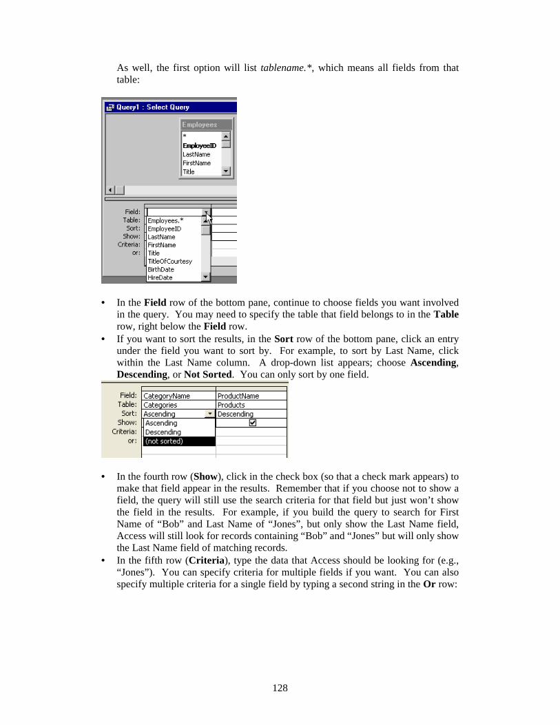
128

As well, the first option will list tablename.*, which means all fields from that table:

• In the Field row of the bottom pane, continue to choose fields you want involved

in the query. You may need to specify the table that field belongs to in the Table row, right below the Field row.

• If you want to sort the results, in the Sort row of the bottom pane, click an entry under the field you want to sort by. For example, to sort by Last Name, click within the Last Name column. A drop-down list appears; choose Ascending, Descending, or Not Sorted. You can only sort by one field.

• In the fourth row (Show), click in the check box (so that a check mark appears) to

make that field appear in the results. Remember that if you choose not to show a field, the query will still use the search criteria for that field but just won’t show the field in the results. For example, if you build the query to search for First Name of “Bob” and Last Name of “Jones”, but only show the Last Name field, Access will still look for records containing “Bob” and “Jones” but will only show the Last Name field of matching records.

• In the fifth row (Criteria ), type the data that Access should be looking for (e.g., “Jones”). You can specify criteria for multiple fields if you want. You can also specify multiple criteria for a single field by typing a second string in the Or row:

129

• If you want the criteria to involve a mathematical operator (e.g., sales greater than

$10,000), place the cursor in a Criteria field and click the Build button on the toolbar:

• The Expression Builder dialog box opens. In this dialog box, use the pane at the top to build the expression. You can add operators by clicking the buttons below this pane.

• You can have Access show you common expressions by clicking the folders in the bottom left corner of the dialog box and then double-clicking the entries that appear in the right panes to add them to the top pane:

• When you have built the query to the appropriate specifications, click the Run

button on the toolbar. Access returns all matching records in a new window:

130

• To re-show the Design window, click the View button in the top left corner of the toolbar:

About creating a new query using a wizard

• The other method for creating a new query is by using a wizard. This wizard takes you through the various steps of building a simple query.

• The requirements for a building a query in this way are similar to those for building a query in Design view; you need to provide the same basic units of information.

• The screens of the wizard may vary, depending on the selections you make on an earlier screen. That’s why the procedures below are broken up according to option selections.

• If you need to revise your design, you can always click the Back button in the wizard to return to an earlier step.

Creating a numerical query using the wizard

To create a query that includes a numerical field: • In the Database window, click the Queries button on the toolbar along the left

side of the window. • Double-click Create query by using wizard. The Simple Query Wizard opens:

• On the first page, select the fields you want involved in the query. From the Tables/Queries drop-down list, choose a table. The available fields from that table then appear in the Available Fields list.

131

• Double-click a field to add it to the Selected Fields list OR select one of the Available Fields and click the arrow > button.

• You can remove a field from the Selected Fields list in the same way. Double-click one of the fields from the Selected Fields list OR select one of the fields and click the ‘Back’ arrow < button.

• Make sure you include a numerical field. • When you are finished, click Next. On the next page, tell the wizard how you

want the information returned:

• Choose the Detail option if you want every field (of records that match the search

criteria) returned. Choose the Summary option if you want Access to summarize the numerical data. You can specify the summary action by clicking Summary Options and providing the desired information in the resulting dialog box. If you want Access to show you a count of all the records it finds, select that check box and click OK to close the dialog box.

132

• Click Next to type a name for the query:

• To run the query and have the results returned to you, select Open the query to

view information and click Finish. • To hold off on running the query and to view the structure of the query in Design

view before running it, select Modify the query design and click Finish. A query window containing the parameters you have specified opens; you can modify the query as desired. Click the Run button on the toolbar to run the query and see the results:

Creating a non-numerical query using the wizard

To create a query that does not include a numerical field: • In the Database window, click the Queries button on the toolbar along the left

side of the window. • Double-click Create query by using wizard. The Simple Query Wizard opens:

133

• On the first page, select the fields you want involved in the query. From the Tables/Queries drop-down list, choose a table. The available fields from that table then appear in the Available Fields list.

• Double-click a field to add it to the Selected Fields list (or select one and click the arrow > button).

• You can remove a field from the Selected Fields list in the same way: double-click it or select it and click the ‘Back’ arrow < button.

• Do not include a numerical field. When you are finished, click Next. • On the next page, type a name for the query:

• To run the query and have the results returned to you, select Open the query to view information and click Finish.

• To hold off on running the query and to view the structure of the query in Design

view before running it, select Modify the query design and click Finish.

134

• A query window containing the parameters you have specified opens. Here you can modify the query as desired.

• Click the Run button on the toolbar to run the query and see the results:

Saving queries

• You can save a query in multiple ways. • If you are working in the Database window, you can click the Queries button on

the left. Then right-click an existing query and choose Save As from the context menu. Type a new name to save the query with a different name. You can choose to save it as a query, form, report, or data access page.

• If you have the Results window open, from the menu bar, choose File > Save As. Type a name for the query. You have the same save options as in the step above:

• If you have the Query Design view open, from the menu bar, choose File > Save As. Type a name for the query. You have the same save options as in the step above.

Opening an existing query’s result window

• Access shows all existing queries in the Queries view of the Database window. • To open a query, click the Queries button on the toolbar on the left side of the

Database window:

135

• Double-click a query. • The results of that query appear in a window

Open an existing query in Design view

• Click the Queries button on the toolbar on the left side of the Database window. • Select a query. • Click the Design button at the top of the Database window.

Note: You can also right-click a query and choose Design View from the context menu:

Refining the results of a query

• After you run a query, its results are displayed in a separate window. Take a moment to scan through the results; you may find that the information was not what you expected, or the wrong information appears. Often, an incorrect query is the result of errors in the criteria that you give Access when constructing the query:

• You can revise a query’s construction in Design view. To refine results, take a

look at all of the parameters you have specified in Design view. Ask yourself whether the fields, tables, and search criteria you have specified are related to the desired information.

• After you make some changes, you can re-run the query simply by clicking the Run button on the toolbar. If that result set is not sufficient, you can continue to modify the query in Design view and re-run the query until you get the results you want:

136

Creating and Using Reports A report is a way to present information in a format that’s suitable for printing. You can rearrange the information and configure the presentation so that it best suits your purposes. • Reports are an effective tool for analyzing information. You can create a report

that summarize data from the database, and then print the report to analyze numbers and trends.

• Reports are generally bound to one or several tables (or queries) in the database. The data that appears in the report is linked in from the fields in the underlying table or query. Other information on the report, like labels or titles or page numbers, are saved with the report itself (not with any underlying data source.)

• A report does not need to contain fields from each of the tables or queries it’s based on.

• You can create links between a report and its underlying data source (e.g., tables or queries) by using graphical objects called controls. An example of a control is a text box: it displays data from a field in the underlying table.

• You can customize the report’s design to make it more attractive. • There are three ways to create a report.

o First , you can create a report based on one table or query using a feature called AutoReport. AutoReport then creates a report that displays all the fields and records in the underlying table or query.

o Second, you can create a report using a wizard. This wizard guides you through the process of selecting tables (or queries) and fields to serve as the basis for the report.

o Third , you can create a report from scratch in Design view (similar to creating tables, queries, and forms in this way.)

Creating a report using AutoReport

• In the Database window, click the Reports button along the left side of the window:

137

• On the toolbar at the top of the Database window, click the New button. The New Report dialog box opens:

• In the New Report dialog box, select an AutoReport option. Choose

AutoReport: Columnar to create a report in which each field appears on its own line with a label to its left. Choose AutoReport: Tabular to create a report in which the fields of each record appear on the same line, and the labels appear once at the top of each page.

• At the bottom of the dialog box, choose a table of a query that you want to be the basis for the report. For example, if you want the report to present employee information, choose to base the report on the Employees table.

• When you are finished, click OK . • Access then creates the report, presenting the information in the format you

specified.

Creating a report using a wizard

• In the Database window, click the Reports button along the left side of the window.

• Double-click Create report by using wizard. • From the Tables/Queries drop-down list, choose a table or query that you want to

be the basis of the report. • The Available Fields list updates to show you the fields of the table or query you

select in the Tables/Queries drop-down list. Double-click these fields to add them to the Selected Fields list. Note: You can also select fields and use the arrow buttons to move fields to or from the Selected Fields list:

138

• Continue to add fields to the Selected Fields list until you have all the fields you

want for the report. Then click Next. • On the next page of the wizard, specify whether you want to group your data

according to certain fields. You can do this by selecting a field and clicking the arrow button to move it into the right half of the dialog box. To change the hierarchy of the group, click the Priority buttons. The right pane updates when you make changes, showing you how the grouping will affect the presentation of the data:

• When you are done, click Next. • On the next page of the wizard, specify a sorting order. For every field you have

included in the report, this page will have a drop-down list. Select an option from the first drop-down list to make the second drop-down list available, and so on. For fields you are sorting, you can toggle the Ascending button to Descending or vice versa:

139

• When you are done, click Next. • On the next page of the wizard, specify a layout. When you click an option, the

left pane shows how that option will look in the report. If you want the report to be sideways on the page, click the Landscape option instead of Portrait :

• When you are done, click Next. • On the next page of the wizard, choose an appearance theme; the preview window

shows you how that option will look in the report:

140

• When you are done, click Next. • On the last page of the wizard, type a name. Either choose to close the wizard and

preview the completed report, or modify the report’s design in Design view first:

• When you are done, click Finish.

Creating a report from scratch in Design view

• In the Database window, click the Reports button along the left side of the window.

• Double-click Create report in Design view. A blank Design view window opens.

141

• Right-click the toolbar of the report window and choose Properties from the context menu. The Properties dialog box opens.

• Click the Data tab. • Click inside the Record Source cell. A drop-down arrow then appears beside this

cell, listing all of the available tables:

• Select the table that you want to use as the basis for the report. A small window

listing the fields of that table then appears. • Decide on the fields you want represented in the report, and drag a field from the

window listing fields onto the report. Unless you want the field in a header or footer, you’ll probably want to drag onto the Detail section of the report.

• Continue to drag fields onto the report until all of the desired fields are represented.

• If you are not happy with the placement of a field or label, click it to make the small black boxes appear around the object. You can then hold the mouse indicator over the object; it turns into a hand, which means you can drag the object to a new location.

• Use the options in the toolbox to add elements of design to the report. These are largely the same options as you learned to use in the Forms chapter. If the toolbox doesn’t appear, click the Toolbox button on the toolbar.

• Add graphics (if desired) to the form in the same way as you did for forms. Like with forms, you can create an object frame on the report use the Insert > Picture option, or you can use the Properties dialog box (with the Report option selected from the drop-down list at the top) and click in the Picture cell to specify a background picture. These steps are all the same as you learned to do in the Forms chapter.

Saving, Maintaining, and Printing Reports

Saving a report

• Open the report. You can open it either in its regular view or in Design view.

142

• From the menu bar, choose File > Save. If you have saved the report before, Access will simply resave the report. If you have not yet saved the report, Access opens the Save As dialog box.

• In the Save As dialog box, type a name for the report. Then click OK :

To save a report with a different name: • Open the report. You can open it either in its regular view or in Design view. • From the menu bar, choose File > Save As. Access opens the Save As dialog

box. • In the Save As dialog box, type a new name for the report and click OK .

Setting report properties

• In the Database window, click the Reports button along the left side of the window.

• Select the report you want to edit. • Click the Design button on the toolbar of the Database window. The report

opens in a design window. • Right-click the title bar of the report window and choose Properties from the

context menu. The Report Properties dialog box opens. • Use the drop-down menu at the top of the dialog box to specify the portion of the

report you want to set properties for. For example, if you want to set properties for the entire report, choose Report from this drop-down list:

143

• If you want to set properties just for a header or footer, or just for a particular

field, choose that option from the drop-down list. The cells and properties in the lower half of the dialog box (on all of the tabs) may change depending on your selection in the top half of the dialog box. For example, the Picture options on the Format page may not be available for a particular field while they are available for the entire report.

• Close the Properties dialog box when you are finished and save the report.

Previewing a report (before you print it)

• In the Database window, click the Reports button along the left side of the window.

• Right-click the report and choose Print Preview from the context menu. • In the report window, you can see how the report will print. If the report spans

multiple pages, you can use the arrow buttons at the bottom of the window to move to following or preceding pages:

144

Printing a report

• In the Database window, click the Reports button along the left side of the window.

• Double-click the report to open it in its own preview window. • From the menu bar, choose File > Page Setup. The Page Setup dialog box

opens:

145

• On the Margins tab, make sure the margin settings are appropriate for the report. • On the Page tab, make sure the page is set up properly. On this page, you can

make the report print in a portrait manner (standard vertical view) or landscape (horizontal on the page).

• You can also specify the paper source for the printer and choose what printer you want to use:

• On the Columns tab, specify whether you want to print the report in columns. If

you specify a number higher than 1 in the Number of Columns field, the Column Layout options become available:

146

• Click OK when you are satisfied with the settings. • From the menu bar, choose File > Print . The Print dialog box opens:

• This dialog box is the standard printing dialog box, which is the same for all other applications.

• You can configure the printer settings by clicking the Properties button. A

Properties dialog box for your printer opens:

147

• Click the Layout tab to specify the paper orientation and the page order. For

example, you can choose to print from the first page to the last, or vice versa. • When the print job specifications are the way you want them to be, click OK to

close the Properties dialog box. • Check all of the settings in the Print dialog box, and click OK to start printing.

148

WEEK 15

Desktop publishing (also known as DTP) combines a personal computer and WYSIWYG (What You See Is What You Get) page layout software to create publication documents on a computer for either large scale publishing or small scale local multifunction peripheral output and distribution.

The term "desktop publishing" is commonly used to describe page layout skills. However, the skills and software are not limited to paper and book publishing. The same skills and software are often used to create graphics for point of sale displays, promotional items, trade show exhibits, retail package designs, and outdoor signs.

Desktop publishing began in 1984 with the introduction of MacPublisher, the first WYSIWYG layout program, which ran on the original 128K Macintosh computer. The DTP market exploded in 1985 with the introduction in January of the Apple LaserWriter printer, and later in July with the introduction of PageMaker software from Aldus which rapidly became the DTP industry standard software.

The ability to create WYSIWYG page layouts on screen and then print pages at crisp 300 dpi resolution was revolutionary for both the typesetting industry as well as the personal computer industry. Newspapers and other print publications made the move to DTP-based programs from older layout systems like Atex and other such programs in the early 1980s.

The term "desktop publishing" is attributed to Aldus Corporation founder Paul Brainerd, who sought a marketing catch-phrase to describe the small size and relative affordability of this suite of products in contrast to the expensive commercial phototypesetting equipment of the day.

Often considered a primary skill, increased accessibility to more user-friendly DTP software has made DTP a secondary skill to art direction, graphic design, multimedia development, marketing communications, administrative careers and advanced high school literacy in thriving economies. DTP skill levels range from what may be learned in a few hours (e.g. learning how to put clip art in a word processor) to what requires a college education and years of experience (e.g. advertising agency positions). The discipline of DTP skills range from technical skills such as prepress production and programming to creative skills such as communication design and graphic image development.

By the standards of today, early desktop publishing was a primitive affair. Users of the PageMaker-LaserWriter-Macintosh 512K system endured frequent software crashes, the Mac's tiny 512 x 342 1-bit black and white screen, the inability to control letter spacing, kerning (the addition or removal of space between individual characters in a piece of typeset text to improve its appearance or alter its fit) and other

Desktop Publishing Design Principle

149

typographic features, and discrepancies between the screen display and printed output. However, it was a revolutionary combination at the time, and was received with considerable acclaim.

Behind-the-scenes technologies developed by Adobe Systems set the foundation for professional desktop publishing applications. The LaserWriter and LaserWriter Plus printers included high quality, scalable Adobe PostScript-fonts built into their ROM memory. The LaserWriter's PostScript capability allowed publication designers to proof files on a local printer then print the same file at DTP service bureaus using optical resolution 600+ ppi PostScript-printers such as those from Linotronic. Later, the Macintosh II was released which was much more suitable for desktop publishing because of its larger, color screen, support for multiple displays, greater RAM capacity and its SCSI storage interface which allowed fast, high-capacity hard drives to be attached to the system.

Although Macintosh-based systems would continue to dominate the market, in 1986, the GEM-based Ventura Publisher was introduced for MS-DOS computers. While PageMaker's has a pasteboard metaphor closely simulated the process of creating layouts manually. Ventura Publisher automated the layout process through its use of tags/style sheets and automatically generated indices and other body matter. This made it suitable for manuals and other long-format documents. Desktop publishing moved into the home market in 1986 with Professional Page for the Amiga, Publishing Partner for the Atari ST, GST's Timeworks Publisher on the PC and Atari ST, Calamus for the Atari TT030, and even Home Publisher, Newsroom, and GEOPublish for 8-bit computers like the Apple II and Commodore 64.

During these early years, desktop publishing acquired a bad reputation from untrained users who created poorly-organized ransom note effect layouts — criticisms that would be levied again against early web publishers a decade later. However, some were able to realize truly professional results. For example, .info magazine became the very first desktop-published, full-color, newsstand magazine in the last quarter of 1986, using a combination of Commodore Amiga computers, Professional Page desktop publishing software, and an Agfa Graphics typesetter[1].

Page layout concepts

A page is a prefixed size of virtual printing material which can be viewed on the monitor in WYSIWYG format. Each page has full size and printable area. They are separated with margin guides. In most cases, the full size of page are set to international standard paper sizes such as A4, letter, etc.

Printing components

There are three main types of components to be laid out on a page. They are text, natural or scanned images, artificial or creative images.

Layout

Layout is the process by which the printing components are laid on the page aesthetically and precisely.

150

Comparisons with word processing

While desktop publishing software still provides extensive features necessary for print publishing, modern word processors now have publishing capabilities beyond those of many older DTP applications, blurring the line between word processing and desktop publishing.

In the early days of graphical user interfaces, DTP software was in a class of its own when compared to the fairly spartan word processing applications of the time. Programs such as WordPerfect and WordStar were still mainly text-based and offered little in the way of page layout, other than perhaps margins and line spacing. On the other hand, word processing software was necessary for features like indexing and spell checking, features that are today taken for granted.

As computers and operating systems have become more powerful, vendors have sought to provide users with a single application platform that can meet all needs. Software such as Open Office.org Writer and Microsoft Word offers advanced layouts and linking between documents, and DTP applications have added in common word processor features.

Comparisons with other electronic layout

In modern usage, DTP is not generally said to include tools such as TeX or troff, though both can easily be used on a modern desktop system and are standard with many Unix-like operating systems and readily available for other systems. The key difference between electronic typesetting software and DTP software is that DTP software is generally interactive and WYSIWYG in design, while older electronic typesetting software tends to operate in batch mode, requiring the user to enter the processing program's markup language manually without a direct visualization of the finished product. The older style of typesetting software occupies a substantial but shrinking niche in technical writing and textbook publication; however, since much software in this genre is freely available, it can be more cost-effective than the professionally-oriented DTP systems. It is also particularly suitable for corporate newsletters or other applications where consistent, automated layout is important.

There is some overlap between desktop publishing and what is known as Hypermedia publishing (i.e. Web design, Kiosk, CD-ROM). Many graphical HTML editors such as Microsoft FrontPage and Adobe Dreamweaver use a layout engine similar to a DTP program. However, some Web designers still prefer to write HTML without the assistance of a WYSIWYG editor and resort to such software, if at all, solely for complex layout that cannot easily be rendered in hand-written HTML code.

Desktop Publishing Using MS Word

While Microsoft Word is still first and foremost a word processor, it is frequently used to create publications normally created by page layout programs. For some users, it may be the only desktop publishing tool they need. Designers may cringe at the thought of designing in a word processor, but within reason it is possible.

151

Designed primarily for text-focused documents, Word and other word processors can still be used for combining text and graphics into fliers, brochures, newsletters, or business cards. Today many businesses require that their everyday forms such as letterhead, fax sheets, internal and external forms be in the Word .doc format.

If you or a client requires .doc compatible digital files, don't dispair. Work within the program's capabilities to use Word for some desktop publishing. However, be aware of the limitations as well — especially when it comes to full-color or high-volume commercial printing.

• Use Microsoft Word for creating documents for printing to a desktop or network printer.

• Do not use Microsoft Word, WordArt, or other components of Microsoft Office for creating logos.

• If the document must be created in Word and must be commercially-printed, work with a service that specializes in printing Word documents, learn the limitations of the format, and learn how to prepare digital files for commercial printing and the proper use of TIFF and EPS graphics.

Samples of simple DTP documents produced using MS Word. 1. Greeting Card

The families of

Alh. Musa Hassan And

Malam Zahraddeen Wahda Cordially invite

______________________________________________________________

To attend the

WEDDING CEREMONY OF Jilani Musa Hassan

&

Zainab Zahraddeen Wahda Schedule as follows

Date: 1st October, 2008 Time: 11:00am Venue: Printing Department, Kaduna Polytechnic, Kaduna

152

2. Book cover

PRINCIPLES OF COLOUR SEPARATION

TECHNIQUES

BY OBASA A. ISIAKA

.

153

The Layout of an SPSS Data File

Variables

Cases

Values

Most data files are rectangular in shape. They have three components:

1. Cases (typically the rows of the rectangular file). Cases are the individual participants in your study.

2. Variables (typically the columns of the file). Here are some examples of variables -

• Subject ID • Demographic variables (e.g., age, sex, race, etc.) • Treatment variables (e.g., experimental conditions) • Response variables (e.g., the scores the dependent variables)

3. Values (the intersection of cases and variables).

Here is an example of some data from a survey about attitudes towards the death penalty. In this study information was collected about age, gender, and attitude towards the death penalty (the variables) for each of 4 research participants (the cases). Attitude towards the death penalty was measured on a 6-point continuum with the following labels: strongly opposed, opposed, slightly opposed, slightly approve, approve, and strongly approve.

Table 1. Original Data

Participant Age Gender Death Penalty

Jones, W. 25 Male strongly opposed

Anderson, S Female slightly opposed

Perez, C. 18 Female

Smith, L. 41 Male approve

The values that are entered into a data file are typically numeric (numeric values contain only numbers) rather than alphanumeric (alphanumeric or 'string' values contain letters, or combinations of letters and numbers, rather than only numbers). One reason for using numeric values rather than alphanumeric values is that many SPSS procedures will only accept numeric values. For example, an analysis of variance can only be run using numeric values. Although some SPSS procedures

154

will accept either numeric or alphanumeric values (e.g., frequencies) numeric values can be used by a wider range of procedures. Another reason to use numeric values is that it is easier to enter single digit to refer to a value (e.g., 1) than it is to enter a whole series of letters (e.g., strongly opposed).

In this example the values for Age are numeric , and the values for Gender and Death Penalty are alphanumeric. The alphanumeric values should be coded as numeric values prior to entering them into a raw data file. Any numeric values could be used to code the nominal variable of Gender. Lets, arbitrarily, decide to code females as "1" and males as "2". Death penalty can be considered to be an interval variable, and the values should range from 1 to 6. Strongly opposed could be coded as either "1" or "6". Suppose the responses to the death penalty scale were coded as follows: 1 = strongly opposed; 2 = opposed; 3 = slightly opposed; 4 = slightly approve; 5 = approve; and 6 = strongly approve. The values 1 through 6 would be entered into the data file. The codes for those values (e.g., strongly opposed) are called the value labels.

The APA ethical guidelines stipulate that the data collected from research participants are to be confidential. Rather entering the names of the participants into the raw data file you should create an ID variable and number each of the participants. Making those changes the data now look like this:

Table 2. Data with Assigned Values

ID Age Gender Death Penalty

001 25 2 1

002 1 3

003 18 1

004 41 2 5

You have probably noticed that the age value is missing for participant #002. and that the death penalty value is missing for participant #003. When you are entering data you can leave those values blank. SPSS will consider them to be system missing values and correctly handle them when running analysis. There are other options for how to enter missing values and SPSS offers several ways of dealing with missing values in each of its procedures. We will have much more to say about this topic in later sections.

In order to run a statistical analysis of your data you first need to create a data file. You can create a data file using the Data Editor within SPSS or you can create a data file using your favorite word processor, using some spreadsheet programs (e.g., EXCEL, LOTUS 1-2-3), or using some database programs (e.g., dBase). See SPSS Base, Chapter 3, Data Files for more information on how to read a data file that was not created by the SPSS data editor.

How to create a data file using the SPSS Data Editor is described in Entering Data Using the SPSS Data Editor. How to create a data file using a word processor is described in Overview of ASCII Data Files

155

Overview

There are three steps to creating a data file using the SPSS Data Editor -

Define the Variables Enter the Values Save the Data File

For this discussion, lets assume that we have run an experiment to test the hypothesis that writing an essay in favor of doubling tuition at UCCS would make people more accepting of an increase in tuition. The participants were randomly divided into two groups, one group wrote an essay about why tuition should be doubled and the other group wrote an essay about the value of intercollegiate sports. We then administered a questionnaire to gather some demographic information about the participants. The questionnaire also measured attitudes towards several issues, including the issue about doubling tuition. These variables are summarized in Table 1. The responses from 4 participants are shown in Table 2.

Table 1. Codebook for the Tuition Study

Name Variable Type

Variable Label/ Value Labels

ID Numeric 3.0

Demographic data

BIRTHDAY Date

(mm/dd/yyyy) Date of birth of the respondent(mm/dd/yyyy)

GENDER String 1 Gender of respondent/ "F" "FEMALE" "M" "MALE"

CLASS Numeric 1.0 Year in college/ 1 'Freshman' 2 'Sophomore' 3 'Junior' 4 'Senior'

INCOME Dollar 11.2 Monthly income of respondent in dollars and cents

Treatment Conditions (Independent Variables)

ESSAY Numeric 1.0 Wrote essay about / 1 "doubling tuition" 2 "intercollegiate athletics"

Individual Difference Variables

EXTRAV Numeric 2.0 Extraversion score

Dependent Variables

SHOCK Numeric 1.0

Electric shock should not be used in experiments/ 1 "Strongly Disagree" 2 "Disagree" 3 "Slightly Disagree" 4 "Slightly Agree" 5 "Agree" 6 "Strongly Agree" 9 "No Opinion on This Issue"

156

TUITION Numeric 1.0 Tuition at UCCS should be doubled/ -same value labels as SHOCK

PHDPSY Numeric 1.0 UCCS should have a Ph.D. program in Psychology/ -same value labels as SHOCK

The numbers in the Variable Type column indicate: whether the variable is a numeric, date, dollar, or string variable; the width of the variable; and for numeric variables, how many decimal places. The first number after numeric, date, dollar, and string variables is the maximum width of the variable (including the number of whole digits, the decimal point, if any, and the number of decimal digits, if any. The number after the decimal point is the number of decimal places for the variable. Note that string variables and date variables do not have decimal places.

Table 2. Data from 4 Participants in the Tuition Study

ID

BIRTHDAY

GENDER

CLASS

INCOME

ESSAY

EXTRAV

SHOCK

TUITION

PHDPSY

1 3/20/1975 F 1 1823.62 1 50 5 2 6

2 5/32/1977 M 3 128.50 2 6 2 4

3 10/3/68 F 4 123925

2 2 23 5 9 5

4 10/10/158

2 F 2 879 1 72 9 9 5

There are no hard and fast rules about how to organize the variables within the data file. I typically begin with an ID number followed by demographic data (age, gender, SES, etc.), the independent variable condition(s), individual difference measures, and finally the responses to the dependent variables. The data in Table 2 follow that organization. The variables in this example were chosen to illustrate some of the most common data types that students in the department have used over the years.

Parenthetically, you will normally be entering your data directly from the response sheets that you give to your participants. I don't recommend copying over the responses into a tabular format as in Table 2. The extra step of copying over the data onto a sheet to give to a data entry person who then enters the data into the computer will most surely cause errors to creep into the data.

157

Variable Definition

(Recommendation: Open SPSS in another window and create the data file described in these notes.)

Variable definition includes naming the variable (Variable Name), defining the type of variable, e.g., numeric or string (Variable Type), giving a long name for the variable (Variable Label), providing descriptions of the values that are entered into the data file (Value Labels), and defining missing values (Missing Values). Each of those elements will be described

ID (integer variable)

a. Variable Name

Let's enter the variable definition information for each of the variables in Table 1. First, double left click on the word "var" in the 1st column (the upper left corner) of the worksheet. The Define Variable dialogue box will open and the word "VAR00001" will be highlighted in the Variable Name text box. You could use the default name for the variable, VAR00001. But it is better to use a name that is descriptive of the variable. Enter ID as the variable name. You should become familiar with the rules for naming variables (see the SPSS Help window under variable naming rules). If you use names that begin with a letter, that contain only letters, numbers and the symbols @, #, _, $, or period, and that are no longer than 8 characters long you should run into no problems.

[Note: To find the rules for naming variables press: Help, Topics, Index. Then enter the phrase variable names:rules. Then press the Display button.]

Click OK at the bottom of the Define Variable window and enter the values for ID for the first four cases. An easy way to do this is to move the cursor to the 1:ID cell, highlight the cell and then key in the value, 1. Then press the arrow key in the direction that you want to move, down in this instance. The value will be entered into the data file and the next cell, 2:ID, will be highlighted. Continue until all four values have been entered. Notice that the values are displayed with two decimal places, even though you only entered a whole number. Open the Define Variable window again.

In the Variable Description section of the Define Variable window the Type is defined as Numeric8.2, there is no Variable Label, there are no Missing values, and the Alignment of the data is Right justified within the space allotted to variable. These are the default values for every new variable. A default value is the value that is assigned by SPSS in the absence of any information provided by the user. Each of these elements are described in more detail below.

Variable names are not case sensitive. The following names are identical: ID, Id, and id. The SPSS Data Editor always dislpays the SPSS variable name in lower case letters.

158

b. Variable Type

Move the cursor the Type... button and left click. (if you press the ENTER key the cursor to the Define Variable box will close.) After pressing the Type... button several variable type options are presented. In psychology the most commonly used variable types are numeric, string, and date. Numeric variables can consist of the digits from 0 through 9 and an optional decimal point. String variables can contain any letters, numbers, and symbols. Date variables typically consist of a year, month, and day, but they can also include hours, minutes and seconds. Typical date variables are date of birth, date and time of testing, etc.

ID is a numeric variable. Note that the "numeric" box is already checked. The width of the variable refers how many spaces will be reserved for the variable when its values are displayed. Decimal places refers to how many of the width digits will be reserved for the decimal point and the decimal part of the number. The width does not refer to how many digits are stored in the data file, width refers to how many digits will be displayed in the data editor and in the output. For example, if you set the width at 2 digits, then you can still enter a value that is 3 or more digits wide into the data file. Values that are wider than the defined width are displayed by an asterisk (*).

The default width is 8 digits; the default number of decimal places is 2, resulting in the data type of Numeric8.2. Notice that the values you entered: 1, 2, 3, and 4 are displayed as 1.00, 2.00, 3.00, and 4.00. The optimal width of a numeric variable is determined by the range of values that are possible for the variable. If you have, say, between 10 and 99 cases, then the width of the ID variable should be set at 2. If you have between 100 and 999 cases then the width of the ID variable should be set at 3. Lets set the Width to 2 digits and the number of decimal places to 0. Press continue to close the Type... dialog box. Then click "OK" to close the Define Variable window. Note that the values are displayed as whole numbers rather than as decimal numbers. Try entering a decimal number. Note that decimals will be rounded to whole numbers in the display. Remember that the width and number of decimal places refers to the display of the values, not to the actual number that is stored in the data file.

In SPSS version 8.0 and 9.0 the assigning the width of a numeric variable seems to have no effect on how that that variable is either saved or displayed.

c. Variable Label

Next, press the Labels.. button. Two options appear in the dialog box: Variable Label and Value Labels. A variable label is a longer description of the variable. Recall that the name of the variable can be no longer than eight characters. It is not mandatory to have a variable label. For example, ID is descriptive in itself, you probably do not need to add a longer variable label such as "Participant Identification Number."

Variable labels will preserve the case (upper and lower case) as entered.

d. Value Labels

159

Value labels identifies the coding scheme for the values. Value labels are not mandatory and they would not be used for ID values or other interval type data such as temperature values or scores on tests (e.g., you wouldn't label each value of an IQ score). Value labels are typically used when the value refers to a specific category such as "male" and "female," or the scale values for a Likert-type response scale, e.g., "strongly agree." Lets leave the Labels section blank for the ID variable. Click the Cancel button to exit the dialog box.

e. Missing Values

Because you assign the values of ID there "no missing values."

f. Column Format

Column format refers to how the values are displayed in the Data Editor. We have already altered how the values of ID are displayed by assigning values for the width and number of decimal places. Entering a value for Column Width will change the width of the display for the data editor only. The values you entered for the Variable Type will be in effect for any output involving those values. To see how this works change the column width to 2 and press continue and then OK to exit the Define Variable dialog box. The width of the ID column has been narrowed to two print columns columns. Any number that is wider than 2 digits is displayed as an asterisk, "**". Try it for yourself.

You change change the display width of a variable by moving the cursor to the edge of name of the variable and then dragging the column to make it wider or narrower.

Numeric variables are always aligned to the right.

g. Measurement

Measurement refers to scale of measurement: nominal, ordinal, interval, or ratio. SPSS allows you to assign one of three categories of measurement: nominal, ordinal, or scale. "Scale" refers to both interval and ratio scales. There is only one place in SPSS for windows where this information is used: in some chart (graphics) procedures that identify the measurement type. The help files also indicate that this information is used when you an SPSS data file with a program called "Answer Tree." Answer Tree is not a part of SPSS 8.0 or 9.0

For a review of the scales of measurement see Scales of Measurement.

BIRTHDAY (date variable)

a. Variable Name

Click on the 2nd variable column on the worksheet. Enter BIRTHDAY as the variable name.

b. Variable Type

160

Open Type... and click the button in front of Date. Select mm/dd/yyyy from the date options that appear and click the Continue button. Variable and value labels are not necessary or desirable for this variable so you can close the Define Variable dialog box.

Enter the first birthday value from Table 2 in the 1:BIRTHDAY cell (3/20/1975).

Enter the date for case #002 (5/32/1977). The Data Editor should beep and refuse to enter a value because the date is not possible. Reenter the date as 5/30/1977.

Enter the date for case #003 (10/3/68). Note that the year in the data file has been changed to 1968, while the display remains at 68. If you enter a 2-digit year, SPSS will automatically add "19" to the year. If you want to enter a date that is not in the 20th century, then you must enter all the digits of the date. Try entering a date from the year 2001.

Enter the date for case #004 (10/10/1582). The Data Editor beeps and does not enter the date. Why? SPSS stores the date as the number of seconds from October 14, 1582 (the beginning of the Julian calendar). As a consequence you cannot enter a date that is on or before October 14, 1582. Enter the date as 10/15/1582.

c. Variable Label

Not needed.

d. Value Label

Not needed.

e. Missing Values

The easiest way to deal with missing values for date variables is to just leave the value blank. A blank numeric value will be displayed as a single period(.). Try deleting one of the date values and note that the result is a period for that case. A blank numeric value or a blank date value is defined as a system missing value. SPSS will correctly handle system missing values.

f. Column Formats

Date variables are 10 digits wide (2 for the month, 2 for the day, 4 for the year, and 1 each for the two "/" separators. Try changing the the column format for this date variable from 10 digits to 8 digits. What happens?

g. Measurement

The scale of measurement for a data variable is "scale."

GENDER (string variable)

a. Variable Name

161

Click on the 3rd variable column of worksheet. Enter GENDER as the name for the third variable.

b. Variable Type

Click string as the variable type. Because only one letter is needed to enter the M and F codes, enter 1 as the number of characters. The term "string" variable is synonymous with "alphanumeric" variable.

The data editor will only allow you to enter as many characters as you have defined in this dialog box. Because the number of characters was defined as 1, you will only be allowed to enter single characters. The data editor will beep at you if you try to enter more than one character.

c. Variable Label

This is another instance where the SPSS name for the variable is very descriptive. You may or may not wish to enter a variable label such as "Gender of the Respondent." Here is rule of thumb, think about another person working on the research project after you are gone, will that person clearly understand the SPSS variable name? If there is any possibility for misinterpretation you should include a longer variable label. SPSS variable names can be no longer than 8 characters, variable labels can be up to 256 characters long.

d. Value Label

SPSS is sensitive to the case of string values. The value "F" is different from the value "f". The reason for this is that strings are coded according their ASCII code. For example, the ASCII code for a capital F is 070 while the ASCII code for a small f is 102. This adds a complication to entering values for string variables You must be consistent in the case that you are using. In this example gender is coded as upper case M's and F's. If you used both upper and lower case F's and M's as values for gender then SPSS would think you had four different genders, F's, f's. M's, and m's.

Suppose you decide to enter the value M for males and the value F for females in the datafile. Then you can attach the value label "male" to the letter M and the value label "female" to the letter F. Enter M in the Value: box. Then enter "male" (without the quotes) in the Value Label: box. Then press the Add button to add the value label to the list of value labels. Do the same for F and "female."

e. Missing Values

There is no such thing as a system missing value for a string variable. Blank string values are considered to be valid values. If you have missing data for gender and happen to leave the value blank, SPSS will think you have three valid genders, M, F, and blank. Therefore you must set up a user-defined missing value for string variables.

To enter user-defined missing values click -

162

Define Variable Missing Values... Discrete missing values

Your cursor should be in the first of the three boxes, press the space bar once and then click the Continue button. You have now defined a single blank as a user missing value.

f. Column Formats

Recall that the column formats dialog box refers to the display of values in the data editor. The column width was automatically set to the width of the string variable, 1 in this instance. The text allignment was autmatically set to left. By default, string or text variables are left justified. SPSS assumes that all string variables are left justified. Numeric variables are right justified.

g. Measurement

When you identified the variable type as "string," the measurement type was automatically set to "nominal." Nominal is the correct measurement type for gender.

Close the Define Variable dialog box.

Entering string data

Variables that have defined value labels can be entered in one of two ways: (a) by entering the value itself, or (b) by clicking on the label.

Note that only the first letter of the variable name, "g," is displayed in the data editor. In order to see what is happening when we enter the data, use your cursor to drag the column width wider so that you can read the whole variable name, "gender." As you expand the display width of the variable you probably see the value label for gender rather than the value itself. You can toggle between displaying values and value labels. The toggle switch is located in the Value Labels icon near the right end of the icon bar in the Data Editor, and in the

View pop-up menu -Value Labels

Lets start by turning on the display of value labels.

Entering the value itself

Move the cursor to cell 1:gender and enter the value for the first case, "F." The value label that you defined for "F," Female, appears in the cell. Move the cursor to cell 2:gender and enter the value for the second case, "M." The value value label that you defined for "M," Male, appears in the cell. The values for string variables are stored in the SPSS system file as the ASCII value, the Data Editor can display either the value or its associated value label. Try toggling back and forth between displaying the ASCII values and the associated value labels.

163

The third and fourth cases our example data are females. This time enter their values as lowercase "f"s and then switch back and forth between viewing the value and the value label. Note that "f" is not associated with a label. Only the value is displayed. You now have two different values in your dataset for females, "F" and "f". If you ran a frequencies on gender it would provide a separate count for all the "F"s and all the "f"s in the datafile. Remember to be consistent in the case that you use when entering string data.

(Note: My version of SPSS, 8.0.0, seems to have a bug. When the "column width" is set to 1 the value "M" does not appear in the cell, although the value "F" does.)

Using Value Labels to enter the value

The data editor will allow you to enter values by clicking on the value label itself. To try this out toggle the Value Labels switch to display value labels. Highlight the cell to enter data and press Ctrl-(left)click. A value labels box will open. You can double (left)click the appropriate value to enter it into the data file. The value that is coded into the data file is shown at the top in the cell editor window.

This seems like a very long way to go about entering the values M and F. However, I can see some value in this approach if you have a very long list of value labels. Suppose that you are classifying psychological traumas and have a list of 20 different codes. It might be helpful to be able to choose from a list that comes up.

Additional Considerations for String Variables

This string example was simplified by limiting the width of the string to a single character. Things get more complicated if your string values are longer than one character. Lets consider some of the complications that occur if we set the width of the gender variable to two characters rather than one character. There are now eight possible ways of entering upper and lower case M's and F's: M-space, space-M, m-space, space-m, F-space, space-F, f-space, and space-f. If you entered each of those variations, SPSS would identify eight different values for gender.

Suppose you enter M and then press Enter or an arrow key. Will SPSS interpret this as M-space or space-M? By default SPSS always left justifies string variables. If there are spaces left over then SPSS pads with blanks to right. So, M would be entered into the data file as M-space. (Numeric variables are always right justified.)

You need to remember those rules when you assign value labels. If you enter M without any spaces with value label will look like this, M = "Male". SPSS will pad to right with blanks and look for the value M-blank. That is, blank-M will not be assigned the value label of "Male."

What do you suppose happens if you define a single space as a user-missing value? If a string variable that is two characters wide (String 2) is left blank will that blank value be defined as missing?

To summarize: (a) string variables are left justified, (b) SPSS pads string variables to the right with blanks.

164

CLASS (integer numeric with value labels)

a. Variable Name

Click on the 4th variable column of the worksheet.

Define Variable Variable Name:

Enter CLASS as the variable name.

b. Variable Type

Define Variable Type...

Variable Type is Numeric1.0 (width = 1, decimal places = 0)

c. Variable Label

Define Variable Labels... Variable Label

The variable name "class" may not be readily understood by someone else so you should enter a variable label. How about "Year in school?"

d. Value Label

Define Variable Labels... Value Labels Label: Value Label:

Enter the four value labels: 1 = 'Freshman', 2 = 'Sophomore', 3 = 'Junior', and 4 = 'Senior.'

e. Missing Values.

Missing values should be left blank. SPSS will consider the blank numeric values to be system missing values.

f. Column Formats

The column format is set to the width of the variable, 1 in this instance. It can be left as is, or you could set it to a wider value.

165

g. Measurement

What scale of measurement is "year in school?" It is at least ordinal, a person has earned more credit hours if he or she is a senior than if he or she is a junior. Is the interval between freshman and sophomore the same as the interval between sophomore and junior?

INCOME (Decimal Numeric)

Income is saved in dollars and cents. The variable variable type is "dollar." Because INCOME has values both to the right and left of the decimal point it is a decimal numeric number. You could define the width as 11 and the decimal places as 2, indicating that the total number of digits displayed, including the decimal point and the dollar sign, is 11 and the number of digits displayed after the decimal place is 2. Remember that this format determines how the values will be displayed. The format does not affect how the values are stored, or how the values are used in computations.

a. Variable Name

Click on the 5th variable column of the worksheet.

Define Variable Variable Name:

Enter INCOME as the variable name.

b. Variable Type

Define Variable Type...

The variable type is Dollar.

c. Variable Label

Define Variable Labels... Variable Label:

Enter "Monthly income" as the Variable Label.

d. Value Label

There is no reason to label each individual value for the INCOME variable.

e. Missing Values

I recommend using system missing values for this variable. Simply leave the cell blank if the income data is missing.

166

f. Column Formats

The column format for the data editor has been set automatically to the width of the dollar variable.

Commas will be displayed in the data editor if the width of the variable will accommodate them, otherwise the display of commas is suppressed. Decimal places will be displayed if the width of the variable will accommodate them, otherwise the display of the decimal part of the number is suppression. The dollar sign will be displayed if the width of the variable will accommodate them, otherwise the display of the dollar sign will be suppressed. After entering the income data use your cursor to change the width of the income variable and note the changing display for commas, cents, and the dollar sign.

g. Measurement

The scale of measurement for the dollar variable is "scale." It is actually a ratio variable, dollar has a rational zero point. It is right justified, as are all numeric variables.

ESSAY (Integer Numeric with Value Labels)

a. Variable Name

Click on the 6th variable column of the worksheet.

Define Variable Variable Name:

Enter ESSAY as the variable name.

b. Variable Type

Define Variable Type...

It takes only a single digit to code the values of ESSAY, the independent variable. The essay score is a one-digit, whole number. Therefore the variable type is Numeric. Set the width to 1 and number of decimal places to 0.

c. Variable Label

Define Variable Labels... Variable Label:

The Variable Label could be "Essay Condition."

d. Value Label

167

Define Variable Labels... Value: Value Label:

Enter the two value labels: 1 = "doubling tuition" 2 = "intercollegiate athletics."

e. Missing Values

Everyone should have been assigned to a treatment condition so there should be no missing values.

f. Column Formats

Column format has been set to a width of 1, the width of the variable set in variable type. This is a numeric variable so it is right justified.

g. Measurement

What is the scale of measurement for this variable?

EXTRAV (Integer Numeric without Value Labels)

a. Variable Name

Click on the 7th variable column of the worksheet.

Define Variable Variable Name:

Enter EXTRAV as the variable name.

b. Variable Type

The extraversion score is a two-digit, whole number. Therefore the variable type is Numeric. Set the width to 2 and number of decimal places to 0.

c. Variable Label

Define Variable Labels... Variable Label:

The extraversion score is a subscale of the Eysenck Personality Inventory (EPI). The Variable Label might be "Eysenck Personality Inventory (EPI): Extraversion Subscale."

d. Value Label

168

Individual values of scales (e.g., personality measures, IQ, etc.) are not labeled.

e. Missing Values

I recommend using system missing values for this variable. Simply leave the cell blank if the extraversion score is missing.

f. Column Formats

Changing the Column Formats will change change how the values are displayed in the Data Editor.

g. Measurement

The scale of measurement for nearly all personality scales is interval. This extraversion scale is measured as an interval scale so the measurement type should be set to "scale."

SHOCK, TUITION, PHDPSY (Integer Numeric with Common Value Labels)

SHOCK, TUITION, and PHDPSY have a common set of value labels. You can set up a template and then use that template to define the common value labels, missing values, and column format for the other variables. To define a template click

Data (on the top row of buttons) Templates... Define>> Name:

Enter a name for the template, e.g., "6-PT SCALE" and click the Add button to add this to the list of templates.

Type...

Set the variable type as Numeric1.0 (width = 1, decimal places = 0)

Value Labels...

Enter the following value labels: 1 = "Strongly Disagree" 2 = "Disagree" 3 = "Slightly Disagree" 4 = "Slightly Agree" 5 = "Agree" 6 = "Strongly Agree" 9 = "No Opinion on This Issue"

Missing Values...

169

The value "9" (no opinion on this issue) is an out-of-range value that should not be considered when finding the mean or other statistics for this variable. All 9s will be considered to be valid values unless you explicitly define them as missing. Because you define which values are to be considered missing those values are called user-defined missing values.

There is only a single missing value for this variable. Click the discrete missing values option, enter "9" (without the quotes) in the first box, and then press Continue.

See Missing Values Summary for additional information about user-defined missing values.

Column Format...

Enter a value for Column Format, e.g., 4 or 5 and press Continue.

To save the new template press Close.

The template can now be used to define new variables. First, define the variable name and variable label and then use the template to add the variable type, value labels, missing values, and column format.

SHOCK

a. Variable Name

Click on the 8th variable column of the worksheet.

Define Variable Variable Name:

Enter SHOCK as the variable name.

b. Variable Label

Define Variable Labels... Variable Label:

Enter "Electric shock should not be used in experiments" and click Continue. Close the Define Variable dialog box by clicking the OK button.

Add the values from the 6-PT SCALE template.

Data Templates... Select the 6-PT SCALE template

170

Click all the options in the Apply section. Click OK to add the template values and close the template.

You can reopen the Define Variable dialog box to verify that the template has been appriopriately applied.

The scale of measurement for this type of variable is a source of some controversy among statisticians. The most conservative statisticians argue that this 6-point Likert type scale is at most ordinal. The majority would agree that the scale is interval. I know of no case where a journal editor has rejected a paper where t-tests or analyses of variance (statistics for interval level of measurement) had been performed on Likert-type scales. I go with "interval" as the scale of measurement for this type of scale.

Follow the same steps to define TUITION and PHDPSY.

COMMENT: Templates are stored as a part of the SPSS program on your computer, not as a part of the data file that you have created. There is no way that I know of to save a template to a floppy disk. Unless you log onto the same computer again you will probably have to reenter the template again.

171

Concept of Missing Values

System missing values -Leave the cell blank. -No special action needs to be taken when system missing values are used in an SPSS data file.

User-defined missing values -User-defined missing values should be clearly “out-of-range” of the regular values for the variable, e.g., “-9” or "-99" for age. -If user-defined missing values are used then you must specify which values are to be considered missing. If you forget to define the user-missing values, they will be considered to be valid values by SPSS. For example, the -99s will be used as valid ages when computing the mean age for the participants.

Enter the Values

In this set of notes we have entered the values for most of the variables as we defined each variable. Normally you would enter the values on a case by case basis. If you have not done so please go back and enter the remainder of the data from Table 2. Key in the data and then use the arrow key to both enter the data into data file and move to the next cell.

Editing already entered values is as simple as going to the cell and changing the value.

You can insert a new case or a new variable. Move the cursor to the row or column where you want to make the insertion and then click on Data and then click either Insert Case or Insert Variable.

You can go to a particular case by clicking on Data then Go to Case then enter the case number.

It is possible to cut, copy, paste, and clear entire rows, columns, or blocks of data. Highlight the data and use the editing tools under the Edit button or press the right mouse button to bring up the editing tools.

172

Save the Data File

You can run SPSS procedures using the data file you have just created. But if you exit SPSS without saving the file it will be lost. To save the file click on File (top row of buttons) then Save. Enter a file name and then click Save. The file will be saved as an SPSS for Windows 9.0 system file with the extension ".sav." A system file is a file created by SPSS that includes all the values plus all the variable definition information.

If you choose the Save As option you can save the file in other formats including several different SPSS formats, ASCII, and several spreadsheet formats. Of particular interest is the SPSS portable format. The SPSS portable format is a generic format that can be read by any version of SPSS (e.g., Unix, Vax, and IBM mainframe version, SPSS/PC+, and SPSS version 7.0). I used to recommend that when you leave UCCS you should save your files in the portable format, you will be able to read them in any version of SPSS. Most institutions now use SPSS for Windows rather than mainframe versions so this is no longer a problem.

IMPORTANT: DO NOT EDIT AN SPSS SYSTEMS FILE WITH A WORD OR TEXT PROCESSOR.

An SPSS system file is a specially formatted file that should not be edited with a word or text processor. If you try to edit a systems file outside of the SPSS Data Editor you may destroy structure of the file and you may not be able to open it again within SPSS. If you happen to open an SPSS systems file with a word processor close the file without making any changes to it.

Recall that string variables are stored as ASCII values. If you open an SPSS systems file you would be able to read the values of the string variables. Numeric variables are stored as their binary equivalents. You will not be able to read the values of numeric variables because your text editor only reads ASCII values. A word processor will attempt to interpret the value of a binary, numeric variable as if it were an ASCII value. It would give you strange values. If you happen to change even one character in a systems file you could damage the values of one or more variables, or even make the file inaccessible to SPSS.

Caution: You should always back up your data files to a floppy disk.

173

How to input data into the SPSS data editor

Introduction

This page shows the basics of entering data into the SPSS data editor. The SPSS data editor can be a good choice for entering your data. It has a friendly interface that resembles an Excel spreadsheet and by entering the data directly into SPSS, you don't need to worry about converting the data from some other format into SPSS. For example, you might enter your data in Excel, and then try to convert it to SPSS and find out that you used the latest version of Excel, but your version of SPSS has trouble reading the latest Excel files.

Below is a screen snapshot of what the SPSS data editor looks like when you start SPSS. As you see, it does look like an Excel spreadsheet. In this editor, the columns will represent your variables, and the rows will represent your observations (sometimes called records, subjects or cases).

Let's illustrate how to enter data into the SPSS data editor using the data file below.

make mpg weight price AMC Concord 22 2930 4099 AMC Pacer 17 3350 4749 AMC Spirit 22 2640 3799 Buick Century 20 3250 4816 Buick Electra 15 4080 7827

First, you need to tell SPSS the names of your variables. You can double click on the column heading (shown with the arrow below for the first column). That permits you to enter information about the variable for that column.

174

Below you see the dialog box that appears that allows you to enter information about your variable. For the first variable, let's change the Variable Name to be mpg (see arrow) and click on Type so we can tell SPSS that this is a string variable.

You can tell SPSS that make is a string by clicking String at the left (see left arrow) and then we should indicate that the length is up to 13 characters (see arrow at right).

175

You can then click Continue. When you return to the Define Variable dialog, click OK .

Click the column heading for column 2 and supply the name mpg and click ok. Click the column heading for column 3 and indicate the variable name is weight, and likewise for column 4 indicate that the variable name is price. Once you have done this, the Data Editor will look like below.

176

Once you have created the column headings (variable names) you are ready to enter the data. It is usually best to enter the data one observation at a time going from left to right. After you type in a entry for a variable, you can press the Tab key to move to the next variable on the right. Once you reach the last column (race) then use the arrow keys to move to the first column of the next observation. Once you have entered the sample data file, the SPSS Data Editor would look like this.

You can save your data file by clicking File then Save. It would be wise to save your data about every 10-15 minutes. Imagine spending three hours typing in data, and then the power goes out, your computer stops responding, and then you have to enter the data all over again. The data are not saved when you type them in; rather, the file is saved when you choose File then Save.

Problems to look out for

• If you have character data, be sure to click Type in the Data Definition window and tell SPSS that your variable is a string variable. SPSS will not allow you to enter character data into a variable unless you tell it that the variable is a string variable.

For more information

• For more detailed information about the SPSS Data Editor, see the SPSS Manual.

The homework problems will state the data set that they are using, generally using a data set called GSS2000.SAV, a subset of cases and variables from the 2000 General Social Survey.

177

FREQUENCIES AND DESCRIPTIVE PROCEDURES

The FREQUENCIES and DESCRIPTIVE procedures have two uses. One important use is to make another check on whether you have entered the data correctly. You should make it a habit to run FREQUENCIES on all your variables before you start running other statistics or tests of your hypotheses. Carefully examine each variable looking for values that may have been entered by mistake. Check for out-of-range values. For example, are there 6's in a variable which should only have the values between 1 and 5? Check to make sure that data make sense. If you know that about 60% of your subjects were females and the percent females turns out to be only 20% then you know you have a problem in the date set or in the DATA DEFINITION.

A second important use is to provide descriptive statistics. Descriptive statistics are often used to describe the demographic characteristics of the sample. What percent of males and females are there? What was the range of ages and what was the median age? Survey data is often reported in terms of frequencies.

We have already used the FREQUENCIES procedure. Now we get to look at all the various possible options and statistics that are available within the FREQUENCIES procedure.

The output created by running the FREQUENCIES procedure is saved in the Viewer window. We will discuss how to manipulate data in the Viewer window, how to save data in the Output Navigator window, and how to print data from that window.

The data that we will be using is your Skills Survey data, skills99.sav. The discussion below assumes that the file skills99.sav has been opened in the SPSS Data Editor.

As always, you should open an SPSS window and follow along by actually running the SPSS procedures.

The general strategy for running any SPSS procedure is as follows:

Select the Procedure

Select the Variables

Select the Options

Run the Procedure

Interpret the Output

Save or Print the Output

178

2. Select the Frequencies Procedure

The frequencies dialog box is opened by clicking

Analyze Descriptive Statistics Frequencies

The dialog box shows the variable labels for each of the variables in the data set in the left box. The variables are organized according to their order in the active file. The label for the variable is displayed rather than the 8-character name of the variable. Variables that are preceded by the "#" symbol (within a diamond shape) are numeric variables. Variables that are preceded by the "A>" symbol (within a box) are string variables. You can see additional information about a variable by right clicking a variable and then selecting the Variable Information option. The variables to be analyzed will be moved to the empty box to the right.

Note: You have the option of displaying the names of the variables either in the order that they appear in the file, or alphabetically according to the name of the variable. You also can choose to display either the variable names or the variable labels. These options can be changed by in the SPSS Options dialog box.

Edit (in the top row of bttons) Options... General (Tab) See the Variable Lists section

The Statistics..., Charts..., and output Format... options are accessed by the buttons at the bottom of the dialog window. The buttons to the far right will run the procedure (OK ), Paste the commands into the syntax window, Reset the variables to be analyzed, Cancel the frequencies procedure, and provide Help. You can turn the frequencies tables output on or off by checking the Display frequencies tables option.

3. Select One or More Variables

You can select a variable to be analyzed by double clicking the variable. The variable will move from the left pane to the Variables: pane on the right. Double clicking a variable in the Variables: pane will unselect the variable. You could also single click on a variable to highlight it and then press the right arrow button (located between the two panes) to move it to the Variables: pane.

179

Selecting Multiple Variables

Multiple variables can be selected in one of three ways.

a) Selecting another variable and moving it to the Variable(s): box by double clicking the variable or by highlighting the variable and pressing the right arrow button.

b) You can press and holding the ctrl key while selecting (highlighting) a set of variables and then move the entire set to the Variable(s): box. For example you could select all the knowledge of statistics items for analysis by holding down the ctrl key while selecting the variables for knowledge of analysis of variance (ANOVA), chi square, correlation, factor analysis, frequency distribution, multiple regression, repeated measures ANOVA, and t test and then press the right arrow key to move the entire set to the Variable(s): box.

c) If the variables you wish to select are contiguous to each other you can pressing and holding the shift key while selecting a set of variables. For example you could select all the variables for analysis by clicking the variable at the top of the list, pressing and holding the shift key, and then clicking the variable at the bottom of the list. Or you could hold down the shift key while moving the cursor down the variable list.

If you wanted to run frequencies on nearly all the variables you could use the shift key to select all the variables and then use the ctrl key to unselect the unwanted variables. For example, suppose that you wanted to run frequencies on all the variables except ID. First, use the shift key to select all the variables and then press and hold the cltr key while you click on the ID variable.

Run the Procedure

Once a variable is selected the OK and Paste buttons become available. Make sure the Display frequency tables option is checked and then press the OK button to run the frequencies procedure on the selected variable.

Interpret the Output

The results are shown in an SPSS Viewer window.. The left pane of the viewer window contains an outline of the information, the right pane contains the data.

The output is divided into four sections: title, notes, a statistics summary for all the variables selected, and frequencies tables for each of the selected variables. Each element in the output is an "object" that can be edited, saved, and or printed.

Title. The default title is the name of the procedure that was run. In this case the title is Frequencies. You edit the title by moving the cursor to the title and then double clicking the left mouse button. If you selected all the statistics questions from the skills survey you could change the title to, say, Frequencies: Knowledge of Statistics.

Notes. The notes section contains information about when the statistics were run, some information about the data file, how missing values were handled, the syntax

180

commands that were generated, and the resources used. The notes section is normally closed (the icon next to "Notes" is a closed book rather than an open book). You can open (display) the notes section by double clicking on the closed book icon in front of "Notes." Double click on the open book icon to close the Notes section.

Statistics. The statistics section includes statistics for all the selected variables. The default statistics include the number of valid cases and the number of missing cases for each variable analyzed.

Frequencies tables. The final section includes frequencies tables for each of the selected variables. The first column of the table lists the value labels for the valid values followed by the missing values and then the total number cases. Value labels for each non-null value (i.e., for each value that has a frequency of at least 1). The second column list the frequencies for each value. The third column lists the percent of cases for each value. This percent is based on the total number of cases. the fourth column lists the valid percent of cases for each value. The valid percent is based on the number of valid cases. If there are no missing values then the percent and valid percent columns will be identical. The last column lists the cumulative percent. The cumulative percent is based on the valid percent column.

4. Statistics Options

Click the Statistics... button at the bottom of the Frequencies dialog box to display the statistics that are available.

The statistics are grouped into four sections: measures of central tendency (mean, median, mode, and sum); measures of dispersion (standard deviation, variance, range, minimum, maximum, and standard error of the mean); measures of distribution (skewness and kurtosis), and percentile values.

Measures of central tendency (mean, median, mode, and sum). You should all recognize these central tendency measures.

Measures of dispersion (standard deviation, variance, range, minimum, maximum, and standard error of the mean). These measures are also very common. The standard error of the mean is found by dividing the standard deviation by the square root of the number of valid cases.

Measures of distribution (skewness and kurtosis). The terms skewness and kurtosis refer to distribution shapes that deviate from the shape of a normal distribution.

A skewed distribution is characterized as by a tail off towards the high end of the scale (a positive skew) or towards the low end of the scale (a negative skew). If the distribution has no skewness, then the skewness statistic will be zero. If the distribution has a positive skew, then the skewness statistic will be positive. If the distribution has a negative skew then the skewness statistic will be negative.

181

A distribution with kurtosis is characterized by the distribution being to narrow and peaked (a leptokurtic distribution) or too wide and flat (a platykurtic distribution). Again, if there is no kurtosis, the kurtosis statistic will be zero. If the distribution is leptokurtic, then the kurtosis statistic will be positive. If the distribution is platykurtic, then the kurtosis statistic will be negative.

A normal distribution has both no skewness and no kurtosis. As for any statistic, the actual values of the skewness and kurtosis statistics rarely turn out to be exactly zero. That is, if you randomly sampled a set of values from a population that was perfectly normal, it is unlikely that the skewness and kurtosis statistics would both be equal to zero. The question becomes, are the skewness or kurtosis scores so different from zero that we have to reject the hypothesis that they represent a normal distribution. We do this by setting up a 95% confidence interval (C.I.) around the skewness score and another 95% confidence interval around the kurtosis score. If the 95% confidence interval includes the value zero then we cannot reject the hypothesis that the distribution has no skewness (or no kurtosis).

The 95% confidence intervals are defined as

95% C.I. = skewness statistic ± 1.96 * (standard error of skewness)

and

95% C. I. = kurtosis statistic ± 1.96 * (standard error of kurtosis).

For example, suppose the skewness statistic for the knowledge of correlations question was -.339 and the standard error of skewness was .388. Is the distribution for the correlation question negatively skewed? The 95% confidence interval is found as follows:

95% C. I. = skewness statistic ± 1.96 * (standard error of skewness) = -.339 ± 1.96 * .388 = -.339 ± 0.761 = (-.339 - 0.761) to (-.339 + 0.761) = -1.100 to 0.422

A graphic representation of the 95% confidence interval for this skewness value is shown in Figure 1.

Figure 1. 95% Confidence Interval for the Skewness Value

The 95% confidence interval ranges from -1.100 (through zero) to 0.422. Because the 95% confidence interval includes zero we say that there is no evidence to reject the hypothesis that the distribution is not skewed. Or more simply, the distribution is not skewed.

182

Further suppose that the kurtosis statistic for the correlation question was .705 and that the standard error of kurtosis was .759. Is the distribution leptokurtic? The 95% confidence interval is found as follows:

95% C. I. = kurtosis statistic ± 1.96 * (standard error of kurtosis) = .705 ± 1.96 * .759 = .705 ± 1.488 = (.705 - 1.488) to (.705 + 1.448) = -0.783 to 2.193

A graphic representation of the 95% confidence interval for this kurtosis value is shown in Figure 2.

Figure 2. 95% Confidence Interval for the Kurtosis Value

The 95% confidence interval ranges from -0.783 (through zero) to 2.193. Because the 95% confidence interval includes zero we say that there is no evidence to reject the hypothesis that the distribution has no kurtosis. Or more simply, the distribution has no kurtosis. Because there no kurtosis and no skewness the correlation scores are said to be normally distributed.

The concept of a confidence interval is basic to understanding statistics. Confidence intervals are a standard part of the output of many SPSS procedures. Press this button if you would like a mini refresher course on confidence intervals

CONFIDENCE INTERVAL

Percentile values. The percentile values option will print the values at a given percentage. If you select quartiles the scores at the 25th percentile, the 50th percentile (the median), and the 75th percentile will be given. You can choose to find the cut points that divide the scores into n equal groups. For example if you choose 5 equal groups, then the following scores will be given: 20th percentile, 40th percentile, 60th percentile, and the 80th percentile. The percentile(s) option allows you to select any given percentile score.

The percentile values options are useful if you want to define groups of participants. For example, if you wish to divide your participants into the top, middle, and bottom third on the basis of their IQ scores you could find the cut points by selecting the option to find the cut points that divides the group into three equal groups.

5. Chart Options

The chart options include bar charts, pie charts, histograms, and histograms with a normal curve. The values for the charts can be expressed as either frequencies or percentages.

183

Bar charts and pie charts are commonly used when you have categorical data such as gender or race. Any value that is empty (no one selected that value) is not included in these charts.

Histograms are commonly used when you have interval data such as age or IQ scores. Histograms show the all the values from the lowest to the highest scores. Empty values between the lowest and highest scores are not excluded for histograms.

You can ask to display a normal distribution curve on top of the histogram chart. The normal distribution displayed is the what the histogram should look like if the data were normally distribution. You can visually compare the histogram data to the superimposed normal curve to get a visual sense about whether or not your data is normally distributed. If it looks like there is a problem with the data you could then compute the 95% confidence intervals for skewness and kurtosis to see if the shape is statistically different from a normal distribution.

6. Format Options

Order by. The format options refer to how the frequencies tables are formatted. The values for a variable are normally listed ascending order of the values themselves. For example, if you displayed a frequencies table for the ID variable, the values would begin with ID = 1 and end with the highest ID value. You can also have the values listed in descending order. In the ID example the values would begin with the highest ID value and end with ID = 1.

The other two options allow you to order the output according to the counts for each value. Ordering by counts is very useful in some contexts. Suppose that you are doing a survey for one of the fast food chains in the area. One of the question is "When you think of fast food restaurants, which one comes to your mind first?" You then get a bunch of answers including Wendy's, Burger King, McDonalds, etc. It would be very helpful to have the FREQUENCIES for this question ordered by the descending counts.

Multiple Variables. The Compare variables option will display a statistics table that includes all the selected variables. Separate frequencies tables will be displayed for each variable even though the Compare variables option has been selected. The Organize output by variables option will display the statistics table and then the frequencies table for each of the selected variables.

Display frequency tables. This format option allows you to suppress the printing of frequencies tables based on the number of categories. This is typically used to suppress the printing for variables with a large number of categories. For example you may not wish to print out frequencies tables for the age variable, preferring instead to display a histogram of those values.

7. Saving the syntax commands

You can save the syntax commands that SPSS creates by clicking the Paste button on the right side of the Frequencies dialog box. The syntax editor window will open displaying all the commands for the current settings. You can save the commands in

184

the normal way from the syntax editor window. Saving the commands will allow you to easily run the same set of commands again without having to select all the options from the various dialog boxes.

8. Save or Print the Output

The output displayed in the Output Navigator window can be printed or saved to a disk.

Print the output. Select the output to be printed by highlighting elements in the outline pane. The highlighted elements with the open book icon will be saved. You can open or close the book on an individual element by double clicking on the book icon at the front of each element.

You can preview how the document will look when printed by selecting

File Print Preview

Save the output as an *.spo file. If you press the disk icon or

File Save

then the highlighted elements in the outline pane will be saved. As with the print option, only those highlighted elements with the open book icon will be saved. The default file extension is *.spo (SPss Output). The *.spo file can be opened only in the SPSS Viewer window. Use the

File Open

sequence in SPSS to open the *.spo file. You cannot open an *.spo file in your favorite word processor.

The Save As option gives you the option of saving the file as a Navigator file (*.spo) or as "all files (*.*). However, saving the output navigator file with the *.doc extension still will not allow the file to be opened successfully with MS Word or with MS WordPad.

Export the output as an .html or .txt file. Another possibility is to Export one or more objects. The export option saves objects in either .htm or .txt format. The .htm format can be used in web pages or read by MS Word 95. The .txt format can be read by any ASCII editor. You could insert either an .htm or .txt file into MS Word 97 but I do not recommend inserting a .txt file into Word 97. Table boundaries in .txt files are identified by dashes (----) and bars (|) rather than by solid lines and the .txt tables are cumbersome to edit. Use the

File Export

185

option or right click on an object and select Export to open the Export Output dialog box. The default file name is OUTPUT, you will probably want to change the name to reflect the content that is being exported. Select the file type (*.htm or *.txt) as desired. When you have completed selecting the desired options press OK to export the file.

9. Save the Output in an MS Word File

You can save an SPSS Viewer object directly into a word processor such as MS Word by (a) right clicking the object, (b) press the copy option, (c) open an MS Word file and then paste the object into the open file. The object is created as a normal table in Word. You can edit the elements of the table within Word. (Note: this option does not work with objects created in SPSS 7.5.)

It is also possible to use the copy objects command rather than the copy command to copy and paste an object from the SPSS Viewer to a Word file. The object is created as an object in Word. Although it is possible to edit the contents of an object in WS Word, I have found the process to be tedious and unreliable. It is easier to do all your editing in the output navigator prior to copying the objects to MS Word.

In summary, I recommend using copy and paste to move objects from the SPSS Viewer to an MS Word file.