NBER WORKING PAPER SERIES

THE FINANCIAL CRISIS AND THE GEOGRAPHY OF WEALTH TRANSFERS

Pierre-Olivier GourinchasHélène Rey

Kai Truempler

Working Paper 17353http://www.nber.org/papers/w17353

NATIONAL BUREAU OF ECONOMIC RESEARCH1050 Massachusetts Avenue

Cambridge, MA 02138August 2011

Pierre-Olivier Gourinchas acknowledges gratefully financial support from the International GrowthCenter (grant RA-2009-11-002). Hélène Rey acknowledges gratefully financial support from the ERC(Grant number #210584-IFA Dynamics). Kai Truempler is grateful to the AXA Research Fund forfinancial support. Many thanks to Viral Acharya and Philipp Schnabl as well as Robert McGuire andGoetz von Peter for sharing data with us, and to Eswar Prasad, Kristin Forbes and participants at theNBER Bretton Woods conference for excellent comments. Collecting the Chinese data would havebeen impossible without the generous and very competent help of Yi Huang, to whom we are verygrateful. The views expressed herein are those of the authors and do not necessarily reflect the viewsof the National Bureau of Economic Research.¸˛

NBER working papers are circulated for discussion and comment purposes. They have not been peer-reviewed or been subject to the review by the NBER Board of Directors that accompanies officialNBER publications.

© 2011 by Pierre-Olivier Gourinchas, Hélène Rey, and Kai Truempler. All rights reserved. Short sectionsof text, not to exceed two paragraphs, may be quoted without explicit permission provided that fullcredit, including © notice, is given to the source.

The Financial Crisis and The Geography of Wealth TransfersPierre-Olivier Gourinchas, Hélène Rey, and Kai TruemplerNBER Working Paper No. 17353August 2011JEL No. F3,F33,F41

ABSTRACT

This paper studies the geography of wealth transfers during the 2008 global financial crisis. We constructvaluation changes on bilateral external positions in equity, direct investment and portfolio debt at theheight of the crisis to map who benefited and who lost on their external exposure. We find a very diverseset of fortunes governed by the structure of countries' external portfolios. In particular, we are ableto relate the gains and losses on debt portfolios to the country's exposure to ABCP conduits and theextent of dollar shortage.

Pierre-Olivier GourinchasDepartment of EconomicsUniversity of California, Berkeley508-1 Evans Hall #3880Berkeley, CA 94720-3880and CEPRand also NBERpog@econ.berkeley.edu

Hélène ReyLondon Business SchoolRegents ParkLondon NW1 4SAUNITED KINGDOMand NBERhrey@london.edu

Kai TruemplerKai Alexander TruemplerEconomics DepartmentLondon Business SchoolRegent's ParkLondon NW1 4SAUnited Kingdomktruempler.phd2007@london.edu

1 Introduction

Two stylized facts dominate the global economy since 1970: the explosion in cross-border

financial flows and positions, and the -more recent- emergence of unusually large current

account surpluses and deficits (the so-called ‘global imbalances’). In the span of a little

less than two generations, the size and structure of international balance sheets has been

altered dramatically. Consider the case of the United States (Table 1). Forty years ago , in

1971, as the Bretton Woods system of fixed but adjustable exchange rates teetered on the

verge of collapse, the United States was a creditor country, with a positive Net International

Investment Position (NIIP) of about 6 percent of U.S. output. More importantly, U.S. gross

external claims and liabilities were quite small, at 17 and 11 percent of output respectively

reflecting the large direct and indirect costs of cross-border financial transactions. About a

third of these cross-border positions took the form of bank loans. Most (80 percent) of the

remaining claims were direct investment, while a sizeable share (45 percent) of remaining

liabilities were in the form of foreign holdings of US government securities. Fast forward

to 2007, on the eve of the worst financial crisis since the Great Depression. By then, the

U.S. has become a sizeable debtor country, with a negative NIIP of about 12 percent of

output. More dramatically, gross external claims and liabilities soared, respectively, to 119

and 131 percent of output. While cross-border loans still represent roughly a third of cross-

border positions, the structure of the rest of the U.S. external balance sheet has become

substantially more complex. Debt instruments still account for about half of the remaining

external liabilities. However, holdings of US government securities now accounts for only half

of that amount. The other half includes corporate debt and, more importantly, structured

credit instruments such as US mortgage-backed securities. The composition of gross external

claims has changed too, with equity holdings and direct investment each accounting for 40

percent of remaining external claims. The case of the United States is hardly unique. As

the seminal work of Lane and Milesi-Ferretti (2001) and Lane and Milesi-Ferretti (2007)

has demonstrated, cross-border participations increased tremendously for many countries,

1

including all advanced economies.

Beyond this common trend, however, countries differ markedly in the structure of their

external balance sheet. As Gourinchas and Rey (2007) and others have pointed out, the U.S.

external balance sheet displays a very specific pattern: short in ‘safe’ or liquid securities and

long in ‘risky’ or illiquid ones. Interestingly, these patterns can persist through time, despite

the profound structural transformations described above. For instance, the share of ‘safe’

and liquid securities –defined as bank loans and debt instruments– in overall US external

liabilities was 67 percent in 1971 and 63 percent in 2007. Similarly, the share of ‘risky’ and

illiquid securities in gross external claims –defined as direct investment and equity claims–

was 54 percent in 1971 and 60 percent in 2007 (see Table 1). What constitutes ‘safe’ or ‘risky’

securities may have changed over time, but the overall pattern of liquidity and maturity

transformation revealed by the analysis of the U.S. external balance sheet did not.

If the U.S. invests abroad in risky assets and funds itself with safe liabilities, two impli-

cations follow. First, we expect the US to earn a risk premium. A large body of evidence

on this question strongly suggests that it does (see Gourinchas, Rey and Govillot (2010) for

recent estimates).1 Second, and this is the focus of this paper, the US should suffer dispro-

portionate losses in times of crisis, when the value of its risky external financial portfolio

collapses relative to the value of its safe external liabilities. As Gourinchas, Rey and Govillot

(2010) document, this is indeed the case. Between 2007:4 and 2009:1, the US net foreign

asset position deteriorated by 21% of GDP, of which about 16% represents the net valuation

loss suffered by the US on its external portfolio (Table 2). This valuation loss amounts to

roughly $2,200 billion. Losses were especially acute for US equity and direct investments

abroad which shrunk in half over that period while U.S. government debt liabilities increased

by almost $1,000 bn, or about 7 percent of output.2

1But see Curcuru, Dvorak and Warnock (2008) for a contrarian view.2Some of the decline in equity and direct investment represents net sales of foreign assets by US investors

over that period since both US and foreign investors ‘retrenched’ during the crisis (Forbes and Warnock(2010)). Some of the increase in US government securities liabilities to foreigners also represent net purchasesof these instruments over the period.

2

By construction, if the US is persistently short ‘safe’ and liquid assets and long ‘risky’

and illiquid ones, the rest of the world must display -in the aggregate– the exact opposite

pattern: long in ‘safe’ or liquid assets and short in ‘risky’ or illiquid ones. In normal times,

it earns lower return on its safe external claims than it pays on its risky external liabilities.

In times of crisis, however, the valuation loss of the US represents a valuation gain for the

rest of the world. In some of our other work (Gourinchas, Rey and Govillot (2010)), we have

argued that this pattern of wealth transfer in crisis times and excess returns in normal times

can be interpreted as a form of risk sharing between the US and the rest of the world where

the US plays the role of a ‘global insurer’. Because of their deep, liquid and historically

safe market for government securities, the U.S. exhibit a comparative advantage in liquidity

and maturity transformation. Since these attributes have remained largely intact through

the modern period, they also help us understand why the US retains its role at the center

of the International Monetary System, despite the lack of formal arrangement since the

collapse of the Bretton Woods system and why the structure of its external balance sheet,

while experiencing profound transformations, still performs essentially the same aggregate

liquidity and maturity transformation functions. Unlike earlier explanations emphasizing

the role of trade or economic size and network externalities for the determination of the

international currency, this interpretation emphasizes instead that it is a combination of

domestic financial development, economic size, and the fiscal capacity of the sovereign, that

determine whose currency and government security endogenously emerge as reserve currency

and reserve asset.3

It does not follow from the preceding discussion that all countries benefit equally from

their exposure to the US. It is well-known, for instance, that the financial crisis, having

3Currency internationalisation has been discussed in various contexts in the literature - see for exampleCohen (1971), McKinnon (1979), Krugman (1984), Alogoskoufis and Portes (1993), Matsuyama, Kiyotakiand Matsui (1993), Zhou (1997), Hartmann (1998), Portes and Rey (1998), Rey (2001). The role of the centrecountry in the international monetary system has mostly been construed as the one of international liquidityprovider. Because the medium of exchange function is characterized by network externalities, large economiesand economies dominating world trade such as nineteenth century Britain issue the international currency .The importance of network externalities in foreign exchange markets is reflected in their organization aroundvehicle currencies through which most of the transactions are done.

3

originated in the subprime segment of the U.S. housing market, propagated to rest of the

world partly through the heavy losses some European financial institutions suffered on their

holdings of US mortgage-backed securities (Acharya and Schnabl (2010)). Recent work also

documents that many emerging market economies concentrated their -growing- holdings of

external financial claims in the form of US government securities, which provided a safe

haven in the midst of the crisis (Bernanke et al. (2011) and Bertaut et al. (2011)). These

two examples illustrate the fact that different countries or regions may choose different locus

on the risk-return frontier offered by the menu of US financial assets. Beyond these direct

linkages, different countries may also have substantially different indirect exposure, through

their holdings of third-country assets, themselves differentially exposed to the financial crisis.

For instance, some countries may hold equity and debt claims on the European financial

sector, and thus be indirectly exposed to US housing risk. Others, as discussed extensively

by McGuire and von Peter (2009) in the context of the European dollar shortage, may rely

on short-term foreign currency borrowing, exposing themselves to rollover and funding risk

and to potentially severe deleveraging. Hence, countries were simultaneously hurt by their

exposure to the US financial markets (especially structured credit products) and sheltered

from the global financial storm trough their holdings of Treasuries and Agencies debt.

The determinants of international portfolios can be quite complex and it is not the

purpose of this paper to explain the heterogeneity of portfolios across countries.4. Rather,

we take them as given and explore the consequences of the crisis on net and gross foreign

asset positions.

Understanding the overall structure of global financial linkages during the financial crisis

and the associated wealth transfers requires that we go beyond measuring changes in gross

and net foreign positions as recorded in the Net International Investment Position. Instead,

one needs estimates of bilateral external claims and liabilities and of their change during

the crisis. Such data would allow us to answer the following critical question: where did the

4For recent attempts to endogenize the portfolio structures of the US vis a vis the rest of the world, seeMendoza, Quadrini and Rios-Rull (2009) and Gourinchas, Rey and Govillot (2010).

4

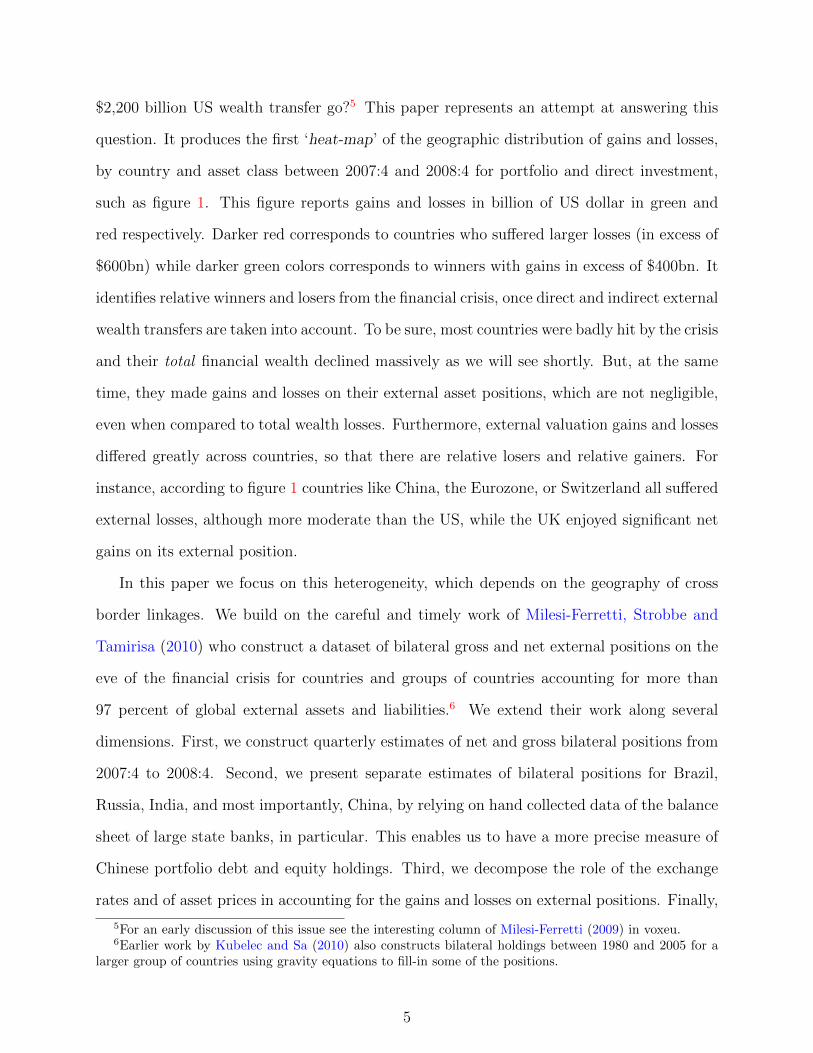
$2,200 billion US wealth transfer go?5 This paper represents an attempt at answering this

question. It produces the first ‘heat-map’ of the geographic distribution of gains and losses,

by country and asset class between 2007:4 and 2008:4 for portfolio and direct investment,

such as figure 1. This figure reports gains and losses in billion of US dollar in green and

red respectively. Darker red corresponds to countries who suffered larger losses (in excess of

$600bn) while darker green colors corresponds to winners with gains in excess of $400bn. It

identifies relative winners and losers from the financial crisis, once direct and indirect external

wealth transfers are taken into account. To be sure, most countries were badly hit by the crisis

and their total financial wealth declined massively as we will see shortly. But, at the same

time, they made gains and losses on their external asset positions, which are not negligible,

even when compared to total wealth losses. Furthermore, external valuation gains and losses

differed greatly across countries, so that there are relative losers and relative gainers. For

instance, according to figure 1 countries like China, the Eurozone, or Switzerland all suffered

external losses, although more moderate than the US, while the UK enjoyed significant net

gains on its external position.

In this paper we focus on this heterogeneity, which depends on the geography of cross

border linkages. We build on the careful and timely work of Milesi-Ferretti, Strobbe and

Tamirisa (2010) who construct a dataset of bilateral gross and net external positions on the

eve of the financial crisis for countries and groups of countries accounting for more than

97 percent of global external assets and liabilities.6 We extend their work along several

dimensions. First, we construct quarterly estimates of net and gross bilateral positions from

2007:4 to 2008:4. Second, we present separate estimates of bilateral positions for Brazil,

Russia, India, and most importantly, China, by relying on hand collected data of the balance

sheet of large state banks, in particular. This enables us to have a more precise measure of

Chinese portfolio debt and equity holdings. Third, we decompose the role of the exchange

rates and of asset prices in accounting for the gains and losses on external positions. Finally,

5For an early discussion of this issue see the interesting column of Milesi-Ferretti (2009) in voxeu.6Earlier work by Kubelec and Sa (2010) also constructs bilateral holdings between 1980 and 2005 for a

larger group of countries using gravity equations to fill-in some of the positions.

5

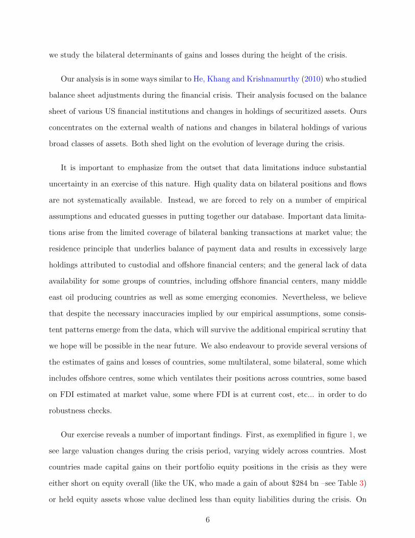
we study the bilateral determinants of gains and losses during the height of the crisis.

Our analysis is in some ways similar to He, Khang and Krishnamurthy (2010) who studied

balance sheet adjustments during the financial crisis. Their analysis focused on the balance

sheet of various US financial institutions and changes in holdings of securitized assets. Ours

concentrates on the external wealth of nations and changes in bilateral holdings of various

broad classes of assets. Both shed light on the evolution of leverage during the crisis.

It is important to emphasize from the outset that data limitations induce substantial

uncertainty in an exercise of this nature. High quality data on bilateral positions and flows

are not systematically available. Instead, we are forced to rely on a number of empirical

assumptions and educated guesses in putting together our database. Important data limita-

tions arise from the limited coverage of bilateral banking transactions at market value; the

residence principle that underlies balance of payment data and results in excessively large

holdings attributed to custodial and offshore financial centers; and the general lack of data

availability for some groups of countries, including offshore financial centers, many middle

east oil producing countries as well as some emerging economies. Nevertheless, we believe

that despite the necessary inaccuracies implied by our empirical assumptions, some consis-

tent patterns emerge from the data, which will survive the additional empirical scrutiny that

we hope will be possible in the near future. We also endeavour to provide several versions of

the estimates of gains and losses of countries, some multilateral, some bilateral, some which

includes offshore centres, some which ventilates their positions across countries, some based

on FDI estimated at market value, some where FDI is at current cost, etc... in order to do

robustness checks.

Our exercise reveals a number of important findings. First, as exemplified in figure 1, we

see large valuation changes during the crisis period, varying widely across countries. Most

countries made capital gains on their portfolio equity positions in the crisis as they were

either short on equity overall (like the UK, who made a gain of about $284 bn –see Table 3)

or held equity assets whose value declined less than equity liabilities during the crisis. On

6

the other side, taking the capital loss, is of course the US, who is long equity and made very

large losses on its portfolio equity position ($1,153bn, according to table 3). The structure of

the external debt portfolio, in particular whether debt assets are mostly government bonds

or corporate bonds or asset backed mortgage securities, is also a crucial determinant of the

valuation gains and losses. Countries who self-insured by holding mostly foreign government

bonds tended to limit their losses or even post gains on their net debt portfolios, while

countries who levered heavily to invest in risky asset backed mortgage securities or other

toxic assets experienced losses on their net debt. We find a clear positive correlation in the

data between the countries with losses on their net debt portfolios and those who set-up

ABCP conduits. Though the sample coverage is relatively small, we also find a positive

correlation between countries who set up ABCP conduits and the McGuire and von Peter

(2009) measure of US dollar shortage, suggesting that the lack of dollar liquidity in the

banking system was associated with important losses on external debt portfolios.

The next section reviews the evolution of the external balance sheets of the countries

in our sample, puts them in perspective by comparing them to changes in total wealth

of countries. We provide a world heatmap of external losses and decompose the effect of

exchange rates and asset prices on capital gains and losses. Section 3 discusses our empirical

methodology to construct bilateral gross and net positions for portfolio and direct asset

holdings, for which we have the most detailed data and presents the matrices of bilateral

gains and losses by asset class. Section 4 relates the distribution of wealth transfers to

observable determinants, such as the exposure to asset backed commercial paper (ABCP),

the overall dollar shortage as well as to measures of the regulatory environment. Section 5

concludes.

2 External Balance Sheet Adjustments

We begin our analysis by reviewing the evolution of the aggregate external balance sheet

for a large sample of countries from the end of 2007 to the end of 2008. This period covers

7

the most acute phase of the crisis during the fourth quarter of 2008 following the collapse of

Lehman Brothers, and is therefore the most relevant from the perspective of wealth transfers.

The recovery in many asset markets around the world in 2009 did reverse some of the

wealth transfers documented in this paper, perhaps as a result of the coordinated and ag-

gressive macroeconomic policies that may have helped stabilize the world economy. What

interests us here is a measure of the external wealth transfers resulting directly from the

crisis itself, i.e. measured at a time when the possibility and the effectiveness of coordinated

countercyclical policies remained remote and the risk of a second Great Depression was on

everyone’s mind. It would be interesting to quantify the impact of these external transfers

on the recovery path of the real economy across countries. Such an enterprise however goes

well beyond the current paper. One difficulty consists in controlling for the relative size

of the shocks hitting the various economies. Another lies in the endogeneity of the policy

responses. Instead, this paper focuses on the determinants of the relative gains and losses

on the external positions of countries and put those valuations in perspective by comparing

them to the contemporaneous changes in domestic household wealth.

2.1 Data and Methodology

Our sample includes most industrial countries (Canada, the Euro area, Japan, Switzerland,

the UK, the US), a group of other advanced economies (Australia, Denmark, New Zealand,

Norway and Sweden), some major emerging economies (Brazil, China, India, Russia, Singa-

pore, Hong-Kong) and a group of emerging Asian economies composed of Indonesia, South

Korea, Malaysia, the Philippines and Thailand. Missing from this sample are oil exporters

and offshore financial centers, both with potentially large gross and net cross-border posi-

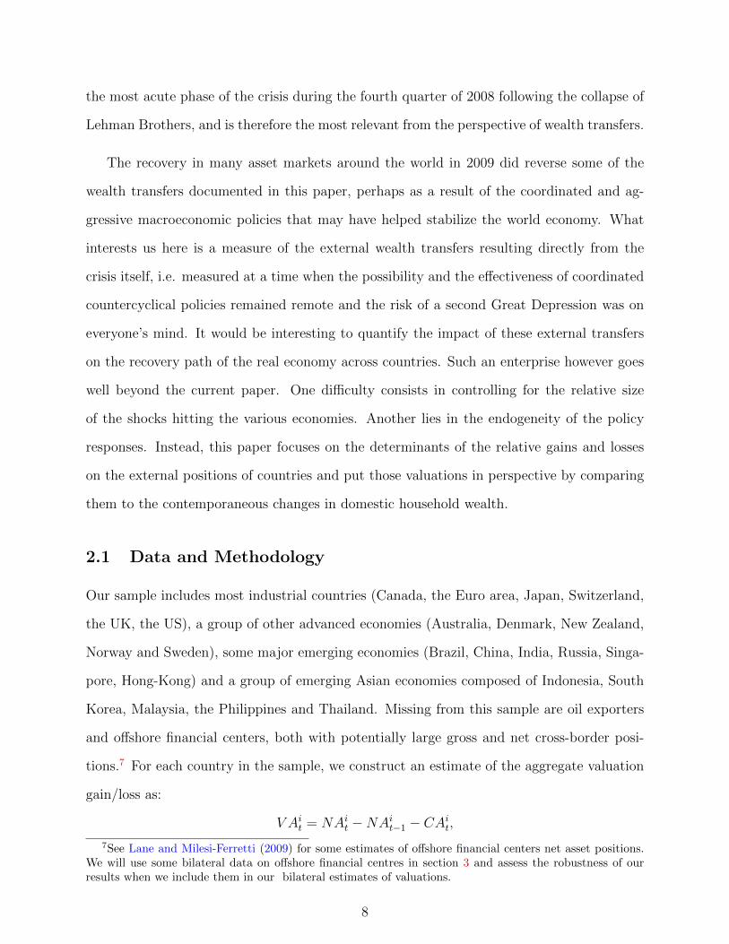
tions.7 For each country in the sample, we construct an estimate of the aggregate valuation

gain/loss as:

V Ait = NAi

t −NAit−1 − CAi

t,

7See Lane and Milesi-Ferretti (2009) for some estimates of offshore financial centers net asset positions.We will use some bilateral data on offshore financial centres in section 3 and assess the robustness of ourresults when we include them in our bilateral estimates of valuations.

8

where NAit denotes the net foreign asset position at time t for country i and CAi

t the current

account balance during period t. We further break down the net foreign asset position into

net direct investment, equity, portfolio debt and other assets (mostly bank loans), according

to NAit =

∑cNA

i,ct where NAi,c

t represents the net position of country i in asset class c at

time t. Using the balance of payment identity, we can write the valuation term as the sum of

the changes in the net asset position by asset classes, ∆NAi,ct , corrected for the net financial

flows in asset category c over the period, denoted NF i,ct .8

V Ait =

∑c

∆NAi,ct −NF i,c

t . (1)

2.2 Aggregate gains and losses

We collect quarterly and annual data on foreign assets and liabilities, at market value when-

ever possible, with corresponding financial flows, for this set of 11 individual countries and

3 country groups between 2007 and 2009. Assets and liabilities positions are broken down

into the following assets classes: portfolio debt, portfolio equity, direct investment, other in-

vestment and reserves (with matching flows, but excluding financial derivatives). For debt,

equity, direct investment and other investment positions we rely on national sources for

Canada, China, the Euro Area, Japan, Switzerland, United Kingdom and the United States

whereas for all other countries, data are from the IMF Balance of Payments Statistics. For

reserves we use “Total reserves minus gold” obtained from the IMF International Financial

Statistics. All flow data were obtained from the IMF Balance of Payments Statistics.9

We first offer a geographical ‘heatmap’ of aggregate gains and losses around the globe

in figure 1. As mentioned previously, countries with darker red colors bear the larger losses

(in excess of $600bn). The lighter red color represents smaller losses. Similarly, countries

with dark green color enjoyed the largest gains (in excess of $400 bn) while lighter green

represents smaller gains. Countries in plain white, such as, for example, African countries,

8The sum of net financial flows equals the current account balance, up to errors and omissions andunilateral transfers and remittances, which we ignore in this decomposition.

9For more details on our data see the Appendix.

9

are those for which we have no data. At a glance, we can see that most of the external

valuation losses are spread across the US, the Euro Area, Switzerland and China (Australia

and other advanced economies made very moderate losses). The UK on the other hand is at

the other end of the spectrum and made large capital gains on its net external asset position,

while Brazil, Russia and India made moderate gains.

Table 3 reports the corresponding numerical estimates (all the numbers are in billions of

US$) and figures 2-3 present the corresponding heatmap for each asset class (debt, equity,

FDI and foreign exchange) with the same color coding. Finally, figure 4 reports the break-

down of gains/losses by asset class and country. For each country, or group of countries,

this last figure reports V Ait (the solid line) as well as the various components ∆NAic

t −NF ict

according to equation (1).10

Figure 4 also includes the valuation gain/loss for the ‘rest of the world’ (RoW), defined as

the counterpart of the aggregate valuation term in our data: V Arowt = −

∑i V A

it. This valu-

ation term accounts both for incomplete geographical coverage as well as any measurement

error. Accordingly, its interpretation should be subject to extra caution.

For the purpose of comparability across countries, we constructed figure 4 and Table 3

with US direct investment positions measured at current cost. This brings down the overall

US valuation loss between 2007:4 and 2008:4 from -$2,069bn when using direct investment

at market value as in Table 1 and 2, to -$863bn.11.

A number of important features emerge from the data. First, the simple proposition that

the US suffered a valuation loss while other countries gained uniformly is not supported by

the data. The Euro area, mainland China and Switzerland all experienced sizeable losses, of

$185bn, $158bn and $53bn respectively whereas the UK ($542bn), Russia ($317bn), Brazil

($292bn) and emerging Asia ($245bn) were the main net beneficiaries. Taken together, the

countries of our sample –outside the US– experienced a positive wealth transfer of $1,145bn

10For table 3 and 4 we grouped debt and foreign exchange reserves in the debt category.11The valuation component on US net direct investment at market value is -$1,150bn and $56bn at current

cost. By construction, the difference, equal to $1,206bn, must be accounted for by valuation gains on netdirect investment (at market value) in other countries. The next section will provide rough estimates ofbilateral direct investment positions at market value.

10

exceeding the $863bn losses of the U.S., the difference being attributed to the rest of the

world.

Second, most of the US losses arise from the $1,153bn decline in its net equity portfolio.

By construction, the cross section distribution of valuations within each asset class sums to

zero, that is for each asset class c: ∑i

V Ai,ct = 0,

where V Ai,ct = ∆NAi,c

t −NF i,ct . Inspection of table 3 and figure 4 reveals that the counterpart

of the US net equity losses were widely distributed, most countries realizing gains on their

equity portfolio, especially the Euro area ($506bn), the UK ($284bn), Russia ($208bn), Brazil

($205bn), emerging Asia ($192bn) and Japan ($176bn). In all these countries, the gains arise

from a drastic reduction in the value of equity liabilities, relative to equity holdings. All these

countries had short cross border equity positions as of 2007.

Third, the gains/losses attributable to US cross-border portfolio debt holdings are rela-

tively small, all of the increase in debt liabilities ($505bn) being more than accounted for by

gross capital inflows ($591bn) especially into US government securities. The small associ-

ated valuation loss on US portfolio debt liabilities (-$86bn) underlies the relative stability of

U.S. government securities during the crisis. By contrast, the U.K., experienced a valuation

gain of $339bn on its net debt position, largely due to the decline in the value of its debt

liabilities (-$515bn), some of which can be attributed to the decline in the value of the Ster-

ling relative to the US dollar during that period. Conversely, the Euro area suffered large

valuation losses on its external debt claims (-$461bn) most likely related to the collapse in

the value of its portfolio of US structured credit products. Overall, the contrast between

these three countries is consistent with the US issuing safe public debt and risky private-label

debt (see Bernanke et al. (2011)); the Euro area holding a portfolio of risky private-label

debt assets; the U.K. issuing Sterling denominated debt and risky private-label debt both of

which declined in value during the crisis.

11

Fourth, despite large holdings of U.S. public securities China suffered an overall negative

wealth transfer during the crisis ($158bn), representing about 3.5 percent of its output.

China also suffered a $61bn loss on its foreign exchange reserve holdings, as a result of

the markdown on its non-dollar reserves when most currencies lost ground against the US

dollar.12 13. These findings highlight that the decline in China’s net external wealth would

have been much more pronounced, were it not for its large holdings of US government

securities.

Taken together, the results from table 3 and figure 4 reveal a remarkable pattern. If

we define ex-post global insurers as the set of countries that provided significant positive

transfers to the rest of the world during the financial crisis, this set includes the following

countries: the United States ($863bn, 6 percent of GDP), the Euro area ($185bn, 1.36

percent of GDP), Switzerland ($53bn, 10.6 percent of GDP) and China ($158bn, 3.5 percent

of GDP).14 The channels through which each of these countries experienced valuation losses

vary. For the US, it is the collapse in its long net equity position, relative to its short debt

position, which did not decline nearly as much. For Switzerland and the Euro area, it is

the decline in the value of their debt holdings, which were infested by toxic assets, and the

decline in the value of their long direct investment position. For China, as discussed above,

it is the losses on the non-dollar components of its foreign exchange reserves, due to a dollar

appreciation.

These findings indicate that the heatmap of gains and losses is substantially more complex

than expected. In particular, it suggests that it is incorrect to think of the United States as

12We measure gains and losses in dollars. If we measured valuation effects in a currency basket instead,such as the SDR, China would record a gain of about 2.6 bn SDR on its official foreign exchange holdings,as the SDR depreciated against the dollar at the height of the crisis. Except for this ”level effect” the choiceof a numeraire has no consequence on our results.

13The official IIP figures also indicate increases in the value of Chinese FDI and equity liabilities. Thesenumbers are however not at market value. Given that the Chinese stock market suffered a massive declineduring the crisis, Chinese liabilities are likely to be overstated in official IIP data. Hence, Chinese losses arelikely to be also overstated. In the next section of the paper we discuss in more details the shortcomings ofChinese data.

14Technically, the list should also include Singapore ($56bn valuation loss representing 29 percent of itsoutput). However, Singapore is a regional financial center and discrepancies between claims and liabilitieslead to us to interpret these numbers with caution.

12

the single provider of global liquidity. The allocation of losses is still extremely asymmetric

–with the US accounting for about 68 percent of the cross border wealth losses, the Euro

area for 15 percent, China for 13 percent and Switzerland for 4 percent.15 Nevertheless

it provides perhaps an early indication that the global economy may have already moved

towards a multilateral system, where the provision of global liquidity is not concentrated in

the hands of the United States any longer. On the whole, our results are also consistent with

the recent work emphasizing the resilience of emerging economies during the recent crisis

(see Kose and Prasad (2010) and Gourinchas and Obstfeld (2011)).

2.3 Exchange rate accounting, total wealth and valuations

The crisis period has been characterized by large gyrations in exchange rates, with, in par-

ticular a substantial appreciation of the dollar against most currencies. It is interesting

to decompose gains and losses on external balance sheets into fluctuations in asset prices

(equity, FDI, bond prices) and exchange rate movements. We attempt here such an account-

ing exercise in order to assess how much exchange rate movements explain our change in

valuations.

We use the geographical distribution of bilateral weights of assets and liabilities as well as

some crude assumptions on their currency composition to compute the relevant exchange rate

movements. In particular, we assume that all FDI and equities holdings are in the currency

of the issuer and that all bank loans are fully hedged and hence immune to exchange rate

effects. We use the Lane and Shambaugh’s exchange rate weights for the debt data.16

Our results presented in table 4 have striking features. All the countries we identified

15For the reasons mentioned above and discussed in more details below, the numbers for China are likelyto be very imprecise. The share of the US losses in total losses would be even larger if we measured directinvestment at market value since the US valuation loss would be roughly three times as large.

16In our benchmark case, we assume that all the assets that our source countries own in offshore centersare in US dollars. This may be a problematic assumption for some of our countries, like the UK, which havesusbstantial links with offshore centres and is likely to use sterling for at least part of these transactions. Asa robustness check, we assumed that all the UK assets vis-a-vis all offshore centers are in Sterling. The onlylarge difference is for the exchange rate valuation on FDI assets: instead of incurring a loss of $80 bn, theUK would incur a loss of $156 bn. While not negligible, this is unlikely to change our results in a materialway (UK offshore FDI assets are only 15% of total UK FDI assets).

13

in the previous section as ex post global insurers (US, Euro Area, Switzerland, China and

Singapore, with the addition of Japan) suffered valuation losses due to adverse exchange rate

movements. These are countries whose currencies have tended to hold rather well or even to

appreciate at the height of the crisis mainly due to their role as safe havens. Liabilities of

these countries are mainly in domestic currency and their assets mainly in foreign currencies,

hence an appreciation of the domestic exchange rate tends to decrease the value of their net

foreign assets. Our table shows that exchange rate movements account for about 31% of

US external valuation changes (when US FDI is measured at market value). This sizable

number (corresponding to a valuation loss of about $650 bn) is not surprising as the currency

composition of US external assets and liabilities is very asymmetric: almost all US liabilities

are in dollars while about two thirds of US assets are in foreign currencies. As the dollar

appreciated sharply in 2008 in part due to inflows into the Treasuries market, the value of

US external claims went down. For Switzerland and Japan, the losses stemming from the

strength of their currencies were partly compensated by an increase in the value of their

external claims. Both Switzerland and Japan have short equity positions and benefit from a

collapse in equity prices. A contrario, the Sterling collapse led to large exchange rate gains

on the UK net external positions. Those gains explain 139% of the total valuation changes,

meaning that they were partly offset by decreases in the value of UK net external assets

One legitimate question to ask is whether the international wealth transfers this paper

focuses on are relevant compared to the change in domestic financial wealth that occurred

during the crisis. We report in table 4 (columns (7) and (8)) changes in total domestic

household wealth for the subset of countries for which we could find data.17 First, declines

in wealth are indeed very large during the period we consider: $17.3 trillion for the United

States, $2.7 trillion for the UK and $2.3 trillion for Japan, $1.3 trillion for the Eurozone.

This should come as no surprise as our period spans the height of the financial crisis during

which many financial and real estate markets performed dismally. External valuation gains

17Source: OECD Economic Outlook (2011). Our data cover the US, the UK, the Euro Area (limited hereto Germany, Italy and France), Japan and Canada.

14

or losses, though smaller, are nevertheless quite sizeable as a proportion of total wealth

changes. Their absolute value range from 3% (for Japan) to 20% for the UK, reflecting both

the openness of the UK as a small open economy and the important role of London as an

international financial centre. For the US, external valuation changes amount to 12% of

the change in total household wealth, and for the Euro Area 14%. Hence, while there is

no doubt the negative domestic wealth effects dominate the macroeconomic landscape for

most of our countries, the international wealth transfers, determined by the heterogeneity of

external balance sheets, are far from being negligible.

3 Bilateral valuation gains and losses

Our world maps showed considerable geographical heterogeneity in external wealth changes

at the country level. We now refine our analysis and estimate the distributions of bilateral

valuations gains and losses during 2007-2008. Balance of payment data and international

investment positions are based on the concept of residency. This concept is not fully adequate

to analyze risk sharing in the international economy. Ideally, we would like to have data on

final ownership of assets. These data do not exist for portfolio investment or FDI however,

for which we will have to assume that residency and ownership coincide. The presence of

important financial links with offshore financial centres, which act merely as intermediate

financial platforms distort further the geographical picture of our data.18 All our results are

therefore subjected to these limitations. A second important difficulty is the estimation of

bilateral investment positions and bilateral flows in different asset classes. Kubelec and Sa

(2010) and Milesi-Ferretti, Strobbe and Tamirisa (2010) have done pioneering work in trying

to estimate bilateral investment positions. Nevertheless, data limitations remain severe in

terms of country coverage in particular and availability of data at market value (see the

appendix for a more detailed discussion of data issues).19

18For an attempt to assess the robustness of our results to the inclusion of offshore centres, see next section.19We chose not to compute bilateral financial matrices for bank loans. The locational banking statistics

of the BIS, based on the concept of residency, give data on bilateral banking positions. These data however

15

3.1 Data and Methodology

For each asset class, we estimate the bilateral distribution of valuation gains and losses

V X ijt+1 at time t + 1 between country i and j during the height of the crisis between 2007

Q4 and 2008 Q4. We derive V X ijt+1using the following accounting identity:

V X ijt+1 = PX ij

t+1 − PX ijt − FX ij

t+1, (2)

where PX ijt denotes the holdings of country i in country j at time t, and FX ij

t represents

the net financial purchases by residents of country i in country j in the asset class considered

between t and t+ 1.

Yearly data on some components of bilateral international portfolios holdings by asset

classes are available through the CPIS survey and other sources in recent years for a number

of countries. Bilateral flow data coverage is, however, generally far from complete or not

available. We use the following methodology to estimate bilateral flows on quarterly data.20

Portfolio debt and portfolio equity

We compute the bilateral portfolio weights wijt of country i vis-a-vis country j for a given

asset class at date t using bilateral CPIS data as: wijt = PX ij

t /∑

j∈CPIS

PX ijt . The coverage of

the CPIS data is not exhaustive, hence the sum of all the bilateral positions of country i for

portfolio debt or equity covered by the CPIS does not correspond to the reported aggregated

IIP for these assets. Accordingly, we construct a coverage rate for country i at date t as

αit =

∑j∈CPIS

PX ijt /PX

it , where PX i

t is the reported aggregate (multilateral) international

investment position for country i.21 We denote the aggregate flow in a given asset class by

are bound to be of little use for our purposes as loan books and large parts of the banking books are notmarked to market. The speed of write downs and the provisioning for bad loans have differed widely acrosscountries and it is unclear how much of this is reflected in the BIS numbers of 2007-2008. Furthermore, thereare large differences between consolidated statistics and locational statistics, suggesting that the concept ofresidency, compatible with balance of payment accounting is bound to be very different from the ultimategeographical distribution of gains and losses. Rather than attempt a heroic effort at reconciling loan dataon a bilateral basis, we preferred not to do bilateral financial matrices for this asset category.

20We provide all our data sources for specific countries in the appendix. When CPIS data are not available(as in the case of China) we use national data sources.

21We make sure that the valuation methods for the numerator and the denominator are the same.

16

FX it+1, and estimated variables with a ‘hat’. Our goal is to construct an estimate of the

quarterly bilateral flows FX ijt . Our working assumption is that the geographical distribution

of flows over each quarter corresponds to the portfolio weights at the beginning of the quarter.

Scaling total flows in proportion to the data coverage on the positions, it results that our

estimated bilateral flows are constructed as:

FX ijt+1 = wij

t FX it+1 α

it.

An estimate of next quarter’s positions (ex-valuation gains) can then be constructed as:

PX ijt+1 = PX ij

t + FX ijt+1

The procedure is then iterated by defining the next quarter portfolio weights as wijt+1 =

PX ijt+1/

∑j∈CPIS

PX ijt+1 and using these to construct the following quarter bilateral flows etc...

We recover the yearly valuation term in the fourth quarter, V X ijt+4, as the difference

between end of year bilateral positions as recorded in the available surveys, adjusted for our

constructed cumulated bilateral flows:

V X ijt+4 = PX ij

t+4 −4∑

s=1

FX ijt+s − PX ij

t

V X ijt+4 = PX ij

t+4 − αit

4∑s=1

wijt+s−1FX

it+s − PX ij

t ,

where the second line substitutes FX ijt+s for its empirical counterpart. We emphasize again

that this approach is quite crude, given the data limitation and is likely to suffer from a

number of shortcomings. However, in the absence of more detailed data, it strikes us as

reasonable to assume that flows are allocated proportionally to observed positions.22

22One simple case where our assumption would be violated is one where investors would want to maintainfixed portfolios shares. In that case, investors would rebalance fully their portfolio every period, which wouldrequire underweighting assets that outperform, so that the financial flows would not be exactly proportionalto beginning of period holdings. Our rule assumes that investors do not follow such a simple, full rebalancingrule; indeed at the observed frequencies, portfolio weights are time varying.

17

Bilateral FDI

For our sample, up-to-date official data on FDI at market value is only available for the

following countries: the US, Hong Kong, Japan, Australia and Sweden.23 In order to obtain

bilateral FDI positions at market value we rely wherever possible on official estimates of the

aggregate FDI positions at market value. For countries that do not report such estimates,

we update an initial market value estimate by using equity price indices and aggregate FDI

flows. Once we have the derived - or provided - estimate of the aggregate market value FDI

stock for 2007 and 2008, we use the ratio of market value to book value of the aggregate

stock to infer the bilateral FDI stocks at market value.

For the US, the BEA provides market value of the aggregate FDI stock which we use

to convert the bilateral BEA FDI positions at historical cost to market value. The same

method is used for Japan (where market value estimates are provided by the Bank of Japan)

and Sweden (with data from the Swedish Rijksbank).

For the UK, Switzerland, Denmark, Canada and China we rely on an initial estimate of

the aggregate FDI positions at market value which we update by using destination coun-

try equity indices and aggregate direct investment flows. We rely on Kubelec, Orskaug and

Tanaka (2007) for UK direct investment positions as of 2005; Kumah, Damgaard and Elkjaer

(2009) for Denmark in 2006; Stoffes and Tille (2009) for Switzerland in 2005 and Statistics

Canada for Canada in 2005 (see the appendix for a more detailed discussion of our mar-

ket value estimation methodology). For the remaining countries in our sample we rely on

bilateral DI positions at market value derived from partner countries sources. With these

estimates of yearly positions in hand, we construct bilateral FDI flows and valuations using

the same approach as for portfolio debt and equity.

Bilateral Foreign exchange data

For the currency composition of foreign exchange reserves we use national sources (Canada,

Russia, Switzerland and the UK) or else adopt the 2007 currency share of official reserves

23Of those, only Australia and Hong-Kong use market value as the primary FDI valuation method in theirofficial IIP release.

18

provided in Milesi-Ferretti, Strobbe and Tamirisa (2010) for 2008. For China, the currency

composition of reserves is usually not disclosed. We use the 2010 weights, as this is the only

year for which data are available. While this strategy is by no means optimal, we believe any

resulting errors to be comparatively small, in view of the relative stability of foreign reserve

currency shares over time.

Bilateral FX reserves valuations are computed using exchange rate movements applied

to the currency composition of reserves. We prefer this direct valuation method as flows

are bound to be very badly observed (reserve flows are kept confidential by some countries),

while exchange rate movements and currency composition are relatively accurate.

Treatment of offshore financial centres

The main offshore centres are in our sample.24 Though the reporting is spotty (see

Lane and Milesi-Ferretti (2009) for a thorough study) there are some important cross border

positions between some offshore centres (such as the Cayman Islands and the Bahamas, for

example) and advanced economies. It is very unlikely that the ultimate owners of financial

assets bought by offshore centres are actual residents of off-shore centres. Rather, offshore

centres act as intermediaries to channel funds across the globe, reflecting, among other things,

tax “optimization” and tax evasion. Zucman (2011) shows that a significant amount of rich

countries wealth seem to evaporate via those channels.

Because, by design, the traceability of the geography of financial flows emanating from

and going into offshore centres is limited, we make two different assumptions in the course

of our analysis and investigate the robustness of our results. First we simply take the

offshore centres out of the bilateral financial matrices. This means that we focus only on

the financial linkages across countries that are explicitly (even if imperfectly) recorded in

official data. Second, we assume that the bulk of offshore financial transactions is done to

go around domestic fiscal authorities, legally or illegally. Hence most of those transactions

are really domestic transactions intermediated offshore. We therefore redistribute offshore

24These include Aruba, Andorra, Bahamas, Barbados, Bermuda, British Virgin Islands, Cayman Islands,Gibraltar, Guernsey, Isle of Man, Jersey, Lebanon, Liechtenstein, Macao, Mauritius, Monaco, NetherlandAntilles, Panama, Samoa, San Marino, Vanuatu, Vatican, West Indies

19

centres external assets and liabilities to the other countries of our samples in the following

way. Take the US-Bahamas example. We assume that part of the external assets of the US

towards the Bahamas are actually US-US investments and we ventilate the rest according

to the weights of the US portfolio on external assets. Specifically we use the home bias of

the US equity portfolio to determine how many US-Bahamas claims are really US domestic

claims. On the liability side, we do a similar breakdown: US liabilities vis-a-vis the Bahamas

are assumed to be US-US liabilities (same home bias weight) and the remainder is ventilated

according to the weights in the US external liability portfolio.25

While these assumptions on offshore centers have some effect on the results, especially for

the countries which trade most with offshore centers, such as the US, the UK and the euro

area, the overall pattern of transfers does not change, whether in the aggregate or by asset

classes.26 We conclude that while there is no denying offshore centres introduce some degree

of uncertainty in the geographical distribution of gains and losses, the relative magnitudes

are such that they probably are not large enough to significantly alter our global heatmaps.

3.2 Bilateral Financial Matrices

Traditionally, the propensity of countries to experience a financial crisis has been linked

to large current account deficits and net imbalances. As financial globalization proceeds,

cross border asset positions are growing at a rapid rate, and balance sheet effects are be-

coming increasingly important: even countries with net balanced positions and no current

account deficit can become financially illiquid. Nowadays, financial fragility has to be as-

sessed through information on gross external asset positions, disaggregated by asset classes.

Tracking the process of international transmission of financial shocks involves knowing the

network of bilateral gross exposures of countries. Hence, we believe that the construction of

bilateral matrices such as the ones we are presenting in this paper for the 2007-2008 crisis,

25The home bias weights for equity and bonds are taken from Coeurdacier and Rey (2010). For FDI, weuse the same home bias weights as for the equity portfolio.

26Bilateral financial matrices with ventilation of offshore positions are not reported here due to lack ofspace. They are available upon request.

20

can be of great interest to understand better systemic risk and the propagation of shocks at

the international level. In what follows we present bilateral financial matrices on gains and

losses by asset categories (portfolio debt, equity and FDI).

There are several ways of constructing valuation matrices. We can use data on bilateral

assets and liabilities of reporting countries or alternatively use data based only on the asset

side of reporting countries. Because data on the asset side is usually more reliable (see

Milesi-Ferretti, Strobbe and Tamirisa (2010) for a discussion), this is what we present in this

section.

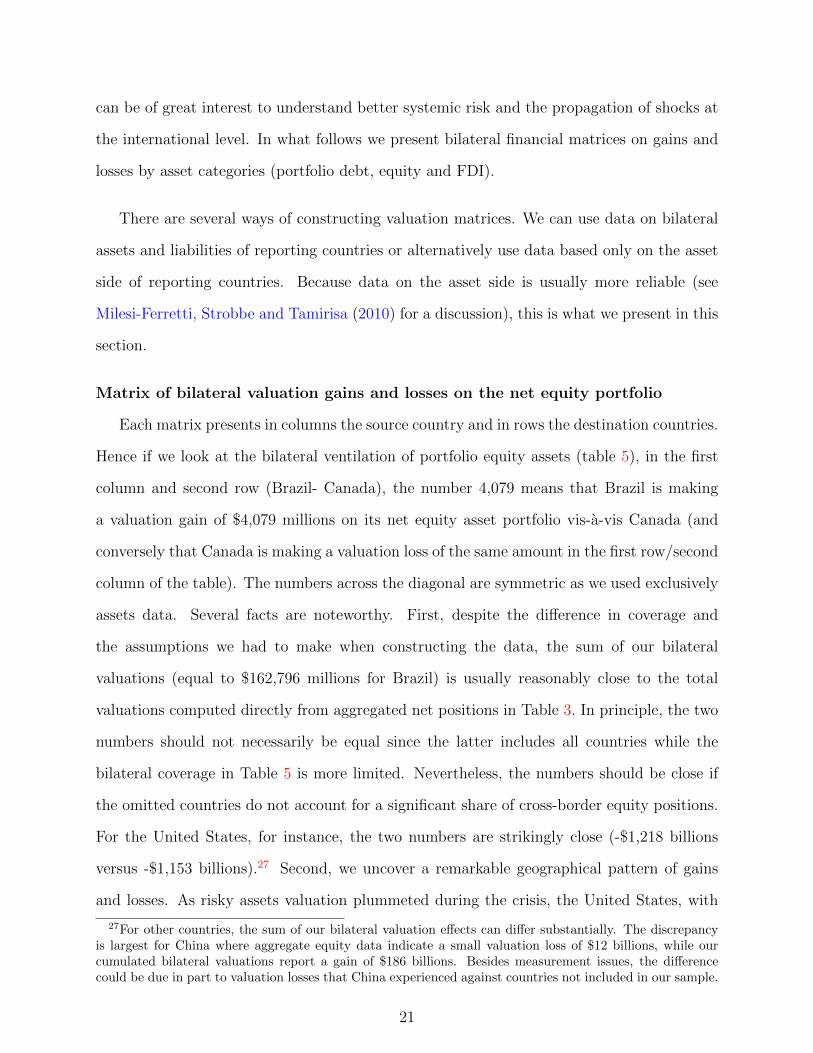
Matrix of bilateral valuation gains and losses on the net equity portfolio

Each matrix presents in columns the source country and in rows the destination countries.

Hence if we look at the bilateral ventilation of portfolio equity assets (table 5), in the first

column and second row (Brazil- Canada), the number 4,079 means that Brazil is making

a valuation gain of $4,079 millions on its net equity asset portfolio vis-a-vis Canada (and

conversely that Canada is making a valuation loss of the same amount in the first row/second

column of the table). The numbers across the diagonal are symmetric as we used exclusively

assets data. Several facts are noteworthy. First, despite the difference in coverage and

the assumptions we had to make when constructing the data, the sum of our bilateral

valuations (equal to $162,796 millions for Brazil) is usually reasonably close to the total

valuations computed directly from aggregated net positions in Table 3. In principle, the two

numbers should not necessarily be equal since the latter includes all countries while the

bilateral coverage in Table 5 is more limited. Nevertheless, the numbers should be close if

the omitted countries do not account for a significant share of cross-border equity positions.

For the United States, for instance, the two numbers are strikingly close (-$1,218 billions

versus -$1,153 billions).27 Second, we uncover a remarkable geographical pattern of gains

and losses. As risky assets valuation plummeted during the crisis, the United States, with

27For other countries, the sum of our bilateral valuation effects can differ substantially. The discrepancyis largest for China where aggregate equity data indicate a small valuation loss of $12 billions, while ourcumulated bilateral valuations report a gain of $186 billions. Besides measurement issues, the differencecould be due in part to valuation losses that China experienced against countries not included in our sample.

21

long equity positions vis-a-vis each of the other geographical entities in our sample, suffered

across the board losses. Furthermore, after controlling for their bilateral equity portfolio

gain against the US, all other advanced economies except Japan also made losses on their

net equity position, reflecting their overall short equity position vis-a-vis the US and long

position against the rest of the world. The case of the UK is particularly interesting. It

registers one of the biggest gain on its portfolio equity ($198 billions) and is characterized

by a massive short position vis-a-vis the US and a somewhat smaller short position vis-a-vis

the Euro Area and Canada. Emerging markets, on the other hand, tend to be short equity

vis-a-vis most of their partners, and as a result, benefited from the worldwide fall in equity

markets. This is particularly clear for the BRIC countries (Brazil, Russia, India and China)

who make gains on most of their bilateral net equity positions.

Matrix of bilateral valuation gains and losses on the net debt portfolio.

The data on portfolio debt presented in table 6 show bigger gaps in coverage than the

equity data. In particular, the data coverage for the Euro area and the UK seems particularly

limited, as revealed by the comparison between the sum of bilateral gains and losses and the

aggregate figure obtained directly from the IIP in Table 3. Data coverage for the United

States seems adequate since we report a valuation loss of $58 billions while the aggregate

position indicates $46 billions. It would be ideal to be able to distinguish between government

debt and corporate debt, including structured credit products Unfortunately this breakdown

is not available. Hence the net valuation on the debt portfolio will depend on the relative

weights of US treasuries, say, versus asset-backed mortgage securities in countries portfolios.

As indicated, our matrix also does not include official reserve holdings with the data on

debt (unlike Table 3 above which aggregated the two). According to Bernanke et al. (2011),

saving glut economies such as China and Emerging Asia have concentrated their portfolio

holdings into government bonds, pushing downwards their yields and inducing more advanced

economies, in particular the euro area to invest in higher yielding securities, such as ABCP.

Our data seem consistent with this narrative, as the Euro Area has a large long position in

US debt in 2007, which translated in large losses during the crisis. Similarly, other advanced

22

economies, Canada, Switzerland, who were also long in US debt and had presumably a

similar portfolio structure as the Euro area made losses on their net debt liabilities. A

noticeable exception is the UK, who, despite a long position in US debt realized a massive

gain, due mainly to the collapse of the value of US debt assets in the UK. The US makes gains

on its net debt portfolio vis-a-vis most advanced economies (except the UK) and conversely

makes losses vis-a-vis Russia and Hong Kong, which are likely to have accumulated more

US government bonds than corporate debt.

Matrix of bilateral valuation gains and losses on the net FDI portfolio

Comparing the sum of our bilateral net valuations for FDI at market value presented

in Table 7 with the aggregate data on valuation estimated from reported IIP, our data

coverage is clearly limited for some areas.28 The Euro area coverage in particular seems

most problematic, since the sum of bilateral valuations indicates a gain of $575 billions,

while the corresponding aggregate figure in Table 3 is a loss of $334 billions (based on FDI

at book value). It seems unlikely that the discrepancy, a valuation loss in excess of $1,000

billions, could be accounted for purely by the gaps in our geographic coverage, especially

vis-a-vis other emerging markets. With this caveat in mind, the results on bilateral direct

investment still present some interesting features. Japan has net DI assets vis-a-vis all the

countries in our sample, except Switzerland. Consequently, it suffered bilateral losses against

each country (except Switzerland and India). Similarly the US made large losses vis-a-vis

the Euro area against which it holds a large long position. UK FDI in the US seems to have

particularly underperformed and is responsible for the gain that the US makes on its net

FDI portfolio vis-a-vis the UK.

Matrix of bilateral valuation gains and losses on the foreign exchange reserves

Since the dollar is the dominant reserve currency, using the dollar as the numeraire would

28Note that for this matrix, we constructed market value FDI estimates wherever possible (see Appendix).Thus, the data presented here differs from the data presented in Table 3, where, e.g. for the US we used FDIat current cost to allow for better comparability across countries and, similarly, most other countries usebook values to compile their aggregate FDI data. In consequence, the sum of bilateral valuations in Table 7is not directly comparable with the aggregate figures in Table 3.

23

lead to many entries being zero.29 For this matrix (and only this one), we therefore chose

to express valuations in terms of the SDR basket in Table 8. For the 2006-2010 period, the

SDR weights were 44% dollar, 34% euro, 11% yen, 11% sterling. Since the SDR depreciated

against the US dollar and the yen in 2008, countries holding reserves predominantly in US $

and /or yen have seen their official reserves appreciate, when measured in SDR. For example,

China made moderate net gains on its foreign reserves during this period, because of the

strengthening of the dollar and the yen. China made some losses on its euro and, even

more sizably on its sterling reserves. Russia, on the other hand suffered net losses due to its

exposure to euro and sterling assets. So did the euro area, as it is heavily exposed to sterling

assets.

4 Determinants of gains and losses

It is now well understood that before the crisis, a number of AAA-rated securities (mostly

asset-backed mortgage securities) were perceived as perfect substitutes for US government

securities. Following Bernanke et al. (2011), let us call them ‘private-label’ safe assets. Even-

tually, the safety of the private label assets proved illusory, and their price spiralled down-

wards during the crisis. By contrast, US Treasuries held-up remarkably well and even saw

their price rise due to inflows of capital seeking safe haven protection (see McCauley and

McGuire (2009)). Acharya and Schnabl (2010) estimate that the banks around the world

manufactured over $1,200 billion of these ‘private-label’ safe assets by selling short-term

Asset-Backed Commercial Paper (ABCP) via conduits to risk-averse investors and investing

the proceeds primarily in long-term U.S. securities. As liquidity in the dollar money markets

dried-up in 2007, many banks found themselves unable to roll over these ABCP and forced

to reinstate the mortgages from the conduits on their balance sheet, with significant losses.

Bilateral exposure data are ideal to investigate the macroeconomic impact of those invest-

29We assume that currency and residency coincide, i.e. Chinese holdings of US$ reserves are assets ofChina on the US. As there are few reserve currencies, there are already a large number of zeros in thismatrix.

24

ments by commercial banks, i.e. whether countries whose banks set up large asset-backed

commercial paper conduits also experienced large losses on their external debt portfolios,

as measured by the “Survey on Portfolio holdings of U.S. Securities”. Figure 5 illustrates

the positive correlation between the share of ABCP conduits in total external debt positions

as of 2007 and the rate of losses made on external debt portfolios between 2007 Q4 and

2008 Q4.30 Though the sample is small, the correlation is strikingly positive, suggesting

that setting up ABCP conduits is a major determinant of aggregate losses on external debt.

Furthermore, there is a strong mapping between the geographical distributions of losses and

the share of the various areas in total ABCP holdings. As pointed out in Bernanke et al.

(2011), the Euro area leveraged massively to invest in those private-label safe assets ending

up holding 40% of total outstanding ABCP and as a result saw massive decline in the value

of its external debt to the tune of 54% of total losses (Figure 6). The UK, who held 16% of

the total stock of ABCP bore 21% of total losses.

Reinforcing the plausibility of the mechanism described above linking prevalence of ABCP

conduits and liquidity dry ups entailing losses on assets, we find a strong positive correlation

between the measures of dollar shortage in some banking systems developed by McGuire

and von Peter (2009) and the propensity of those systems to set up ABCP conduits. Figure

7 uses the upper limits of the dollar shortage measures developed by McGuire and von Peter

(2009) both at the office and at the group level. Those measures are constructed by assuming

that net interbank borrowing in dollar, net borrowing on the FX swap markets in dollars

(which the authors back out from the balance sheet identity assuming no open positions on

the forex), dollar borrowing from official monetary authorities, as well as liabilities to non

banks are all short term. The difference between those short term dollar liabilities and the

longer term dollar assets gives the dollar funding gap or dollar shortage of a country banking

system.31 With the exception of Switzerland, which did not appear to have any significant

30We are very grateful to Viral Acharya and Philip Schnabl for sharing their data with us. Their datasetconsists in the following countries: Australia, Austria, Belgium, Canada, Denmark, Frecnh, Germany, Italy,Japan, Netherthelands, spain, Sweden, Switzerland, UK, USA.

31We are grateful to the authors for providing us with their data, whose construction is described inMcGuire and von Peter (2009). The group-level estimates are constructed by aggregating banks’ global

25

exposure to ABCPs in 2007, there is a very clear link between measures of dollar shortage

and ABCP conduits.

Finally, we report in Figure 8 the total valuation losses together with the Kaufmann,

Kraay and Mastruzzi (2010) indicator of the quality of the regulatory environment. Recent

research by Giannone, Lenza and Reichlin (2011) finds that the severity of the crisis was

strongly and robustly positively related to the degree of liberalization in credit markets, as

measured by indicators or ‘regulatory quality’.32 In our sample, the correlation between

losses and the Kaufmann, Kraay and Mastruzzi (2010) indicator of the quality of the regu-

latory environment is also positive (0.45) and visual inspection confirms that countries with

more liberalized credit markets tended to suffer larger valuation losses on their external port-

folio. One may conjecture, that the most deregulated markets where also the ones in which

investors ”splurged” the most and increased their loadings on (once lucrative) toxic assets.

5 Conclusion

The global crisis of 2007-2009 led to massive changes in relative asset prices. We construct

a dataset that allows us to analyze the geography of wealth transfers during the crisis. The

‘heatmap’ we produce highlight a very diverse set of outcomes depending on the structure

of the structure of countries’ external portfolios. Some saw the value of their net assets

plunging, others benefited from large capital gains. The countries whose net international

asset positions deteriorated provided wealth transfers to the others at a time where marginal

utility of consumption was very high. For that reason they can be regarded as ”global

insurers”, as suggested in Gourinchas, Rey and Govillot (2010). Interestingly, we find that

the United States, the country at the centre of the international monetary system and issuer

balance sheets into a consolidated whole, and then calculating funding risk on this aggregated balance sheet.The office-level estimates are constructed by calculating funding risk at the office location level, and thenaggregating the series up across office locations for each banking system. By construction, the office levelestimates should at least be as large as the corresponding group level.

32For group of countries, we assign the regulatory quality index as follows: Germany for euro area, St Kittsfor offshore centers, Saudi Arabia for oil exporters, Thailand for emerging Asia, Norway for other advancedcountries, and Peru for other latin-american countries.

26

of the main reserve assets, the US Treasuries, provided most of the insurance during the crisis,

as its international investment position deteriorated massively. But other countries, which

may be regarded more like regional insurers joined in, such as Switzerland, the Euro area

or even China. A general pattern in our data is that most countries long equity or direct

investment faced losses on their net positions, as risky assets took some of the sharpest

valuation falls in the crisis. For portfolio debt, the exact structure of portfolio matters, and

in particular the relative weights of government bonds versus toxic corporate debt made

an important difference for the outcomes. We find that some correlation of exposure to

ABCP conduits -mostly in US dollars, existing dollar shortage measures, and losses on the

debt portfolio. Finally our exercise, just like Milesi-Ferretti, Strobbe and Tamirisa (2010)

underlines important data issues regarding cross country coverage of international investment

positions and flows.

27

References

Acharya, Viral V., and Philipp Schnabl. 2010. “Do Global Banks Spread Global Im-balances? Asset-Backed Commercial Paper during the Financial Crisis of 200709.” IMFEconomic Review, 58(1): 37–73.

Alogoskoufis, George, and Richard Portes. 1993. “Establishing a Central Bank: Issuesin Europe and Lessons from the US, Cambridge.” , ed. Matthew Canzoneri, Vittorio Grilliand Paul Masson, Chapter European Monetary Union and International Currencies in aTripolar World, 273–301. Cambridge University Press.

Bernanke, Ben S., Carol Bertaut, Laurie Pounder DeMarco, and Steven Kamin.2011. “International capital flows and the returns to safe assets in the United States, 2003-2007.” Board of Governors of the Federal Reserve System International Finance DiscussionPapers 1014.

Bertaut, Carol C., and Ralph W. Tryon. 2007. “Monthly estimates of U.S. cross-border securities positions.” Board of Governors of the Federal Reserve System (U.S.)International Finance Discussion Papers 910.

Bertaut, Carol, Laurie Pounder DeMarco, Steven Kamin, and Ralph Tryon. 2011.“ABS Inflows to the United States and the Global Financial Crisis.” Board of Governorsof the Federal Reserve System mimeo.

Coeurdacier, Nicolas, and Helene Rey. 2010. “Home Bias in Open Economy FinancialMacroeconomics.” London Business School 2011.

Cohen, Benjamin. 1971. The Future of Sterling as an International Currency. London:MacMillan.

Curcuru, Stephanie E., Tomas Dvorak, and Francis Warnock. 2008. “Cross-borderreturns differentials.” Quarterly Journal of Economics, 123(4): 1495–1530.

Forbes, Kristin J., and Francis E. Warnock. 2010. “Capital Flow Waves: Surges, Stops,Flight and Retrenchment.” MIT and University of Virginia mimeo.

Giannone, Domenico, Michele Lenza, and Lucrezia Reichlin. 2011. “Market Freedomand the Global Recession.” IMF Economic Review, 59(1): 111–135.

Gourinchas, Pierre-Olivier, and Helene Rey. 2007. “From World Banker to WorldVenture Capitalist: US External Adjustment and the Exorbitant Privilege.” 11–55.Chicago,:University of Chicago Press,.

Gourinchas, Pierre-Olivier, and Maurice Obstfeld. 2011. “Stories of the TwentiethCentury for the Twenty-First.” American Economic Journal: Macroeconomics, forthcom-ing.

Gourinchas, Pierre-Olivier, Helene Rey, and Nicolas Govillot. 2010. “ExorbitantPrivilege and Exorbitant Duty.” UC Berkeley mimeo.

28

Hartmann, Philip. 1998. Currency Competition and Foreign Exchange Markets: The Dol-lar, the Yen and the Euro. Cambridge University Press.

He, Zhiguo, In Gu Khang, and Arvind Krishnamurthy. 2010. “Balance Sheet Ad-justments during the 2008 Crisis.” IMF Economic Review, 58(1): 118–156.

Kaufmann, Daniel, Aart Kraay, and Massimo Mastruzzi. 2010. “The worldwide gov-ernance indicators : methodology and analytical issues.” The World Bank Policy ResearchWorking Paper Series 5430.

Kose, M. Ayhan, and Eswar S. Prasad. 2010. Emerging markets: Resilience and growthamid global turmoil. Washington, DC:Brookings Institution Press.

Krugman, Paul. 1984. Currencies and Crises. MIT Press.

Kubelec, Chris, and Filipa Goncalves Sa. 2010. “The geographical composition ofnational external balance sheets: 1980-2005.” Bank of England Bank of England workingpapers 384.

Kubelec, Chris, Bjorn-Erik Orskaug, and Misa Tanaka. 2007. “Financial Globali-sation, External Balance Sheets and Economic Adjustment.” Bank of England QuarterlyBulletin, 2: 244–57.

Kumah, Emmanuel, Jannick Damgaard, and Thomas Elkjaer. 2009. “Valuation ofUnlisted Direct Investment Equity.” International Monetary Fund IMF Working PaperWP/09/242.

Lane, Philip, and Gian Maria Milesi-Ferretti. 2009. “Cross-Border Investment in SmallInternational Financial Centers.” IIIS The Institute for International Integration StudiesDiscussion Paper Series iiisdp316.

Lane, Philip R., and Gian Maria Milesi-Ferretti. 2001. “The External Wealth of Na-tions: Measures of Foreign Assets and Liabilities for Industrial and Developing Countries.”Journal of International Economics, 55: 263–94.

Lane, Philip R., and Gian Maria Milesi-Ferretti. 2007. “The External Wealth ofNations Mark II: Revised and Extended Estimates of Foreign Assets and Liabilities, 1970-2004.” Journal of International Economics, 73(2): 223–250.

Matsuyama, Kiminori, Nobuhiro Kiyotaki, and Akihiro Matsui. 1993. “Toward aTheory of International Currency.” Review of Economic Studies, 60(2): 283–307.

McCauley, Robert N, and Patrick McGuire. 2009. “Dollar appreciation in 2008: safehaven, carry trades, dollar shortage and overhedging.” BIS Quarterly Review.

McGuire, Patrick, and Goetz von Peter. 2009. “The US dollar shortage in globalbanking.” BIS Quarterly Review.

McKinnon, Ronald. 1979. Money in International Exchange: The Convertible CurrencySystem. Oxford: Oxford University Press.

29

Mendoza, Enrique G., Vincenzo Quadrini, and Jose-Victor Rios-Rull. 2009. “Fi-nancial Integration, Financial Development, and Global Imbalances.” Journal of PoliticalEconomy, 117(3): 371–416.

Milesi-Ferretti, Gian-Maria. 2009. “A $2 trillion question.” http: // www. voxeu. org/

index. php? q= node/ 2902 .

Milesi-Ferretti, Gian-Maria, Francesco Strobbe, and Natalia Tamirisa. 2010. “Bi-lateral Financial Linkages and Global Imbalances: A View on The Eve of the FinancialCrisis.” CEPR Discussion Paper 8173.

Portes, Richard, and Helene Rey. 1998. “The Emergence of the Euro as an InternationalCurrency.” Economic Policy, 305–343.

Rey, Helene. 2001. “International Trade and Currency Exchange.” Review of EconomicStudies, 68(2): 443–464.

Simard, Eric, and Eric Boulay. “Market valuation of Equity in the International Invest-ment Position: Canada’s Experience.” Prepared for the Nineteenth Meeting of the IMFCommittee on Balance of Payments Statistics Frankfurt, Germany, October 23-26, 2006.

Stoffes, Nicolas, and Cedric Tille. 2009. “Where have the Savings gone to? Assessingthe Return on Switzerland’s External Assets.” Graduate Institute for International andDevelopment Studies working paper.

Zhou, Ruilin. 1997. “Currency Exchange in a Random Search Model.” Review of EconomicStudies, 64: 289–310.

Zucman, Garbiel. 2011. “The Missing Wealth of Nations: Are Europe and the U.S. netDebtors or net Creditors?” Paris School of Economics mimeo.

30

References

Acharya, Viral V., and Philipp Schnabl. 2010. “Do Global Banks Spread Global Im-balances? Asset-Backed Commercial Paper during the Financial Crisis of 200709.” IMFEconomic Review, 58(1): 37–73.

Alogoskoufis, George, and Richard Portes. 1993. “Establishing a Central Bank: Issuesin Europe and Lessons from the US, Cambridge.” , ed. Matthew Canzoneri, Vittorio Grilliand Paul Masson, Chapter European Monetary Union and International Currencies in aTripolar World, 273–301. Cambridge University Press.

Bernanke, Ben S., Carol Bertaut, Laurie Pounder DeMarco, and Steven Kamin.2011. “International capital flows and the returns to safe assets in the United States, 2003-2007.” Board of Governors of the Federal Reserve System International Finance DiscussionPapers 1014.

Bertaut, Carol C., and Ralph W. Tryon. 2007. “Monthly estimates of U.S. cross-border securities positions.” Board of Governors of the Federal Reserve System (U.S.)International Finance Discussion Papers 910.

Bertaut, Carol, Laurie Pounder DeMarco, Steven Kamin, and Ralph Tryon. 2011.“ABS Inflows to the United States and the Global Financial Crisis.” Board of Governorsof the Federal Reserve System mimeo.

Coeurdacier, Nicolas, and Helene Rey. 2010. “Home Bias in Open Economy FinancialMacroeconomics.” London Business School 2011.

Cohen, Benjamin. 1971. The Future of Sterling as an International Currency. London:MacMillan.

Curcuru, Stephanie E., Tomas Dvorak, and Francis Warnock. 2008. “Cross-borderreturns differentials.” Quarterly Journal of Economics, 123(4): 1495–1530.

Forbes, Kristin J., and Francis E. Warnock. 2010. “Capital Flow Waves: Surges, Stops,Flight and Retrenchment.” MIT and University of Virginia mimeo.

Giannone, Domenico, Michele Lenza, and Lucrezia Reichlin. 2011. “Market Freedomand the Global Recession.” IMF Economic Review, 59(1): 111–135.

Gourinchas, Pierre-Olivier, and Helene Rey. 2007. “From World Banker to WorldVenture Capitalist: US External Adjustment and the Exorbitant Privilege.” 11–55.Chicago,:University of Chicago Press,.

Gourinchas, Pierre-Olivier, and Maurice Obstfeld. 2011. “Stories of the TwentiethCentury for the Twenty-First.” American Economic Journal: Macroeconomics, forthcom-ing.

Gourinchas, Pierre-Olivier, Helene Rey, and Nicolas Govillot. 2010. “ExorbitantPrivilege and Exorbitant Duty.” UC Berkeley mimeo.

31

Hartmann, Philip. 1998. Currency Competition and Foreign Exchange Markets: The Dol-lar, the Yen and the Euro. Cambridge University Press.

He, Zhiguo, In Gu Khang, and Arvind Krishnamurthy. 2010. “Balance Sheet Ad-justments during the 2008 Crisis.” IMF Economic Review, 58(1): 118–156.

Kaufmann, Daniel, Aart Kraay, and Massimo Mastruzzi. 2010. “The worldwide gov-ernance indicators : methodology and analytical issues.” The World Bank Policy ResearchWorking Paper Series 5430.

Kose, M. Ayhan, and Eswar S. Prasad. 2010. Emerging markets: Resilience and growthamid global turmoil. Washington, DC:Brookings Institution Press.

Krugman, Paul. 1984. Currencies and Crises. MIT Press.

Kubelec, Chris, and Filipa Goncalves Sa. 2010. “The geographical composition ofnational external balance sheets: 1980-2005.” Bank of England Bank of England workingpapers 384.

Kubelec, Chris, Bjorn-Erik Orskaug, and Misa Tanaka. 2007. “Financial Globali-sation, External Balance Sheets and Economic Adjustment.” Bank of England QuarterlyBulletin, 2: 244–57.

Kumah, Emmanuel, Jannick Damgaard, and Thomas Elkjaer. 2009. “Valuation ofUnlisted Direct Investment Equity.” International Monetary Fund IMF Working PaperWP/09/242.

Lane, Philip, and Gian Maria Milesi-Ferretti. 2009. “Cross-Border Investment in SmallInternational Financial Centers.” IIIS The Institute for International Integration StudiesDiscussion Paper Series iiisdp316.

Lane, Philip R., and Gian Maria Milesi-Ferretti. 2001. “The External Wealth of Na-tions: Measures of Foreign Assets and Liabilities for Industrial and Developing Countries.”Journal of International Economics, 55: 263–94.

Lane, Philip R., and Gian Maria Milesi-Ferretti. 2007. “The External Wealth ofNations Mark II: Revised and Extended Estimates of Foreign Assets and Liabilities, 1970-2004.” Journal of International Economics, 73(2): 223–250.

Matsuyama, Kiminori, Nobuhiro Kiyotaki, and Akihiro Matsui. 1993. “Toward aTheory of International Currency.” Review of Economic Studies, 60(2): 283–307.

McCauley, Robert N, and Patrick McGuire. 2009. “Dollar appreciation in 2008: safehaven, carry trades, dollar shortage and overhedging.” BIS Quarterly Review.

McGuire, Patrick, and Goetz von Peter. 2009. “The US dollar shortage in globalbanking.” BIS Quarterly Review.

McKinnon, Ronald. 1979. Money in International Exchange: The Convertible CurrencySystem. Oxford: Oxford University Press.

32

Mendoza, Enrique G., Vincenzo Quadrini, and Jose-Victor Rios-Rull. 2009. “Fi-nancial Integration, Financial Development, and Global Imbalances.” Journal of PoliticalEconomy, 117(3): 371–416.

Milesi-Ferretti, Gian-Maria. 2009. “A $2 trillion question.” http: // www. voxeu. org/

index. php? q= node/ 2902 .

Milesi-Ferretti, Gian-Maria, Francesco Strobbe, and Natalia Tamirisa. 2010. “Bi-lateral Financial Linkages and Global Imbalances: A View on The Eve of the FinancialCrisis.” CEPR Discussion Paper 8173.

Portes, Richard, and Helene Rey. 1998. “The Emergence of the Euro as an InternationalCurrency.” Economic Policy, 305–343.

Rey, Helene. 2001. “International Trade and Currency Exchange.” Review of EconomicStudies, 68(2): 443–464.

Simard, Eric, and Eric Boulay. “Market valuation of Equity in the International Invest-ment Position: Canada’s Experience.” Prepared for the Nineteenth Meeting of the IMFCommittee on Balance of Payments Statistics Frankfurt, Germany, October 23-26, 2006.

Stoffes, Nicolas, and Cedric Tille. 2009. “Where have the Savings gone to? Assessingthe Return on Switzerland’s External Assets.” Graduate Institute for International andDevelopment Studies working paper.

Zhou, Ruilin. 1997. “Currency Exchange in a Random Search Model.” Review of EconomicStudies, 64: 289–310.

Zucman, Garbiel. 2011. “The Missing Wealth of Nations: Are Europe and the U.S. netDebtors or net Creditors?” Paris School of Economics mimeo.

33

1971:3 2007:2Gross Liabilities 11.2 130.8Bank Loans 3.1 38.8Debt 4.4 44.2of which:Government 3.7 21.2Corporate 0.8 23.1

Equity 2.6 22.2Direct Investment 1.2 25.6

Gross Asset 16.9 119.1Gold 1.1 1.2Bank Loans 5.3 36.1Debt 1.4 10.0Equity 0.7 35.0Direct Investment 8.4 36.5

Net 5.7 -11.7

Safe & Liquid/Liabilities 66.6 63.5Risky & Illiquid/Assets 53.9 60.0

Table 1: US External Balance Sheet, percent of US GDP. FDI at market value. Source:Gourinchas, Rey and Govillot (2010)

34

Positions as of: 2007:4 2009:1 Change% of GDP % of GDP bn (US dollars)

Net -10.2 -31.4 -21.1 -2,966of whichcumulated current account -5.5 -767valuation change -15.7 -2,199

Gross Liabilities 132.6 113.3 -21.6 -3,040Bank Loans 38.9 34.8 -4.8 -669Debt 46.0 48.8 2.1 288of which:Government 22.3 29.7 7.0 987Corporate 23.7 19.2 -5.0 -699

Equity 22.6 13.5 -9.5 -1,333Direct Investment 25.2 16.2 -9.4 -1,326

Gross Asset 122.5 81.8 -42.7 -6,006Gold 1.5 1.7 0.2 22Bank Loans 36.2 35.4 -1.4 -200Debt 11.1 8.8 -2.5 -353Equity 36.7 17.0 -20.4 -2,866Direct Investment 36.9 19.0 -18.6 -2,609

Table 2: Change in US External Balance Sheet. Percent of US GDP. 2007:4 to 2009:1. FDIat market value. Source: Gourinchas, Rey and Govillot (2010)

35

Val

uat

ion

Equit

yD

irec

tIn

vest

men

tD

ebt

Loa

ns

Cou

ntr

yC

laim

sL

iab.

Net

Cla

ims

Lia

bilit

yN

etC

laim

sL

iab.

Net

Cla

ims

Lia

b.

Net

U.S

.-8

63-2

,398

-1,2

45-1

,153

-161

-218

56-1

20-8

6-3

414

9-1

1926

8E

uro

area

-185

-1,1

71-1

,677

506

-607

-273

-334

-461

-135

-326

-394

-363

-31

U.K

.54

2-5

67-8

5128

4-4

23-3

37-8

6-1

76-5

1533

9-3

32-3

375

Jap

an65

-244

-420

176

746

-39

-66

126

-193

419

298

121

Sw

itze

rlan

d-5

3-1

97-2

2023

2877

-49

-45

-6-3

913

211

Can

ada

17-2

61-1

89-7

1-7

8-1

3153

-24

-41

18-7

-25

18O

ther

adva

nce

d-3

-434

-401

-33

-221

-234

14-1

35-1

428

-101

-111

10B

razi

l29

2-2

-207

205

7-6

774

8-1

523

-37

-9In

dia

200

-18

180

-24

24-2

50

-24

-1-3

3R

uss

ia31

7-1

-209

208

-220

-350

130

-18

-18

0-5

0-2

9-2

1E

mer

ging

Asi

a24

5-5

4-2

4619

2-1

0-6

757

-24

-8-1

6-3

5-4

813

Chin

a-1

581

13-1

216

64-4

8-6

1-2

-59

-22

17-3

9H

ong

Kon

g10

1-2

58-2

37-2

1-3

00-4

2112

27

25

-8-4

-4Sin

gap

ore

-56

-80

-74

-5-2

7-2

2-6

-31

0-3

1-1

50

-15

Res

tof

the

Wor

ld-2

82-3

1432

329

-329

Tab

le3:

The

Geo

grap

hy

ofW

ealt

hT

ransf

ers,

2007

:4-2

008:

4.D

ecom

pos

itio

nof

the

valu

atio

nch

ange

into

anet

equit

y,net

dir

ect

inve

stm

ent,

net

deb

tan

dnet

ban

klo

ans

com

pon

ents

.F

DI

asin

offici

alfigu

res;

US

FD

Iat

curr

ent

cost

36

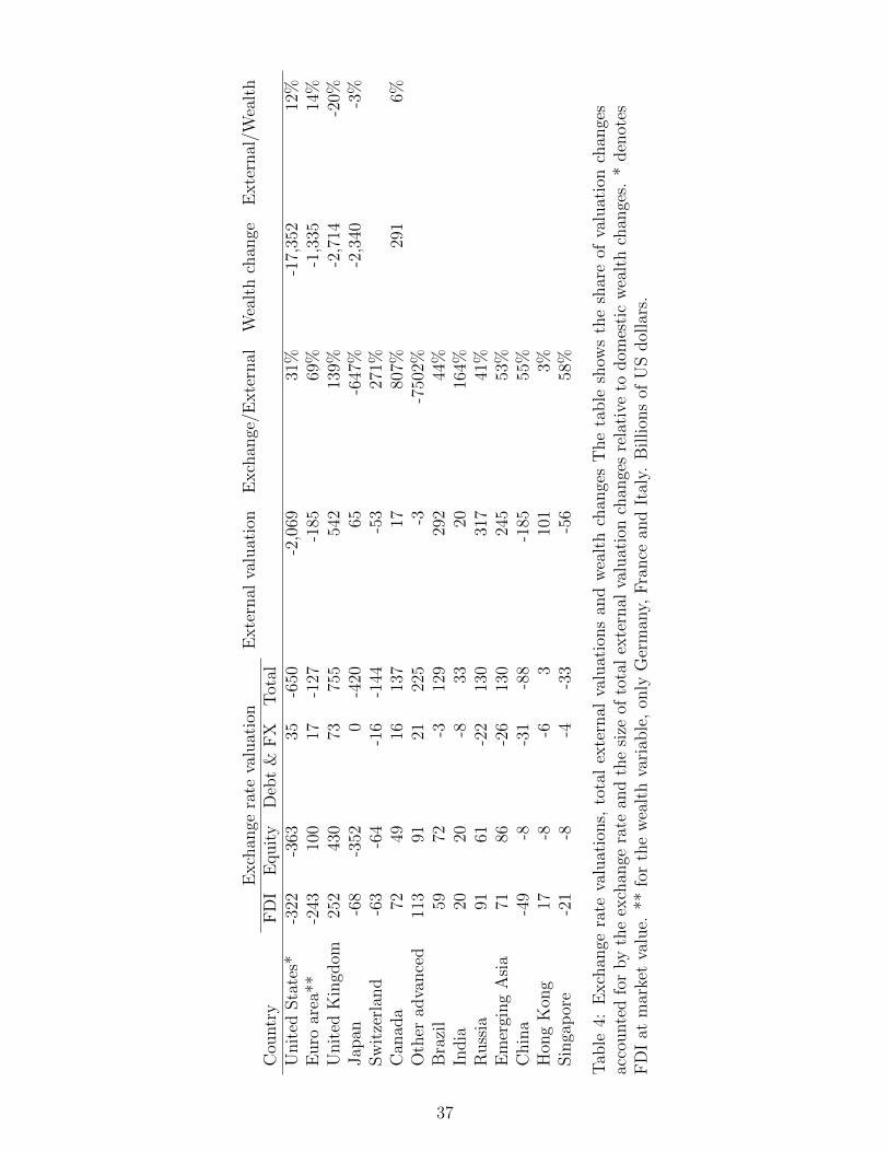
Exch

ange

rate

valu

atio

nE

xte

rnal

valu

atio

nE

xch

ange

/Exte

rnal

Wea

lth

chan

geE

xte

rnal

/Wea

lth

Cou

ntr

yF

DI

Equit

yD

ebt

&F

XT

otal

Unit

edSta

tes*

-322

-363

35-6

50-2

,069

31%

-17,

352

12%

Euro

area

**-2

4310

017

-127

-185

69%

-1,3

3514

%U

nit

edK

ingd

om25

243

073

755

542

139%

-2,7

14-2

0%Jap

an-6

8-3

520

-420

65-6

47%

-2,3

40-3

%Sw

itze

rlan

d-6

3-6

4-1

6-1

44-5

327

1%C

anad

a72

4916

137

1780

7%29

16%

Oth

erad

vance

d11

391

2122

5-3

-750

2%B

razi

l59

72-3

129

292

44%

India

2020

-833

2016

4%R

uss

ia91

61-2

213

031

741

%E

mer

ging

Asi

a71

86-2

613

024

553

%C

hin

a-4

9-8

-31

-88

-185

55%

Hon

gK

ong

17-8

-63

101

3%Sin

gap

ore

-21

-8-4

-33

-56

58%

Tab

le4:

Exch

ange

rate

valu

atio

ns,

tota

lex

tern

alva

luat

ions

and

wea

lth

chan

ges

The

table

show

sth

esh

are

ofva

luat

ion

chan

ges

acco

unte

dfo

rby

the

exch

ange

rate

and

the

size

ofto

tal

exte

rnal

valu

atio

nch

ange

sre

lati

veto

dom

esti

cw

ealt

hch

ange

s.*

den

otes

FD

Iat

mar

ket

valu

e.**

for

the

wea

lth

vari

able

,on

lyG

erm

any,

Fra

nce

and

Ital

y.B

illion

sof

US

dol

lars

.

37

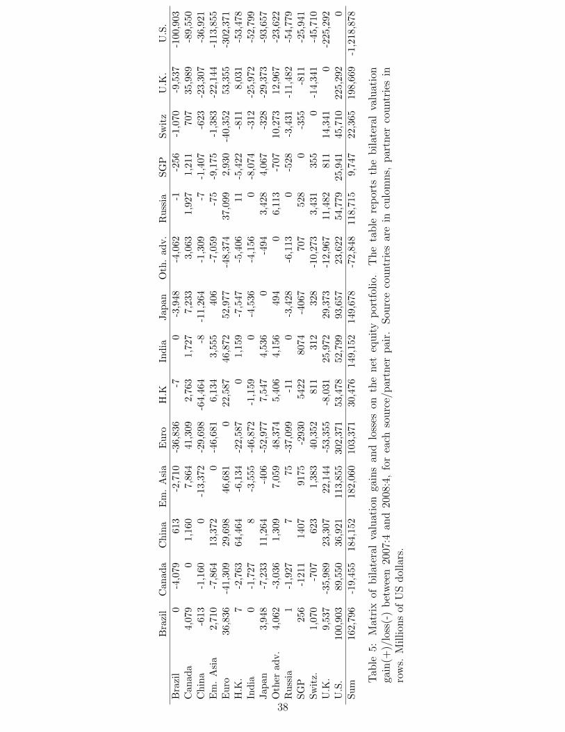
Bra

zil

Can

ada

Ch

ina

Em

.A

sia

Eu

roH

.KIn

dia

Jap

anO

th.

ad

v.

Ru

ssia

SG

PS

wit

zU

.K.

U.S

.

Bra

zil

0-4

,079

613

-2,7

10-3

6,83

6-7

0-3

,948

-4,0

62

-1-2

56

-1,0

70

-9,5

37

-100,9

03

Can

ada

4,07

90

1,16

07,

864

41,3

092,

763

1,72

77,

233

3,063

1,9

27

1,2

11

707

35,9

89

-89,5

50

Ch

ina

-613

-1,1

600

-13,

372

-29,

698

-64,

464

-8-1

1,26

4-1

,309

-7-1

,407

-623

-23,3

07

-36,9

21

Em

.A

sia

2,71

0-7

,864

13,3

720

-46,

681

6,13

43,

555

406

-7,0

59

-75

-9,1

75

-1,3

83

-22,1

44

-113,8

55

Eu

ro36

,836

-41,

309

29,6

9846

,681

022

,587

46,8

7252

,977

-48,3

74

37,0

99

2,9

30

-40,3

52

53,3

55

-302,3

71

H.K

.7

-2,7

6364

,464

-6,1

34-2

2,58

70

1,15

9-7

,547

-5,4

06

11

-5,4

22

-811

8,0

31

-53,4

78

Ind

ia0

-1,7

278

-3,5

55-4

6,87

2-1

,159

0-4

,536

-4,1

56

0-8

,074

-312

-25,9

72

-52,7

99

Jap

an3,

948

-7,2

3311

,264

-406

-52,

977

7,54

74,

536

0-4

94

3,4

28

4,0

67

-328

-29,3

73

-93,6

57

Oth

erad

v.

4,06

2-3

,036

1,30

97,

059

48,3

745,

406

4,15

649

40

6,1

13

-707

10,2

73

12,9

67

-23,6

22

Ru

ssia

1-1

,927

775

-37,

099

-11

0-3

,428

-6,1

13

0-5

28

-3,4

31

-11,4

82

-54,7

79

SG

P25

6-1

211

1407

9175

-293

054

2280

74-4

067

707

528

0-3

55

-811

-25,9

41

Sw

itz.

1,07

0-7

0762

31,

383

40,3

5281

131

232

8-1

0,273

3,4

31

355

0-1

4,3

41

-45,7

10

U.K

.9,

537

-35,

989

23,3

0722

,144

-53,

355

-8,0

3125

,972

29,3

73-1

2,967

11,4

82

811

14,3

41

0-2

25,2

92

U.S

.10

0,90

389

,550

36,9

2111

3,85

530

2,37

153

,478

52,7

9993

,657

23,6

22

54,7

79

25,9

41

45,7

10

225,2

92

0

Su

m16

2,79

6-1

9,45

518

4,15

218

2,06

010

3,37

130

,476

149,

152

149,

678

-72,

848

118,7

15

9,7

47

22,3

65

198,6

69

-1,2

18,8

78

Tab

le5:

Mat

rix

ofbilat

eral

valu

atio

nga

ins

and

loss

eson

the

net

equit

yp

ortf

olio

.T

he

table

rep

orts

the

bilat

eral

valu

atio

nga

in(+

)/lo

ss(-

)b

etw

een

2007

:4an

d20

08:4

,fo

rea

chso

urc

e/par

tner

pai

r.Sou

rce

countr

ies

are

incu

lom

ns,

par

tner

countr

ies

inro

ws.

Million

sof

US

dol

lars

.

38

Bra

zil

Can

ada

Chin

aE

m.

Asi

aE

uro

H.K

.Jap

anO

ther

adv.

Russ

iaSG

PSw

itz.

U.K

.U

.S.

Bra

zil

0-3

220

2,29

3-7

,961

43,

502

-1,0

89-2

-14

195

-2,6

823,

367

Can

ada

322

0-2

160

2,35

2-1

09-3

,998

2,49

336

-96

1,10

71,

224

2,34

2C

hin

a0

20

-15

7,43

63,

298

-2,7

12-4

85

644

134

5-1

5,44

5E

m.

Asi

a-2

,293

-160

150

-23,

596

-3,1

352,

637

2,69

4-2

8-1

8,13

430

3-4

,892

6,78

7E

uro

7,96

1-2

,352

-7,4

3623

,596

0-9

,263

-78,

117

1,80

35,

793

-6,8

51-7

,479

29,2

4458

,566

H.K

.-4

109

-3,2

983,

135

9,26

30

-13,

138

7,67

8-8

673

336

0-1

6,61

8-3

,044

Jap

an-3

,502

3,99

82,

712

-2,6

3778

,117

13,1

380

-14,

909

300

812

-1,8

28-8

,095

15,9

30O

ther

adv.

1,08

9-2

,493

48-2

,694

-1,8

03-7

,678

14,9

090

735

-5,6

19-1

,904

-17,

100

2,34

7R

uss

ia2

-36

-528

-5,7

9386

-300

-735

0-9

3-6

4-7

,411

-2,3

53SG

P14

96-6

4418

,134

6,85

1-7

33-8

125,

619

930

271,

787

2,35

5Sw

itz.

-195

-1,1

07-1

-303

7,47

9-3

601,

828

1,90

464

-27

09,

691

3,59

8U

.K.

2,68

2-1

,224

-345

4,89

2-2

9,24

416

,618

8,09

517

,100

7,41

1-1

,787

-9,6

910

-132

,915

U.S

.-3

,367

-2,3

4215

,445

-6,7

87-5

8,56

63,

044

-15,

930

-2,3

472,

353

-2,3

55-3

,598

132,

915

0Sum

2,70

9-5

,829

6,48

939

,802

-15,

464

14,9

10-8

4,03

820

,163

16,6

73-3

2,78

6-2

2,57

311

8,40

9-5

8,46

4

Tab

le6:

Mat

rix

ofbilat

eral

valu

atio

nga

ins

and

loss

eson

the

net

deb

tp

ortf

olio

.T

he

table

rep

orts

the

bilat

eral

valu

atio

nga

in(+

)/lo

ss(-

)b

etw

een

2007

:4an

d20

08:4

,fo

rea

chso

urc

e/par

tner

pai

r.Sou

rce

countr

ies

are

incu

lom

ns,

par

tner

countr

ies

inro

ws.

Million

sof

US

dol

lars

.

39

Bra

zil

Can

ada

Ch

ina

Em

.A

sia

Eu

roH

.K.

Ind

iaJap

anO

th.

ad

v.

Ru

ssia

SG

PS

wit

z.U

.K.

U.S

.

Bra

zil

010

,200

-339

n.a

.n

.a.

n.a

.n.a

.-5

,876

-4,2

87

na

n.a

.-6

,426

-3,6

23

-44,3

98

Can

ada

-10,

200

077

92,

524

-12,

770

2,46

08,

075

-10,

354

5,723

547

1,9

87

-7,5

19

-14,0

77

-70,1

57

Ch

ina

339

-779

0-3

,236

3,12

5-8

5,81

6-2

9-2

8,20

2-2

,139

1,7

43

8,8

19

-1,3

50

-2,3

53

-4,0

89

Em

.A

sia

n.a

.-2

,524

3,23

60

n.a

.-3

16n

.a.

-56,

466

-6,4

53

n.a

.8,7

03

-6,4

52

-18,5

15

-47,7

48

Eu

ron

.a.

12,7

70-3

,125

n.a

.0

n.a

.n

.a.

-143

,819

25,2

93

n.a

.7,3

48

-62,0

18

-96,8

31

-315,2

57

H.K

.n

.a.

-2,4

6085

,816

316

n.a

.0

n.a

.-6

,970

-2,3

06

n.a

.1,4

76

-1,8

87

-52,6

41

-37,3

07

Ind

ian

.a.

-8,0

7529

n.a

.n

.a.

n.a

.0

1,19

7-4

28

n.a

.4,5

22

-1,1

01

-5,5

75

-9,5

30

Jap

an5,

876

10,3

5428

,202

56,4

6614

3,81

96,

970

-1,1

970

22,3

11

117

18,5

26

-3,8

86

34,7

18

69,0

84

Oth

erad

v.

4,28

7-5

,723

2,13

96,

453

-25,

293

2,30

642

8-2

2,31

10

2,3

95

369

-3,2

47

-30,1

25

2,7

88

Ru

ssia

n.a

.-5

47-1

,743

n.a

.n

.a.

n.a

.n

.a.

-117

-2,3

95

0n

.a.

-2,1

48

-13,0

27

-7,7

39

SG

Pn

.a.

-1,9

87-8

,819

-8,7

03-7

,348

-1,4

76-4

,522

-18,

526

-369

n.a

.0

-7,6

24

-5,4

03

-90,1

58

Sw

itz.

6,42

67,

519

1,35

06,

452

62,0

181,

887

1,10

13,

886

3,427

2,1

48

7,6

24

0-2

,869

-9,0

19

U.K

.6,

323

14,0

772,

353

18,5

1596

,831

52,6

415,

575

-34,

718

30,1

25

13,0

27

5,4

03

2,8

69

025,3

55

U.S

.44

,398

70,1

574,

089

47,7

4831

5,25

737

,307

9,53

0-6

9,08

4-2

,788

7,7

39

90,1

58

9,0

19

-25,3

55

0

Su

m54

,749

102,

981

113,

969

126,

535

575,

639

15,9

6318

,962

-391

,361

65,5

34

27,7

16

154,9

35

-91,7

70

-235,6

77

-538,1

75

Tab

le7:

Mat

rix

ofbilat

eral

valu

atio

nga

ins

and

loss

eson

the

net

FD

Ip

ortf

olio

.T

he

table

rep

orts

the

bilat

eral

valu

atio

nga

in(+

)/lo

ss(-

)b

etw

een

2007

:4an

d20

08:4

,fo

rea

chso

urc

e/par

tner

pai

r.Sou

rce

countr

ies

are

incu

lom

ns,

par

tner

countr

ies

inro

ws.

Sou

rce/

par

tner

pai

rsw

ith

bilat

eral

dir

ect

inve

stm

ent

pos

itio

ns

unav

aila

ble

atm

arke

tva

lue

are

den

oted

wit

hn.a

..M

illion

sof

US

dol

lars

.

40

Bra

zil

Can

ada

Chin

aE

m.

Asi

aE

uro

H.K

.In

dia

Jap

anO

ther

adv.

Russ

iaSG

PSw

itz.

U.K

.U

.S.

Bra

zil

00

00

00

00

00

00

00

Can

ada

00

00

00

00

00

00

00

Chin

a0

00

00

00

00

00

00

0E

m.

Asi

a0

00

00

00

00

00

00

0E

uro

-501

-256

-5,3

92-1

,581

0-2

07-1

,036

-2,2

58-1

,134

-2,6

82-5

71-2

83-3

91-2

84H

.K.

00

00

00

00

00

00

00

India

00

00

00

00

00

00

00

Jap

an0

948,

166

4,45

184

554

485

20

1,35

366

42,

294

791

783

4,42

6O

ther

adv.

00

00

00

00

00

00

00

Russ

ia0

00

00

00

00

00

00

0SG

P0

00

00

00

00

00

00

0Sw

itz.

00

075

172

913

00

037

00

0U

.K.

00

-12,

626

-8,6

82-5

,982

-721

-2,6

150

-855

-7,5

48-1

,926

-734

00

U.S

.1,

786

241

12,4

721,

662

1,80

51,

531

2,07

69,

802

733

2,75

11,

122

156

186

0Sum

1,28

471

2,62

04,

075

-3,1

601,

156

-710

7,54

497

-6,8

1595

6-7

057

74,

143

Tab

le8:

Mat

rix

ofbilat

eral

valu

atio

nga

ins

and

loss

eson

the

fore

ign

exch

ange

rese

rves

.T

he

table

rep

orts

the

bilat

eral

valu

atio

nga

in(+

)/lo

ss(-

)b

etw

een

2007

:4an

d20

08:4

,fo

rea

chso

urc

e/par

tner

pai

r.Sou

rce

countr

ies

are

incu

lom

ns,

par

tner

countr

ies

inro

ws.

Million

sof

SD

R.

41

Appendix

A Countries and regional groups

Individual countries:Brazil, Canada, China, Hong Kong, India, Japan, Russia, Singapore, Switzerland, UnitedKingdom, United States

Regional groups:Emerging Asia: Indonesia, Korea, Malaysia, Philippines, Thailand.Euro area: Austria, Belgium, Finland, France, Germany, Greece, Ireland, Italy, Luxembourg,Netherlands, Portugal, Slovenia, Spain.Other advanced countries: Australia, Denmark, New Zealand, Norway, Sweden.

Country groups that are only included as a vis-a-vis category:Offshore centers: Aruba, Andorra, Bahamas, Barbados, Bermuda, British Virgin Islands,Cayman Islands, Gibraltar, Guernsey, Isle of Man, Jersey, Lebanon, Liechtenstein, Macao,Mauritius, Monaco, Netherlands Antilles, Panama, Samoa, San Marino, Vanuatu, Vatican,West Indies.Oil exporters: Algeria, Bahrain, Gabon, Iran, Iraq, Kuwait, Libya, Nigeria, Oman, Qatar,Saudi Arabia, United Arab Emirates.Other Latin American countries: Argentina, Chile, Mexico.

B Data Appendix

B.1 Aggregate positions and flows

International Investment Position (except foreign exchange reserves): we rely on na-tional sources for Canada (Statistics Canada), China (State Administration of Foreign Ex-change (SAFE)), Euro Area (European Central Bank), Japan (Bank of Japan), Switzerland(Swiss National Bank), United Kingdom (Pink Book) and the United States (Bureau ofEconomic Analysis). Data for all other countries were obtained from the IMF Balance ofPayments database.

Foreign exchange reserves: we use “total reserves minus gold” available from the IMFInternational Financial Statistics database.

Financial flows: IMF Balance of Payments statistics

B.2 Bilateral positions

The data construction closely follows Milesi-Ferretti, Strobbe and Tamirisa (2010). Wecollect annual bilateral positions data for end-2007 and end-2008.

Brazil

42

FDI: reported bilateral FDI assets and liabilities are measured at book value. To obtainmarket value estimates of Brazil’s bilateral direct investment positions, we use market valuedata derived from partner countries’ reported assets and liabilities vis-a-vis Brazil. Bilateralpositions are imputed from the following countries: Australia, Canada, China, Denmark,Japan, New Zealand, Norway, Sweden, Switzerland, United Kingdom and the United States.Portfolio equity and debt: based on reported and derived portfolio equity/debt assetsand liabilities available in IMF Coordinated Portfolio Investment Survey tables 1.1, 1.2 and5.1, 5.2.Foreign Exchange Reserves: following Milesi-Ferretti et al. (2010), the US dollar shareof total reserves is estimated as the difference between US debt liabilities vis-a-vis Brazil andBrazil’s debt assets in the US as reported in the CPIS. The remainder is assumed to be heldin euros.

Canada

FDI: we use the data on Canadian direct investment abroad and foreign direct investmentto Canada by country and sector available from the Office of the Chief Economist of the Cana-dian Ministry of Foreign Affairs and International Trade (http://www.international.gc.ca/economist-economiste/statistics-statistiques/investments-investissements.aspx?lang=eng)Portfolio equity and debt: based on reported and derived portfolio equity/debt assetsand liabilities available in IMF Coordinated Portfolio Investment Survey tables 1.1, 1.2 and5.1, 5.2.Foreign exchange reserves: we use the currency composition of reserves published by theCanadian department of Finance (http://www.fin.gc.ca/pub/oir-ro-archives-eng.asp)

China

China does not report the geographical allocation of its portfolio investment holdings,as it does not take part in the CPIS. We investigated details national sources and handcollected data to remedy this shortcoming. International Investment Position data are notat market value in official sources (SAFE). We construct data on bilateral equity assets andliability and market value as well as data on debt assets. We also manage to reconstructbilateral FDI assets and liabilities at market value using Ministry of Commerce data. Wereconstructed bilateral data on Chinese external assets at market value from various Chinesedata sources.

FDI Assets: The only market value estimates of Chinese FDI have been done in 2004.Thiswas the first survey ever been done on Chinese FDI. After 2004, government agencies addedup flow data to estimate the official IIP. Therefore, the official IIP of 2005-2011 are not atmarket value.We obtain Ministry of Commerce data with a very good geographical breakdown. Theaggregate numbers are not exactly identical to the IIP SAFE numbers as the Ministry ofCommerce has a different statistics standard from SAFE. The data are at market value sowe use the 2004 stock (based on survey data) and cumulate flows using the correspondingstock indexes for valuation adjustment.FDI Liabilities: We use the 2004 stock (based on survey data) and cumulate flows usingthe Shanghai stock index for valuation adjustment.

43

Portfolio debt: Portfolio debt is held mainly by 5 Chinese state-owned international banks(Bank of China, Industrial and Commercial Bank of China, China Construction Bank, Agri-cultural Bank of China, Chinese Development Bank) and the sovereign wealth fund CIC. Wehave a detailed geographical decomposition of cross border claims (into Hong Kong, OtherAsia Pacific locations, North and South America, Europe, Middle East and Africa) , andseparately, a currency breakdown (RMB, dollar, euro, HK dollar, yen, CHF and other) ofoverseas loans and of securities held for the Bank of China33. In 2010, the total amountof cross border claims for BoC is 1,260,10 millions RMB while the amount of non RMBassets is about double at 2,526,5777 millions RMB. This indicates that a sizable amountof the domestic assets of the BoC are in foreign currency. Making a set of straightforwardassumptions34, we are able to construct for 2007-2010 a table of cross border security hold-ings disaggregated by country and currency. The Bank of China is historically the mainplayer overseas (Bank of China has been ranked No. 3 in 2009 within all banks in the worldby market capitalization). We have a coarser set of data for the three other banks (ICC,CCB, ABC). We obtained as detailed data as possible from the banks report. For the otherbanks (except CDB), we could obtain data only on their cross border claims by locations.We apply the Bank of China weights to allocate assets between investment securities andtotal claims, by location, thereby constructing a table of securities by location35. For CDB,we obtained securities by currencies. We allocated the dollar securities to the US and the(small) remainder of overseas currency securities to Hong Kong.

33We have a breakdown into: derivative financial assets; loans and advances to customers (net); investmentsecurities (broken down in available for sale ; held to maturity and loans and receivables) and other assets.We present in our spreadsheet all the source data we gathered. We work with the assumptions that all theinvestment securities are debt securities. In principle they could also be equities. In 2007-2008 however wehave the exact amount of portfolio equity bought by all our 5 banks via the QDII system (see below forthe construction of portfolio equity assets). This amount is less than $4 bn, so we treat it as negligible (theorder of magnitude of our total debt asset numbers are in the range of $200 bn).

34The data indicate that there is more Hong Kong dollar assets than claims to Hong Kong, more dollarassets than claims to North and South America, less euro and sterling assets than claims to Europe, lessyen assets than claims to other Asia Pacific location. We make the following assumptions: all Hong Kongclaims are in HK$; all euro and sterling assets are to Europe, all yen assets are to ”other Asia Pacific”; allNorth and South America, Middle East and Africa claims are in $. Any remaining Europe claims not ineuro or sterling are assumed to be in $, any other Asia Pacific claims not in yen are assumed to be in US $.We compute the share of investment securities in total US $ assets and use this weight to derive securitiesholdings in dollar portfolios, for all geographical areas.

We focus on the investment securities part of the claims (securities available for sale; held to maturity andloans and receivables) of the bank balance sheet. We do not use here the data on loans. We check that thetotal amount of US $ securities we obtain for cross border holdings is inferior to the total amount of reportedUS $ securities in the total assets of the bank. For example for 2010, the amount of US $ denominatedcross border securities we estimate is 105, 883 millions RMB and the reported US dollars securities of thebank amount to 290,943 millions RMB. The difference is therefore domestic holdings of US $ denominatedsecurities.

35We give below the market capitalization of the four largest stated owned banks in China.The Bank ofChina (BoC), the Industrial and Commercial Bank of China (ICBC), the China Construction Bank (CCB), the Agricultural Bank of China (ABC). These are the only banks having significant international activityand its is clear that the Bank of China is by far the most international one.

Banks: (2010) Bank of China ICBC CCB ABCTotal Assets (million RMB) 10,459,865 12,779,711 10,810,317 10,337,406Cross border claims (million RMB) 1,260,170 381,982 272,829 82,254overseas assset ratio 12.0% 3.9% 2.5% 0.8%

44

We have data on fixed income holdings for CIC but we do not have explicit geographicaldata. We are told however (private communication with Chinese sources) that it is almostall US debt.It is our belief that the union of these five banks and CIC cover the universe of Chineseinvestors in international debt assets (foreign exchange reserves are accounted for separetely).Portfolio debt liabilities: We do not have any direct source for debt liabilities and haveto take the official IIP numbers. The amount involved are very small (in the order of 20times smaller than debt assets according to the IIP data).Foreign exchange reserves: The currency composition of the Chinese reserves is notdisclosed. Nevertheless, we have one snapshot of the currency weights. In September 2010,the China Securities Journal revealed the following breakdown for the $2,450 billion reservesof the People’s Bank of China: 65% in dollars, 26% in euros, 5% in sterling, and 3% in yen.We assume that these weights are similar in 2007-2008, as they are likely to be slow moving(by doing so we probably slightly underestimate the dollar share in 2007-2008). For theaggregate amount of reserves we use total reserves minus gold from IFS.Portfolio equity assets: Equity investment overseas is strictly regulated. QDII is a quotasystem for domestic investors to hold equity abroad. We obtained a record of all authorizedinvestments in foreign equity for the years 2006-2010. from SAFE. According to Chinesesources, most of the investment reported in QDII is in equity, ETFs or commodities. Un-fortunately, we have the breakdown by domestic investor name but not disaggregated bygeographical area of investment. However, the amounts involved are very small due to QDIIhaving been launched only in 2006. Besides, China does not have many wealth managementservices to help Chinese invest in overseas equity markets. For 2006, the total flows amountto $9,675 million, for 2007 $30,544.7 million and for 2008 $3,255 million. Furthermore, pri-vate communication with Chinese sources indicate that about 50% of the QDII allocation isequity out of which about 40% is in the Hong Kong market 5% to the US and 5% to Sin-gapore. We value the remaining QDII assets using a global commodity price index (SourceIMF: PALLFNF Index).We have detailed data on the geographical location of the equity holdings of the sovereignwealth fund CIC. It is our belief that CIC and QDII cover the entire spectrum of portfolioequity investment overseas.Portfolio equity liabilities: We use partner country data.

Emerging Asia

FDI: reported bilateral FDI assets and liabilities are measured at book value. To obtainmarket value estimates of Emerging Asia’s bilateral direct investment positions, we usemarket value data derived from partner countries’ reported assets and liabilities vis-a-visEmerging Asia. Bilateral positions are imputed from the following countries: Australia,Canada, China, Denmark, Hong Kong, Japan, New Zealand, Norway, Singapore, Sweden,Switzerland, United Kingdom and the United States.Portfolio equity and debt: based on reported and derived portfolio equity/debt assetsand liabilities available in IMF Coordinated Portfolio Investment Survey tables 1.1, 1.2 and5.1, 5.2.Foreign exchange reserves: We use the 2007 currency composition in Milesi-Ferretti,Strobbe and Tamirisa (2010), netting-out the Taiwan-US debt liabilities position from the

45

Milesi-Ferretti, Strobbe and Tamirisa (2010) bilateral USD FX position. For 2008, we assumethat the currency share is unchanged from 2007.

Euro Area

FDI: reported bilateral FDI assets and liabilities are measured at book value. To obtainmarket value estimates of the Euro area’s bilateral direct investment positions, we use marketvalue data derived from partner countries’ reported assets and liabilities vis-a-vis the Euroarea. Bilateral positions are imputed from the following countries: Australia, Canada, China,Denmark, Japan, New Zealand, Norway, Singapore, Sweden, Switzerland, United Kingdomand the United States. The Euro area total is calculated as the sum of the individual membercountries bilateral positions.Portfolio equity and debt: based on reported and derived portfolio equity/debt assetsand liabilities available in IMF Coordinated Portfolio Investment Survey tables 1.1, 1.2 and5.1, 5.2. The Euro are total is calculated as the sum of the individual member countriesbilateral positions, netting-out the intra Euro area positions.Foreign exchange reserves: we use the 2007 currency composition in Milesi-Ferretti,Strobbe and Tamirisa (2010) and, for 2008, assume that the currency shares are unchangedfrom 2007.

Hong Kong

FDI: we use tables 050 and 048 on the geographical breakdown of outward and inward FDIpublished by the Census and Statistics Department of the Government of Hong Kong.(http://www.censtatd.gov.hk/hong kong statistics/statistics by subject/index.jsp)Portfolio equity and debt: based on reported and derived portfolio equity/debt assetsand liabilities available in IMF Coordinated Portfolio Investment Survey tables 1.1, 1.2 and5.1, 5.2.Foreign exchange reserves: we use the 2007 currency composition in Milesi-Ferretti,Strobbe and Tamirisa (2010) and, for 2008, assume that the currency shares are unchangedfrom 2007.

India

FDI: reported bilateral FDI assets and liabilities are measured at book value. To obtainmarket value estimates of India’s bilateral direct investment positions, we use market valuedata derived from partner countries’ reported assets and liabilities vis-a-vis India. Bilateralpositions are imputed from the following countries: Australia, Canada, China, Denmark,Japan, New Zealand, Norway, Singapore, Sweden, Switzerland, United Kingdom and theUnited States.Portfolio equity and debt: based on reported and derived portfolio equity/debt assetsand liabilities available in IMF Coordinated Portfolio Investment Survey tables 1.1, 1.2 and5.1, 5.2.Foreign exchange reserves: we estimate the currency composition of reserves based onthe aggregate currency shares for emerging markets in the IMF COFER database.

Japan

46

FDI: we use the geographical breakdown of outward and inward FDI provided in the Bank ofJapan publication “Regional direct investment position assets and liabilities (end of 2009)”(http://www.boj.or.jp/en/statistics/br/bop/index.htm/)Portfolio equity and debt: based on reported and derived portfolio equity/debt assetsand liabilities available in IMF Coordinated Portfolio Investment Survey tables 1.1, 1.2 and5.1, 5.2.Foreign exchange reserves: we use the 2007 currency composition in Milesi-Ferretti,Strobbe and Tamirisa (2010) and, for 2008, assume that the currency shares are unchangedfrom 2007.

Other advanced

FDI: For Australia we use table 2, “Foreign Investment in Australia, Level of Investment bycountry and Country Groups by type of investment and year”, and table 5 “Australian Invest-ment Abroad, Level of Investment by country and Country Groups by type of investment andyear” provided by the Australian Bureau of Statistics (http://www.abs.gov.au/AUSSTATS).For Denmark we use the geographical breakdown provided in table 3 “Direct Investments bro-ken down by country” provided by the central bank of Denmark ( http://www.nationalbanken.dk).For New Zealand we use the geographical breakdown provided in table 3: ”Stock of directinvestment by country” in the “Balance of Payments and International Investment Position:Year ended 31 March 2010” provided by Statistics New Zealand (http://www.stats.govt.nz).For Sweden and Norway we obtain the geographical breakdown of direct investment from theOECD (http://stats.oecd.org/BrandedView.aspx?oecd bv id=idi-data-en&doi=data-00337-en).Portfolio equity and debt: based on reported and derived portfolio equity/debt assetsand liabilities available in IMF Coordinated Portfolio Investment Survey tables 1.1, 1.2 and5.1, 5.2. The country group total is calculated as the sum of the individual member countriesbilateral positions.Foreign exchange reserves: we use the 2007 currency composition in Milesi-Ferretti,Strobbe and Tamirisa (2010) and assume that the 2008 currency shares are unchanged from2007.

Russia

FDI: reported bilateral FDI assets and liabilities are measured at book value. To obtainmarket value estimates of Russia’s bilateral direct investment positions, we use market valuedata derived from partner countries’ reported assets and liabilities vis-a-vis Russia. Bilateralpositions are imputed from the following countries: Australia, Canada, China, Denmark,Japan, New Zealand, Norway, Sweden, Switzerland, United Kingdom and the United States.Portfolio equity and debt: based on reported and derived portfolio equity/debt assetsand liabilities available in IMF Coordinated Portfolio Investment Survey tables 1.1, 1.2 and5.1, 5.2.Foreign exchange reserves: we use the currency composition reported in the annualreports of the central bank of Russia (http://www.cbr.ru/eng/publ/main.asp?Prtid=God).

Singapore

47

FDI: for outward direct investment we use table 2 “Total Direct Investment Abroad by Coun-try/Region, 2000-2009” of the report “Singapore’s Investment Abroad 2009” and for inwarddirect investment we use table 2 “Foreign Direct Investment in Singapore by Country/Region,1998-2008” of the report “Foreign equity investment in Singapore, 2008”. Both reports arepublished by Statistics Singapore (http://www.singstat.gov.sg/pubn/business.html).Portfolio equity and debt: based on reported and derived portfolio equity/debt assetsand liabilities available in IMF Coordinated Portfolio Investment Survey tables 1.1, 1.2 and5.1, 5.2.Foreign exchange reserves: we use the 2007 currency composition in Milesi-Ferretti,Strobbe and Tamirisa (2010) and assume that the 2008 currency shares are unchanged from2007.

Switzerland

FDI: we rely on the geographical composition provided in table 1.2 “Swiss direct investmentabroad by country” (http://www.snb.ch/en/iabout/stat/statpub/fdi/stats/fdi/fdi ChDirAus LgKapBe)and table 2.2 “Foreign direct investment in Switzerland, by country”(http://www.snb.ch/en/iabout/stat/statpub/fdi/stats/fdi/fdi AusDirCh KapBeHL) publishedby the Swiss National Bank.Portfolio equity and debt: based on reported and derived portfolio equity/debt assetsand liabilities available in IMF Coordinated Portfolio Investment Survey tables 1.1, 1.2 and5.1, 5.2.Foreign exchange reserves: we use the currency allocation of official reserves provided inchapter 5 of the annual reports of the Swiss National Bank(http://www.snb.ch/en/iabout/pub/annrep/id/pub annrep)

United Kingdom

FDI: we use the geographical composition provided in table 3.1 “Net FDI international in-vestment position abroad analysed by area and main country, end 2000 to end 2009” andtable 6.1 “Net FDI International positions in the United Kingdom analysed by area and maincountry, 2000 to 2009” in the “Foreign Direct Investment Business Monitor MA4” publishedby the Office of National Statistics (http://www.statistics.gov.uk/statbase/product.asp?vlnk=9614).Portfolio equity and debt: based on reported and derived portfolio equity/debt assetsand liabilities available in IMF Coordinated Portfolio Investment Survey tables 1.1, 1.2 and5.1, 5.2.Foreign exchange reserves: we use the currency composition of the UK government’s of-ficial reserves published in the quarterly annex to the “UK International Reserves & ForeignCurrency Liquidity Template” (http://www.bankofengland.co.uk/statistics/reserves/intro.htm).

United States

FDI: for bilateral outward direct investment we rely on the table “U.S. direct InvestmentAbroad: Selected Items by Detailed Country, 2005-2009”(http://www.bea.gov/international/di1usdbal.htm) and for bilateral inward direct invest-ment on the table “Foreign Direct Investment in the United States: Selected Items by De-tailed Country, 2005-2009” (http://www.bea.gov/international/xls/LongCountry.xls) bothpublished by the Bureau of Economic Analysis.

48

Portfolio equity and debt: for portfolio equity and debt assets we use IMF CPIS tables1.1 and 1.2. Portfolio equity and debt liabilities were obtained from the Survey on PortfolioHoldings of U.S. Securities as of June 2007 and June 2008, published by the U.S. Treasury (HREFhttp://www.treasury.gov/resource-center/data-chart-center/tic/Pages/fpis.aspx). Po-sitions are updated using the monthly estimates provided in Bertaut and Tryon (2007)(HREFhttp://www.federalreserve.gov/pubs/ifdp/2007/910/default.htm)Foreign exchange reserves: we use the 2007 currency composition in Milesi-Ferretti,Strobbe and Tamirisa (2010) and assume that the 2008 currency shares are unchanged from2007.

B.3 FDI market value estimation

We denote market value by MV, book value by BV, current cost by CC and historical costby HV. The list of countries providing both aggregate and bilateral FDI positions data atMV includes:

• Australia (IIP & bilateral positions; see http://abs.gov.au/austats/abs@.nsf/mf/5370.0.55.001)

• Hong Kong (IIP & bilateral positions)

• New Zealand (IIP & bilateral positions, except for some firms that provide positionsat BV; see http://www.unctad.org/sections/dite fdistat/docs/wid cp nz en.pdf)

• Norway (IIP & bilateral positions; see http://www.ssb.no/intinvpos en/about.html)

For the following countries, we estimate both the aggregate FDI positions and the bilateralpositions at MV:

• Canada (IIP & bilateral positions = BV, we estimate MV, initial 2005 market to bookvalue ratio provided by Simard and Boulay (n.d.))

• China (IIP & bilateral positions = BV, we estimate MV, initial 2004 aggregate andbilateral FDI positions are at market value)

• Denmark (IIP & bilateral positions = BV, we estimate MV, initial 2006 market valueestimate provided by Kumah, Damgaard and Elkjaer (2009))

• Switzerland (IIP & bilateral positions = BV, we estimate MV, initial 2005 marketvalue estimate provided by Stoffes and Tille (2009))

• United Kingdom (IIP & bilateral positions = BV, we estimate MV, initial 2005 marketvalue estimate provided by Kubelec, Orskaug and Tanaka (2007))

Countries providing aggregate FDI data at market value along with official valuation series:

• Japan (IIP & bilateral positions = BV, Bank of Japan provides estimate of aggre-gate FDI abroad & inward market-to-book value ratio, we use this to obtain bilateralpositions at MV)

49

• Sweden (IIP & bilateral positions = BV, also provides estimate of aggregate FDI atMV, we use these to obtain bilateral positions at MV)

• United States (IIP = CC, BEA bilateral positions = HC, market-to-HC ratio providedby BEA, we use these to obtain bilateral positions at MV)

The following countries do not report aggregate FDI at MV and we are unable to computeour own estimates. Reported bilateral positions are at BV.

• Brazil (IIP = BV, bilateral positions at MV imputed from partner countries)

• Emerging Asia (IIP = BV, bilateral positions at MV imputed from partner countries)

• Euro Area (IIP & bilateral = BV, bilateral positions at MV imputed from partnercountries)

• India (IIP = BV, bilateral positions at MV imputed from partner countries)

• Russia (IIP = BV, bilateral positions at MV imputed from partner countries)

Methodology for market value estimation:

1. we start from an initial estimate of the aggregate FDI abroad/inward position at MV(usually for 2005, provided by statistical agency or other, see above).

2. multiply the date t position in USD with the weighted average of the destinationcountries’ USD ex-dividend equity index returns, with weights corresponding to thedate t FDI portfolio weights (FDI abroad); or home country USD equity index return(inward FDI)

3. add USD financial outflow/inflow to obtain date t+1 position at MV

4. calculate market-to-book value ratio for each date

5. calculate bilateral positions at MV using 4)

Due to data limitations, we are unfortunately unable to obtain full bilateral FDI balancesheets at market value for those countries where positions were imputed from partner countryFDI assets and liabilities. Instances with bilateral positions unavailable for at least onecountry of a source/partner country pair are indicated with ”na” in the matrix of bilateralvaluation gains and losses on the net FDI portfolio.

50

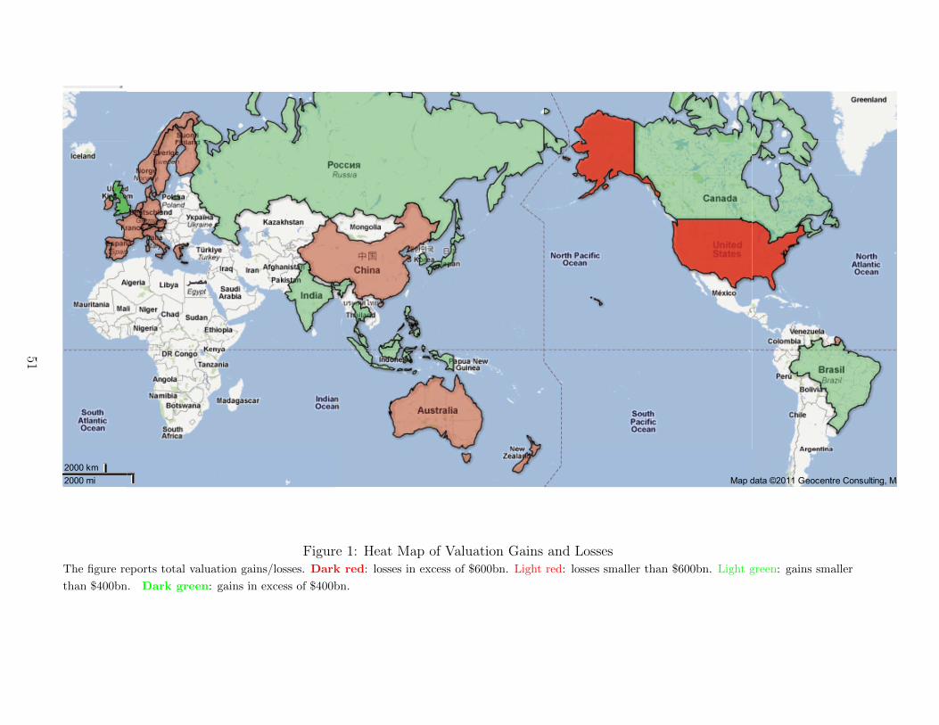
File View Edit Visualize Merge

Showing all rows options Map style saved.

Location kml_4326 Display as heat map Configure info window Configure styles Export to KML Get KML network link Get embeddable link

heatmap_082111 Natural Earth

2000 km

2000 mi Map data ©2011 Geocentre Consulting, MapLink, Tele Atlas

+Pierre-Olivier Gmail Calendar Documents Photos Reader Web more Pierre-Olivier Gourinchas 0 Share!

Figure 1: Heat Map of Valuation Gains and LossesThe figure reports total valuation gains/losses. Dark red: losses in excess of $600bn. Light red: losses smaller than $600bn. Light green: gains smaller

than $400bn. Dark green: gains in excess of $400bn.

51

Figure 2: Heat Map of Valuation Gains and LossesFile View Edit Visualize Merge

Showing all rows options Map style saved.

Location kml_4326 Display as heat map Configure info window Configure styles Export to KML Get KML network link Get embeddable link

heatmap_082111 Natural Earth

2000 km

2000 mi Map data ©2011 Geocentre Consulting, MapLink, Tele Atlas

+Pierre-Olivier Gmail Calendar Documents Photos Reader Web more Pierre-Olivier Gourinchas 0 Share!

(a) Portfolio Equity

File View Edit Visualize Merge

Showing all rows options Map style saved.

Location kml_4326 Display as heat map Configure info window Configure styles Export to KML Get KML network link Get embeddable link

heatmap_082111 Natural Earth

2000 km

2000 mi Map data ©2011 Geocentre Consulting, MapLink, Tele Atlas

+Pierre-Olivier Gmail Calendar Documents Photos Reader Web more Pierre-Olivier Gourinchas 0 Share!

(b) Portfolio Debt

The figure reports portfolio gains/losses for equity (panel (a)) and debt (panel(b)). Dark red: losses in

excess of $600bn. Light red: losses smaller than $600bn. Light green: gains smaller than $400bn. Dark

green: gains in excess of $400bn.

52

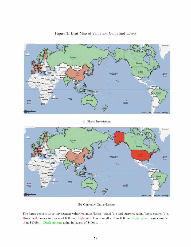
Figure 3: Heat Map of Valuation Gains and LossesFile View Edit Visualize Merge

Showing all rows options Map style saved.

Location kml_4326 Display as heat map Configure info window Configure styles Export to KML Get KML network link Get embeddable link

heatmap_082111 Natural Earth

2000 km

2000 mi Map data ©2011 Geocentre Consulting, MapLink, Tele Atlas

+Pierre-Olivier Gmail Calendar Documents Photos Reader Web more Pierre-Olivier Gourinchas 0 Share!

(a) Direct Investment

File View Edit Visualize Merge

Showing all rows options Map style saved.

Location kml_4326 Display as heat map Configure info window Configure styles Export to KML Get KML network link Get embeddable link

heatmap_082111 Natural Earth

2000 km

2000 mi Map data ©2011 Geocentre Consulting, MapLink, Tele Atlas

+Pierre-Olivier Gmail Calendar Documents Photos Reader Web more Pierre-Olivier Gourinchas 0 Share!

(b) Currency Gains/Losses

The figure reports direct investment valuation gains/losses (panel (a)) and currency gains/losses (panel (b)).

Dark red: losses in excess of $600bn. Light red: losses smaller than $600bn. Light green: gains smaller

than $400bn. Dark green: gains in excess of $400bn.

53

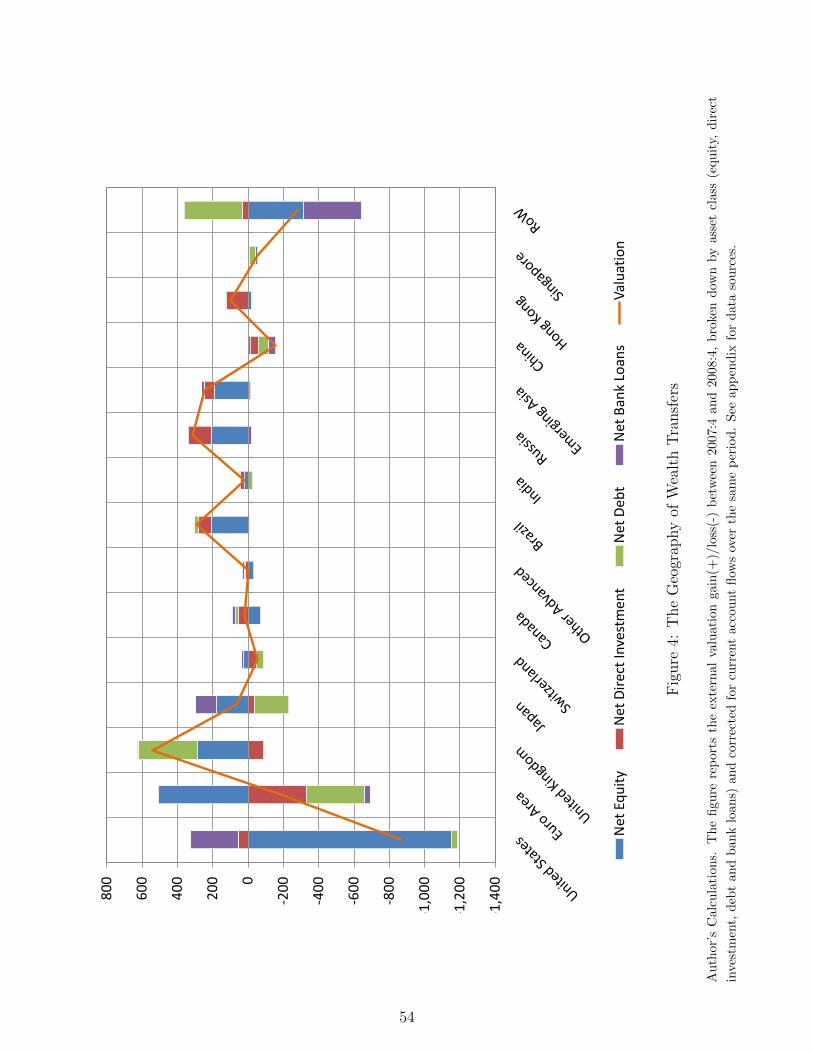
-1,4

00

-1,2

00

-1,0

00

-800

-600

-400

-2000

200

400

600

800

Net

Equ

ityN

et D

irect

Inve

stm

ent

Net

Deb

tN

et B

ank

Loan

sVa

luat

ion

Fig

ure

4:T

he

Geo

grap

hy

ofW

ealt

hT

ransf

ers

Au

thor

’sC

alcu

lati

ons.

Th

efi

gure

rep

orts

the

exte

rnal

valu

atio

nga

in(+

)/lo

ss(-

)b

etw

een

2007

:4an

d20

08:4

,b

roke

nd

own

by

asse

tcl

ass

(equ

ity,

dir

ect

inve

stm

ent,

deb

tan

db

ank

loan

s)an

dco

rrec

ted

for

curr

ent

acco

unt

flow

sov

erth

esa

me

per

iod

.S

eeap

pen

dix

for

dat

aso

urc

es.

54

Figure 5: Exposure to ABCP and Portfolio Debt Losses, by country

0

0.1

0.2

0.3

0.4

0.5

0.6

rate of loss on debt assets

share of ABCP in debt assets

LM0PW202.wmfThe figure reports for each country or group the share of ABCP in that country debt claims position in

2007, as well as the rate of loss on debt assets between 2007:4 and 2008:4. Source: Authors’ calculations and

Acharya and Schnabl (2010)

55

Figure 6: Exposure to ABCP and Portfolio Debt Losses, fraction of total

0

0.1

0.2

0.3

0.4

0.5

0.6

share of total outstanding ABCP

share of total  loss

LM0PW203.wmfThe figure reports for each country or group the share of ABCP in total ABCP hholdings in 2007, as well

as the share of overall loss on debt assets between 2007:4 and 2008:4. Source: Authors’ calculations and

Acharya and Schnabl (2010)

56

Figure 7: Dollar Shortage and ABCP exposure

500

1000

1500

2000

2500

0

USD shortage (Office) USD shortage (Group) ABCP exposure (100mil USD)

The figure reports the upper limit of the dollar shortage measures constructed at the office and group level

together with ABCP exposure data at the country level. Source: McGuire and von Peter (2009) and Acharya

and Schnabl (2010)

57

Figure 8: Regulatory Environment and Valuation Losses

200

250

300

100

150

200

‐50

0

50

200

‐150

‐100

‐200

Valuation losses Regulatory Quality

The figure reports the index of regulatory quality from Kaufmann, Kraay and Mastruzzi (2010), together

with total valuation losses (+) or gains (-)

58