NATIONAL BANK OF POLAND WORKING PAPER No. 109 - ssl.nbp… · NATIONAL BANK OF POLAND WORKING PAPER...

Bayesian evaluation of DSGE models with financial frictions

Warsaw 2012

Michał Brzoza-Brzezina, Marcin Kolasa

NATIONAL BANK OF POLANDWORKING PAPER

No. 109

Design:

Oliwka s.c.

Layout and print:

NBP Printshop

Published by:

National Bank of Poland Education and Publishing Department 00-919 Warszawa, 11/21 Świętokrzyska Street phone: +48 22 653 23 35, fax +48 22 653 13 21

© Copyright by the National Bank of Poland, 2012

ISSN 2084–624X

http://www.nbp.pl

Michał Brzoza-Brzezina – National Bank of Poland and Warsaw School of Economics; e-mail: [email protected].

Marcin Kolasa – National Bank of Poland and Warsaw School of Economics; e-mail: [email protected].

This research was financed by the MNiSW grant No. 04/BMN/22/11. The views expressed herein are those of the authors and not necessarily those of the National Bank of Poland or the Warsaw School of Economics. We would like to thank Marco Del Negro, Marek Jarociński, Frank Schorfheide, Frank Smets and Raf Wouters for helpful discussions. This paper benefited also from comments received at the NBP seminar, the EABCN Workshop and the EC2 conference.

WORKING PAPER No. 109 1

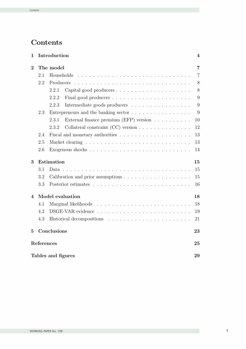
Contents

Contents

1 Introduction 4

2 The model 7

2.1 Households . . . . . . . . . . . . . . . . . . . . . . . . . . . . . . 7

2.2 Producers . . . . . . . . . . . . . . . . . . . . . . . . . . . . . . . 8

2.2.1 Capital good producers . . . . . . . . . . . . . . . . . . . . 8

2.2.2 Final good producers . . . . . . . . . . . . . . . . . . . . . 9

2.2.3 Intermediate goods producers . . . . . . . . . . . . . . . . 9

2.3 Entrepreneurs and the banking sector . . . . . . . . . . . . . . . . 9

2.3.1 External finance premium (EFP) version . . . . . . . . . . 10

2.3.2 Collateral constraint (CC) version . . . . . . . . . . . . . . 12

2.4 Fiscal and monetary authorities . . . . . . . . . . . . . . . . . . . 13

2.5 Market clearing . . . . . . . . . . . . . . . . . . . . . . . . . . . . 13

2.6 Exogenous shocks . . . . . . . . . . . . . . . . . . . . . . . . . . . 14

3 Estimation 15

3.1 Data . . . . . . . . . . . . . . . . . . . . . . . . . . . . . . . . . . 15

3.2 Calibration and prior assumptions . . . . . . . . . . . . . . . . . . 15

3.3 Posterior estimates . . . . . . . . . . . . . . . . . . . . . . . . . . 16

4 Model evaluation 18

4.1 Marginal likelihoods . . . . . . . . . . . . . . . . . . . . . . . . . 18

4.2 DSGE-VAR evidence . . . . . . . . . . . . . . . . . . . . . . . . . 19

4.3 Historical decompositions . . . . . . . . . . . . . . . . . . . . . . 21

5 Conclusions 23

References 28

Tables and figures 29

1

Contents

1 Introduction 4

2 The model 7

2.1 Households . . . . . . . . . . . . . . . . . . . . . . . . . . . . . . 7

2.2 Producers . . . . . . . . . . . . . . . . . . . . . . . . . . . . . . . 8

2.2.1 Capital good producers . . . . . . . . . . . . . . . . . . . . 8

2.2.2 Final good producers . . . . . . . . . . . . . . . . . . . . . 9

2.2.3 Intermediate goods producers . . . . . . . . . . . . . . . . 9

2.3 Entrepreneurs and the banking sector . . . . . . . . . . . . . . . . 9

2.3.1 External finance premium (EFP) version . . . . . . . . . . 10

2.3.2 Collateral constraint (CC) version . . . . . . . . . . . . . . 12

2.4 Fiscal and monetary authorities . . . . . . . . . . . . . . . . . . . 13

2.5 Market clearing . . . . . . . . . . . . . . . . . . . . . . . . . . . . 13

2.6 Exogenous shocks . . . . . . . . . . . . . . . . . . . . . . . . . . . 14

3 Estimation 15

3.1 Data . . . . . . . . . . . . . . . . . . . . . . . . . . . . . . . . . . 15

3.2 Calibration and prior assumptions . . . . . . . . . . . . . . . . . . 15

3.3 Posterior estimates . . . . . . . . . . . . . . . . . . . . . . . . . . 16

4 Model evaluation 18

4.1 Marginal likelihoods . . . . . . . . . . . . . . . . . . . . . . . . . 18

4.2 DSGE-VAR evidence . . . . . . . . . . . . . . . . . . . . . . . . . 19

4.3 Historical decompositions . . . . . . . . . . . . . . . . . . . . . . 21

5 Conclusions 23

References 28

Tables and figures 29

1

N a t i o n a l B a n k o f P o l a n d2

List of Tables and Figures

List of Tables

1 Calibrated parameters . . . . . . . . . . . . . . . . . . . . . . . . 29

2 Priors for estimated parameters . . . . . . . . . . . . . . . . . . . 30

3 Estimation results: DSGE . . . . . . . . . . . . . . . . . . . . . . 31

4 Marginal likelihood comparison . . . . . . . . . . . . . . . . . . . 31

5 Estimation results: DSGE-VAR . . . . . . . . . . . . . . . . . . . 32

6 Decomposition of output contraction during US recessions . . . . 33

List of Figures

1 Monetary shock IRFs . . . . . . . . . . . . . . . . . . . . . . . . . 34

2 Productivity shock IRFs . . . . . . . . . . . . . . . . . . . . . . . 35

3 Preference shock IRFs . . . . . . . . . . . . . . . . . . . . . . . . 36

4 Net worth / LTV shock IRFs . . . . . . . . . . . . . . . . . . . . 37

5 Riskiness / spread shock IRFs . . . . . . . . . . . . . . . . . . . . 38

6 Decomposition of output growth: NK . . . . . . . . . . . . . . . . 39

7 Decomposition of output growth: EFP . . . . . . . . . . . . . . . 40

8 Decomposition of output growth: CC . . . . . . . . . . . . . . . . 41

2

Abstract


Abstract

We evaluate two most popular approaches to implementing financial fric-

tions into DSGE models: the Bernanke et al. (1999) setup, where financial

frictions enter through the price of loans, and the Kiyotaki and Moore

(1997) model, where they concern the quantity of loans. We take both

models to the US data and check how well they fit it on several margins.

Overall, comparing the models favors the framework of Bernanke et al.

(1999). However, even this model is not able to make a clear improvement

over the benchmark New Keynesian model, and the Kiyotaki and Moore

(1997) underperforms it on several margins. Furthermore, none of the

extensions explains the 2007-09 recession as significantly more “financial”

than several previous ones.

JEL: E30, E44

Keywords: financial frictions, DSGE models, DSGE-VAR, Bayesian anal-

ysis

3

Introduction


1

1 Introduction

One of the consequences of the financial crisis 2007-09 was the emergence of

widespread interest in macroeconomic models featuring financial frictions and

disturbances. Economists acknowledged that financial sector imperfections are

necessary for both explaining economic developments and designing appropriate

stabilization policies. Studies addressing the former topic concern i.a. the role

of financial frictions in monetary transmission (Calza et al., 2009; Gerali et al.,

2010; Christiano et al., 2010) or the impact of financial shocks on the economy

(Christiano et al., 2003; Iacoviello and Neri, 2010; Brzoza-Brzezina and Makarski,

2011). As regards the latter area, one can mention papers analyzing optimal

monetary policy in the presence of financial frictions (Curdia and Woodford,

2008; De Fiore and Tristani, 2009; Carlstrom et al., 2010; Kolasa and Lombardo,

2011) or the consequences of capital regulations and macroprudential policies

(Angelini et al., 2010; Angeloni and Faia, 2009; Meh and Moran, 2010; deWalque

et al., 2010).

A dominant part of the financial frictions literature builds on two approaches

developed long before the crisis. The first originates from the seminal paper of

Bernanke and Gertler (1989), where financial frictions have been incorporated

into a general equilibrium model. This approach was further developed by Carl-

strom and Fuerst (1997) and merged with the New Keynesian framework by

Bernanke et al. (1999), becoming the workhorse financial accelerator model in

the 2000s. In this model, frictions arise because monitoring a loan applicant is

costly, which drives an external finance premium (henceforth EFP) between the

lending rate and the risk free rate.

The second direction was introduced by Kiyotaki and Moore (1997) and ex-

tended by Iacoviello (2005). This line of research introduces financial frictions

via collateral constraints (henceforth CC). Agents are heterogeneous in terms of

their rate of time preference, which divides them into lenders and borrowers. The

financial sector intermediates between these groups and introduces frictions by

requiring that borrowers provide collateral for their loans. Hence, this approach

introduces frictions that affect directly the quantity of loans, rather than their

price, as in the Bernanke et al. (1999) setup.

What follows is a situation where important policy conclusions are derived

from two different modeling frameworks. While in economic sciences such a

situation is neither rare nor necessarily unwelcome, still it seems important to

understand what the alternative modeling assumptions imply and how close they

4

Introduction


1

come to reality. This evidence is still scarce. In a recent study Brzoza-Brzezina

et al. (2011) compare the calibrated versions of the EFP and CC frameworks,

finding that the business cycle properties of the former are more in line with

empirical evidence.

In this paper we take the models directly to the data, estimate them using

the Bayesian approach and evaluate their fit as well as power to explain the

past. Several recent papers have looked at the performance and implications of

estimated DSGE models with financial frictions. Christensen and Dib (2008)

estimate an EFP-type model for the US using a maximum-likelihood procedure

and find that the financial accelerator mechanism is supported by the data. This

result was confirmed for both US and euro area data by Queijo von Heideken

(2009) using Bayesian methods. Christiano et al. (2010) augment the standard

New Keynesian model with an EFP-like financial accelerator and the banking

sector similar to Chari et al. (1995), and estimate it on euro area and US ob-

servations. They feed their model with a number of various shocks, estimate it

using Bayesian methods, and document its reasonable fit. The empirical litera-

ture using CC-like models is relatively scarce. A prominent example is Gerali et

al. (2010), who estimate a model of such type, augmented by a housing sector

and a bank balance sheet channel, using Bayesian inference and data for the euro

area. However, they do not discuss whether their framework improves over the

standard New Keynesian setup.

All these papers have studied only one of the two aforementioned ways of in-

troducing financial frictions. As they are also heterogeneous in terms of modeling

choices and data used, they leave no clue on which type of frictions better fits the

data. In this paper, we contribute to the literature by estimating the alternative

financial frictions frameworks, tweaked in a way that allows for both qualitative

and quantitative comparisons. Another important gap in the existing literature

is that it compares models with and without financial frictions relying on esti-

mations performed without the use of financial data. We find this awkward and

hence propose ways of comparing the models estimated also with financial time

series (loans and spreads).

Our main findings are as follows. Evidence from marginal likelihoods shows

that the EFP model is more in line with the data than the CC framework. More-

over, the CC framework performs even worse than the frictionless New Keynesian

benchmark. As to the EFP model, the evidence is mixed: in some exercises it

performs somewhat better than the New Keynesian model, in others worse. Defi-

nitely, a clear improvement cannot be observed. The evidence from DSGE-VARs

5

Introduction


1

shows that both financial friction frameworks are seriously misspecified and do

not improve in this respect upon the standard New Keynesian model. Moreover,

while both extensions give a substantial role to financial disturbances in explain-

ing the business cycle, surprisingly they are not able to identify the 2007-09 crisis

to be more“financial” in nature (i.e. driven to a larger extent by financial shocks)

than several previous recessions. This feature is particularly acute for the CC

model and stands in sharp contrast with common knowledge, supported by em-

pirical findings, that the origins of the recent crisis can be traced to the financial

sector (Brunnermeier, 2009; Gilchrist and Zakrajcek, 2011; Gorton, 2009).

In our view, these results suggests that relying on any of the two standard

financial accelerator setups is not sufficient for explaining the recent financial

crisis and designing tools that could help avoiding similar ones in the future. The

currently observed ongoing development of alternative and more sophisticated

frameworks, such as more explicit modeling of financial intermediation (Gertler

and Kiyotaki, 2010; Gertler and Karadi, 2011) or allowing for occasionally rather

than eternally binding collateral constraints (Brunnermeier and Sannikov, 2011;

Jeanne and Korinek, 2010; Mendoza, 2010), seems to be a necessary step.

The rest of the paper is structured as follows. Section 2 introduces the New

Keynesian model and its two alternative extensions featuring two types of fi-

nancial frictions. In Section 3 we discuss their estimation. Section 4 evaluates

the models, documents their misspecification and shows their implications for

historical decompositions. Section 5 concludes.

6

The model


2

2 The model

Our departure point is a standard medium-sized closed economy New Key-

nesian (henceforth NK) model with sticky prices and a standard set of other

frictions that have been found crucial for ensuring a reasonable empirical fit (see

Christiano et al., 2005; Smets and Wouters, 2003). Such a model economy is

populated by households, producers, as well as fiscal and monetary authorities.

Households consume, accumulate capital stock and work. Output is produced in

several steps, including a monopolistically competitive sector with producers fac-

ing price rigidities. Fiscal authorities use lump sum taxes to finance government

expenditure and monetary authorities set the short-term interest rate according

to a Taylor rule.

To introduce financial frictions, this setup is modified by including two new

types of agents: entrepreneurs and the banking sector. Entrepreneurs specialize

in capital management. They finance their operations, i.e. renting capital ser-

vices to firms, by taking loans from the banking sector, which refinances them

by accepting deposits from households. It is this intermediation where financial

frictions arise and their nature differs between the EFP and CC variants. The

standard NK model obtains as a special case of either of the two alternative

extensions.

In the EFP version, financial frictions originate from riskiness in management

of capital and asymmetric information. Individual entrepreneurs are subject to

idiosyncratic shocks, which are observed by them for free, while banks can learn

about the shocks’ realizations only after paying monitoring costs. This costly

state verification problem results in a financial contract featuring an endogenous

premium between the lending rate and the risk-free rate.

The key financial friction in the CC version is introduced by assuming that

entrepreneurs need collateral to take a loan. Additionally, to ensure comparabil-

ity with the EFP version, we assume that the interest rate on loans differs from

the risk-free rate due to monopolistic competition in the banking sector.

In the rest of this section we lay down the model, highlighting the differences

between the three specifications.

2.1 Households

The economy is populated by a continuum of households indexed by h. Each

household chooses consumption ct and labor supply nt to maximize the expected

7

The model


2

lifetime utility

E0

∞∑t=0

βt

[Γt

(ct (h)− ξct−1)1−σc

1− σc

− nt (h)1+σn

1 + σn

](1)

where ξ denotes the degree of external habit formation and Γt is a preference

shock. Each household uses labor income Wtnt, capital income Rk,tkt−1 and div-

idends Πt to finance its expenditure and lump sum taxes Tt, facing the following

budget constraint

Ptct (h) + Et {Υt+1Bt (h)} ≤ Wtnt (h)− Tt (h) + Πt (h) + Bt−1 (h) (2)

where Pt denotes the price of a consumption good. As in Chari et al. (2002),

we assume that households have access to state contingent bonds Bt, traded at

price Υt,t+1, which allows them to insure against idiosyncratic risk. The expected

gross rate of return [Et{Υt+1}]−1 is equal to the risk-free interest rate Rt, fully

controlled by the monetary authority.

Each household has a unique labor type h, which is sold to perfectly compet-

itive aggregators, who pool all labor types into one undifferentiated labor service

with the following function

nt =

(ˆ 1

0

nt (h)1

φw dh

)φw

(3)

Households set their wage rate according to the standard Calvo scheme. With

probability (1− θw) they receive a signal to reoptimize and then set their wage

to maximize the utility, subject to the demand from the aggregators. Those who

do not receive the signal index their wage to the weighted average of past and

steady state inflation, with the weight on the former denoted by ζw.

2.2 Producers

There are several stages of production in the economy. Intermediate goods

firms produce differentiated goods and sell them to aggregators. Aggregators

combine differentiated goods into a homogeneous final good. The final good can

be used for consumption or sold to capital good producers.

2.2.1 Capital good producers

Capital good producers act in a perfectly competitive environment. In each

8

The model


2

period a representative capital good producer buys it of final goods and old

undepreciated capital (1− δ) kt−1. Next she transforms old undepreciated capital

one-to-one into new capital, while transformation of the final good is subject to

an adjustment cost S (it/it−1).1 Thus, the technology to produce new capital is

given by

kt = (1− δ) kt−1 +

(1− S

(itit−1

))it (4)

The new capital is then sold in a perfectly competitive market. The price of

capital is denoted by Qt.

2.2.2 Final good producers

Final good producers play the role of aggregators. They buy differentiated

products from intermediate goods producers y (j) and aggregate them into a

single final good, which they sell in a perfectly competitive market. The final

good is produced according to the following technology

yt =

(ˆ 1

0

yt (j)1φ dj

)φ

(5)

2.2.3 Intermediate goods producers

There is a continuum of intermediate goods producers indexed by j. They

rent capital and labor and use the following production technology

yt(j) = Atkt(j)αnt(j)

1−α (6)

where At is total factor productivity.

Intermediate goods firms act in a monopolistically competitive environment

and set their prices according to the standard Calvo scheme. In each period each

producer receives with probability (1− θ) a signal to reoptimize and then sets

her price to maximize the expected profits, subject to demand schedules implied

by final goods producers’ optimization problem. Those who are not allowed to

reoptimize index their prices to the weighted average of past and steady state

inflation, with the weight on the former denoted by ζ.

2.3 Entrepreneurs and the banking sector

The specification of entrepreneurs and the financial sector differs between the

EFP and CC versions, so we present them in two separate subsections.

1We adopt the specification of Christiano et al. (2005) and assume that S (1) = S′(1) = 0

and S′′(1) = κ > 0.

9

The model


2

2.3.1 External finance premium (EFP) version

There is a continuum of risk-neutral entrepreneurs, indexed by ι. At the end

of period t, each entrepreneur purchases installed capital kt(ι) from capital pro-

ducers, partly using her own financial wealth Vt(ι) and financing the remainder

with a bank loan Lt(ι)

Lt(ι) = Qtkt(ι)− Vt(ι) ≥ 0 (7)

After the purchase, each entrepreneur experiences an idiosyncratic productivity

shock, which converts her capital to aE(ι)kt(ι), where aE is a random variable,

distributed independently over time and across entrepreneurs, with a cumulative

density function F (ι) and a unit mean. Following Christiano et al. (2003), we

assume that this distribution is log normal, with a stochastic standard deviation

of log aE equal to σaE ,t.

Next, each entrepreneur rents out capital services, treating the rental rate

Rk,t+1 as given. The average rate of return on capital earned by entrepreneurs is

RE,t+1 ≡Rk,t+1 + (1− δ)Qt+1

Qt

(8)

and the rate of return earned by an individual entrepreneur is aE(ι)RE,t+1.

Since lenders can observe the return earned by borrowers only at a cost, the

optimal contract between these two parties specifies the size of the loan Lt(ι) and

the gross non-default interest rate RL,t+1(ι). The solvency criterion can also be

defined in terms of a cutoff value of idiosyncratic productivity, denoted as aE,t+1,

such that the entrepreneur has just enough resources to repay the loan

aE,t+1RQtkt(ι) = RL,t+1(ι)Lt(ι) (9)

Entrepreneurs with aE below the threshold level go bankrupt. All their resources

are taken over by the banks, after they pay a proportional monitoring cost µ.

Banks finance their loans by issuing time deposits to households at the risk-

free interest rate Rt. The banking sector is assumed to be perfectly competitive

and owned by risk-averse households. This, together with risk-neutrality of en-

trepreneurs implies that an optimal financial contract insulates the lender from

any aggregate risk.2 Hence, interest paid by entrepreneurs is state contingent

and guarantees that banks break even in every period.

2Given the infinite number of entrepreneurs, the risk arising from idiosyncratic shocks isfully diversifiable.

10

The model


2

The equilibrium debt contract maximizes welfare of each individual entrepreneur,

defined in terms of expected end-of-contract net worth relative to the risk-free

alternative

Et

{´∞aE,t

(RE,t+1Qtkt(ι)aE(ι)−RL,t+1Lt(ι)) dF (aE(ι))

RtVt(ι)

}(10)

subject to banks’ zero profit condition. The solution to this problem (after

dropping the expectations operator) is an endogenous and identical to all en-

trepreneurs wedge χEFP between the rate of return on capital and the risk free

rate

RE,t+1 = (1 + χEFP (aE,t+1))Rt (11)

It can be verified that if µ = 0, i.e. monitoring by banks is free, then χEFP = 0,

financial markets work without frictions and the EFP variant simplifies to the

standard NK setup.

Entrepreneurs’ optimization also implies that the non-default interest rate

(common to all entrepreneurs) is

RL,t+1 =aE,t+1RE,t+1Qtkt(ι)

Qtkt(ι)− Vt(ι)(12)

Proceeds from selling capital, net of interest paid to the banks, constitute end

of period net worth. To ensure that entrepreneurs do not accumulate enough

wealth to become fully self-financing, it is assumed that each period a randomly

selected and stochastic fraction (1−νt) of them go out of business, in which case

all their financial wealth is rebated to the households. At the same time, an equal

number of new entrepreneurs enters so that their total number is constant. Those

who survive or enter receive a fixed transfer TE from households. This ensures

that entrants have at least a small but positive amount of wealth, without which

they would not be able to buy any capital.

Aggregating across all entrepreneurs yields the following law of motion for

net worth in the economy

Vt = νt

[RE,tQt−1kt−1 −

(Rt−1 +

µF2,tRE,tQt−1kt−1

Lt−1

)Lt−1

]+ TE (13)

where

11

The model


2

F2,t ≡ˆ aE,t

0

aEdF (aE) (14)

2.3.2 Collateral constraint (CC) version

There is a continuum of entrepreneurs, indexed by ι. They draw utility only

from their consumption cEt

E0

∞∑t=0

βtE

(cEt (ι)− ξcEt−1

)1−σc

1− σc

(15)

Entrepreneurs cover consumption and capital expenditures with revenues from

renting capital services to intermediate goods producers, financing the remainder

by bank loans Lt, on which the interest to pay is RL,t

PtcEt (ι)+Qtkt(ι)+RL,t−1Lt−1 (ι)+ TE = (Rk,t +Qt (1− δ)) kt−1 (ι)+Lt (ι) (16)

where TE denotes fixed transfers between households and entrepreneurs. Loans

taken by the entrepreneurs are subject to the following collateral constraint

RL,tLt (ι) ≤ mtEt [Qt+1 (1− δ) kt (ι)] (17)

where mt is the loan-to-value ratio. Since we assume that βE < β, the constraint

is binding as long as the economy does not deviate too much from its steady

state.

The banking system consists of monopolistically competitive banks and finan-

cial intermediaries operating under perfect competition. This two-stage structure

is necessary to introduce time-varying interest rate spreads.

Financial intermediaries take differentiated loans from banks Lt (i) at the

interest rate RL,t(i) and aggregate them into one undifferentiated loan Lt that is

offered to entrepreneurs at the rate RL,t. The technology for aggregation is

Lt =

[ˆ 1

0

Lt (i)1

φL,t di

]φL,t

(18)

where φL,t is a stochastic measure of substitutability between loan varieties.

Each bank i collects deposits Dt (i) from households at the risk-free rate Rt,

and uses them for lending to financial intermediaries. Banks set their interest

12

The model


2

rates to maximize profits subject to the demand for loans from the financial

intermediaries.

Solving the problem of entrepreneurs, banks and financial intermediaries

yields the following analog to (11) from the EFP variant

RE,t+1 = (1 + ΘtχCC(mt,Qt+1, Qt,Rk,t+1))φL,tRt (19)

where χCC > 0 and Θ is the Lagrange multiplier on constraint (17). As can

be seen, the collateral constraint and monopolistic competition in the banking

industry drive a wedge between the return on capital and the (risk-free) policy

rate. If the collateral constraint is not binding (Θt = 0) and the banking industry

is perfectly competitive (φL,t = 1), then financial frictions disappear, making the

CC variant equivalent to the standard NK setup.

2.4 Fiscal and monetary authorities

The government uses lump sum taxes to finance its expenditure gt. We

assume that the budget is balanced each period so that gt = Tt.

As it is common in the New Keynesian literature, we assume that monetary

policy is conducted according to a Taylor rule that targets deviations of inflation

and output from the deterministic steady state, allowing additionally for interest

rate smoothing

Rt =

(Rt−1

R

)γR((πt

π

)γπ(yty

)γy)1−γR

eϕt (20)

where πt ≡ Pt/Pt−1, a bar over a variable denotes its steady state value and ϕt

is the monetary shock.

2.5 Market clearing

The market clearing condition for the final goods market differs between

our three model variants. In the EFP variant, it must take into account that

monitoring costs are real, which results in the following formula

ct + it + gt + µF2,tRE,tqt−1kt−1 = yt (21)

The counterpart of (21) in the CC variant includes entrepreneurs’ consumption

ct + it + gt + cEt = yt (22)

By dropping monitoring costs from (21) or entrepreneurs’ consumption from (22),

13

The model


2

we obtain the market clearing condition for the standard NK model.

2.6 Exogenous shocks

Business cycle fluctuations in the simplest version of our model (NK) are

driven by shocks to productivity (At), households’ preferences (Γt) and Taylor

rule (ϕt). They are the standard representatives of stochastic disturbances to

supply, demand and monetary policy. Each of the financial extensions includes

two more shocks related to the financial sector. In the EFP variant, these are

the standard deviation of idiosyncratic productivity (σaE ,t) and the exit rate for

entrepreneurs (νt). We will refer to them as riskiness and net worth shocks,

respectively. In the CC version, the two additional shocks are the LTV ratio

(mt) and markup in financial intermediation (φL,t), the latter referred to as a

spread shock. The log of each shock follows a linear first-order autoregressive

process, except for the monetary policy shock, which is assumed to be white

noise.

14

Estimation


3

3 Estimation

3.1 Data

We estimate the log-linearized approximations of all three model versions

laid down in the previous section using Bayesian inference. We use quarterly US

data spanning the 1970-2010 period. In the NK model, the observable variables

are the standard three macroeconomic time series: real GDP, CPI inflation and

the federal funds rate. In the EFP and CC variants, we additionally use two

financial variables, i.e. real loans to firms and spread on loans to firms, both

defined as in Christiano et al. (2010). More specifically, the former is credit

market instruments liabilities of nonfarm nonfinancial businesses, taken from

the Flow of Funds Account of the Federal Reserve Board and deflated with the

GDP deflator. The latter is the difference between the industrial BBB corporate

bond yield, backcasted using BAA corporate bond yields (both series taken from

Bloomberg), and the federal funds rate. Trending data (GDP and loans) are

made stationary by removing a linear trend from their logs, while the interest

rate, inflation and the spread are demeaned.

3.2 Calibration and prior assumptions

As it is common in the applied DSGE literature, we keep a number of param-

eters fixed in the estimation.3 These are the parameters that affect the steady

state proportions in our models and hence most of them cannot be pinned down

in the estimation procedure that uses detrended or demeaned observable vari-

ables. An additional advantage of calibrating this subset of parameters is that it

can be done such that the steady state solutions of our competing models with

financial frictions are identical, which facilitates comparisons. The results of our

calibration are presented in Table 1.

We calibrate the structural parameters unrelated to the financial sector (and

so common across the NK, EFP and CC versions) by taking their values directly

from the previous literature, relying mainly on Smets and Wouters (2007), or set

them to match the key steady state proportions of the US data. As regards the

calibrated parameters specific to the EFP or CC extensions, we apply the same

procedure as in Brzoza-Brzezina et al. (2011), the details of which are presented

3Both Bayesian estimation of DSGE models and fixing part of the parameters are standardin the literature (e.g. Smets and Wouters (2003); Adolfson et al. (2005)). This procedurefollows the observation that for many parameters the likelihood function is almost flat. In sucha case either imposing a tight prior or fixing some of the parameters is necessary to estimatethe model.

15

Estimation


3

below.

In each of our extensions to the NK setup, the financial sector is governed

by four parameters. These parameters are µ, ν, σaE , TE in the EFP model

and βE, φL, m, TE in the CC variant. We use them to pin down four steady

state proportions: investment share in output, interest rate spread, capital to

debt ratio and the output share of monitoring costs (EFP) / entrepreneurs’

consumption (CC). The first three have their natural empirical counterparts,

which we match exactly. In particular, our calibration implies that in the steady

state around half of capital is financed by loans (Bernanke et al., 1999) and the

annualized spread is 88 basis points (the average in our data). The target value

for the share of monitoring costs / entrepreneurs’ consumption is set to 0.5%,

which is consistent with Christiano et al. (2010). As a result, our calibration

implies that the steady state rate of return on capital, and hence the excess

return on capital defined by equations (11) and (19), are the same in the EFP

and CC versions.

The remaining model parameters are estimated. Our prior assumptions are

summarized in Table 2. Overall, they are consistent with the previous literature

(e.g. Smets and Wouters, 2007) and relatively uninformative.

3.3 Posterior estimates

The posterior estimates are reported in Table 3.4 They are obtained using

the Metropolis-Hastings algorithm. We ran 1,000,000 draws from two chains,

burning the first half of each chain. The stability of thus obtained sample was

assessed using the convergence statistics proposed by Brooks and Gelman (1998).

Our parameter estimates for the NK model are in line with the related DSGE

literature based on US data. In particular, the posterior means of parameters

describing nominal and real rigidities, i.e. Calvo probabilities and indexation in

prices and wages as well as investment adjustment costs, nearly coincide with

those obtained by Smets and Wouters (2007). This is despite the fact that we

use a narrower set of observable variables and shocks.

Adding financial frictions to the NK setup changes the estimates of some of

these parameters significantly. First, prices appear to be more sticky (higher θ)

according to the EFP model, while the opposite holds true for the CC variant.

Together with a relatively low estimate of the Calvo probability for wages θw in

the CC model, this result suggests that, compared to the standard NK model,

one needs more (less) nominal rigidities in the EFP (CC) setup to account for

4All estimations in this paper are done with Dynare (www.dynare.org).

16

Estimation


3

sensitivity of inflation to real activity observed in the data. Second, the esti-

mated curvature of the investment adjustment cost function κ in the EFP model

is significantly smaller than that in the baseline NK model or the CC extension.

This finding is consistent with Brzoza-Brzezina et al. (2011), who point at rela-

tively strong propagation of shocks on real variables in the EFP setup, especially

in comparison to the CC model.

Differences in the degree of nominal rigidities across the three model variants

translate into differences in the estimates of the monetary policy feedback rules.

In particular, more (less) wage or price stickiness in the EFP (CC) variant com-

pared to the NK baseline implies a less (more) aggressive response of the interest

rate to inflation to ensure its volatility at the level close to observed in the data.

We know from the earlier literature that structural shocks in estimated DSGE

models usually exhibit high persistence. This may signal misspecification, an

issue we address in the next sections. According to our results, high shock

inertia is particularly pronounced in the CC model. In particular, the mean

posterior estimate of autocorrelation of productivity, preference and LTV shocks

are around 0.95 and relatively tightly estimated.

17

Model evaluation


4

4 Model evaluation

4.1 Marginal likelihoods

As a first step we compare the data fit of the three frameworks. In a Bayesian

setting, a natural measure for model comparisons is marginal likelihood. How-

ever, comparisons of marginal likelihoods (calculation of the posterior odds ra-

tios) are valid only if the evaluated models are estimated with the same data

sets. Since in our baseline setting this is not the case (the NK model is esti-

mated without financial variables), we take a number of alternative approaches

that help us circumvent this problem. The results which we refer to are collected

in Table 4.

As a first step we reestimate the models on data sets containing only non-

financial variables (i.e. output, inflation and the interest rate). This is done in

two variants. The first row presents marginal likelihoods for the models described

in Section 2. Clearly the best performing model is EFP. Adding financial frictions

of this type to the NK model helps in bringing it closer to the data. However, to

our surprise, the CC model underperforms the NK model. This type of frictions

seems not to be accepted. The second row provides the results of a somewhat

modified exercise, where we remove financial shocks from the financial friction

models. This is intended to make the “competition” more fair towards the NK

model, since additional shocks can be expected to improve the fit. Moreover, the

exercise becomes closest to those performed in the literature (Christensen and

Dib, 2008; Queijo von Heideken, 2009), where the financial accelerator model of

Bernanke et al. (1999) has been found to outperform its frictionless version. Re-

moving financial shocks lowers the marginal likelihoods of both financial friction

frameworks, but does not affect the ordering. Consistently with the literature,

the EFP framework performs best (though the gain over the NK model becomes

very small). Again, the CC model performs worst.

While this exercise is telling, one could (as we do) find evaluating financial

friction models without using financial data somewhat unfair. For this reason,

we embark on another exercise, that allows for the comparison of all models. To

this end, we enlarge the NK model for the presence of financial variables. As this

model does not feature financial variables, this is done in a non-structural way

- we assume simple time series processes that drive the two financial variables.

In particular we introduce them as either first-order (third row) or second-order

(fourth row) autoregressive processes. In the former case we assume priors as for

18

Model evaluation


4

shocks, in the latter we allow the coefficients on the lags to fall outside the unit

interval and hence assume normal rather than beta prior distributions, centered

around 0.5 (first lag) and 0 (second lag). As evidenced in Smets and Wouters

(2007), the DSGE framework can outperform time series models (Bayesian VARs

in particular) in terms of marginal likelihood. Against this background our ev-

idence is striking. While the NK model augmented by a simple AR(1) specifi-

cation for financial variables performs worse than the financial friction models,

allowing for just one additional lag in the atheoretical part makes the NK setup

perform substantially better than both the CC and EFP frameworks. Addition-

ally, one could note that the superior performance of the EFP model over CC

remains valid after inclusion of financial variables.

All in all, the evidence from comparisons of the marginal likelihoods casts

clear doubt over the performance of the CC framework. The improvement from

introducing EFP type frictions is also less clear than hitherto documented in the

literature, not using financial variables in estimation.

4.2 DSGE-VAR evidence

Another method used in the literature for comparison of DSGE models are

DSGE-VARs, put forward by Del Negro and Schorfheide (2004). This framework

has recently become a popular tool for assessing the degree of misspecification

of DSGE models (Del Negro et al., 2007; An and Schorfheide, 2007; Del Negro

and Schorfheide, 2009). The DSGE-VAR approach relies on a simple observation

that a DSGE model can be approximated by a finite order vector autoregression

(VAR). In this case, the VAR parameters are determined by the parameters of

the DSGE model and cross-equation restrictions it implies. In this context, one

can think of relaxing the restrictions imposed by the theoretical model, thus

letting the data influence the VAR to a larger degree.

This is in a nutshell the concept of DSGE-VARs. The estimation of a VAR

model is augmented with prior knowledge, stemming from the DSGE model.

The extent to which the theoretical model influences the VAR coefficients can be

chosen by the researcher by varying a parameter which determines the tightness

of the DSGE-based prior. In what follows this parameter will be denoted as λ.

If λ = 0, an unrestricted VAR is estimated. If λ = ∞, the VAR parameters

approach the restrictions implied by the DSGE model. For λ = 1, the DSGE

prior and the data receive equal weight in the VAR-representation posterior.

We estimate three DSGE-VAR models corresponding to the three alternative

DSGE specifications described above. As in Adjemian et al. (2008), we estimate

19

Model evaluation


4

λ directly, using a flat prior. We will refer to these values as to λ. The results,

obtained using the same parametrization of the Metropolis-Hastings algorithm

as described in section 3.3, are reported in Table 5.

The posterior estimates of λ are very small for all three models, indicating

that the data is consistent with merely a loose DSGE prior. This not only

confirms the result found in the literature that standard New Keynesian models

are seriously misspecified (Del Negro et al., 2007), but also shows that adding

financial frictions does not help solving this problem. In fact, the posterior

means of λ for both financial friction models are even lower than for the NK

model, though it should be added that the overlap in the three relevant posterior

densities is considerable.

This observation finds further support if we look at the evidence from marginal

likelihoods (Table 4). For any model variant, their estimates rise substantially if

we relax the DSGE-based restrictions. Interestingly, the log marginal likelihood

differential between the DSGE model and its DSGE-VAR representation for the

two financial frictions extensions are about four times larger than for the NK

benchmark.

As explained by Del Negro and Schorfheide (2009), the superior data fit of

DSGE-VARs leads to smaller forecast errors and smaller shock volatility esti-

mates. As can be seen from Table 5, this is also the case in our results for

all three model variants. Relaxing the DSGE model restrictions means that

the model misspecification no longer needs to be absorbed by structural shocks,

which results in processes with lower persistence and volatility.

Next, we analyze the misspecification of our three models by comparing their

impulse responses with those from DSGE-VARs. In this respect we proceed

along the lines drawn by Del Negro and Schorfheide (2009) and construct DSGE-

VAR(∞) models, where the structural parameters (including the shock variances

and autocorrelations) have been fixed at their posterior means from the cor-

responding DSGE-VAR(λ)’s, presented in Table 5. As explained in detail in

Del Negro and Schorfheide (2009), such a procedure allows to clear the misspec-

ification of the model from the impact of different parameter estimates. The

results are depicted in Figures 1 to 5.

It should be noted that, with minor exceptions, for any given shock and vari-

able, the DSGE-VAR impulse response functions are similar across the models.

This is consistent with relatively low estimated values of λ and gives support to

treating DSGE-VAR based responses as an empirical benchmark. Given the vast

20

Model evaluation


4

amount of information embedded in the reaction functions, we concentrate on

the main findings.

First, the general impression from analyzing the responses is consistent with

the finding on estimated λ’s. All models seem misspecified to a comparable de-

gree, as all DSGE-VAR(∞) impulse responses often leave the DSGE-VAR(λ)

probability intervals. Second, in spite of the above, in most cases the direction of

the impulse responses in the DSGE-VAR(∞) models and their empirical bench-

marks coincide. Notable exceptions are rising inflation in the EFP model after

a net worth shock and spread reactions discussed below.

Third, in response to a monetary policy shock, output and inflation do not

show enough persistence. The CC model even overrides the small hump-shapes

visible in the NK model, making the impulse response even less in line with the

empirical benchmark. Fourth, the endogenous reaction of spreads is strongly

supported by the data. This points in favor of the EFP formulation over the CC

model, which lacks such a mechanism. Particular attention should be paid to the

reaction of spreads to a monetary policy shock. While in the DSGE-VAR(∞)

spreads rise on impact after a monetary tightening, in its DSGE-VAR(λ) coun-

terpart they initially decline and rise only over time. The latter reaction results

most probably from the stickiness of retail interest rates (as evidenced i.a. by

De Bondt, 2005), which is not included in our frameworks. As shown by Gerali et

al. (2010), this feature can be added to financial friction models relatively easily

by allowing for staggered setting of retail interest rates.

Fifth, in some cases the behavior of loans is somewhat counterintuitive. This

is especially the case in the EFP model, where loans increase after a monetary

policy tightening and decline after a net worth shock. Last but not least, both

financial friction models show rising inflation after a positive shock to riskiness

(EFP) / spreads (CC). Although this result can be easily explained via cost-push

effects of higher loan servicing, they are at odds with the empirical benchmark,

where inflation declines following this kind of shock.

All in all, analyzing the impulse responses paints a picture of financial friction

models whose degree of misspecification is comparable to the NK benchmark.

While in general the theoretical and empirical impulse responses have much in

common, in several cases the former leave the probability bounds around the

latter and in some cases they even differ as to sign.

4.3 Historical decompositions

One of the aims of financial friction models is to explain the role played

21

Model evaluation


4

by financial disturbances in driving the business cycle. We follow this line and

construct historical shock decompositions for all three models and present them

on Figures 6 - 8. For the sake of transparency, we only show data since 2000q1.

Starting with the NK benchmark, it is clear that in this model the business

cycle is driven mainly by preference (demand type) disturbances. This result

is consistent with an 88% share of this shock in the variance decomposition of

output growth. One interesting finding is the negative contribution of monetary

policy shocks to output growth since 2008q4. This reflects the zero lower bound

constraint hit by the Federal Reserve. Since the interest rates could not be

lowered enough, they started to exert a negative impact on GDP. It has to be

noted that our models do not feature exceptional monetary policy tools like

quantitative easing.

As we move to models with financial frictions, financial shocks start playing

a role in determining output fluctuations. In both models financial shocks have a

substantial, though not overwhelming contribution to output decline during the

2007-09 financial crisis. However, surprisingly, the visual evidence suggests that

the recent recession was not necessarily more “financial” in nature than the 2001

slowdown.

To explore this observation in detail, in Table 6 we present the shock de-

composition of output contraction during US recessions since 1970. Again, the

dominant role of preference shocks evident in the NK model declines to the

benefit of financial shocks in the EFP and CC frameworks. Financial shocks

contributed to the decline of GDP during each NBER recession and, in line with

intuition, their most significant impact on output was during the recent financial

crisis. This conclusion, however, does not hold any more if we control for the size

of recession. The relative role of financial shocks varies from 20% (EFP model,

1970 recession) to 69% (CC model, 1980 recession).5 In this metric, the role

of financial shocks during the financial crisis 2007-09 ranks second for the EFP

model and only fifth for the CC model. This feature stands in sharp contrast

with common knowledge, supported by empirical findings, that the origins of the

recent crisis can be traced to the financial sector (Brunnermeier, 2009; Gilchrist

and Zakrajcek, 2011; Gorton, 2009).

5The latter finding seems consistent with the result obtained by Jermann and Quadrini(2012) in a framework similar to our CC model, who report a low relative contribution offinancial shocks to the development of output during the financial crisis.

22

Conclusions


5

5 Conclusions

After the financial crisis 2007-09, models featuring financial frictions are

promptly entering into the mainstream of macromodeling. They have been used

i.a. to analyze the financial crisis or to speak about optimal monetary policy

in the presence of financial frictions. More importantly, however, these models

are being used to analyze the consequences of capital regulations and to deliver

policy advice on central banks’ macroprudential policies. This calls for a thor-

ough investigation whether they are able to reflect factual economic developments

rather than creating a fictitious world of financial imperfections.

To this end, we conduct an empirical evaluation of the two most popular

macrofinancial frameworks: the external finance premium framework of Bernanke

et al. (1999) and the collateral constraint model of Kiyotaki and Moore (1997).

We estimate their comparable versions on US data together with the bench-

mark New Keynesian model. For each model we also estimate its DSGE-VAR

representation. Our findings are as follows.

First, the comparison of marginal likelihoods clearly favors the Bernanke et al.

framework over the Kiyotaki and Moore model. However, the former improves

upon the benchmark New Keynesian models without financial frictions only in

some settings, and the latter always performs much worse than the benchmark.

Second, comparison of the DSGEs and DSGE-VARs reveals that all three

models are seriously misspecified. While this result for the New Keynesian model

comes as no surprise and has been described in the literature before, it is striking

that introducing financial frictions does not help to solve this problem. This

conclusion comes not only from the formal comparison of the optimal DSGE-

VAR hyperparameters, but also from the visual inspection of misspecification

revealed by the impulse response functions. Additionally, the latter point at

a number of deficiencies of financial friction models (e.g. overriding the model

inertia by the Kiyotaki and Moore framework, or the strong cost-push effects of

riskiness / spread shocks being at odds with the data).

Third, we look how our models interpret the recent financial crisis against

the background of previous recessions. Surprisingly, we find that the role of

financial shocks in driving the 2007-09 recession was not more pronounced than

in several past contractions. In particular, in this category, the recent recession

ranks second for the Bernanke et al. model and only fifth for the Kiyotaki and

Moore model.

We conclude that both financial friction frameworks show serious deficiencies

23

Conclusions


5

and do not offer clear improvements upon the frictionless benchmark. Further

research is needed to find macrofinancial models that reflect reality better. Most

recent research, featuring i.a. a more explicit modeling of financial intermediation

or introducing occasionally binding constraints seem interesting avenues.

24

References


References

Adjemian, Stephane, Matthieu Darracq Parie‘s, and Stephane Moyen (2008)

‘Towards a monetary policy evaluation framework.’ Working Paper Series 942,

European Central Bank, September

Adolfson, Malin, Stefan Laseen, Jesper Linde, and Mattias Villani (2005)

‘Bayesian estimation of an open economy DSGE model with incomplete pass-

through.’ Working Paper Series 179, Sveriges Riksbank (Central Bank of Swe-

den).

An, Sungbae, and Frank Schorfheide (2007) ‘Bayesian analysis of DSGE models.’

Econometric Reviews 26(2-4), 113–172

Angelini, Paolo, Andrea Enria, Stefano Neri, Fabio Panetta, and Mario

Quagliariello (2010) ‘Pro-cyclicality of capital regulation: is it a problem? how

to fix it?’ Questioni di Economia e Finanza (Occasional Papers) 74, Bank of

Italy, Economic Research Department, October

Angeloni, Ignazio, and Ester Faia (2009) ‘A tale of two policies: Prudential

regulation and monetary policy with fragile banks.’ Kiel Working Papers 1569,

Kiel Institute for the World Economy

Bernanke, Ben S., and Mark Gertler (1989) ‘Agency costs, net worth, and busi-

ness fluctuations.’ American Economic Review 79(1), 14–31

Bernanke, Ben S., Mark Gertler, and Simon Gilchrist (1999) ‘The financial ac-

celerator in a quantitative business cycle framework.’ In Handbook of Macroe-

conomics, ed. J. B. Taylor and M. Woodford, vol. 1 of Handbook of Macroeco-

nomics (Elsevier) chapter 21, pp. 1341–1393

Brooks, Stephen, and Andrew Gelman (1998) ‘Some issues in monitoring con-

vergence of iterative simulations.’ In ‘Proceedings of the Section on Statistical

Computing’ American Statistical Association.

Brunnermeier, Markus K. (2009) ‘Deciphering the liquidity and credit crunch

2007-2008.’ Journal of Economic Perspectives 23(1), 77–100

Brunnermeier, Markus K., and Yuliy Sannikov (2011) ‘A macroeconomic model

with a financial sector.’ mimeo, Princeton University

25

References


Brzoza-Brzezina, Micha�l, and Krzysztof Makarski (2011) ‘Credit crunch in a

small open economy.’ Journal of International Money and Finance 30(7), 1406–

1428.

Brzoza-Brzezina, Micha�l, Marcin Kolasa, and Krzysztof Makarski (2011) ‘The

anatomy of standard DSGE models with financial frictions.’ NBP Working

Papers 80, National Bank of Poland

Calza, Alessandro, Tommaso Monacelli, and Livio Stracca (2009) ‘Housing fi-

nance and monetary policy.’ Working Paper Series 1069, European Central

Bank

Carlstrom, Charles T., and Timothy S. Fuerst (1997) ‘Agency costs, net worth,

and business fluctuations: A computable general equilibrium analysis.’ Amer-

ican Economic Review 87(5), 893–910

Carlstrom, Charles T., Timothy S. Fuerst, and Matthias Paustian (2010) ‘Opti-

mal monetary policy in a model with agency costs.’ Journal of Money, Credit

and Banking 42(s1), 37–70

Chari, V V, Lawrence J Christiano, and Martin Eichenbaum (1995) ‘Inside

money, outside money, and short-term interest rates.’ Journal of Money, Credit

and Banking 27(4), 1354–86

Chari, Varadarajan V., Patrick J. Kehoe, and Ellen R. McGrattan (2002) ‘Can

sticky price models generate volatile and persistent real exchange rates?’ Re-

view of Economic Studies 69(3), pp. 533–63

Christensen, Ian, and Ali Dib (2008) ‘The financial accelerator in an estimated

new keynesian model.’ Review of Economic Dynamics 11(1), 155–178

Christiano, Lawrence J., Martin Eichenbaum, and Charles L. Evans (2005) ‘Nom-

inal rigidities and the dynamic effects of a shock to monetary policy.’ Journal

of Political Economy 113(1), 1–45

Christiano, Lawrence J., Roberto Motto, and Massimo Rostagno (2003) ‘The

Great Depression and the Friedman-Schwartz hypothesis.’ Journal of Money,

Credit and Banking 35(6), 1119–1197

Christiano, Lawrence J., Roberto Motto, and Massimo Rostagno (2010) ‘Finan-

cial factors in economic fluctuations.’ Working Paper Series 1192, European

Central Bank

26

References


Curdia, Vasco, and Michael Woodford (2008) ‘Credit frictions and optimal mon-

etary policy.’ National Bank of Belgium Working Paper 146, National Bank of

Belgium

De Bondt, Gabe J. (2005) ‘Interest rate pass-through: Empirical results for the

euro area.’ German Economic Review 6(1), 37–78

De Fiore, Fiorella, and Oreste Tristani (2009) ‘Optimal monetary policy in a

model of the credit channel.’ Working Paper Series 1043, European Central

Bank

Del Negro, Marco, and Frank Schorfheide (2004) ‘Priors from general equilibrium

models for VARs.’ International Economic Review 45(2), 643–673

(2009) ‘Monetary policy analysis with potentially misspecified models.’ Amer-


Del Negro, Marco, Frank Schorfheide, Frank Smets, and Rafael Wouters (2007)

‘On the fit of new Keynesian models.’ Journal of Business and Economic

Statistics 25, 123–143

deWalque, Gregory, Olivier Pierrard, and Abdelaziz Rouabah (2010) ‘Financial

(in)stability, supervision and liquidity injections: A dynamic general equilib-

rium approach.’ Economic Journal 120(549), 1234–1261

Gerali, Andrea, Stefano Neri, Luca Sessa, and Federico M. Signoretti (2010)

‘Credit and banking in a DSGE model of the euro area.’ Journal of Money,

Credit and Banking 42(s1), 107–141

Gertler, Mark, and Nobuhiro Kiyotaki (2010) ‘Financial intermediation and

credit policy in business cycle analysis.’ In Handbook of Monetary Economics,

ed. Benjamin M. Friedman and Michael Woodford, vol. 3 of Handbook of Mon-

etary Economics (Elsevier) chapter 11, pp. 547–599

Gertler, Mark, and Peter Karadi (2011) ‘A model of unconventional monetary

policy.’ Journal of Monetary Economics 58(1), 17–34

Gilchrist, Simon, and Egon Zakrajcek (2011) ‘Credit spreads and business cycle

fluctuations.’ NBER Working Papers 17021, National Bureau of Economic

Research, Inc, May

27

References


Gorton, Gary (2009) ‘Information, liquidity, and the (ongoing) panic of 2007.’

American Economic Review 99(2), 567–72

Iacoviello, Matteo (2005) ‘House prices, borrowing constraints, and monetary

policy in the business cycle.’ American Economic Review 95(3), 739–764

Iacoviello, Matteo, and Stefano Neri (2010) ‘Housing market spillovers: Evidence

from an estimated DSGE model.’ American Economic Journal: Macroeco-

nomics 2(2), 125–64

Jeanne, Olivier, and Anton Korinek (2010) ‘Managing credit booms and busts: A

pigouvian taxation approach.’ NBER Working Papers 16377, National Bureau

of Economic Research, Inc

Jermann, Urban, and Vincenzo Quadrini (2012) ‘Macroeconomic effects of finan-

cial shocks.’ American Economic Review 102(1), 238–71

Kiyotaki, Nobuhiro, and John Moore (1997) ‘Credit cycles.’ Journal of Political

Economy 105(2), 211–48

Kolasa, Marcin, and Giovanni Lombardo (2011) ‘Financial frictions and optimal

monetary policy in an open economy.’ Working Paper Series 1338, European

Central Bank, May

Meh, Cesaire A., and Kevin Moran (2010) ‘The role of bank capital in the prop-

agation of shocks.’ Journal of Economic Dynamics and Control 34(3), 555–576

Mendoza, Enrique G. (2010) ‘Sudden stops, financial crises, and leverage.’ Amer-


Queijo von Heideken, Virginia (2009) ‘How important are financial frictions in

the united states and the euro area?’ Scandinavian Journal of Economics

111(3), 567–596

Smets, Frank, and Rafael Wouters (2003) ‘An estimated dynamic stochastic gen-

eral equilibrium model of the euro area.’ Journal of the European Economic

Association 1(5), 1123–1175

Smets, Frank, and Rafael Wouters (2007) ‘Shocks and frictions in us business

cycles: A bayesian DSGE approach.’ American Economic Review 97(3), 586–

606

28

Tables and figures


Tables and figures

Table 1: Calibrated parameters

Parameter Values Description

Common parametersβ 0.995 discount rateσc 2.0 inverse of intertemporal elasticity of substitutionσn 2.0 inverse of Frisch elasticity of labor supplyξ 0.6 degree of external habit formationφw 1.2 labor markupα 0.33 product elasticity with respect to capitalφ 1.1 product markupδ 0.025 depreciation rate

Financial sector parameters - EFPµ 0.10 monitoring costsν 0.977 steady state survival rate for entrepreneursσaE 0.29 steady state st. dev. of idiosyncratic productivityTE 0.029 transfers to entrepreneurs (relative to steady state output)

Financial sector parameters - CCβE 0.985 entrepreneurs discount factorφL 1.002 steady state loan markupm 0.52 steady state LTV

TE 0.002 transfers to entrepreneurs (relative to steady state output)

29

Tables and figures


Table 2: Priors for estimated parameters

Parameter Distr. type Mean Std. Description

θ beta 0.66 0.10 Calvo probability for pricesζ beta 0.50 0.15 indexation parameter for pricesθw beta 0.66 0.10 Calvo probability for wagesζw beta 0.50 0.15 indexation parameter for wagesκ normal 4.00 1.50 investment adjustment costγR beta 0.75 0.10 Taylor rule: interest rate smoothingγπ normal 1.50 0.10 Taylor rule: response to inflationγy normal 0.50 0.10 Taylor rule: response to GDPρA beta 0.50 0.20 productivity shock: inertiaρc beta 0.50 0.20 preference shock: inertia

ρν /ρm beta 0.50 0.20 net worth / LTV shock: inertiaρE / ρφL

beta 0.50 0.20 riskiness / spread shock: inertiaσA inv. gamma 0.01 Inf productivity shock: volatilityσc inv. gamma 0.01 Inf preference shock: volatilityσR inv. gamma 0.01 Inf monetary shock: volatility

σν / σm inv. gamma 0.01 Inf net worth / LTV shock: volatilityσE / σφL

inv. gamma 0.01 Inf riskiness / spread shock: volatility

30

Tables and figures


Table 3: Estimation results: DSGE

EFP CC NKParameter Mean 5% 95% Mean 5% 95% Mean 5% 95%

θ 0.787 0.728 0.847 0.465 0.367 0.558 0.681 0.568 0.818ζ 0.177 0.073 0.277 0.169 0.052 0.284 0.152 0.052 0.254θw 0.718 0.607 0.838 0.509 0.411 0.608 0.730 0.606 0.856ζw 0.517 0.274 0.752 0.305 0.113 0.489 0.409 0.166 0.650κ 2.628 0.979 4.293 6.067 4.864 7.256 5.783 3.808 7.704γR 0.912 0.888 0.937 0.813 0.786 0.841 0.878 0.845 0.910γπ 1.292 1.101 1.483 1.612 1.478 1.747 1.478 1.330 1.632γy 0.423 0.288 0.558 0.158 0.116 0.199 0.255 0.139 0.375ρA 0.846 0.789 0.906 0.944 0.914 0.973 0.862 0.773 0.948ρc 0.814 0.728 0.899 0.961 0.949 0.973 0.883 0.826 0.943

ρν /ρm 0.890 0.836 0.945 0.967 0.948 0.986ρE / ρφL

0.889 0.852 0.925 0.853 0.810 0.898σA 0.020 0.012 0.027 0.006 0.005 0.007 0.013 0.006 0.022σc 0.107 0.090 0.123 0.127 0.111 0.142 0.113 0.094 0.131σR 0.002 0.002 0.003 0.003 0.002 0.003 0.002 0.002 0.003

σν / σm 0.009 0.008 0.010 0.017 0.015 0.019σE / σφL

0.130 0.118 0.142 0.002 0.002 0.003

Table 4: Marginal likelihood comparison

EFP CC NK

p(Ynf ) -358.7 -383.8 -369.9p(Ynf ), no financial shocks in EFP and CC -368.7 -391.1 -369.9

p(Ynf , Yf ), Yf ∼AR(1) in NK -618.8 -623.2 -631.4p(Ynf , Yf ), Yf ∼AR(2) in NK -618.8 -623.2 -585.6

p(Ynf ), DSGE-VAR . . -325.6p(Ynf , Yf ), DSGE-VAR -432.8 -448.3 .

Note: p(•) is log marginal likelihood, while Ynf and Yf stand for non-financial (output, inflation and the

interest rate) and financial (loans and spreads) variables, respectively.

31

Tables and figures


Table 5: Estimation results: DSGE-VAR

EFP CC NKParameter Mean 5% 95% Mean 5% 95% Mean 5% 95%

θ 0.625 0.488 0.774 0.471 0.328 0.616 0.630 0.501 0.757ζ 0.276 0.091 0.459 0.326 0.116 0.524 0.320 0.112 0.517θw 0.665 0.529 0.806 0.622 0.451 0.802 0.676 0.540 0.818ζw 0.465 0.216 0.704 0.428 0.189 0.663 0.493 0.238 0.738κ 2.904 0.318 5.255 4.154 2.736 5.549 4.660 2.512 6.810γR 0.912 0.881 0.947 0.856 0.809 0.904 0.866 0.824 0.910γπ 1.453 1.290 1.625 1.546 1.393 1.701 1.483 1.323 1.645γy 0.524 0.373 0.680 0.439 0.260 0.606 0.460 0.298 0.626ρA 0.661 0.350 0.970 0.406 0.133 0.678 0.439 0.112 0.779ρc 0.581 0.303 0.902 0.869 0.694 0.963 0.803 0.670 0.948

ρν /ρm 0.742 0.547 0.927 0.961 0.923 0.997ρE / ρφL

0.865 0.780 0.953 0.780 0.691 0.871σA 0.007 0.004 0.011 0.006 0.003 0.009 0.013 0.005 0.022σc 0.053 0.037 0.068 0.075 0.045 0.101 0.090 0.066 0.113σR 0.001 0.001 0.002 0.002 0.001 0.002 0.002 0.002 0.002

σν / σm 0.006 0.005 0.007 0.010 0.007 0.012σE / σφL

0.053 0.041 0.064 0.001 0.001 0.002λ 0.292 0.237 0.347 0.331 0.260 0.399 0.371 0.218 0.523

32

Tables and figures


Tab

le6:

Decom

positionof

outputcontraction

duringUSrecessions

I-IV

’70

IV’73-I’75

I-III’80

III’81-IV’82

III’90-I’91

I-IV

’01

IV’07-II’09

GDPdrop

-2.7

-6.8

-4.2

-5.9

-3.6

-2.6

-8.7

NK

Productivity

-0.1

-3.0

-1.1

1.2

-0.5

0.2

-0.6

Preference

-2.7

-6.1

-4.0

-7.2

-3.7

-4.1

-8.4

Mon

etary

0.5

2.2

0.9

0.0

0.6

1.3

0.3

EFP

Productivity

0.0

-1.6

-0.9

0.5

-0.7

0.0

0.3

Preference

-2.9

-5.4

-2.3

-5.5

-2.5

-3.9

-5.9

Mon

etary

0.8

2.6

1.1

0.8

0.8

2.1

0.5

Net

worth

-0.2

-2.1

-1.2

0.0

-0.1

-0.8

-2.1

Riskiness

-0.3

-0.3

-0.9

-1.8

-1.0

0.0

-1.6

Fin.shocks/GDPdrop

20.5%

35.1%

50.1%

29.5%

32.6%

31.2%

42.7%

CC

Productivity

0.2

-3.1

-1.6

-0.2

-0.3

-0.3

0.4

Preference

-2.3

-3.1

-1.3

-3.3

-1.7

-1.9

-4.1

Mon

etary

0.7

3.8

1.6

0.1

0.6

1.1

-0.6

LTV

0.1

-2.5

-1.1

-0.2

-1.8

-1.1

-3.2

Spread

-0.8

-2.1

-1.8

-2.4

-0.4

-0.4

-1.2

Fin.shocks/GDPdrop

25.3%

67.6%

68.9%

44.0%

60.5%

57.9%

50.9%

Note:Thedatesin

columnsco

rrespondto

therecessionsiden

tified

byth

eNBER

after

1970.Allnumbersare

expressed

inper

cent.

33

Tables and figures


Figure 1: Monetary shock IRFs

10 20 30 40

−0.4

−0.2

0

NK

10 20 30 40−0.8−0.6−0.4−0.2

00.2

Out

put

EFP

10 20 30 40−0.8−0.6−0.4−0.2

00.2

CC

10 20 30 40−0.1

0

0.1

10 20 30 40−0.1

0

0.1

Infla

tion

10 20 30 40

−0.2

−0.1

0

10 20 30 40

0

0.1

0.2

10 20 30 40

0

0.1

0.2

Polic

y ra

te

10 20 30 40−0.1

0

0.1

10 20 30 40−0.15−0.1−0.05

00.05

Spre

ad

10 20 30 40−0.1−0.05

00.05

10 20 30 40−0.5

00.5

1

Loan

s

10 20 30 40−0.5

00.5

11.5

Note: The figure shows the posterior mean responses for the DSGE-VAR(∞) model based on the

DSGE-VAR(λ) posterior estimates (solid lines), and for the DSGE-VAR(λ) (dotted lines) together with 90%

probability intervals for the latter model (gray areas).

34

Tables and figures


Figure 2: Productivity shock IRFs

10 20 30 400

0.20.40.6

NK

10 20 30 40−0.4−0.2

00.20.40.6

Out

put

EFP

10 20 30 40

−0.20

0.20.40.6

CC

10 20 30 40

−0.4

−0.2

0

10 20 30 40

−0.4

−0.2

0

Infla

tion

10 20 30 40

−0.4

−0.2

0

10 20 30 40−0.15−0.1−0.05

0

10 20 30 40−0.2

−0.1

0

Polic

y ra

te

10 20 30 40−0.2

−0.1

0

10 20 30 40−0.04−0.02

00.020.040.060.08

Spre

ad

10 20 30 40

0

0.05

0.1

10 20 30 40

−1012

Loan

s

10 20 30 40−1

0

1

2




35

Tables and figures


Figure 3: Preference shock IRFs

10 20 30 40

0

0.5

1NK

10 20 30 40

0

0.5

1

Out

put

EFP

10 20 30 40

00.20.40.6

CC

10 20 30 400

0.1

0.2

10 20 30 40−0.1

0

0.1

0.2

Infla

tion

10 20 30 40−0.1

0

0.1

10 20 30 400

0.1

0.2

10 20 30 40

0

0.1

0.2

Polic

y ra

te

10 20 30 40

0

0.1

0.2

10 20 30 40

−0.1

−0.05

0

Spre

ad

10 20 30 40−0.1

−0.05

0

10 20 30 40−1

0

1

Loan

s

10 20 30 40−1

−0.50

0.5




36

Tables and figures


Figure 4: Net worth / LTV shock IRFs

10 20 30 40−0.2

00.20.4

Out

put

EFP

10 20 30 40−0.4−0.2

00.20.40.6

CC

10 20 30 40−0.3−0.2−0.1

0

Infla

tion

10 20 30 40

0

0.1

0.2

10 20 30 40−0.2

−0.1

0

Polic

y ra

te

10 20 30 40−0.1

0

0.1

10 20 30 40−0.05

0

0.05

Spre

ad

10 20 30 40−0.08−0.06−0.04−0.02

00.020.04

10 20 30 40−2

−1

0

Loan

s

10 20 30 40

0

1

2




37

Tables and figures


Figure 5: Riskiness / spread shock IRFs

10 20 30 40

−0.20

0.20.4

Out

put

EFP

10 20 30 40−0.4−0.2

00.20.4

CC

10 20 30 40−0.15−0.1−0.05

00.05

Infla

tion

10 20 30 40

−0.15−0.1−0.05

0

10 20 30 40−0.05

0

0.05

Polic

y ra

te

10 20 30 40

−0.05

0

0.05

10 20 30 40

00.050.10.15

Spre

ad

10 20 30 400

0.050.10.15

10 20 30 40

−1

0

1

Loan

s

10 20 30 40−0.5

0

0.5

1




38

Tables and figures


Figure 6: Decomposition of output growth: NK

2000 2001 2002 2003 2004 2005 2006 2007 2008 2009 2010 2011−3

−2.5

−2

−1.5

−1

−0.5

0

0.5

1

1.5

2

Productivity

Preference

Monetary

39

Tables and figures


Figure 7: Decomposition of output growth: EFP

2000 2001 2002 2003 2004 2005 2006 2007 2008 2009 2010 2011−3

−2.5

−2

−1.5

−1

−0.5

0

0.5

1

1.5

2

Productivity

Preference

Monetary

Net worth

Riskiness

40

Tables and figures


Figure 8: Decomposition of output growth: CC

2000 2001 2002 2003 2004 2005 2006 2007 2008 2009 2010 2011−3

−2.5

−2

−1.5

−1

−0.5

0

0.5

1

1.5

2

Productivity

Preference

Monetary

LTV

Spread

41

NATIONAL BANK OF POLAND WORKING PAPER No. 109 - ssl.nbp… · NATIONAL BANK OF POLAND WORKING PAPER...

Documents

Transcript of NATIONAL BANK OF POLAND WORKING PAPER No. 109 - ssl.nbp… · NATIONAL BANK OF POLAND WORKING PAPER...