9791

0891

1891

2891

3891

4891

5891

6891

7891

8891

9891

0991

1991

2991

3991

4991

5991

6991

7991

8991

9991

0002

1002

2002

3002

4002

5002

6002

7002

8002

9002

0102

1102

2102

NODATA

30

25

20

15

10

79 80 81 82 83 84 85 86 87 88 89 90 91 92 93 94 9695 97 98 99 00 01 02 03 04 05 06 07 08 09 10 11 12

5

milli

ons

km

2A

rea

of O

zone

Hol

e

NIMBUS-7 METEOR-3 Earth Probe EOS Aura SuomiNPP

National Aeronautics andSpace Administration

www.nasa.gov

Companion booklet to the Ozone Hole PosterThe Ozone Hole

1000 200 300 400 500

October Total Ozone 1979–2012

Dobson Units

1

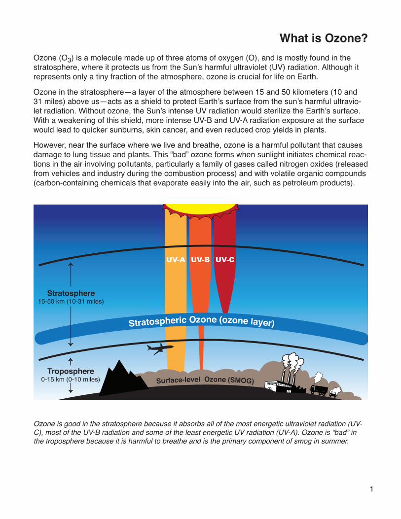
What is Ozone?Ozone (O3) is a molecule made up of three atoms of oxygen (O), and is mostly found in the stratosphere, where it protects us from the Sun’s harmful ultraviolet (UV) radiation. Although it represents only a tiny fraction of the atmosphere, ozone is crucial for life on Earth.

Ozone in the stratosphere—a layer of the atmosphere between 15 and 50 kilometers (10 and 31 miles) above us—acts as a shield to protect Earth’s surface from the sun’s harmful ultravio-let radiation. Without ozone, the Sun’s intense UV radiation would sterilize the Earth’s surface. With a weakening of this shield, more intense UV-B and UV-A radiation exposure at the surface would lead to quicker sunburns, skin cancer, and even reduced crop yields in plants.

However, near the surface where we live and breathe, ozone is a harmful pollutant that causes damage to lung tissue and plants. This “bad” ozone forms when sunlight initiates chemical reac-tions in the air involving pollutants, particularly a family of gases called nitrogen oxides (released from vehicles and industry during the combustion process) and with volatile organic compounds (carbon-containing chemicals that evaporate easily into the air, such as petroleum products).

Ozone is good in the stratosphere because it absorbs all of the most energetic ultraviolet radiation (UV-C), most of the UV-B radiation and some of the least energetic UV radiation (UV-A). Ozone is “bad” in the troposphere because it is harmful to breathe and is the primary component of smog in summer.

Surface-level Ozone (SMOG)

Stratosphere15-50 km (10-31 miles)

Troposphere0-15 km (0-10 miles)

Stratospheric Ozone (ozone layer)

UV-A UV-B UV-C

2

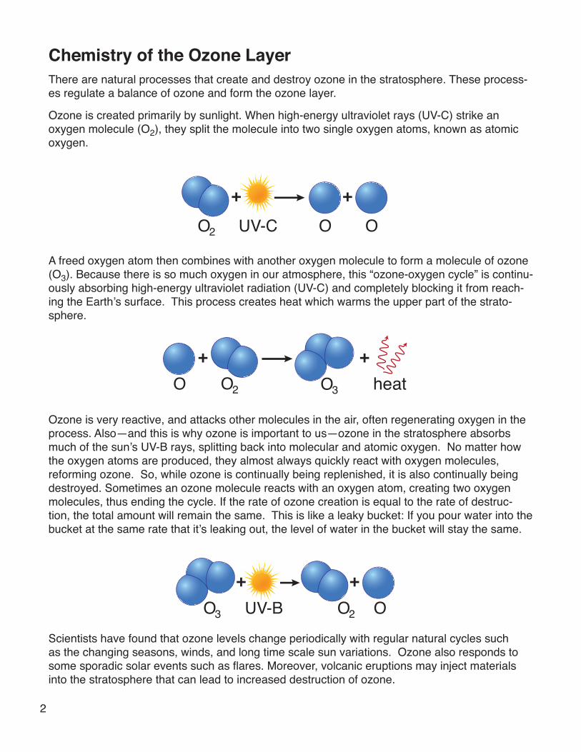
Chemistry of the Ozone Layer There are natural processes that create and destroy ozone in the stratosphere. These process-es regulate a balance of ozone and form the ozone layer.

Ozone is created primarily by sunlight. When high-energy ultraviolet rays (UV-C) strike an oxygen molecule (O2), they split the molecule into two single oxygen atoms, known as atomic oxygen.

A freed oxygen atom then combines with another oxygen molecule to form a molecule of ozone (O3). Because there is so much oxygen in our atmosphere, this “ozone-oxygen cycle” is continu-ously absorbing high-energy ultraviolet radiation (UV-C) and completely blocking it from reach-ing the Earth’s surface. This process creates heat which warms the upper part of the strato-sphere.

Ozone is very reactive, and attacks other molecules in the air, often regenerating oxygen in the process. Also—and this is why ozone is important to us—ozone in the stratosphere absorbs much of the sun’s UV-B rays, splitting back into molecular and atomic oxygen. No matter how the oxygen atoms are produced, they almost always quickly react with oxygen molecules, reforming ozone. So, while ozone is continually being replenished, it is also continually being destroyed. Sometimes an ozone molecule reacts with an oxygen atom, creating two oxygen molecules, thus ending the cycle. If the rate of ozone creation is equal to the rate of destruc-tion, the total amount will remain the same. This is like a leaky bucket: If you pour water into the bucket at the same rate that it’s leaking out, the level of water in the bucket will stay the same.

Scientists have found that ozone levels change periodically with regular natural cycles such as the changing seasons, winds, and long time scale sun variations. Ozone also responds to some sporadic solar events such as flares. Moreover, volcanic eruptions may inject materials into the stratosphere that can lead to increased destruction of ozone.

+ +

OO2 UV-C O

O2O+ +

O3 heat

O2O3

+ +

UV-B O+

V

3

Chlorofluorocarbons (CFCs)In the 1970’s, scientists suspected that reactions involving man-made chlorine-containing com-pounds could upset this balance leading to lower levels of ozone in the stratosphere. Think again of the “leaky bucket.” Putting additional ozone-destroying compounds into the atmosphere is like increasing the size of the holes in our “bucket” of ozone. The larger holes cause ozone to leak out at a faster rate than ozone is being created. Consequently, the level of ozone protecting us from ultraviolet radiation decreases. The ozone destroyed by manmade emissions is compa-rable or more than the amount destroyed by natural processes.

Human production of chlorine-containing chemicals, such as chlorofluorocarbons (CFCs), has added an additional factor that destroys ozone. CFCs are molecules made up of chlorine, fluo-rine and carbon. Because they are extremely stable molecules, CFCs do not react with other chemicals in the lower atmosphere, but exposure to ultraviolet radiation in the stratosphere breaks them apart, releasing chlorine atoms.

Free chlorine (Cl) atoms then react with ozone molecules, taking one oxygen atom to form chlo-rine monoxide (ClO) and leaving an oxygen molecule (O2).

If each chlorine atom released from a CFC molecule destroyed only one ozone molecule, CFCs would pose very little threat to the ozone layer. However, when a chlorine monoxide molecule encounters a free atom of oxygen, the oxygen atom breaks up the chlorine monoxide, stealing the oxygen atom and releasing the chlorine atom back into the stratosphere to destroy another ozone molecule. These two reactions happen over and over again, so that a single atom of chlorine, acting as a catalyst, destroys many molecules (about 100,000) of ozone.

Fortunately, chlorine atoms do not remain in the stratosphere forever. Free chlorine atoms react with gases, such as methane (CH4), and get bound up into hydrogen chloride (HCl) molecules. These molecules eventually end up back in the troposphere where they are washed away by rain. Therefore, if humans stop putting CFCs and other ozone-destroying chemicals into the stratosphere, stratospheric ozone will eventually return to its earlier, higher values.

O2O3

+ +

ClOCl

O2O+ +

ClO Cl

4

Measuring Ozone in the Earth’s AtmosphereScientists have been measuring ozone since the 1920’s using ground-based instruments that look skyward. Data from these instruments, although useful in learning about ozone, only tell us about the ozone above their sites, and do not provide a picture of global ozone concentrations. To get a global view of ozone concentrations and its distribution, scientists use data from satellites.

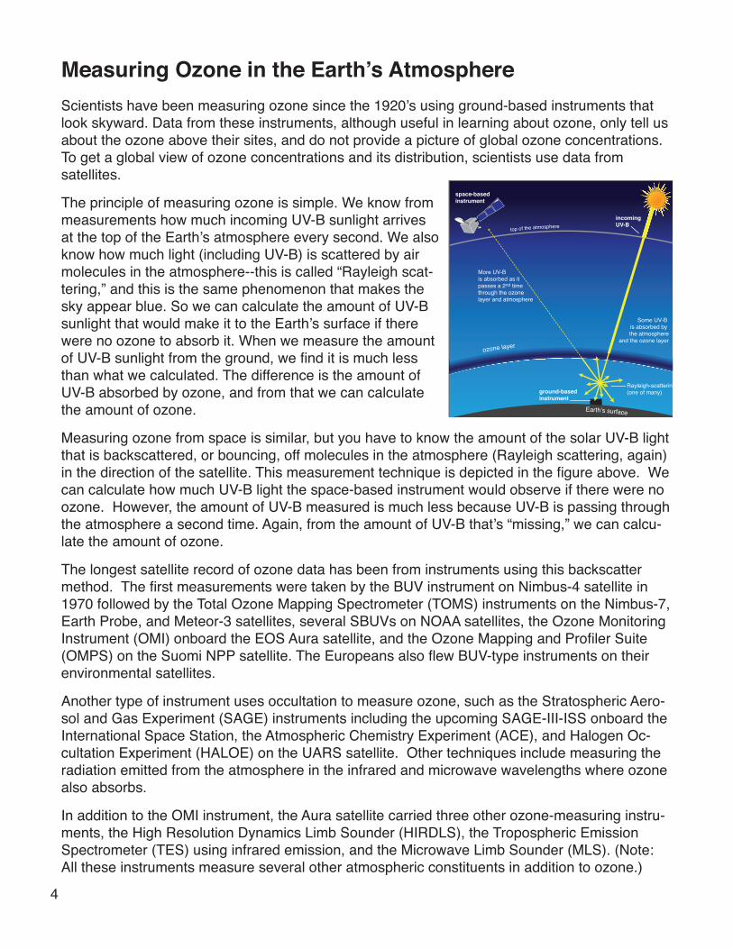
The principle of measuring ozone is simple. We know from measurements how much incoming UV-B sunlight arrives at the top of the Earth’s atmosphere every second. We also know how much light (including UV-B) is scattered by air molecules in the atmosphere--this is called “Rayleigh scat-tering,” and this is the same phenomenon that makes the sky appear blue. So we can calculate the amount of UV-B sunlight that would make it to the Earth’s surface if there were no ozone to absorb it. When we measure the amount of UV-B sunlight from the ground, we find it is much less than what we calculated. The difference is the amount of UV-B absorbed by ozone, and from that we can calculate the amount of ozone.

Measuring ozone from space is similar, but you have to know the amount of the solar UV-B light that is backscattered, or bouncing, off molecules in the atmosphere (Rayleigh scattering, again) in the direction of the satellite. This measurement technique is depicted in the figure above. We can calculate how much UV-B light the space-based instrument would observe if there were no ozone. However, the amount of UV-B measured is much less because UV-B is passing through the atmosphere a second time. Again, from the amount of UV-B that’s “missing,” we can calcu-late the amount of ozone.

The longest satellite record of ozone data has been from instruments using this backscatter method. The first measurements were taken by the BUV instrument on Nimbus-4 satellite in 1970 followed by the Total Ozone Mapping Spectrometer (TOMS) instruments on the Nimbus-7, Earth Probe, and Meteor-3 satellites, several SBUVs on NOAA satellites, the Ozone Monitoring Instrument (OMI) onboard the EOS Aura satellite, and the Ozone Mapping and Profiler Suite (OMPS) on the Suomi NPP satellite. The Europeans also flew BUV-type instruments on their environmental satellites.

Another type of instrument uses occultation to measure ozone, such as the Stratospheric Aero-sol and Gas Experiment (SAGE) instruments including the upcoming SAGE-III-ISS onboard the International Space Station, the Atmospheric Chemistry Experiment (ACE), and Halogen Oc-cultation Experiment (HALOE) on the UARS satellite. Other techniques include measuring the radiation emitted from the atmosphere in the infrared and microwave wavelengths where ozone also absorbs.

In addition to the OMI instrument, the Aura satellite carried three other ozone-measuring instru-ments, the High Resolution Dynamics Limb Sounder (HIRDLS), the Tropospheric Emission Spectrometer (TES) using infrared emission, and the Microwave Limb Sounder (MLS). (Note: All these instruments measure several other atmospheric constituents in addition to ozone.)

ground-basedinstrument

Rayleigh-scattering(one of many)

More UV-Bis absorbed as it passes a 2nd timethrough the ozonelayer and atmosphere

space-basedinstrument

ozone layer

Earth’s surface

top of the atmosphere

Some UV-B is absorbed by the atmosphere

and the ozone layer

incoming UV-B

5

How the Ozone Hole formsThe Ozone Hole is not really a “hole” but a thinning of the ozone layer over the south polar region. Every year, since at least 1978, there is a sudden, rapid decrease in the stratospheric ozone levels at the end of the Antarctic winter.

During the long winter months of darkness over the Antarctic, atmospheric temperatures drop, creating unique conditions for chemical reactions that are not found anywhere else in the atmo-sphere. The wind in the stratosphere over the polar region intensifies and forms a polar vortex, which circulates around the pole. The transition from inside to outside the polar vortex creates a wind barrier that isolates the air inside the vortex and also results in very cold temperatures.

At temperatures below -78°C, thin clouds made of mixtures of ice, nitric acid, and sulfuric acid form in the stratosphere. Chemical reactions on the surfaces of these ice crystals convert chlorine-containing compounds like HCl, which is harmless to ozone, into more reactive forms. When the sun rises over the Antarctic in the Spring (September), light rapidly releases free chlorine atoms into the stratosphere. A new ozone destroying cycle begins. The chlorine atoms react with ozone, creating ClO. The ClO molecules combine with each other, forming a com-pound called a dimer. Sunlight releases chlorine atoms from the dimer, and the cycle begins again. The polar vortex keeps the ozone-depleted air inside from mixing with the undepleted air outside the vortex.

The ozone destruction continues within the polar vortex until the ozone levels approaches zero at the altitudes where reactions on the thin clouds have released chlorine atoms. Once ozone has reached such a low level, the chlorine atoms react with methane, filling the vortex with HCl. The low ozone persists until the vortex weakens and breaks apart. Then the ozone levels in the polar stratosphere begin to return to pre-September levels due to the increase in solar UV and the mixing of polar and nonpolar air.

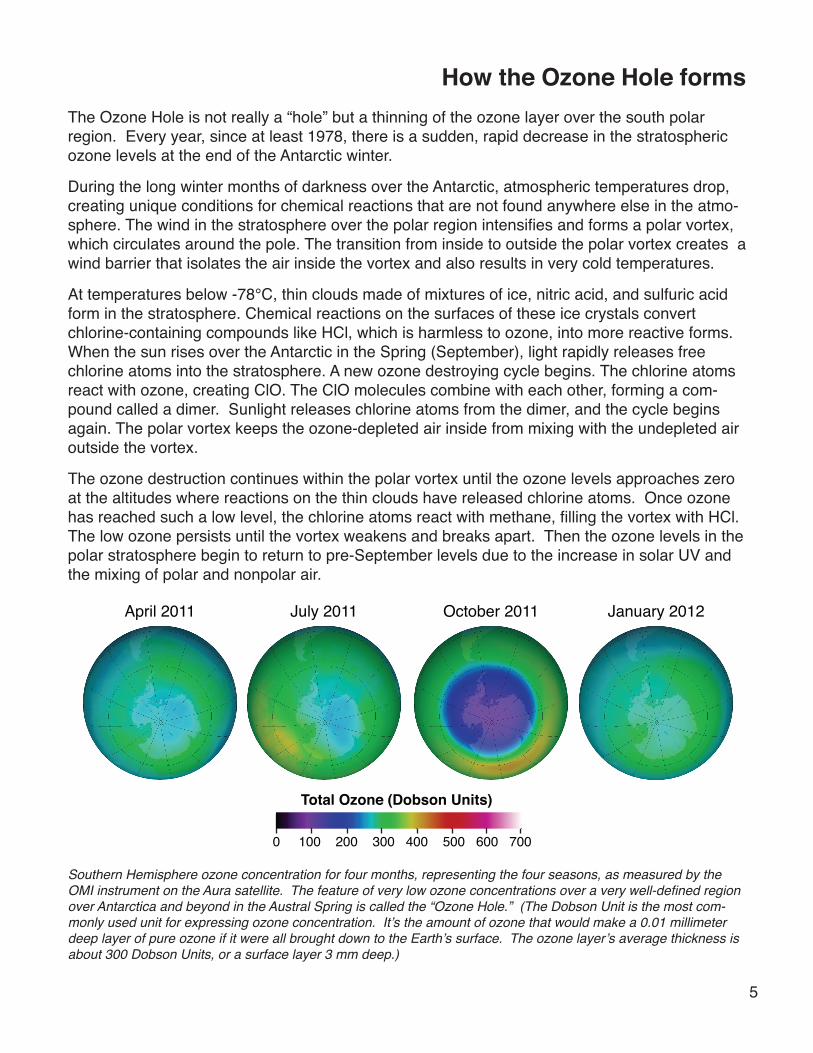
Southern Hemisphere ozone concentration for four months, representing the four seasons, as measured by the OMI instrument on the Aura satellite. The feature of very low ozone concentrations over a very well-defined region over Antarctica and beyond in the Austral Spring is called the “Ozone Hole.” (The Dobson Unit is the most com-monly used unit for expressing ozone concentration. It’s the amount of ozone that would make a 0.01 millimeter deep layer of pure ozone if it were all brought down to the Earth’s surface. The ozone layer’s average thickness is about 300 Dobson Units, or a surface layer 3 mm deep.)

April 2011 July 2011 October 2011 January 2012

0 100 200 300 400 500 600 700

Total Ozone (Dobson Units)

6

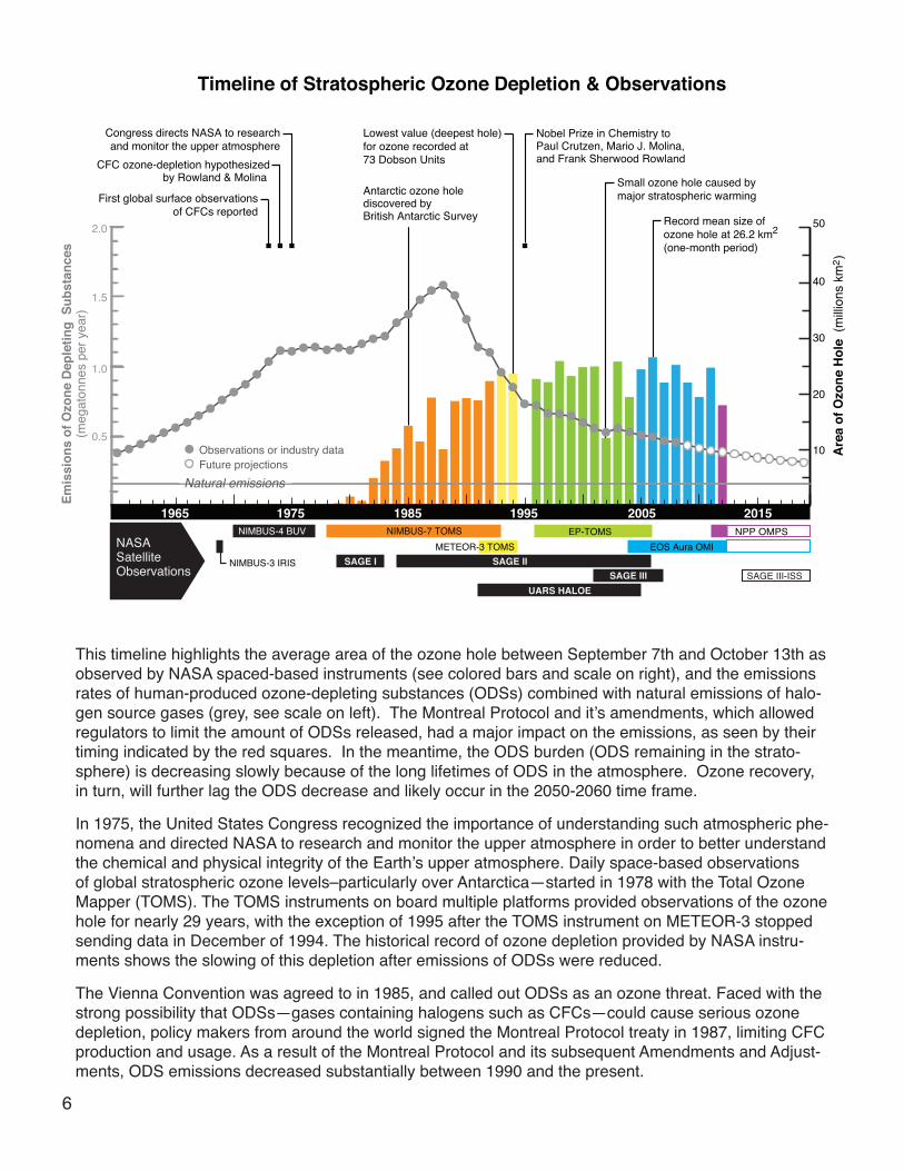
Nobel Prize in Chemistry toPaul Crutzen, Mario J. Molina, and Frank Sherwood Rowland

Antarctic ozone hole discovered byBritish Antarctic Survey

CFC ozone-depletion hypothesizedby Rowland & Molina

First global surface observationsof CFCs reported

Congress directs NASA to research and monitor the upper atmosphere

Small ozone hole caused by major stratospheric warming

Record mean size of ozone hole at 26.2 km2 (one-month period)

Lowest value (deepest hole) for ozone recorded at 73 Dobson Units

NIMBUS-3 IRIS

EP-TOMSNIMBUS-7 TOMSMETEOR-3 TOMS EOS Aura OMI

NPP OMPSNASASatelliteObservations

SAGE I SAGE IISAGE III SAGE III-ISS

UARS HALOE

NIMBUS-4 BUV1965 1975 1985 1995 2005 2015

Emis

sion

s of

Ozo

ne D

eple

ting

Sub

stan

ces

(meg

aton

nes

per y

ear)

Are

a of

Ozo

ne H

ole

(milli

ons

km2 )

Timeline of Stratospheric Ozone Depletion & Observations

2.0

0.510

20

30

40

50

1.0

1.5

Observations or industry dataFuture projections

Natural emissions

This timeline highlights the average area of the ozone hole between September 7th and October 13th as observed by NASA spaced-based instruments (see colored bars and scale on right), and the emissions rates of human-produced ozone-depleting substances (ODSs) combined with natural emissions of halo-gen source gases (grey, see scale on left). The Montreal Protocol and it’s amendments, which allowed regulators to limit the amount of ODSs released, had a major impact on the emissions, as seen by their timing indicated by the red squares. In the meantime, the ODS burden (ODS remaining in the strato-sphere) is decreasing slowly because of the long lifetimes of ODS in the atmosphere. Ozone recovery, in turn, will further lag the ODS decrease and likely occur in the 2050-2060 time frame.

In 1975, the United States Congress recognized the importance of understanding such atmospheric phe-nomena and directed NASA to research and monitor the upper atmosphere in order to better understand the chemical and physical integrity of the Earth’s upper atmosphere. Daily space-based observations of global stratospheric ozone levels–particularly over Antarctica—started in 1978 with the Total Ozone Mapper (TOMS). The TOMS instruments on board multiple platforms provided observations of the ozone hole for nearly 29 years, with the exception of 1995 after the TOMS instrument on METEOR-3 stopped sending data in December of 1994. The historical record of ozone depletion provided by NASA instru-ments shows the slowing of this depletion after emissions of ODSs were reduced.

The Vienna Convention was agreed to in 1985, and called out ODSs as an ozone threat. Faced with the strong possibility that ODSs—gases containing halogens such as CFCs—could cause serious ozone depletion, policy makers from around the world signed the Montreal Protocol treaty in 1987, limiting CFC production and usage. As a result of the Montreal Protocol and its subsequent Amendments and Adjust-ments, ODS emissions decreased substantially between 1990 and the present.

7

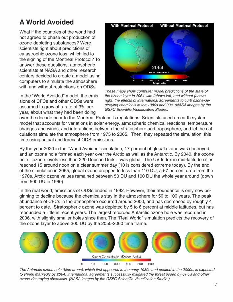
A World AvoidedWhat if the countries of the world had not agreed to phase out production of ozone-depleting substances? Were scientists right about predictions of catastrophic ozone loss, which led to the signing of the Montreal Protocol? To answer these questions, atmospheric scientists at NASA and other research centers decided to create a model using computers to simulate the atmosphere with and without restrictions on ODSs.

In the “World Avoided” model, the emis-sions of CFCs and other ODSs were assumed to grow at a rate of 3% per year, about what they had been doing over the decade prior to the Montreal Protocol’s regulations. Scientists used an earth system model that accounts for variations in solar energy, atmospheric chemical reactions, temperature changes and winds, and interactions between the stratosphere and troposphere, and let the cal-culations simulate the atmosphere from 1975 to 2065. Then, they repeated the simulation, this time using actual and forecast ODS emissions.

By the year 2020 in the “World Avoided” simulation, 17 percent of global ozone was destroyed, and an ozone hole formed each year over the Arctic as well as the Antarctic. By 2040, the ozone hole—ozone levels less than 220 Dobson Units—was global. The UV Index in mid-latitude cities reached 15 around noon on a clear summer day (10 is considered extreme today). By the end of the simulation in 2065, global ozone dropped to less than 110 DU, a 67 percent drop from the 1970s. Arctic ozone values remained between 50 DU and 100 DU the whole year around (down from 500 DU in 1960).

In the real world, emissions of ODSs ended in 1992. However, their abundance is only now be-ginning to decline because the chemicals stay in the atmosphere for 50 to 100 years. The peak abundance of CFCs in the atmosphere occurred around 2000, and has decreased by roughly 4 percent to date. Stratospheric ozone was depleted by 5 to 6 percent at middle latitudes, but has rebounded a little in recent years. The largest recorded Antarctic ozone hole was recorded in 2006, with slightly smaller holes since then. The “Real World” simulation predicts the recovery of the ozone layer to above 300 DU by the 2050-2060 time frame.

With Montreal Protocol Without Montreal Protocol

These maps show computer model predictions of the state of the ozone layer in 2064 with (above left) and without (above right) the effects of international agreements to curb ozone-de-stroying chemicals in the 1980s and 90s. (NASA images by the GSFC Scientific Visualization Studio.)

0 100 200 300 400 500 600

Ozone Concentration (Dobson Units)

The Antarctic ozone hole (blue areas), which first appeared in the early 1980s and peaked in the 2000s, is expected to shrink markedly by 2064. International agreements successfully mitigated the threat posed by CFCs and other ozone-destroying chemicals. (NASA images by the GSFC Scientific Visualization Studio.)

Exploring Color MapsUsing Stratospheric Ozone Data

National Aeronautics and Space Administration

Objectives After completing this activity, students should be able to

• describe why color maps are used to visualize data • interpret data using a color mapped image• compare and evaluate different color scales

Standards (Grades 9-12)NGSS: Practice 4 Analyzing and Interpreting DataAAAS: 12E/H2 Check graphs to see that they do not

misrepresent results by using inappropriate scales. AAAS: 11C/H4 Graphs and equations are useful ways

for depicting and analyzing patterns of change. NSES: Unifying Concepts and Processes Standard:

Evidence, models, and explanation.NSES: Content Standard E: Understandings about sci-

ence and technology

Materials• Images on the Ozone Hole poster http://aura.gsfc.nasa.gov/ozoneholeposter/• Color by Number Worksheet• 7 colored pencils / crayons• Sea Surface Temperature images

Engage Ask questions about the front of the poster. When was the ozone hole the smallest? (1979) When did the ozone hole grow the fastest? (1981–1985, pattern of growth, no shrinking) What year had the largest ozone hole? (2006) Ask students to provide evidence for their answers. (the graph, the globes, the colors) Ask how these helped an-swer the questions.

Explore Using the “Color by Number” worksheet, ask students to create a visual representation that accurately communi-cates the size of the ozone hole. Invite students to make up their own color scale. The seven ranges of ozone data

This lesson will introduce students to the use of color maps to visualize data about stratospheric ozone. Scientists use colors and other representations for data to help interpret and visualize information. Data are mapped to colors and other representations to help the mind interpret this information. Sometimes this means creating an image that looks much like an aerial photo of the planet’s surface, but other data are best mapped to a color scale. Students will create their own color map and discover that selecting a good color scale is both essential to understanding data and to accurately communicating science.

For more information, visit:http://aura.gsfc.nasa.gov/ozoneholeposter/http://ozonewatch.gsfc.nasa.govhttp://earthobservatory.nasa.gov

may be divided any way they like. Ranges don’t have to start at zero and don’t have to be even units. They can choose any colors or shades of colors they like. (If the activity is being done by an individual student, color two maps with different scales.) Encourage students to think about the range and why they choose it.

Post the back of the poster so students can gather more information about the ozone hole to help them design their color scales. You can also post some ozone facts on the board.

Ozone facts: The average ozone levels over the en-tire globe is 300 Dobson Units. Values lower than 220 Dobson Units are considered part of the ozone hole. In 2006, the worst year for ozone depletion to date, the lowest values of 84 Dobson Units were observed.

Explain Post student drawings on the wall and compare. Do any look like there is almost no hole? Which one is easiest to understand? Why? Hardest to understand? Why? Why not use the same color for all types of data? Explain how the different color scales help us to visualize data by drawing attention to what is important, such as the loca-tion of the ozone hole. However, color can also be de-ceptive, such as when there is a break in a color scale that stands out where there is nothing really unique about the data.

Evaluate Looking back at the poster, ask students “Why was this particular color scale chosen?” (There is a noticeable break from light to dark blue at 220 DU, where values

lower than 220 DU are considered to be the “ozone hole.”) Ask students to think about their scales and de-scribe why they choose certain colors and data ranges. Which data were emphasized or de-emphasized in their color maps?

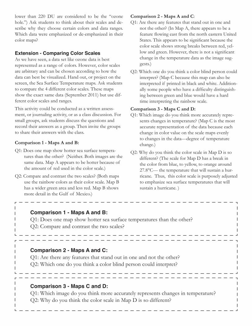
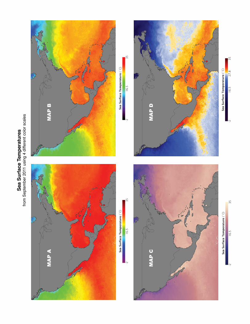
Extension - Comparing Color ScalesAs we have seen, a data set like ozone data is best represented as a range of colors. However, color scales are arbitrary and can be chosen according to how the data can best be visualized. Hand out, or project on the screen, the Sea Surface Temperature maps. Ask students to compare the 4 different color scales. These maps show the exact same data (September 2011) but use dif-ferent color scales and ranges.

This activity could be conducted as a written assess-ment, or journaling activity, or as a class discussion. For small groups, ask students discuss the questions and record their answers as a group. Then invite the groups to share their answers with the class.

Comparison 1 - Maps A and B:

Q1: Does one map show hotter sea surface tempera-tures than the other? (Neither. Both images are the same data. Map A appears to be hotter because of the amount of red used in the color scale.)

Q2: Compare and contrast the two scales? (Both maps use the rainbow colors as their color scale. Map B has a wider green area and less red. Map B shows more detail in the Gulf of Mexico.)

Comparison 2 - Maps A and C:Q1: Are there any features that stand out in one and

not the other? (In Map A, there appears to be a feature flowing east from the north eastern United States. This appears to be significant because the color scale shows strong breaks between red, yel-low and green. However, there is not a significant change in the temperature data as the image sug-gests.)

Q2: Which one do you think a color blind person could interpret? (Map C because this map can also be interpreted if printed in black and white. Addition-ally some people who have a difficulty distinguish-ing between green and blue would have a hard time interpreting the rainbow scale.

Comparison 3 - Maps C and D:Q1: Which image do you think more accurately repre-

sents changes in temperature? (Map C is the most accurate representation of the data because each change in color value on the scale maps evenly to changes in the data —degree of temperature change.)

Q2: Why do you think the color scale in Map D is so different? (The scale for Map D has a break in the color from blue, to yellow, to orange around 27.8°C— the temperature that will sustain a hur-ricane. Thus, this color scale is purposely adjusted to emphasize sea surface temperatures that will sustain a hurricane. )

Comparison 1 - Maps A and B:Q1: Does one map show hotter sea surface temperatures than the other? Q2: Compare and contrast the two scales?

Comparison 2 - Maps A and C:Q1: Are there any features that stand out in one and not the other? Q2: Which one do you think a color blind person could interpret?

Comparison 3 - Maps C and D:Q1: Which image do you think more accurately represents changes in temperature? Q2: Why do you think the color scale in Map D is so different?

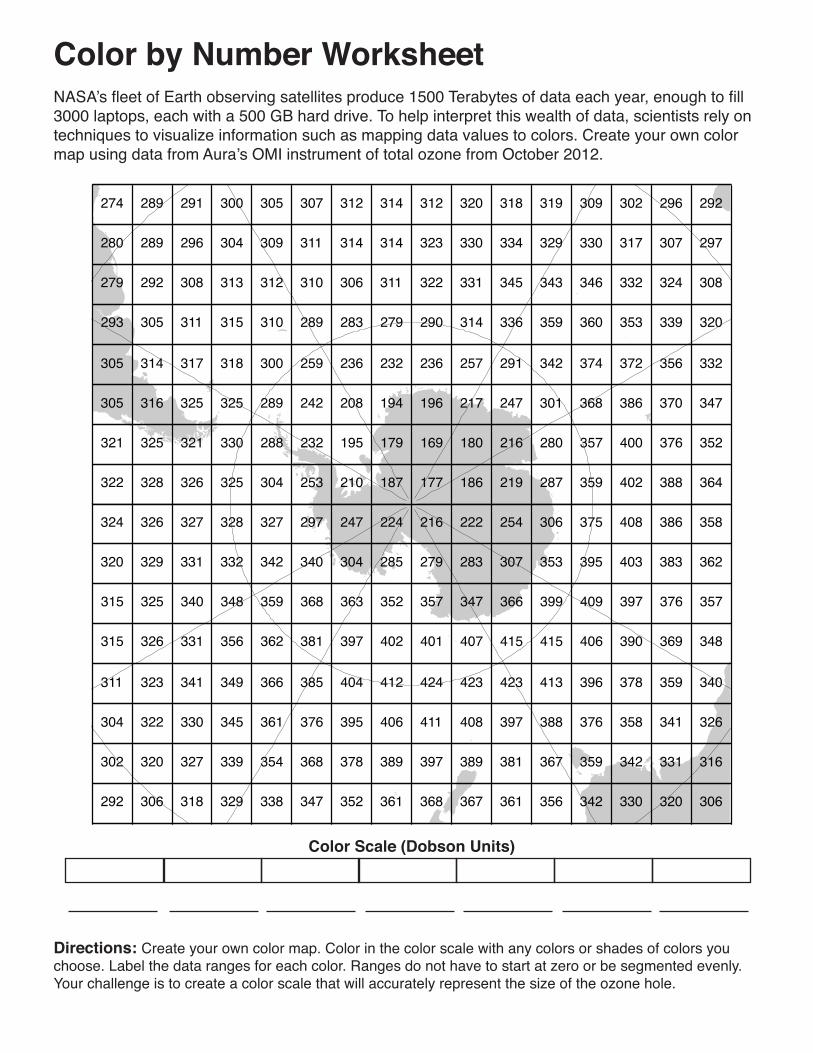
Directions: Create your own color map. Color in the color scale with any colors or shades of colors you choose. Label the data ranges for each color. Ranges do not have to start at zero or be segmented evenly. Your challenge is to create a color scale that will accurately represent the size of the ozone hole.

Color Scale (Dobson Units)

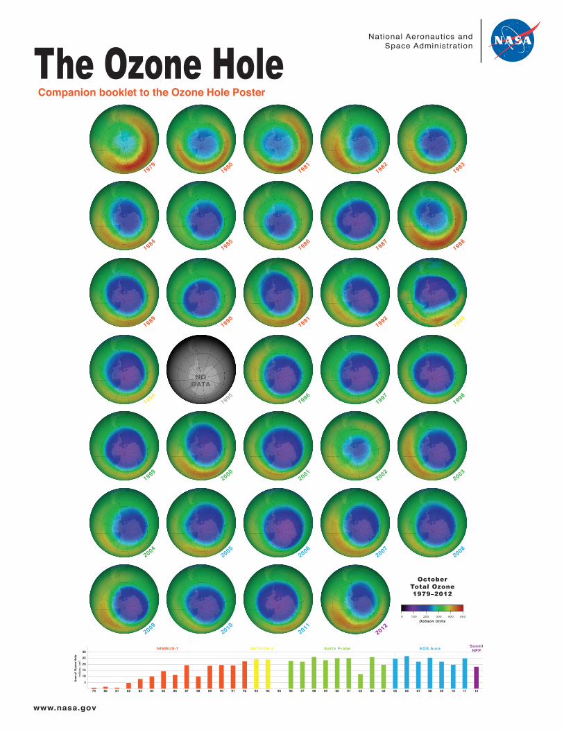
Color by Number WorksheetNASA’s fleet of Earth observing satellites produce 1500 Terabytes of data each year, enough to fill 3000 laptops, each with a 500 GB hard drive. To help interpret this wealth of data, scientists rely on techniques to visualize information such as mapping data values to colors. Create your own color map using data from Aura’s OMI instrument of total ozone from October 2012.

292 306 318 329 338 347 352 361 368 367 361 356 342 330 320 306

302 320 327 339 354 368 378 389 397 389 381 367 359 342 331 316

304 322 330 345 361 376 395 406 411 408 397 388 376 358 341 326

311 323 341 349 366 385 404 412 424 423 423 413 396 378 359 340

315 326 331 356 362 381 397 402 401 407 415 415 406 390 369 348

315 325 340 348 359 368 363 352 357 347 366 399 409 397 376 357

320 329 331 332 342 340 304 285 279 283 307 353 395 403 383 362

324 326 327 328 327 297 247 224 216 222 254 306 375 408 386 358

322 328 326 325 304 253 210 187 177 186 219 287 359 402 388 364

321 325 321 330 288 232 195 179 169 180 216 280 357 400 376 352

305 316 325 325 289 242 208 194 196 217 247 301 368 386 370 347

305 314 317 318 300 259 236 232 236 257 291 342 374 372 356 332

293 305 311 315 310 289 283 279 290 314 336 359 360 353 339 320

279 292 308 313 312 310 306 311 322 331 345 343 346 332 324 308

280 289 296 304 309 311 314 314 323 330 334 329 330 317 307 297

292274 289 291 300 305 307 312 314 312 320 318 319 309 302 296

Sea

Surf

ace

Tem

pera

ture

sfro

m S

epte

mbe

r 201

1 us

ing

4 di

ffere

nt c

olor

sca

les

MA

P A

MA

P B

MA

P C

MA

P D

About the Poster:

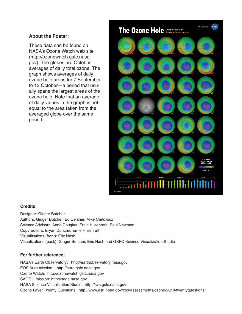
These data can be found on NASA’s Ozone Watch web site (http://ozonewatch.gsfc.nasa.gov). The globes are October averages of daily total ozone. The graph shows averages of daily ozone hole areas for 7 September to 13 October—a period that usu-ally spans the largest areas of the ozone hole. Note that an average of daily values in the graph is not equal to the area taken from the averaged globe over the same period.

For further reference:NASA’s Earth Observatory: http://earthobservatory.nasa.govEOS Aura mission: http://aura.gsfc.nasa.govOzone Watch: http://ozonewatch.gsfc.nasa.govSAGE II mission: http://sage.nasa.govNASA Science Visualization Studio: http://svs.gsfc.nasa.govOzone Layer Twenty Questions: http://www.esrl.noaa.gov/csd/assessments/ozone/2010/twentyquestions/

Credits:Designer: Ginger ButcherAuthors: Ginger Butcher, Ed Celarier, Mike Carlowicz Science Advisors: Anne Douglas, Ernie Hilsenrath, Paul NewmanCopy Editors: Bryan Duncan, Ernie HilsenrathVisualizations (front): Eric NashVisualizations (back): Ginger Butcher, Eric Nash and GSFC Science Visualization Studio